Harmonized retrieval of middle atmospheric ozone from two microwave radiometers in Switzerland

We present new harmonized ozone time series from two ground-based microwave radiometers in Switzerland: GROMOS and SOMORA. Both instruments have measured hourly ozone profiles in the middle atmosphere (20–75 km) for more than 2 decades. As inconsistencies in long-term trends derived from these two instruments were detected, a harmonization project was initiated in 2019. The goal was to fully harmonize the data processing of GROMOS and SOMORA to better understand and possibly reduce the discrepancies between the two data records. The harmonization has been completed for the data from 2009 until 2022 and has been successful at reducing the differences observed between the two time series. It also explains the remaining differences between the two instruments and flags their respective anomalous measurement periods in order to adapt their consideration for future trend computations.

We describe the harmonization and the resulting time series in detail. We also highlight the improvements in the ozone retrievals with respect to the previous data processing. In the stratosphere and lower mesosphere, the seasonal ozone relative differences between the two instruments are now within 10 % and show good correlation (R > 0.7) (except during summertime). We also perform a comparison of these new data series against measurements from the Microwave Limb Sounder (MLS) and Solar Backscatter Ultraviolet Radiometer (SBUV) satellite instruments over Switzerland. Seasonal mean differences with MLS and SBUV are within 10 % in the stratosphere and lower mesosphere up to 60 km and increase rapidly above that point.

1 Introduction

Ozone is a trace gas of great importance in the earth's atmosphere. It shields the surface of our planet from most of the sun's harmful ultraviolet radiation by absorbing it in the stratosphere (the “ozone layer”) and consequently allowing life out of water. In the second half of the 20th century, it was suggested that anthropogenic emissions of certain chemical compounds, the commonly called ozone-depleting substances (ODSs), were threatening this protective layer (Molina and Rowland, 1974; Crutzen, 1970; Farman et al., 1985; Solomon et al., 1986). As a result, severe depletion of the ozone layer was observed in the springtime over the Antarctic and led to the banning of ODS emissions formalized in the Montreal Protocol in 1987.

Since then, there has been an increased interest in the monitoring of ozone in the middle atmosphere to assess the effect of the Montreal Protocol. The reduction of ODS emissions has led to a decrease in total chlorine concentration since 1997, whereas the increasing greenhouse gases concentration is cooling the upper stratosphere (Anderson et al., 2000; Solomon et al., 2006). From the existing knowledge in middle-atmospheric chemistry, the combination of both factors should lead to an observable recovery or even super recovery of ozone concentration at these altitudes (Eyring et al., 2010). In fact, over the polar regions, the stratospheric ozone concentrations have already begun their recovery towards pre-industrial levels (Solomon et al., 2016). Over the mid-latitudes, the situation is less obvious, and ozone recovery seems to differ depending on the altitude and the geographical area of interest (Braesicke et al., 2018; Petropavlovskikh et al., 2019; Tummon et al., 2015). In the upper stratosphere, the latest observations agree on a positive trend of ozone concentration despite a high variability in its significance and magnitude (Fahey et al., 2018; Steinbrecht et al., 2017; Bernet et al., 2019; Godin-Beekmann et al., 2022). In contrast, no clear indication of ozone recovery has been reported yet in the lower stratosphere and some observational evidence of further decline in this region were even reported (Ball et al., 2018). In the context of climate change, there also remain many unknowns regarding the influence of long-term dynamic and composition changes on middle-atmospheric ozone trends depending on the region (von der Gathen et al., 2021). In regards to these uncertainties, there is still a high need for accurate and long-term time series in the research field.

Microwave ground-based radiometers (MWRs) provide continuous, all-weather measurements of ozone in the middle atmosphere and are therefore well suited to estimate long-term trends and cross-validate satellite measurements (Hocke et al., 2007). Compared to other ground-based measurement techniques, they are able to retrieve ozone profiles from the stratosphere well into the mesosphere with a high temporal resolution but at the cost of a quite low vertical resolution.

In Switzerland, two ozone MWRs have operated for more than 20 years in the vicinity of each other (ca. 40 km): the GROund-based Millimeter-wave Ozone Spectrometer (GROMOS) in Bern and the Stratospheric Ozone MOnitoring RAdiometer (SOMORA) in Payerne (Fig. 1). They operate in the frame of the Network for the Detection of Atmospheric Composition Change (NDACC) (De Mazière et al., 2018). Such long-term time series of two ozone MWRs combined in such geographic proximity is unique worldwide and therefore offers the opportunity for extensive cross-validations. It also allows for more thorough investigation of measurement uncertainties, possible instrumental failures, and calibration and retrieval errors.

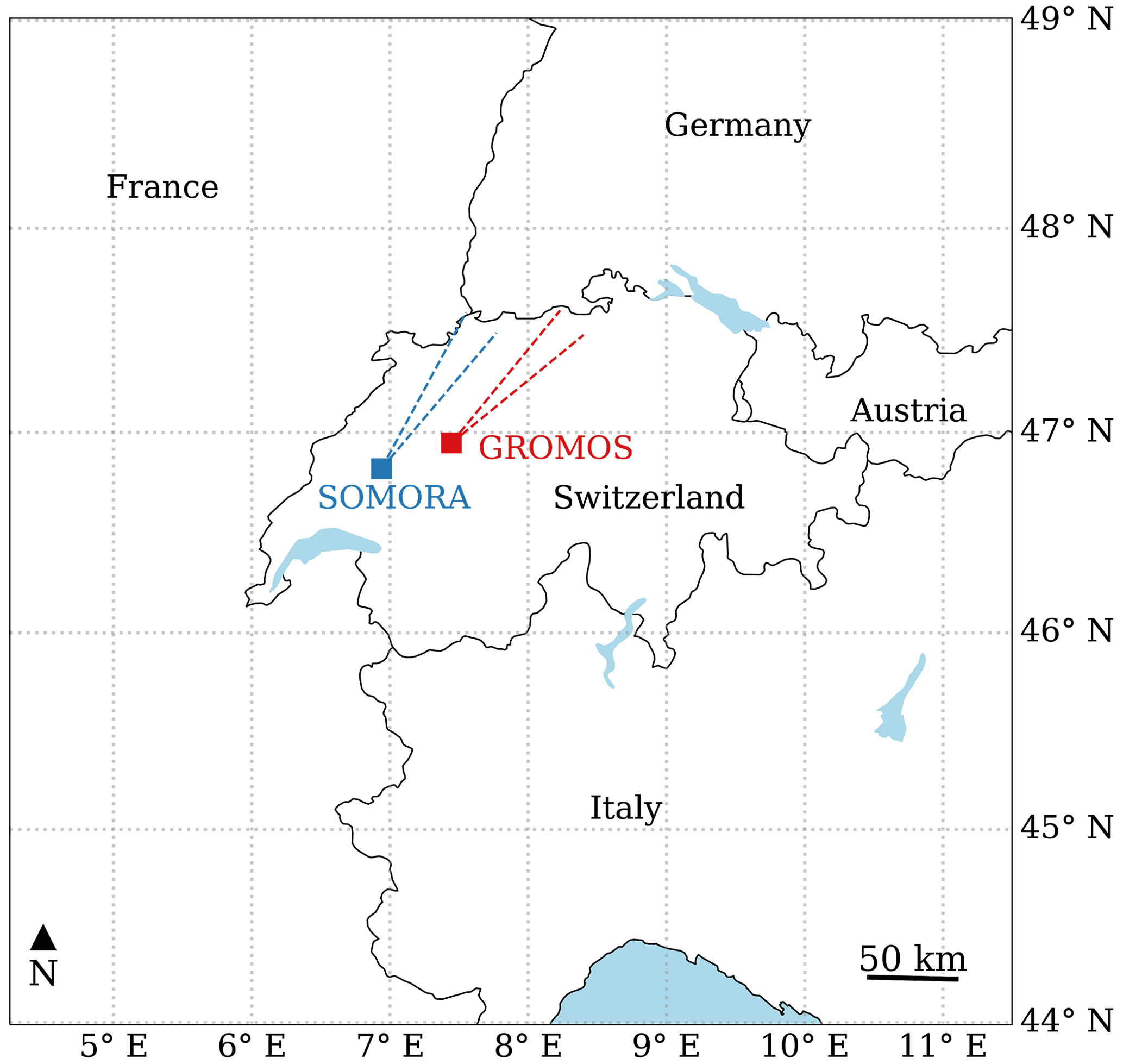
Figure 1 Location of GROMOS and SOMORA, with their approximate viewing directions.

During the first phase of the activity “Long-term Ozone Trends and Uncertainties in the Stratosphere” (LOTUS), inconsistencies were found in ozone trend estimates from these two radiometers (Petropavlovskikh et al., 2019). In addition, Bernet et al. (2019) identified some anomalous periods in the Bern time series and highlighted the need to account for these anomalies to compute more accurate trends. However, Bernet et al. (2019) did not investigate the reasons for such anomalies, and the differences between these two time series remained unexplained. Due to their geographic proximity and similar observation geometry, the differences are too big to be geophysical. The data processing, however, was quite different between the instruments, and therefore it was decided to reprocess both time series with new and harmonized algorithms. A harmonization project was initiated jointly by the operators of these two instruments in 2019 with the goal to better understand their differences.

We present and validate here the new harmonized time series for GROMOS and SOMORA focusing on the time period from the month of September 2009 until December 2021. We present the harmonization process applied to the data processing of the two radiometers, including a short description of the new calibration and retrieval routines. We also show the improvements resulting from this harmonization by comparing the new series with their previous versions. As a validation, we performed a cross-comparison between the two instruments and compared them against satellite dataset, namely from the Microwave Limb Sounder (MLS) and the Solar Backscatter Ultraviolet Radiometer (SBUV).

A detailed description of the calibration and retrievals routines has been published in the form of two research reports available on the publication database of the University of Bern (Sauvageat, 2021, 2022a), and a full documentation of the time series is available together with the data.

This paper is organized as follows. Section 2 presents the instruments, highlighting their similarities and differences. Section 3 presents the harmonization procedure applied to the calibration and retrieval routines. Section 4 presents the new harmonized ozone time series, whereas Sect. 5 presents comparisons and cross-validations against satellite measurements. Section 6 summarizes the main conclusions and gives an outlook.

2 Ozone microwave radiometry in Switzerland

Passive microwave radiometry uses the electromagnetic radiation emitted and transmitted in the microwave frequency region to derive geophysical quantities of interest. It makes this technique suitable for both surface observation of the earth from space and sounding of atmospheric trace gases, temperature or winds from satellites or ground-based instruments. Unlike other techniques, MWRs do not require UV/VIS emitting sources (e.g. sun or stars) and are able to measure during day and night. In addition, the pressure broadening effect at microwave frequencies enables the retrieval of vertical profiles of temperature, winds and abundances (e.g. Parrish et al., 1988; Connor et al., 1994; Rüfenacht et al., 2012; Krochin et al., 2022).

Ozone possesses many rotational transition lines in the microwave region. Its emission lines at 110.836 and 142.175 GHz are most often used for ground-based observations because of their line intensity and the limited effect of water vapour absorption at these frequencies.

Table 1 GROMOS and SOMORA microwave radiometers.

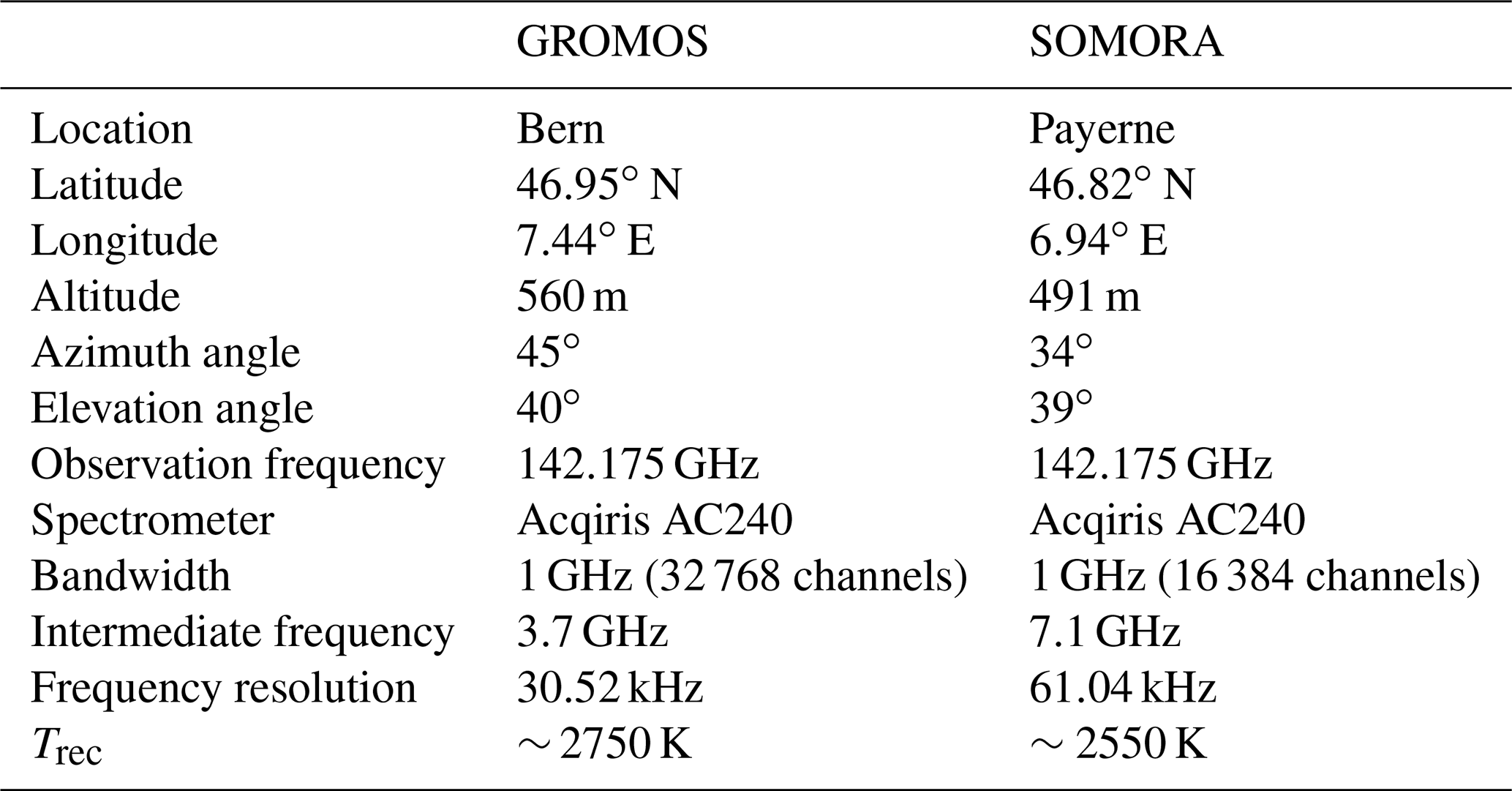
GROMOS and SOMORA have been designed and built at the Institute of Applied Physics (IAP) at the University of Bern with quite similar components (Calisesi, 2003; Peter, 1997). They observe the ozone emission line around 142 GHz to retrieve hourly ozone profiles in the stratosphere and lower mesosphere (∼ 20 to 75 km) using the optimal estimation method. GROMOS has been operated by IAP in Bern since 1994, and SOMORA has been operated by the Federal Office of Meteorology and Climatology (MeteoSwiss) in Payerne since 2000 (see locations given in Fig. 1). Both instruments are located on the Swiss Plateau, approximately 40 km from each other, where they experience similar atmospheric conditions. This can be seen by looking at the seasonal distribution of tropospheric opacities at the two sites shown in Fig. A1. The main characteristics of the two instruments are summarized in Table 1.

2.1 Spectrometers

The spectrometer is a key component of any MWR and can significantly influence its retrieval capabilities. Since 2009, both instruments use the same spectrometer, namely the Acqiris AC240 which is a digital fast Fourier transform (FFT) spectrometer (Benz et al., 2005; Muller et al., 2009). On SOMORA, it replaced an acousto-optical spectrometer in September 2009, whereas on GROMOS it replaced discrete filter banks in July 2009. In both cases, the time series were homogenized using an overlap period of roughly 2 years, and the pre-2009 time series were corrected with respect to the FFT spectrometer time series (e.g. Moreira et al., 2015; Maillard Barras et al., 2020). Whereas both instruments use the same digitizer with the same bandwidth of 1 GHz, it should be noted that the frequency resolution is 2 times higher for GROMOS than for SOMORA because GROMOS uses an in-phase quadrature (IQ) down-converter and digital sideband separation, which results in twice the number of channels (Murk et al., 2009). As a result, GROMOS could be more sensitive to ozone at higher altitudes. However, we do not see any significant difference in vertical sensitivity compared to SOMORA, possibly because of the high receiver noise, which could act as a limiting factor for extending the altitude coverage of the two instruments.

The AC240 is still being used in many MWRs; however, it is ageing and has recently been shown to produce a spectral bias compared to more recent spectrometers, most likely impacting ozone retrievals as well (Sauvageat et al., 2021). In this contribution, we only focus on the period where both instruments use the AC240, namely from September 2009 to end of 2021. Therefore, both time series should be similarly impacted by the spectrometric bias and thus should not affect the results of the comparisons between GROMOS and SOMORA. This might, however, influence the comparisons against the satellite observations, but there is unfortunately no way to confirm the amplitude of the bias on the ozone profiles at the moment.

3 Harmonization process

Discrepancies were identified between the GROMOS and SOMORA data series and trends (Bernet et al., 2019; Petropavlovskikh et al., 2019; Maillard Barras et al., 2020) for which no explanations could be found. To better understand these discrepancies, it was decided to perform a full harmonization of the data processing of GROMOS and SOMORA, from the raw data (level 0) to the ozone profiles (level 2). The idea was to harmonize the whole processing chain, including the inputs and outputs of the routine, while keeping the two data series fully independent.

The harmonization project can be separated into two distinct parts: the calibration of the radiometric data (level 0 to 1) and the retrievals of ozone profiles (level 1 to 2). Section 3.1 will briefly describe the new calibration and integration routines (see Sauvageat, 2021 for details), whereas Sect. 3.2 will describe the retrievals of ozone profiles from the calibrated spectra.

3.1 Calibration

GROMOS and SOMORA are both total power radiometers with superheterodyne receivers. They measure the atmospheric ozone emission line around 142.175 GHz and use the heterodyne principle to down convert the incoming radiation (RF signal) to an intermediate frequency (IF) by mixing with a local oscillator frequency (LO) which allows for easier signal processing.

The operation of microwave radiometers requires continuous calibration because their receivers are never perfectly stable (e.g. Ulaby and Long, 2014, chap. 7). Both instruments use a so-called hot–cold calibration scheme: using a rotating mirror fixed on a path length modulator, they are continuously switching between the atmospheric observation, a hot and a cold calibration target. In both instruments, a heated black-body kept at a constant temperature (T_hot≈310 K) is used as hot load, whereas liquid nitrogen (LN2) observation is used as cold load. Both instruments use a Martin–Pupplet interferometer (MPI) to suppress the contribution of the undesired sideband. The pathlength modulator is used to mitigate the standing waves between the receiver and the calibration targets, which are otherwise causing systematic baseline errors on the calibrated spectra. In parallel to the hot–cold calibration scheme, the instruments also perform tipping curve calibration (Ingold et al., 1998) as cross-validation for the LN2 calibration. Assuming linear transfer characteristics, the atmospheric spectral radiance can then be determined and further converted to brightness temperature using Planck's law (e.g. Ulaby and Long, 2014, chap. 6).

Despite similar designs and raw data contents, the previous calibration routines for GROMOS and SOMORA were different. Therefore, a new routine was designed to harmonize the calibration between the two instruments. The calibration essentially converts the raw spectrometer measurements to radiance intensity and integrates them together on a chosen integration time. For this new routine, the calibration results in two different data levels, namely the calibrated spectrum (level 1a) and the integrated spectrum (level 1b).

Harmonized quality control was introduced in order to identify spurious instrumental signals. It flags the most common technical problems at level 1a (e.g. noise temperature jumps, LN2 refills, LO frequency shifts) and combines them into a single instrumental flag value for level 1b (Sauvageat, 2021).

Considering instrumental issues and technical interruptions for maintenance (e.g. for LN2 refilling or instrument repairs), GROMOS and SOMORA provided good-quality hourly spectra for 87 % and 89 % of the measurements performed between 2009 and 2021, respectively. This results in more than 80 000 h of comparable retrieved ozone profiles.

3.2 Retrieval setup

In the microwave frequency range, the pressure-broadening effect of atmospheric emission lines is used to retrieve information on the atmospheric constituent profile from the calibrated microwave emission spectra. This so-called retrieval is a well-validated technique that has been successfully applied to temperature; wind; and many trace gases like O₃, CO, or H₂O (Janssen, 1993, chap. 7). Among the different retrieval techniques, we selected the optimal estimation method (OEM) following the formalism described by Rodgers (2000). This statistical method extracts the best estimate of an atmospheric profile from a set of measurements with noise, a priori information and a forward model. In addition, the OEM enables the characterization of the error budget of the retrievals (Fig. 3). In the following, we will briefly present and discuss the new harmonized retrieval setup used for GROMOS and SOMORA. More information on this setup is available in Sauvageat (2022a). For detailed information on the OEM or its application to ozone profiling instruments, the reader is redirected to Parrish et al. (1992) or Tsou et al. (1995).

3.2.1 Forward model

In the case of ground-based microwave radiometry, the forward model (FM) describes the radiative transfer physics between trace gas emissions and the instrument's receiver. We used the Atmospheric Radiative Transfer Simulator 2.4 (ARTS), an open-source software with a special focus on microwave radiative transfer simulations (Eriksson et al., 2011; Buehler et al., 2018). In addition, it offers a fully integrated OEM retrieval environment and includes many tools to help simulate and retrieve the sensor's influence on the radiometric measurements (Eriksson et al., 2006).

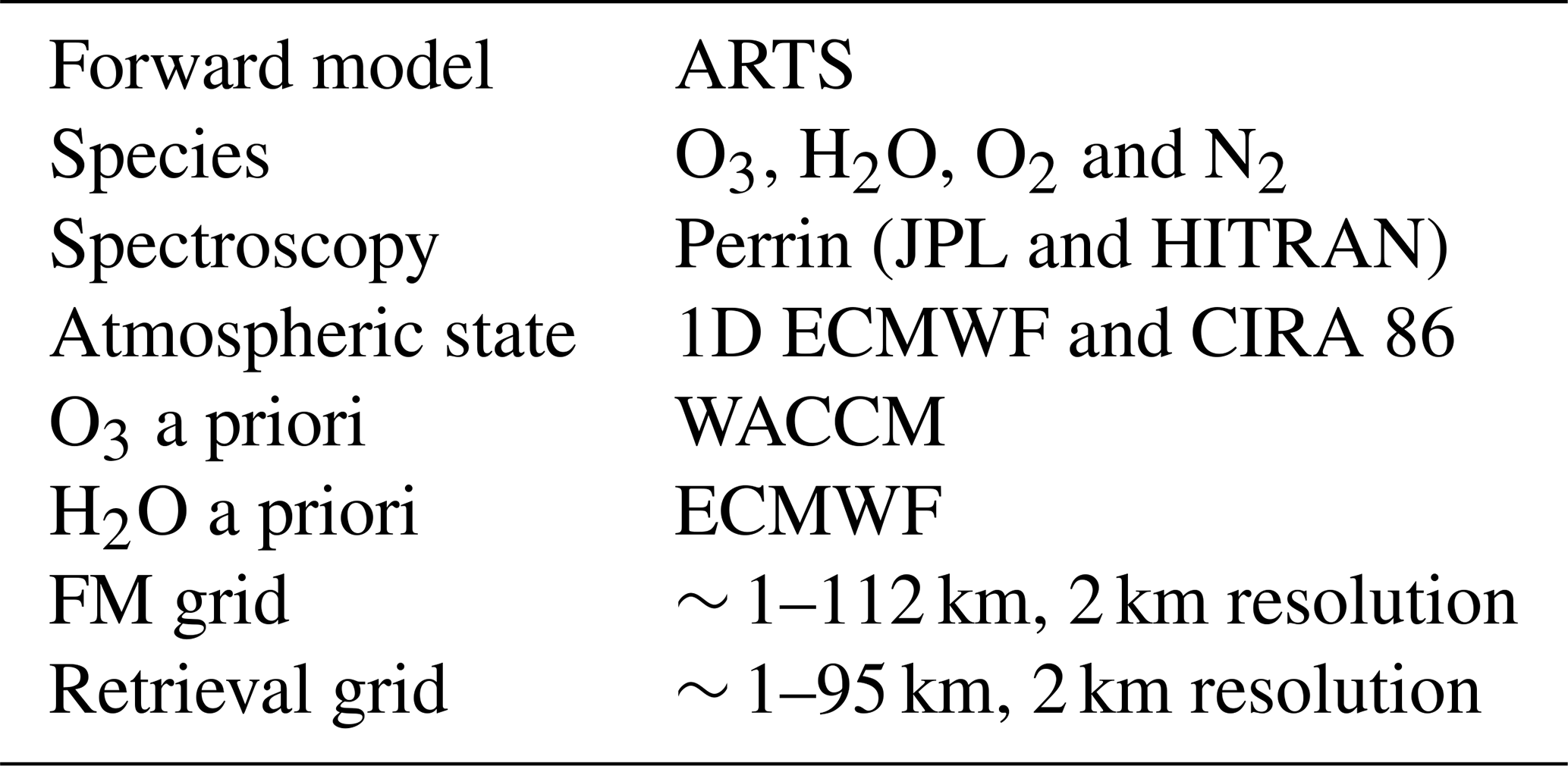
ARTS offers many possibilities to define the atmospheric state, a priori data and simulation grids. We use one-dimensional pressure and temperature profiles from the European Centre for Medium-Range Weather Forecasts (ECMWF) daily operational analysis (6 h time and 1.125^∘ spatial resolution). This dataset is limited to approximately 70 km altitude, and we therefore extend it using the COSPAR International Reference Atmosphere (CIRA-86) climatology at upper altitudes (Chandra et al., 1990). The frequency grids have been defined to cover the range of GROMOS and SOMORA spectrometers with a refined frequency resolution around the ozone line: it matches the spectrometer resolution at the line centre to optimize retrievals at higher altitudes, whereas the spectral resolution is coarser on the line wings to limit computation time.

As atmospheric species, we use ozone, water vapour, oxygen and nitrogen. For ozone, we use the spectroscopic database from Perrin et al. (2005), which is provided with ARTS 2.4 and is derived from the HITRAN and JPL spectroscopic databases. For water vapour, oxygen and nitrogen, we use the parameterizations provided within ARTS (see Buehler et al., 2005). A summary of the main retrieval parameters used for GROMOS and SOMORA can be found in Table 2, and more details are provided in Sauvageat (2022a).

Table 2 Main parameters used in GROMOS and SOMORA retrievals.

3.2.2 Ozone retrieval

The main retrieval quantity is hourly ozone volume mixing ratio (VMR) from the stratosphere to the lower mesosphere, i.e. between ∼ 100 and 0.01 hPa. The a priori are monthly ozone profiles extracted from free-running simulations of the Whole Atmosphere Community Climate Model (WACCM) as described in Schanz et al. (2014). Further, depending on the local solar time, we either use a daytime or nighttime a priori ozone profile. The a priori covariance matrix for ozone varies with atmospheric pressure in order to optimize the information from the measurements in the stratosphere and lower mesosphere. It includes exponentially decreasing covariances between pressure levels to reflect the vertical coupling of the atmosphere.

3.2.3 Sensor and noise

The accuracy of the retrievals can be improved by taking the systematic characteristics of the instrument into account. ARTS has dedicated built-in functions that can model the influence of the most relevant components on the atmospheric observations (Eriksson et al., 2006). For GROMOS and SOMORA, we included the effect of the FFT spectrometer channel response $\left({\left|\frac{\sin \left(x\right)}{x}\right|}^{\mathrm{2}}\right)$ and the effect of the sideband ratio (Murk and Kotiranta, 2019).

The measurement noise is an important quantity for OEM retrievals because it defines, together with the a priori covariance, the information that can be extracted from the measurement at each pressure level. The noise covariance matrix is computed independently for each instrument and each retrieval based on the noise level observed on the integrated spectrum and is considered to be uncorrelated between the different channels in a similar way to the method explained in Krochin et al. (2022). It is slightly higher for GROMOS (≈ 0.7 K) than SOMORA (≈ 0.5 K) because GROMOS has a higher receiver noise temperature and a higher frequency resolution.

3.2.4 Additional retrieval quantities

There are other sensors or external influences that are difficult to estimate and correct during the calibration process or to simulate accurately for each spectrum. This is the case for the instrumental baselines and the tropospheric absorption. The instrumental baselines are a modulation of the atmospheric spectrum due to the observing system. They can arise during the mixing process and the sideband filtering or can be due to undesired reflections, typically when observing the calibration targets. In ARTS, it is possible to consider them as unknown and add them as additional retrieval quantities.

Around the 142 GHz ozone line, the tropospheric water continuum contributes significantly to the observed spectra and has to be considered during the inversion process. One simple correction method is the so-called tropospheric correction (Ingold et al., 1998), but it is certainly a better solution – also in view of assessment of the error propagation – to include the tropospheric water vapour as a retrieval quantity within ARTS, as has been done previously for such retrievals (e.g. in Palm et al., 2010). A frequency shift was also retrieved for each spectrum because the local oscillators of both GROMOS and SOMORA are not perfectly stable and even a slight shift of the reference frequency can bias the ozone profile retrievals.

Despite mitigation of instrumental baselines using different techniques (e.g. mirror wobbling, non-perpendicular aspect of cold load), it is often necessary to retrieve some instrumental baselines as well (Palm et al., 2010). In the case of GROMOS and SOMORA, we include a second-order polynomial and different sinusoidal baselines. In order to avoid the degradation of the retrievals with the addition of too many sinusoidal baselines, we first processed the full time series without any sinusoidal baselines and used the residuals to compute the main sinusoidal baseline periods for each instrument. We observed that the sinusoidal baseline periods remain similar on timescales of months to years, so in practice only a few period changes were applied during the full extent of the time series for each instrument (see Sauvageat, 2022a, for details).

3.2.5 Retrieval results

For each retrieval quantity, the OEM returns the statistical best estimates of the results, and ARTS returns the corresponding fitted atmospheric spectrum, which can be compared against the MWR observation to evaluate the goodness of the fit. Figure 2 shows examples of hourly integrated spectra from GROMOS and SOMORA together with their fitted measurement spectra.

Figure 2 Integrated and fitted spectrum for GROMOS and SOMORA, binned to the same spectral resolution. The lower panels show the residuals, i.e. the differences between the measurement and the fitted spectrum. The smoothed residuals are computed using a running mean over 128 channels.

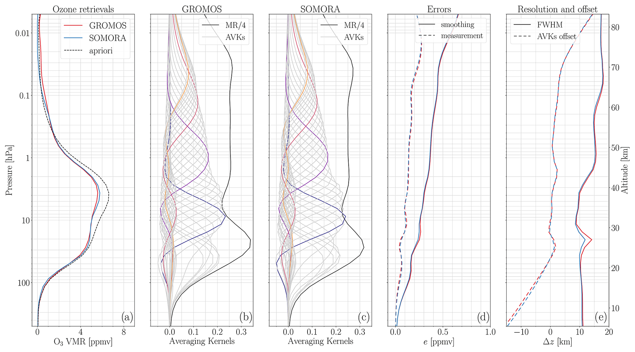
Figure 3 Example of GROMOS and SOMORA hourly ozone retrievals on 9 January 2017 around 14:30 UT with a tropospheric opacity τ≈0.4: panel (a) shows the a priori and retrieved ozone profiles, panels (b) and (c) show the GROMOS and SOMORA averaging kernels together with their MR (divided by 4 to fit in the same plots), panel (d) shows the smoothing and measurement error, and panel (e) shows the full width at half maximum (FWHM) and the offset between the AVKs peak and the actual altitude contribution. All quantities are retrieved on pressure levels, and approximated altitudes are indicated on the right. See the text for more details on each diagnostic quantity.

Figure 3 shows the corresponding ozone retrievals and main diagnostic quantities for the spectra shown in Fig. 2. It includes the averaging kernels (AVKs), which are a measure of the sensitivity of the retrieval to the true ozone profile at each pressure level. The sum of the AVKs at each level defines the measurement response (MR). It is an indication of the measurement contribution to the retrieved profile, whereas the remaining information comes from the a priori. In microwave remote sensing, a MR of 80 % is often used to define the lower and upper boundaries of the retrievals in order to limit the influence of the a priori on the results. Also included as diagnostic quantities are the smoothing and measurement errors computed by the OEM as defined by Rodgers (2000). The smoothing error is a consequence of the limited resolution of the instrument, whereas the measurement error arises from the noisy nature of the observations. Finally, we show the full width at half maximum (FWHM) of the AVKs at each level and the altitude offset (in kilometres) between the AVK maximum and its corresponding altitude. Both together give an indication on the altitude resolution and the vertical offset between the true and retrieved profiles.

3.3 Uncertainty budget

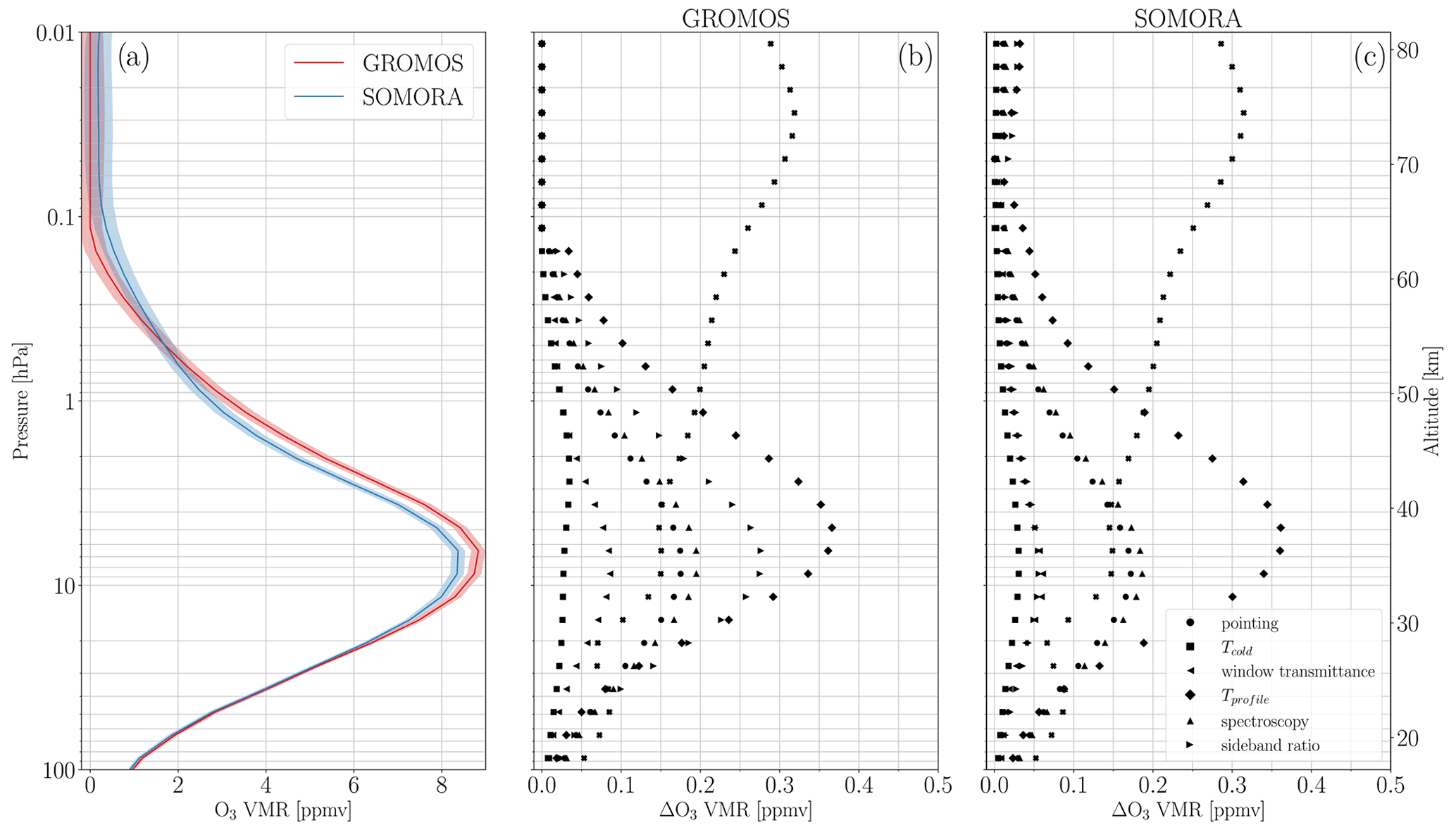
The retrieval errors presented above do not include systematic errors that can arise during the calibration or the retrievals. It is cumbersome to estimate all possible errors on such complex measurement setup and therefore, we decided to perform a sensitivity analysis on the most important error sources using two reference time periods with low (τ≈0.15) and high (τ≈1.3) atmospheric opacities. The uncertainties considered in our study are listed in Table 3 as well as the perturbations used for the sensitivity analysis. These were determined in different ways for each error source, deriving it either from measurement (e.g. T_cold, sideband ratio, window transmittance) or empirical values (e.g. pointing, spectroscopy).

Table 3 Potential error sources and the perturbations used for the sensitivity analysis.

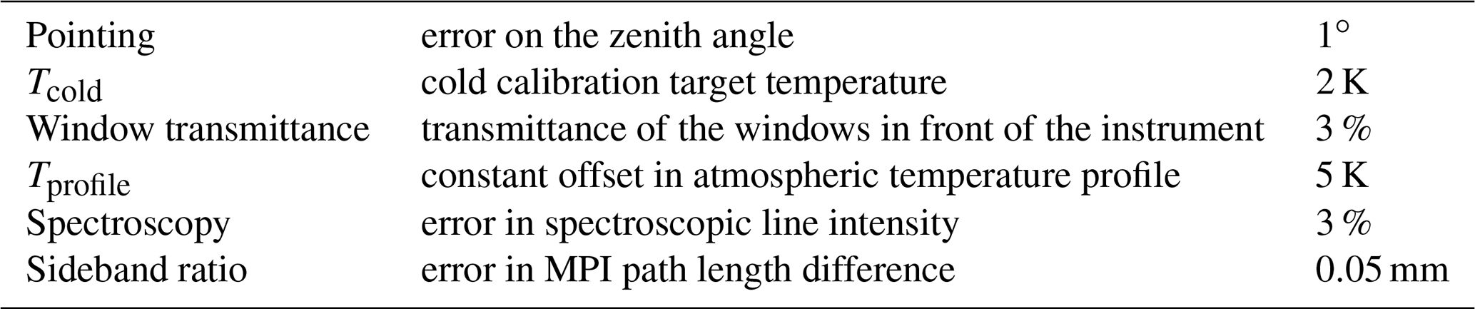
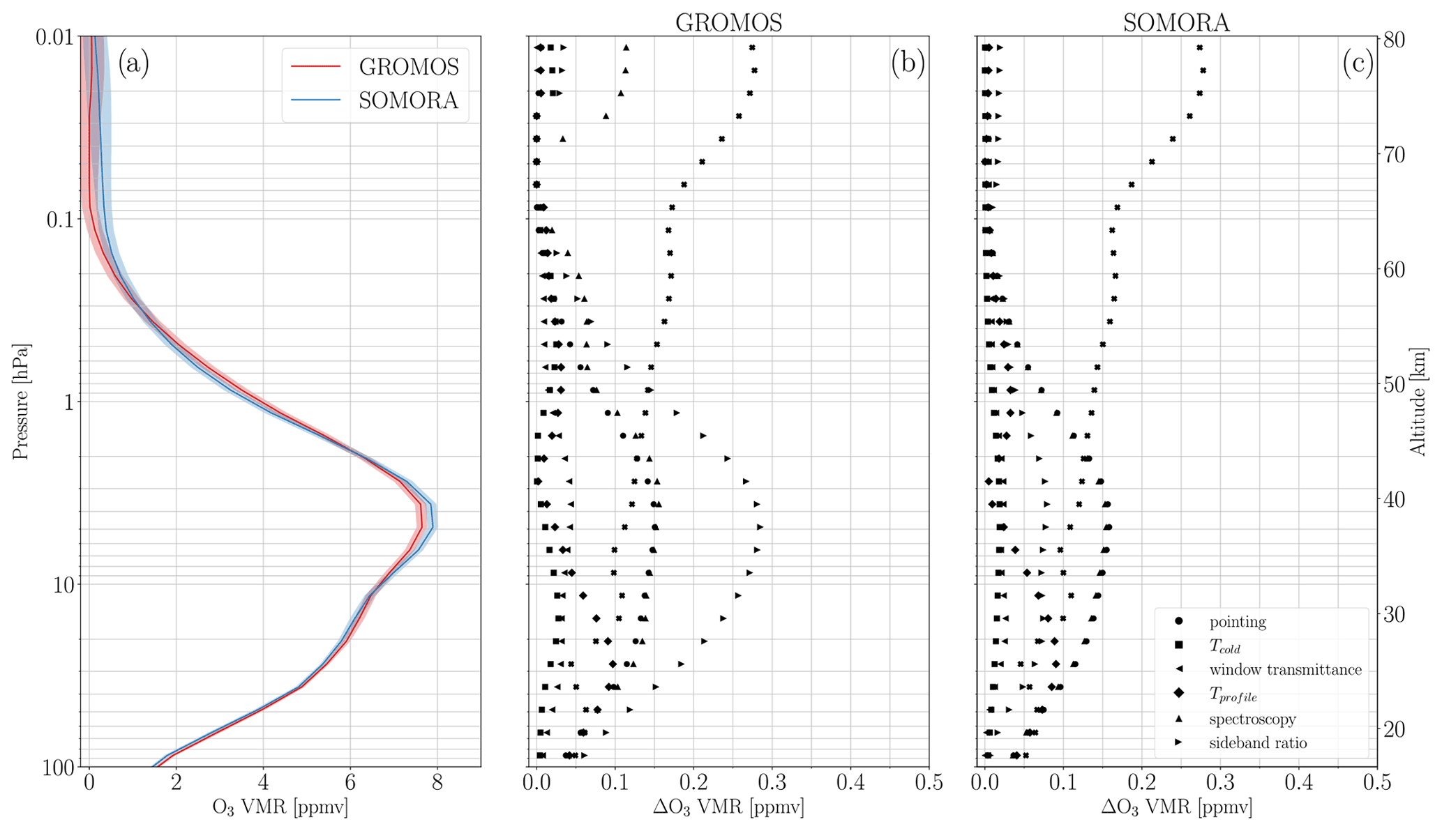
Figure 4 Uncertainty budget for GROMOS and SOMORA in a low-opacity case (τ≈0.15). Panel (a) shows the reference ozone profile chosen for the sensitivity analysis. Panels (b) and (c) show the ozone VMR uncertainties arising from the error sources listed in Table 3.

The uncertainty budget for GROMOS and SOMORA is presented in Fig. 4 in the case of low tropospheric opacities. The high-opacity cases for both instruments can be seen in Appendix B (Fig. B1).

In general, the sensitivity of GROMOS and SOMORA to the different perturbations is very similar. A notable exception is the higher sensitivity of GROMOS to the sideband path length, which is a consequence of its lower intermediate frequency. For both instruments, the total uncertainty is dominated by systematic errors below 2 hPa, whereas the measurement noise becomes quickly dominant above this point. In relative terms, the uncertainty is approximately 9 %–10 % for GROMOS and 7 %–8 % for SOMORA up to the stratopause and then increases significantly in the mesosphere.

In the case of high tropospheric opacity, the ozone emission line gets more attenuated by the tropospheric water vapour absorption. The AVKs get degraded, reducing the sensitivity of the retrievals and leading to higher uncertainties than at lower opacities. As can be seen in Fig. B1, the atmospheric temperature profile becomes the dominant contribution to the uncertainties below 1 hPa at higher opacity. This is likely due to the increased importance of the water vapour continuum retrieval, which is itself strongly dependent on tropospheric humidity and temperature. In the higher-opacity case, the total relative uncertainty in the stratosphere is 12 %–15 % for GROMOS and 10 %–12 % for SOMORA. In view of the perturbations and error sources considered in this study, these values compare well with similar ozone radiometers at other locations reported in the literature (e.g. Palm et al., 2010; Kopp et al., 2002).

4 Harmonized ozone time series

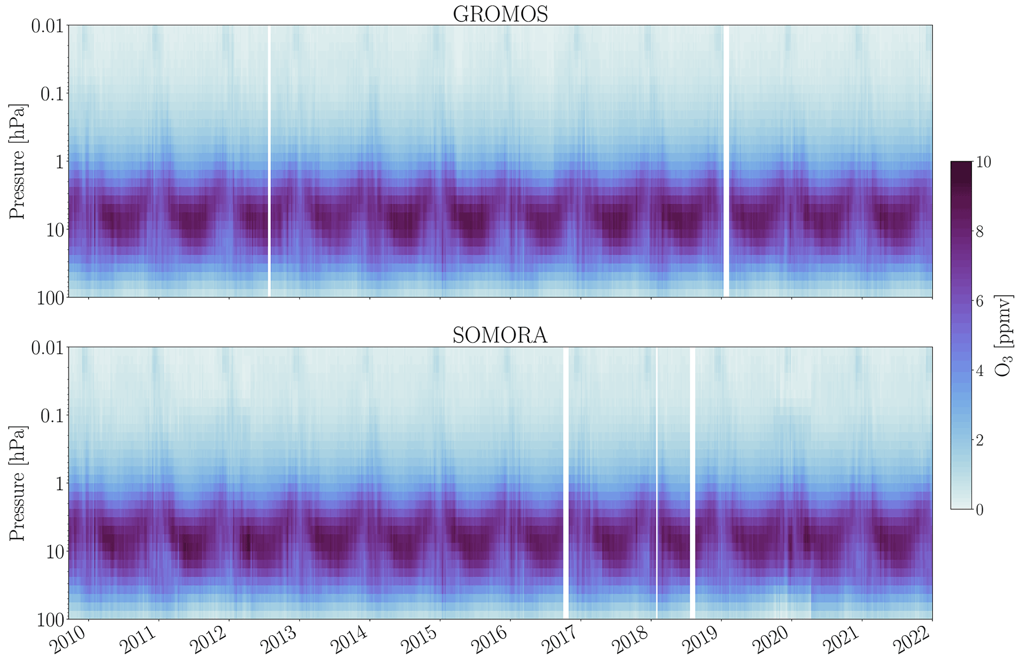
Using the new calibration and retrieval routines described previously, we have reprocessed the GROMOS and SOMORA data series for the time where they both use the AC240 spectrometer, i.e. from the end of 2009 until 2021. Figure 5 shows weekly averaged ozone profiles for GROMOS and SOMORA for the decade 2010–2020. It shows the consistency of the measurements and highlights the very few large interruptions happening on both instruments during this period. Most interruptions are due to instrumental issues (e.g. LN2 refilling or LO frequency stability) or atmospheric conditions (e.g. high tropospheric opacity masking the ozone emission line), and they usually last for a few hours at most. The longer interruptions result from cold load issues or hardware changes, which can last for a few days or weeks.

Figure 5 Weekly averaged ozone volume mixing ratio (VMR) profiles for GROMOS and SOMORA.

To validate these two data series, we first present a cross-comparison of the GROMOS and SOMORA data series and show the improvement resulting from the reprocessing compared to the previous retrieval version. We then compare both instruments against satellite-based ozone observations from MLS and SBUV above Switzerland.

4.1 Cross-comparison between GROMOS and SOMORA

GROMOS and SOMORA are located close to each other, have similar viewing directions, and experience similar tropospheric conditions during all seasons (Fig. A1). In addition, they have similar altitude range and sensitivity and can therefore be used for direct cross-validation of their time series. The upper panel in Fig. 6 shows the weekly mean relative differences between GROMOS and SOMORA harmonized data series (note that the lower panel of this figure will be discussed in Sect. 4.2). In general, GROMOS and SOMORA agree well in most of the middle atmosphere, with relative differences mostly lower than 10 % in the stratosphere and lower mesosphere (from ∼ 50 to 0.1 hPa), increasing towards lower and higher altitudes. The higher relative differences at lower and higher altitudes are partly explained by the shape of the ozone VMR profile when intensity is at its maximum in the stratosphere. In general, the lower altitudes are also the most impacted by instrumental baselines, which explains the increase in the differences below 50 hPa, whereas at higher altitudes the instrumental noise becomes the dominant factor and the sensitivity of the radiometers decreases quickly. In addition, the diurnal ozone variations typically become much larger in the mesosphere (e.g. around 20 % compared to a few percent in the stratosphere; Haefele et al., 2008).

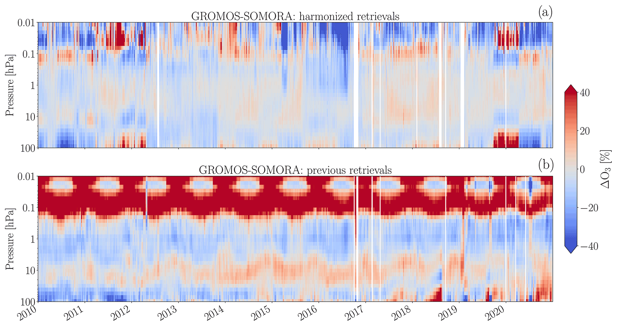
Figure 6 Weekly ozone relative difference between the new (a) and previous (b) GROMOS and SOMORA series.

Figure 7 Mean seasonal ozone VMR profiles (a) and their mean relative differences (b) and correlations (c). The shaded area in panel (b) indicates the ±10 % interval.

We also see some oscillatory patterns in the relative differences, some of which can be identified as clear seasonal patterns (e.g. in the lower stratosphere between 2014 and 2017). These seasonal differences are highlighted in Fig. 7, which shows seasonal ozone profile comparisons between GROMOS and SOMORA. The mean seasonal differences between the two instruments are lower than 10 % at all seasons and throughout most of the middle atmosphere and show a negative ozone bias from GROMOS in the upper mesosphere (p < 0.05 hPa). In the stratosphere and lower mesosphere, the ozone profiles are well correlated with Pearson's R coefficients mostly above 0.7 at most pressure levels and seasons (Fig. 7). However, this is not the case during summer, where we find significantly lower correlation between GROMOS and SOMORA ozone profiles.

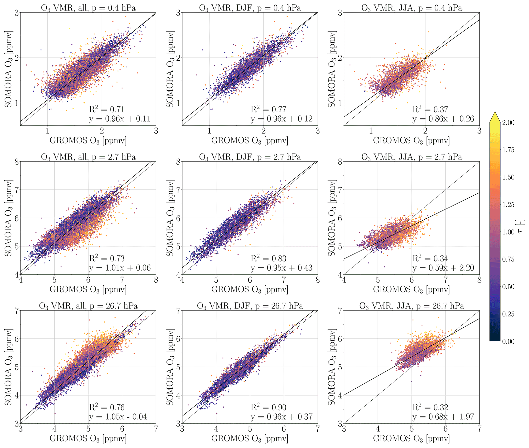
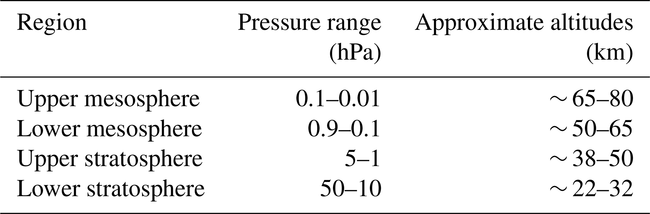
Figure 8 Mean ozone VMR for three different levels for the whole series (left column), the boreal winter season (middle column) and the boreal summer (right column). The three pressure levels correspond approximately to the lower stratosphere ($\mathrm{10}<p<\mathrm{50}$ hPa), upper stratosphere ($\mathrm{1}<p<\mathrm{5}$ hPa) and lower mesosphere ($\mathrm{0.1}<p<\mathrm{0.9}$ hPa). All data points are colour coded based on the atmospheric opacity (τ) computed at SOMORA measurement time and location. The linear regression coefficients and their coefficient of determination R² are indicated on each subplot.

Figure 8 shows scatter plots of their differences in three pressure level domains corresponding approximately to the lower stratosphere, the upper stratosphere and the lower mesosphere (see Table 4 for the definitions). It shows the net difference in atmospheric opacity between the winter and the summer and highlights the higher ozone variability during the wintertime. Figure 8 confirms the general good agreement between GROMOS and SOMORA in the middle atmosphere and corroborates the existence of a seasonal bias between the instruments during summertime.

Table 4 Definition of the pressure ranges and corresponding altitudes used in this study.

During the summertime, the warmer and wetter troposphere results in a higher opacity. This attenuates the ozone spectral line and thus decreases the retrieval sensitivity during summer. As discussed in Sect. 3.3, a higher tropospheric opacity also results in larger uncertainties in the retrieved ozone profile. In case of very hot and humid conditions, the troposphere can become optically thick at 142 GHz, which can prevent the retrieval of ozone profiles. It can be seen in Fig. A1, which shows higher tropospheric opacity in summertime than during the other seasons. However, Fig. A1 also shows that the difference in tropospheric opacity at the two sites remains constant, independent of the season. In addition, we investigated the correlations between GROMOS and SOMORA considering only profiles measured at low tropospheric opacity (τ⩽1) and did not see any significant changes in the results. For these reasons, we believe that the summer bias does not result from the higher tropospheric opacities affecting this season.

The reasons for the summer seasonal bias remain unclear, but we assume that they result from seasonal temperature and humidity cycles in the troposphere. Indeed, despite controlled room temperature for both instruments, the higher summer temperatures still influence the room and window temperatures and consequently the instruments (e.g. receiver noise temperature or instrumental baselines). We believe that the hardware components of GROMOS and SOMORA have different sensitivity to such influences, which could explain the seasonal patterns observed in their relative differences and the lower correlation of the ozone profiles during summer.

In addition to these seasonal effects, Fig. 6 highlights some sudden changes in the differences between the two instruments, most of which can be related to a specific instrumental issue on either instrument. It can be seen for instance in April 2012, where the cold load observation angle was changed on SOMORA, reducing its baseline significantly. Another example is the strong negative ozone differences during summer 2016, which were due to a frequency lock problem in GROMOS. Finally, the large flagged period starting at the end of 2019 marks the beginning of several instrumental issues on SOMORA that were finally solved by the replacement of the LO baseband converter in September 2020. All of these issues have been identified and documented and are flagged accordingly in the new ozone data series. A detailed documentation of the time series can be found together with the data.

4.2 Comparison with previous retrievals

Computing trends for GROMOS and SOMORA is out of scope of this contribution but we would still like to provide some first elements toward answering whether this harmonization can help solving the discrepancies previously found between both instruments (Bernet et al., 2019; Petropavlovskikh et al., 2019). Therefore, we compare our new harmonized ozone time series with the previous data version of GROMOS and SOMORA.

Figure 6 shows the weekly relative differences between the new harmonized series (upper panel) and the previous retrievals (lower panel) from 2010 to 2021. It highlights the significant improvements introduced by the harmonization process in most of the pressure range covered by the radiometers. Among other changes, it corrects the strong positive ozone bias from GROMOS seen in the mesosphere and reduces the stratospheric ozone difference clearly visible in many years of the previous data series at ∼ 10 hPa. The differences between the previous series also showed a quite strong seasonal signal. As the previous processing was different between the two instruments, in particular in the way it was treating the tropospheric attenuation, it gives some confidence that the remaining seasonal bias in the new series is not an artefact introduced by the new retrieval method.

Although the harmonized retrievals improve most of the time period considered, it seems that the problems seen on SOMORA in 2020 are less well treated in the new processing. Indeed, in the previous processing the sine baseline periods were adapted daily during this time whereas the new processing only considered fixed periods. It indicates that the instrumental baselines on SOMORA varied significantly during this period and highlights the need to treat it carefully for further analysis.

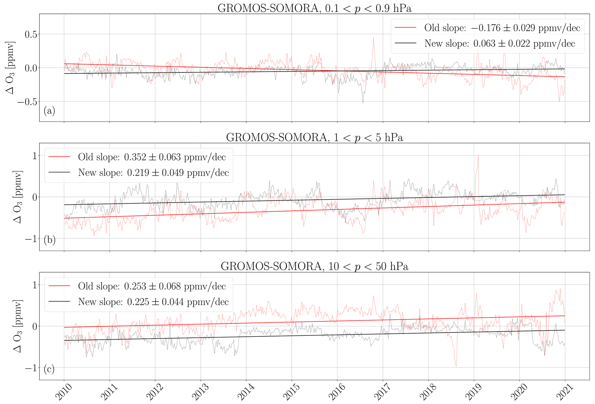
Figure 9 Weekly ozone differences between the previous and the new GROMOS and SOMORA series for the three pressure levels defined in Table 4: (a) lower mesosphere, (b) upper stratosphere and (c) lower stratosphere. A linear fit of the differences is shown as a straight line for the previous and the new series. The slope values are indicated with a 95 % confidence interval.

From Fig. 6, it is clear that the harmonized processing significantly reduces the differences between the GROMOS and SOMORA ozone time series. However, the question remains if it can solve the discrepancies found between their respective trends. Of course, the full reprocessing of the series (including the decade 2000–2010) would be needed to fully answer this question, but we present some preliminary results showing the temporal evolution of the ozone differences between both series in Fig. 9. It shows the weekly mean differences between GROMOS and SOMORA with the previous and new retrieval algorithms in three pressure ranges. Ideally, these differences should be constant to guarantee similar trends from both instruments. Simple linear regressions have been performed on these data and indicate smaller drift intensities at all pressure ranges from the new data processing that are significant above 10 hPa.

As a consequence, the future trends to be derived for this decade from the new series should be in better agreement than with the previous retrievals. However, even with the new series, we still observe a drift between both instruments in the stratosphere, which calls for a careful treatment of spurious data periods for the next trends analysis, as done in Bernet et al. (2021).

5 Comparison with satellites

Attention was paid to keep GROMOS and SOMORA data processing fully independent. However, they would be both impacted by any bias introduced by the calibration or retrieval algorithms and therefore, we provide further validation by comparing their observations with satellite measurements.

5.1 Aura MLS

As the main validation dataset, we use ozone measurements from the Microwave Limb Sounder (MLS) on the Aura satellite launched in 2004 (Waters et al., 2006). It is operated by the National Aeronautics and Space Administration (NASA) in the frame of the Earth Observing System and has been used extensively for ozone profile validation over many regions and against many other observing systems (e.g. Boyd et al., 2007; Livesey et al., 2008; Hubert et al., 2016).

MLS is a passive microwave radiometer observing the ozone emission line around 240 GHz in a limb sounding geometry. It follows a sun-synchronous orbit which results in two overpasses per day around 01:00 and 13:00 UTC​​​​​​​ over central Europe. In this work, we have used the latest level 2 ozone retrievals (version 5) and the recommended data screening described in Livesey et al. (2022). It results in ozone VMR profiles between 261 to 0.001 hPa with a typical vertical resolution ranging from ∼ 2.5 km in the lower stratosphere increasing to ∼ 5.5 km at the mesopause with an accuracy of 5 %–10 % in the stratosphere increasing up to 100 % at 0.01 hPa.

For the following comparisons, we extracted co-located MLS observations to GROMOS and SOMORA. As spatial coincidence criteria, we use ±3.6^∘ in latitude and ±10.5^∘ in longitude from Bern, an area corresponding approximately to Central Europe. As temporal criteria, we averaged the MWR and the MLS profiles within 3 h time windows and keep only the time windows where both MLS and the MWR have profiles with sufficient data quality.

The MLS vertical resolution of ozone retrievals is much lower than the one from the MWRs. It means that the MWRs will essentially observe a smoothed vertical profile compared to the MLS observations. Therefore, the higher-resolved MLS profiles are convolved with the MWR averaging kernels for the comparisons (see Connor et al., 1994; Tsou et al., 1995). This AVKs smoothing also enables the removal of the influence of the a priori and follows Eq. (1):

$$\begin{array}{}\text{(1)}& {\mathit{x}}_{\mathrm{c}}={\mathit{x}}_{\mathrm{a}}+\mathbf{A}(\mathit{x}-{\mathit{x}}_{\mathrm{a}}),\end{array}$$

where x is the higher-resolution profile (MLS), x_a is the a priori profile from the MWR retrievals, A are the averaging kernels and x_c is the resulting convolved profile.

5.2 SBUV/2

In addition to MLS, we also use the latest release of the Solar Backscatter Ultraviolet Radiometer (SBUV/2) Merged Ozone Dataset (MOD) (Frith et al., 2020; Ziemke et al., 2021). This dataset provides daily overpasses over many ground-based ozone measurement stations, including Payerne in Switzerland. It provides stratospheric ozone VMR profiles from 50 to 0.5 hPa merged according to the new MOD v2 Release 1 derived from SBUV and adjusted for the diurnal cycles to an equivalent local measurement time of 13:30. The vertical resolution from the SBUV retrievals is ∼ 6–7 km in the middle and upper stratosphere (McPeters et al., 2013; Bhartia et al., 2013), which is closer to the vertical resolution of GROMOS and SOMORA in this region. For this reason, contrary to MLS, we do not apply any AVK smoothing to the SBUV measurements for the following comparisons.

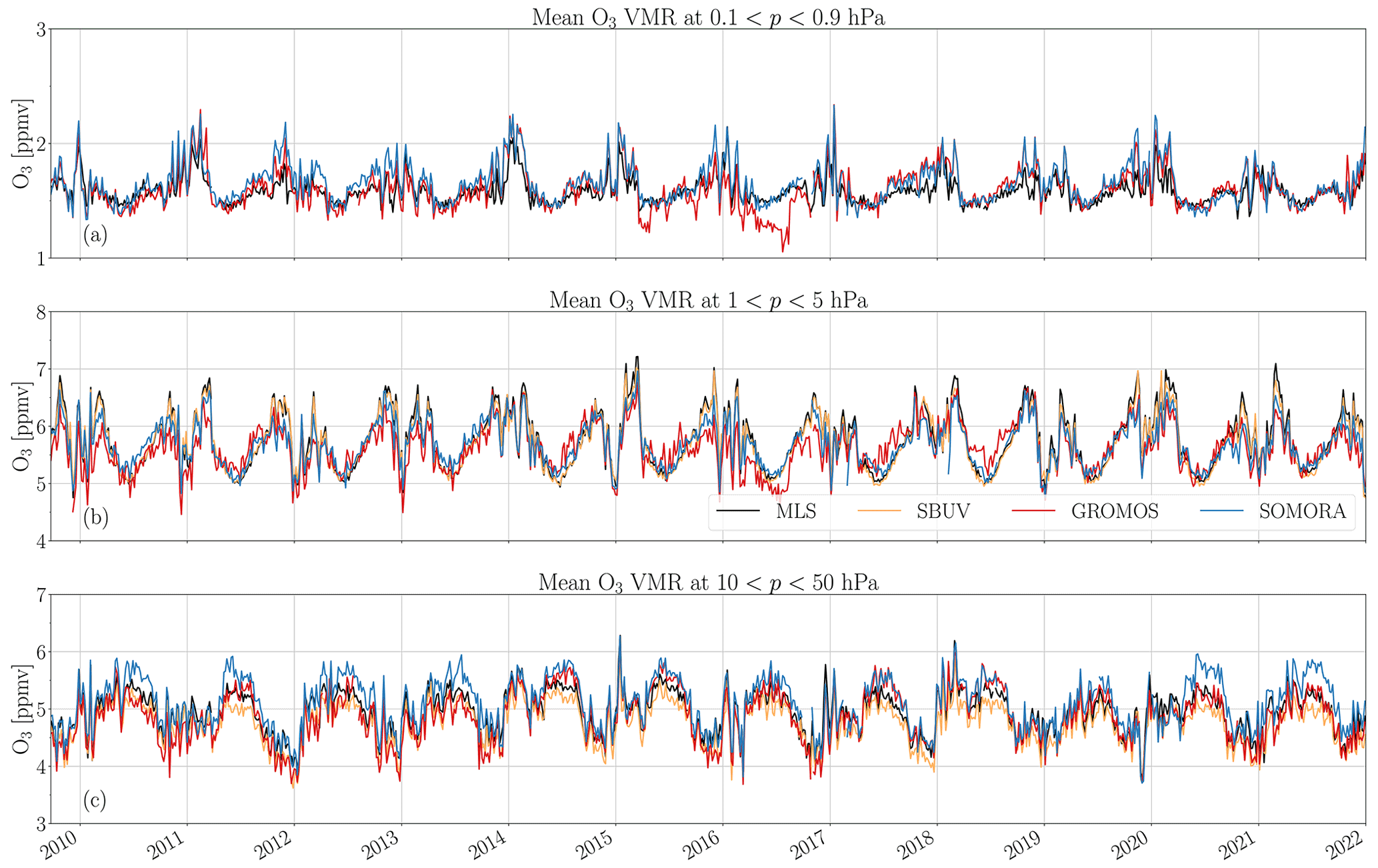
Figure 10 Weekly averaged ozone VMR from MLS, SBUV, GROMOS and SOMORA at three pressure intervals: (a) lower mesosphere, (b) upper stratosphere and (c) lower stratosphere. The SBUV dataset extends only up to 0.5 hPa and is therefore not shown in panel (a).

5.3 Time series

Figure 10 shows weekly averaged GROMOS and SOMORA time series together with SBUV and MLS measurements on three pressure ranges corresponding to the lower stratosphere, upper stratosphere and lower mesosphere. It shows the consistencies of the GROMOS and SOMORA time series and highlights the good agreement of both MWRs with both satellite datasets during the last decade. As these time series are already averaged on given pressure ranges, we did not apply any AVK smoothing on the MLS data at this stage. It is also important to keep in mind that the SBUV daily dataset is adjusted to daytime (13:30), whereas both MLS and the MWRs have both daytime and night-time measurements.

In the stratosphere, clear seasonal patterns are well captured by all datasets, and the higher winter ozone variability is clearly visible at all pressure levels. On timescales of a few weeks, we can see that all four datasets are able to capture the larger ozone variations well not only in the stratosphere but also in the mesosphere where these variations become relatively small compared to the amplitude of the ozone diurnal cycle.

We can see a slight bias of the SOMORA data series in the lower stratosphere. It is especially visible before 2014 and after 2019, as has been mentioned previously. This plot also helps to identify some remaining spurious time periods in the new harmonized series (e.g. GROMOS data in summer 2016). From a qualitative point of view, we do not observe large drifts from any of the datasets with respect to the others. More work will be needed to confirm the stability from both MWRs, but it gives some confidence that both instruments can be used for trends analysis in the decade 2010–2020.

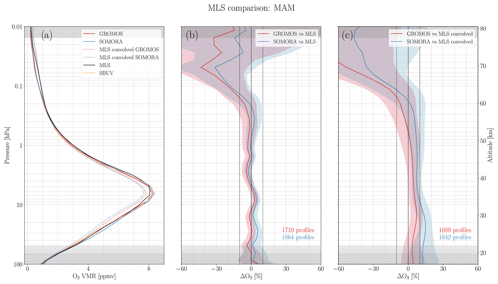
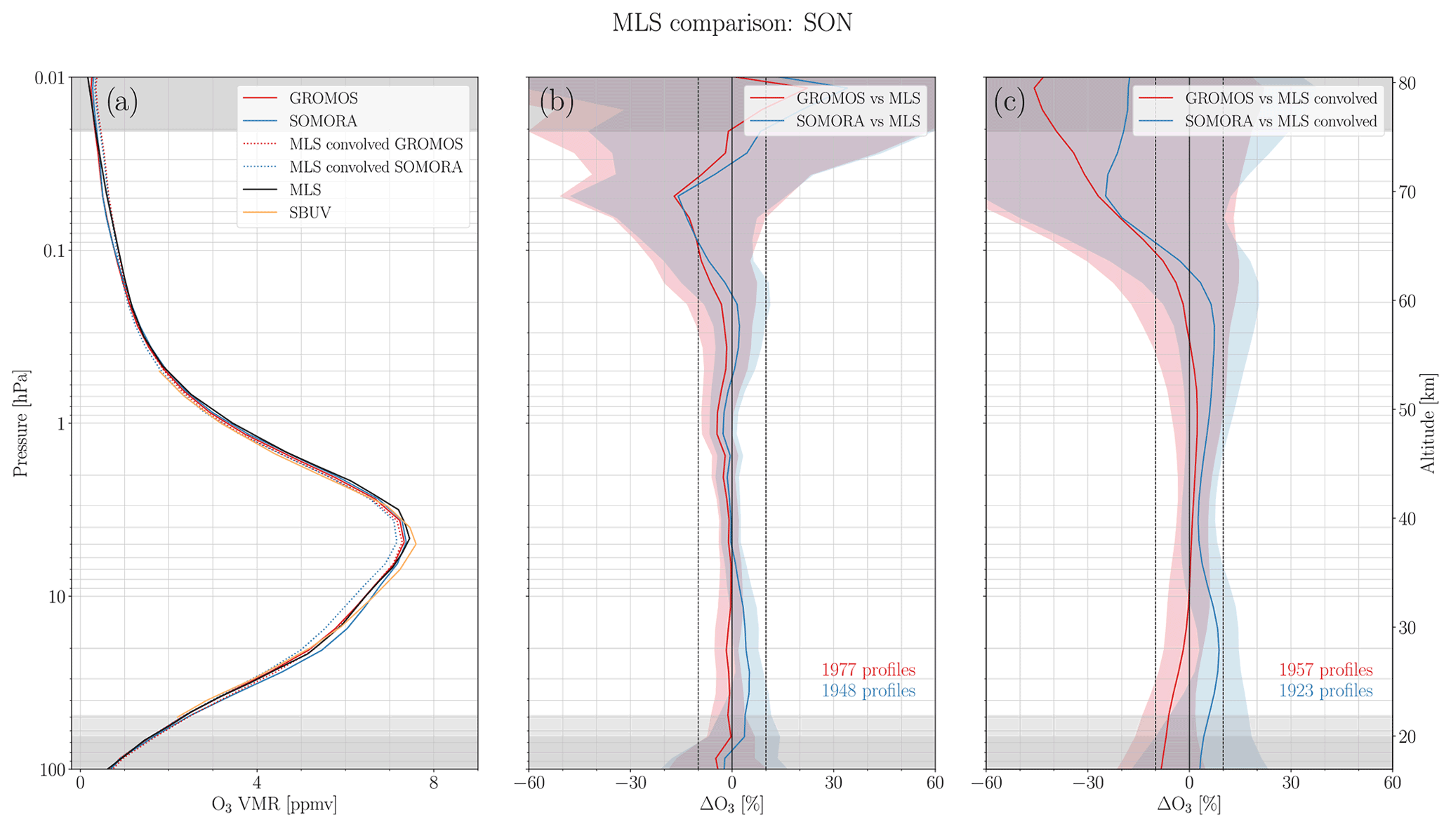
5.4 Profile comparisons

As quantitative validation, we show seasonal comparisons of MWRs profiles with the satellite datasets. In the following, we mostly focus on the MLS time series because it covers the same altitude range as the MWRs and because SBUV only provides daytime measurements. For the period between 2009 and 2021, we obtain more than 7100 co-located profiles between MLS and each MWR, giving approximately 1700 profiles per meteorological season. Figures 11 and 12 show comparisons between winter (resp. summer) ozone profiles measured by GROMOS, SOMORA, SBUV and MLS. Both figures show the mean seasonal ozone profile from each dataset and the relative differences between MLS and the MWRs with and without AVK convolution. The comparisons for spring and autumn are shown in Appendix C (Figs. C1 and C2).

Figure 11 Seasonal comparison with MLS and SBUV during winter months (December, January and February). Panel (b) shows the relative differences with MLS, whereas panel (c) shows the relative differences with the convolved MLS profiles. The coloured areas show the standard deviation of the differences with MLS, and the grey shading indicates the limits where the a priori contribution exceeds 20 %. The dashed vertical lines indicate the ±10 % interval.

Figure 12 The same as Fig. 11 but for summer (June, July and August).

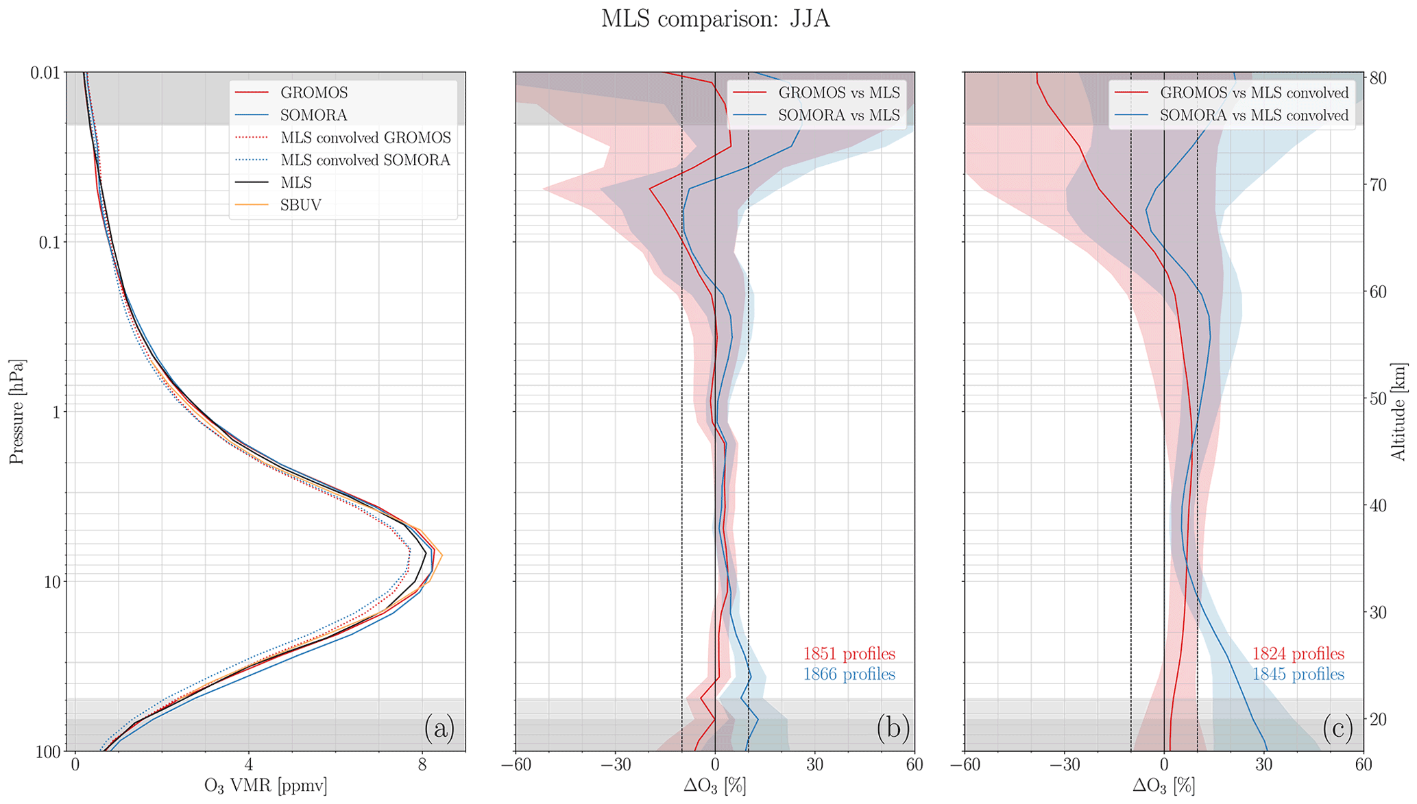
Table 5 Mean relative VMR differences ((MWR − MLS) $/$ MWR) between MWRs and MLS at three pressure ranges, with and without AVK convolution. In parentheses we show the standard deviations of the VMR relative differences in each pressure range.

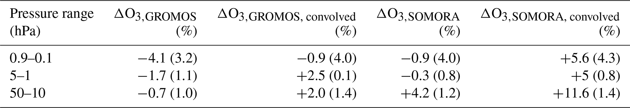
Both GROMOS and SOMORA show very good agreement with MLS at all seasons and altitudes, with the exception of SOMORA during summertime. Mean seasonal relative differences between the two instruments and co-located MLS profiles are within 10 % in the stratosphere and lower mesosphere (up to ∼ 60 km), corresponding to the expected uncertainties of the MWRs. Above in the mesosphere, the relative differences between the MWRs and MLS grow rapidly and show some oscillations. For most of the mesosphere, the mean seasonal relative differences stay below 50 % for both instruments, but given the errors reported for the MWRs and MLS at these altitudes, we will focus our discussion on the region from ∼ 20 to 60 km. The relative differences with SBUV (not shown) are very similar to those with MLS and are below 10 % in the whole stratosphere for the two instruments.

Figure 12 again reveals the summer bias mentioned previously. Taking MLS as a reference, this plot indicates that the summer bias in the lower stratosphere is the result of an overestimation of ozone by SOMORA during this season. The reason for this could be a seasonal change in the instrumental baselines that is not taken into account in the retrieval. For both instruments, the differences with the convolved MLS profiles are still smaller in autumn and winter than in spring and summer when the absorption by the troposphere is stronger.

Moreira et al. (2017) compared the previous GROMOS retrieval dataset to MLS between 2009 and 2016. Similar agreement was found in the middle stratosphere; however, this quickly degraded at lower and higher altitudes. This is in accordance with the results shown in Fig. 6 and confirms the improvement brought by the new data processing. SOMORA showed similar agreement with MLS in the range 25 to 0.1 hPa between 2004 and 2015 (Maillard Barras et al., 2020). Below 25 hPa, SOMORA showed a positive bias compared to other datasets that gives confidence that this bias is not related to the new data processing.

Similar comparisons between MWR and MLS has been performed at various locations (e.g. Boyd et al., 2007; Palm et al., 2010; Ryan et al., 2016) and showed similar results to the ones obtained in our study. This is confirmed by the mean ozone VMR relative differences between MWR and MLS given in Table 5 for the middle atmosphere. Averaged over these pressure ranges and the entire time period, the differences between MLS and the MWRs are less than 5 % in the stratosphere and lower mesosphere.

Overall, SOMORA and GROMOS profiles are in better accordance with the non-convolved MLS than with the convolved MLS profiles. This can be seen for both instruments and at the three pressure ranges from the seasonal plots and in Table 5. It is not entirely clear why these differences are larger with the convolved MLS profiles, but it does not result from sampling differences (not shown). As it seems especially visible in SOMORA in the lower stratosphere, it could potentially arise from instrumental baselines impacting the AVKs.

6 Conclusions

New harmonized data series from two Swiss ozone ground-based microwave radiometers are now available from 2009 to 2021. The reprocessing provides a full harmonization at all levels, from the calibration of the raw data to the retrieval of the ozone profiles. It includes the data inputs and outputs, the systematic flagging, the output temporal resolution and the retrieval grids. The harmonization makes the comparison and the identification of biases easier than in the past. It significantly improves the agreement between the two instruments in this time period and reduces the long-term drift of their differences. It should help to resolve the discrepancies previously found in the trend estimates derived from these two time series.

However, despite these significant improvements, systematic differences remain between the two instruments. They include a seasonal bias, mostly visible in the lower stratosphere in summer, as well as a negative ozone bias of GROMOS in the upper mesosphere. Further work is needed to fully understand these systematic biases but they probably both arise from instrumental sources as they were already seen in the previous retrieval versions. In addition, limited anomalous time periods still remain on both instruments but most of their causes are now identified and documented. The new harmonized data series are also compared against two independent and co-located satellite datasets. Both instruments show a good agreement with SBUV and MLS, with mean relative differences below 10 % in most of the stratosphere and lower mesosphere (up to ∼ 60 km).

The new retrieval products of ozone profiles at Bern and Payerne are available and will be submitted to NDACC. We also plan to extend the harmonization process to the older observations from these two instruments in order to provide the full harmonized ozone time series since 1994 (GROMOS) and 2000 (SOMORA). The collocation of two harmonized time series with high temporal resolution also opens the way to unique short-term ozone variations analyses.

Appendix A: Opacities

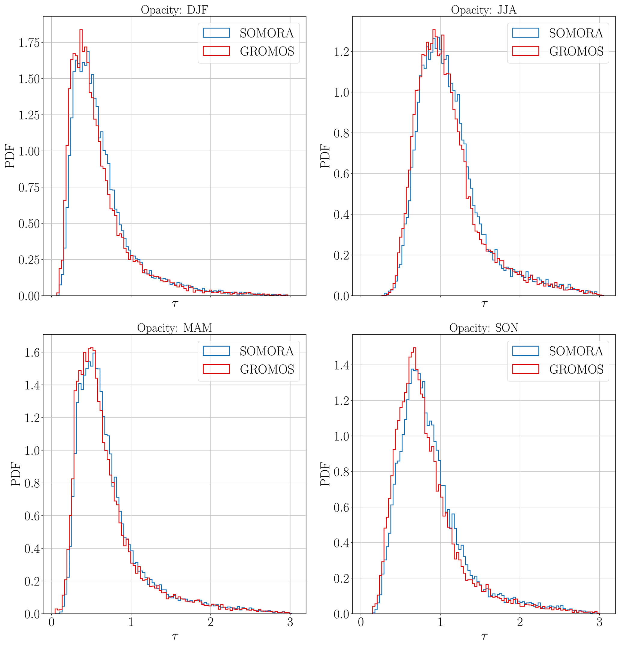
Figure A1 Seasonal comparisons of hourly tropospheric opacities in Bern (GROMOS) and Payerne (SOMORA) from 2009 to 2021.

Appendix B: Uncertainty budget at high atmospheric opacities

Figure B1 Uncertainty budget for GROMOS and SOMORA in the high-opacity case (τ≈1.3). Panel (a) shows the reference ozone profile chosen for the sensitivity analysis. Panels (b) and (c) show the ozone VMR uncertainties arising from the error sources listed in Table 3.

Appendix C: Seasonal comparison with MLS and SBUV

Figure C1 The same as Fig. 11 but for spring (March, April and May).

Figure C2 The same as Fig. 11 but for autumn (September, October and November).