the Creative Commons Attribution 4.0 License.
the Creative Commons Attribution 4.0 License.
 | 04 Jan 2023
True eddy accumulation – Part 1: Solutions to the problem of non-vanishing mean vertical wind velocity
Lukas Siebicke
The true eddy accumulation (TEA) method provides direct measurements of ecosystem-level turbulent fluxes for a wide range of atmospheric constituents. TEA utilizes conditional sampling to overcome the requirement for a fast sensor response demanded by the state-of-the-art eddy covariance (EC) method.
The TEA method is formulated under the assumption of ideal conditions with a zero mean vertical wind velocity during the averaging interval. However, this idealization is rarely met under field conditions. Additionally, unlike in EC, this assumption cannot be imposed in post-processing due to the real-time nature of sampling and the absence of high-frequency measurements of the scalar. Consequently, fluxes measured with the TEA method are biased with a non-turbulent advective term that scales with the scalar mean concentration.
Here, we explore the magnitude of this biased advective term and potential ways to minimize or remove it. We propose a new formulation to calculate TEA fluxes that minimizes the bias term. The new formulation shows that the magnitude of the error is constrained to when the stationarity criterion is fulfilled. Here, w is the vertical wind velocity, and the overbar denotes time averaging. The error is shown to be dependent on the asymmetry of atmospheric transport, represented by the coefficient αc. Two methods of estimating the coefficient αc are proposed: a probabilistic treatment of turbulent transport and a method utilizing the assumption of scalar similarity. We show how other formulas for calculating the TEA flux are linked to the new formulation and explore the different corrections in a numerical simulation.
The new formulation avoids the direct dependence of the bias term on the scalar background concentration. This result increases confidence in applying the TEA method to measuring fluxes of atmospheric constituents. This is particularly relevant to scalars with a large background concentration and a small flux. This paper is Part 1 of a two-part series on true eddy accumulation.
- Article
(1613 KB) - Full-text XML
- Companion paper
- BibTeX
- EndNote


Micrometeorological methods provide noninvasive, in situ, integrated, and continuous point measurements for ecosystem fluxes on a scale ideal for ecosystem study (Baldocchi et al., 1988; Baldocchi, 2014). Among micrometeorological methods, eddy covariance (EC) has become the de facto method for measuring ecosystem fluxes for the past 40 years. The EC method is the most direct micrometeorological method. It is also relatively easy to set up and operate. These features have led to the wide use and adoption of the EC method at hundreds of sites worldwide, including several regional and global flux measurement networks such as ICOS and FLUXNET (Hicks and Baldocchi, 2020).
The EC method depends on the fast measurement of vertical wind velocity and the scalar concentration (such as an atmospheric constituent). The requirement for fast measurement frequency (10 to 20 Hz) limits the application of the method to a handful of atmospheric constituents for which fast gas analyzers are available. Alternative methods that work for slow gas analyzers include (i) signal downsampling methods (Lenschow et al., 1994), such as disjunct eddy accumulation (H. J. I. Rinne et al., 2000; Turnipseed et al., 2009) and disjunct eddy covariance (Rinne and Ammann, 2012), and (ii) indirect methods such as flux gradient methods (e.g., J. Rinne et al., 2000) which depend on the Monin–Obukhov similarity theory (Monin and Obukhov, 1954) and relaxed eddy accumulation (REA) which assumes flux-variance similarity (Businger and Oncley, 1990). The true eddy accumulation (TEA) method (Desjardins, 1977) is the most direct and mathematically equivalent alternative to eddy covariance among accumulation methods. Unlike EC, the TEA method requires the concentration measurements to be carried out once every averaging interval (30 min) (Businger and Oncley, 1990). The TEA method is formulated under ideal conditions assuming a zero mean vertical wind velocity during the averaging interval. This assumption is almost never met under field conditions, and it is not possible to enforce in post-processing due to lacking high-frequency information on the scalar concentration. As a result, the non-vanishing vertical mean velocity will contribute to a systematic error in the flux. Nonzero mean vertical wind velocity is a source of error for all eddy accumulation methods, including TEA (Hicks and McMillen, 1984), relaxed eddy accumulation (REA) (Pattey et al., 1993; Businger and Oncley, 1990; Bowling et al., 1998), and disjunct eddy accumulation (DEA) (Turnipseed et al., 2009). The reported bias in the flux due to nonzero varies with different studies and accumulation methods. For TEA, Hicks and McMillen (1984) recommended that should not exceed 0.0005 σw if accumulated mass is measured and 0.02 σw when concentrations are measured directly. Turnipseed et al. (2009) reported that a mean vertical wind bias of ± 0.25 σw leads to a ± 15 % mean systematic bias in the flux using the disjunct eddy accumulation method. Values reported for the REA method show a systematic bias of approximately 5 % of the flux due to a of 0.20 σw (Pattey et al., 1993), which agrees with the recommendations of Businger and Oncley (1990). The magnitude of the residual mean vertical velocity depends on the meteorological and topographic features of the measurement site and is larger at complex sites (Rannik et al., 2020).
In this paper, we revise the theory of the true eddy accumulation method and obtain a generalized equation that isolates the error due to nonzero vertical wind velocity. The new equation shows that the error in the flux is a function of the atmospheric transport represented by the transport asymmetry coefficient, αc. We study the value and the interpretation of this coefficient in the framework of quadrant analysis and define its boundary conditions. Next, we show analytical and empirical ways to obtain the transport asymmetry coefficient and explore the implications of these estimates for the flux in a numerical simulation. Finally, we show how existing formulations for calculating the TEA flux are special cases of the new equation.
2.1 Eddy covariance
The net ecosystem exchange (NEE) of a scalar c (such as an atmospheric constituent) is the total vertical flux across the measurement plane at a height h and the change in storage below that height (Gu et al., 2012):
where w is the vertical wind velocity (m s−1), and c is the molar density (mol m−3) of the scalar of interest (such as CO2). The previous equation can be reached either from a holistic mass balance approach or by averaging the continuity equation for the scalar c and integrating from the surface to measurement height h. In both cases, horizontal advection is ignored as a virtue of the assumption of horizontal homogeneity, and molecular diffusion is ignored due to its small magnitude (Gu et al., 2012). For a full discussion on the equations of surface flux, see, for example Finnigan et al. (2003) and Foken et al. (2012a).
The storage term measurements and value are beyond the scope of this study, and therefore we ignore them. Consequently, the total vertical flux is represented by the first term on the right-hand side of Eq. (1), which can be further decomposed into turbulent and mean advective parts.
The overlines denote ensemble averages that obey Reynolds averaging rules. Primes represent departures from the mean. The ensemble averages are estimated experimentally by time averages. Thus, for a stationary time series drawn from an ensemble, the turbulent flux for the averaging period, Δt, can be written as
where w(t) and c(t) are realizations of the vertical wind velocity and the scalar quantity such as CO2 concentration, respectively.
2.2 True eddy accumulation
The true eddy accumulation method circumvents the need to record the fluctuations of scalar concentration at a frequency sufficient to represent the individual flux transport eddies. Instead, it is sufficient to measure the mean product for updraft and downdraft once for each averaging interval, Δt (e.g., 30 min).
The product of w and c is realized by physically collecting air samples with a flow rate proportional to the vertical wind velocity, w. The method is formulated assuming ideal conditions in which the mean vertical wind velocity during the averaging period is assumed to be zero. When , the second term on the right-hand side of Eq. (2) will be zero and the turbulent flux will equal the total ecosystem flux . By separating depending on the direction of the vertical wind velocity we can write
Hence, by sampling air with a flow rate proportional to the magnitude of vertical wind velocity and accumulating it according to its direction in updraft and downdraft reservoirs, one can measure the quantity and consequently the flux without having to measure the high-frequency fluctuations of the scalar, c (Desjardins, 1977; Hicks and McMillen, 1984).
Sampling air proportional to the magnitude of vertical wind velocity requires a scaling parameter, A, that ensures the proportionality of the flow rate to the magnitude of vertical wind velocity. The scaling parameter is the product of the pump calibration coefficients and other coefficients used to adjust the system's dynamic range. For a short interval of time dt, a sample of the volume will be collected in the system. The accumulated sample volume in each of the two reservoirs during a long enough averaging period Δt (30 to 60 min) will be
By the end of the averaging period, Δt, the flux will be equal to the difference in the scalar accumulated mass between updraft and downdraft reservoirs.
If it is desired to formulate the flux in terms of the accumulated scalar concentration (mol m−3) instead of the accumulated mass, the average scalar density of accumulated samples in each of the reservoirs will equal the accumulated mass of the scalar divided by the accumulated volume:
where Cacc is the accumulated scalar density and the arrows indicate the reservoir. The measured concentration in Eq. (7) is the weighted mean of the scalar concentration and the magnitude of the vertical wind velocity.
When is assumed to be zero, , and we can write the flux in terms of concentrations of accumulated samples, similar to Hicks and McMillen (1984):
where is the mean of the magnitude of the vertical wind velocity.
2.3 The problem of nonzero mean vertical wind
Although the total ecosystem flux is defined to be in Eq. (2), it is not possible to directly use the measured w and c to calculate the total flux. The reason is the difficulty of obtaining an accurate measurement of w. Any non-turbulent offset (bias) in the mean vertical velocity will lead to a flux biased with . Several factors contribute to a biased mean vertical wind velocity including topography at particular in complex sites, non-alignment of the anemometer with local topography, biases in anemometers, flow perturbations, and meteorological factors induced by local circulation or topographical drainage (Lee et al., 2005; Paw U et al., 2000; Heinesch et al., 2007). Therefore, the measured biased advective term needs to be discarded and the true physical term, known as the “Webb term” or Webb–Pearman–Leuning (WPL) term, needs to be estimated by other means (Webb et al., 1980; Fuehrer and Friehe, 2002). The original formulation of the TEA method assumes a zero mean vertical wind velocity during the flux averaging interval and thus assumes the total ecosystem flux to be equal to the turbulent flux, . However, this assumption is rarely valid under field conditions for the reasons outlined earlier, and the measured TEA flux will be a biased total vertical flux, . If the turbulent flux is to be measured using the TEA method, the biased term needs to be removed.
Previous efforts have been focused on minimizing to reduce the bias in the TEA flux. However, since the wind information cannot be changed after sampling, any treatments for the wind velocity measurements are final when the air samples have been collected. Thus, there is no way to guarantee a zero mean vertical velocity. A common approach to nullifying mean vertical wind velocity in EC measurements is to rotate the wind coordinates in post-processing to force to zero for each averaging interval. This method – commonly referred to as double rotation – is not feasible in eddy accumulation methods. The planar fit method (Wilczak et al., 2001) and its variants, such as the sector-wise planar fit (Foken et al., 2004), are better suited for online application in the TEA method (Siebicke and Emad, 2019).
The planar fit method aligns the sonic coordinates with the long-term streamline coordinates by aligning the wind vector with the plane that minimizes the sum of squares of the vertical wind velocity means for a long period of time (weeks to months). This approach, while minimizing the vertical wind velocity means of the individual averaging intervals, does not force them to be zero. Considerable spread of values around zero can still be observed after applying the planar fit method (Sun, 2007; Rannik et al., 2020).
2.4 TEA equation under nonzero conditions
The goal here is to enable measuring the turbulent flux from TEA measurements when . The key to extending the TEA equation to conditions of nonzero is to obtain an estimate of the scalar mean from TEA measurements and consequently remove the biased advective term . We achieve this by using the weighted mean of c and as an estimate for c after correcting for the correlation between them.
The weighted mean of the scalar, c, and the vertical wind velocity magnitude, , can be obtained from TEA measurements according to Eq. (7). By decomposing into mean and fluctuating parts,
The value of can be found to be
Substituting in Eq. (2), we can write the flux as
We can obtain all the terms in Eq. (11) from our measurements except for the covariance term . We define the “transport asymmetry coefficient” for the scalar c (αc) as the ratio of the covariance between the wind magnitude and the scalar to the covariance between the wind and the scalar.
We notice that αc is conveniently independent of the scalar standard deviation. It can be written as
where and ρcw are the correlation coefficients between c and and between c and w, respectively. and σw are the standard deviations of and w, respectively. After substitution, we write the turbulent flux as
Finally, we rearrange Eq. (14) and obtain the generalized TEA flux equation that gives a turbulent TEA flux when the mean vertical wind velocity is nonzero:
2.4.1 Calculating the corrected TEA flux
The new general equation for TEA (Eq. 15) extends the validity of the method to conditions in which the mean vertical wind velocity is nonzero. We show here how the turbulent TEA flux can be calculated from the measured physical quantities.
The weighted mean over an averaging period Δt can be written as
which in terms of the quantities we are measuring, translates to
Similarly,
After substitution and simplification, we obtain the TEA flux in terms of the measured quantities:
where FTEA is the kinematic flux density (mol m s−1). and are the mean concentrations (mol m−3) of the scalar c in updraft and downdraft reservoirs at the end of the averaging period, Δt. V↑ and V↓ are the accumulated sample volumes (m3) in updraft and downdraft reservoirs during the averaging period. is the mean of the absolute vertical wind velocity (m s−1) during the averaging period.
2.5 Values of the transport asymmetry coefficient αc
2.5.1 Quadrant analysis of αc
The value of αc can be analyzed using the framework of quadrant analysis. Quadrant analysis is commonly used to inspect the contributions from different quadrants in the plane by sorting the instantaneous values into four categories (S1 .. S4) according to the sign of the two fluctuating components (e.g., Katul et al., 1997; Raupach, 1981; Katsouvas et al., 2007). Here, Si is the fraction of the flux transported by contributions in quadrant i. Following the definition of Thomas and Foken (2007), the pairs S2 and S4 are ejections and sweeps for downward-directed net flux (negative ρwc) and S1 and S3 for upward-directed net flux (positive ρwc).
The total flux is the sum of the contributions from the four quadrants. We similarly find that the covariance term can be written as
It follows that α can be written in terms of quadrants as
It should be noted that when , is an approximation for , the latter can be found to be
The contributions of can be accommodated in this analysis by partitioning the contributions into six categories: the four quadrants and two additional bands for the contributions when w′ falls between 0 and . However, the contribution from the additional bands is small and has little impact on the interpretation of this analysis.
Consider that the quadrants S1 and S4 represent the contribution of updrafts to the flux. Similarly, S2 and S3 represent the contribution of downdrafts to the flux. We define
Here, the arrows indicate the direction of the wind and not the sign of the flux; e.g., flux↑ is the portion of the flux transported with updrafts which can be either positive or negative flux. If follows that αc can be written as
The previous equation indicates that if the flux transported with updrafts, flux↑, has the same sign as the flux transported with downdrafts, flux↓ , then the value of will be smaller than 1. If then flux↑ and flux↓ have opposing signs, which indicates that the wind and the scalar are correlated for updrafts and anticorrelated for downdrafts or vice versa, indicating nonstationary conditions.
2.5.2 Analytical value of αc
An analytical expression for the value of α can be obtained from knowledge of the joint probability distribution of the vertical wind velocity and the scalar. If the wind and the scalar are assumed to follow a Gaussian joint probability density function, we find the analytical value of αc in terms of the moments of the joint probability density function to be
where erf is the error function, and σw is the wind standard deviation.
We can use the analytical value of αc and further substitute the expected value of with the mean of the folded normal distribution (Leone et al., 1961) to obtain an analytical expression for the expectation of the flux error due to a nonzero vertical wind velocity using and σw. The analytical expression of the relative error in the flux is found to be
Here, Ferr is the error in the TEA flux when failing to account for the correlation between the scalar and the magnitude of vertical wind velocity.

Figure 1(a) Comparison of different equations of TEA flux calculation against a reference EC flux. Data were obtained from high-frequency measurements over 12 d from 15 June 2020 to 26 June 2020 and included an added random offset in the range −0.25 to 0.25 m s−1. Colors represent different formulas. (b) Kernel density estimates of the flux error ratio using the three different formulas.
2.5.3 Scalar similarity to estimate αc
The assumption of scalar similarity provides a potential empirical way to estimate the value of αc, i.e., by calculating the value of αc from another scalar for which high-frequency measurements are available, e.g., sonic temperature. The assumption of scalar similarity is supported by experimental evidence that has shown that different scalars behave similarly due to a similar transfer mechanism (Ohtaki, 1985; Wesely, 1988). However, the assumption of scalar similarity cannot be always guaranteed and should be used with caution. Nonetheless, we believe it is a useful assumption to approximate the value of αc given that the value of αc is determined by the distribution of turbulent transport in different quadrants, which is expected to have the same effect on different scalars under good mixing conditions.
3.1 Numerical simulations
We set up a numerical simulation to test the magnitude of the error due to nonzero on the flux and investigate the values of the coefficient αc. For this simulation, we used 10 Hz measurements obtained from a field experiment measuring vertical wind velocity and scalar concentration using an infrared gas analyzer (IRGA) and a sonic anemometer. We used data from a period of 12 d from 15 June 2020 to 26 June 2020. The data were collected at an ideal flat agricultural site in Braunschweig, Germany. A full description of the site and the instrumentation is provided in the accompanying paper (Emad and Siebicke, 2023). We added a random offset in the range −0.25 to 0.25 m s−1 to each averaging interval but limited to smaller than 2σw. We obtained three repetitions and calculated the flux according to different formulas. In total, there were about 1400 30 min averaging intervals. The methods compared were (i) the flux calculated using the concentrations formula of Hicks and McMillen (1984) shown in Eq. (8), (ii) the equation for DEA including the non-equal volume correction of Turnipseed et al. (2009), and (iii) the new generalized equation proposed in the current study (Eq. 14) utilizing αθ values calculated from sonic temperature and the analytical value of αc.
We applied minimal quality checks to the resulting fluxes before the comparison. Tests for stationarity following Foken et al. (2005) removed 22 % of the averaging intervals. We limited the values of to less than 1, which removed an additional 4 % of the averaging intervals. Furthermore, when the sonic temperature was used for calculating αθ, periods with low turbulence intensity () were excluded. The excluded averaging intervals occurred almost exclusively during nighttime conditions.
We first discuss the newly proposed TEA equation, then compare it to different TEA formulations. Then, we discuss the interpretation of the transport asymmetry coefficient α and different ways of estimating it.
4.1 Nonzero mean vertical wind velocity
The newly proposed TEA equation (Eq. 14) successfully constrained the biased advective term . The new equation employs information about the scalar transport to allow the estimation of from available TEA measurements and consequently get an estimate of the biased advective term. Besides the correction of the nonzero bias, the estimation of the scalar mean, , is essential for the WPL correction and the calculation of storage fluxes.
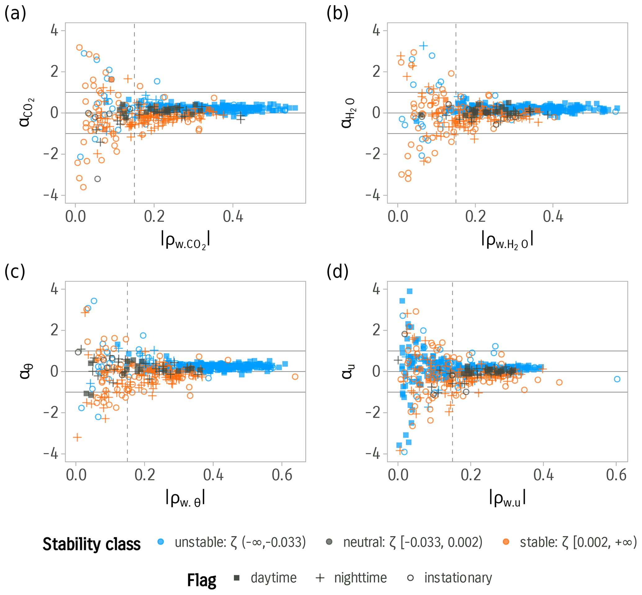
Figure 2Observed values of the transport asymmetry coefficient α vs. the correlation coefficient for four variables calculated from high-frequency measurements. (a) CO2, (b) H2O, (c) sonic temperature, θ, and (d) wind velocity component, u. Colors distinguish different stability classes. The point shape differentiates daytime, nighttime, and instationary conditions following Foken and Wichura (1996). The vertical dashed line is set to x=0.15, and the horizontal lines are set to and y=1.
The terms of Eq. (14) account for different contributions to the flux. The first term on the right-hand side is equivalent to calculating the flux as the difference in accumulated mass between updraft and downdraft. When , the equation is reduced to this term only. The second term accounts for the bias introduced by the biased advective term by using the weighted mean of the scalar and the magnitude of wind as an estimate for . We show that when , the first two terms are equivalent to using the concentration formula of Hicks and McMillen (1984) shown in Eq. (8), with the unequal volume correction of Turnipseed et al. (2009) that accounts for the small difference between the weighted mean and average of concentrations . Refer to Appendix A for details about this equality. The new third term corrects for the correlation between the scalar and the magnitude of the wind. Ignoring the third term will result in a flux biased with the ratio .
The new TEA equation reveals an important insight. When using the new equation to calculate the flux, the error in the flux when is independent of the scalar concentration and is governed by the characteristics of the turbulent transport. This strengthens confidence in using the TEA method for measuring atmospheric constituents with a high background concentration and small flux (low deposition velocity).
Using the new TEA formula with an estimated value for αc was effective in reducing the uncertainty and the systematic error in the calculated fluxes (Fig. 1). To quantify the magnitude of the systematic bias and uncertainty resulting from nonzero on the fluxes, we used the simulation results to obtain the slope and the coefficient of determination, R2, from a linear fit of the calculated fluxes against the reference EC flux. The simulation results show an increased bias and uncertainty in the fluxes when and a significant improvement when using an estimate of α for correction (Fig. 1).
We found that using the accumulated mass difference to calculate the TEA flux (first term in Eq. 14) produced the largest errors. Values of as small as 0.01 σw were sufficient to produce more than a 10 % mean bias in the flux magnitude for CO2 in our dataset.
The use of the concentration TEA equation of Hicks and McMillen (1984) was a considerable improvement over using the mass difference but still overestimated the TEA flux. The slope of the linear fit was 1.12 (R2=0.94). Using the DEA equation of Turnipseed et al. (2009), which includes an additional term to correct for the effect of unequal volume on the flux, led to underestimating the TEA flux, yielding a slope of 0.84 (R2=0.93). The correction of nonzero using αθ utilizing the assumption of scalar similarity significantly reduced the bias and the uncertainty and gave a slope of 1.005 (R2=0.995). The use of the analytical value of αc using Eq. (26) similarly reduced the bias but with a smaller reduction in uncertainty, yielding a slope of 0.991 (R2=0.97). The higher uncertainty when using the analytical value of αc is likely due to the deviation from the assumed Gaussian probability distribution.
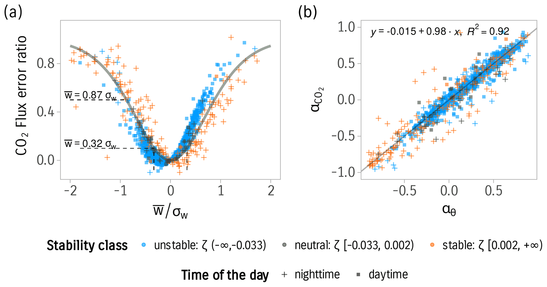
Figure 3(a) The error ratio in the CO2 flux calculated using the TEA method due to nonzero mean vertical wind. The solid gray line represents the analytical values of the error in the flux (if a joint Gaussian probability distribution is assumed). The points are the observed error calculated from high-frequency measurements colored according to stability classes. The point shape distinguishes daytime and nighttime data. (b) Relation of calculated for CO2 and αθ calculated from sonic temperature along with a 1-to-1 line for reference.
These results indicate that the proposed corrections using an estimate of αc are very effective in minimizing or removing the bias from TEA flux when even when using the analytical value of αc.
4.2 Value and interpretation of the transport asymmetry coefficient α
The value of αc defined in Eq. (12) indicates the disparity of the flux transport between updrafts and downdrafts. Values of αc larger than 1 indicate that updraft flux (S1+S4) and downdraft flux (S2+S3) have opposing signs. This pattern indicates that the wind and the scalar are correlated for updraft flux and anticorrelated for the downdraft flux (or the other way around). This pattern violates the stationarity conditions.
Therefore, we conclude that for stationary flows the systematic error in the TEA flux is smaller than . Observed values of α for H2O, CO2, θ, and the wind component, u, are shown in Fig. 2. The data confirm that values of are consistently below 1 for the four scalars when the stationarity criterion is met. However, when the correlation between w and the scalar is low during conditions associated with low developed turbulence, spurious correlations might lead to values of larger than 1.
We found that the value of α for CO2 moderately correlates with the skewness of the measured scalar (r=0.61, data not shown). The observed mean of α for CO2 and sonic temperature calculated from high-frequency measurements for periods with negligible was approximately 0.2 for unstable and good turbulent mixing conditions () with a standard error of SE=0.01. For stable stratification (ζ>0), the mean of α was approximately equal to −0.18 but with a higher spread around the mean: SE=0.09. These values indicate that updrafts have a larger contribution to the flux under unstable stratification and smaller contribution during stable stratification. The results generally agree with values found from studies using conditional sampling (Greenhut and Khalsa, 1982) and large eddy simulations (LESs) (Wyngaard and Moeng, 1992), which found that updraft contribution to the flux is 2 to 3 times larger than downdraft contribution under unstable conditions due to the contribution of convective thermals.
The sign of α indicates whether updrafts or downdrafts have a larger contribution to the flux. Inspecting Eq. (25), we find that a positive α indicates that the magnitude of updraft contribution to the flux is larger than the magnitude of the downdraft contribution (), while the opposite is true for a negative α.
The analytical value of α from Eq. (26) was effective in minimizing the systematic bias as confirmed by the simulation results. However, the assumption of a Gaussian distribution, although used in the literature, e.g., Wyngaard and Moeng (1992), is not adequate. While the wind might be normally distributed for most stability classes (Chu et al., 1996), the scalar can significantly depart from normality (Berg and Stull, 2004). Other distributions might be more suited for approximating the joint probability distribution (Frenkiel and Klebanoff, 1973). For example, Katsouvas et al. (2007), using experimental data, showed that a third-order Gram–Charlier distribution was necessary and sufficient in most cases for describing the quadrant time and flux contributions. It is worth considering this distribution to find a better analytical formula to calculate the expectation of α.
The hypothesis of scalar similarity was proposed as another source for estimating the values of α. The similarity was empirically confirmed by investigating the values of αθ and αc from high-frequency measurements (Fig. 3). A linear fit with a slope of 0.98 and R2 of 0.92 was obtained during steady-state and well-developed turbulence conditions. During such conditions, αθ can substitute αc to calculate the flux correction ratio. However, the correction becomes large and unreliable in periods when σw and ρcw are small, associated with small fluxes during nighttime and stable conditions. Additionally, temperature is considered a poor proxy during nearly neutral conditions due to its contribution to buoyancy (McBean, 1973; Hicks et al., 1980). We noticed that the variance in α values is higher under weakly developed turbulence and experimentally determined the threshold for the optimum use of αθ for the correction as . Below this threshold, values of αθ larger than 1 are observed, making the correction unreliable. This threshold can be seen as an indicator for the violation of assumptions of homogeneity and stationarity or other problematic conditions. Similar uses for the correlation coefficient are common in the literature, e.g., Foken and Wichura (1996).
Another use of the formulation using α is to find a threshold above which the TEA flux measurement becomes unreliable. For example, if we define the bias in the flux as not exceeding 10 % of the flux, we can experimentally find that the error in the flux due to nonzero becomes larger than 10 % when exceeds 0.21σw for periods with good turbulent mixing conditions (). This threshold is close to the analytical value of 0.323 σw obtained from the Gaussian joint probability distribution. To push this threshold further, αθ calculated from sonic temperature can be used during good turbulent mixing conditions (). Simulations indicate that the average relative confidence interval for the predicted value of αθ from is 0.17 % of the fit value. In summary for this example, to keep the error in the flux below 10 %, αθ can be safely used to correct for biased as long as . This limit is considered forgiving and easy to achieve with online coordinate rotation and further rather simple online treatments. The only time when this limit is expected to be reached is when σw is very small (e.g., during nighttime conditions) where other problems such as low turbulent mixing and violations of the assumptions of the EC and TEA methods are expected to occur. These periods largely overlap with periods considered to be of low quality and are usually excluded from the analysis (Foken et al., 2012b).
To summarize, we find that the error in the TEA flux is constrained to for , which was shown here to be true for stationary conditions, which are at the focus of turbulent flux measurements. If a correction is desired to minimize this error, two options were presented to estimate αc: first, an analytical solution, and second, an estimate employing scalar similarity. Finally, with the use of αc, the typically observed systematic flux bias due to nonzero mean vertical wind velocity could be effectively characterized and minimized.
In this paper, we revised the theory of the true eddy accumulation method and extended its applicability to measure turbulent fluxes under nonideal conditions in which the mean vertical wind velocity during the averaging interval is not zero. The new generalized equation allows estimating the scalar mean during the flux averaging interval and defining conditions in which the error in the flux is significant.
The new formulation allowed constraining the relative systematic error in the TEA flux to the ratio under stationarity conditions. This systematic error was reduced to be a function of the disparity of atmospheric transport instead of having it scale with the scalar background concentration. This development significantly reduces the systematic bias in TEA fluxes under nonideal conditions, allowing the TEA method to be used indifferently with various atmospheric constituents.
The coefficient αc, defined to quantify the atmospheric transport asymmetry, has proved to be very useful in estimating and removing the error in measured TEA fluxes. We showed two methods for estimating αc to reduce the flux systematic bias: (i) an estimate of αc based on the assumption of flux variance similarity and (ii) an analytical expression based on the assumption of a Gaussian joint probability distribution of the scalar concentration and vertical wind velocity. Both of these estimation methods were shown to be effective in minimizing the systematic error in the flux when compared to conventional TEA formulas.
In conclusion, the results presented in this paper showed that it is possible to achieve minimum bias in the TEA flux under most atmospheric conditions as well as identify those conditions which are less favorable. We believe that these results increase confidence in using the TEA method for different atmospheric constituents and under a variety of atmospheric conditions.
We show here how the TEA flux formula of Hicks and McMillen (1984), originally formulated under the assumption of , is equivalent to using as an estimate for in the second term on the right-hand side of Eq. (2).
We write the conditional expectation of as
where sign(w) is the sign of vertical wind velocity. P(w↑) and P(w↓) are the observed probabilities of the sign of w, which equals the ratio of the time the wind is positive or negative to the total integration interval time:
and similarly
By substituting with
we obtain
After rearrangement and simplification we get to
When Eq. (A6) is compared with Eq. (2), it is clear that the term is used as an estimate for .
| Symbols | ||
| c | mol m−3 | Molar density of a scalar |
| w | m s−1 | Vertical wind velocity |
| Δt | s | Flux averaging interval |
| A | – | TEA sampling scaling factor |
| V | m3 | Volume |
| C | mol m−3 | Mean concentration of |
| accumulated samples | ||
| αc | – | Transport asymmetry coefficient |
| for scalar c | ||
| ρ | – | Correlation coefficient |
| Si | – | Flux contribution from quadrant i |
| Subscripts | ||
| acc | Accumulated samples | |
| ↑ | Updraft buffer volume | |
| ↓ | Downdraft buffer volume | |
| c | Atmospheric constituent |
Data and scripts needed for producing the results and the figures presented in this paper are provided in Emad and Siebicke (2022).
AE developed the generalized TEA equation, implemented needed software, analyzed the data, and wrote the paper. LS provided supervision and feedback on the results, analysis, and paper.
The contact author has declared that none of the authors has any competing interests.
Publisher's note: Copernicus Publications remains neutral with regard to jurisdictional claims in published maps and institutional affiliations.
We would like to thank the two referees (Christoph Thomas and an anonymous reviewer) and the editor for their constructive, useful, and detailed comments, which have significantly improved the paper. We gratefully acknowledge the support of the Bioclimatology group, led by Alexander Knohl at the University of Göttingen, in particular technical assistance by Justus Presse, Frank Tiedemann, Marek Peksa, Dietmar Fellert, and Edgar Tunsch. We thank Christian Brümmer, Jean-Pierre Delorme from the Thünen Institute for Agricultural Climate Protection, and Mathias Herbst from the Center for Agrometeorological Research of the German Meteorological Service (DWD) for facilitating the fieldwork in Braunschweig. We further acknowledge Christian Markwitz for the fruitful discussions during the preparation of the paper and for reading and commenting on the paper. We thank Alexander Knohl, Nicolò Camarretta, Justus van Ramshorst, and Yannik Wardius for reading the paper and providing useful comments.
This research has been supported by the Niedersächsische Ministerium für Wissenschaft und Kultur (Wissenschaft.Niedersachsen.Weltoffen grant), the H2020 European Research Council (grant no. 682512), and the Deutsche Forschungsgemeinschaft (grant no. INST 186/1118-1 FUGG).
This open-access publication was funded by the University of Göttingen.
This paper was edited by Hartwig Harder and reviewed by Christoph Thomas and one anonymous referee.
Baldocchi, D.: Measuring Fluxes of Trace Gases and Energy between Ecosystems and the Atmosphere – the State and Future of the Eddy Covariance Method, Global Change Biol., 20, 3600–3609, https://doi.org/10.1111/gcb.12649, 2014. a
Baldocchi, D. D., Hicks, B. B., and Meyers, T. P.: Measuring Biosphere-Atmosphere Exchanges of Biologically Related Gases with Micrometeorological Methods, Ecology, 69, 1331–1340, https://doi.org/10.2307/1941631, 1988. a
Berg, L. K. and Stull, R. B.: Parameterization of Joint Frequency Distributions of Potential Temperature and Water Vapor Mixing Ratio in the Daytime Convective Boundary Layer, J. Atmos. Sci., 61, 813–828, https://doi.org/10.1175/1520-0469(2004)061<0813:POJFDO>2.0.CO;2, 2004. a
Bowling, D. R., Turnipseed, A. A., Delany, A. C., Baldocchi, D. D., Greenberg, J. P., and Monson, R. K.: The Use of Relaxed Eddy Accumulation to Measure Biosphere-Atmosphere Exchange of Isoprene and Other Biological Trace Gases, Oecologia, 116, 306–315, https://doi.org/10.1007/s004420050592, 1998. a
Businger, J. A. and Oncley, S. P.: Flux Measurement with Conditional Sampling, J. Atmos. Ocean. Technol., 7, 349–352, https://doi.org/10.1175/1520-0426(1990)007<0349:FMWCS>2.0.CO;2, 1990. a, b, c, d
Chu, C. R., Parlange, M. B., Katul, G. G., and Albertson, J. D.: Probability Density Functions of Turbulent Velocity and Temperature in the Atmospheric Surface Layer, Water Resour. Res., 32, 1681–1688, https://doi.org/10.1029/96WR00287, 1996. a
Desjardins, R. L.: Energy Budget by an Eddy Correlation Method, J. Appl. Meteorol., 16, 248–250, https://doi.org/10.1175/1520-0450(1977)016<0248:EBBAEC>2.0.CO;2, 1977. a, b
Emad, A. and Siebicke, L.: Reproduction Data and Code for the Paper: True Eddy Accumulation – Part 1: Solutions to the Problem of Non-Vanishing Mean Vertical Wind Velocity, Zenodo [data set, code], https://doi.org/10.5281/zenodo.7047610, 2022. a
Emad, A. and Siebicke, L.: True eddy accumulation – Part 2: Theory and experiment of the short-time eddy accumulation method, Atmos. Meas. Tech., 16, 41–55, https://doi.org/10.5194/amt-16-41-2023, 2023. a
Finnigan, J. J., Clement, R., Malhi, Y., Leuning, R., and Cleugh, H.: A Re-Evaluation of Long-Term Flux Measurement Techniques Part I: Averaging and Coordinate Rotation, Bound. Lay. Meteorol., 107, 1–48, https://doi.org/10.1023/A:1021554900225, 2003. a
Foken, T. and Wichura, B.: Tools for Quality Assessment of Surface-Based Flux Measurements, Agr. Forest Meteorol., 78, 83–105, https://doi.org/10.1016/0168-1923(95)02248-1, 1996. a, b
Foken, T., Gockede, M., Mauder, M., Mahrt, L., Amiro, B., and Munger, W.: Post-Field Data Quality Control, Handbook of Micrometeorology, 29, 181–208, https://doi.org/10.1007/1-4020-2265-4_9, 2004. a
Foken, T., Göockede, M., Mauder, M., Mahrt, L., Amiro, B., and Munger, W.: Post-Field Data Quality Control, in: Handbook of Micrometeorology: A Guide for Surface Flux Measurement and Analysis, edited by: Lee, X., Massman, W., and Law, B., Atmospheric and Oceanographic Sciences Library, 181–208, Springer Netherlands, Dordrecht, https://doi.org/10.1007/1-4020-2265-4_9, 2005. a
Foken, T., Aubinet, M., and Leuning, R.: The Eddy Covariance Method, in: Eddy Covariance: A Practical Guide to Measurement and Data Analysis, edited by: Aubinet, M., Vesala, T., and Papale, D., Springer Atmospheric Sciences, 1–19, Springer Netherlands, Dordrecht, https://doi.org/10.1007/978-94-007-2351-1_1, 2012a. a
Foken, T., Leuning, R., Oncley, S. R., Mauder, M., and Aubinet, M.: Corrections and Data Quality Control, in: Eddy Covariance: A Practical Guide to Measurement and Data Analysis, edited by: Aubinet, M., Vesala, T., and Papale, D., Springer Atmospheric Sciences, 85–131, Springer Netherlands, Dordrecht, https://doi.org/10.1007/978-94-007-2351-1_4, 2012b. a
Frenkiel, F. N. and Klebanoff, P. S.: Probability Distributions and Correlations in a Turbulent Boundary Layer, The Phys. Fluids, 16, 725–737, https://doi.org/10.1063/1.1694421, 1973. a
Fuehrer, P. L. and Friehe, C. A.: Flux Corrections Revisited, Bound. Lay. Meteorol., 102, 415–458, https://doi.org/10.1023/A:1013826900579, 2002. a
Greenhut, G. K. and Khalsa, S. J. S.: Updraft and Downdraft Events in the Atmospheric Boundary Layer Over the Equatorial Pacific Ocean, J. Atmos. Sci., 39, 1803–1818, https://doi.org/10.1175/1520-0469(1982)039<1803:UADEIT>2.0.CO;2, 1982. a
Gu, L., Massman, W. J., Leuning, R., Pallardy, S. G., Meyers, T., Hanson, P. J., Riggs, J. S., Hosman, K. P., and Yang, B.: The Fundamental Equation of Eddy Covariance and Its Application in Flux Measurements, Agr. Forest Meteorol., 152, 135–148, https://doi.org/10.1016/j.agrformet.2011.09.014, 2012. a, b
Heinesch, B., Yernaux, M., and Aubinet, M.: Some Methodological Questions Concerning Advection Measurements: A Case Study, Bound. Lay. Meteorol., 122, 457–478, https://doi.org/10.1007/s10546-006-9102-4, 2007. a
Hicks, B. B. and Baldocchi, D. D.: Measurement of Fluxes Over Land: Capabilities, Origins, and Remaining Challenges, Bound. Lay. Meteorol., 177, 365–394, https://doi.org/10.1007/s10546-020-00531-y, 2020. a
Hicks, B. B. and McMillen, R. T.: A Simulation of the Eddy Accumulation Method for Measuring Pollutant Fluxes, J. Climate Appl. Meteorol., 23, 637–643, https://doi.org/10.1175/1520-0450(1984)023<0637:ASOTEA>2.0.CO;2, 1984. a, b, c, d, e, f, g, h
Hicks, B. B., Wesely, M. L., and Durham, J. L.: Critique of Methods to Measure Dry Deposition Workshop Summary, Tech. Rep. PB-81126443; EPA-600/9-80-050, Argonne National Lab., IL (USA), Environmental Protection Agency, Research Triangle Park, NC (USA), 1980. a
Katsouvas, G. D., Helmis, C. G., and Wang, Q.: Quadrant Analysis of the Scalar and Momentum Fluxes in the Stable Marine Atmospheric Surface Layer, Bound. Lay. Meteorol., 124, 335–360, https://doi.org/10.1007/s10546-007-9169-6, 2007. a, b
Katul, G., Kuhn, G., Schieldge, J., and Hsieh, C.-I.: The Ejection-Sweep Character of Scalar Fluxes in the Unstable Surface Layer, Bound. Lay. Meteorol., 83, 1–26, https://doi.org/10.1023/A:1000293516830, 1997. a
Lee, X., Finnigan, J., and Paw U, K. T.: Coordinate Systems and Flux Bias Error, in: Handbook of Micrometeorology: A Guide for Surface Flux Measurement and Analysis, edited by: Lee, X., Massman, W., and Law, B., Atmospheric and Oceanographic Sciences Library, 33–66, Springer Netherlands, Dordrecht, https://doi.org/10.1007/1-4020-2265-4_3, 2005. a
Lenschow, D. H., Mann, J., and Kristensen, L.: How Long Is Long Enough When Measuring Fluxes and Other Turbulence Statistics?, J. Atmos. Ocean. Technol., 11, 661–673, https://doi.org/10.1175/1520-0426(1994)011<0661:HLILEW>2.0.CO;2, 1994. a
Leone, F. C., Nelson, L. S., and Nottingham, R. B.: The Folded Normal Distribution, Technometrics, 3, 543–550, https://doi.org/10.1080/00401706.1961.10489974, 1961. a
McBean, G. A.: Comparison of the Turbulent Transfer Processes near the Surface, Bound. Lay. Meteorol., 4, 265–274, https://doi.org/10.1007/BF02265237, 1973. a
Monin, A. S. and Obukhov, A. M.: Basic Laws of Turbulent Mixing in the Ground Layer of the Atmosphere, Translated for Geophysics Research Directorate, AF Cambridge Research Center... by the American meteorological Society, Tr. Akad. Nauk SSSR Geophiz. Inst., Boston, MA, 24, 163–187, 1954. a
Ohtaki, E.: On the Similarity in Atmospheric Fluctuations of Carbon Dioxide, Water Vapor and Temperature over Vegetated Fields, Bound. Lay. Meteorol., 32, 25–37, https://doi.org/10.1007/BF00120712, 1985. a
Pattey, E., Desjardins, R. L., and Rochette, P.: Accuracy of the Relaxed Eddy-Accumulation Technique, Evaluated Using CO2 Flux Measurements, Bound. Lay. Meteorol., 66, 341–355, https://doi.org/10.1007/BF00712728, 1993. a, b
Paw U, K. T., Baldocchi, D. D., Meyers, T. P., and Wilson, K. B.: Correction Of Eddy-Covariance Measurements Incorporating Both Advective Effects And Density Fluxes, Bound. Lay. Meteorol., 97, 487–511, https://doi.org/10.1023/A:1002786702909, 2000. a
Rannik, Ü., Vesala, T., Peltola, O., Novick, K. A., Aurela, M., Järvi, L., Montagnani, L., Mölder, M., Peichl, M., Pilegaard, K., and Mammarella, I.: Impact of Coordinate Rotation on Eddy Covariance Fluxes at Complex Sites, Agr. Forest Meteorol., 287, 107940, https://doi.org/10.1016/j.agrformet.2020.107940, 2020. a, b
Raupach, M. R.: Conditional Statistics of Reynolds Stress in Rough-Wall and Smooth-Wall Turbulent Boundary Layers, J. Fluid Mechan., 108, 363–382, https://doi.org/10.1017/S0022112081002164, 1981. a
Rinne, J. and Ammann, C.: Disjunct Eddy Covariance Method, in: Eddy Covariance: A Practical Guide to Measurement and Data Analysis, edited by: Aubinet, M., Vesala, T., and Papale, D., Springer Atmospheric Sciences, 291–307, Springer Netherlands, Dordrecht, https://doi.org/10.1007/978-94-007-2351-1_10, 2012. a
Rinne, H. J. I., Delany, A. C., Greenberg, J. P., and Guenther, A. B.: A True Eddy Accumulation System for Trace Gas Fluxes Using Disjunct Eddy Sampling Method, J. Geophys. Res.-Atmos., 105, 24791–24798, https://doi.org/10.1029/2000JD900315, 2000. a
Rinne, J., Tuovinen, J.-P., Laurila, T., Hakola, H., Aurela, M., and Hypén, H.: Measurements of Hydrocarbon Fluxes by a Gradient Method above a Northern Boreal Forest, Agr. Forest Meteorol., 102, 25–37, https://doi.org/10.1016/S0168-1923(00)00088-5, 2000. a
Siebicke, L. and Emad, A.: True eddy accumulation trace gas flux measurements: proof of concept, Atmos. Meas. Tech., 12, 4393–4420, https://doi.org/10.5194/amt-12-4393-2019, 2019. a
Sun, J.: Tilt Corrections over Complex Terrain and Their Implication for CO2 Transport, Bound. Lay. Meteorol., 124, 143–159, https://doi.org/10.1007/s10546-007-9186-5, 2007. a
Thomas, C. and Foken, T.: Flux Contribution of Coherent Structures and Its Implications for the Exchange of Energy and Matter in a Tall Spruce Canopy, Bound. Lay. Meteorol., 123, 317–337, https://doi.org/10.1007/s10546-006-9144-7, 2007. a
Turnipseed, A. A., Pressley, S. N., Karl, T., Lamb, B., Nemitz, E., Allwine, E., Cooper, W. A., Shertz, S., and Guenther, A. B.: The use of disjunct eddy sampling methods for the determination of ecosystem level fluxes of trace gases, Atmos. Chem. Phys., 9, 981–994, https://doi.org/10.5194/acp-9-981-2009, 2009. a, b, c, d, e, f
Webb, E. K., Pearman, G. I., and Leuning, R.: Correction of Flux Measurements for Density Effects Due to Heat and Water Vapour Transfer, Q. J. Roy. Meteorol. Soc., 106, 85–100, https://doi.org/10.1002/qj.49710644707, 1980. a
Wesely, M. L.: Use of Variance Techniques to Measure Dry Air-Surface Exchange Rates, Bound. Lay. Meteorol., 44, 13–31, https://doi.org/10.1007/BF00117291, 1988. a
Wilczak, J. M., Oncley, S. P., and Stage, S. A.: Sonic Anemometer Tilt Correction Algorithms, Bound. Lay. Meteorol., 99, 127–150, https://doi.org/10.1023/A:1018966204465, 2001. a
Wyngaard, J. C. and Moeng, C.-H.: Parameterizing Turbulent Diffusion through the Joint Probability Density, Bound. Lay. Meteorol., 60, 1–13, https://doi.org/10.1007/BF00122059, 1992. a, b
- Abstract
- Introduction
- Theory
- Methods
- Results and discussion
- Conclusions
- Appendix A: Hicks and McMillen formulation
- Appendix B: Symbols and subscripts with units
- Code and data availability
- Author contributions
- Competing interests
- Disclaimer
- Acknowledgements
- Financial support
- Review statement
- References