Field evaluation of low-cost electrochemical air quality gas sensors under extreme temperature and relative humidity conditions

Modern electrochemical gas sensors hold great potential for improving practices in air quality (AQ) monitoring as their low cost, ease of operation and compact design can enable dense observational networks and mobile measurements. Despite that, however, numerous studies have shown that the performance of these sensors depends on a number of factors (e.g. environmental conditions, sensor quality, maintenance and calibration), thereby adding significant uncertainties in the reported measurements and large discrepancies from those recorded by reference-grade instruments. In this work we investigate the performance of electrochemical sensors, provided by two manufacturers (namely Alphasense and Winsen), for measuring the concentrations of CO, NO₂, O₃ and SO₂. To achieve that we carried out collocated yearlong measurements with reference-grade instruments at a traffic AQ monitoring station in Nicosia, Cyprus, where temperatures ranged from ca. 0 ^∘C in the winter to almost 45 ^∘C in the summer. The CO sensors exhibit the best performance among all the ones we tested, having minimal mean relative error (MRE) compared to reference instruments (ca. −5 %), although a significant difference in their response was observed before and after the summer period. At the other end of the spectrum, the SO₂ sensors reported concentration values that were at least 1 order of magnitude higher than the respective reference measurements (with MREs being more than 1000 % for Alphasense and almost 400 % for Winsen throughout the entire measurement period), which can be justified by the fact that the concentrations of SO₂ at our measuring site were below their limit of detection. In general, variabilities in the environmental conditions (i.e. temperature and relative humidity) appear to significantly affect the performance of the sensors. When compared with reference instruments, the CO and NO₂ electrochemical sensors provide measurements that exhibit increasing errors and decreasing correlations as temperature increases (from below 10 to above 30 ^∘C) and RH decreases (from >75 % to below 30 %). Interestingly, the performance of the sensors was affected irreversibly during the hot summer period, exhibiting different responses before and after that, resulting in a signal deterioration that was more than twice that reported by the manufacturers. With the exception of the Alphasense NO₂ sensor, all low-cost sensors (LCSs) exhibited measurement uncertainties that were much higher, even at the beginning of our measurement period, compared to those required for qualifying the sensors for indicative air quality measurements according to the respective European Commission (EC) Directive. Overall, our results show that the response of all LCSs is strongly affected by the environmental conditions, warranting further investigations on how they are manufactured, calibrated and employed in the field.

1 Introduction

Air pollution accounts for more than 7 million premature deaths around the globe on an annual basis (Lelieveld et al., 2020), making it the fourth-greatest overall risk factor for human health (Juginovic et al., 2021). Recognising this risk, the concentration of key pollutants has to be continuously monitored, especially in the urban environment, in order to ensure that they do not exceed certain limit values. Although wide networks of air quality (AQ) monitoring stations have been established in many cities around the globe for this reason, the spatial distribution of the observations is still limited for providing detailed AQ mapping over urban agglomerates. This, in turn, limits our ability to effectively associate urban air pollution with potential human health effects and to design effective mitigation strategies.

Building AQ monitoring networks that go far beyond the current state-of-the-art with respect to their spatial coverage is limited by the required high capital, operational and maintenance costs. The city of Paris, for instance, operates 13 measuring sites (AIRPARIF, 2018), whereas in London, AQ is monitored at around 100 locations (Greater London Authority, 2018). Although these numbers are seemingly high, they correspond to a spatial coverage of the order of one station over a few tens of square kilometres. This limitation can be lifted by employing low-cost sensors (LCSs) in dense observational networks that can enable quick and effective identification of pollution sources and determination of concentration gradients over specific areas.

According to the World Meteorological Organization (WMO), LCSs are defined as systems that are at least 1 order of magnitude less expensive compared to reference instruments (WMO, 2018). Electrochemical (ECh) sensors, which fall into this category, have received great attention in recent years as their low cost, compact size and response time (on the order of a minute) can enable their use in dense AQ monitoring networks and easy-to-carry-out mobile measurements. The low price of these sensors, however, comes at a cost in performance and in the quality of the data they provide compared to reference-grade instruments, which can be attributed to a number of factors, including cross-sensitivities (Lewis et al., 2015; Mead et al., 2013), signal drifts over time and low life expectancies (Mead et al., 2013; Smith et al., 2017; Popoola et al., 2016; Hagan et al., 2018), low sensitivities (Borrego et al., 2016), and variabilities related to environmental conditions (Castell et al., 2017; Jerrett et al., 2017; Spinelle et al., 2015, 2017; Cross et al., 2017; Pang et al., 2017; Aleixandre and Gerboles, 2012; Masson et al., 2015).

An increasing number of studies have investigated the performance of LCSs under different conditions (Hagan et al., 2018; Mead et al., 2013; Jerrett et al., 2017; Cross et al., 2017; Jiao et al., 2016; Bílek et al., 2021; Collier-Oxandale et al., 2020; Liang et al., 2021). Closer comparison of the results from some of the abovementioned studies, in which the performance of the same sensors (i.e. Alphasense B series) was tested, but at different locations and under different conditions, shows that the variability in the environmental conditions plays a significant role, provided the concentrations of the target gases are above their limit of detection (LoD) (Borrego et al., 2016; Castell et al., 2017; Cross et al., 2017; Bauerová et al., 2020; Karagulian et al., 2019). In a study carried out in Norway, during which the temperature and relative humidity (RH) varied from −0.7 to 23.3 ^∘C and from 19 % to 98 %, respectively, the mean bias error (MBE) of the measurements reported by the CO and NO₂ LCSs when compared with reference measurements were −147.2 and 13.3 ppb, respectively, whereas the associated correlations (R²) were 0.36 for the CO and 0.24 for the NO₂ LCS (Castell et al., 2017). In a similar study carried out in Portugal, where the temperature varied from 15 to 30 ^∘C and the RH from 39 % to 87 %, the overall performance of the same sensors was better, exhibiting lower averaged MBEs (−0.025 ppb for CO and 7.1 ppb for NO₂) and higher R² (0.76 for CO and 0.58 for NO₂; Borrego et al., 2016).

Operating temperature and RH are two of the most important factors affecting the performance of ECh sensors, mainly because they employ aqueous electrolytes containing sulfuric acid for the transfer of charges between the measuring and the reference electrodes. The concentration of sulfuric acid in the electrolyte is 5 M, which requires 60 % RH at 20 ^∘C in ambient air to be in equilibrium (Alphasense, 2013). Exposure of the sensors to RH levels less than 60 % can in principle lead to evaporation of the solvent (i.e. water), whereas the opposite can happen under RH conditions above 60 %. According to the manufacturer, the Alphasense ECh sensors can provide meaningful measurements even when exposed to RH values down to 15 % or up to 90 % at ambient temperature as long as they have enough time to equilibrate to the new conditions, i.e. several days. Ideally, when ECh sensors are exposed over long periods to RH values far from 60 %, they need to be recalibrated under the new RH conditions. However, considering that ambient RH is highly variable and that it can change significantly within a few hours, using RH-dependent calibration turns out to be impractical.

It should be noted that field tests of LCSs reported in the literature were conducted at different locations, in different seasons and over durations that range from 2 weeks (Borrego et al., 2016) to 4.5 months (Cross et al., 2017). This makes any direct comparison and further analysis of the data for understanding how the environmental conditions affect the performance of the LCSs highly challenging (Karagulian et al., 2019). In addition to the potential effects of the environmental conditions on the accuracy of LCSs, the long-term performance of LCSs can systematically vary over time as they can exhibit significant signal drifts (WMO, 2018; Jiao et al., 2016; Masson et al., 2015). To address these issues, we urgently need systematic observations at different locations and under different conditions over long periods of time.

In this work we compare yearlong measurements of the concentration of key gaseous pollutants (i.e. CO, NO₂, O₃ and SO₂) reported by low-cost ECh sensors, manufactured by Alphasense and Winsen, and by reference-grade instruments. The measurements took place at a traffic station in the city of Nicosia, Cyprus, where the LCSs were exposed to highly variable gaseous concentrations (which were affected by both local and regional pollution sources) and variable environmental conditions. The site is characterised by a high number of sunny days and long hot summers, when the temperature and RH can reach values up to ca. 50 ^∘C and below 10 %, respectively, providing a unique setting for testing the performance of these sensors under extreme conditions.

2 Methods

2.1 Low-cost gas sensors

ECh sensors manufactured by Alphasense and Winsen were tested in this study. More specifically, we employed the analogue Alphasense B series gas sensors (Models CO-B41, NO₂-B43F, OX-B431 and SO₂-B4) and the digital Winsen ZE12 model sensors configured by the manufacturer to measure the concentration of CO, NO₂, O₃ and SO₂.

The operating principle of ECh sensors relies on redox reactions that take place on the surface of their sensing electrode, which is also referred to as the working electrode (WE). More specifically, the gas molecules reaching the surface of the WE get either oxidised or reduced, consequently providing or capturing electrons to/from the system depending on their electronegativity. An ECh cell is completed by the so-called counter electrode (CE) that balances the charge variabilities from the reactions at the surface of the WE. This charge balancing happens by transferring electrons through an electrolyte serving as the medium for transporting the charge carriers from one electrode to the other. The electrical signal (i.e. current) produced by this process is proportional to the concentration of the reducing/oxidising gas interacting with the WE. In some ECh sensors, a reference electrode (RE) is used to maintain the potential of the WE at a fixed value.

All ECh LCSs employed in this work use the abovementioned three-electrode configuration. The Alphasense sensors employ an additional electrode, namely the auxiliary electrode (AE), which has similar characteristics to those of the WE but is incorporated in the cell in such a way that it is not exposed to the target gas. A background current, caused by all other factors except the interaction of the WE with the target gas, is induced on the AE. It should be noted that the WE measures the combined current, which is the sum of the background current and the current induced by the target gas when reacting with it. The AE current is then subtracted from the WE current, giving the compensated WE current (i.e. without the background signal) that corresponds solely to the interaction of the sensing electrode with the target gas (Alphasense, 2019).

The specifications of all the LCSs we employed are provided in Tables S1 and S2 in the Supplement. For our tests the sensors were placed in two waterproof boxes – one containing the Alphasense and the other the Winsen LCSs (see Fig. 1a and b, respectively) – with the sensing side facing outside, as shown in Fig. 1c. The boxes, referred to as the AQ monitors from this point onwards, were protected with a reflective cover to avoid direct exposure to sunlight and attached on a railing within 1 m distance from the inlet of the reference instruments (see Fig. 1d). Both monitors were installed at the rooftop of the reference AQ monitoring station (see description further below) from October 2019 to December 2020 and operated continuously, with some interruptions during the high-temperature season.

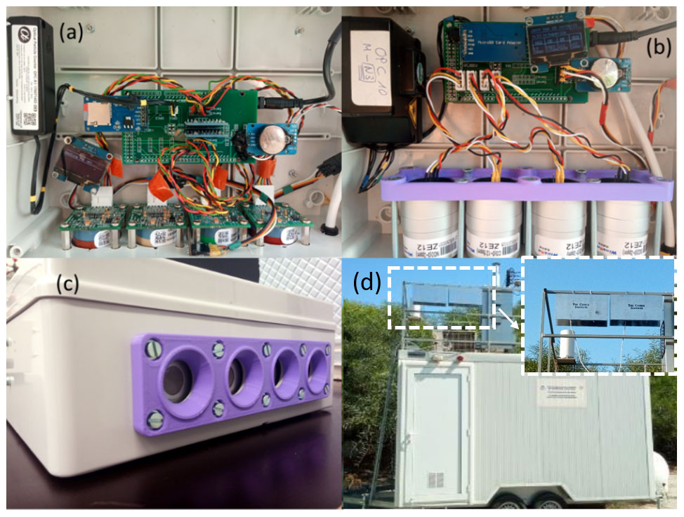
Figure 1 Images showing the layout of the AQ monitors housing the Alphasense (a) and the Winsen (b) LCSs, the side of the AQ monitors at which the sensing elements of the LCSs were exposed to the ambient air (c), and the place that the AQ monitors were installed at the top of the reference station (d).

To run the AQ monitors and record the data from the LCSs we built an electronic circuit board (see Fig. 1a and b) comprised of a microcontroller (Atmel, Model AVR Mega 2560), a real-time clock (RTC; Maxim, Model DS3231), a display and a Secure Digital (SD) card. For the Alphasense gas sensors that have a dual analogue output, an analogue-to-digital converter (ADC; Texas Instruments, Model ADS1115) was employed to convert their analogue voltage signals to digital values. The Winsen LCSs have a digital output in the Universal Asynchronous Receiver–Transmitter (UART) protocol, so no conversion was needed. The data from the LCSs were stored on the SD cards every 2 s for the Alphasense sensors and every 5 s for the Winsen sensors. The RTC, ADC and display communicated with the microcontroller via an inter-integrated circuit (I2C), whereas the SD card was accessed via the Serial Peripheral Interface (SPI) protocol. Figure S1 in the Supplement shows the schematic of the electronic circuit employed in the AQ monitors.

2.2 Measurement site

The site used for our measurements is a traffic AQ monitoring station in Nicosia, Cyprus, with latitude and longitude coordinates of 35^∘9^′7.20^′′ N, 33^∘20^′52.03^′′ E. The station is located at a distance of 10 m from one of the main and busiest city avenues (see Fig. 2), which is typically congested during the morning and the afternoon rush hours. The site is considered a reference AQ station as the measurements follow the relevant European Commission (EC) Directives and the corresponding national laws defining the specifications that the employed instruments must meet, as well as the measurement procedures that must be followed, which are also in accordance with international quality standards (EC, 2008). The reference instruments used at the station together with their characteristics are listed in Table S2.

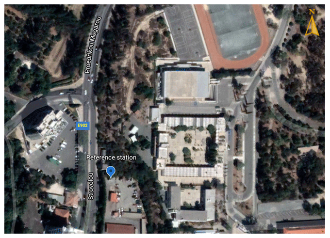
Figure 2 Satellite image showing the location of the traffic AQ monitoring station in Nicosia, where the measurements reported in this study were carried out. The station is located ca. 10 m from Strovolou Avenue, which is a rather busy road, especially during the morning and afternoon rush hours. Map data are from © Google, DigitalGlobe.

We should highlight here that Cyprus is an island in the eastern Mediterranean, a region that is a crossroad of polluted air masses coming from three continents (namely Europe, Asia and Africa; Lelieveld et al., 2002). Local sources contribute to the background AQ of the region, creating a highly interesting blend of air pollutants. In addition, the region is characterised by a high number of sunny days with intense ultraviolet (UV) radiation, resulting in a strong atmospheric photochemical activity compared to other European countries (Vrekoussis et al., 2022). According to the national authority for regulatory monitoring, the main sources of CO observed on the island are related to local fossil fuel burning (i.e. energy production, transportation and central heating), with typical annual concentrations of more than 250 µg m⁻³ (153 ppb; DLI Annual Technical Report Air Quality, 2020). The primary sources of NO₂ and SO₂ emissions are also from fossil fuel burning, with typical mean annual concentrations of more than 15 µg m⁻³ (ca. 9 ppb) and 2 µg m⁻³ (ca. 1 ppb), respectively (DLI Annual Technical Report Air Quality, 2020), whereas the annual mean concentration of O₃ is ca. 70 µg m⁻³ (ca. 35 ppb).

2.3 Calibration of the LCSs

The Alphasense gas sensors employed in this work were accompanied by an individual sensor board (ISB), which converts the signal from the WE and AE to voltages and facilitates data acquisition using ADCs. The electronic and zero offsets of the WE and AE signals, as well as the sensitivity and temperature correction factors, were also provided by the manufacturer for each sensor following laboratory calibration. These values were used to convert the measured signals to concentrations of pollutants by first calculating the corrected WE voltage value and then dividing by the sensor sensitivity. The manufacturer provides four different equations for the conversion of the raw signals from the WE and the AE to gas concentrations (ppb) for each sensor. The equations used in this work were the ones converting the raw signals (Papaconstantinou et al., 2023) to concentrations that are in better agreement with those reported by the reference instruments. For the CO and O₃ sensors this is

$$\begin{array}{}\text{(1)}& C={\displaystyle \frac{V_{\mathrm{WEc}}}{S}}={\displaystyle \frac{\left(V_{\mathrm{WEu}}-V_{\mathrm{WEe}}\right)-n_T\times \left(V_{\mathrm{AEu}}-V_{\mathrm{AEe}}\right)}{S}},\end{array}$$

where V_WEu is the uncorrected raw WE output, V_WEe is the WE electronic offset on the ISB, n_T is a temperature-dependent correction factor, V_AEu is the uncorrected raw AE output, V_AEe is the AE electronic offset on the ISB, and S is the sensitivity. We should note here that all the electrode signals are provided in millivolts, whereas the sensitivity of the sensors is expressed in millivolts per part per billion. To account for cross-sensitivity of the O₃ LCS from NO₂, the first term in the nominator of Eq. (1) becomes $V_{\mathrm{WEu}}-V_{\mathrm{WEe}}-V_{\mathrm{WEc}\left(\mathrm{NO}\mathrm{2}\right)}$, where V_WEc(NO2) is the voltage induced on the working electrode, calculated using the NO₂ concentration measured from the NO₂ LCS, multiplied by the sensitivity (mV per ppb) of the O₃ sensor to NO₂, following the guidelines of the manufacturer (Alphasense, 2019). For the NO₂ and the SO₂ sensors, the equation yielding concentration values that compared better with those of the reference instrument is

$$\begin{array}{}\text{(2)}& \begin{array}{rl}C& ={\displaystyle \frac{V_{\mathrm{WEc}}}{S}}\\ & ={\displaystyle \frac{\left(V_{\mathrm{WEu}}-V_{\mathrm{WEe}}\right)-k_T\times \left(\frac{V_{{\mathrm{WE}}_{\mathrm{0}}}}{V_{{\mathrm{AE}}_{\mathrm{0}}}}\right)\left(V_{\mathrm{AEu}}-V_{\mathrm{AEe}}\right)}{S}}.\end{array}\end{array}$$

Here $V_{{\mathrm{WE}}_{\mathrm{0}}}$ is the WE output in zero air (i.e. air without the target gas), $V_{{\mathrm{AE}}_{\mathrm{0}}}$ is the AE output in zero air, and k_T is the temperature-dependent correction factor.

Temperature is used as input for the calculation of the correction factors n_T and k_T in Eqs. (1) and (2). The values of n_T and k_T are provided by the manufacturer for specific temperatures, ranging from ca. −30 to 50 ^∘C with 10 ^∘C intervals, are shown in the Supplement (Table S3). It should be noted that for a more accurate calculation of the temperature correction factors in our analysis, we used linear (for CO) or spline (for NO₂, O₃ and SO₂) interpolations, as shown in Fig. S2. While a temperature/RH sensor was included inside the two AQ monitors, the temperatures used as input for the calculation of the correction factors n_T and k_T are the ones measured by the reference thermometers at the station. We should note here that the temperature and RH sensor used in the two AQ monitors recorded measurements that deviated substantially from those reported by the reference sensors and thus were not used for determining the concentrations from the LCSs.

The Winsen ZE12 gas sensors are general-purpose sensors that can measure the concentration of CO, SO₂, NO₂ and O₃ based on the ECh sensor principle. In contrast to their Alphasense counterparts, these sensors do not come with a specific calibration equation to account for temperature variabilities. Instead, measurements from a built-in temperature sensor are used internally to capture respective variabilities, providing signal outputs that are directly expressed as concentrations (ppb). It should be noted that an offset of ca. 400 ppb in the raw measurements from the Winsen CO LCS was observed throughout the entire period of our study and that this value has been subtracted from the reported data to facilitate comparison with the measurements by the respective reference instrument.

2.4 Data analysis

As stated above, the WE and AE outputs from the Alphasense LCSs were recorded every 2 s, whereas the concentrations from the Winsen LCSs were recorded every 5 s. All LCS measurements were averaged over a period of an hour for direct comparison with the observations provided by the reference instruments. After converting raw signals to concentrations, negative values were omitted. The effect of the environmental parameters (i.e. temperature and RH) on the performance of the sensors was assessed by dividing the whole dataset into different temperature (i.e. <10, 10–20, 20–30 and >30 ^∘C) and RH (i.e. <30 %, 30 %–55 %, 55 %–75 % and >75 %) ranges. These ranges were selected considering the minimum and maximum temperature and RH values encountered during our measurement period and the conditions under which the LCSs are calibrated in the laboratory by the manufacturer (i.e. T=20 ^∘C and RH = 60 %).

The performance of the LCSs is evaluated by directly correlating and comparing the reported concentrations with measurements by the respective reference instruments to determine the associated errors. The parameters used to do so were the coefficient of determination (R²), the mean bias error (MBE), the mean relative error (MRE), the mean absolute error (MAE) and the normalised root mean square error (NRMSE), defined respectively as follows:

$$\begin{array}{}\text{(3)}& {\displaystyle }{R}^{\mathrm{2}}=\mathrm{1}-{\displaystyle \frac{{\sum }_{i=\mathrm{1}}^N(C_{\mathrm{LCS},i}-C_{\mathrm{ref},i}{)}^{\mathrm{2}}}{{\sum }_{i=\mathrm{1}}^N(C_{\mathrm{LCS},i}-\stackrel{\mathrm{‾}}{C_{\mathrm{ref}}}{)}^{\mathrm{2}}}}\text{(4)}& {\displaystyle }\text{MRE}={\displaystyle \frac{\mathrm{1}}{N}}{\sum }_{i=\mathrm{1}}^N\left({\displaystyle \frac{\left(C_{\mathrm{LCS},i}-C_{\mathrm{ref},i}\right)}{C_{\mathrm{ref},\mathrm{i}}}}\right)\times \mathrm{100}\text{(5)}& {\displaystyle }\text{MBE}={\displaystyle \frac{\mathrm{1}}{N}}{\sum }_{i=\mathrm{1}}^N{C}_{\mathrm{LCS},i}-C_{\mathrm{ref},i}\text{(6)}& {\displaystyle }\text{MAE}={\displaystyle \frac{\mathrm{1}}{N}}{\sum }_{i=\mathrm{1}}^N\left|C_{\mathrm{LCS},i}-{\mathrm{C}}_{\mathrm{ref},i}\right|\text{(7)}& {\displaystyle }\text{NRMSE}={\displaystyle \frac{\mathrm{1}}{\stackrel{\mathrm{‾}}{C_{\mathrm{LCS}}}}}\sqrt{{\displaystyle \frac{{\sum }_{i=\mathrm{1}}^N(C_{\mathrm{LCS},i}-C_{\mathrm{ref},i}{)}^{\mathrm{2}}}{N}}}.\end{array}$$

In all these equations, N is the total number of data points (i.e. time-tagged pairs of measurements from the LCSs and the reference instruments), whereas C_LCS,i and C_ref,i are the concentrations (ppb) measured by the LCSs and the reference instruments, respectively, at time i. To evaluate the degradation of sensors over time, we used the normalised MRE (NMRE), which is defined as follows:

$$\begin{array}{}\text{(8)}& \text{NMRE}={\displaystyle \frac{{\text{MRE}}_{\mathrm{end}}-{\text{MRE}}_{\mathrm{bgn}}}{{\text{MRE}}_{\mathrm{bgn}}}}.\end{array}$$

Here MRE_bgn and MRE_end correspond to the MRE at the beginning and at the end of the measurement period, respectively.

In addition to assessing the performance of the sensors in terms of how well they correlate and agree with reference instruments, we determined whether the data they provide meet internationally accepted quality objectives. According to the 2008/50/EC AQ Directive (EC, 2008), the relative expanded uncertainty (REU) of the measurements can be used to assess the degree to which certain data quality objectives are met for specific LCSs. REU is determined at fixed concentrations, which are typically the limit values set by directives and/or authorities and are determined by collocating the LCSs with reference-grade instruments at AQ monitoring stations. In general, the REU is defined as

$$\begin{array}{}\text{(9)}& \begin{array}{rl}& \text{REU}\\ & ={\displaystyle \frac{\sqrt[\mathrm{2}]{\frac{\text{RSS}}{N-\mathrm{2}}+\left(\mathit{\lambda }-{\left({\mathit{\theta }}_{\mathrm{1}}-\mathrm{1}\right)}^{\mathrm{2}}\right)\times U_{\mathrm{ref}}^{\mathrm{2}}+{\left({\mathit{\theta }}_{\mathrm{0}}+\left({\mathit{\theta }}_{\mathrm{1}}-\mathrm{1}\right)\times C_{\mathrm{ref},i}\right)}^{\mathrm{2}}}}{C_{\mathrm{ref},i}}}\\ & \times \mathrm{100}\mathit{\%}.\end{array}\end{array}$$

Here N is the number of data pairs; λ is the ratio of the variances of the LCSs over those of reference measurements, which is typically assumed to be unity (Walker and Schneider, 2020); θ₀ and θ₁ are estimated coefficients obtained via orthogonal regression between reference and LCS measurements (see Table S7); and U_ref is the standard uncertainty in the reference measurements. RSS in Eq. (9) is the sum of the squared residuals determined by

$$\begin{array}{}\text{(10)}& \text{RSS}={\sum }_{i=\mathrm{1}}^N{\left(C_{\mathrm{LCS},i}-{\mathit{\theta }}_{\mathrm{0}}-{\mathit{\theta }}_{\mathrm{1}}\times C_{\mathrm{ref},i}\right)}^{\mathrm{2}}.\end{array}$$

A LCS can be used for indicative measurements if the REU determined at the limit value (or target value in the case of O₃) remains within 25 % for CO, NO₂ and SO₂ or 30 % for O₃ (EC, 2008).

3 Results and discussion

3.1 Statistics

Figure 3 provides a 2-month (over December 2019 and January 2020) snapshot of the hourly averaged concentration measurements by the LCSs and the reference instruments. The CO and NO₂ sensors from both manufacturers are capable of qualitatively reproducing the reference measurements (see Fig. 3a and b, respectively). In contrast to the case of CO and NO₂, the SO₂ and O₃ concentrations measured by the LCSs exhibit a difference of 2 to 3 orders of magnitude compared to the reference measurements. For display purposes, the SO₂ LCS measurements shown in Fig. 3 were divided by 10; the results discussed in the rest of the paper, however, correspond to the real recorded values.

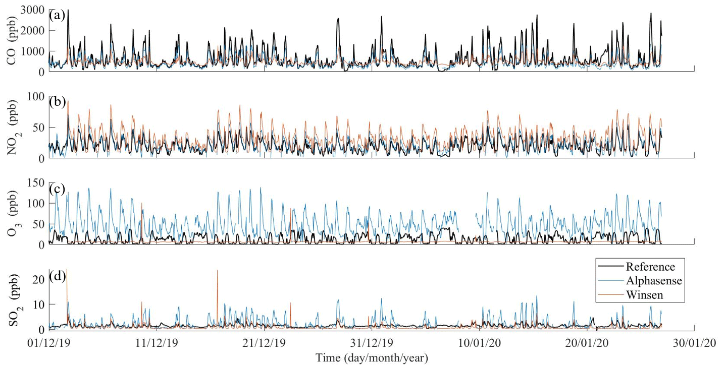
Figure 3 Time series of hourly averaged concentrations measured by the Alphasense and Winsen ECh gas sensors and the reference instruments from 1 December 2019 to 26 January 2020 for CO (a), NO₂ (b), O₃ (c) and SO₂ (d). We should note that the data from the LCSs were determined through the calibration equations discussed in Sect. 2.4 (for the Alphasense sensors) or provided directly by the sensors (for the Winsen sensors). Exceptions to this are the data from the Winsen CO LCS, for which we subtracted 400 ppb from all the measurements, and the SO₂ LCSs from both manufacturers, where the signal was divided by a factor of 10 for illustration purposes.

Aggregated statistics from all the measurements and for each sensor during the entire testing period are provided in Table 1. Overall, the CO measurements by the LCSs from both manufacturers show better agreement with those reported by the respective reference instruments (cf. mean values in Table 1) compared to the rest of the sensors tested. Both CO sensors capture the temporal concentration variability attributed primarily to the morning and afternoon traffic pollution. The Alphasense CO LCS exhibits the lowest MRE, with a value of −4.7 %, and the highest correlation (R²=0.54) compared to the respective Winsen LCS (MRE =35.1 %, R²=0.25).

Table 1 Summary statistics, including the number of hourly averaged data points used for data analysis of each LCS (N), and the mean concentration of hourly averaged gaseous concentrations measured by the Alphasense and Winsen LCSs and the reference instruments for the entire study period, together with the standard deviation for each case, as well the associated values of the MRE, MBE, MAE and R². The LoD values for each LCS are also provided for comparison. In addition, the slope and intercept of the linear regression for each sensor are given as per the US EPA (Duvall et al., 2021).

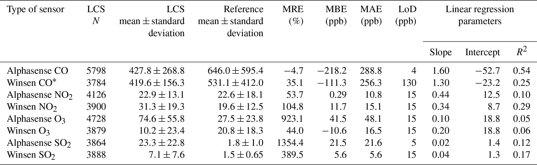
^* Measurements recorded by the Winsen CO sensors were reduced by 400 ppb in order to better match the measurements from the reference instruments. The Winsen CO statistics provided in this table correspond to the corrected data.

The measurements recorded by the NO₂ LCSs from both manufacturers followed similar temporal patterns to those of the reference instrument, exhibiting moderate, but similar, correlations (i.e. R²=0.10 for Alphasense and R²=0.29 for Winsen). Overall, both LCSs overestimated the NO₂ concentrations, with the Alphasense NO₂ sensor exhibiting better performance compared to that of Winsen, as indicated by the MRE (53.7 % against 104.8 %, respectively) and MAE (10.8 against 15.1 ppb, respectively) shown in Table 1. The higher errors associated with the NO₂ LCSs of both manufacturers can be attributed to cross-sensitivities with other gaseous pollutants.

The Alphasense O₃ sensor significantly overestimated the absolute reference concentrations, exhibiting high MRE (923.1 %) and MAE (48.1 ppb) values. On the other hand, the Winsen O₃ sensor mainly underestimated the actual concentration, exhibiting a significantly lower MRE (44.0 %) and MAE (16.5 ppb) compared to its Alphasense counterpart. The reported correlation coefficients of both O₃ sensors with the reference instruments were among the lowest of all the LCSs tested (R² was 0.05 for the Alphasense and 0.06 for the Winsen O₃ sensor).

The performance of the SO₂ sensors was the poorest compared to those of the rest of the LCSs, mainly because the concentrations at the monitoring station, as those were reported by the reference instruments, were quite low (ranging between 2 and 4 ppb during the study period) and always below the LoD of the LCSs, i.e. 5 ppb for the Alphasense and 15 ppb for the Winsen sensor.

Figure 4 shows the correlation of the measurements recorded by the Alphasense (Fig. 4a–d) and by the Winsen (Fig. 4e–h) LCSs with those provided by the respective reference instruments. The associated errors between the LCS and reference instrument measurements are provided in the supplement (see Fig. S3). The performance of LCSs appears to degrade from left to right in Fig. 4, with the CO and NO₂ exhibiting the best performance, whereas O₃ and SO₂ exhibit the worst.

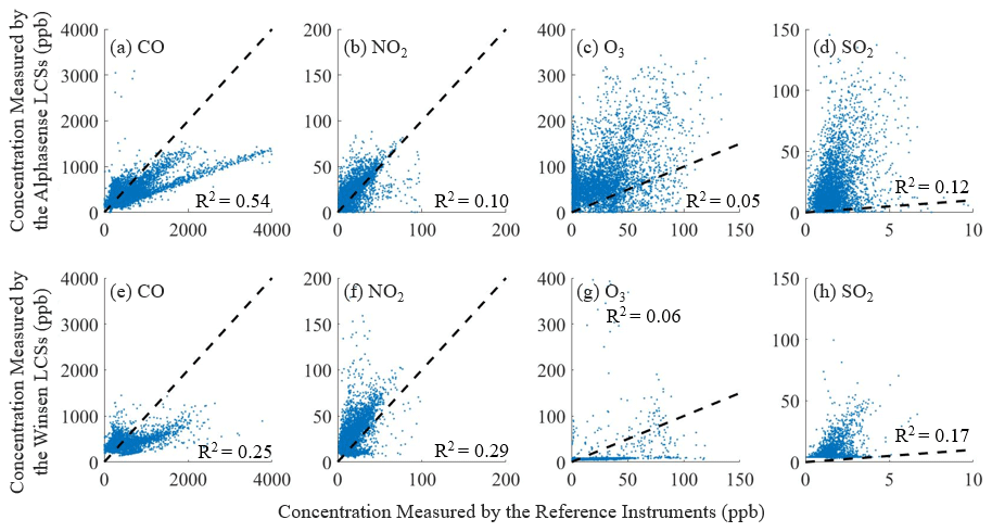
Figure 4 Correlation between the measurements recorded by the Alphasense (a–d) and Winsen (e–h) LCSs and those provided by the respective reference instruments. The dashed black lines indicate the 1:1 line. Measurements from the O₃ and SO₂ LCSs by both manufacturers do not have the same x–y-axis scales due to the big difference between reference and LCSs measurements recorded.

Two distinct linear data clusters are observed for the Alphasense CO sensor (see Fig. 4a), which can be attributed to the degradation of the sensor performance from its exposure to the high temperatures and low RH values during the summer period. This is more clearly shown in Fig. S4a, which depicts the same data tagged by the time that the measurements were recorded. We should note here that the temperatures and RH conditions that the LCSs were exposed to during the entire measuring campaign ranged from −0.4 to 42.4 ^∘C and from 2.8 % to 96.8 %, respectively. More specifically, the temperature ranged from 14.1 to 42.4 ^∘C during summer (June–August 2020) and from −0.4 to 21.3 ^∘C during winter (December 2019–February 2020), while the RH varied from 2.81 % to 95.19 % and from 32.7 % to 96.81 % during summer and winter, respectively. As discussed in Sect. 1, exposing the ECh LCSs to extreme temperature and RH conditions can cause irreversible changes in their electrolyte solution, leading to a behaviour that is noticeably different before and after that. The phenomenon is also observed for the Winsen CO LCS (see Fig. S4b), but to a lesser extent, mainly due to the limited data acquired after summer with that sensor. The same is not evident for the rest of the sensors. However, we should note here that correlation with reference instruments was not as strong in those cases, potentially due to the small extent of data clustering before and after the summer period and to the fact that the number of measurements used for the analysis was lower than that of the CO Alphasense LCS (cf. Table 1).

The data provided in Table 1 and Fig. 4 indicate that the O₃ and SO₂ LCSs by both manufacturers exhibit extremely high MREs and/or low correlations against the respective reference instruments. The high errors in the Alphasense O₃ measurement can be associated with interferences with NO₂. This is in fact taken into account, as the signal from the NO₂ LCS (mV) is subtracted from the O₃ sensor signal following the guidelines by the manufacturer (see first term in the nominator of Eq. 1). Although this correction is used for the performance analysis of the Alphasense O₃ LCS, it yields a measurement error that is higher compared to the case when the correction is not applied (cf. Fig. S6), most likely due to error propagation from the signal of the NO₂ sensors to the reported concentrations of O₃. We should note that no cross-sensitivity correction is provided by Alphasense for the case of the NO₂ sensor. It is well possible that the Winsen NO₂ and O₃ LCSs are also prone to cross-sensitivities, despite the fact that the manufacturer does not provide any information or a correction for that. Investigating that, however, is beyond the scope of this study, and thus the respective measurements were used as provided by the sensors. For the case of the SO₂ LCSs, as indicated above, most of the measurements fall below the threshold of their LoD (see Table S1). Considering the above, the performance of the O₃ and SO₂ LCSs was not assessed further, and thus we do not discuss the respective measurements from this point onwards.

3.2 Effect of temperature

Figures 5 and 6 show the correlation between the CO or the NO₂ measurements recorded by the Alphasense (Figs. 5a–d and 6a–d) and the Winsen (Figs. 5e–h and 6e–h) LCSs, with the respective measurements provided by the reference instruments at four temperature ranges: T<10, 10–20, 20–30 and >30 ^∘C. Statistics and parameters of linear regression fittings to the data at each temperature range are provided in Table 2.

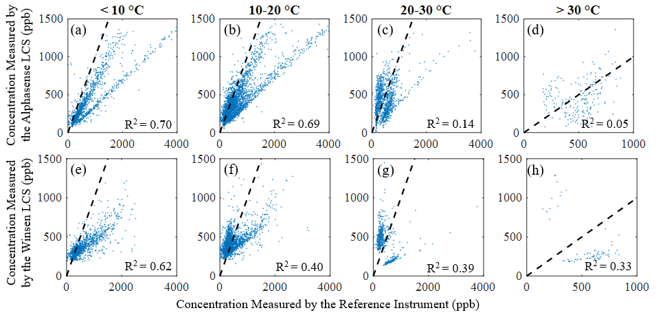
Figure 5 Correlation between the CO measurements recorded by the Alphasense (a–d) and the Winsen (e–h) LCSs and those provided by the respective reference instrument at four different temperature ranges. The 1:1 lines in each subplot are depicted as dashed lines.

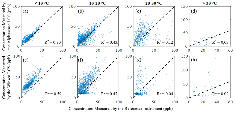
Figure 6 Correlation between the NO₂ measurements recorded by the Alphasense (a–d) and the Winsen (e–h) LCSs and those provided by the respective reference instrument at four different temperature ranges. The 1:1 lines in each subplot are depicted as dashed lines.

Table 2 Summary statistics including the number of hourly averaged data points (N) and the MRE for each LCS at four different temperature ranges over the entire study period. Linear regression parameters including NRMSE, slope, intercept and R² are also provided for each temperature range.

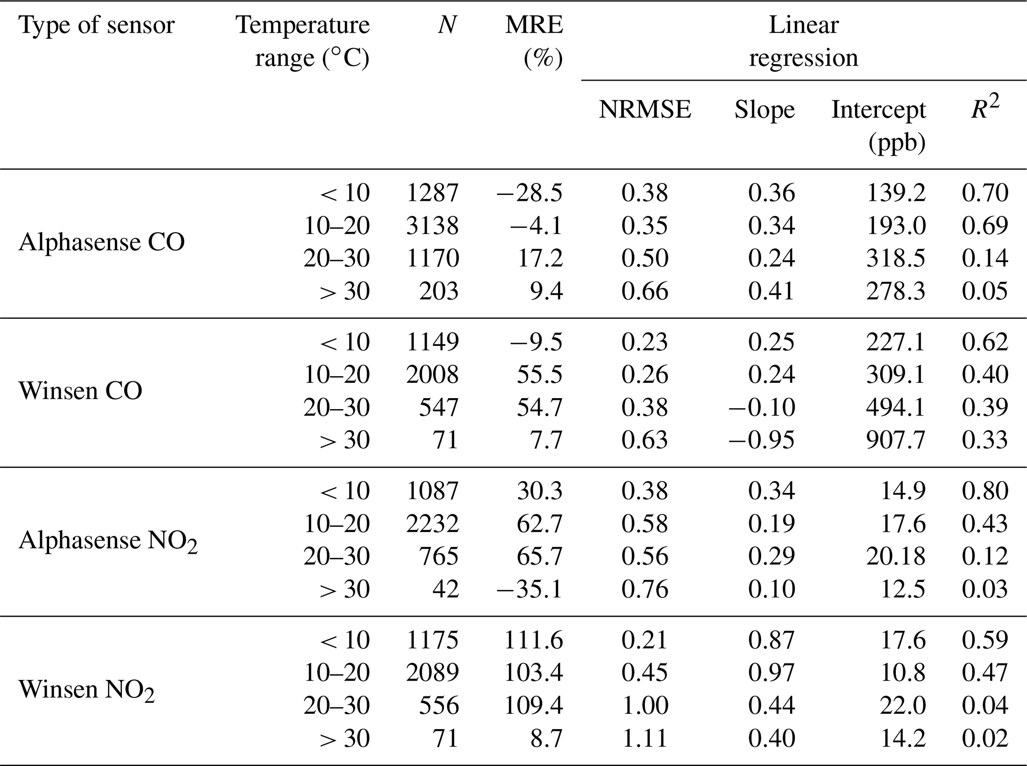
Overall, the trend is characterised by a decreasing correlation between LCS and reference measurements as the temperature increases. More specifically, the Alphasense CO sensor (see Fig. 5a–d) correlates better with the reference instrument at temperatures below 20 ^∘C than at higher temperatures (e.g. R² is 0.70 for T 10–20 ^∘C and 0.05 for T>30 ^∘C; see Table 2). Similarly, the Winsen CO sensor (see Fig. 5e–h) exhibits strong correlation with reference measurements at temperatures below 10 ^∘C (e.g. R²=0.62; see Table 2) but deteriorates at higher temperatures, exhibiting anti-correlation above 20 ^∘C (see Table 2).

The NO₂ sensors exhibit the highest correlation with reference measurements at temperatures below 10 ^∘C and the lowest above 30 ^∘C. More specifically, the Alphasense NO₂ sensor (see Fig. 6a–d) exhibits high correlations with the reference instrument (R²=0.80) below 10 ^∘C, which is similar to that of the Winsen NO₂ sensor (cf. Fig. 6e–h; R²=0.59). Above this temperature, the sensor performance deteriorates to the extent that it becomes incapable of capturing the variability in the NO₂ concentrations (cf. Fig. 6f–h). In addition to that, NO₂ LCSs can have (according to Alphasense) interferences from O₃ (Li et al., 2021), which is typically found in high concentrations during high-UV-radiation periods of the summer months in Cyprus (Vrekoussis et al., 2022), but this is not accounted for by the manufacturer, as also discussed in the previous section.

The extreme temperatures that the LCSs have been exposed to over the summer period have significantly affected their performance during the two cold periods of our tests. This is more pronounced for the CO sensors, as reflected by the two distinct data clusters in Fig. 5a and e, as well as in Fig. S4. As discussed above, this can be attributed to changes in electrolyte water content during high-temperature seasons, as in the case of the Alphasense CO LCS (cf. Sect. 3.1). It should be noted that even though the sensors were not operating during the summer months, they were exposed to ambient temperatures (up to 45 ^∘C), while their main body containing the electrolyte was at even higher values (i.e. >50 ^∘C) during midday, as a result of heat built up within the cases of the AQ monitors.

3.3 Effect of relative humidity

Figures 7 and 8, respectively, show the correlation between CO and NO₂ measurements recorded by the Alphasense and the Winsen LCSs and those provided by the respective reference instruments at four RH ranges: <30 %, 30 %–55 %, 55 %–75 % and >75 %. Statistics and parameters of linear regression fittings at each RH range are provided in Table 3.

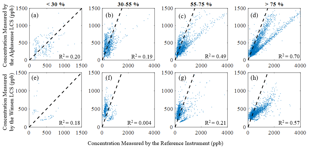
Figure 7 Correlation between CO measurements recorded by the Alphasense (a–d) or the Winsen (e–h) LCSs and those provided by the respective reference instrument at four different RH ranges. The 1:1 lines in each subplot are depicted as dashed lines.

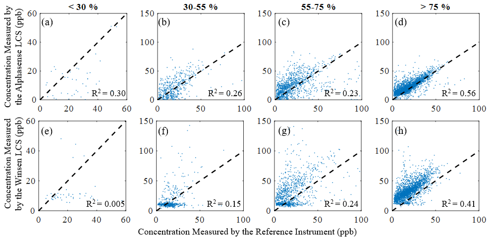
Figure 8 Correlation between the NO₂ measurements recorded by the Alphasense (a–d) or the Winsen (e–h) LCSs and those provided by the respective reference instrument at four different RH ranges. The 1:1 lines in each subplot are depicted as dashed lines.

Table 3 Summary statistics including the number of hourly averaged data points (N) and the MRE for each LCS at four different RH ranges over the entire study period. Linear regression parameters including NRMSE, slope, intercept and R² are also provided for each RH range.

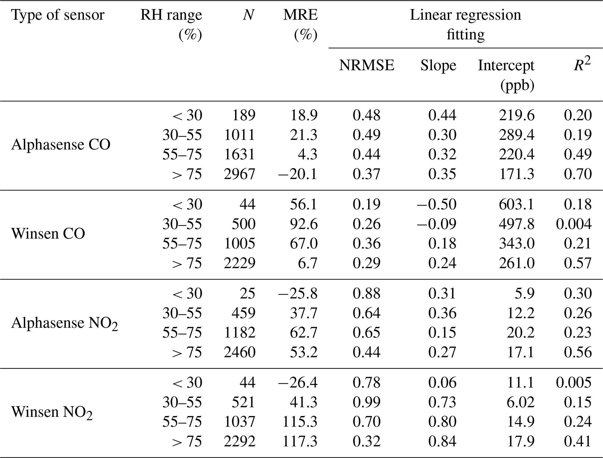
The correlation between the LCSs and the reference instruments increases with increasing RH. The Alphasense CO sensor (cf. Fig. 7a–d) correlates better with the reference measurements at RH values above 75 % (i.e. R² up to 0.70; cf. Table 3) than under drier conditions (i.e. R²=0.20 for RH <30 %; cf. Table 3). In a similar manner, the Winsen CO sensor (cf. Fig. 7e–h) exhibits strong correlation with reference measurements at RH values above 75 % (i.e. R²=0.57; cf. Table 3) but deteriorates at lower RH values.

The NO₂ LCSs from the two manufacturers exhibit the highest correlation with reference measurements at RH >75 % but decrease substantially at lower RH values. More specifically, the Alphasense NO₂ sensor (cf. Fig. 8a–d) exhibits higher correlations with the reference instrument (R²=0.56) at RH >75 %, compared to lower RH levels (i.e. R²=0.30 at RH <30 %). The measurements by the Winsen NO₂ LCS (cf. Fig. 8e–h) exhibited similar correlations with its Alphasense counterpart at RH >75 %, but its performance deteriorates at RH values below 75 % until it becomes incapable of capturing the variability in the NO₂ concentrations (cf. Fig. 8e–g). Since low RH is associated with elevated temperatures, and vice versa (cf. Fig. S5), it appears that the degraded performance noted at high temperatures for the CO and NO₂ sensors from both manufacturers corresponds to that observed under the low-RH conditions (cf. correlations provided in Figs. 5d, h and 6d, h in correspondence with those in Figs. 7a, e and 8a, e).

The Alphasense ECh gas sensors are calibrated in the lab at a fixed RH of 60 %, but according to the manufacturer they can operate in the RH range of ca. 15 % to 90 %. Long exposures of the sensors to an environment with a RH below or above 60 % can affect their performance due to evaporation or condensation, respectively, of water from/to the electrolyte (Alphasense, 2013). In principle, recalibration of these sensors would be appropriate, provided that they equilibrate to the new RH conditions. In reality, however, this is not so practical to do in the field because the period required for the sensor to reach equilibrium is much longer (ranging from a few days to almost a month) compared to the daily variability in ambient RH.

As discussed in Sect. 3.2, even though the sensors were not operating during the summer months, their main body, which was in the AQ monitors, was exposed to extreme conditions (temperatures >50 ^∘C and RH <10 %). In addition to that, the sensors were exposed to high diurnal temperature and RH variabilities, ranging from 20 ^∘C during the night to 40 ^∘C during the day, with respective values of RH ranging from 20 % to 80 % (cf. Fig. S5), and thus they never had enough time to equilibrate to any RH. These conditions had an impact on the performance of the sensors which was not only temporary (i.e. during the summer period) but persisted even after summer, as discussed above (cf. Sect. 3.1).

3.4 Degradation of low-cost ECh sensors

Figures 9 and 10 show how the measurements from the CO and NO₂ LCSs, respectively, compare with those from reference instruments over 6 consecutive days at the beginning and at the end of the measurement period. Table 4 summarises the results, providing the median MBE, MRE and NMRE, along with the temperature, RH and reference concentration corresponding to the two periods.

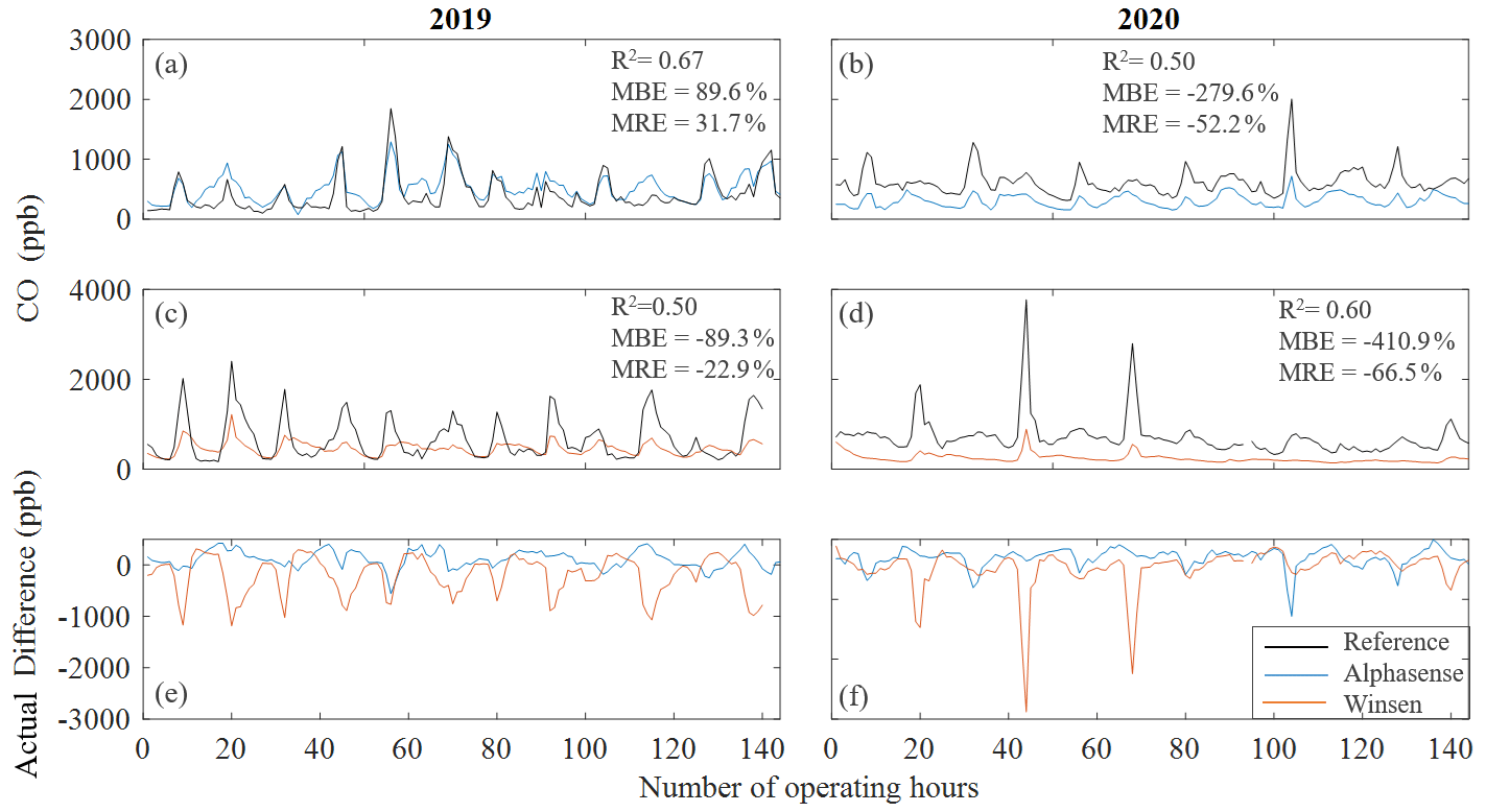
Figure 9 Time series of hourly averaged concentrations measured by the Alphasense (a–b) and Winsen (c–d) CO LCSs over 6 consecutive days at the beginning (a, c; October 2019 for Alphasense and November 2019 for Winsen) and at the end (b, d; October 2020 for Alphasense and September 2020 for Winsen) of our measurement period. The subplots in the last row show the actual concentration difference between CO LCSs and the reference instrument in 2019 (e) and 2020 (f).

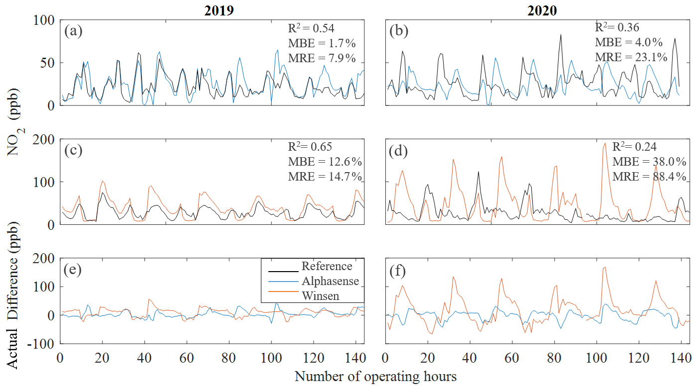
Figure 10 Time series of hourly averaged concentrations measured by the Alphasense (a–b) and Winsen (c–d) NO₂ LCSs over 6 consecutive days at the beginning (a, c; October 2019 for Alphasense and November 2019 for Winsen) and at the end (b, d; October 2020 for Alphasense and September 2020 for Winsen) of our measurement period. The subplots in the last row show the actual concentration difference between NO₂ LCSs and the reference instrument in 2019 (e) and 2020 (f).

Table 4 Median values of CO and NO₂ LCSs NMREs over 6 consecutive days at the beginning (2019) and at the end (2020) of the measurement period and the respective median values of temperature, RH and reference concentrations.

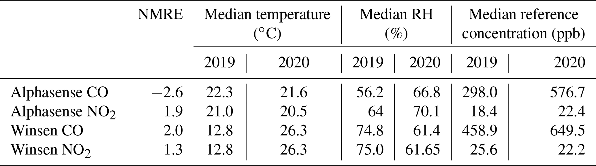
Evidently, all LCSs exhibit degradation of their performance over time, expressed as an increase in the median MBE, in terms of absolute values, after the end of our measurement period, which lasted for 1 year (cf. Figs. 9–10). Similarly, an increase in the MRE values, again in absolute terms, is also observed. For the Alphasense CO the MRE changes from almost 32 % to less than −52 % from the start to the end of the field campaign, yielding a NMRE of −2.6, whereas for the Alphasense NO₂ sensors the MRE changes from almost 8 % to around 23 %, with a NMRE of 1.9. These results are in line with those reported by Li et al. (2021), who showed that most of the Alphasense NO₂ sensors they tested exhibited significant deterioration of their performance after long-term (200 to 400 d) deployment. The Winsen LCSs exhibited similar degradation in performance, with NMRE values of 2.0 for the CO and 1.3 for the NO₂ sensors. We should note here that to make a fair comparison of the performance of each sensor at the beginning and the end of the measurement campaign, we made an effort to select measurements corresponding to similar temperature and RH conditions during the two periods. This was feasible for the datasets of the Alphasense sensors but not so easy for the Winsen, as those were not always functional after the summer period, yielding significantly fewer measurements during that period, as indicated in Table 1 and reflected by the high temperature differences in the two periods analysed here (cf. Table 4).

According to specifications provided by the manufacturers, the lifespan of ECh LCSs ranges from 2 to 3 years, and specifically for the Alphasense sensors the signal deterioration should be within less than 50 % over a period of 24 months (cf. Table S1 in the Supplement and references therein). Assessing that based on field measurements, however, is not so straightforward due to simultaneous variabilities in both the concentration of the target gases and the meteorological conditions over time. To overcome this problem, we selected two 2-month periods, one at the beginning (October–November 2019) and one at the end (November–December 2020) of our field study, constraining the temperature below 20 ^∘C and RH above 55 %, while the reference concentration for the selected data during this period was bracketed within ±10 % from the median annual reference concentration (i.e. 467.7 ppb for CO and 19.4 ppb for NO₂). By comparing the resulting Alphasense LCSs' median raw signals (i.e. V_WEu–V_AEu) at the beginning and at the end of the measurement period (cf. Fig. 11), a total drift of 86.1 mV is observed for CO and 17.2 mV for NO₂ after 1 year of operation, corresponding to drifts of 53 % and 68 %, respectively, from the initial signal of the sensors. These values significantly exceed the sensor drifts provided in the specifications of the LCSs, indicating that they increase at a rate that is more than double that suggested by the manufacturer. This discrepancy can be attributed to the high temperatures and low RHs encountered during our field evaluation, which in some cases exceeded the operational limits set by the manufacturer.

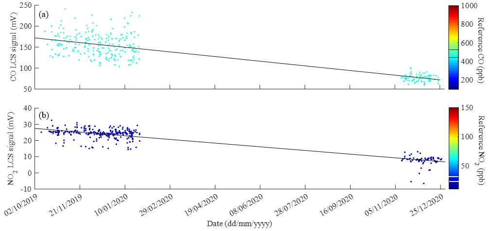
Figure 11 Signal drift of the (a) CO and (b) NO₂ Alphasense LCSs over a period of a year. The data were selected in such a way that the reference concentration is within ±10 % of the median annual reference concentration (i.e. 467.7 ppb for CO and 19.4 ppb for NO₂; cf. solid lines on colour bars), whereas the temperature and RH were constrained below 20 ^∘C and above 55 %, respectively. The solid line shows linear fitting through these measurements.

3.5 Compliance with EC guideline standards and data quality objectives

As already reported in the literature, data from LCSs do not meet the quality objectives for use in regulatory observations stated for instance by the associate EC Directive as they are not yet adequately robust and lack innate quality assurance (Peltier et al., 2020; EC, 2008). A key question, however, is whether they can still be used to provide indicative measurements, which require less accuracy and can complement the regulatory observations by increasing the spatiotemporal resolution of AQ measurements. To address this question, the sensors are required to (EC, 2008) (1) have adequate LoD for measuring concentrations below the target/limit value and even lower than the assessment threshold concentrations set by the EC guidelines; (2) provide measurements that fulfil the required minimum data capture and time coverage for indicative measurements; and (3) provide measurements that are within the minimum REU, which according to the EC legislation should remain within 25 % for the two gases that we further analyse here (i.e. CO and NO₂; cf. Sect. S6. in the Supplement for more details).

Both CO and NO₂ sensors have sufficiently low LoDs for measuring concentrations on the order of the EC threshold concentrations and even significantly below that. They can also provide rich datasets, achieving data capture and time coverage that is well above the set standard thresholds. Considering the above, the first two requirements mentioned in the previous paragraph are fulfilled, leaving the last as the main limitation for qualifying these LCSs for indicative measurements.

Figure 12 shows the REU of the measurements provided by the Alphasense (Fig. 12a–b) and Winsen (Fig. 12c–d) CO and NO₂ LCSs as a function of the respective reference concentrations. We should note here that the data were averaged over 8 h for the CO and over 1 h for NO₂ concentrations, following the EC standard for the limit values: 8600 ppb over 8 h for CO and 105 ppb over 1 h for NO₂ (EC, 2008; cf. Table S4). As shown, the sensors did not comply with the required REU limit, even at the beginning of the measurement period, when they were not affected by the summer extreme conditions. We should note here, however, that the EC limit value for CO concentrations is much higher compared to those measured at the AQ monitoring station we used in Nicosia, whereas for NO₂ they approached but never exceeded it. Nevertheless, the REU values for the two CO sensors appear to reach a plateau as the concentration of the target gas increases, which was higher for the period after the summer, and even if they are extrapolated to the limit values they would not reach the required 25 % threshold. The same is true for the Winsen but not for the Alphasense NO₂ sensor, which appears to reach this threshold at concentrations higher than ca. 70 ppb (cf. Fig. 12b), making it the only sensor that can qualify for indicative measurements according to the EC Directive.

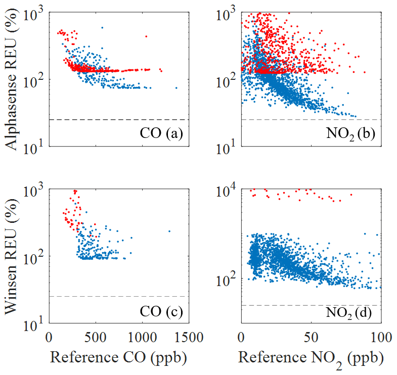
Figure 12 Relative expanded uncertainty in the 8 h averaged CO (a, c) and the hourly averaged NO₂ (b, d) measurements provided by the LCSs tested in this study. The values shown here were determined using the methodology described in the AQ Directive 2008/50/EC. The limit values suggested by the EC Directive are indicated by the horizontal dashed black line. Data shown are divided into two time periods: before (blue dots) and after (red dots) summer 2020.

4 Conclusions

We have investigated the performance of low-cost electrochemical sensors provided by two manufacturers, namely Alphasense and Winsen, for measuring the concentrations of CO, NO₂, O₃ and SO₂. To do so, we carried out yearlong measurements at a traffic AQ monitoring station in Nicosia, Cyprus, where the LCSs were collocated with reference instruments and exposed to highly variable environmental conditions, with extremely high temperatures (up to ca. 45 ^∘C) and low relative humidity (below ca. 10 %) during the summer period.

Among the different LCSs tested, the CO sensors exhibited the best overall performance, reporting measurements that had high correlation with, and low deviation from, those reported by reference instruments throughout the entire testing period. The NO₂ gas sensors from both manufacturers also exhibited good performance, having satisfactory correlations and deviations when compared to the respective reference instrument. In contrast, the performance of the O₃ sensors was not satisfactory, while the SO₂ sensors were not possible to be evaluated because the ambient concentrations were below their LoDs.

Our measurements demonstrate that the performance of the CO and NO₂ sensors from both manufactures is affected by exposure to temperatures above ca. 25 ^∘C and RH levels below ca. 55 %. This is most probably caused by the evaporation of water from the sensor electrolyte, which in turn affects the currents induced by the interaction of the target gases with the working electrodes through the cells of the sensors. After prolonged use under extreme conditions (i.e. temperatures above ca. 40 ^∘C and relative humidity conditions below ca. 10 %) the sensors exhibited high errors and in some cases technical malfunctions, making them practically unusable. Although the sensors regained their operability (i.e. being able to provide uninterrupted data) as the conditions became milder, their performance did not fully recover. Exposure of the sensors to these extreme conditions appeared to cause a signal drift of more than 50 % over a period of a year, which is more than twice as fast as that indicated by the manufacturers.

Although the LCSs tested in this work fulfilled two of the three criteria (i.e. adequate LoD, measurements that fulfil the required minimum data capture and time coverage) that qualify them for indicative measurements according to EC standards, they fail the third criterion of exhibiting REU values below 25 %. The only exception to this generalisation was the Alphasense NO₂ sensor, which exhibited REUs close to 25 % for concentrations above 70 ppb, which is below the hourly limit NO₂ value, making it the only LCS that can be used for indicative measurements according to the EC Directive.