Concept, absolute calibration, and validation of a new benchtop laser imaging polar nephelometer

Polar nephelometers provide in situ measurements of aerosol angular light scattering and play an essential role in validating numerically calculated phase functions or inversion algorithms used in space-borne and land-based aerosol remote sensing. In this study, we present a prototype of a new polar nephelometer called uNeph. The instrument is designed to measure the phase function, F₁₁, and polarized phase function, $-F_{\mathrm{12}}/F_{\mathrm{11}}$, over the scattering range of around 5 to 175^∘, with an angular resolution of 1^∘ at a wavelength of 532 nm. In this work, we present details of the data processing procedures and instrument calibration approaches. uNeph was validated in a laboratory setting using monodisperse polystyrene latex (PSL) and di-ethyl-hexyl-sebacate (DEHS) aerosol particles over a variety of sizes ranging from 200 to 800 nm. An error model was developed, and the level of agreement between the uNeph measurements and Mie theory was found to be consistent within the uncertainties in the measurements and the uncertainties in the input parameters for the theoretical calculations. The estimated measurement errors were between 5 % and 10 % (relative) for F₁₁ and smaller than ∼ 0.1 (absolute) for $-F_{\mathrm{12}}/F_{\mathrm{11}}$. Additionally, by applying the Generalized Retrieval of Aerosol and Surface Properties (GRASP) inversion algorithm to the measurements conducted with broad unimodal DEHS aerosol particles, the volume concentration, size distribution, and refractive index of the ensemble of aerosol particles were accurately retrieved. This paper demonstrates that the uNeph prototype can be used to conduct accurate measurements of aerosol phase function and polarized phase function and to retrieve aerosol properties through inversion algorithms.

1 Introduction

Atmospheric aerosol particles have a substantial impact on the Earth's radiative budget through their direct interaction with solar radiation and by affecting cloud formation processes (Boucher et al., 2013). Furthermore, aerosol particles are a significant component of air pollution, which has been estimated to cause 4.2 million annual premature deaths worldwide (Cohen et al., 2017). The complex compositional and microphysical properties and high spatiotemporal variability in atmospheric aerosols make it difficult to properly characterize them and to constrain them in atmospheric global model simulations. This leads to large uncertainties in estimation of aerosol radiative forcing contribution when compared to other prevalent climate change drivers such as CO₂ (Myhre et al., 2013). Global-scale, long-term measurements of various aerosol properties are essential for obtaining in-depth insights into atmospheric aerosol variability and for developing a more realistic parametrization of aerosol particles in global atmospheric models. Passive satellite and ground-based remote sensing, which are the main approaches used to obtain atmospheric aerosol observations on a global scale, rely on measurements of elastically scattered solar radiation by atmospheric aerosols (Boucher, 2015). Remote sensing instruments are typically designed to detect the radiance of scattered light over single or multiple angles (radiometric measurements), while certain instruments can provide complementary measurements on the scattered light polarization state (polarimetric measurements; Dubovik et al., 2019). The polarimetric and radiometric measurements contain implicit information of numerous aerosol microphysical properties such as the refractive index (RI), size, and shape (Bohren and Huffman, 2004).

In remote sensing, aerosol properties are inferred from radiometric and polarimetric measurements by using inversion algorithms (e.g., Dubovik et al., 2021). Due to the ill-posed nature of the inverse problem, the inversion algorithms often use simplified forward scattering models and a priori assumptions to be able to retrieve aerosol properties. For instance, it is common to assume a spherical shape and use the Mie theory for the forward kernel of inversion algorithms (Holben et al., 1998; Omar et al., 2009). While such an assumption is sufficient for spherical aerosols, studies have shown that light scattering by complex aerosols, such as biomass burning aerosols, is quite distinct from light scattering described by the Mie theory (Espinosa et al., 2019; Manfred et al., 2018). Hence, aerosol property retrievals from remote sensing measurements are prone to uncertainties and biases. Independent in situ validation techniques are required to identify the potential biases and uncertainties in the retrieved aerosol properties from remote sensing measurements (Mishchenko et al., 2007). Direct validation of remote sensing measurements is a challenging and expensive task that often involves airborne measurements (Schafer et al., 2019). Alternatively, mimicking atmospheric remote sensing measurements with in situ instruments enables the validation of remote sensing retrieval algorithms in laboratory environments (Schuster et al., 2019). This is a more cost-effective approach compared to the direct validation of atmospheric aerosol retrievals and allows for the testing of aerosol samples with well-defined properties.

Polar nephelometers are in situ instruments primarily designed for radiometric measurements. Following the Stokes formalism, polar nephelometers measure the F₁₁(θ) element of the aerosol scattering matrix F(θ) over multiple scattering polar angles θ (Espinosa et al., 2017). The F₁₁(θ) element is also referred to as the phase function (PF) and describes the partial scattering coefficient of an aerosol as a function of θ for non-polarized incident light. A subset of polar nephelometers is also capable of performing polarimetric measurements that is additionally providing the polarized phase function (PPF), $-F_{\mathrm{12}}\left(\mathit{\theta }\right)/F_{\mathrm{11}}\left(\mathit{\theta }\right)$, which describes the relative degree and orientation of linear polarization of scattered light as a function of θ for non-polarized incident light (e.g., Dolgos and Martins, 2014).

Polar nephelometers have a long history (e.g., Waldram, 1945), and over the years, several different instrument designs have been introduced. Broadly, polar nephelometer designs can be categorized into three groups (Barkey et al., 2012). Goniometer-type nephelometers conduct radiometric and polarimetric measurements using a detector mounted on a rotatable arm (Li et al., 2018; Horvath et al., 2018; Waldram, 1945). These instruments can achieve high angular resolution at the expense of a relatively low time resolution. Multidetector-type nephelometers use sensors mounted at fixed scattering angles (Barkey et al., 2007; Dick et al., 2007; Nakagawa et al., 2016). These instruments can provide rapid radiometric and polarimetric measurements, while the number of probed scattering angles remains limited. Laser-imaging-type nephelometers image the light scattered by an ensemble of aerosol particles within a laser beam onto a charge-coupled device detector (CCD), such that scattering angle and position on the image are unambiguously related. These instruments can provide radiometric and polarimetric measurements with high angular resolution and high time resolution. While more sophisticated polar nephelometers capable of measuring more components of F(θ) exist (Muñoz et al., 2012; Hu et al., 2021), the majority of the polar nephelometers used in atmospheric applications typically measure either PF only or PF and PPF. Polarimetric data provided by these instruments make it possible to retrieve aerosol properties using similar inversion schemes (e.g., Espinosa et al., 2019; Schuster et al., 2019; Boiger et al., 2022).

In spite of several advantageous features, the use of laser imaging nephelometers has been quite limited. One of the earliest versions is the polarized imaging nephelometer (PI-Neph) that was introduced by Dolgos and Martins (2014). The PI-Neph provides both radiometric and polarimetric measurements at three wavelengths over an angle range of 3 to 177^∘, with angular resolution of 1^∘. This instrument has been deployed in airborne field campaigns. For example, Espinosa et al. (2017) applied the Generalized Retrieval of Aerosol and Surface Properties (GRASP), which is a well-established retrieval algorithm, to measurements conducted by the PI-Neph and successfully retrieved size distribution, RI, and shape properties of aerosol particles.

Since the inception of the PI-Neph, several other laser imaging nephelometers have been introduced. For instance, Bian et al. (2017) and Manfred et al. (2018) used laser imaging nephelometers with only radiometric capabilities to measure the PF of ambient aerosol particles and biomass burning aerosols, respectively. More recently, Ahern et al. (2022) introduced a laser imaging nephelometer capable of conducting simultaneous polarimetric and radiometric measurements at two distinct wavelengths, which is suitable for deployment on aircraft.

In this study, a new laser-imaging-type nephelometer, referred to as uNeph, was designed and constructed jointly by Micos Engineering GmbH (Dübendorf, Switzerland) and the Laboratory of Atmospheric Chemistry at the Paul Scherrer Institute (PSI; Villigen, Switzerland). Considerable downsizing was a design goal for uNeph to facilitate the deployment and operation of the instrument in different settings. This work presents uNeph, including an instrument description and the experimental setup (Sect. 2), basic data processing procedures (Sect. 3), and signal calibration approaches and error assessment (Sect. 4), in addition to validation and a first basic application (Sect. 5).

2 Instrument description and experimental setup

2.1 uNeph

uNeph is a benchtop laser imaging polar nephelometer. It consists of an optical box with dimensions $\mathrm{44}\times \mathrm{61}\times \mathrm{18}$ cm and personal computer (PC), in addition to a few small control boxes kept externally. A schematic of the key elements of the uNeph instrument is shown in Fig. 1. A solid-state continuous wave laser provides linearly polarized light at 532 nm (∼ 200 mW). The laser beam is collimated with a Gaussian size around 1 mm and vignetted with apertures to slightly cut it down to ∼ 0.5–1.0 mm. Exchangeable neutral-density (ND) filters are utilized to reduce the laser intensity in order to adjust the instrument sensitivity to different levels. We particularly used three different optical density filters throughout the experiments (Thorlabs, Inc., Newton, NJ, USA; models NE10A, NE15A, and NE20A, with optical density levels of 1, 1.5, and 2.0, respectively).

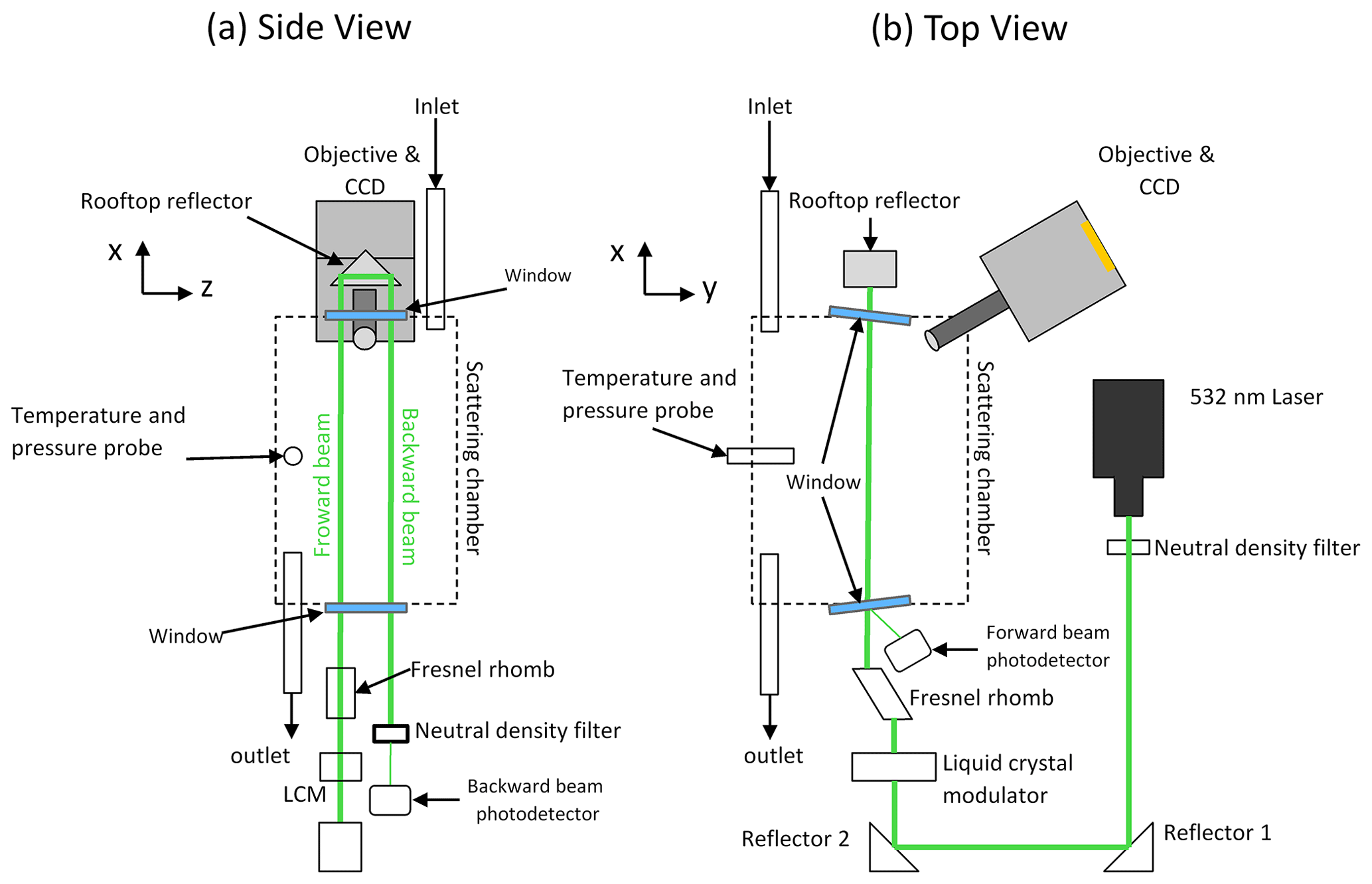
Figure 1 (a) Side view and (b) top view schematics of the uNeph instrument (the drawing is not to scale).

The next elements serve to rotate the angle of the linear polarization state, following the approach detailed in Dolgos and Martins (2014). It is an assembly consisting of a liquid crystal variable retarder (LCVR) and a Fresnel rhomb, which acts as a quarter-wavelength retarder. Subsequently, the beam is passed through multiple irises to adjust the cross-sectional area of the beam and to reduce the level of undesired background light (e.g., stray light) in the scattering chamber (not shown in Fig. 1).

The laser beam is directed through a scattering chamber twice, using a rooftop reflector in between (this is a rooftop design that maintains the linear polarization nature of the laser beam). The input window of the scattering chamber is placed at angle, and the small reflected part, not blocked by the antireflection (AR) coating, is used to measure the input laser power (forward beam) with a photodetector (Si free-space amplified photodetector; Thorlabs, Inc., Newton, NJ, USA; model PDA100A2). The power of the backward beam exiting the chamber after both passages is also measured with a second similar photodiode (a ND filter is used for protection). Since the laser intensity attenuation is expected to be minimal within the range of aerosol sample concentration tested in this study, we only used the forward beam laser power measurements to compensate the raw signals for variations in laser intensity.

The scattering chamber, also shown in Fig. 1, serves as the measurement cell. It is a metal chamber with a length of ∼ 30 cm and a volume of ∼ 2.5 L. The laser beam enters and leaves the cell through sealed windows. The chamber has a removable lid, which enables access to the beam path, e.g., for performing calibration tasks. A pressure (p), temperature (T), and relative humidity (RH) sensor is mounted inside the scattering chamber. A sample inlet and outlet are installed at opposite ends of the scattering chamber to flush it continuously with gas or aerosol samples. A detection unit consisting of an optical objective and a camera is used to collect the scattered light. Light scatters inside the forward and backward beams in forward (scattering angles; $\mathrm{0}{}^{\circ }\le \mathit{\theta }\le \mathrm{90}{}^{\circ }$) and backward ($\mathrm{90}{}^{\circ }\le \mathit{\theta }\le \mathrm{180}{}^{\circ }$) directions, respectively, and appears as two distinct stripes on the camera image (Fig. 2a). The camera is an Ar-filled, actively cooled, monochrome, charge-coupled device (CCD), with a resolution of 1392×1040 pixels (9×6.7 mm sensor size and 6.45×6.45 µm pixel size) and a 16 bit analog-to-digital (A/D) converter (TRIUS PRO825; Starlight Xpress Ltd.). A three-dimensional scheme of the laser path within the scattering chamber is demonstrated in Fig. S1. One design element of uNeph is the use of a wide field of view pinhole lens in the camera objective, which enables the instrument to be downsized. The camera objective is the Marshall V-PL25CS-12 (discontinued), with a pinhole size of ∼ 2 mm, a focal length of 2.5 mm, and an aperture of F2.8. The field of view (diameter) is 100^∘. Direct connection of the CS-mount objective to the cooled CCD is not possible, and therefore, a Thorlabs, Inc., re-imager optical system is needed. The objective is placed at 45^∘ from the direction of the beams, with the pinhole being placed between both beams (as depicted in Fig. S1 in the Supplement). Based on the geometry (Fig. S1), the pinhole and a given laser beam define a scattering plane. The forward and backward laser beams were aligned to be parallel, and the pinhole location was adjusted such that the two scattering planes have 45^∘ (forward beam) and 135^∘ (backward beam) orientations relative to the y–z plane (as depicted in Fig. S1b). They are chosen to be perpendicular to each other to achieve an identical angle between the scattering plane and orientation of linear polarization state for both forward and backward beams. Two distinct linear polarization states, e.g., with nominal orientation that is either in parallel or perpendicular to the scattering planes, are sufficient to measure the phase function and polarized phase functions (see Sect. 4.1). A polarimeter (PAX1000VIS/M; Thorlabs, Inc.) was used, in a setup without the chamber, to verify that the forward and backward laser beams are almost fully linearly polarized. The set points of the LCVR to achieve parallel or perpendicular linear polarization relative to the scattering plane were determined by inserting an additional linear polarizer in front of the chamber. Its orientation was chosen to be perpendicular to the nominal laser polarization orientation, and then the LCVR setting was varied to achieve minimal beam transmission. Uncertainties in the pinhole alignment relative to the laser beams are estimated to have larger effects on the deviations from the nominal linear polarization than the quality of polarization control. We use subscripts “1” and “2” to denote the nominal parallel and perpendicular linear polarization operation set points, respectively. The raw data provided by uNeph consist of a digital image of the light scattered from the forward and backward beams at a given state of polarization. When conducting measurements, a defined polarization state is first applied, followed by acquisition of an image (or multiple images) at a specified exposure time, t_expo. Auxiliary sensor readings (T, p, RH, and photodetectors) are simultaneously being logged. Figure 2a shows an example of a raw light scattering image for a particle-free air sample taken at polarization state 2, i.e., nominally perpendicular linear polarization. Further data processing will be explained in Sect. 3 onwards.

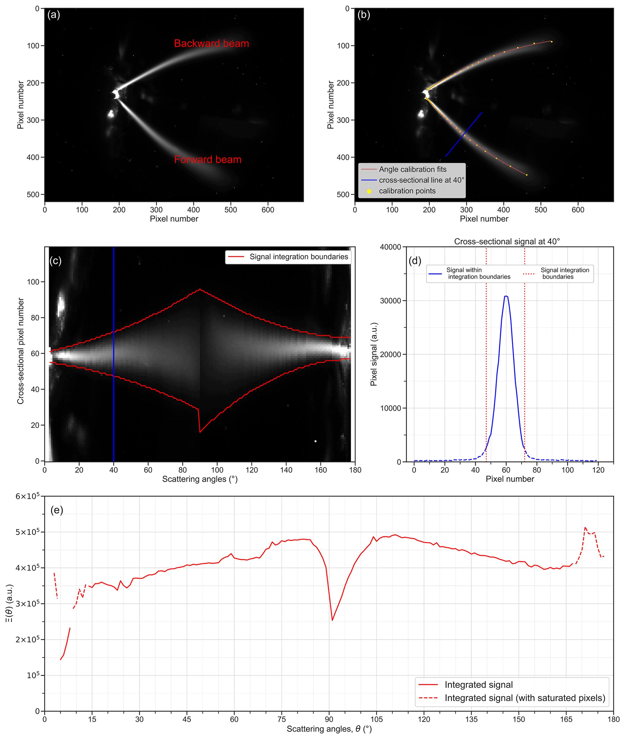
Figure 2 (a) Example of a raw sample image of the particle-free air acquired at perpendicular polarization, with an exposure time of 215 s. (b) The angle calibration fit lines (red) and an example cross-sectional line (blue) indicate pixels corresponding to a scattering angle of θ=40^∘. (c) Light scattering image after transformation to pixel angle coordinates. (d) Cross-sectional signal for the example θ=40^∘. (e) The integrated light scattering signal, Ξ, over measured scattering angles, θ, for a particle-free air sample.

2.2 Experimental setup for uNeph calibration and validation

Some uNeph calibration measurements rely on probing pure, particle-free gases, following the experimental setup shown in Fig. 3a. For this purpose, particle-free air, CO₂, Ar (argon), or He (helium) was flushed through the uNeph, with a flow rate of ∼ 5 L min⁻¹. Further calibration and validation measurements were done using aerosol samples with well-defined properties, using the experimental setups shown in Fig. 3b or c to generate quasi-monodisperse or broad unimodal aerosol samples, respectively. Initial aerosol generation steps were identical for these two types of experiments. The aerosol samples used in this study were spherical polystyrene latex size standards (PSL; see Table S1 in the Supplement for specifications) and di-ethyl-hexyl-sebacate (DEHS). DEHS is a non-absorbing oil-like liquid, hence also resulting in spherical aerosol particles.

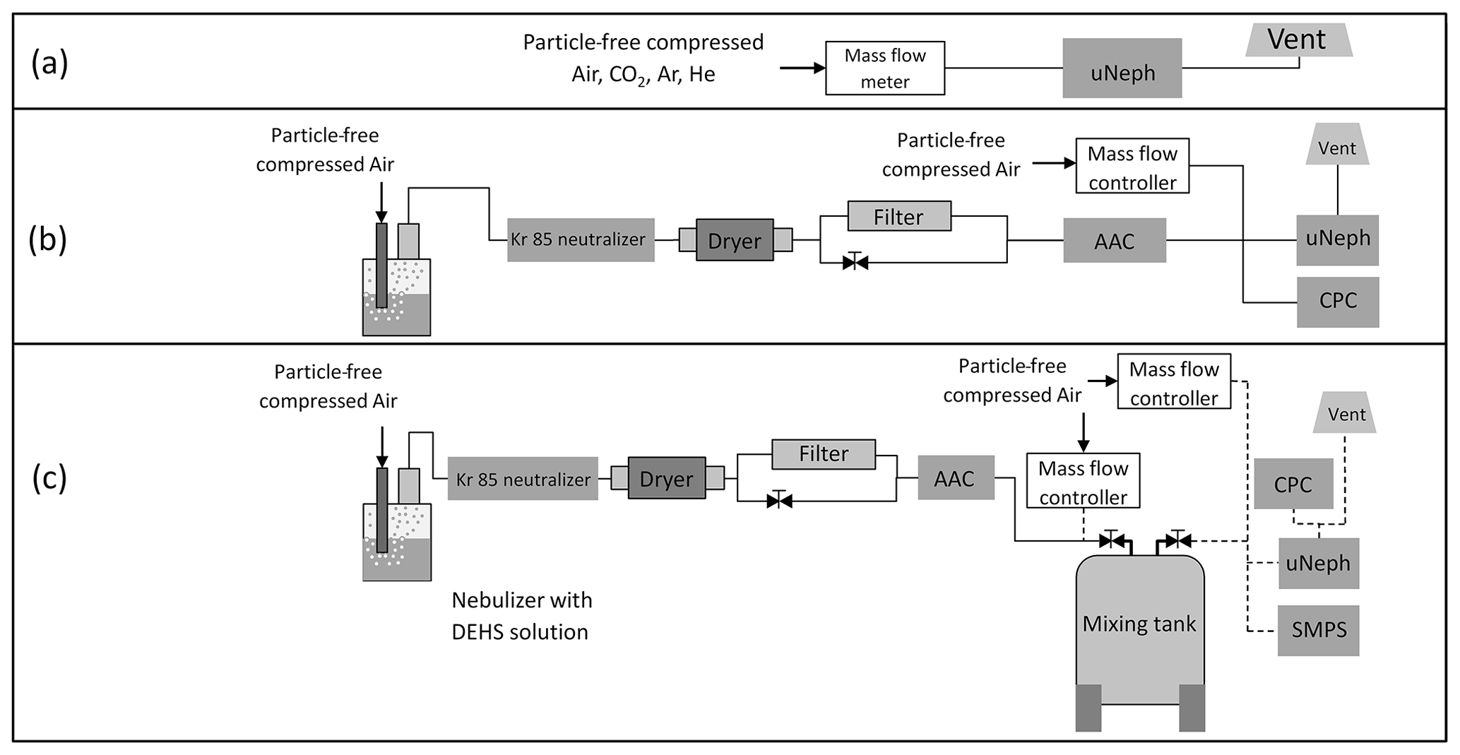
Figure 3 Schematics of experimental setup for probing (a) gases, (b) quasi-monodisperse aerosol, and (c) broad unimodal aerosol. The aerosol generation step (solid lines) and the sampling step (dashed lines) shown in panel (c) were performed in sequence as described in the main text.

PSL suspensions diluted with Milli-Q water were nebulized using a commercial atomizer aerosol generator (ATM 226; Topas GmbH, Dresden, Germany). Liquid DEHS in a pure form was aerosolized using a Collison-type nebulizer (CH Technologies, Westwood, NJ, USA). After particle generation, aerosol samples were passed through a Kr-85 neutralizer to mitigate the aerosol electrostatic losses in the sampling line. Subsequently, to remove water content from the nebulized aerosol particles, the sample flow was passed through a silica gel diffusion dryer. A dilution stage was placed after the dryer to adjust the aerosol concentration to suitable levels, particularly during the tests with DEHS for which the initial particle number concentrations were typically too high. Next, a quasi-monodisperse size cut was extracted from the sample flow by directing it through an aerosol aerodynamic classifier (AAC; Cambustion Ltd, Cambridge, UK; Tavakoli and Olfert, 2013). The major advantage of the AAC is that the size selection only depends on the particle aerodynamic diameter, while being independent of the charge; i.e., there is no interference from larger particles carrying multiple charges. For PSL aerosol experiments, the AAC was operated at a resolution parameter set point of 10, and the nominal diameter set point of the AAC was adjusted to maximize the particle number concentration downstream (i.e., at the peak of the PSL size mode). This approach ensures that unwanted small residual particles from solutes in the suspension and possible agglomerated multiplets are removed without causing a shift in the modal size of the selected PSL particles. The AAC set point diameters which maximized PSL transmission agreed to within 1 % of the calculated aerodynamic diameters of the PSL size standards (Table S1), which validates accuracy of size selection by the AAC. For the DEHS aerosol experiments, the AAC was operated at a resolution parameter set point of 20 to provide a quasi-monodisperse DEHS aerosol of a known size. The AAC aerodynamic diameter set points and corresponding volume equivalent diameters are included in Table S2. In all the tests, the sample flow through the AAC was ∼ 1 L min⁻¹. Up to this point, the particle generation and selection have been identical for all aerosol experiments. For the monodisperse test experiments (Fig. 3b), the size-selected aerosol sample was combined with a stream of particle-free compressed air, which was maintained at ∼ 4 L min⁻¹, before being sent to the uNeph and a condensation particle counter (CPC; TSI Incorporated, Shoreview, MN, USA; model 3776) that operated in parallel. This provides phase function measurements for an aerosol of a known refractive index (RI) and size and number concentration.

The experimental setup was slightly modified to generate and probe a broad unimodal aerosol with larger but still moderate width for the size distribution (Fig. 3c). A holding container (with volume of ∼ 100 L) was placed after the aerosol classification stage. The AAC was stepped through six different set points ranging from 310 to 450 nm aerodynamic diameters, while filling the container in flow-through mode over a time period of ∼ 10 min. Afterwards, the outlet valves were closed for ∼ 18 h to allow the size distribution to become more homogeneous through mixing and coagulation. After the coagulation process, the sample was slowly pushed through the outlet of the holding container by applying a particle-free airflow of 0.5 L min⁻¹ at the inlet. The extracted aerosol sample was diluted with 4 L min⁻¹ particle-free air and then distributed to the aerosol instruments. In addition to the uNeph and the CPC, a scanning mobility particle sizer (SMPS) was employed to measure the aerosol number size distribution. The SMPS was a combination of a differential mobility analyzer (DMA; TSI Incorporated, Shoreview, MN, USA; model 3082) and a CPC (TSI Incorporated, Shoreview, MN, USA; model 3775).

3 uNeph data processing

Deriving calibrated and polarized phase function data from the uNeph raw digital images requires many intermediate data processing steps. The two main stages are image data reduction and angular signal processing, as delineated in the flowcharts (Fig. S2) and detailed in the following.

3.1 Image data reduction

3.1.1 Dark signal corrections

Digital images acquired by the CCD contain some signal that is entirely unrelated to actual illumination of the CCD, which is hereafter referred to as the dark signal. It can be characterized by acquiring images without illuminating the CCD (Manfred et al., 2018; i.e., with the uNeph laser turned off). The CCD also has a few hot pixels that possess an abnormally large dark current (e.g., Fig. S3). Image processing, which follows the flowchart in Fig. S2a, starts with hot-pixel identification and removal (Fig. S2a), as detailed in Sect. A1. The subtraction of the dark signal contribution, as detailed in Sect. A2, comes next. The dark signal itself has two systematic contributions, a positive bias (constant) and dark current (proportional to exposure time), in addition to superimposed random noise. Accordingly, the two constants are sufficient for characterizing the systematic components of the dark signal as a function of the exposure time (Eq. A2). Figure S4 demonstrates that this correction approach works well to subtract the dark signal contribution with small residuals.

3.1.2 Scattering angle calibration

The relationship between scattering angle and image pixels is determined through the scattering angle calibration, which is described in more detail in Sect. A3. Briefly, this is achieved by relating an axial position inside the laser beam with both the scattering angle and the corresponding image pixel coordinates. For this purpose, a pinhead mounted on a 3D translation stage is placed at 27 different positions inside the forward and backward laser beams (Figs. S5 and S6). An image of the diffused laser light is recorded, along with the corresponding coordinates of the pinhead position. Figure S5b illustrates how the laser beam axis, the pinhead position (S), and the center of the pinhole objective (P) define the scattering angle (θ). The center of the pinhole objective P is not known exactly, which introduces uncertainty into θ, as explored and discussed in Sect. 4.3. The center of the bright spot on the image provides the corresponding pixel (Fig. S6a). This calibration step ultimately provides a list of pixel coordinates along the centerline of the forward and backward beams, together with the corresponding scattering angles. Such calibration points are shown in Fig. 2b as yellow dots, along with a second-order polynomial fit curve through them (red curve).

3.1.3 Angular signal extraction

The laser beam stripes on the image are wider than just one pixel (e.g., Fig. 2b). Limiting further data analysis steps to the centerline pixels would impose an unnecessarily high statistical noise on the results (Ahern et al., 2022). Therefore, the next steps, following the flowchart shown in Fig. S2a, aim at integrating the raw image signal along the beam cross section for each angle.

The image is first transformed to bring the laser beam stripes on a straight line in parallel to the new abscissa representing scattering angle. The top (backward beam) and bottom (forward beam) halves of Fig. 2b are separately transformed and stitched together with a common abscissa, as shown in Fig. 2c. The blue lines in Fig. 2b and c illustrate the beam cross section at θ=40^∘ before and after transformation, as an example. Section A4 provides a more detailed description of the image transformation. A regular grid with 1^∘ angular resolution was chosen for the extracted image. No attempts were made to extract the signal with a higher angular resolution, given that the information content of the measured phase functions is often limited by measurement uncertainties rather than by the angular resolution. The transformed image signal is then integrated along the beam cross section for each angle (illustrated in Fig. 2d for θ=40^∘, as an example). Integration boundaries were chosen to maximize the ratio of the actual light scattering signal to the interfering signal contributions, such as stray light or dark current residuals. Specifically, we chose the integration limits, indicated by red lines in Fig. 2c and d, at the pixels where the signal drops to ∼ 10 % of the peak signal at the beam center (see Sect. A4 for details). Integration at each angle provides, at the end of the flowchart shown in Fig. S2a, an angle-dependent scalar value, which represents the raw angular signal, Ξ(θ) (Fig. 2e).

3.2 Angular signal processing

3.2.1 Selection of valid signals

The initial data processing steps described in Sect. 3.1 serve to provide a signal that is, ideally, strictly proportional to the image exposure time and without offset. Two signals, Ξ₁(θ) and Ξ₂(θ), obtained when probing a stable homogeneous scattering medium with two different exposure times, t_expo,1 and t_expo,2, respectively, are expected to fulfill the following:

$$\begin{array}{}\text{(1)}& {\mathrm{\Xi }}_{\mathrm{2}}\left(\mathit{\theta }\right)={\mathrm{\Xi }}_{\mathrm{1}}\left(\mathit{\theta }\right)\times t_{\mathrm{expo},\mathrm{2}}/t_{\mathrm{expo},\mathrm{1}}.\end{array}$$

In practice, this proportionality relation deteriorates at signals that are too small, when the residuals of the dark signal become relevant, or at signals that are too high, when saturation occurs. Therefore, the data processing contains a step to discard invalid signals outside the strictly proportional range (see the flowchart in Fig. S2b). To estimate the valid signal range across which proportionality holds, we measured particle-free air for 12 different t_expo values, covering the range from 0.1 to 464 s. We calculated the expected t_expo dependence of the angular signal, denoted as Ξ_exp(θ,t_expo), assuming that Eq. (1) holds and choosing the largest valid signal below the onset of saturation as a reference point. This allows the testing of the proportionality to t_expo by comparing the actual measured signal, denoted as Ξ_meas(θ,t_expo), against Ξ_exp(θ,t_expo), as shown in Fig. 4a for θ=50^∘. This demonstrates that proportionality is fulfilled in principle. Only a more precise assessment done in Fig. 4b, which presents the relative deviation $\frac{{\mathrm{\Xi }}_{\mathrm{meas}}-{\mathrm{\Xi }}_{\exp }}{{\mathrm{\Xi }}_{\exp }}$, reveals the limits of proportionality. Systematic low bias due to saturation occurs for $\mathrm{\Xi }\gtrsim \mathrm{7}\times {\mathrm{10}}^{\mathrm{5}}$. Bias also increases for very low signals; e.g., relative deviation exceeds 5 % for $\mathrm{\Xi }\lesssim \mathrm{2}\times {\mathrm{10}}^{\mathrm{3}}$ in this example. Detailed results for a wide range of angles are shown in Figs. S8 and S9 for proportionality tests with cooled and uncooled CCD, respectively. Generally, proportionality was fulfilled down to lower values of Ξ when cooling the CCD, due to the smaller residuals of the dark signal subtraction (Fig. S10).

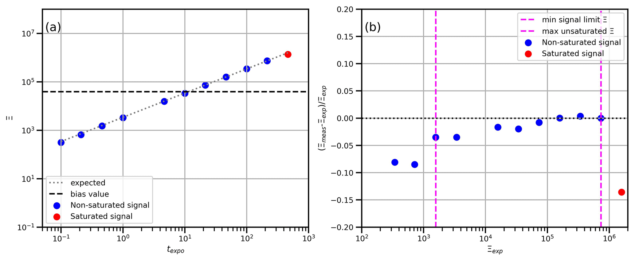
Figure 4 Panel (a) shows $\mathrm{\Xi }(\mathit{\theta }=\mathrm{50}{}^{\circ })$ vs. t_expo for air sample at polarization state 1 collected over different exposure times with CCD cooling turned on. Panel (b) shows the error of Ξ_meas relative to Ξ_exp as a function of Ξ_exp.

Figure S11 shows the repeated measurements of particle-free air samples taken over a wide range of exposure times. The two panels with the longest exposure times (bottom right) demonstrate how the upper limit (saturation) of the analog-to-digital converter leads to the capping of the signal (red line) in the center part of the beam cross section, which causes a systematic low bias in the integrated value (blue marker; right axes). At all other exposure times (t_expo≤100 s), the integrated signal has a high precision (blue markers and error bars), though random noise does become important at t_expo≲1 s (for particle-free air at the considered scattering angle).

The above results from testing the proportionality of the signals to t_expo were used to define the lower and upper limits of raw Ξ, outside of which the signals are discarded. We only retain signals for which the relative deviation remains below ∼ 6 % (lower limit) and for which no saturated pixel occurs (upper limit). Applying these strict limits approximately leaves a dynamic range of ∼ 2–3 or ∼ 1–2 orders of magnitude for cooled or uncooled CCD, respectively (Fig. S10).

Unfortunately, 3 orders in magnitude for the dynamic range may not be sufficient to operate the uNeph with a fixed t_expo, as the signal strength can vary over an even wider range, depending on scattering angle, polarization setting, and sample properties. For example, the signal at around 90^∘ drops to very low values, compared to the forward or backward scattering when applying parallel polarization to a Rayleigh scatterer, or forward scattering can exceed the backward scattering by orders of magnitude for large particles. When measuring the aerosol samples, an additional and considerable variation in the signal Ξ can occur due to the statistical fluctuations in the number of particles present inside the laser. Figure 5a–c present the data from the measurements with a high product of the DEHS particle number concentration and exposure time. This results in a smooth appearance of the light scattered out of the laser beam and onto the CCD camera (Fig. 5a) and a low level of random noise of the repeated measurements (represented by the spread of the gray curves in Fig. 5b). Consequently, the histogram of the repeatedly measured Ξ values for the aerosol sample (blue bars in Fig. 5c) has a narrow width. This implies that the mean number of particles present in the sensitive volume of the laser for this angle during image exposure is similar for all repeats, with little statistical fluctuation. The mean value of Ξ is much higher for the aerosol sample compared to the particle-free air sample shown for comparison (red bars) because the aerosol scattering coefficient clearly exceeds the air scattering coefficient at this particle size and concentration.

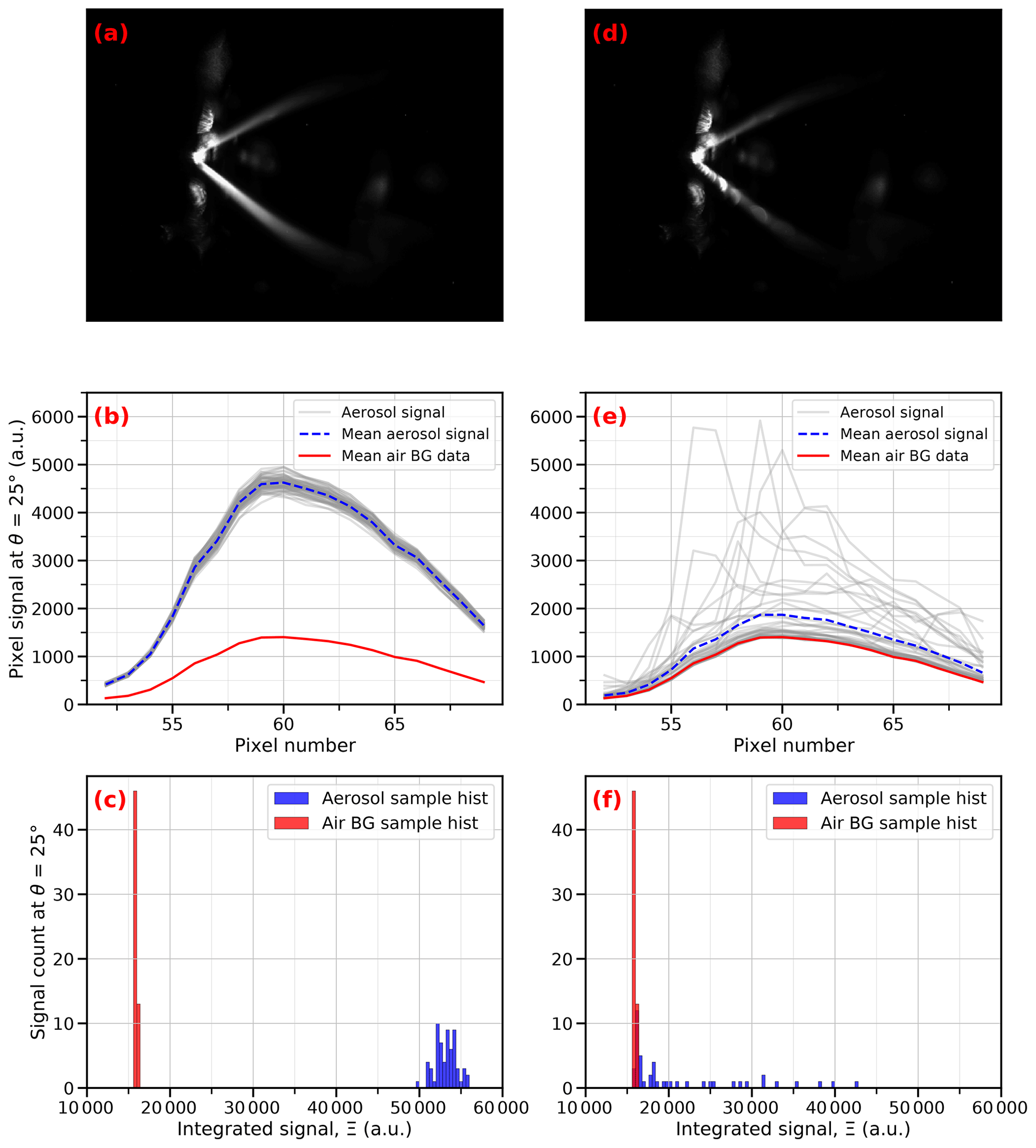
Figure 5 Panels (a) and (d) are examples of a single frame of raw data captured by uNeph at t_expo=4.64 s for 200 nm DEHS aerosol samples, with particle number concentrations of 1000 and 1 #/cc (particles per cubic centimeter), respectively. Panels (b) and (e) are the signals in a cross-sectional pixel at scattering angle of 25^∘ for the 200 nm DEHS aerosol samples, with particle number concentrations of 1000 and 1 #/cc, respectively. The gray lines are the aerosol samples in each sample frame (64 sample frames for panel b and 47 sample frames for e), the blue line is the mean of the aerosol signals, and the red line is the mean of background (BG) air (60 sample frames, with t_expo=4.64 s). Panels (c) and (f) are the histogram of the integrated signal Ξ_air (red) and Ξ_aerosol (blue) over the sampled frames for 200 nm DEHS aerosol samples, with particle number concentrations of 1000 and 1 #/cc, respectively.

In contrast, Fig. 5d–f show the results for an identical aerosol sample to the one seen in Fig. 5a–c, except for the DEHS particle number concentration being a factor of 1000 lower. In this example, the product of the particle number concentration times the exposure time is small enough to cause inhomogeneous signals. The stripes in Fig. 5d are not smooth anymore, and instead, bright spots along the laser beam become discernible. These are caused from single particles crossing the beam during image exposure. Accordingly, the signal along the beam cross section also has high fluctuations between repeats (spread in the gray lines in Fig. 5e). In some repeats, the signal remains at the background level caused by Rayleigh scattering at the air molecules (red line) across the entire beam cross section or portions of it. The histogram of the Ξ values shows that the aerosol sample signal (blue bars in Fig. 5f) is identical to the air background (red bars) for a large fraction of the images because no particle crosses the laser beam at this angle during the exposure. A subset of the Ξ values is considerably larger, corresponding to cases in which a particle is present during the exposure. For this example, the minimal and maximal signals of single images differ by a factor of ∼ 3 due to the random fluctuations caused by limited particle statistics. This problem can be mitigated by averaging a sufficiently large number of images with an identical exposure time (dashed blue line in Fig. 5e).

Given this issue of sample homogeneity, probing the full phase function with small random noise may make it necessary to measure with different exposure times and to include repeats at each of them. A condition for obtaining an unbiased average is that all repeats taken at a given t_expo fall within the proper signal range for a given angle. If some repeats were falling outside the proper signal range for a given angle, then the average would likely be biased. No bias is expected if either all images are retained or all invalid images are discarded at that angle. Therefore, all measurements taken at a t_expo with some invalid signals are to be excluded from further data analysis. Discarding data outside proper signal range is implemented as the first data processing step, starting from the integrated signals Ξ (see the flowchart in Fig. S2b).

In the presence of large particles, the data filtering step may disqualify all t_expo values. This is due to the fact that the difference in signal with or without a particle present in the laser beam becomes increasingly large with the increasing particle size. Above a certain size, this difference can exceed the proportional range of the instrument, such that it is not possible to find an exposure time for which all signals are unbiased. At longer t_expo, images with particles present suffer from saturation. At shorter t_expo, images without particles present fall below the proper signal range.

One approach to mitigate the unresolvable t_expo trade-off is to reduce the instrument sensitivity by, e.g., reducing the laser power with a stronger ND filter. This would allow for longer t_expo without exceeding the saturation limit. Longer t_expo reduces signal fluctuations related to particle statistics, such that the smallest signals also remain above the lower signal limit.

3.2.2 Normalization of the signal by exposure time and laser power

The signal Ξ is proportional to t_expo, a data acquisition setting, and to laser power. Hence, the next data processing step is the normalization of Ξ by t_expo and the laser power signal (flowchart in Fig. S2b), in order to account for variations in these parameters. The forward beam photodetector provides a signal proportional to the laser power by probing the part reflected at the chamber window (Fig. 1). The normalized signal Ξ is referred to as the compensated signal and is denoted as ξ(θ). This normalization step allows for the averaging of ξ(θ) acquired at different laser power levels and with different t_expo values.

3.2.3 Subtracting stray light interference

The compensated signal ξ(θ) contains a contribution from stray light background (e.g., light scattered from the walls of the sampling volume), which interferes with the light scattered by the sample. The next data processing step aims at subtracting this interference (see the flowchart in Fig. S2b). In this study, we determined the stray light signal contribution by sampling He gas with the uNeph. The scattering coefficient of He is more than 60 times smaller than that of air, such that ξ(θ) measured for a He sample typically is dominated by the stray light contribution. Therefore, it is commonly used to quantify stray light interference (Ahern et al., 2022; Manfred et al., 2018). We denote the normalized stray light signal as ξ_SL(θ) and subtract it from ξ(θ) to obtain the sample signal, ξ_meas(θ). Thus, ξ_meas(θ) for an aerosol sample only contains contributions from light scattered by the carrier gas and the particles (plus residuals from dark signal and stray light corrections). Stray light does not depend on temperature or pressure. Therefore, a correction of this interference is kept separate from the air background subtraction (described in Sect. 3.2.5).

3.2.4 Signal averaging to mitigate random signal fluctuations

For the reasons explained in Sect. 3.2.1, we typically acquired repeat measurements at different t_expo values. The data processing steps done so far (Fig. S2b) provide ξ_meas(θ), which can be averaged over repeated measurements without further corrections. We apply a weighted averaging in which individual ξ_meas(θ,t_expo) values are weighted by their corresponding t_expo, in order to obtain ξ_mean(θ). The weighting is introduced, as shorter measurements of the same sample are expected to have poorer signal-to-noise ratio. The results for the air samples presented in Fig. S11 justify this approach. First, the random noise in the single measurements is negligible for the exposure times of ∼ 21.5 s or longer, whereas it is considerable for the exposure times of ∼ 2.15 s or shorter. Second, the mean results from repeated short measurements (red lines and blue markers) are consistent with the results at long exposure times.

3.2.5 Air background subtraction

For a particle-free gas sample, the preparatory data processing steps (flowchart in Fig. S2b) are complete after stray light subtraction and optional averaging, i.e., ξ_gas(θ)≡ξ_meas(θ), which only leaves the application of the calibration constants as a final step to follow (Sect. 4). In contrast, for an aerosol sample, the signal ξ_meas(θ) is proportional to the sum of the light scattered by particles and the light scattered by the carrier gas (in this case, it is air) present in the laser beam. Thus, the subtraction of the air background contribution, ξ_BG(θ), is an additional step that is required to derive the signal, ξ_aerosol(θ), that is proportional to the light scattered by the aerosol particles only (flowchart in Fig. S2b). We apply the approach of regular filtered air measurements in order to obtain a reference value for the air background signal ξ_BG(θ). Data processing for this air background measurement follows the standard gas branch of the flowchart in Fig. S2b to obtain ξ_air(θ). An aerosol measurement is taken at a certain temperature (T) and pressure (p), whereas the air background is measured at potentially different conditions (T_ref; p_ref). Given that the scattering coefficient of air depends on the temperature and pressure, the following correction is applied to ξ_air:

$$\begin{array}{}\text{(2)}& {\mathit{\xi }}_{\mathrm{BG}}={\mathit{\xi }}_{\mathrm{air}}{\displaystyle \frac{T_{\mathrm{ref}}}{T}}{\displaystyle \frac{p}{p_{\mathrm{ref}}}}.\end{array}$$

The magnitude of the air signal variability in the time window between two air background measurements determines the residual error in the aerosol signal due to imperfect background subtraction. Therefore, we conducted continuous air background measurements over an extended period of time in order to estimate this variability. The variations of ξ_BG relative to an arbitrarily chosen reference value ξ_ref are presented in Figs. S12 and S13 for the polarization set points 1 and 2, respectively. In these examples with a duration of ∼ 3 d, the systematic drift dominates over random noise, while remaining within a few percent. Figure S14 shows eight air background measurements distributed over 14 d. These results suggest an instrument stability of around ±3 % over this duration. This means that residuals from imperfect air background subtraction contribute to the random noise in ξ_aerosol(θ) at the level of ∼ 3 % within the air background signal.

4 Instrument calibration and error model

The uNeph data processing steps described in Sect. 3 provide a signal that is directly related to the light scattering phase function of either gas or aerosol samples. The last remaining step is to determine and apply a set of calibration constants to derive phase functions in absolute units.

4.1 Calibration equations

The measurement and calibration approach applied to uNeph to determine the absolute phase function (F₁₁(θ); (Mm⁻¹ sr⁻¹)) and the polarized phase function ($-F_{\mathrm{12}}\left(\mathit{\theta }\right)/F_{\mathrm{11}}\left(\mathit{\theta }\right)$; [–]) builds on the work by Dolgos and Martins (2014), which dealt with taking measurements at two well-defined laser polarization states (i.e., ξ₁(θ) and ξ₂(θ)). Using the Stokes formalism, the following pair of equations relates the measurements (ξ₁(θ) and ξ₂(θ)) to the scattering matrix elements (F₁₁(θ) and F₁₂(θ)) for a defined sample (either a gas or an aerosol) consisting of an ensemble of randomly oriented scatterers:

$$\begin{array}{}\text{(3a)}& {\displaystyle }{F}_{\mathrm{1}}\left(\mathit{\theta }\right):=G_{\mathrm{1}}\left(\mathit{\theta }\right){\mathit{\xi }}_{\mathrm{1}}\left(\mathit{\theta }\right)=F_{\mathrm{11}}\left(\mathit{\theta }\right)+q_{\mathrm{1}}{F}_{\mathrm{12}}\left(\mathit{\theta }\right),\text{(3b)}& {\displaystyle }{F}_{\mathrm{2}}\left(\mathit{\theta }\right):=G_{\mathrm{2}}\left(\mathit{\theta }\right){\mathit{\xi }}_{\mathrm{2}}\left(\mathit{\theta }\right)=F_{\mathrm{11}}\left(\mathit{\theta }\right)+q_{\mathrm{2}}{F}_{\mathrm{12}}\left(\mathit{\theta }\right).\end{array}$$

Here, G₁(θ) and G₂(θ) are the instrument gain calibration factors for the two polarization set points, whereas q₁ and q₂ represent true fractions of linear polarization aligned with the nominal orientation of the linear polarization states. For perfect polarization control, q₁ and q₂ assume the values +1 and −1, representing the 100 % linear polarization that is parallel and perpendicular to the scattering plane, respectively. However, the polarization control and geometry are not perfect, such that q₁ and q₂ are expected to be smaller than +1 and larger than −1, respectively. In Eq. (3), we also define F_i(θ), which is the actual angular distribution of the total scattered light (in units of Mm⁻¹ sr⁻¹) for polarization set point i. To distinguish between the perfect and actual polarization states, we also define the terms F_para and F_perp, which refer to the hypothetically perfect measurements with q₁=1 and $q_{\mathrm{2}}=-\mathrm{1}$, respectively.

4.2 Radiometric calibration using gas samples

The first step in the calibration process is the evaluation of the gain calibration factors. In our analysis, we used particle-free air and CO₂ as calibration gases. For the calibration gases, F₁₁(θ) and F₁₂(θ) are taken from the literature (Dolgos and Martins, 2014). Initially, we assumed perfect polarization set points, namely q₁=1 and $q_{\mathrm{2}}=-\mathrm{1}$. Then we obtained G_i(θ), using Eq. (3), and ξ_i(θ) was measured for the calibration gases. Specifically, we used the difference ${\mathit{\xi }}_{i,{\mathrm{CO}}_{\mathrm{2}}}\left(\mathit{\theta }\right)-{\mathit{\xi }}_{i,\mathrm{air}}\left(\mathit{\theta }\right)$ to avoid interference from residual dark signal or stray light contributions to ξ_i(θ). The magenta lines in Fig. S15 show the resulting angle-dependent gain calibration factors. Additionally, the gain factors derived from single-gas calibration measurements, due to using either ${\mathit{\xi }}_{i,{\mathrm{CO}}_{\mathrm{2}}}\left(\mathit{\theta }\right)$ (red lines) or ξ_i,air(θ) (blue lines), are also shown. The fact that all three curves are very similar demonstrates that the residual signal offset is very small and that our gain calibration has a high precision.

In a next calibration step, we measured Ar gas to examine the validity of the assumed q values. Ar is a monatomic gas for which F_para(θ) approaches 0 as θ approaches 90^∘ (Fig. S16). This makes it ideal to reveal errors in angle calibration or q_i. Indeed, the comparison of uNeph measurements and theoretical curves in Fig. S16 (and its variant Fig. S17 magnified at θ≈90^∘) suggests some bias. Applying the gain calibration, obtained with the assumption q₁=1, results in a systematically greater uNeph measurement compared to the theoretical values in the angle range of ∼ 75 to 105^∘. This suggests that the uNeph polarization control is not as perfect as assumed. Figures S16 and S17 additionally contain curves obtained from assuming a range of different q_i values. The measurements obtained by assuming q₁=0.92 (in the forward angular direction) and q₁=0.95 (in the backward angular direction) closely match the theoretical results. Therefore, we used these q₁ values for subsequent data analyses. Furthermore, we also assumed that $\left|q_{\mathrm{1}}\right|=\left|q_{\mathrm{2}}\right|$. This is a simplified approach to calibrate the actual polarization states. Using Ar validation data alone is not sufficient to disambiguate the bias from the q calibration and the angle calibration. Therefore, we used a PSL aerosol with well-constrained properties to further optimize the uNeph calibration.

4.3 Refining calibration using PSL size standards

The radiometric calibration and the scattering angle calibration are interconnected through Eq. (3). The q values were identified as a main source of uncertainty in the radiometric calibration (Sect. 4.2). The exact position of the camera's pinhole is the main source of uncertainty in an angle calibration (Sect. 3.1.2). In order to refine these calibration parameters, we use a PSL aerosol with well-constrained properties as a further calibration reference. Using PSL standards as a calibration step was previously implemented by Ahern et al. (2022).

In this study, the monodisperse PSL aerosol was generated as described in Sect. 2.2. The expected absolute phase functions were calculated using the Mie theory, taking the RI from the literature (Kasarova et al., 2007; Ma et al., 2003) and assuming a lognormal size distribution. We use the miepython package (https://github.com/scottprahl/miepython, last access: 1 August 2022) to carry out the Mie calculations. The lognormal parameters were taken from the certified diameter (600 nm), reported coefficient of variation (1.7 %), and number concentration measured by the CPC.

For a given set of q values and pinhole location P, it is possible to process the uNeph data all the way to the absolute phase functions. By varying the value of P for fixed q values, it is possible to optimize the angle calibration by choosing the value which results in the smallest least squares sum of residuals between expected and measured phase functions. Changing the angle calibration deteriorates the agreement for the Ar data, which were used to optimize the q values. Therefore, the q values and pinhole location were alternately optimized in a few iterations.

Figure 6 illustrates the effect of optimizing the coordinates of the pinhole center. The dashed red lines are the uNeph data processed with the final optimized q values, along with the initial coordinates of the pinhole center taken from the angle calibration process (Sect. 3.1.2). The solid red lines are the uNeph data processed with the final optimized q values, along with final optimized coordinates of the pinhole center. Comparison of these phase functions against the expected phase functions illustrates the considerably improved agreement after optimization.

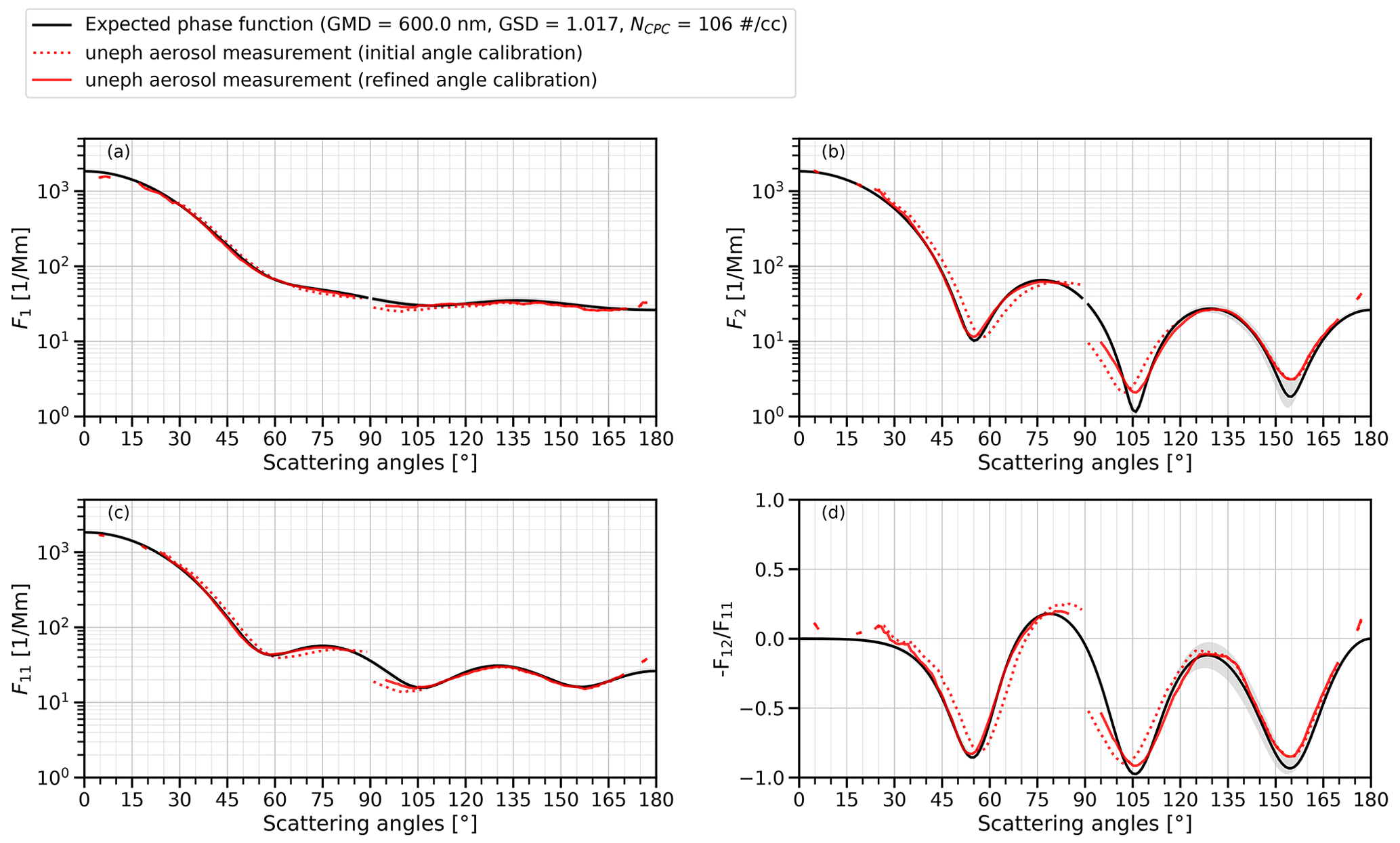
Figure 6 Expected and measured results for a PSL size standard with geometric mean diameter (GMD) of 600 nm for (a) F₁, (b) F₂, (c) F₁₁, and (d) $-F_{\mathrm{12}}/F_{\mathrm{11}}$. The expected curves are based on the Mie theory for homogeneous spheres constrained with a certified mean particle diameter (600 nm), geometric standard deviation (GSD =1.017) inferred from the reported coefficient of variation, and particle number concentration measured by a CPC (N_CPC). The gray shading corresponds to the uncertainty range of the expected phase functions if the certified GMD is perturbed by the reported uncertainty (±9 nm). The uNeph measurement is processed with finally calibrated q values and two different angle calibration curves. The dashed red line represents the initial angle calibration, whereas the solid red line represents the refined angle calibration, based on optimized pinhole center coordinates.

The fact that good agreement is achieved at the end of this optimization process for one specific calibration aerosol does not necessarily imply that the calibration constants are physically meaningful. Therefore, the uNeph measurement still needs to be validated, using aerosol samples with well-constrained properties. Such validation results are presented in Sect. 5.

It can be seen in Fig. 6 that the final calibrated phase function data have a gap in the angle range between ∼ 85^∘ and ∼ 95^∘. The angle of the camera's central axis relative to the laser beams was not optimally chosen in the uNeph prototype, such that the portions of the forward and backward beams corresponding to this angle range fall outside the camera's field of view. This type of angular truncation (side angle truncation) is unfortunate; however, it does not substantially affect the retrieval of aerosol parameters from uNeph measurements, as shown in Moallemi et al. (2022).

4.4 Measurement error assessment

To better understand and quantify the errors in uNeph-measured phase functions, we developed an instrument error model. This model contains the major uNeph error sources and uncertainty values for the parameters that govern each type of error. As demonstrated in Sect. 4.2 and 4.3, uncertainties in the exact laser polarization state and angle calibration are important sources of uNeph measurement error. Air background subtraction and measurement precision also contribute to the measurement error. We account for these four independent sources of error and consider their contributions to the total phase function measurement error (σ_tot) to be independent of each other. Hence, we combine them following standard error propagation for independent errors:

$$\begin{array}{}\text{(4)}& {\mathit{\sigma }}_{\mathrm{tot},l}\left(\mathit{\theta }\right)=\sqrt{{\mathit{\sigma }}_{\mathit{\theta },l}^{\mathrm{2}}\left(\mathit{\theta }\right)+{\mathit{\sigma }}_{\mathrm{BG},l}^{\mathrm{2}}\left(\mathit{\theta }\right)+{\mathit{\sigma }}_{q,l}^{\mathrm{2}}\left(\mathit{\theta }\right)+{\mathit{\sigma }}_{\mathit{\epsilon },l}^{\mathrm{2}}\left(\mathit{\theta }\right)},\end{array}$$

where σ_θ,l, σ_BG,l, σ_q,l, and σ_ε,l represent individual contributions to the phase function error arising from uncertainties in angle calibration, background subtraction, polarization state calibration, and signal precision, respectively. The subscript l is a placeholder denoting the errors of F₁, F₂, F₁₁, or $-F_{\mathrm{12}}/F_{\mathrm{11}}$. A detailed description on the evaluation of different error components is provided in Sect. A5 of Appendix A.

The total measurement error, σ_tot,l, obtained using the error model based on Eq. (4) and its constituting components, is shown in Fig. 7 for the 600 nm PSL aerosol test case. The black lines in Fig. 7e–f demonstrate that the total measurement error strongly depends on the angle, due to variable contributions from individual error components. In this example, the estimated total error remains below 10 % in F₁₁ for most angles and below 0.1 (absolute) in $-F_{\mathrm{12}}/F_{\mathrm{11}}$ for all angles. The complexity of the uNeph measurement errors makes it necessary to use an error model for precise error estimates as a function of phase function shape, aerosol concentration, and scattering angle. The 600 nm PSL aerosol test case, which was used to illustrate how different components contribute to the measurement error, is not a rigid test for the error model, given that these measurement data were also used to refine the angle calibration (Sect. 4.3). Therefore, further validation of the estimated error magnitudes is presented for the uNeph validation experiments discussed in Sect. 5.2.

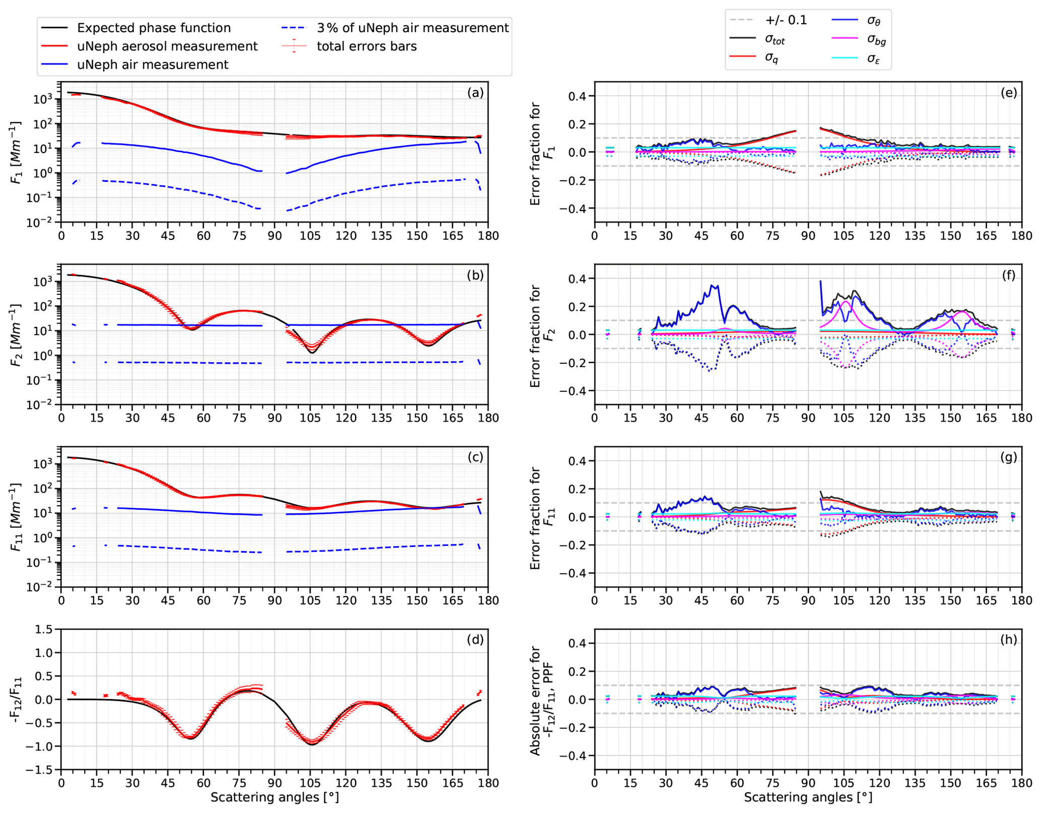
Figure 7 Panels (a), (b), (c), and (d) are the angular light scattering measurements, with total errors for the 600 nm PSL aerosol particles (red lines). The black lines are the expected angular measurements that were calculated using the Mie theory, according to the description in Sect. 4.3. Panels (e), (f), and (g) present the estimated measurement errors in relative terms for F₁, F₂, and F₁₁, respectively. Panel (h) presents the estimated contributions to error of $-F_{\mathrm{12}}/F_{\mathrm{11}}$ in absolute terms. The contribution of air background uncertainty to measurement error remains small (magenta lines in panels on the right), unless the aerosol phase function (red lines in panels on the left) approaches values only slightly above 3 % of the air background (dashed blue lines). This effect is nicely seen in panels (b) and (f) at angles ∼ 105 and ∼ 155^∘.

5 Instrument validation and example application

5.1 Validation of phase function absolute values

The calibration approach for uNeph described in Sect. 4.2 is designed to provide phase matrix elements F₁₁(θ) and F₁₂(θ) in absolute units ([Mm⁻¹ sr⁻¹]), as opposed to just providing normalized phase matrix elements P₁₁(θ) and P₁₂(θ) ([sr⁻¹]). Here, we assess the level of accuracy of the measured absolute values, which depends on the accuracy of the gain calibration factors G_i (Eq. 3) and the precision of the compensated signal ξ. To do so, we used monodisperse PSL size standards with diameters of 240 and 600 nm and the experimental setup shown in Fig. 3b. Validation was done for F₁(θ) and F₂(θ) measured by uNeph. The size distribution parameters (modal size and width) and RI values are fixed and known for PSL aerosols, thus making measured F_i(θ) strictly proportional to the particle number concentration at any angle. Therefore, it is possible, when using the Mie theory, to infer the particle number concentration directly from F_i(θ_j) measured at a single angle θ_j. This was done for all angles with valid uNeph measurements, for the two polarization set points, and for the two PSL sizes. Statistics of the particle number concentration values determined with this approach are provided in Table 1 (fourth and fifth column). The coefficients of variation (CV) of the uNeph-derived particle number concentrations over θ were as low as 4 %, 12 %, 5 %, and 2 % for the two PSL sizes and polarization set points. These results demonstrate that the precision of the gain calibration for single angles is very high, given that errors in PSL size distribution properties and other random noise can also influence the coefficients of variation. The relative bias of the mean uNeph-derived particle number concentrations compared against independent measurements by a CPC is listed in the last column of Table 1. The agreement is excellent, with bias ranging from −4.6 % to +3 %. This is actually much better than the specified CPC uncertainty of ∼ 10 %. Altogether, we conclude that the gain calibration is very precise and that there is no evidence of systematic bias that goes beyond the CPC uncertainty.

Table 1 Validating the absolute values of measured phase functions using PSL size standards and an independent number concentration measurement from a CPC.

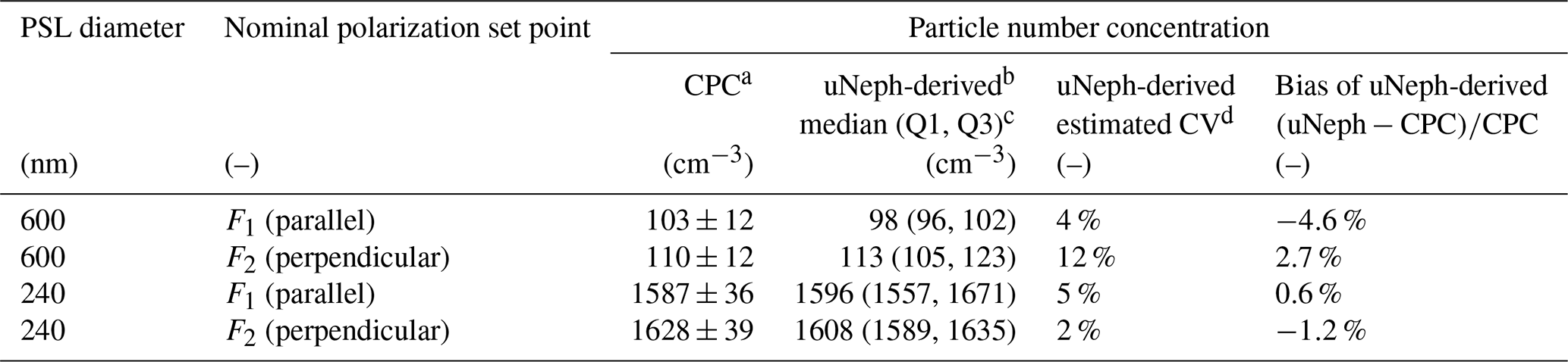
^a The mean CPC measurements with the standard deviation as error values (CPC uncertainty of ∼ ±10 %).
^b This requires the Mie theory to be constrained with the reported diameter and CV of the PSL size standards. The number concentration was independently derived from the data points at each angle. Here we report the statistics of the results from all measured angles.
^c Q1 and Q3 refer to the lower and upper quartiles, respectively.
^d The coefficient of variation is estimated using the formula (0.741× interquartile range)$/$median, which is insensitive to outliers.

5.2 Validation of phase functions using quasi-monodisperse aerosol

The uNeph data presented in Fig. 7 do not validate the instrument performance for measuring any type of phase function because this experiment was also used to refine the angle calibration. Therefore, uNeph performance was further validated by probing quasi-monodisperse spherical aerosol particles with known complex RI and diameters of 200, 400, 600, and 800 nm. These validation aerosols were generated by extracting a narrow size cut from a broad unimodal DEHS aerosol by means of an AAC (see Fig. 3b for the experimental setup). The sampling period was ∼ 60 min for each size and included the recording of multiple repeats of data at different exposure times (0.1 s $\le t_{\mathrm{expo}}\le$ 100 s) to ensure that valid signals were collected for all angles and polarization set points (Sect. 3.2.1). The aerosol number concentration was quite stable, and small drifts during the experiments were accounted for in the data analysis.

DEHS is a liquid, which therefore results in spherical particles when aerosolized. This makes it possible to use the Mie theory to calculate the expected light scattering phase functions. Nevertheless, the true phase function is not exactly known, due to uncertainties in the aerosol parameters that are required for input in the Mie calculation. A complex RI of 1.455+0i at 532 nm was used, based on Pettersson et al. (2004). The AAC-classified particles were assumed to have lognormal size distributions, with the best estimates for the modal diameter inferred from AAC aerodynamic diameter set points (see Table S3) and for the number concentration taken from the CPC measurement. To account for uncertainties in the properties of the AAC-extracted aerosol, a Monte Carlo simulation was performed to calculate a range of expected phase functions by varying the size distribution parameters. The complex RI was held at a fixed value, and normally distributed errors were assumed for modal diameter and number concentration, with coefficients of variation equal to 3 % and 10 %, respectively. The width of the lognormal size distribution, expressed as a geometric standard deviation (GSD), is not exactly known. Therefore, possible GSD values were assumed to be evenly distributed between the limits 1.04 and 1.08. F₁₁ and $-F_{\mathrm{12}}/F_{\mathrm{11}}$ were calculated for 1000 sets of randomly drawn size distribution parameters as described above, and the interquartile range of all resulting phase function values at a given angle is assumed to represent uncertainty in the true phase function as constrained by AAC and CPC.

The uNeph validation results are presented in Fig. 8. The uncertainty range of the expected F₁₁ and $-F_{\mathrm{12}}/F_{\mathrm{11}}$ is shown as gray shading, and the measured phase functions are shown as red lines, with the error bars calculated with the error model presented in Sect. 4.4. The F₁₁ measurements fall well within the uncertainty range of expected phase functions over all available angles and for all four sizes (top panels). More precisely, most of the data points fall into the uncertainty range of the predictions, even without an error allowance on the uNeph measurement. There is hardly any disagreement between the expected and measured F₁₁ that exceeds the measurement errors. The findings are quite equivalent for the $-F_{\mathrm{12}}/F_{\mathrm{11}}$ function; the measurements fall well within the uncertainty range of the expected phase functions (bottom panels in Fig. 8) for the most part, even without allowing for measurement error. The disagreement that exceeds the estimated measurement errors only occurs at a few angles for the 800 nm particles. The uncertainties in the true phase functions, i.e., the width of the gray shading, are quite considerable, despite using well-defined reference aerosols. This impedes a stringent test of the error model, i.e., reliable identification of potentially underestimated measurement errors.

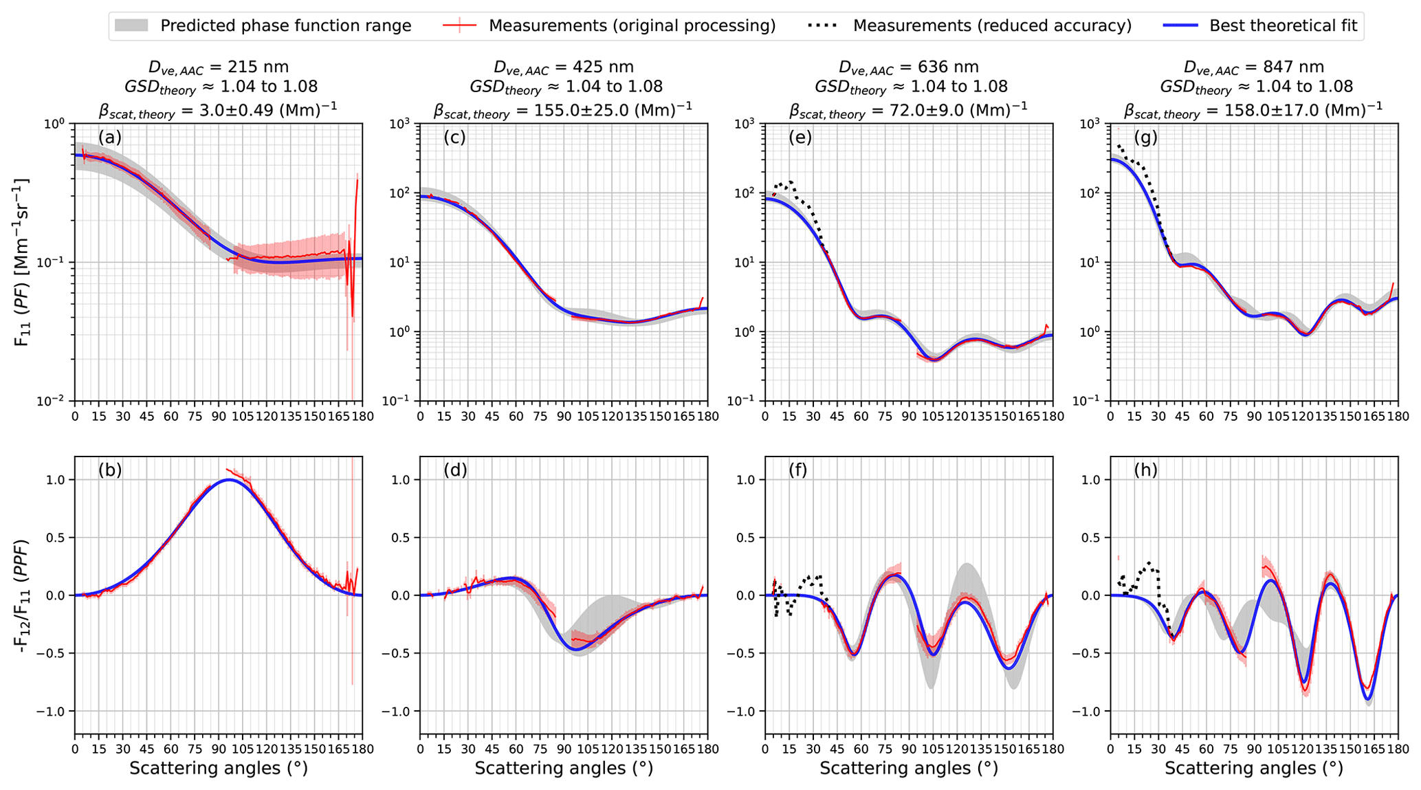
Figure 8 Phase function (F₁₁) and polarized phase function $(-F_{\mathrm{12}}/F_{\mathrm{11}})$ measurements for different monodisperse DEHS aerosol test cases. The nominal aerodynamic diameters are 200 nm (a, b), 400 nm (c, d), 600 nm (e, f), and 800 nm (g, h), and the respective particle number concentrations measured by a CPC were 190±8, 494±11, 59±4, and 70±5 cm⁻³. The volume equivalent diameter, D_ve, for each sample is reported in the column headings. The gray shading indicates the uncertainty range of the independently constrained phase functions, considering the uncertainties in the input parameters for the Mie calculations (see Sect. 5.2 for details). The blue lines in the figure are the best-fit phase functions obtained with a least squares minimization of the residuals of the calculated Mie curves compared with the measurement.

An alternative approach to validating the phase function measurements is to use them to retrieve the properties of the test aerosol size distributions, which are assumed to be of a lognormal shape and are described by the vector ν_PSD defined in Eq. (5a), with the elements of the geometric mean diameter (d_m), geometric standard deviation (GSD), and total particle number concentration (N_tot).

$$\begin{array}{}\text{(5a)}& {\mathit{\nu }}_{\mathrm{PSD}}=\left[\begin{array}{c}{d}_{\mathrm{m}}\\ \text{GSD}\\ N_{\mathrm{tot}}\end{array}\right]\end{array}$$

For this purpose, a simple retrieval scheme was applied to retrieve ν_PSD, optimized such that the corresponding phase functions calculated with the Mie theory achieve the best fit with the phase function measurement data, specifically F₁ and F₂, according to the least squares minimization given in Eq. (5b).

$$\begin{array}{}\text{(5b)}& \begin{array}{rl}& {\mathit{\nu }}_{\mathrm{PSD},\mathrm{fit}}=\underset{{\mathit{\nu }}_{\mathrm{PSD}}}{min}\\ & \left({\displaystyle \frac{\begin{array}{c}{\sum }_{{\mathit{\theta }}_{\mathrm{1}}}^{{\mathit{\theta }}_N}{\left(\ln \left(F_{\mathrm{1},\mathrm{meas}}\right({\mathit{\theta }}_i\left)\right)-\ln \left(F_{\mathrm{1},\mathrm{Mie}}\left({\mathit{\theta }}_i,{\mathit{\nu }}_{\mathrm{PSD}}\right)\right)\right)}^{\mathrm{2}}\\ +{\sum }_{{\mathit{\theta }}_{\mathrm{1}}}^{{\mathit{\theta }}_N}(\ln \left(F_{\mathrm{2},\mathrm{meas}}\left({\mathit{\theta }}_i\right)\right)-\ln \left(F_{\mathrm{2},\mathrm{Mie}}\left({\mathit{\theta }}_i,{\mathit{\nu }}_{\mathrm{PSD}}\right)\right){)}^{\mathrm{2}}\end{array}}{N}}\right),\end{array}\end{array}$$

where N is the number of measured angles. The complex refractive index of DEHS at 532 nm was again taken as 1.455+0i (Pettersson et al., 2004). The blue lines in Fig. 8 correspond to F₁₁ and $-F_{\mathrm{12}}/F_{\mathrm{11}}$ being calculated with the best fit of ν_PSD. These curves match the measurement data within measurement error, except for very few data points. This shows that the shape of the measured phase functions is physically meaningful. The corresponding retrieved size distribution parameters are included in Table S3, along with independent data. The retrieved GSD values ranged from 1.035 to 1.065, which is very narrow but within a plausible range for the given AAC-resolution parameter settings. The retrieved number concentrations agree with the CPC data to within −2 % to +6 %, which falls within the uncertainty range of the CPC. The retrieved diameters agree with the AAC data to within −0.5 % to −3.8 %, which is a very good agreement, though located at the edge of expected AAC uncertainty. The fitted theoretical F₁₁ (blue lines) also fall within the uncertainty range of the true phase functions, as indicated by the gray shading. However, the course of the blue lines within the gray shaded areas is not random; instead, they closely follow one edge of the shading for the three AAC set points shown in Fig. 8c to h. Additional analyses, presented in Fig. S21, demonstrate that the measured phase functions are self-consistent across different angles. This suggests that the small but systematic low bias of the retrieved diameters compared to AAC set points could just as plausibly be attributed to a small bias of the AAC.

These results demonstrate the successful validation of uNeph. The magnitude of the modeled uNeph measurement errors is plausible, although drawing firm conclusions is difficult because the uncertainties in the properties of the validation aerosol translate to considerable uncertainties in the predicted phase functions. In other words, the information content of the phase functions measured by uNeph for a unimodal aerosol with known RI is so high that the aerosol properties (i.e., d_m, GSD, and N_tot) retrieved with a suitable inversion algorithm have uncertainties that are similar to or even smaller than the prior knowledge of these properties. This statement is in line with the findings of the uNeph information content analysis presented in Moallemi et al. (2022).

The uNeph measurement accuracy appears to be comparable to that of previous laser-imaging-type nephelometers. Dolgos and Martins (2014) estimated the errors to be on the level of ∼ 5 % for F₁₁ and ∼ 0.05 (absolute) for PPF in their laser imaging nephelometer. Ahern et al. (2022) reported a precision of ±2 % for F₁₁(θ) and a positive bias of ∼ 30 % for the integrated scattering coefficient obtained by integrating F₁₁(θ) over θ.

The results for the 200 and 400 nm examples shown in Fig. 8 (left panels) show that uNeph can provide phase function measurements between 5 and 175^∘ under favorable conditions. On the other hand, a portion of the phase functions measured for the 600 and 800 nm cases in the ∼ sub 35^∘ angular range was discarded during the data processing step described in Sect. 3.2.1. This is the consequence of operating uNeph in an overly sensitive configuration combined with insufficient dynamic range, which potentially leads to systematic measurement bias when probing large aerosol particles (see Sect. 3.2.1 for an extensive discussion). Unfortunately, the CCD was accidentally operated without cooling, which affected its dynamic range compared to operation in a cooled state. To investigate how relaxing criteria for filtering proper signals can affect the measurement results, we modified the data processing code to retain the image data acquired with t_expo=0.1 s. These data, shown as dashed black lines in Fig. 8, are systematically larger than the predicted values. Therefore, it is considered important to rigorously filter the raw data, following the procedure described in Sect. 3.2.1, to achieve high-quality data.

5.3 uNeph–GRASP retrieval of aerosol properties

Retrieving aerosol properties from measured phase functions is a central application of aerosol polarimetry. Here we present a first test experiment to demonstrate feasibility of aerosol property retrieval from uNeph measurements. We used the GRASP algorithm (Dubovik et al., 2014) to solve the inverse problem. GRASP is a versatile and well-established inversion algorithm used in a wide range of aerosol remote sensing applications (Dubovik et al., 2021). GRASP uses a multiterm least squares minimization in measurement space as the basis for solving the aerosol–light scattering inverse problem, including the consideration of a priori constraints. It allows for using multiple types of measurement inputs and retrieving different types of aerosol properties. For our purpose, we tailored the open-source version, GRASP OPEN (https://www.grasp-open.com/; last access: 25 May 2022), to handle the single-scattering inverse problem for the uNeph phase function data, hereafter referred to as the uNeph–GRASP inversion.

GRASP is mainly designed for atmospheric applications with relatively wide size distributions. The standard GRASP kernel is a precomputed lookup table with a finite resolution on a diameter scale. This can result in discretization errors during the retrieval for lognormal size distributions with a GSD smaller than around 1.2, while such errors are negligible for wider size distributions. Therefore, to assess the uNeph–GRASP inversion (i.e., to investigate the retrieval of the aerosol volume size distribution and RI from uNeph-measured F₁₁ and $-F_{\mathrm{12}}/F_{\mathrm{11}}$), a sufficiently broad aerosol size distribution had to be generated. For this purpose, we generated a broad unimodal DEHS aerosol, following the experimental procedure illustrated in Fig. 3c and explained in Sect. 2.2.

The aerosol was first generated and collected in a tank serving as the holding chamber. Then the aerosol was sampled from this tank and probed by uNeph in addition to an SMPS and CPC to provide independent measurements of the particle size distributions and number concentrations, respectively. Sampling from the tank led to the gradual dilution and concurrent decrease in the aerosol concentration during the uNeph measurement. In order to minimize the systematic measurement bias, this concentration drift was accounted for in the uNeph data processing. Specifically, the time-resolved particle number concentration data measured by the CPC were used to compensate for the F₁(θ) and F₂(θ) data, which were measured by uNeph at different times (∼ 5 min total measurement time per polarization set point, with a 1 h time gap in between).

The measurement space considered in the uNeph–GRASP inversion consists of either (i) F₁₁ only or (ii) F₁₁ and $-F_{\mathrm{12}}/F_{\mathrm{11}}$. The DEHS test aerosol consists of an ensemble of homogeneous spherical particles, with equal RI and a unimodal size distribution. Therefore, we chose the following two variants of the aerosol state space representations for the uNeph–GRASP inversion: (i) the lognormal volume size distribution representation (state parameters include total volume concentration, V_tot, geometric mean radius, r_g, and geometric standard deviation, GSD) or (ii) the binned size distribution representation (state parameters include volume concentrations at each size bin, $V_k=\mathrm{d}V/\mathrm{d}\log r\left(r_k\right)$, for 22 size bins, with central radii fixed at positions r_k). For both variants, the GRASP default size range covering particle radii from 0.05 to 15 µm was used, and particles were assumed to be spherical, with real and imaginary parts of RI being allowed to vary in the ranges from 1.35 to 1.7 and 10⁻⁵i to 0.2i, respectively. The GSD was allowed to vary across the full available range, from 1.2 to 3, for the lognormal size distribution representation. The parameters for imposing size distribution smoothness constraints for the binned size distribution representation were chosen, based on the values used by Dubovik et al. (2011), for an aerosol property retrieval over a single satellite pixel (difference order of 3 and Lagrange multiplier of 0.005 for the volume size distribution). No further constraints, such as forcing the size distribution tails to 0, were applied.

Figure 9 presents the F₁₁ and −F₁₂/F₁₁ measured by uNeph for the test sample, together with the fit results for different uNeph–GRASP inversions (fit refers to F₁₁ and −F₁₂/F₁₁ calculated using the GRASP forward model and the inverted aerosol properties). All four uNeph–GRASP inversion configurations result in largely identical fit curves (blue and red colored lines in Fig. 9a and b), apart from the exception in the angle range ∼ 150 to 170^∘ for the binned configurations, which will be addressed later in this section. The GRASP fits to F₁₁ match the measurements at the majority of angles (Fig. 9a). Discrepancies slightly beyond error margins only occur in the angle ranges from ∼ 95 to ∼ 105^∘ (all retrieval settings) and from ∼ 155 to ∼ 170^∘ (lognormal retrieval settings). The GRASP fits to the $-F_{\mathrm{12}}/F_{\mathrm{11}}$ function match the uNeph measurements reasonably well (Fig. 9b). However, noticeable differences beyond the error margins occur in the angle ranges from ∼ 60 to ∼ 85^∘ and from ∼ 110 to ∼ 160^∘. The exact reasons for these discrepancies for F₁₁ and $-F_{\mathrm{12}}/F_{\mathrm{11}}$ remain elusive, as multiple factors can play a role, including the residual bias in the compensated aerosol concentration drifts, slightly underestimated measurement errors, or fine structures in the true aerosol size distribution shape that cannot be reproduced by the aerosol size distribution representations implemented in GRASP.

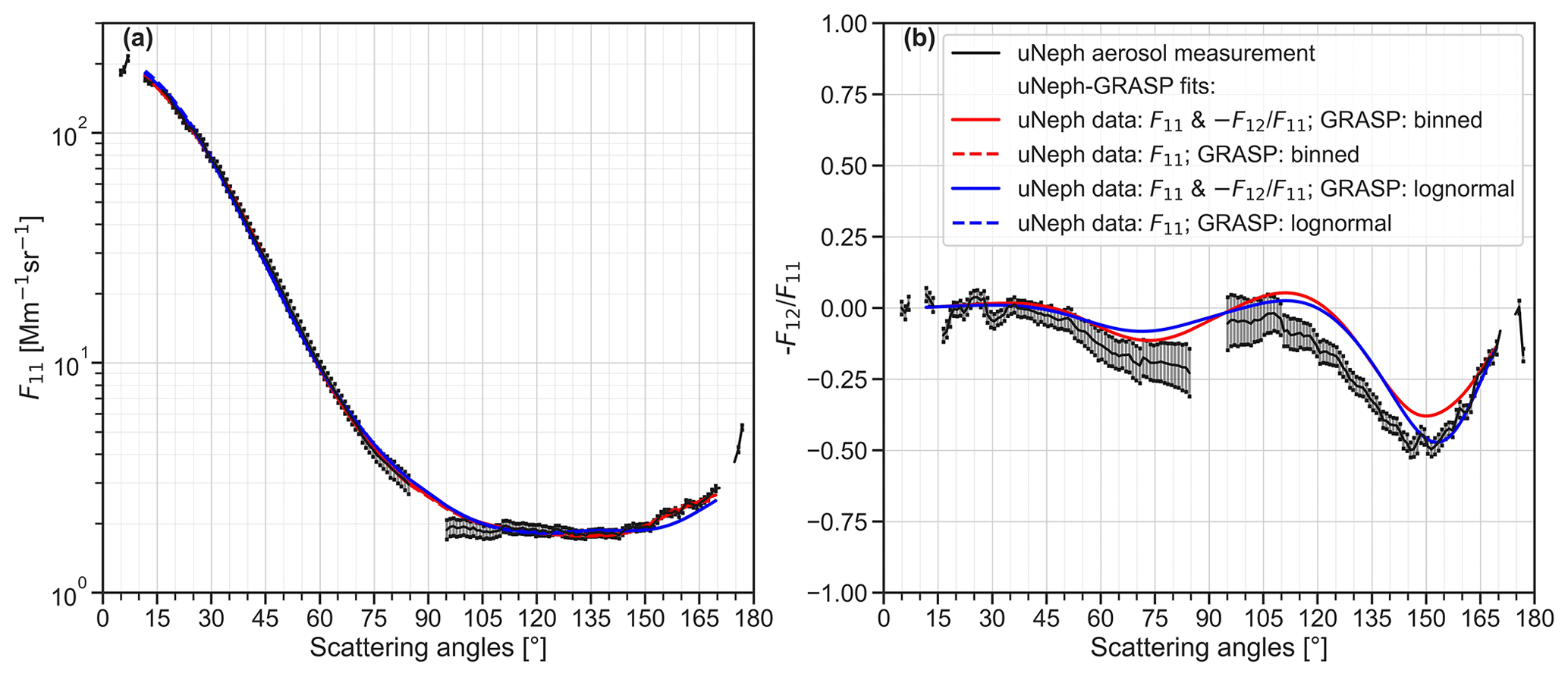
Figure 9 Phase function (F₁₁) and polarized phase function $(-F_{\mathrm{12}}/F_{\mathrm{11}})$ measurements by the uNeph and GRASP retrieval results for the broad unimodal DEHS test case.

The uNeph–GRASP inversion results for the unimodal DEHS aerosol (i.e., retrieved aerosol volume size distribution and complex RI) are shown in Fig. 10. The volume particle size distributions (VPSDs) retrieved with the four uNeph–GRASP inversion variants are in close agreement with each other (red and blue colored lines in Fig. 10a), which explains the close match of the four corresponding GRASP fits to F₁₁ and $-F_{\mathrm{12}}/F_{\mathrm{11}}$ in Fig. 9. There is a small but clearly discernible difference in the retrieved VPSDs from the binned inversions, which have additional minor modes to the right of the main mode. This leads to better agreement between the GRASP fit and the measured F₁₁ in the angle range of 150–170^∘ (Fig. 9a), compared to the other retrievals. However, substantial particle volume in this size range is not expected, based on the aerosol generation process; hence, it could be a result of an overfitting measurement bias. The uNeph–GRASP inversion also retrieves both the real and imaginary parts of the RI. These are in very close agreement among the four inversion variants; i.e., maximal absolute differences are as small as 0.018 and ∼ $\mathrm{3}\times {\mathrm{10}}^{-\mathrm{4}}i$ for the real and imaginary parts, respectively (colored markers in Fig. 10b).

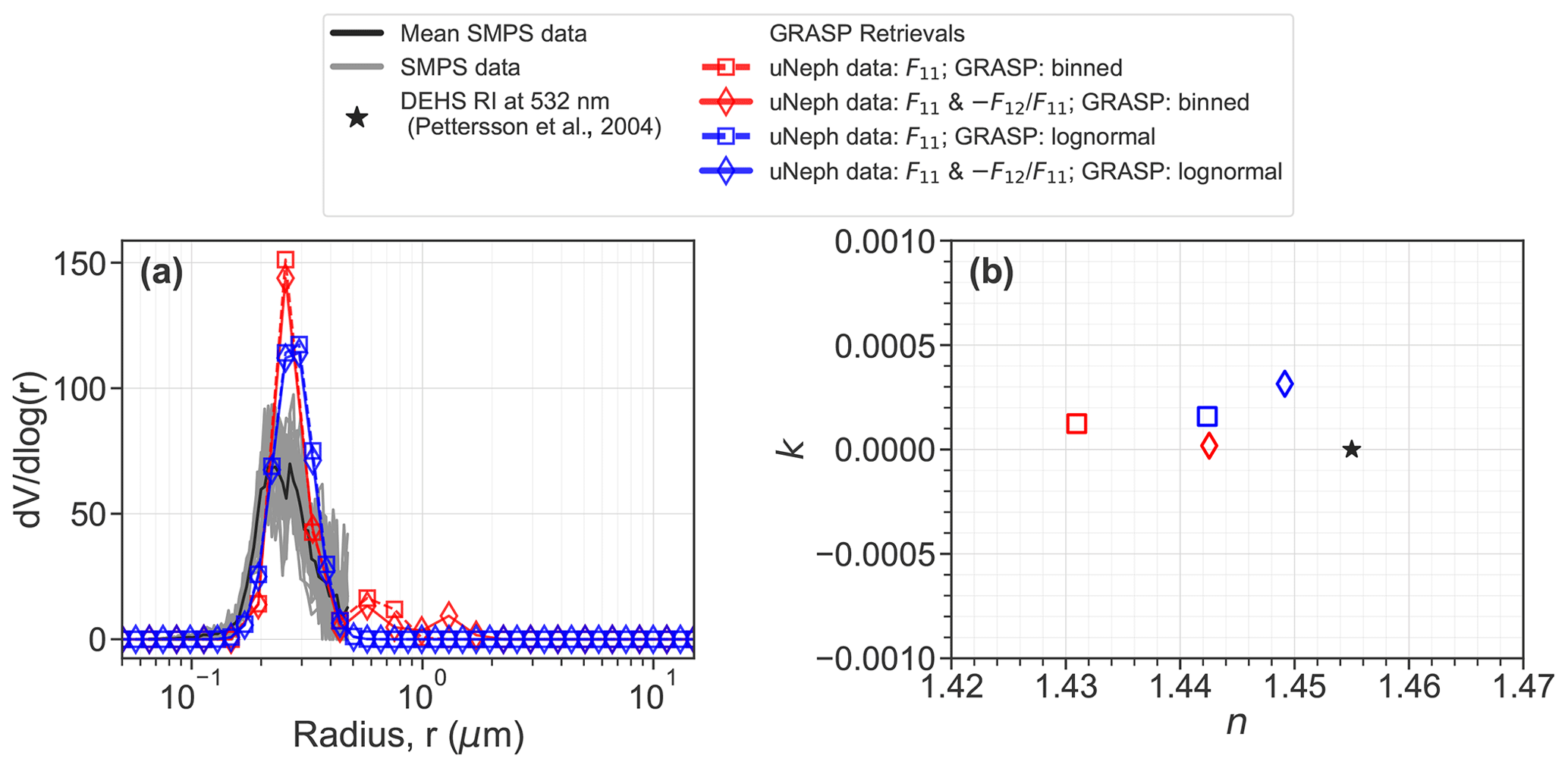
Figure 10 Retrieval results obtained by applying GRASP to the uNeph data (a) volume size distribution compared against independent SMPS measurements. (b) Real (n) and imaginary (k) parts of the complex refractive index (RI) compared against the literature data.

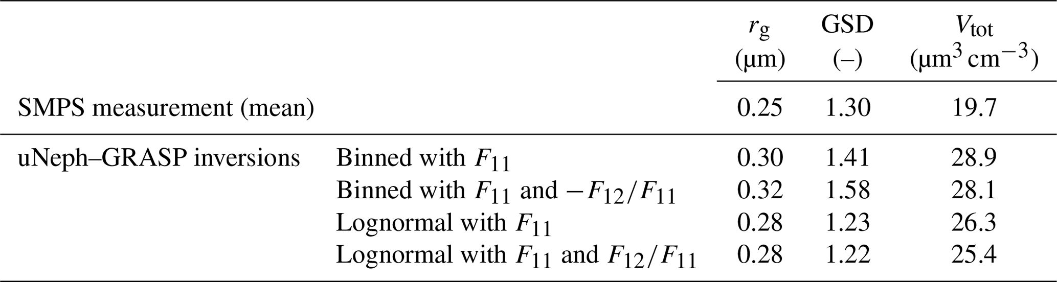
The results discussed so far show that the uNeph–GRASP inversion is robust in the sense that it leads to essentially identical retrieval results for different inversion variants applied to the unimodal test aerosol, which also reproduce the measured F₁₁ and $-F_{\mathrm{12}}/F_{\mathrm{11}}$ reasonably well. As a last step, we compare the retrieval results with independently known or measured properties of the aerosol sample. Validation of retrieved VPSD is done against independent measurements by an SMPS. Figure 10a shows that the mode and width of the size distributions from SMPS (black line) and the uNeph–GRASP inversions (colored lines) are consistent, while the magnitude of the retrieved size distribution is larger than that of the independent measurement. For a quantitative comparison, the integral properties' total volume concentration (V_tot), geometric mean radius (r_g), and GSD were calculated from the measured and retrieved VPSDs (when not directly delivered as retrieved parameter).

The results listed in Table 2 demonstrate the agreement for V_tot between SMPS and each retrieval result as being within 45 % or better. This is a fair agreement, though it is outside the range of expected uncertainties in either approach under optimal performance. The reasons for this discrepancy remain elusive. In contrast to V_tot, the retrieval results for the state parameters r_g and GSD indicate that the uNeph–GRASP retrieval and the SMPS measurement agree quite well (Table 2). The binned retrievals have the largest r_g and GSD, which is caused by the minor tail in the retrieved VPSD at larger diameters. Agreement with the SMPS remains good despite this retrieval artifact. The lognormal retrieval variants provide slightly larger r_g than the SMPS (+10 %; 0.275 µm instead of 0.250 µm) and slightly narrower GSD (∼ 1.22 instead of 1.3). This is a good agreement, thus validating the uNeph–GRASP inversion for retrieving the VPSD width and size for unimodal aerosols.

Table 2 Size distribution parameters (geometric mean radius, r_g; geometric standard deviation, GSD; and total volume concentration, V_tot) of the broad aerosol test case obtained from SMPS measurements and retrieved from uNeph–GRASP inversions.

Excellent agreement between independent knowledge and uNeph–GRASP inversion was also achieved for the RI. The literature value for n (i.e., the real part of the RI) of DEHS (1.455; Pettersson et al., 2004) is virtually identical to the retrieval results (∼ 1.431 to 1.449), whereby the lowest retrieval value originates from the F₁₁-only or binned retrieval, which has a second mode in the size distribution. The retrievals also correctly return a negligibly small value for k, i.e., the imaginary part of RI ($\mathrm{1}\times {\mathrm{10}}^{-\mathrm{5}}i$ to $\mathrm{5}\times {\mathrm{10}}^{-\mathrm{4}}i$), which is perfectly consistent with the fact that DEHS is a non-absorbing liquid, with k smaller than $\mathrm{1}\times {\mathrm{10}}^{-\mathrm{4}}i$ (Verhaege et al., 2009).

The accuracy achieved in retrieving aerosol properties for the broad unimodal DEHS aerosol test case can be explained by the high information content of uNeph measurements. Recently, an information content analysis conducted by Moallemi et al. (2022) demonstrated that for unimodal DEHS aerosol test cases, even a polar nephelometer with high angular resolution and basic radiometric configuration, i.e., with only F₁₁ measurements at a single wavelength, can be quite informative with respect to retrieving aerosol state parameters. Considering that the level of the uNeph measurement errors for the broad unimodal test aerosol is similar to or lower than the base case in the aforementioned information content study, it is not surprising that aerosol properties can be retrieved with high accuracy. Furthermore, the missing benefit from the retrieval accuracy of including $-F_{\mathrm{12}}/F_{\mathrm{11}}$ is not surprising, as this benefit becomes more prominent for more complex aerosols, as shown by Moallemi et al. (2022).

It should be noted that retrieval of k using light scattering measurements is generally more challenging than for other aerosol properties. Often, accurate absorption retrievals require auxiliary measurements, such as aerosol extinction or absorption (Schuster et al., 2019). The information content study by Moallemi et al. (2022) indicates that the scattering measurement has a higher information content for the retrieval of k when the aerosol is non-absorbing. This, in combination with limited complexity of the probed aerosol, explains why good results were also achieved by the uNeph–GRASP inversion for the retrieval of k for the non-absorbing DEHS aerosol test case.

Overall, the results from this experiment validate the uNeph–GRASP inversion to perform in situ polarimetric measurements and retrieve aerosol properties. Espinosa et al. (2017, 2019) have already shown the applicability of GRASP for aerosol property retrieval from laser imaging nephelometer measurements. Our results demonstrate that the GRASP inversion can also be applied to measurements from more compact single-wavelength laser imaging nephelometers, such as uNeph.

6 Conclusions

This paper introduces a new laser imaging nephelometer, uNeph, which measures the scattering coefficient as a function of polar angle at two different states of polarization. These measurements are used to derive the absolute scattering phase function, F₁₁, and polarized phase function, $-F_{\mathrm{12}}/F_{\mathrm{11}}$. The instrument design and all key data processing steps are presented. We further discuss all calibration parameters and the calibration process relying on measuring both gases and a PSL aerosol size standard to achieve optimal calibration accuracy.

We constructed an error model and characterized the uncertainties in the parameters driving the overall measurement error. This makes it possible to provide quantitative estimates of measurement error, which depend on actual results such as phase function shape and absolute scattering intensities. Estimated measurement errors are mostly between 5 % and 10 % for F₁₁ and smaller than ∼ 0.1 (absolute) for $-F_{\mathrm{12}}/F_{\mathrm{11}}$, while errors can become larger close to the lower limit of detection.

The uNeph instrument was validated using DEHS monodisperse aerosol particles with aerodynamic diameters of 200, 400, 600, and 800 serving as reference. Good agreement was achieved between the measurements and theoretical phase functions predicted for the reference aerosols. The error model provides plausible measurement errors. However, it was not possible to rigorously validate the error model. This is mainly due to the fact that the estimated measurement errors translate to corresponding uncertainties in the aerosol property space which are smaller than or comparable to the available independent knowledge of the reference aerosol properties. The results further demonstrate that it is possible to cover an angle range between ∼ 5 and ∼ 175^∘ for suitable samples. The small detection cell combined with high sensitivity imposes some limitations. For instance, a smaller sensitive volume is more susceptible to statistical fluctuations in the average particle number inside the sensitive volume, which can limit temporal resolution at low particle number concentrations. Moreover, signal saturation can limit the maximum detectable particle size, above which the systematic bias occurs in parts of the phase function, if operated at comparable sensitivity for homogeneous samples (e.g., particle-free air).

Finally, we performed an experiment to test the combination of the uNeph and the GRASP inversion algorithm for aerosol property retrievals. This was successfully achieved for a broad unimodal DEHS aerosol sample; i.e., retrieved volume concentration, modal size, size distribution width, and complex refractive index agreed within the uncertainty level with independent measurements and the literature data. Generally, these experiments demonstrate the high information content of uNeph measurement data; i.e., radiometric calibration and measurement errors are sufficient for quantitative aerosol retrieval.

Overall, uNeph was successfully validated, and our results show the applicability of a downsized laser imaging nephelometer. Downsizing the instrument posed challenges, which result in slower measurements of aerosol samples containing large particles present in small numbers. At the same time, the dimensions of uNeph have been considerably reduced compared to previous laser imaging nephelometers. This demonstrates that the operation of such instruments on, e.g., unmanned aerial vehicles is achievable. Such increased flexibility enables the acquisition of in situ aerosol polarimetry data sets, which can greatly benefit the remote sensing community for validating and improving existing retrieval algorithms. Future improvements to uNeph will aim at increasing the dynamic range and the number of measurement wavelengths, with the goal to use it in laboratory and field settings for aerosol characterization, in addition to the validation and optimization of polarimetric aerosol property retrievals for more complex aerosols.

Appendix A: Image data reduction

A1 Hot-pixel removal

To remove hot pixels, we used the median of multiple dark image samples (three repeats) that were acquired at an exposure time of 700 s, which is denoted as ${\stackrel{\mathrm{‾}}{\text{Im}}}_{D,\mathrm{700}\mathrm{s}}$. Assuming that the dark current is mostly homogeneous over the image pixels of ${\stackrel{\mathrm{‾}}{\text{Im}}}_{D,\mathrm{700}\mathrm{s}}$, we calculated the median and standard deviation (SD) of all the pixel values of ${\stackrel{\mathrm{‾}}{\text{Im}}}_{D,\mathrm{700}\mathrm{s}}$, which were used in Eq. (A1) to define a hot-pixel signal threshold (L_hot).

$$\begin{array}{}\text{(A1)}& L_{\mathrm{hot}}=\text{median}\left({\stackrel{\mathrm{‾}}{\text{Im}}}_{D,\mathrm{700}\mathrm{s}}\right)+\mathrm{1.5}\times \text{SD}\left({\stackrel{\mathrm{‾}}{\text{Im}}}_{D,\mathrm{700}\mathrm{s}}\right)\end{array}$$

Any pixel in ${\stackrel{\mathrm{‾}}{\text{Im}}}_{D,\mathrm{700}\mathrm{s}}$ with a signal larger than the threshold value is considered to be a hot pixel and is removed from the image prior to any further signal processing steps. Figure S3 shows the hot pixels in a sample dark image. It should be noted that this process was also tested with dark image samples acquired at exposure times of 215 and 464 s, and the detected pixels were quite similar to the hot pixels obtained by sample images with an exposure time of 700 s. Specifically, the 215 and 462 s test cases detected 2 and 1 hot pixels fewer than the 700 s samples, respectively.

A2 Dark signal characterization

The CCD image data contain a dark signal contribution which also occurs in the absence of any illumination. The dark signal (DS) has two systematic components, namely a constant positive bias (B) and dark current proportional to the exposure time. These can be described with a linear equation, as follows:

$$\begin{array}{}\text{(A2)}& \text{DS}=G_{\mathrm{DC}}\times t_{\mathrm{expo}}+B,\end{array}$$

where G_DC is the proportionality constant for the dark current part. The dark signal also contains superimposed random noise, which is not captured by Eq. (A2). In our analysis, we used two different t_expo values of 4.64 and 700 s to characterize the DS. The DS may vary between pixels. Accordingly, the two constants can be determined either for each pixel or for each angle (after integration over beam cross section). We considered the signal from dark images collected at the short t_expo of 4.64 s (30 sample images) to mainly consist of B. Therefore, the mean values of dark images at t_expo of 4.64 s were used to calculate B. Subsequently, we used the mean signal of dark sample images acquired at the long t_expo of 700 s to obtain G_DC.

To determine the robustness of the dark signal estimation, we applied the dark signal correction on a series of dark image signals acquired over t_expo ranging from 0.1 to 464 s. Residuals of the dark signal compensation, that is, the difference between estimated dark signal and actual dark image signals, were integrated over scatter signal bounds for measured scattering angles (Sect. 3.1.3) and are shown over different t_expo values in Fig. S4. The results show that the dark residual signals, Ξ_DRS(θ), are ∼ ±200 a.u. for the uncooled CCD case over the scattering angles for the sample acquired at t_expo below 215 s, while for the dark image sample at t_expo=464 s, $\left|{\mathrm{\Xi }}_{\mathrm{DRS}}\right(\mathit{\theta }\left)\right|$ values as large as 500 a.u. were also observed. The results further suggest that for the CCD cooled case, the Ξ_DRS(θ) values are ∼ ±200 a.u. for all the tested exposure times. Valid light scattering data near the lower limit of detection can only be achieved if the interference of dark signal residuals is small (i.e., if the contribution of light scattering to the CCD signal substantially exceeds the dark signal residuals). The uNeph data presented in this work were all acquired with uncooled CCD.

A3 Scattering angle calibration procedure

The relationship between the scattering angle and image pixels is determined through the scattering angle calibration. To conduct the scattering angle calibration, a multistepper motor mechanism, which is referred to as the three-dimensional (3D) position probe, was employed. Figure S5a shows the 3D position probe, which is made up of three orthogonal step motors traversing stages which are intended to travel along the xyz coordinate axes, according to the coordinate system depicted in Fig. S5a. A probing arm with a pinhead at the end of the arm was mounted on the traversing stage that travels along the x axis. The function of the 3D positional probe is to probe the spatial location of the optical objective pinhole and different locations along the path of the forward and backward beams. The stepper motors used in the 3D positional probe traverse a distance of 0.025 mm per step.

To conduct the scattering angle calibration, the top cap of the scattering chamber is removed. The 3D positional probe is then mounted on top of the uNeph instrument, such that the probe arm has access to the scattering chamber. The initial step for conducting the angular calibration is the identification of the objective pinhole coordinate. To do so, the probe was moved from a reference position (the origin coordinate) and was carefully displaced with step motor movements until the probe pinhead reached the location of the objective pinhole, which we define as point P. The steps taken by the motors from the origin point were recorded, and based on that, the coordinates of the objective pinhole are specified relative to the origin point. Subsequently, a similar approach is employed to obtain the coordinates of the center of the laser beams in the y–z plane. The next step in the calibration process involves placing the probe pinhead at different locations along the laser beam central axis and within the field of view of the objective pinhole lens. The coordinate of a point along the laser beam center axis is denoted as point S. The polar scattering angle then becomes the following:

$$\begin{array}{}\text{(A3)}& \mathit{\theta }=\arccos \left({\displaystyle \frac{\mathit{S}\mathit{P}\times \widehat{i}}{∥\mathit{S}\mathit{P}∥}}\right).\end{array}$$

In Eq. (A3), P is the objective pinhole position, ν_SP is the vector connecting point S to P with vector length of ∥SP, and $\widehat{i}$ is the unit vector along the x axis (laser beam axis). Figure S5b shows an example scheme where scattering angle geometry is depicted for a case where the probe pinhead is placed at a given location S. When the probe pinhead is located at a given position (e.g., point S), the light reflected off the pinhead will be detected by the imaging unit and generate a bright spot in a sample image captured by the CCD camera. During the calibration process, the probe was placed in 27 different locations along the laser beam center axis of each beam (forward and backward beams). Once placed at each of these locations, a picture of the probe pinhead was taken at the reflected spot. Figure S6a shows an example of the pinhead spot detected by the CCD at a single location, and Fig. S6b shows a composite image of the combination of multiple pinhead spot images that were taken during the scattering angle calibration process. Up to this point, this process has provided pairs of polar angles (Eq. A3) and spots on the CCD image with finite width. As a last step, an exact coordinate on the CCD image (i.e., single representative pixel) is assigned to each of these spots by calculating its center of mass (red dots in Fig. S6).

While the pixel angle information provided by the angular calibration is useful, it is quite limited, and the angular difference (Δθ) between most of the adjacent calibration pixels is larger than 1^∘. Therefore, further processing is required to obtain pixel angle information with an angular resolution of 1^∘. To refine the pixel angle data, the angular calibration points at each of the beam segments (forward or backward) were used to generate a second-degree polynomial fit, which takes angles as input and returns pixel coordinates. These fits can be used to generate a list of refined coordinates corresponding to scattering angles ranging from 3–90^∘ (forward beam) to 90–177^∘ (backward beam), with an angular resolution of 1^∘.

A4 Image transformation and signal integration limits

Sections 3.1.2 and A3 described how to obtain the red fit curve in Fig. 2b, which is a parametrization of pixel coordinates as a function of θ along the centerline of the beam on the CCD image. The next goal is to extract a pixel array representing laser beam image cross sections for each polar angle (θ_i). For this purpose, lines perpendicular to this fit were obtained as follows:

$$\begin{array}{}\text{(A4)}& y-y_{\mathrm{CL}}\left({\mathit{\theta }}_i\right)=-{\displaystyle \frac{\mathrm{1}}{m\left({\mathit{\theta }}_i\right)}}\left(x-x_{\mathrm{CL}}\left({\mathit{\theta }}_i\right)\right).\end{array}$$

In Eq. (A4), y_CL(θ_i) and x_CL(θ_i) are the x and y coordinates of the points along the laser beam centerline, and m(θ_i) is the gradient of the red fit curve at angle θ_i. The angles θ_i were chosen to represent a regular angular resolution of 1^∘. We then considered the pixels closest to these perpendicular lines to extract the beam cross sections for each (θ_i). Pixels in between these perpendicular lines were ignored. Figure S7 shows the transformed image, with beam cross sections as a function of θ. In total, 120 pixels were extracted for each angle, such that the full beam cross section is included in the transformed image.

The next step involves defining the integration limits for each angle, inside which the signal is considered for further analyses. We used the CO₂ sample images under the perpendicular polarization condition and chose as boundaries those pixels for which the signal dropped to 10 % of the maximum signal at the center of the cross section (Fig. S7). Repetitions of the boundary pixel identification performed over a period of approximately 1 month revealed the stability of the instrument geometry and optical system, such that we chose to use the median result for all further data analyses.

A5 Evaluation of uNeph measurement error components

The error component σ_BG,l depends on the precision of background subtraction. We estimate a relative error in ξ_BG of around ±3 %. This is based on observed stability and random noise in measured air background data (Figs. S12–S14). The corresponding error σ_BG, l is obtained as the difference between perturbed and unperturbed measurement results, where the perturbed measurement results are calculated based on perturbing ξ_BG by ±3 % in the air background subtraction step. This directly provides ${\mathit{\sigma }}_{\mathrm{BG},F_{\mathrm{1}}}$ and ${\mathit{\sigma }}_{\mathrm{BG},F_{\mathrm{2}}}$ for positive and negative perturbations. The air background values of polarization states 1 and 2 shown in Figs. S12 and S13, respectively, exhibit a high covariance. Therefore, we make the simplifying assumption that air background error is fully covariant for these two measurements. Hence, the perturbed F₁₁ is to be calculated by inserting perturbed F₁ and F₂ into Eq. (3), whereby the air background was perturbed with an identical sign. $-F_{\mathrm{12}}/F_{\mathrm{11}}$ is perturbed equivalently to F₁₁ to account for the error covariance. The effect of the error component σ_BG,l can be highly variable, depending on the ratio of the particle signal to the air signal. To demonstrate this, we conducted an error analysis on 250 nm monodisperse DEHS aerosol particles that were measured at two particle number concentration levels of 3145 cm⁻³ (high) and 69 cm⁻³ (low). Figure S19 shows the measured phase function with the estimated total error and contributing error components for the high-concentration experiment. F₁, F₂, and F₁₁ of the aerosol (red curves in Fig. S19a–c) remain well above 3 % of the air background (dashed blue lines) at all angles. Therefore, the contribution of σ_BG, l to the error (magenta lines in Fig. S19e–h) is estimated to remain below ∼ 5 % for all angles. In contrast, F₁, F₂, and F₁₁ of the aerosol (red curves in Fig. S20a–c) are comparable to or smaller than 3 % of the air background (dashed blue lines) for backward scattering (θ≳ 110^∘). Accordingly, the contribution of σ_BG,l to the error (magenta lines in Fig. S20e–h) is estimated to be large in this angle range. Indeed, the phase functions measured for the high-concentration case are smooth and follow a fitted Mie curve across all scattering angles, while the measurement of the low-concentration example is noisier and in poorer agreement with the fitted Mie curve at backward-scattering angles (note that the Mie curve fitting is discussed in Sect. 5.2).

The error component σ_BG,l was further assessed on measurements acquired with 600 nm PSL aerosols and is shown in Fig. 7. F₂ for this aerosol (black line) has distinct features; i.e., it drops to very small values at, e.g., ∼ 105 and ∼ 155^∘, which is typical of monodisperse aerosols in this size range. Accordingly, the error model predicts distinct peaks for ${\mathit{\sigma }}_{\mathrm{BG},F_{\mathrm{2}}}$ at these angles (magenta line in Fig. 7f). The relative error from ${\mathit{\sigma }}_{\mathrm{BG},F_{\mathrm{2}}}$ reaches up to ∼ 25 % and ∼ 15 % at 105 and 155^∘, respectively. This is not the case for F₁ for which the aerosol signal remains clearly above the air background at all angles, thus resulting in a negligible error from the background subtraction (magenta line in Fig. 7e). Propagating background subtraction errors in F₁ and F₂ to errors in F₁₁ and $-F_{\mathrm{12}}/F_{\mathrm{11}}$ results in ${\mathit{\sigma }}_{\mathrm{BG},F_{\mathrm{11}}}\left(\mathit{\theta }\right)\le \mathrm{3}$ % and ${\mathit{\sigma }}_{\mathrm{BG},\frac{-F_{\mathrm{12}}}{F_{\mathrm{11}}}}\left(\mathit{\theta }\right)\le \mathrm{0.03}$. The peaks at angles around 105 and 155^∘ in the error of F₂ from the background subtraction are heavily dampened, but they remain discernible and the dominant source of error at these angles for $-F_{\mathrm{12}}/F_{\mathrm{11}}$ (magenta line in Fig. 7h). Overall, the error analysis results for the low- and high-concentration 250 nm DEHS and the 600 nm PSL examples show that air background subtraction becomes a major source of error whenever aerosol signal becomes too small compared to the air background and further indicate that the error model plausibly reproduces this effect.

The error component σ_θ,l depends on the angle calibration accuracy. Angle calibration errors mainly depend on the accuracy of the measured pinhole location (Sect. 4.3). Therefore, to estimate the angle calibration errors, we perturbed the pinhole position within its estimated uncertainty range. To obtain the angular perturbation (θ±δθ), the (optimized) optical pinhole location was perturbed by ±0.1 mm in x, y, and z, creating 27 perturbed cases. The perturbed pinhole configuration and corresponding angles with the largest differences (positive or negative) to the optimal angles were identified and employed in the error analysis. The resulting angle calibration errors, Δθ, i.e., the maximal difference between perturbed and unperturbed angles, varied between 0.07 and 1.2^∘ over the full angle range (Fig. S18). The error component σ_θ,l was determined as being the difference between the uNeph measurement results obtained using either the unperturbed or perturbed angles in the data processing chain. This calculation is somewhat more complicated than, e.g., the air background perturbation calculation for the following reason: if perturbed angles are assumed to be “true”, then the gain calibration factors G₁ and G₂ derived with unperturbed angles are biased. Therefore, calculation of perturbed phase functions involves multiple changes to achieve a consistent assessment of the errors. First, the angle scale is replaced by perturbed angles. Second, the calibration data are reevaluated to determine perturbed gains. Third, the processing of uNeph measurement data for the PSL sample is repeated using these perturbed angles and gain calibration constants. Potential errors in the angle calibration are identical for both laser polarization set points. Therefore, angle perturbations Δθ are assumed to be fully covariant when using perturbed F₁ and F₂ measurements to calculate perturbed F₁₁ and $-F_{\mathrm{12}}/F_{\mathrm{11}}$ (equivalently to handling covariance in the background subtraction error). The error component σ_θ,l for the 600 nm PSL aerosol test case is shown in Fig. 7. The blue lines in Fig. 7e and f demonstrate that σ_θ,l remains small for F₁ and F₂ at angles at which their gradients (i.e., derivative by θ) remain small. In contrast, regions with large phase function gradients result in considerable σ_θ,l of up to 35 % (Fig. 7f). The direct relation between the F₂ gradient and σ_θ,l is clearly seen near the local minima of F₂, for example, across the angle range from 135 to 170^∘ (Fig. 7b and f). The error has two peaks at ∼ 147 and ∼ 160^∘, which are separated by a sharp drop in error at the local minimum of F₂ (at 155^∘). Propagating ${\mathit{\sigma }}_{\mathit{\theta },F_{\mathrm{1}}}$ and ${\mathit{\sigma }}_{\mathit{\theta },F_{\mathrm{2}}}$ to ${\mathit{\sigma }}_{\mathit{\theta },F_{\mathrm{11}}}$ has a dampening effect, essentially because high gradients in F₁ and F₂ occur at different angles, such that ${\mathit{\sigma }}_{\mathit{\theta },F_{\mathrm{11}}}$ remains below 10 %, except for a slight exceedance in the angle range from 40 to 60^∘. Similarly, errors in ${\mathit{\sigma }}_{\mathit{\theta },\frac{-F\mathrm{12}}{F\mathrm{11}}}$ remain below 0.1 (absolute) for this test aerosol example (Fig. 7h).

The error component σ_q,l depends on the uncertainty in the laser polarization state parameters q₁ and q₂, which appear in Eq. (3). We use an uncertainty of $\mathrm{\Delta }q\approx \pm \mathrm{0.05}$ for calculating σ_q,l. This estimate for Δq is based on the fact that perturbing q₁ and q₂ by this much results in a clearly discernible systematic deviation between the theoretical and measured F₁ for Ar gas at scattering angles around θ=90^∘ (Fig. S17). We determined ${\mathit{\sigma }}_{q,F_{\mathrm{1}}}$ and ${\mathit{\sigma }}_{q,F_{\mathrm{2}}}$ by subtracting the uNeph results obtained by using perturbed q values from the unperturbed measurement results. The gain calibration constants G₁ and G₂ were also reevaluated to ensure consistency, which is analogous to the error calculation for perturbed θ. Potential calibration biases in q₁ and q₂ are expected to be independent of each other; hence, the corresponding ${\mathit{\sigma }}_{q,F_{\mathrm{1}}}$ and ${\mathit{\sigma }}_{q,F_{\mathrm{2}}}$ are also expected to be independent of each other. Consequently, standard equations for the error propagation of independent measurement errors were used to infer ${\mathit{\sigma }}_{q,F_{\mathrm{11}}}$ and ${\mathit{\sigma }}_{q,\frac{-F\mathrm{12}}{F\mathrm{11}}}$ from ${\mathit{\sigma }}_{q,F_{\mathrm{1}}}$ and ${\mathit{\sigma }}_{q,F_{\mathrm{2}}}$. Note that this step differs from the corresponding step in the calculation of σ_θ,l or σ_BG,l, where the error covariance had to be considered. The error component σ_q,l for the 600 nm PSL aerosol test case is also shown in Fig. 7. The error ${\mathit{\sigma }}_{q,F_{\mathrm{1}}}$ (red lines) is small for extreme forward angles (near θ=0^∘) and backward angles (near θ=180^∘) and is increasingly large as θ approaches 90^∘, where it exceeds 10 %. High errors in ${\mathit{\sigma }}_{q,F_{\mathrm{1}}}$ near 90^∘ are caused by the gain calibration step. Calculation of G₁, as described in Sect. 4.2, is very sensitive to bias in q₁. The cause of this effect is that gases have a much higher partial scattering cross section for perpendicular linearly polarized light than for parallel linearly polarized light at scattering angles near 90^∘. Conversely, the error ${\mathit{\sigma }}_{q,F_{\mathrm{2}}}$ remains very small at all angles for the opposite reason (Fig. 7f). Figure 7g shows that the error ${\mathit{\sigma }}_{q,F_{\mathrm{11}}}$ in F₁₁ is similar to the error in F₁ at all angles for which F₁ is much greater than F₂. Conversely, the error in ${\mathit{\sigma }}_{q,F_{\mathrm{11}}}$ is dampened, compared to ${\mathit{\sigma }}_{q,F_{\mathrm{1}}}$, at angles for which F₂ is similar to or larger than F₁. These effects are nicely seen when, e.g., comparing ${\mathit{\sigma }}_{q,F_{\mathrm{11}}}$ at the angles ∼ 85 and ∼ 95^∘ with corresponding errors ${\mathit{\sigma }}_{q,F_{\mathrm{1}}}$. Also, the error in the polarized phase function caused by uncertainty in the q values, ${\mathit{\sigma }}_{q,\frac{-F\mathrm{12}}{F\mathrm{11}}}$, is most pronounced at angles around 90^∘, where it reaches maximal absolute values of almost 0.1 (Fig. 7h).

The precision component σ_p,l in the error model is introduced to account for random contributions to measurement error which are not accounted for in the other error components. We already showed that the compensated signals of particle-free air samples, ξ_air, vary by about ±3 % over a period of 2 weeks. This variability is attributed to variations in uNeph sensitivity and other random noise (Figs. S12–S14). By assuming comparable random variability in ξ_aerosol, we estimate ∼ 3 % relative error for the precision component of the measurement error in F₁ and F₂. This is a rather low level of random noise; however, the assessment of the gain calibration variability presented in Sect. 4.2 supports the plausibility of this error estimate, at least for sufficiently high signal levels. Note that the larger random noise is expected to occur when fluctuations in the detected particle number become relevant, as demonstrated in Fig. 5d, e, and f and discussed in Sect. 3.2.1. The random error components ${\mathit{\sigma }}_{\mathit{\epsilon },F_{\mathrm{1}}}$ and ${\mathit{\sigma }}_{\mathit{\epsilon },F_{\mathrm{2}}}$ are assumed to be independent of each other; hence, standard equations for propagation of independent errors were used to infer ${\mathit{\sigma }}_{\mathit{\epsilon },F_{\mathrm{11}}}$ and ${\mathit{\sigma }}_{\mathit{\epsilon },\frac{-F\mathrm{12}}{F\mathrm{11}}}$ from ${\mathit{\sigma }}_{\mathit{\epsilon },F_{\mathrm{1}}}$ and ${\mathit{\sigma }}_{\mathit{\epsilon },F_{\mathrm{2}}}$. The error component σ_ε,l for the 600 nm PSL aerosol test case is also shown in Fig. 7. The cyan lines in Fig. 7e and f reflect the fixed random noise ${\mathit{\sigma }}_{\mathit{\epsilon },F_{\mathrm{1}}}$ and ${\mathit{\sigma }}_{\mathit{\epsilon },F_{\mathrm{2}}}$ directly imposed on F₁ and F₂. Error propagation leads to 3 % $<\frac{{\mathit{\sigma }}_{\mathrm{p},F_{\mathrm{11}}}}{F_{\mathrm{11}}}<\sqrt{\mathrm{2}}\cdot \mathrm{3}$ %, and the error ${\mathit{\sigma }}_{\mathit{\epsilon },\frac{-F\mathrm{12}}{F\mathrm{11}}}$ always remains below 0.05 (absolute).