the Creative Commons Attribution 4.0 License.
the Creative Commons Attribution 4.0 License.
 | 04 Jan 2023
True eddy accumulation – Part 2: Theory and experiment of the short-time eddy accumulation method
Lukas Siebicke
A new variant of the eddy accumulation method for measuring atmospheric exchange is derived, and a prototype sampler is evaluated. The new method, termed short-time eddy accumulation (STEA), overcomes the requirement of fixed accumulation intervals in the true eddy accumulation method (TEA) and enables the sampling system to run in a continuous flow-through mode. STEA enables adaptive time-varying accumulation intervals, which improves the system's dynamic range and brings many advantages to flux measurement and calculation.
The STEA method was successfully implemented and deployed to measure CO2 fluxes over an agricultural field in Braunschweig, Germany. The measured fluxes matched very well against a conventional eddy covariance system (slope of 1.04, R2 of 0.86). We provide a detailed description of the setup and operation of the STEA system in the continuous flow-through mode, devise an empirical correction for the effect of buffer volumes, and describe the important considerations for the successful operation of the STEA method.
The STEA method reduces the bias and uncertainty in the measured fluxes compared to conventional TEA and creates new ways to design eddy accumulation systems with finer control over sampling and accumulation. The results encourage the application of STEA for measuring fluxes of more challenging atmospheric constituents such as reactive species. This paper is Part 2 of a two-part series on true eddy accumulation.
- Article
(4633 KB) - Full-text XML
- Companion paper
- BibTeX
- EndNote


Monitoring the exchange of trace gases and energy between the Earth's surface and the atmosphere is a key problem in ecology and climate science. The eddy covariance method (EC) has become the standard method for estimating the flux density on the scale of plant canopies (Baldocchi, 2014; Hicks and Baldocchi, 2020). The flux in the EC method is calculated as the covariance between the vertical wind velocity and the scalar concentration. For this, EC requires the availability of high-frequency measurements of the vertical wind velocity and the concentration of the atmospheric constituent (≥10 Hz). This requirement limits the EC method to a few trace gases for which fast-response gas analyzers are available. For constituents for which only slow-response gas analyzers are available, several methods for measuring the fluxes exist (Rinne et al., 2021). Among these methods, true eddy accumulation (TEA) (Desjardins, 1977) is the most direct and the closest to EC. TEA is formulated using similar principles and assumptions as the EC method. However, unlike EC, the TEA method requires the scalar concentration measurements to be carried out once every averaging interval (30 min). For a long time, the development of the TEA method was hindered by the difficulty of fast airflow rate control and strict operational requirements (Businger and Oncley, 1990; Hicks and McMillen, 1984). A recent improvement to the TEA method used a new type of mass flow controller, online coordinate rotation, and several online treatments of the signal to overcome important limitations of the method's applicability (Siebicke and Emad, 2019). The new system showed a good match with a reference eddy covariance system, with coefficients of determination of up to 86 % and a slope of 0.98. While this study demonstrated a successful proof of concept of TEA using modern sampling, it also showed that further research was required for continuous accumulation and long-term field operation, which we address with the current study.
The absence of high-frequency measurements of the scalar concentration creates unique challenges for the TEA method. The sampling decisions in TEA need to be made in real time without complete knowledge of the wind statistics of the averaging interval. The problem of nonzero mean vertical wind velocity, a direct consequence of this limitation, is discussed in the companion paper (Emad and Siebicke, 2023).
Furthermore, the lack of high-frequency scalar measurements implies that sample accumulation needs to happen on a timescale similar to the flux averaging interval (30 to 60 min). Therefore, a minimum limit is imposed on the sampling accumulation interval before the scalar concentration measurement can be conducted. This time limit imposes restrictive design considerations related to the size and function of sample accumulation reservoirs. It also dictates that the sampling apparatus needs to accommodate a large dynamic range (up to 5 σw) to cover the range of wind velocities during flux averaging intervals (Hicks and McMillen, 1984). The minimum time limit is also problematic if the sampled scalar changes in concentration over time, e.g., reactive species. Additionally, the accumulation for long time intervals and the discontinuous nature of sample collection are particularly sensitive to nonstationary conditions in the accumulation apparatus (Siebicke and Emad, 2019). Furthermore, the use of expandable bags in discrete sampling for the accumulation reservoirs was found to be unreliable and prone to mechanical fatigue (Siebicke and Emad, 2019). Therefore, a more flexible approach is needed whereby the accumulation interval can be adapted to the requirements of the sampling system and to the trace gas being measured.
In this paper, we address the limitations of fixed accumulation intervals in TEA by developing a novel method for eddy accumulation and providing a prototype implementation of such a system. First, we derive a new eddy accumulation method, which we call short-time eddy accumulation (STEA). The STEA method enables the sample accumulation to be carried out at variable shorter intervals, which brings many improvements to the TEA method including the ability to accumulate samples in a continuous flow-through mode and an increased dynamic range. Next, we discuss the effect of using buffer volumes on the concentration measurements and develop an empirical correction for the use of buffer volumes. Finally, we show a prototype and experimental measurements for CO2 fluxes using the newly developed STEA method in the flow-through mode and compare the measured fluxes to reference EC measurements. We discuss the advantages and steps required to carry out flux measurements using the STEA method, different constraints, and operational requirements.
A detailed description of the TEA method derivation and assumptions is provided in the companion paper (Emad and Siebicke, 2023). Here we provide a brief overview of the TEA method and the assumptions that are required for the derivation of the short-time eddy accumulation method.
Under the assumptions of flow homogeneity and stationarity, the vertical exchange of the atmospheric scalar c is the flux across the measurement plane at height h. The flux Fc is expressed as (Finnigan et al., 2003; Gu et al., 2012)
Here, w is the vertical wind velocity (m s−1), c is the scalar density (mol m−3), and the overbar denotes time averages that follow Reynolds averaging rules.
The true eddy accumulation method is formulated by partitioning the average using the direction of the vertical wind velocity. Therefore, we write the flux as the expected value of the random variable wc conditional on the sign of the vertical wind velocity, sign(w),
where the arrows denote the direction of the vertical wind velocity, with ↑ for updrafts and ↓ for downdrafts. is the probability that the observed wind velocity is in the respective direction. The TEA method makes use of this simple partitioning by physically realizing the terms and using sample accumulation instead of measuring individual realizations of w and c. For the practical implementation of a TEA system, a parameter A is necessary to relate the sampling flow rate to the measured w.
2.1 Short-time eddy accumulation
The original formulation of the true eddy accumulation method requires the samples to be accumulated for the entire averaging interval Δt before the concentration measurement is ready for flux calculation. This formulation poses a challenge for the practical implementation of the TEA method. First, the longer averaging times require the sampling apparatus to cover a larger range of wind speeds (high dynamic range). And, second, the fixed averaging times limit the flexibility of the sampling system to adapt to changing conditions, therefore making it more prone to flow nonstationarities.
To achieve a higher dynamic range for the sampling system and realize a more robust flow-through eddy accumulation system, we propose a modification to the TEA method whereby samples can be accumulated for a sequence of shorter intervals τi that add up to the averaging period Δt. Therefore, the flux , and consequently the sample accumulation, is partitioned based on two conditions: the sign of the vertical wind velocity and the variable I that divides the averaging interval into a sequence of shorter intervals τi.
This formulation can be achieved by applying the law of total expectation to the random variable cw with respect to a partitioning variable I that divides the averaging period Δt into multiple non-overlapping partitions with the length τi. This partitioning scheme is applied independently to updrafts and downdrafts, i.e., after partitioning with the direction of vertical wind velocity, therefore allowing the short intervals for updrafts and downdrafts to be different. We write the expectation of as
The previous equation is similarly valid for the downdraft flux . The measured concentration during a short averaging interval i is given by
The probability of the short averaging interval can be obtained easily as .
Vi is the volume accumulated during the short interval i, defined as
The concentration in either updraft or downdraft reservoirs for the averaging interval Δt is the weighted mean of the short interval concentration measurements, Ci:
We notice here that and .
The obtained and can be used to calculate the STEA flux (Emad and Siebicke, 2023) as
where FSTEA is the kinematic flux density (mol m s−1). and are the mean molar densities (mol m−3) of the scalar c in updraft and downdraft reservoirs for the whole accumulation period Δt as calculated from Eq. (6). V↑ and V↓ are the accumulated sample volumes (m3) in updraft and downdraft reservoirs during the averaging period. It is important here to use V↑ and V↓ as since the parameter A was not constant for different short intervals. is the mean of the absolute vertical wind velocity (m s−1) during the averaging period. is the mean of the vertical wind velocity. αc is the transport asymmetry coefficient for the scalar c (dimensionless) and is defined as the ratio of the covariance to the flux . Methods for estimating αc and the derivation of the TEA flux equation are discussed in the companion paper (Emad and Siebicke, 2023).
2.2 Effect of buffer volumes
The short-time eddy accumulation method can be achieved in at least two ways, either using expandable buffer volumes (e.g., bags), which are emptied after each short interval measurement Ci, or using a flow-through system with rigid buffer volumes. The flow-through system has practical operational benefits but requires additional correction to reverse the effect of buffer volumes on the scalar concentration signal. Buffer volumes act as low-pass filters (Cescatti et al., 2016). They attenuate the magnitude of the high-frequency part and shift the phase of the signal. The buffer concentration at time step n is dependent on the new input sample concentration and the buffer concentration from the previous step y[n−1]. Thus, the buffer volume concentration yn response to an input Ci can be described with the following linear difference equation:
where is a dimensionless flow rate that is defined as the ratio between the sample mass to the total mass of air in the buffer volume at each time step n. Therefore, the dimensionless flow rate is the fraction of the air mass in the buffer volume that is replaced by the new sample mass.
Here Vi and ρi are the volume and density of the accumulated sample during the interval i, respectively. Vb and ρb are the volume and the air density of the air in the buffer volume, respectively. Equation (8) characterizes a first-order linear filter.
The mixing in the buffer volume is assumed to be instantaneous and perfect. Additionally, the accumulated short samples in the STEA method are considered individually separable homogeneous parcels of air as they are forwarded to the gas analyzer. This discrete behavior is best modeled with a discrete-time system as shown in Eq. (8). The system response is characterized by the dimensionless flow rate or the time constant τ. The time constant of the system is defined as the required time for the system to reach from a step increase and relates to by
(Taylor et al., 2013) where Δs is the length of the sampling interval.
Figure 1 shows the filter's magnitude and phase responses. The magnitude response plot shows how the magnitudes of different frequencies are attenuated. The smaller the dimensionless flow rate, the larger the time constant and the stronger the attenuation.
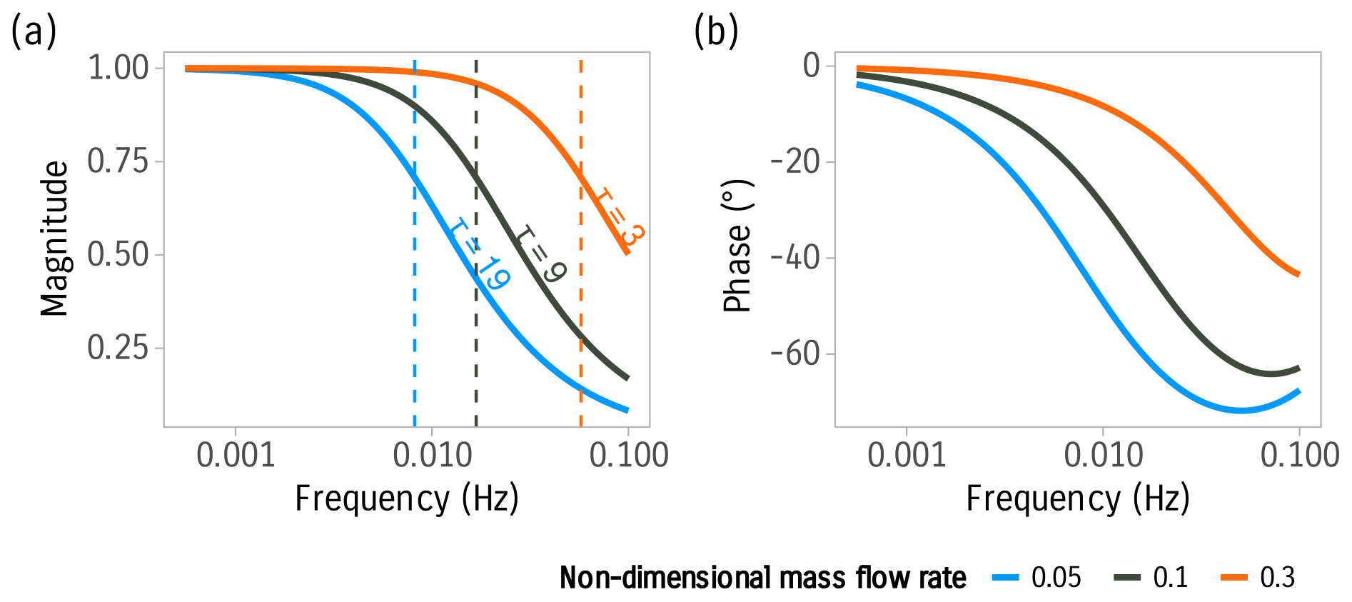
Figure 1Frequency response for the first-order linear filter used to model the buffer volumes for three different time constants. (a) Magnitude response of the filter. Vertical dashed lines represent the cutoff frequencies for the respective time constants. (b) Phase response of the filter.
3.1 Experimental site
Flux measurements were performed over a flat agricultural field of the Thünen Institute, located at 52.297∘ N, 10.449∘ E in Braunschweig, Germany. The site has an altitude of 76 m above sea level. During the measurement period, the fields south and north of the tower were planted with oats and corn, respectively. Both crops had a similar height of approximately 50 cm above the ground at the start of the comparison period.
3.2 Experiment period
Fluxes were measured throughout the year 2020. We selected 6 weeks of good quality in summer based on instrument performance and weather conditions, spanning from 18 June 2020 to 31 July 2020, to compare the different methods. Meteorological conditions (Fig. 3) during the experimental period from 18 June to 31 July 2020 were characterized by warm weather conditions with net radiation peaking around 600 W m−2 at noon. Air temperature was predominantly above 10∘ and averaged 18∘. Several precipitation events were observed during the experiment period. Precipitation totaled 66 mm, with several high precipitation events, in particular starting from the second and third weeks of the experiment. Precipitation data were obtained from the German weather service (DWD) station i Braunschweig (number: 00662), which is located 600 m from the measurement tower. Soil water content tracked precipitation events except for one distinct occasion on 27 June when precipitation is not registered at the DWD station. Wind direction was dominated by southerly and easterly winds.
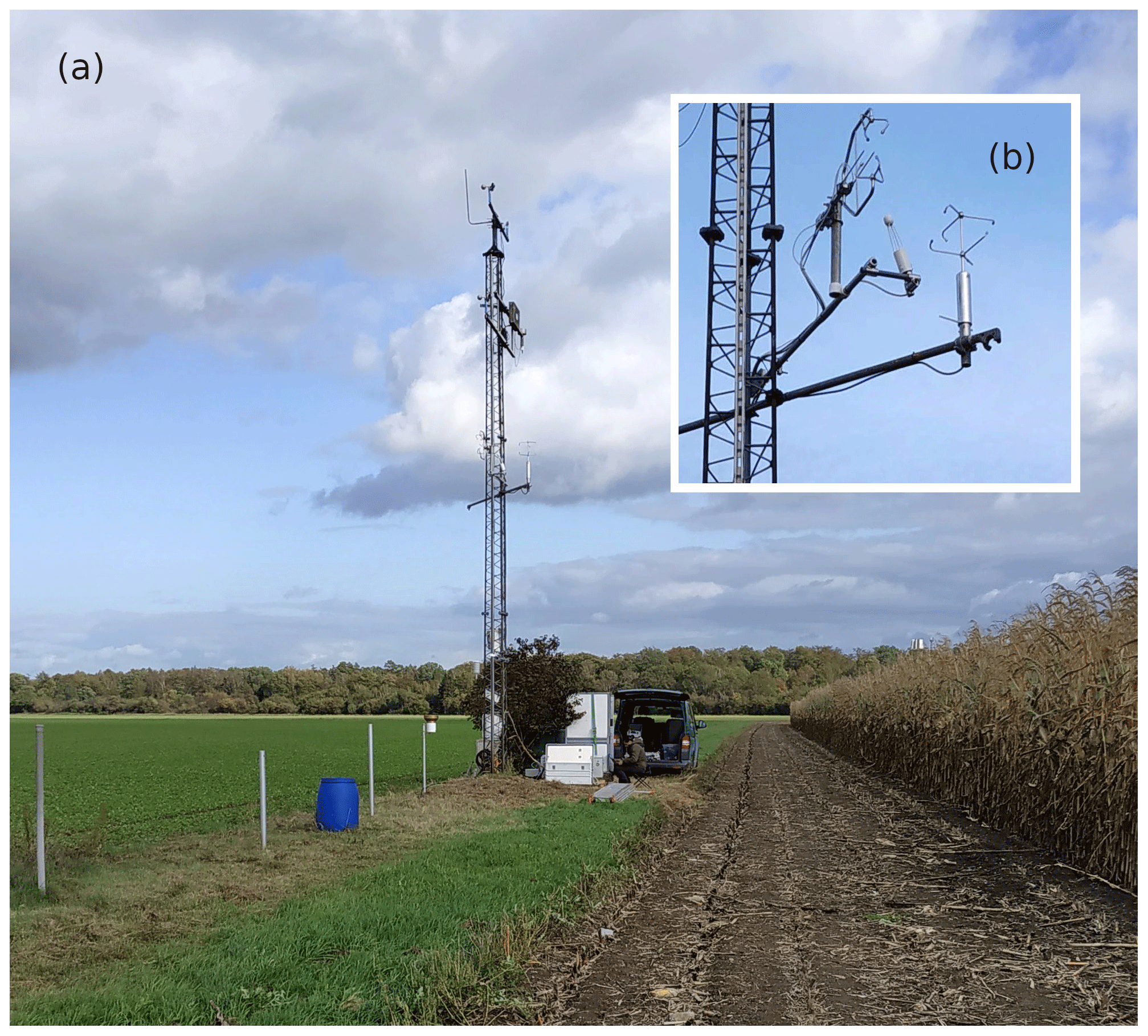
Figure 2Photograph of the experimental field site showing the measurement tower (a) and a close-up of the flux instruments mounted on the tower (b). The status of the vegetation seen in the picture is not representative of the measurement period.
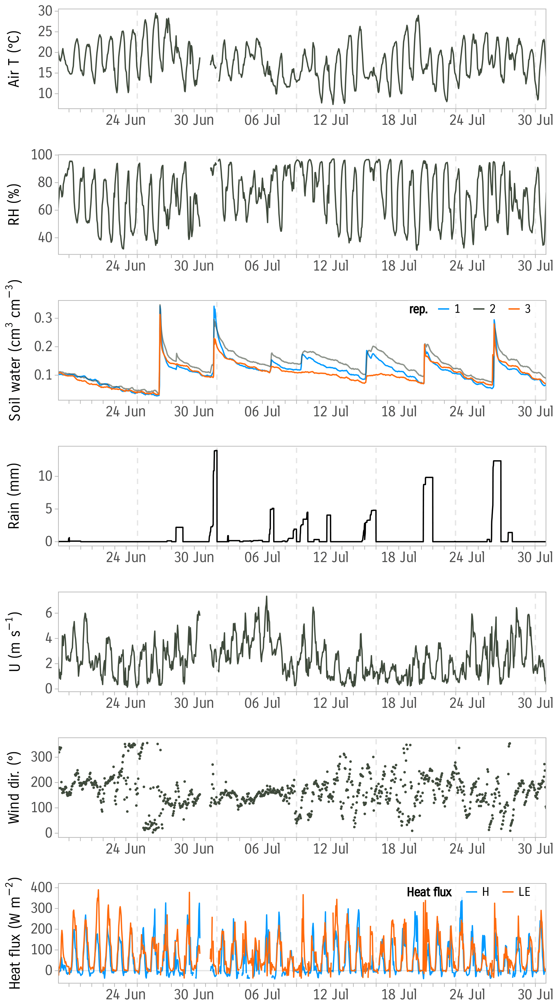
Figure 3Meteorological conditions and turbulent energy fluxes during the experiment period from 18 June to 31 July 2020: air temperature, relative humidity, soil water content, cumulative daily precipitation, wind velocity, wind direction, sensible heat flux (H), and latent heat flux (LE). Precipitation data were obtained from the German weather service (DWD) station in Braunschweig (number: 00662), which is located 600 m from the measurement tower.
3.3 Instruments
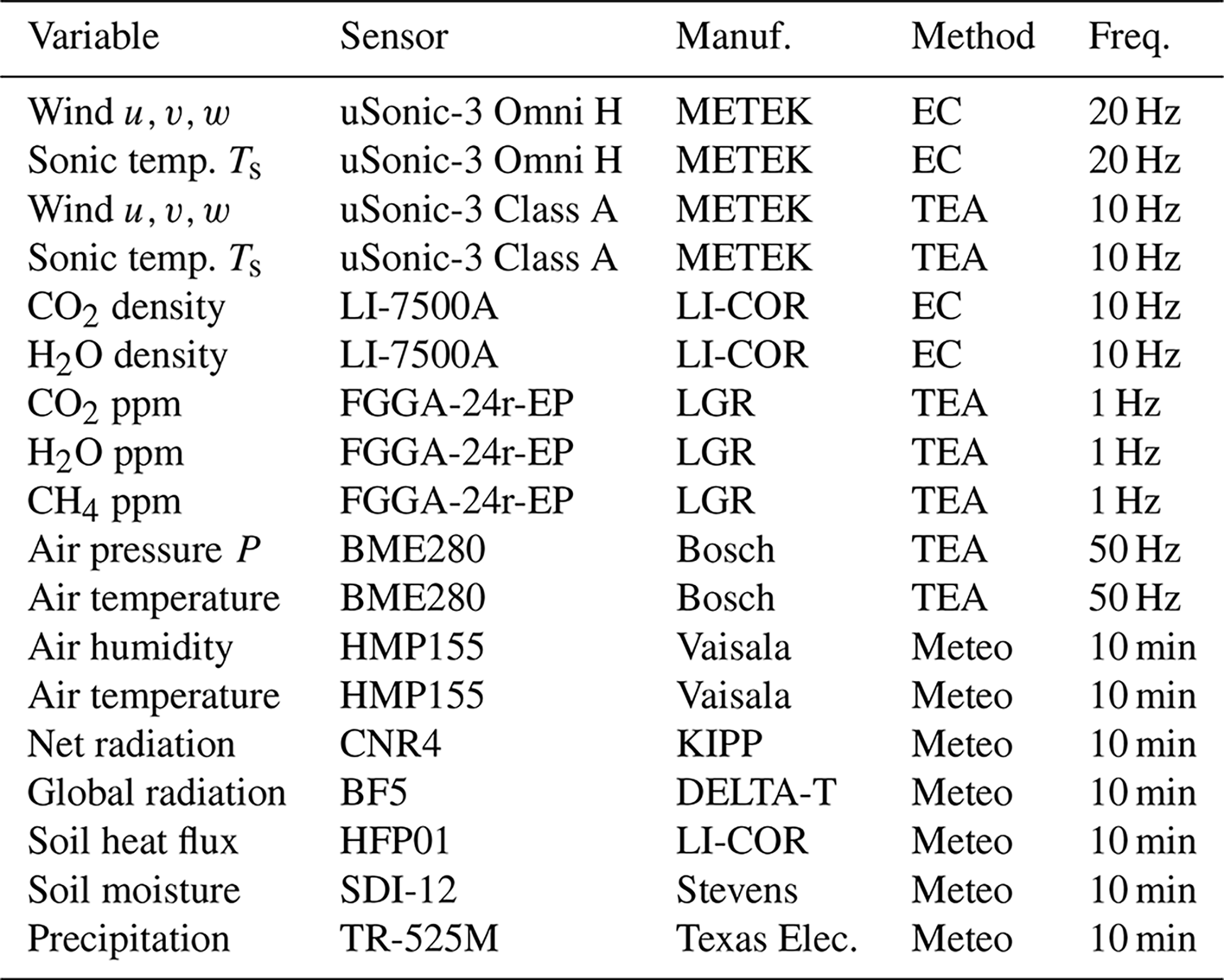
EC and STEA measurement complexes were mounted at 5 m height above the ground (Fig. 2). The instruments used in the experiment for flux measurements and data analysis are listed in Table 1. Meteorological variables were logged using a Sutron 9210 XLite logger (Sterling, USA). All the raw data needed for flux processing were synchronized on the STEA computer and remote servers for real-time processing.
Table 1Variables and instruments. Manufacturer key: METEK GmbH (Elmshorn, Germany), LI-COR Environmental Inc. (Lincoln, Nebraska, USA), LGR, (Los Gatos Research Inc., USA), Bosch (Bosch Sensortec GmbH, Germany), Vaisala (Helsinki, Finland), Kipp & Zonen (Delft, the Netherlands), Delta-T Devices Ltd (UK), Stevens Water Monitoring Systems, Inc (Oregon, USA), Texas Electronics (Dallas, USA).
The EC system comprised a dedicated sonic anemometer (uSonic-3 Omni H) and an open-path infrared gas analyzer (IRGA). Wind and scalar density data were acquired at 20 Hz frequency. Relative to the Class-A sonic anemometer used for STEA, the northward, eastward, and vertical separation of the IRGA was −17, 26, and −15 cm, respectively. The Class-A sonic anemometer had a north offset azimuth of 90∘. Relative to the Omni sonic anemometer used for EC, the northward, eastward, and vertical separation of the IRGA was 20, −15.3, and −20 cm. The north offset of the Omni sonic anemometer was 169∘.
3.4 STEA system description
The STEA system used in the experiment is based on an earlier system of Siebicke and Emad (2019). The new system used the same mass flow controllers and shared most of the operating software. It has, however, several differences and improvements. One major difference is the use of fixed stainless-steel buffer volumes instead of expandable bags. The system was initially developed as a hybrid TEA–EC method to run the TEA method in a continuous flow-through mode (Siebicke, 2016). The system was set up to operate in the STEA continuous flow-through mode. A constant duration for the short intervals (τi) equal to 1 min was used. The STEA system is comprised of two identical sampling lines, one for updrafts and one for downdrafts. Each of the sampling lines has two rigid buffer volumes in a sequence connected using 6 mm Teflon tube (Fig. 4).
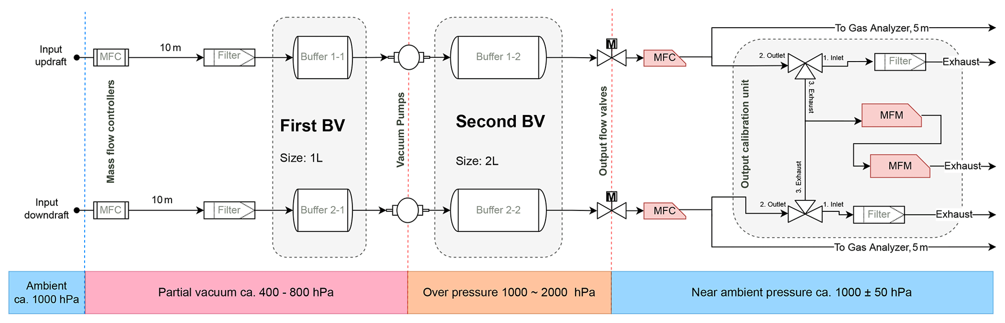
Figure 4Functional and pneumatic schematic of the implemented flow-through STEA system showing components, layout, properties, and operation conditions. Air samples are collected at the input and travel in distinct sampling lines for updrafts and downdrafts. Samples travel through tubes (lengths are shown) and through filters and are then collected into two sets of buffer volumes shown here as “first BV” and “second BV” separated by two vacuum pumps. The “output flow valves” followed by mass flow controllers (MFCs) control the output flow rate from the second set of buffers to the gas analyzers. Finally, samples can optionally be forwarded to a set of mass flowmeters (MFMs) used for calibration purposes. The colored bottom bar below shows the range of pressure values at each stage.
The STEA sampling inlets were installed near the sonic anemometer's center of the measurement volume. The horizontal separation was 22 cm, while the vertical separation between the two inlets was 2 cm. Upon sampling, the collected samples were carried using 6 mm Teflon tubes to the first set of buffers. The sampling can be summarized in the following steps (see a detailed description of the system operation and sampling in Siebicke and Emad, 2019).
-
3D wind measurements are acquired from the sonic anemometer (uSonic-3 Class A) with a 10 Hz sampling frequency.
-
Wind coordinates are rotated into the streamline coordinates using the planar fit method without an intercept (Dijk et al., 2004). The fit is performed online as a running window operation with a window width of 2 d and an update frequency of once every 30 min.
-
The mean vertical wind from the previous 30 min interval is removed to minimize . This is equivalent to applying a high-pass filter to the vertical wind velocity measurements.
-
The active sampling line is determined (updraft or downdraft) based on the direction of the rotated vertical wind velocity component.
-
The sampling scaling factor Ai is calculated based on wind conditions in the near past and the calibration coefficients of the mass flow controllers. The scaling factor should be constant during the short accumulation intervals.
-
Air samples are collected, and the controllers are adjusted to collect an air sample with a volume equal to Ai |w|.
-
When enough sample volume is accumulated in the respective buffer volume, samples are forwarded to the gas analyzer for analysis. The amount of sample volume needed is determined based on the required flow rate for the gas analyzer and the time needed to flush the tubes and the measurement cell as well as to perform enough repeated measurements.
-
Mean concentrations of accumulated samples are measured. The slow gas analyzer (LGR FGGA-24r-EP) alternates measuring the concentrations Ci of the accumulated samples for updraft and downdraft. The accumulation time for the short intervals was set to a fixed interval of 1 min instead of an adaptive interval duration. During each short interval, the gas analyzer performs repeated measurements for the gas concentration. The observed variability for repeated measurements in the short averaging intervals was SD = 0.501 ppm, which was similar to the measured repeatability of the gas analyzer for a similar time interval.
3.5 STEA flux computations
This section describes the steps followed to obtain the final and corrected STEA flux. Firstly, we discuss the effect of water vapor on the measured concentrations of other scalars and how we corrected the remaining water cross-sensitivity. Then, we present the procedure of data quality screening. Next, we detail the steps of calculating the final STEA flux. Finally, we present the buffer volume empirical correction we applied.
3.5.1 Water vapor correction
The gas analyzer used for the STEA measurements (LGR FGGA-24r-EP) reports the molar fraction of CO2 and CH4 of moist air in parts per million (ppm). The measurements of CO2 cannot be used directly, as they are affected by the presence of water vapor. The presence of varying water vapor concentrations in the sample affects the measurements of CO2 and CH4 in cavity ring-down spectroscopy instruments in at least two ways: (i) the dilution effect and (ii) spectroscopic line broadening (Rella, 2010). Rella (2010) proposed a quadratic equation to correct for the combined effect of line broadening and water vapor dilution. The correction involves estimating the parameters (a) and (b) in the equation
where rc is the dry mole fraction of the species c, χc is the wet mole fraction measured by the instrument, and χw is the water mole fraction measured by the instrument. For CO2 measured by the LGR gas analyzer in parts per million, Hiller et al. (2012) experimentally estimated these coefficients as and . We found that using the same parameters could not control for all the effects of water vapor on measured CO2 signals. A linear slope different from zero was still found when supplying the gas analyzer with air of varying water concentration and of constant CO2. This suggested a remaining cross-sensitivity of CO2 to the presence of water vapor. To control for this small remaining cross-sensitivity, we conducted a field experiment in which we measured the CO2 concentration in air of varying water concentration and then used the results in a linear fit to obtain a correction slope. We were not able to source the necessary equipment and gas cylinders to supply the gas analyzer with air of known CO2 concentration and varying water vapor in the field. Instead, we used the system's buffer volumes to collect and pressurize ambient air from the atmosphere, closed the inlets, and supplied the gas analyzer with enough sample flow rate for measurement. This procedure utilizes the effect of air drying due to decompression to deliver a varying water vapor content. The experiment involved collecting ambient humid air near saturation (RH ≈90 %, T=21 ∘C) in the system's buffer volumes to a pressure of 2.6 bar. As a result of the high pressure, the water partial pressure in the pressurized buffer volumes will become higher than the saturation vapor pressure and water will precipitate, leading to dryer air. Air is then decompressed and forwarded to the analyzer. As the buffer pressure is decreasing, water vapor content will increase to reach the same level of atmospheric humidity. Using this method we were able to modulate the water vapor content in the air from 6000 to 14 000 ppm. The accumulated sample was enough to supply the gas analyzer for ca. 10 min. We repeated the measurements several times and used the obtained dataset to correct the remaining cross-sensitivity using a linear fit.
3.5.2 Raw data quality screening
Raw measurements of the wind velocity and scalar concentration were screened for outliers due to measurement errors and instrument malfunction. This included the following steps.
-
Statistical screening: despiking, dropout removal (Vickers and Mahrt, 1997), and plausibility limits of the raw gas analyzer and wind measurements (Sabbatini et al., 2018).
-
Flushing time removal: measurement of the short interval events involves regularly switching the sampling line coming to the gas analyzer between updraft and downdraft reservoirs. This caused subsequent samples to get contaminated. We experimentally chose a 25 s threshold at the start of each short interval event to account for the flushing time. The measurements falling before the threshold were discarded. Figure 5 shows an example of discarded flushing times at the start of each averaging interval.
-
Detection of sample contamination: periods during which the flow rate to the gas analyzer is smaller than 400 mL min−1 are flagged. Under these conditions, ambient air might enter the system and contaminate the collected samples. When the number of flagged data points exceeded 10 % of the total points in the sampling interval, data in the sampling interval were discarded.
3.5.3 STEA flux calculation
After measurements are quality-checked and erroneous data points are excluded, the final STEA flux is calculated as follows.
-
Short interval statistics: for each short interval sample, the gas analyzer will have several repeated measurements for the concentrations Ci. However, only one value is needed for the flux calculation. We use the median to obtain the representative value in order to minimize uncertainty and exclude outliers. Figure 5 shows an example of data quality checking and choice.
-
Calculate air molar volume: the molar volume of air is needed to express the flux in units of . The molar volume is calculated using sonic temperature, pressure, and humidity measurements.
-
Calculate short interval weights: following Eq. (6), the measured short interval concentration should be weighted by the ratio of the accumulated volume during that interval to the total buffer volume.
-
Calculate values of αθ: values of the transport asymmetry coefficient αθ are calculated using vertical wind velocity and sonic temperature measurements. Values of αθ larger than 1 are discarded as they indicate a problem with the measurement as discussed in the companion paper (Emad and Siebicke, 2023).
-
Calculate updraft and downdraft mean concentrations: and are calculated for the averaging period Δt.
-
Calculate the flux: the STEA flux equation shown in Eq. (7) is used to obtain the final flux.
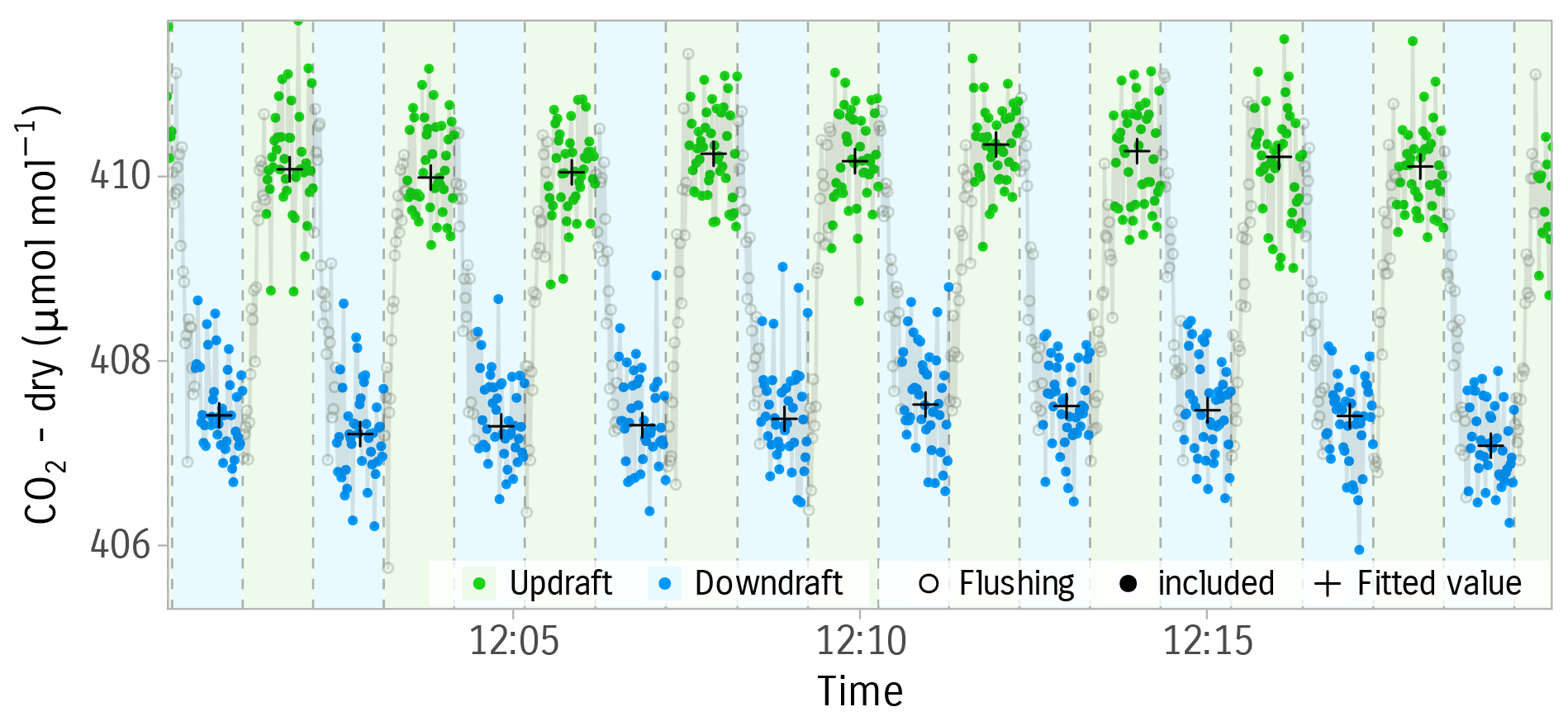
Figure 5Data choice and fitting procedure for the STEA method. Points represent consecutive concentration measurements from the gas analyzer. Updraft and downdraft samples are highlighted in blue and green, respectively. Gray hollow points are excluded from the data fitting (flushing time). Crosses show the chosen representative concentrations for each short interval (the median). Further quality checks for raw data are outlined in Sect. 3.5.2. Data are from 21 June 2020 at midday.
3.5.4 Buffer volume empirical correction
Buffer volumes act on the signal as a low-pass filter and introduce systematic bias to the fluxes. We used Eq. (10) to estimate the time constant of the buffer volumes used in our experiment. For each of the buffer volumes, a measurement point is acquired every 2 min. The mean dimensionless mass flow rate to the gas analyzer was estimated from the pressure, the volume, and the estimated volumetric flow rate to the gas analyzer. We simulated the effect of buffer volumes on the high-frequency sonic temperature signal and parameterized the flux loss by artificially degrading the sonic temperature in a procedure similar to Goulden et al. (1996) and Berger et al. (2001).
3.6 EC reference flux measurements and computations
The raw data from the two sonic anemometers and the high-frequency gas density measurements from the IRGA were used to compute eddy covariance fluxes for water vapor and CO2 in the period from 1 April 2020 to 1 November 2020 using EddyPro® software (LI-COR Env. Inc. USA) version 7.0.4. The flux processing steps were chosen to be as similar as possible to the STEA processing scheme. The calculation of EC fluxes involved statistical screening for the data quality issues following Vickers and Mahrt (1997), mean removal by block averaging, compensation for the time lag between the wind and the scalar time series using covariance maximization, tilt correction using the planar fit method without an intercept (Dijk et al., 2004) similar to STEA, and analytical high- and low-frequency corrections to correct for the spectral attenuation of the IRGA (Moncrieff et al., 2005, 1997).
3.6.1 Density fluctuation correction
Due to using a closed-path gas analyzer, the TEA and STEA methods do not require the WPL (Webb, Pearman, and Leuning) correction (Webb et al., 1980). WPL accounts for the effect of density fluctuations due to changes in temperature, humidity, and pressure. In TEA and STEA, after samples are collected and mixed in buffer volumes, the mean mixing ratio is measured. Therefore, no correction for density effects is needed as long as accurate mass flow sampling of air is maintained. The measured TEA and STEA flux is equivalent to the flux measured with mixing ratios .
3.7 Data selection for method comparison
To compare the fluxes calculated from both methods, we selected averaging intervals according to the following criteria.
-
Spike removal: this is done following Vickers and Mahrt (1997) using a window width of 6 h and a threshold of 2 standard deviations. This was mainly to account for unreliably elevated CO2 concentrations recorded by the open-path gas analyzer due to water condensation.
-
Rainy period exclusion: data records during rainy weather conditions were excluded.
-
Flux quality flags: periods when the flux quality flag is 1 or 2 according to Foken et al. (2005) were excluded.
-
STEA low flow rate: averaging intervals flagged with the low flow rate flag described earlier were discarded.
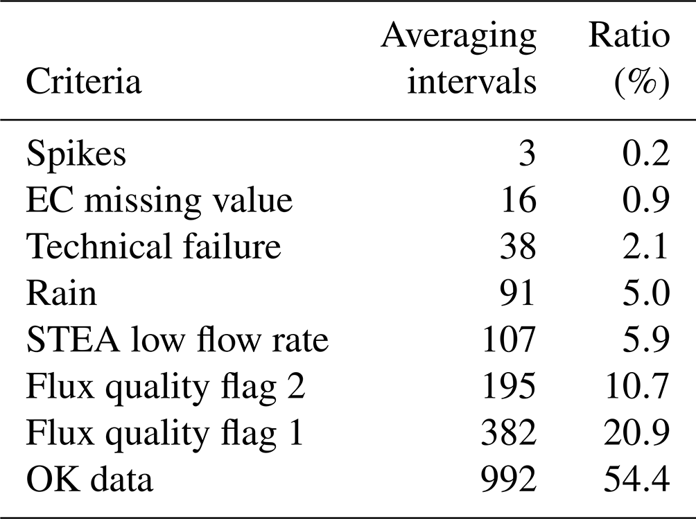
After applying the above criteria, 992 averaging intervals remained. They accounted for 54.4 % of the whole comparison period. Nighttime data were the majority of excluded values with only 33 % of averaging intervals valid during nighttime compared to 70 % during daytime. The open-path gas analyzer used for EC produced unreliable measurements during high humidity conditions at night due to water condensation. Table 2 shows a summary of data quality-check results.
Table 2Summary of data quality checks for STEA and EC fluxes used in the EC–STEA flux intercomparison showing the number of averaging intervals that were excluded and the ratio of the excluded averaging intervals to the total for each criterion. Details on the criteria and the thresholds used are provided in Sect. 4.3.
To compare the overall difference between the two methods, we used the coefficient of determination R2 and the slope of the orthogonal distance regression (ODR) (also known as major-axis regression and model II regression). ODR considers the errors in x and y as opposed to ordinary least squares (OLS) regression, which assumes that the error in x is negligible (Wehr and Saleska, 2017).
We first discuss the newly proposed short-time eddy accumulation method. Then, we discuss some results and aspects of the STEA flux calculations. Afterward, we present the flux intercomparison between STEA and EC. Finally, we discuss the effect of using fixed buffer volumes on the fluxes and the proposed empirical correction.
4.1 Short-time eddy accumulation
Using the STEA method reduced the dynamic range requirement for eddy accumulation sampling. For a short averaging interval of 1 min, the range was on average 60 % of the range required for the conventional eddy accumulation. As a result, the upper bound of the required dynamic range for w reported by Hicks and McMillen (1984) as 5 σw is lowered to 3 σw. The reduction of the required dynamic range improves the accuracy and performance of the STEA system. The accumulation on shorter timescales brings many advantages. First, it allows adapting to the local range of vertical wind velocity values, which improves the resolution and dynamic range of the system. This can be achieved by exploiting the autocorrelation of the wind velocity signal to predict a scaling parameter, Ai, better adapted to the local velocity field for each interval. For a short interval, the range that the sampling apparatus needs to cover will be smaller on average than the range of the whole averaging interval.
Additionally, the accumulation on varying intervals means the measurement frequency can be adjusted to match that of the gas analyzer or the precision requirements. This can be useful for reactive species and other trace gases, for which relatively fast gas analyzers are available but not fast enough for EC.
Figure 6 demonstrates how the STEA method works. In this example, the high-frequency samples are collected at 5 Hz frequency for a 30 min averaging interval. The averaging interval is divided into 30 short intervals with a duration varying from 70 to 190 s. The flux in this example equals −14.24 .
Finally, the STEA method facilitates using the STEA system in a continuous flow-through mode using rigid reservoirs. The operation in flow-through mode requires two sets of buffer volumes in a series as shown in Fig. 4, with two buffer volumes for each sampling line. The ideal operation of such a system can be achieved as follows.
-
Wind velocity is measured and rotated, and the value of the scaling parameter Ai is updated based on wind statistics and the flow calibration parameters.
-
For each sampling line, air samples are collected into the respective set of buffer volumes continuously according to the sign of the vertical wind velocity and proportional to its magnitude and the value of Ai until a predefined accumulated volume is reached.
-
When the predefined accumulated volume is reached, the second buffer volume in the sampling line is disconnected from the first. Sample accumulation time, τi, and accumulated mass are recorded. Then, samples are forwarded to the gas analyzer.
-
The slow gas analyzer alternates measuring scalar concentration for each interval Ci from the second set of buffer volumes for updraft and downdraft.
The successful use of this scheme requires keeping the mass flow rate of air from the second set of buffer volumes to the gas analyzer constant for consecutive short intervals since the model used to represent the buffer volumes in Eq. (8) assumes the flow rate to be constant with respect to time.
4.2 STEA fluxes computations
In this section, we discuss some aspects related to the calculation of the STEA fluxes. We first discuss the effects of water vapor on CO2 concentration measurements. Then, we discuss the effect of coordinate rotation on the fluxes.
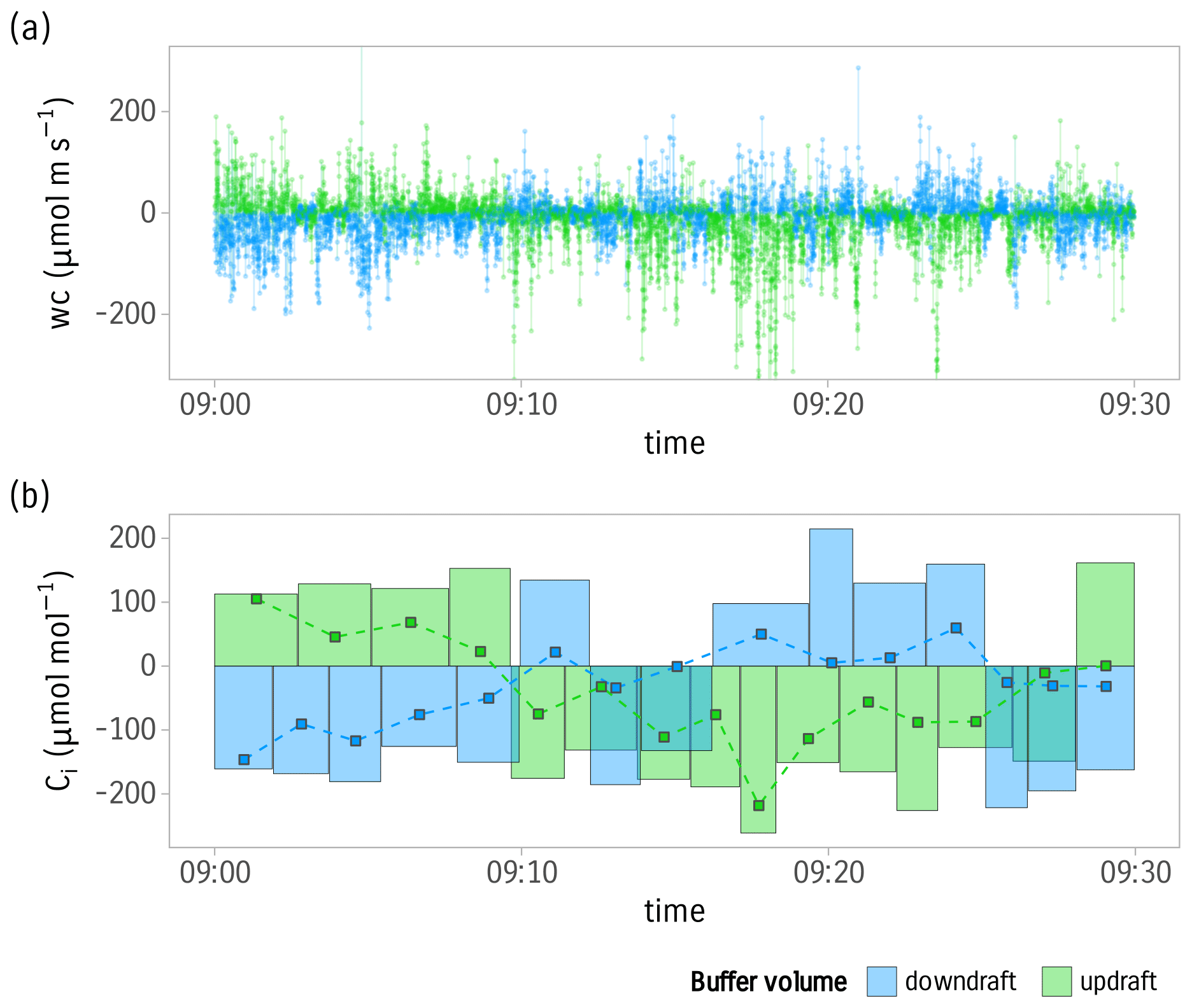
Figure 6Sample accumulation using the STEA method. An example of 30 min of measurements: (a) samples wc are collected based on wind direction and proportional to its magnitude. (b) Short intervals are accumulated. The variable short interval duration guarantees equal accumulated volume for consecutive short intervals. Points are the concentrations Ci measured by the gas analyzer. The area of each rectangle represents the accumulated sample volume in arbitrary units and is equal to the relative weight for each concentration measurement. The sum of all measurements Ci weighted by the relative sample volume will equal the covariance. Data are from 20 June 2020.
4.2.1 Water vapor correction
Treatment of the residual cross-sensitivity of CO2 to water vapor content using a linear fit produced a small slope of shown in Fig. (7). Thus, a difference in water concentration of 4000 ppm between updraft and downdraft reservoirs, typically observed in extreme conditions, will lead to a difference on the order of 0.5 ppm for CO2. Applying the water vapor correction using the quadratic fit and the slope correction reduced the magnitude of STEA fluxes in comparison to the direct calculation of mixing ratios. However, it improved the fit between the STEA and the reference EC flux (slope decreased from 1.18 to 1.04, and R2 increased from 0.80 to 0.86).
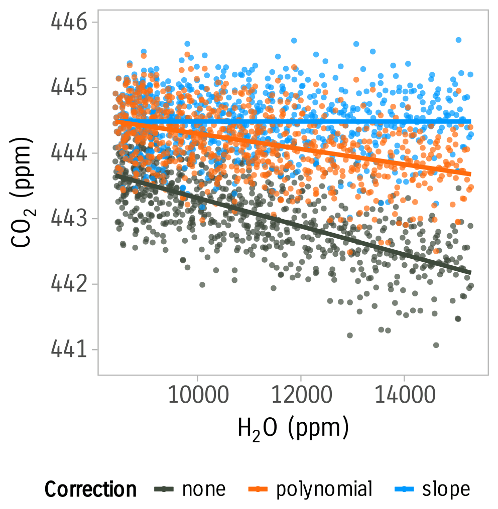
Figure 7Effect of water correction on the measured CO2 concentration using the LGR FGGA-24r-EP instrument. Points represent measured CO2 by the gas analyzer when air with constant CO2 concentration and varying H2O concentration was supplied. Lines represent linear regression fits. Red-colored points and the red line represent CO2 measurements after applying the polynomial correction (Hiller et al., 2012; Rella, 2010). In blue are the CO2 measurements after applying our slope adjustment correction to remove additional cross-sensitivity to water.
4.2.2 Coordinate rotation
The online coordinate rotation produced rotation angles with low variability over the experiment period. The eddy covariance fluxes calculated using the Class-A sonic anemometer with a 2-month-long dataset (1 June 2020 to 1 August 2020) produced the following rotation angles: x − pitch = 0.6∘; y − roll = −4.3∘ (using the YXZ Euler convention), whereas for the TEA moving-window online rotation, larger pitch angles were observed with a mean of 3.6∘ and values slowly climbing from 1.2 to 6∘ during the 6-week comparison period. The roll angle ranged from −0.9 to −0.24∘ with an average of −0.4∘.
The use of online rotation with a moving window of 2 d minimized the residual mean vertical wind in comparison to using the whole period of the experiment. This is likely due to a better adaptation to the local wind field. Furthermore, the distribution of normalized mean vertical wind velocity of the short moving window had less spread and thinner tails, and it showed more symmetry around the mean compared to the whole-dataset rotation. The residual mean magnitude of rotated w for the short moving window was 0.04 σw. The first and third quartiles were −0.03 and 0.03 σw, whereas for the whole-dataset rotation, the mean magnitude was 0.17 σw and the first and third quartiles were −0.07 and 0.22 σw, respectively.
To estimate the effect of the online rotation method on the fluxes, we calculated EC fluxes using the two different rotation approaches while keeping other treatments constant. The comparison revealed that the online rotation with a moving window had a minimal effect on the fluxes: a slope of approximately 1 and an R2 of 0.98 were obtained when using a linear fit. Nevertheless, this comparison only included data of good quality from an ideal site. These results might differ for nonideal conditions at a more complex site.
4.3 STEA–EC flux intercomparison
The measured CO2 fluxes using the STEA method in flow-through mode showed a good match with the reference EC fluxes (Fig. 8).
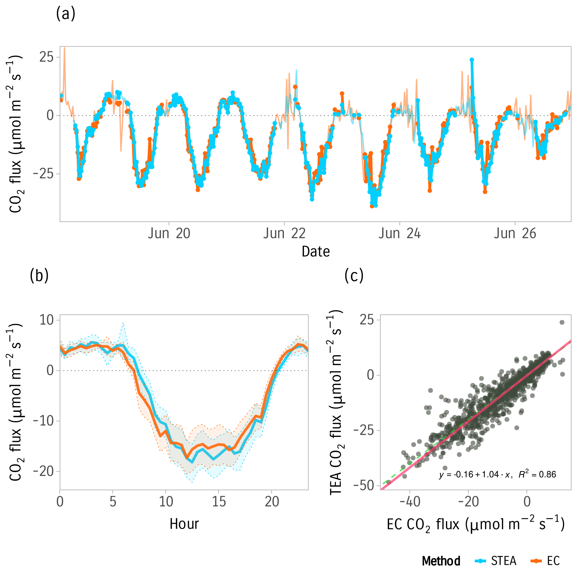
Figure 8STEA and EC flux intercomparison. (a) Time series of EC and STEA CO2 fluxes for a subset period of 9 d. Points and thick lines indicate the averaging intervals used for comparison after filtering for quality. (b) Mean diurnal cycle of CO2 fluxes of STEA and EC. Bands are 95 % confidence intervals of the mean calculated using nonparametric bootstrapping. (c) Scatter plot of STEA CO2 fluxes against reference EC fluxes. The red line is the linear fit using orthogonal distance regression (ODR). The dashed green line is a 1-to-1 line for reference. Data used for panels (b) and (c) are from 18 June to 31 July 2020, while for panel (a) a 9 d subset from 18 to 27 June 2020 was used.
The time series of measured CO2 fluxes in Fig. (8a) shows that the STEA method was able to reproduce the daily dynamics of CO2 flux very well. The estimated fluxes using the STEA method appear to have fewer spikes and are smoother in general; this is likely due to the smoothing effect of buffer volumes and the lower sensitivity of the closed-path gas analyzer to rain and high humidity, in particular during nighttime. The correction for nonzero mean vertical wind velocity using αθ was on average less than 1.5 % of the flux magnitude. This is due to the ideal topography of the site and the online rotation of the coordinates. The correction at less ideal sites with more complex topography may differ.
The mean diurnal cycle estimates from the two methods match very well (Fig. 8b). However, a small time shift can be observed in the mean diurnal cycle as a result of the phase shift introduced by the low-pass-filtering effect of the buffer volumes.
The linear regression in Fig. 8c shows that the measured CO2 fluxes using the STEA method in flow-through mode have very good agreement with the reference EC fluxes. The magnitude of STEA fluxes was comparable to EC fluxes (ODR slope = 1.04). This indicates that the STEA method does not introduce systematic error to the fluxes.
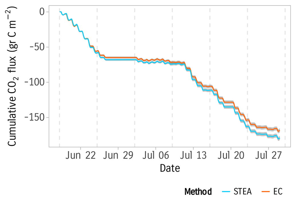
Figure 9Cumulative fluxes of STEA and EC during the experimental period from 18 June to 31 July 2020. Bands represent the flux random error (2σ) estimated from the random sampling error of the EC fluxes. Only data with good quality were used, and no gap filling was applied.
Cumulative fluxes for the entire 6-week experiment period show generally good agreement between STEA and EC (Fig. 9). The cumulative CO2 flux was estimated to be gr C m−2 using EC and 179.3±1.42 gr C m−2 using STEA. The difference between the two methods is −10.9 gr C m−2, which is about 6 % of the cumulative flux. While this difference falls slightly outside the uncertainty of the two methods, we note that the uncertainty estimates are based on the sampling error only and do not include other sources of uncertainty such as the different gas analyzers, the different data treatments, and the additional uncertainty contributions of sampling and buffers volumes in STEA. Furthermore, the difference between the two methods seems to increase in the last 3 weeks of the experiment, which coincides with intermittent rainfall and more variance in wind direction. Therefore, we believe this difference does not indicate a systematic error in the flux estimates.
The coefficient of determination of the measured fluxes during the whole experiment period R2 was 0.86. The remaining 13 % of unexplained variance is the joint contribution of the uncertainties of the two flux estimates from the EC and STEA methods. The observed uncertainty from the two methods calculated as the standard deviation of the difference was 4.36 . We suggest three different mechanisms contributing to the observed uncertainty leading to the unexplained variance between the two estimates. First, the random sampling error arising from the stochasticity of turbulence (Hollinger and Richardson, 2005). The mean random sampling error of EC fluxes calculated following Finkelstein and Sims (2001) was 1.58 . The standard deviation of the difference between the two methods can be estimated to be 2.34 if STEA fluxes are assumed to have a similar random sampling error. Therefore, the random sampling error of the two methods accounts for more than half of the observed variance. The difference between the two methods also shows heteroscedasticity, with the error increasing along with the absolute magnitude of the flux; a similar behavior of the random sampling error was observed by Hollinger and Richardson (2005) when comparing two tower estimates. The second source of uncertainty is the use of different gas analyzers for STEA and EC. Polonik et al. (2019) compared five different analyzers for measuring CO2 fluxes. They showed that the root mean square error (RMSE) was in the range of 1 to 3.35 depending on the analyzer type and the spectral correction method applied, with larger discrepancies observed when comparing open-path to closed-path sensors. Our results have an RMSE value of 4.39 . While our result is slightly higher, it should be noted that RMSE is not an ideal metric for cross-study comparison. A relative metric, such as R2, would be more comparable but was unavailable. The third source of uncertainty is the use of buffer volumes in the STEA method. Figure 10a demonstrates the increase in scatter in the measured fluxes due to the use of buffer volumes. Finally, the different processing steps between the two methods can contribute to the uncertainty, in particular the effects of time-lag compensation, spectral corrections, and statistical screening. We determined the combined effect of these processing treatments by calculating the EC flux with and without the treatments and found that the systematic errors in the flux were negligible.
4.4 Effect of buffer volumes
Using fixed buffer volumes attenuates the signal. To understand the effect of buffer volume use on the measured scalar concentration, we carried out a simulation on a surrogate signal generated from sonic temperature. The simulation showed that buffer volumes caused a decline that can reach up to 10 % of the fluxes under operation ranges similar to those of our experiment (for τ=11 min) (Fig. 10). The empirical correction was consistently able to mitigate most of the attenuation when the filter properties are assumed to be constant (i.e., the flow rate needs to be constant for consecutive short intervals). This assumption was difficult to maintain using the 1 min switching regime. The simulation showed that the empirical correction for the buffer volumes worked best when the correction factor was obtained using a linear fit, as opposed to taking a ratio of the attenuated flux to the true flux for each averaging interval. The correction factor, in this case, is the reciprocal of the slope of the linear regression between the attenuated flux and the true flux. The correction factor calculated using Eq. (10) shows good agreement between sensible heat flux and CO2. However, the uncertainty of the correction factor increased with increasing buffer volume time constant. For our experiment, the average time constant for the first-order linear filter used to model the buffer volume was estimated to be τ=700 s. This value was used to simulate the loss on the fluxes using the sensible heat flux calculated from the sonic anemometer. The correction factor was obtained from the slope of the attenuated flux and was equal to 1.18.
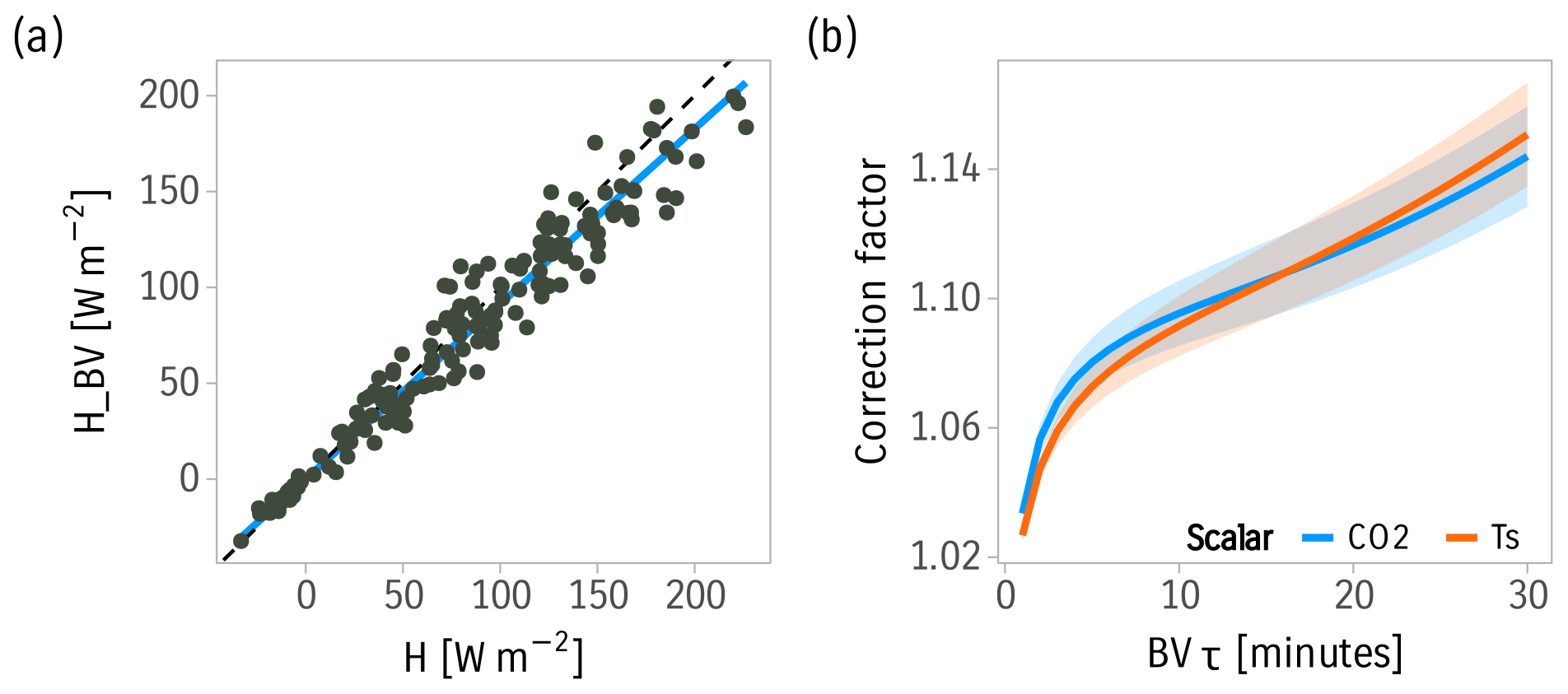
Figure 10Empirical buffer volume correction. (a) Effect of buffer volume attenuation on sensible heat flux with a time constant τ=11 min. The blue solid line is the linear fit between the two. (b) Empirical correction factor for the effect of buffer volumes calculated as the reciprocal of the slope of attenuated flux for CO2 and sensible heat flux. Bands are the estimated slope ± 1 standard error of the slope.
The empirical correction scheme achieved here by simulating the loss on sensible heat flux lacks a proper treatment of the phase shift introduced by the first-order filter. Additionally, the similarity of transport between sensible heat flux and CO2 is an approximation that is expected to be valid only on average as evidenced by the large scatter around the regression line in Fig. 10. Therefore, a direct correction that can estimate the original signal before attenuation is needed. Such a correction has since been developed and is the topic of a future publication (Emad, 2022).
In this paper, we proposed a new variety of the eddy accumulation method as an alternative to eddy covariance for the measurement of ecosystem-level fluxes. The new method, referred to here as short-time eddy accumulation (STEA), allows the sample accumulation to be carried out on shorter intervals of varying length. The STEA method offers more flexibility than the conventional TEA method and has many potential benefits. Most importantly, STEA provides a higher dynamic range and better accuracy than the TEA method and enables operating sample accumulation under a flow-through scheme using fixed buffer volumes. The flexibility introduced by the STEA method offers new ways to design eddy accumulation systems that are particularly suited for specific atmospheric constituent gas analyzers. For example, the accumulation time can be tailored to measure reactive species with lifetimes shorter than a conventional flux integration interval or to distribute the gas analyzer time to measure fluxes at different heights.
Furthermore, we presented a prototype evaluation of the STEA method under the flow-through regime. We described the details of the system design and operation. We compared flux measurements from our new system against a reference EC system over a flat agricultural field. The fluxes from the two methods were in very good agreement. We highlighted the importance of different processing and design aspects between the two methods and their potential effects on the fluxes.
Finally, we analyzed the effect of buffer volumes in the flow-through operational mode on the fluxes and proposed an empirical correction to correct for the underestimation resulting from the low-pass-filtering behavior of the buffer volumes.
In summary, the new STEA method provides a direct flux measurement method that complements the state-of-the-art EC method. It extends the coverage of micrometeorological methods to new trace gases and atmospheric constituents beyond the scope of the EC method.
| Symbols | ||
| c | mol m−3 | Molar density of a scalar |
| w | m s−1 | Vertical wind velocity |
| Δt | s | Flux averaging interval |
| A | – | TEA sampling scaling factor |
| V | m3 | Volume |
| C | mol m−3 | Mean concentration |
| of accumulated samples | ||
| αc | – | Transport asymmetry coefficient |
| for scalar c | ||
| ρ | – | Correlation coefficient |
| – | Dimensionless mass flow rate | |
| τ | s | Time constant of the buffer volume |
| rc | ppm | Mixing ratio in dry air for a scalar, c |
| Subscripts | ||
| acc | Accumulated samples | |
| ↑ | Updraft buffer volume | |
| ↓ | Downdraft buffer volume | |
| c | Atmospheric constituent |
The data and code required to produce the figures in this paper are provided at https://doi.org/10.5281/zenodo.7451511 (Emad and Siebicke, 2022).
AE developed the theory of the STEA method and the empirical correction for the effect of buffer volumes, implemented needed software, performed the experiment, analyzed the data, interpreted the results, and wrote the paper. LS conceptualized the idea of a flow-through eddy accumulation system, built the TEA system used in the experiment, planned and supervised the experiment, and provided feedback on the results, the analysis, and the paper.
The contact author has declared that none of the authors has any competing interests.
Publisher's note: Copernicus Publications remains neutral with regard to jurisdictional claims in published maps and institutional affiliations.
We gratefully acknowledge the support of the Bioclimatology group, led by Alexander Knohl at the University of Göttingen, in particular technical assistance by Justus Presse, Frank Tiedemann, Marek Peksa, Dietmar Fellert, and Edgar Tunsch. We thank Christian Brümmer and Jean-Pierre Delorme from the Thünen Institute for Agricultural Climate Protection and Mathias Herbst from the Center for Agrometeorological Research of the German Meteorological Service (DWD) for facilitating the fieldwork in Braunschweig. We further acknowledge Christian Markwitz for the fruitful discussions during the preparation of the paper and for reading and commenting on the paper. We thank Alexander Knohl, Nicolò Camarretta, Justus van Ramshorst, and Yannik Wardius for reading the paper and providing useful comments.
This research has been supported by the Niedersächsische Ministerium für Wissenschaft und Kultur (Wissenschaft.Niedersachsen.Weltoffen grant), the H2020 European Research Council (grant no. 682512 – OXYFLUX), and the Deutsche Forschungsgemeinschaft (grant no. INST 186/1118-1 FUGG).
This open-access publication was funded by the University of Göttingen.
This paper was edited by Hartwig Harder and reviewed by Christoph Thomas and one anonymous referee.
Baldocchi, D.: Measuring Fluxes of Trace Gases and Energy between Ecosystems and the Atmosphere – the State and Future of the Eddy Covariance Method, Global Change Biol., 20, 3600–3609, https://doi.org/10.1111/gcb.12649, 2014. a
Berger, B. W., Davis, K. J., Yi, C., Bakwin, P. S., and Zhao, C. L.: Long-Term Carbon Dioxide Fluxes from a Very Tall Tower in a Northern Forest: Flux Measurement Methodology, J. Atmos. Ocean. Technol., 18, 529–542, https://doi.org/10.1175/1520-0426(2001)018<0529:LTCDFF>2.0.CO;2, 2001. a
Businger, J. A. and Oncley, S. P.: Flux Measurement with Conditional Sampling, J. Atmos. Ocean. Technol., 7, 349–352, https://doi.org/10.1175/1520-0426(1990)007<0349:FMWCS>2.0.CO;2, 1990. a
Cescatti, A., Marcolla, B., Goded, I., and Gruening, C.: Optimal use of buffer volumes for the measurement of atmospheric gas concentration in multi-point systems, Atmos. Meas. Tech., 9, 4665–4672, https://doi.org/10.5194/amt-9-4665-2016, 2016. a
Desjardins, R. L.: Energy Budget by an Eddy Correlation Method, J. Appl. Meteorol., 16, 248–250, https://doi.org/10.1175/1520-0450(1977)016<0248:EBBAEC>2.0.CO;2, 1977. a
Dijk, A., Moene, A., and de Bruin, H.: The Principles of Surface Flux Physics: Theory, Practice and Description of the ECPACK Library, The Principles of Surface Flux Physics: Theory, Practice and Description of the ECPACK Library, 2004/1, 525–2004, Meteorology and Air Quality Group, Wageningen University, Wageningen, the Netherlands, 2004. a, b
Emad, A.: Optimal Frequency-Response Corrections for Eddy Covariance Flux Measurements Using the Wiener Deconvolution Method, PREPRINT – available at Research Square, https://doi.org/10.21203/rs.3.rs-2075158/v1, 2022. a
Emad, A. and Siebicke, L.:Reproduction Data and Code for the Paper: True Eddy Accumulation – Part 2: Theory and Experiment of the Short-Time Eddy Accumulation Method, Zenodo [data set], https://doi.org/10.5281/zenodo.7451511, 2022. a
Emad, A. and Siebicke, L.: True eddy accumulation – Part 1: Solutions to the problem of non-vanishing mean vertical wind velocity, Atmos. Meas. Tech., 16, 29–40, https://doi.org/10.5194/amt-16-29-2023, 2023. a, b, c, d, e
Finkelstein, P. L. and Sims, P. F.: Sampling Error in Eddy Correlation Flux Measurements, J. Geophys. Res.-Atmos., 106, 3503–3509, https://doi.org/10.1029/2000JD900731, 2001. a
Finnigan, J. J., Clement, R., Malhi, Y., Leuning, R., and Cleugh, H.: A Re-Evaluation of Long-Term Flux Measurement Techniques Part I: Averaging and Coordinate Rotation, Bound.-Lay. Meteorol., 107, 1–48, https://doi.org/10.1023/A:1021554900225, 2003. a
Foken, T., Göockede, M., Mauder, M., Mahrt, L., Amiro, B., and Munger, W.: Post-Field Data Quality Control, in: Handbook of Micrometeorology: A Guide for Surface Flux Measurement and Analysis, edited by: Lee, X., Massman, W., and Law, B., Atmospheric and Oceanographic Sciences Library, 181–208, Springer Netherlands, Dordrecht, https://doi.org/10.1007/1-4020-2265-4_9, 2005. a
Goulden, M. L., Munger, J. W., Fan, S.-M., Daube, B. C., and Wofsy, S. C.: Measurements of Carbon Sequestration by Long-Term Eddy Covariance: Methods and a Critical Evaluation of Accuracy, Global Change Biol., 2, 169–182, https://doi.org/10.1111/j.1365-2486.1996.tb00070.x, 1996. a
Gu, L., Massman, W. J., Leuning, R., Pallardy, S. G., Meyers, T., Hanson, P. J., Riggs, J. S., Hosman, K. P., and Yang, B.: The Fundamental Equation of Eddy Covariance and Its Application in Flux Measurements, Agr. Forest Meteorol., 152, 135–148, https://doi.org/10.1016/j.agrformet.2011.09.014, 2012. a
Hicks, B. B. and Baldocchi, D. D.: Measurement of Fluxes Over Land: Capabilities, Origins, and Remaining Challenges, Bound.-Lay. Meteorol., 177, 365–394, https://doi.org/10.1007/s10546-020-00531-y, 2020. a
Hicks, B. B. and McMillen, R. T.: A Simulation of the Eddy Accumulation Method for Measuring Pollutant Fluxes, J. Clim. Appl. Meteorol., 23, 637–643, https://doi.org/10.1175/1520-0450(1984)023<0637:ASOTEA>2.0.CO;2, 1984. a, b, c
Hiller, R. V., Zellweger, C., Knohl, A., and Eugster, W.: Flux correction for closed-path laser spectrometers without internal water vapor measurements, Atmos. Meas. Tech. Discuss., 5, 351–384, https://doi.org/10.5194/amtd-5-351-2012, 2012. a, b
Hollinger, D. Y. and Richardson, A. D.: Uncertainty in Eddy Covariance Measurements and Its Application to Physiological Models, Tree Physiol., 25, 873–885, https://doi.org/10.1093/treephys/25.7.873, 2005. a, b
Moncrieff, J., Clement, R., Finnigan, J., and Meyers, T.: Averaging, Detrending, and Filtering of Eddy Covariance Time Series, in: Handbook of Micrometeorology: A Guide for Surface Flux Measurement and Analysis, edited by: Lee, X., Massman, W., and Law, B., Atmospheric and Oceanographic Sciences Library, 7–31, Springer Netherlands, Dordrecht, https://doi.org/10.1007/1-4020-2265-4_2, 2005. a
Moncrieff, J. B., Massheder, J. M., de Bruin, H., Elbers, J., Friborg, T., Heusinkveld, B., Kabat, P., Scott, S., Soegaard, H., and Verhoef, A.: A System to Measure Surface Fluxes of Momentum, Sensible Heat, Water Vapour and Carbon Dioxide, J. Hydrol., 188–189, 589–611, https://doi.org/10.1016/S0022-1694(96)03194-0, 1997. a
Polonik, P., Chan, W. S., Billesbach, D. P., Burba, G., Li, J., Nottrott, A., Bogoev, I., Conrad, B., and Biraud, S. C.: Comparison of Gas Analyzers for Eddy Covariance: Effects of Analyzer Type and Spectral Corrections on Fluxes, Agr. Forest Meteorol., 272–273, 128–142, https://doi.org/10.1016/j.agrformet.2019.02.010, 2019. a
Rella, C.: Accurate Greenhouse Gas Measurements in Humid Gas Streams Using the Picarro G1301 Carbon Dioxide/Methane / Water Vapor Gas Analyzer, White paper, Picarro Inc, Sunnyvale, CA, USA, 18 p., 2010. a, b, c
Rinne, J., Ammann, C., Pattey, E., Paw U, K. T., and Desjardins, R. L.: Alternative Turbulent Trace Gas Flux Measurement Methods, in: Springer Handbook of Atmospheric Measurements, edited by: Foken, T., Springer Handbooks, 1505–1530, Springer International Publishing, Cham, https://doi.org/10.1007/978-3-030-52171-4_56, 2021. a
Sabbatini, S., Mammarella, I., Arriga, N., Fratini, G., Graf, A., Hörtnagl, L., Ibrom, A., Longdoz, B., Mauder, M., Merbold, L., Metzger, S., Montagnani, L., Pitacco, A., Rebmann, C., Sedlák, P., Šigut, L., Vitale, D., and Papale, D.: Eddy Covariance Raw Data Processing for CO2 and Energy Fluxes Calculation at ICOS Ecosystem Stations, Int. Agrophys., 32, 495–515, https://doi.org/10.1515/intag-2017-0043, 2018. a
Siebicke, L.: A True Eddy Accumulation – Eddy Covariance Hybrid for Measurements of Turbulent Trace Gas Fluxes, Geophys. Res. Abstracts EGU General Assembly, 18, 2016–16124, 2016. a
Siebicke, L. and Emad, A.: True eddy accumulation trace gas flux measurements: proof of concept, Atmos. Meas. Tech., 12, 4393–4420, https://doi.org/10.5194/amt-12-4393-2019, 2019. a, b, c, d, e
Taylor, C. J., Young, P. C., and Chotai, A.: True Digital Control: Statistical Modelling and Non-Minimal State Space Design, Wiley, 1st Edn., ISBN 978-1-118-53552-3, 2013. a
Vickers, D. and Mahrt, L.: Quality Control and Flux Sampling Problems for Tower and Aircraft Data, J. Atmos. Ocean. Technol., 14, 512–526, https://doi.org/10.1175/1520-0426(1997)014<0512:QCAFSP>2.0.CO;2, 1997. a, b, c
Webb, E. K., Pearman, G. I., and Leuning, R.: Correction of Flux Measurements for Density Effects Due to Heat and Water Vapour Transfer, Q. J. Roy. Meteorol. Soc., 106, 85–100, https://doi.org/10.1002/qj.49710644707, 1980. a
Wehr, R. and Saleska, S. R.: The long-solved problem of the best-fit straight line: application to isotopic mixing lines, Biogeosciences, 14, 17–29, https://doi.org/10.5194/bg-14-17-2017, 2017. a