Retrieval of temperature and humidity profiles from ground-based high-resolution infrared observations using an adaptive fast iterative algorithm

Various retrieval algorithms have been developed for retrieving temperature and water vapor profiles from Atmospheric Emitted Radiance Interferometer (AERI) observations. The physical retrieval algorithm, named AERI Optimal Estimation (AERIoe), outperforms other retrieval algorithms in many aspects except the retrieval time, which is significantly increased due to the complex radiative transfer process. The calculation of the Jacobian matrix is the most computationally intensive step of the physical retrieval algorithm. Interestingly, an analysis of the change in AERI observations' information content with respect to Jacobians revealed that the AERIoe algorithm's performance presents negligible dependence on these metrics. Thus, the Jacobian matrix could remain unchanged when the variation in the atmospheric state is small in the retrieval process to reduce the most time-consuming computation. On the basis of the above findings, a fast physical–iterative retrieval algorithm was proposed by adaptively recalculating Jacobians in keeping with the changes in the atmospheric state. Experiments with synthetic observations demonstrate that the proposed method experiences an average reduction in retrieval time by an impressive 59 % compared to the original AERIoe algorithm while achieving maximum root-mean-square errors of less than 0.95 K and 0.22 log(ppmv) for heights below 3 km for the temperature and water vapor profile, respectively. Further analyses revealed that the fast-retrieval algorithm reached an acceptable convergence rate of 98.7 %, marginally lower than AERIoe's 99.9 % convergence rate for the 826 cases used in this study.

1 Introduction

High-quality atmospheric profiles are required for many endeavors, including radiative transfer, cloud process research, and assimilation into mesoscale models to improve forecasts (Turner et al., 2000). The accuracy of the initial field provided by observation networks is becoming a key factor restricting the skill of numerical weather prediction (NWP) models (Romine et al., 2013; Li et al., 2016). The existing observation networks are insufficient to meet the needs of convective-scale numerical weather prediction systems, especially in the prediction of convection initiation convective processes (Kain et al., 2013; Wagner et al., 2019; Geerts et al., 2018). As the spatiotemporal resolution is too coarse, radiosonde profiles cannot capture the atmospheric phenomena in detail. Satellite-borne instruments are able to provide wider geographical coverage and higher horizontal resolution than ground-based balloon radiosonde observations. However, satellite retrievals remain insufficient to resolve the structure within the planetary boundary layer (PBL), as the weighting functions of satellite-borne observations peak above the PBL. A promising solution is ground-based thermal infrared spectrometers that measure downwelling spectral infrared radiance, which show good skill at retrieving the temperature and humidity profiles of the PBL.

The commonly used ground-based infrared hyperspectral equipment mainly includes Fourier transform infrared (FTIR) instruments of the Karlsruhe Institute of Technology deployed in the Detection of Atmospheric Composition Change (NDACC) (De Mazière et al., 2018) and the Atmospheric Emitted Radiance Interferometer (AERI) developed by the University of Wisconsin Space Science and Engineering Center (UW-SSEC) deployed in the Atmospheric Radiation Measurement (ARM) program (Knuteson et al., 2004). The FTIR instrument observes near-infrared and mid-infrared high-resolution solar spectra, which are mainly used to retrieve water vapor (Schneider et al., 2006b, a; Schneider and Hase, 2009), water isotopologs (Schneider et al., 2006b; Barthlott et al., 2017), and various trace gas (Gardiner et al., 2008; Kiel et al., 2016; Zhou et al., 2018; Yin et al., 2020, 2021a, b; Viatte et al., 2014) profiles or total columns. The spectral region of AERI covers the range of 520–3000 cm⁻¹ containing a 15 µm absorption band of CO₂ commonly used for the retrieval of temperature profiles, which makes it more advantageous in detecting thermodynamic profiles (Rowe et al., 2006). Specific retrieval algorithms, capable of being divided into statistical retrieval algorithms and physical retrieval algorithms as per different principles, are required to extract large amounts of information on the retrieved atmospheric profiles from infrared hyperspectral radiance data. Physical retrieval algorithms utilize the radiative transfer simulation and the iterative optimization strategy, which exhibit higher retrieval accuracy compared to the statistical retrieval algorithms (Yang and Min, 2018; Cimini et al., 2010). Two physical retrieval algorithms, named AERI Profiles of Water Vapor and Tempearture (AERIprof) (Smith et al., 1999; Feltz et al., 1998) and AERI Optimal Estimation (AERIoe) (Turner and Löhnert, 2014; Turner and Blumberg, 2019; Turner and Löhnert, 2021), have been successively adopted in AERI equipment to derive thermodynamic profiles. Based on the “onion peeling” technique, AERIprof adjusts the first-guess profile from bottom to top with the iterative algorithm to minimize the difference between the calculated and observed radiation. Given that AERIprof only needs to calculate the diagonal elements in the Jacobian matrix, its retrieval speed is faster than that of the optimal-estimation method (Rodgers, 2000).

However, the AERIprof algorithm has several significant drawbacks, such as its high dependence on the first-guess profile and an inability to provide uncertainty estimates for retrieval results (Turner and Löhnert, 2014; Blumberg et al., 2017, 2015). The limitations of AERIprof could be overcome by the AERIoe optimal-estimation retrieval algorithm, which was designed as an alternative to the previous physical algorithm. One of the important improvements remains to reduce the dependence on the first-guess profile by introducing regularization parameters into the AERIoe algorithm to balance the observation and the prior information. To achieve good stability and accuracy, the regularization parameters in the AERIoe algorithm are defined as a monotonic sequence that contains at least seven values, leading to a minimum of seven iterations for convergence because the regularization parameters are iteration-dependent (Bakushinskii, 1992; Xu et al., 2016). Additionally, the Jacobian matrix is recalculated for each iteration due to the dependence on the current state vector, which significantly increases the amount of calculation and results in a high retrieval time.

The aim of this study is to accelerate the retrieval speed of AERIoe. In Sect. 3, an investigation into the information content of AERI observations concerning Jacobians revealed that the performance of the AERIoe algorithm exhibits marginal dependence on these matrices. Motivated by this finding, a fast physical–iterative retrieval method, henceforth called Fast AERIoe, is proposed to address the limitation of the long retrieval time of AERIoe by adaptively recalculating Jacobians without manual intervention. By this means, the retrieval speed of AERIoe can be improved due to the reduction in the computation amount. In this study, only temperature and water vapor profiles are retrieved from Fast AERIoe, and cases of cloudy situations will be addressed in future work. Finally, the retrieval time, convergence characteristics, and accuracy of the new algorithm are presented in Sect. 4.

2 Data

The data used in the study are from the ARM program supported by the U.S. Department of Energy, which aims to quantitatively study the atmospheric radiation budget and develop and verify the parameterization scheme of the numerical model (Revercomb et al., 2003; Ellingson et al., 2016). This program mainly focuses on the long-term observation of atmospheric states and radiative fluxes, providing information to researchers around the world to inform and validate predictive models of climate and weather. We use data collected at the Southern Great Plains (SGP) site, which is located at 36.61^∘ N and 149.88^∘ W near Lamont, Oklahoma, USA (Sisterson et al., 2016). These data mainly include ground-based infrared spectra obtained by AERI and radiosonde profiles, with the former used to retrieve the temperature and water vapor profiles and the latter mainly used to evaluate the accuracy of the retrieval results.

2.1 AERI

AERI can continuously receive downwelling atmospheric infrared radiance from 3.3 to 19.2 µm (520–3000 cm⁻¹) with a spectral resolution better than 1 cm⁻¹, among which the infrared radiation of the 520–1800 cm⁻¹ band is obtained by the mercury cadmium telluride (HgCdTe) detector, and the 1800–3020 cm⁻¹ band is obtained by the indium antimonide (InSb) detector. The AERI front-end optics include a scene mirror and two calibrated blackbodies, one of which changes with the temperature of the surrounding environment, while the other is maintained at a fixed temperature (60 ^∘C). AERI achieved a calibration accuracy of better than 1 % by viewing two high-precision blackbodies and a nonlinearity correction for the detectors (Knuteson et al., 2004). The temporal resolution of the AERI standard remains approximately 8 min, including a 3 min sky-dwell period and the subsequent observation of the two blackbodies.

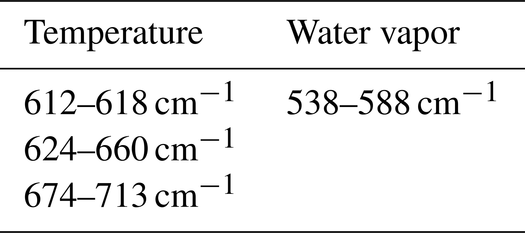
AERI has many observation channels, including not only temperature and humidity profile information, but also trace gas information such as ozone, methane, and random error. To avoid contributions to the downwelling radiance by other gases, appropriate channels that are primarily sensitive to the retrieved profiles must be selected. The spectral regions used in the study are consistent with AERIoe v1.2, which used only the 538–588 cm⁻¹ band for water vapor profiling to exclude scattering effects from clouds (Turner and Blumberg, 2019). The specific wavenumbers used to perform the retrieval are shown in Table 1, among which the spectral region used for temperature retrieval includes 167 channels and the water vapor includes 104 channels.

Table 1 Spectral regions used for retrieving temperature and water vapor profiles in the AERIoe algorithm.

2.2 Radiosonde data

Radiosondes have been used for decades to provide humidity, temperature, and wind profiles throughout the troposphere and are considered to be the most accurate means of detecting the vertical structure of the atmosphere. They are often used to evaluate the accuracy of other ground-based profilers. Located 150 m to the north of the AERI equipment, the closer radiosonde release point can ensure the comparability of radiosonde profiles and AERI retrieval results (Wakefield et al., 2021). The radiosonde data at the SGP site have been obtained by Vaisala RS92 since 2002 (Turner et al., 2016), including temperature, humidity, pressure, wind direction, and wind speed. It is regularly launched four times a day at 05:30, 11:30, 17:30, and 23:30 UTC.

We collected radiosonde profiles and AERI radiation data from 2012, screening 826 groups of qualified data samples through quality control, spatiotemporal matching, and clear-sky recognition. A synthetic dataset of simulated AERI spectra corresponding to 826 sets of radiosonde profiles was produced using the line-by-line radiative transfer model (LBLRTM), with parameter settings consistent with Sect. 3.1.

3 Methodology

3.1 Retrieval configuration

The AERIoe algorithm, based upon the optimal-estimation method, iteratively searches for the atmospheric state that most conforms to the observation and prior constraints.

$$\begin{array}{}\text{(1)}& \begin{array}{rl}{\mathit{X}}_{n+\mathrm{1}}& ={\mathit{X}}_{\mathrm{a}}+{\left({\mathbf{K}}_n^{\mathrm{T}}{\mathbf{S}}_{\mathrm{e}}^{-\mathrm{1}}{\mathbf{K}}_n+\mathit{\gamma }{\mathbf{S}}_{\mathrm{a}}^{-\mathrm{1}}\right)}^{-\mathrm{1}}{\mathbf{K}}_n^{\mathrm{T}}{\mathbf{S}}_{\mathrm{e}}^{-\mathrm{1}}\\ & \times \left({\mathit{Y}}^m-F\left({\mathit{X}}_n\right)+{\mathbf{K}}_n\left({\mathit{X}}_n-{\mathit{X}}_{\mathrm{a}}\right)\right)\end{array}\end{array}$$

Here, X is the profile of the atmospheric state to be retrieved, X_a is the prior profile of the atmosphere, S_a is the a priori covariance matrix, Y^m is the observed radiance vector, F(X) is the computed radiance for X, S_e is the observation error covariance matrix, and n denotes the iteration number. The superscripts T and −1 indicate the matrix transpose and inverse, respectively.

To improve the stability of the retrieval algorithm, the regularization parameter γ was introduced in Eq. (1), which is set as fixed values from large to small ([1000, 300, 100, 30, 10, 3, 10, 1]). As γ decreases with iterations, more observation information is introduced to improve the retrieval accuracy. Iterations are continued until γ decreases to 1 and the following convergence criterion is satisfied.

$$\begin{array}{}\text{(2)}& \mathrm{convergence}\mathrm{\_}\mathrm{index}={\displaystyle \frac{\left({\mathit{X}}_n-{\mathit{X}}_{n+\mathrm{1}}\right){\mathbf{S}}^{-\mathrm{1}}\left({\mathit{X}}_n-{\mathit{X}}_{n+\mathrm{1}}\right)}{N}}\le \mathrm{1}\end{array}$$

N represents the dimension of the retrieved atmospheric state vector.

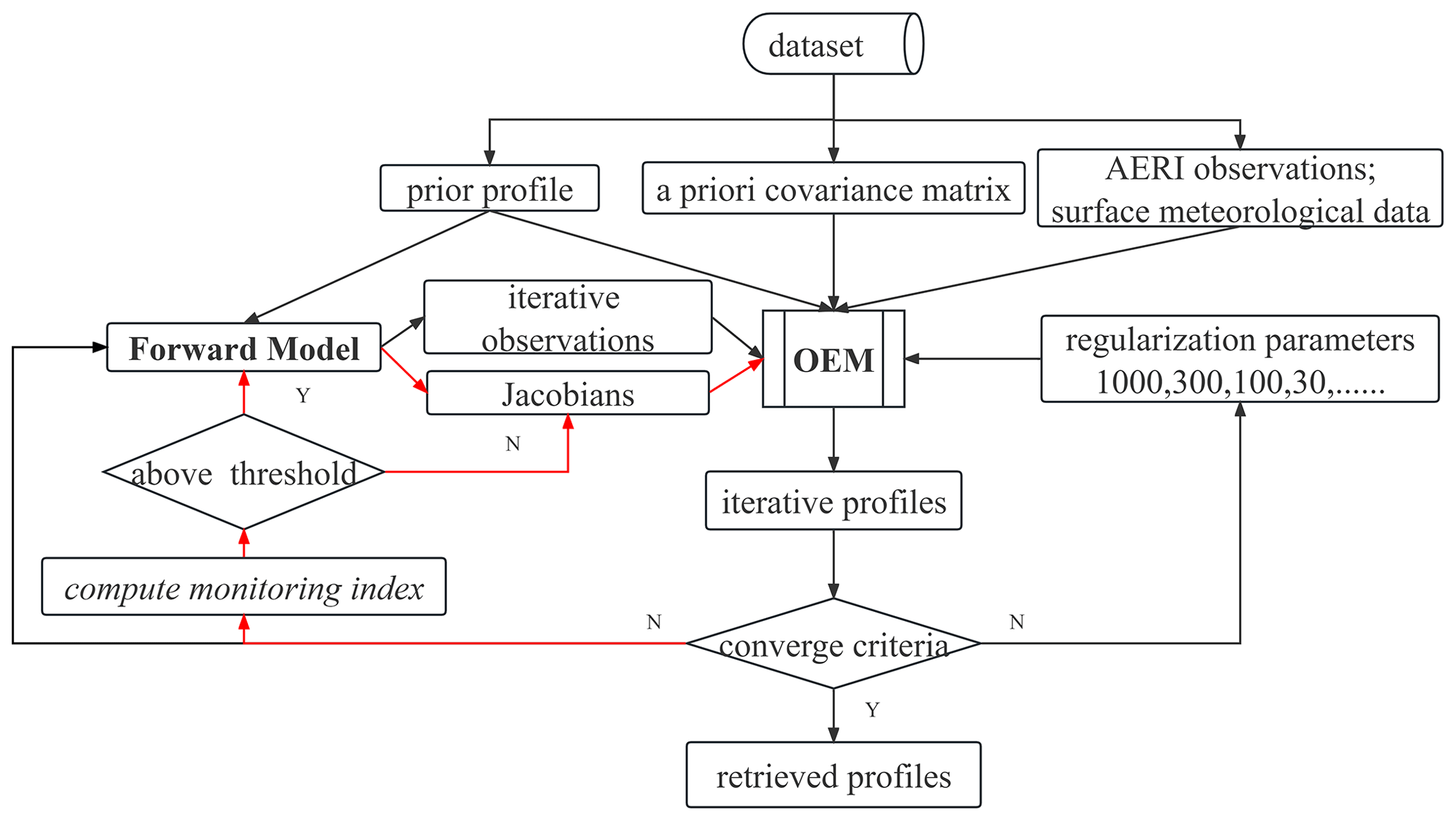
Figure 1 Flowchart of the Fast AERIoe retrieval process. Note that the red line indicates the Jacobian updating process. The iterative profiles and observations are defined as temperature and water vapor profiles at iteration n and computed radiance for X_n, respectively. The monitoring index is used to derive the variations in X_n.

Note that K depends on X used for estimating the Jacobian, which means that K must be recomputed for every iteration step. The updating of the Jacobians in the above retrieval process requires the calculation of the optical thickness or radiance (intensity) with respect to the elements of X at each height, which might be computationally expensive depending on the lengths of X and Y^m (Maahn et al., 2020). Owing to the constraints of γ, the decrease in the difference between the simulated and observed radiation is not very much in the adjustment of individual iterations to the retrieval profile. At this time, the change in the Jacobian calculated as per the iteration profile is negligible. Backed by the above analysis, a fast iterative algorithm called Fast AERIoe is proposed on the basis of the AERIoe algorithm. The flowchart of Fast AERIoe is shown in Fig. 1. Most of the configurations are consistent with AERIoe described by Turner and Löhnert (2014), except for some modifications highlighted as follows.

• a.

  Atmospheric configurations. The height grid of X is consistent with AERIoe, but the maximum retrieval height is limited to 3 km. This is done because the variations in K above 3 km are negligible because most of the information in the AERI spectrum lies in the lowest 2 km of the atmosphere for temperature and water vapor profiles (Turner and Löhnert, 2014). The cloud properties were excluded from the state vector X, which is beyond the scope of this study. The corresponding prior profile X_a and the prior covariance matrices represented by S_a are modified to be consistent with X.

• b.

  Observational vector Y. Spectral regions that are sensitive to cloud properties were removed from the observational vector Y to be consistent with the state vector X. Furthermore, additional observations, including surface temperature and water vapor, were incorporated into the observation vector; details are described by Turner and Blumberg (2019).

• c.

  Jacobian matrix K. K is derived from LBLRTM, which is the same as AERIoe except for the version (12.8 instead of 12.1). Another modification is that K is not recomputed to improve the retrieval speed of the algorithm when the variations in the iterative profile X_n are small.

3.2 Adaptive recalculation of the Jacobian

The method to reduce the calculation of K is the key to speeding up the AERIoe algorithm. The Jacobians are dependent on the atmospheric state, which means that K must be recalculated for every iteration step. The question arises as to under what circumstances K does not need to be recalculated. Therefore, the dependence of the retrieval capability on Jacobians must be analyzed, and indicators that reflect the changes in Jacobians should be determined to determine whether K is recalculated or not.

3.2.1 Quantification of algorithm retrieval capability

The retrieval accuracy of the atmospheric profile depends on the amount of atmospheric information in the hyperspectral data. Shannon information content (SIC) and degrees of freedom for signal (DFS), as important indicators to describe the effective information contained in hyperspectral data (Rodgers, 1998), can quantitatively describe the detector's retrieval ability for a specific atmospheric profile. SIC represents the reduction in uncertainty in the retrieved profiles contributed by the observation, with the calculation formula shown in Eq. (3). DFS provides the number of independent pieces of information contained in the measured radiation, with the calculation formula shown in Eq. (4).

$$\begin{array}{}\text{(3)}& {\displaystyle }\mathrm{SIC}={\displaystyle \frac{\mathrm{1}}{\mathrm{2}}}\ln \det \left({\widehat{\mathbf{S}}}^{-\mathrm{1}}{\mathbf{S}}_{\mathrm{a}}\right)\text{(4)}& {\displaystyle }\mathrm{DFS}=\mathrm{Trace}\left({\mathbf{B}}^{-\mathrm{1}}{\mathbf{K}}_n^{\mathrm{T}}{\mathbf{S}}_{\mathrm{e}}^{-\mathrm{1}}{\mathbf{K}}_n\right)\end{array}$$

Here, $\widehat{\mathbf{S}}$ is the posterior error covariance matrix, also known as the analysis error covariance matrix. Its diagonal element is the standard deviation of the retrieval error, with the calculation formula $\widehat{\mathbf{S}}$ as follows:

$$\begin{array}{}\text{(5)}& \widehat{\mathbf{S}}={\mathbf{B}}^{-\mathrm{1}}\left({\mathbf{K}}^{\mathrm{T}}{\mathbf{S}}_{\mathrm{e}}^{-\mathrm{1}}\mathbf{K}+{\mathit{\gamma }}^{\mathrm{2}}{\mathbf{S}}_{\mathrm{a}}^{-\mathrm{1}}\right){\mathbf{B}}^{-\mathrm{1}},\end{array}$$

of which

$$\begin{array}{}\text{(6)}& \mathbf{B}=\left(\mathit{\gamma }{\mathbf{S}}_{\mathrm{a}}^{-\mathrm{1}}+{\mathbf{K}}_n^{\mathrm{T}}{\mathbf{S}}_{\mathrm{e}}^{-\mathrm{1}}{\mathbf{K}}_n\right).\end{array}$$

3.2.2 Analysis of the dependence of AERIoe on Jacobians

It can be seen from Eqs. (3) and (4) that SIC and DFS are determined by S_e, S_a, K, and γ. However, S_a and S_e remain unchanged during retrieval, which makes SIC and DFS change with iteration due to variations in γ and K. As γ drops to 1 at the final iteration, the values of SIC and DFS are only dependent on K. Owing to the difficulty in quantifying the change in the two-dimensional Jacobian caused by the iteration profiles, a monitoring index, henceforth called K_Index, is designed and used to characterize the change in the profiles at various iterations. The calculation of K_Index comes from the convergence criterion convergence_index, which contains not only the difference between the iteration profiles, but also the posterior dominated by the Jacobian. The introduced K_Index should reflect the changes in the temperature and humidity profiles, which means that the influence of the Jacobian should be excluded. Then, the convergence_index was degenerated into the K_Index as follows.

$$\begin{array}{}\text{(7)}& \mathrm{K}\mathrm{\_}\mathrm{Index}={\displaystyle \frac{{\left({\mathit{X}}_n-{\mathit{X}}_{n+\mathrm{1}}\right)}^{\mathrm{T}}\left({\mathit{X}}_n-{\mathit{X}}_{n+\mathrm{1}}\right)}{N}}\end{array}$$

The values of K_Index in Fig. 2, which cover most of the K_Index during the AERIoe retrieval process (ranging from 0 to 260; see Fig. 3), were obtained by multiplying the prior profile by different scale factors. The atmosphere-dependent K values were computed by the LBLRTM with the prior profiles above, and SIC and DFS were calculated using Eqs. (3) and (4), respectively, with different Jacobians. Both SIC and DFS change slowly with K_Index as shown in Fig. 2, with the variation of SIC within 13 % (from 13.9 to 16.1) and that of DFS within 4 % (from 3.7 to 3.9) for temperature and 13 % (from 1.4 to 1.7) for water vapor, which demonstrates that SIC and DFS remain almost unchanged on the condition that the value of K_Index is small. This provides an effective means of improving the retrieval speed of AERIoe by recalculating K selectively when X is not changing much or K_Index is small. This could be achieved by comparing the value of K_Index with its threshold at each iteration to determine whether K is recalculated or not.

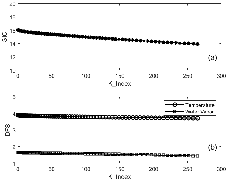
Figure 2 (a) The change in SIC as a function of K_Index. (b) The change in DFS as a function of K_Index for temperature (unfilled circles) and water vapor (open squares).

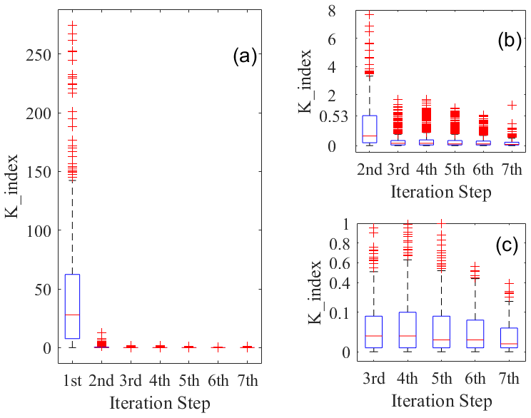
Figure 3 Box-and-whisker plots for K_Index values at different iterations in the retrieval process of AERIoe. (a) K_Index values calculated using 826 samples at iterations 1–7. Panels (b) and (c) are the same as panel (a) but for iterations 2–7 and iterations 3–7, respectively. The boxes show upper-quartile, median (the red line through the middle of the box), and lower-quartile values for K_Index. The whiskers extend to 1.5 times the interquartile range (IQR). Any outliers above or below the whiskers are plotted as red symbols “+”.

3.2.3 Determination of the K_Index threshold

The selection of the threshold for K_Index is very important for the Fast AERIoe algorithm. If the threshold remains too large, too many Jacobians will stop updating, resulting in a decline in retrieval accuracy or even nonconvergence of the retrieval process; when the threshold value remains too small, most Jacobians need to be recalculated, which cannot effectively shorten the retrieval time.

Figure 3 shows the histogram of the K_Index distribution for each iteration in the retrieval process, with the K_Index values at each iteration calculated using the clear-sky data for 2012. Since the climatological mean profile was used as the first guess, which has a large deviation from the real atmospheric state, a larger value of K_Index was demonstrated in the first step of the retrieval. The K_Index value decreases significantly from the second iteration (see Fig. 3a), indicating that the adjustment of the iterative profile remains very small and that the retrieval process tends to be stable relative to the first iteration. As the retrieval proceeds, the iteration profile gradually approaches the truth, and the K_Index box gradually shortens to below 0.5 (see Fig. 3b). Using this value as the threshold for K_Index, most of the Jacobian after the second iteration does not need to be recalculated, and the retrieval time could be effectively reduced. However, the K_Index in iteration 7 shows larger outliers, indicating that the instability of the retrieval algorithm increases when the γ factor decreases to 1. To reduce the impact of the Jacobian on the convergence of the algorithm, the threshold for the K_Index after iteration 6 is set to 0.1 according to Fig. 3c, of which the K_Index box at iteration 7 is within 0.1. It should be noted that the threshold of K_Index used in the Fast AERIoe algorithm is dependent on the datasets used in the retrieval. They are presented “as is” and are not intended to be directly applied by the reader. We encourage readers to develop their own indicator to reduce the recalculation of Jacobians based on the atmospheric profiles they intend to retrieve.

4 Results and discussions

The simulated AERI radiation is used for retrieval to better analyze the performance of Fast AERIoe and to eliminate the interference of other factors. An advantage of using synthetic observations is that the true atmospheric state is known, which can be used to evaluate the retrieval accuracy. Second, the errors caused by parameters in the forward model, such as the deviation of trace gas content, the strength and temperature dependence of the water vapor continuum absorption, and the half-widths of absorption lines, could be eliminated (Maahn et al., 2020). Third, we can control the noise level in the synthetic measurement.

4.1 Retrieval process

Examples of the Fast AERIoe retrieval using the simulated spectra at various iterations are shown in Fig. 4. These profiles represent the typical performance of each retrieval configuration at the SGP site. The entire retrieval process took 3.59 min with seven iterations, in which only Jacobians of the first and second iterations were updated. The retrieved profiles converged quickly below 1 km, with little adjustment of the temperature and humidity profiles following the first iteration. For the upper atmosphere above 1.5 km, the temperature and humidity profiles have a relatively large adjustment and gradually approach the radiosonde profile with the iterations. This feature of the Fast AERIoe retrieval process is very similar to AERIoe, which is determined by the information content of the AERI spectra. The information content is concentrated near the surface, which leads to a more rapid convergence in the lowest portions of the profile. The information content of the upper layer is lower, and as such it is necessary to reduce the value of γ to introduce more observation information so that the retrieved profiles are refined to approach the radiosonde profile as the iterations are continued.

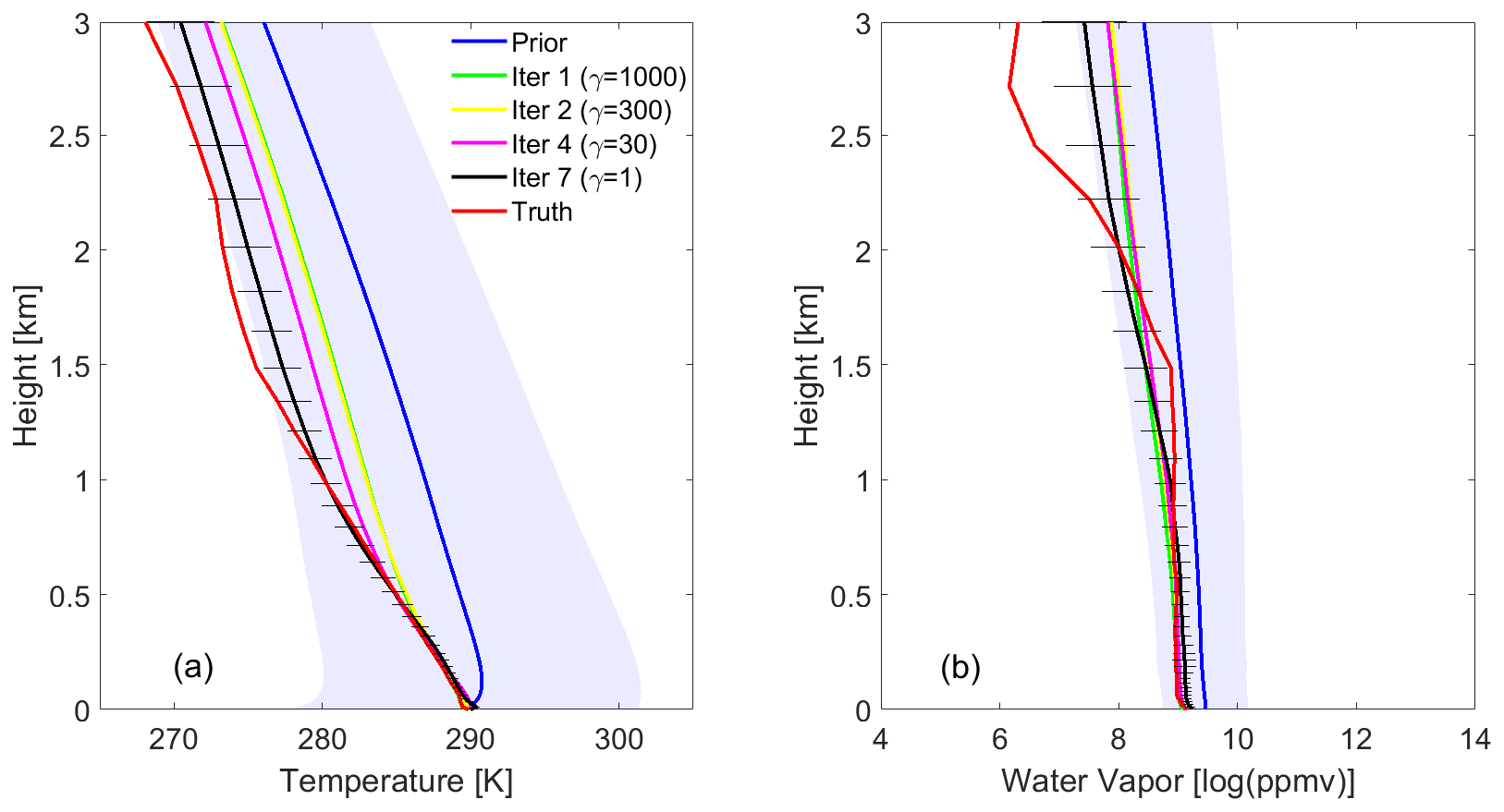
Figure 4 Retrieved (a) temperature and (b) water vapor profiles at various iterations from the simulated AERI observations, where the simulated observations were computed from a radiosonde (shown in red curves) launched at the SGP site at 11:30 UTC on 20 April 2012. The prior mean profile (blue) was used as the first guess, and the blue-shaded area illustrates the 1σ uncertainties in the prior. The profiles at iterations 1, 2, and 7 are shown in solid blue, yellow, purple, and black (with 1σ error bars derived from $\widehat{\mathbf{S}}$) lines, and the γ values were set to 1000, 300, 30, and 1, respectively, for the above iterations.

One advantage of the optimal-estimation method remains that the posterior error covariance matrix of the solution $\widehat{\mathbf{S}}$ can be obtained to estimate the uncertainty of the retrieval results of each sample. The temperature and water vapor profiles show a strong correlation for the correlation coefficient matrix of S_a (see Fig. 5a and c), especially the temperature profile, which has a high correlation coefficient above 0.6 between any two layers because of the relatively stable vertical gradient of the temperature profile. The nondiagonal elements below 1 km in the correlation coefficient matrix of the $\widehat{\mathbf{S}}$ results from Fast AERIoe show a much lower correlation than those of S_a (see Fig. 5b and d), which means that the retrieved profiles in the lower atmosphere are dominated by AERI observations. However, with increasing height, the correlation of the area near the diagonal increases significantly. Therefore, the retrieval algorithm will rely more on the constraint of prior information at the upper layer of the PBL. The 1σ uncertainty lines, which are the square root of the diagonal of the covariance matrices for the prior (blue-shaded area) and the posterior (black horizontal line) in Fig. 4, demonstrate that the retrieved profile has a much smaller uncertainty than the prior. Therefore, the Fast AERIoe algorithm can effectively reduce the impact of uncertainties in the first-guess profile on the retrieval results. As the height increases, the black horizontal line segment becomes longer for either the temperature profile or the water vapor profile, indicating that the uncertainty in the retrieved profiles increases in the upper PBL.

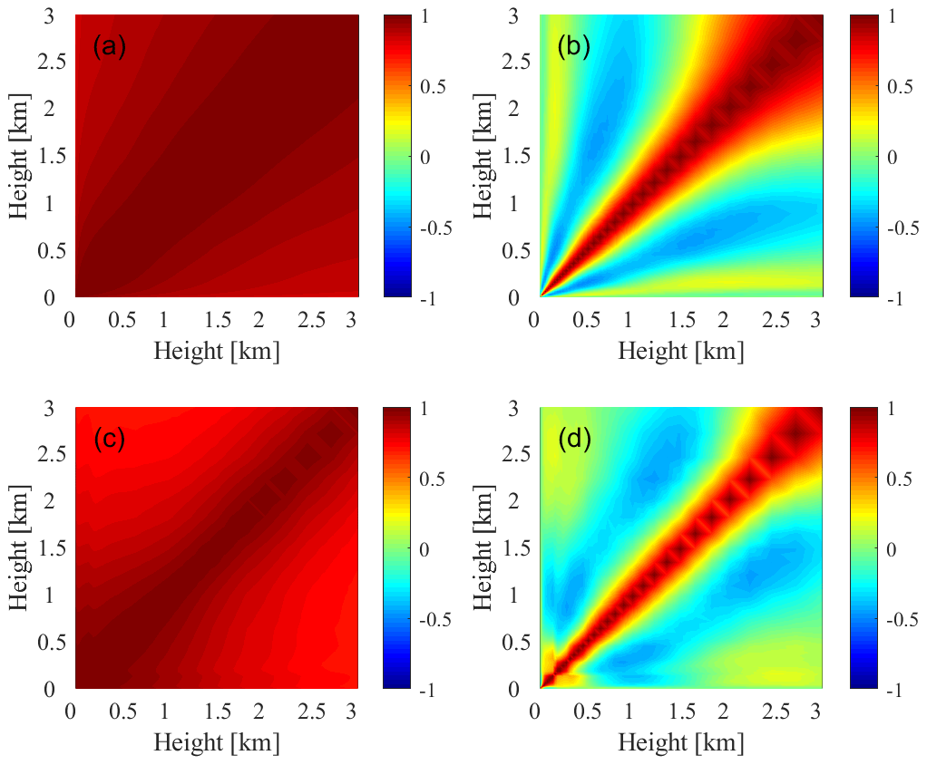
Figure 5 The level-to-level correlation of the prior (a, c) and posterior (b, d) for temperature (a, b) and water vapor (c, d) at 11:30 UTC on 20 April 2012.

4.2 Performance

4.2.1 Retrieval time

Both the AERIoe and Fast AERIoe algorithms were used to retrieve 826 groups of simulated AERI radiation data at SGP stations in 2012 to evaluate the retrieval performance of Fast AERIoe. The codes for both of the retrieval algorithms are written in the MATLAB language and run on a Lenovo Aircross 510P computer, of which the CPU is Intel Core i7-7700 and the operating system is Ubuntu 14.04. To analyze the code timing of the retrieval algorithm, the code was divided into the following sections: preparation, iteration 1, iteration 2, and iteration 3, etc., until the final iteration. The preparation section mainly consists of atmosphere construction, observation vector construction, and precalculated variable importation. The iteration sections include the recalculation of K and F(X) and the inversion using Eq. (1). Note that iteration 1 does not need to calculate K and F(X) because the prior profile X_a is fixed (mean value of the atmosphere), and the K and F(X) associated with it are precalculated. The time consumed by each section was analyzed for both AERIoe and Fast AERIoe, and the results for an arbitrarily selected case are provided in Table 2. The recalculation of F(X) and K consumed an immense amount of time in the retrieval process of AERIoe, and the latter is the most time-consuming section. Therefore, by reducing the recalculation of K, the retrieval time of Fast AERIoe is greatly reduced compared to AERIoe.

Table 2 List of time consumption (unit: s) by the AERIoe and Fast AERIoe sections. The sections denoted with superscript “^∗” indicate that K is not recalculated during the Fast AERIoe retrieval process.

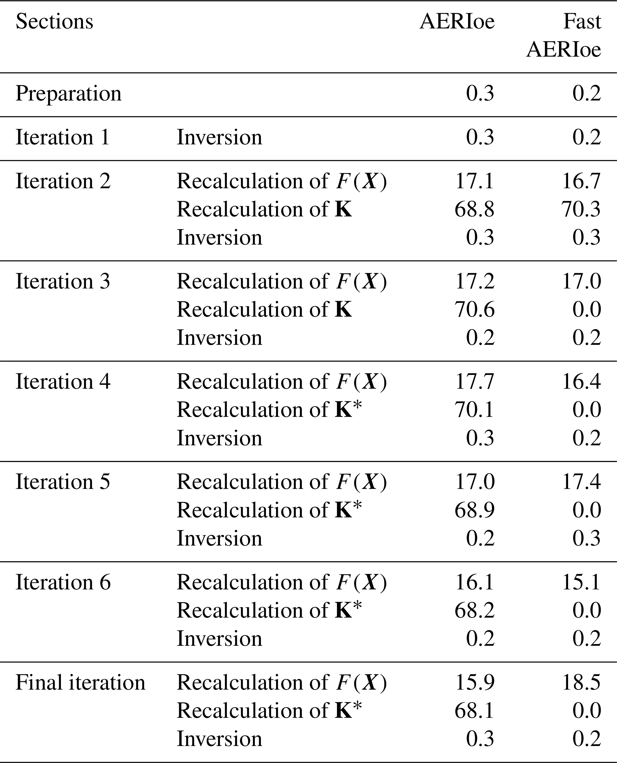
The average retrieval time of Fast AERIoe for the 826 cases used in the study is 3.7 min, which is more than 50 % shorter than that of AERIoe, with an average retrieval time of 9.0 min, which is beyond the temporal resolution (approximately 8 min) of AERI observations. All of the AERIoe samples consumed more than 8 min, while only 10 cases exceeded the temporal resolution of AERI for the Fast AERIoe algorithm. Note that the retrieval time is dependent on the computing platform and the method used to compute Jacobians and is not intended to be directly applied by the reader.

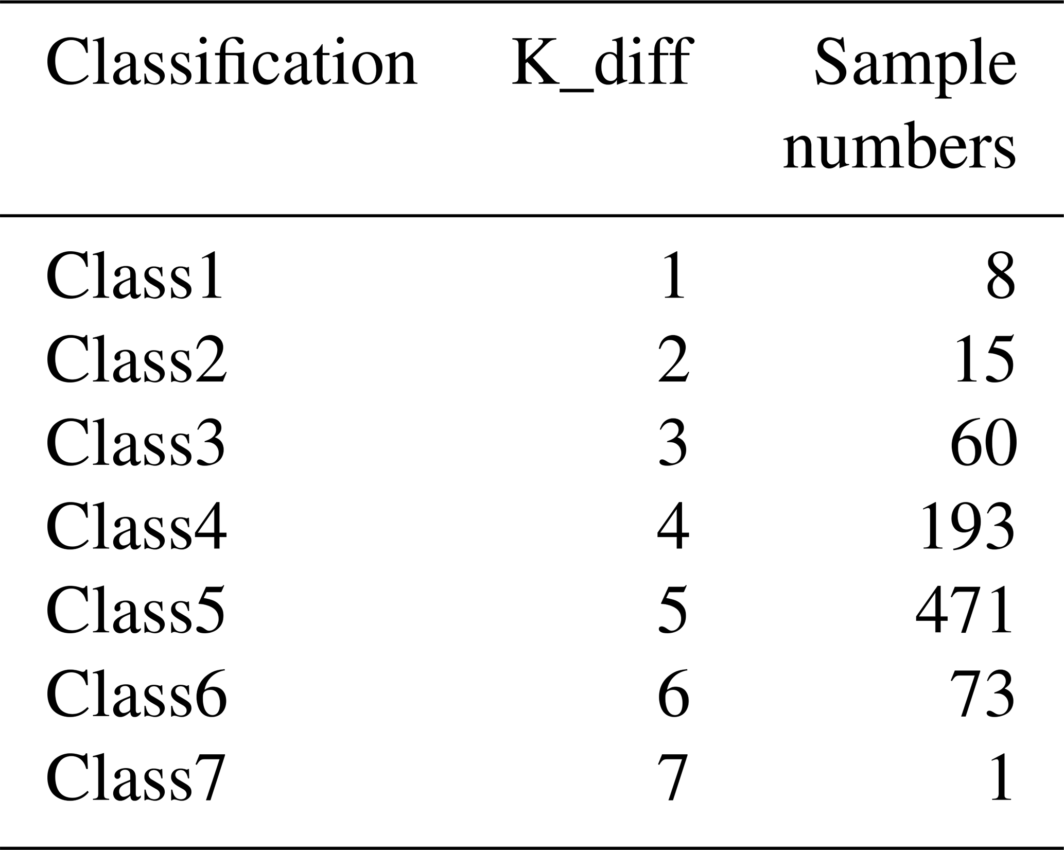
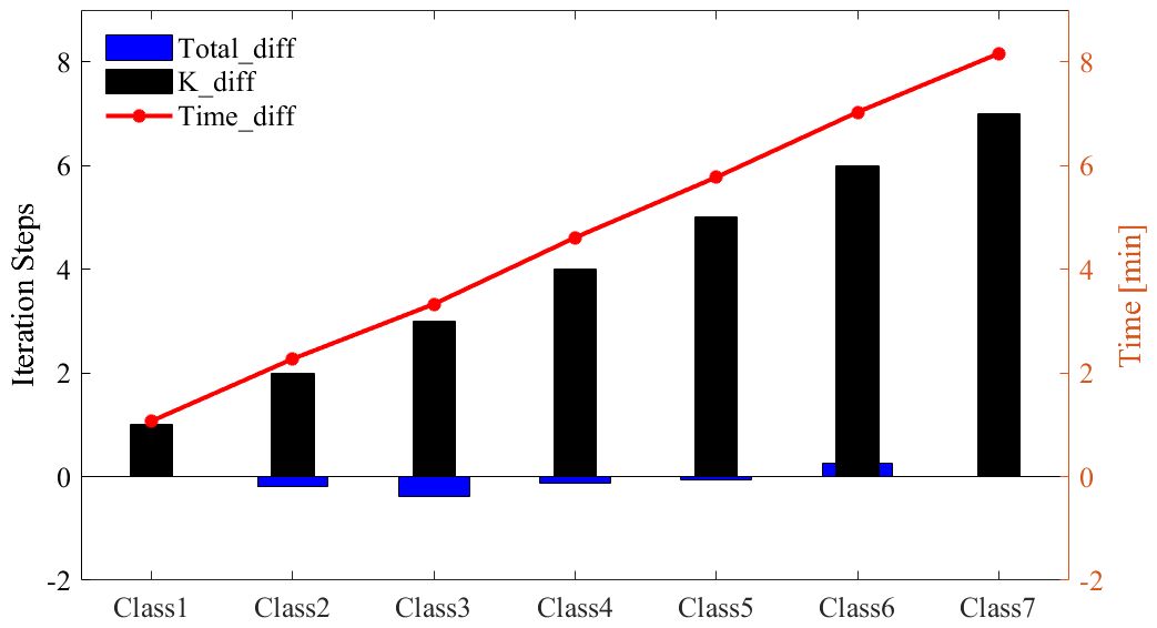
In addition to the recalculation of K, the retrieval time is also affected by the total iteration steps. Therefore, statistics of the average retrieval time difference (Time_diff for short) caused by the K recalculation step difference (K_diff for short) and the average total iteration step difference (Total_diff for short) are provided in this study. The retrieval samples are divided into seven categories (shown in Table 3), in keeping with K_diff between AERIoe and Fast AERIoe. On this basis, Time_diff and Total_diff between the two retrieval algorithms for various samples are calculated. As shown in Fig. 6, with an increase in K_diff, Time_diff also increased gradually, showing a strong positive correlation. Compared with K_diff, the value of Total_diff is very small, and its impact on the retrieval time is also minimal, only having slight negative and positive effects on the Time_diff of Class3 and Class6. Therefore, the improvement in the retrieval speed of Fast AERIoe is mainly due to the recalculation of Jacobians.

Table 3 The number of samples of different classes, which are classified according to K_diff.

Figure 6 The distribution of K_diff, Total_diff, and Time_diff with different classes.

4.2.2 Convergence characteristics

A total of 825 samples of the 826 datasets using the AERIoe algorithm achieved convergence, with the convergence rate reaching 99.9 %. The Fast AERIoe algorithm has 815 groups of samples to achieve convergence, with the convergence rate reaching 98.7 %, which is lower than that of AERIoe. Among the 11 sets of retrieval samples that did not achieve convergence, the K_Index of most of them did not change much after the γ was dropped to 1, indicating that the subsequent iterations had little effect on the adjustment of the profiles, so the iterative profile corresponding to the minimum convergence_index could be taken as the retrieval results instead of criterion (2). Figure 7a shows the comparison between the retrieved profiles from AERIoe using criterion (2) and Fast AERIoe using the new convergence criteria with 11 sets of nonconverged samples. The temperature profiles obtained by the two algorithms are virtually identical, with an R² of 0.99. For the water vapor mixing ratio (WVMR), the introduction of the new convergence criteria reduces the value of R², but this still reaches 0.84, indicating that the two datasets still have a strong correlation. The above results indicate that the method of using the minimum convergence_index to obtain the retrieval profiles is a reasonable and feasible method, as the Fast AERIoe algorithm cannot achieve convergence.

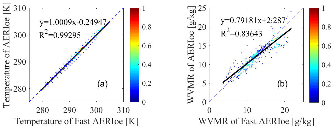
Figure 7 Scatter plots between the retrieval results of the nonconverged samples with AERIoe and Fast AERIoe. (a) Temperature profiles. (b) WVMR profiles.

4.2.3 Accuracy

Traditional methods used to evaluate the accuracy of retrieved profiles against radiosondes compute the BIAS and root-mean-square error (RMSE), with the calculation formula as follows:

$$\begin{array}{}\text{(8)}& {\displaystyle }\mathrm{BIAS}\left(i\right)={\displaystyle \frac{\sum _{j=\mathrm{1}}^M\left({\mathit{X}}_{\mathrm{sonde}}^{\mathrm{smooth}}(i,j)-{\mathit{X}}_{\mathrm{retrieval}}(i,j)\right)}{M}},\text{(9)}& {\displaystyle }\mathrm{RMSE}\left(i\right)=\sqrt{{\displaystyle \frac{\sum _{j=\mathrm{1}}^M{\left({\mathit{X}}_{\mathrm{sonde}}^{\mathrm{smooth}}(i,j)-{\mathit{X}}_{\mathrm{retrieval}}(i,j)\right)}^{\mathrm{2}}}{M}}},\end{array}$$

where i and j represent the serial numbers of vertical stratification and samples, respectively, with M being the number of samples. X_retrieval is defined as retrieved profiles, and ${\mathit{X}}_{\mathrm{sonde}}^{\mathrm{smooth}}$ is radiosonde observations that are smoothed with the averaging kernel A by the following multiplication to reduce the vertical representativeness errors:

$$\begin{array}{}\text{(10)}& {\mathit{X}}_{\mathrm{sonde}}^{\mathrm{smoothed}}=\mathbf{A}\left({\mathit{X}}_{\mathrm{sonde}}-{\mathit{X}}_{\mathrm{a}}\right)+{\mathit{X}}_{\mathrm{a}}.\end{array}$$

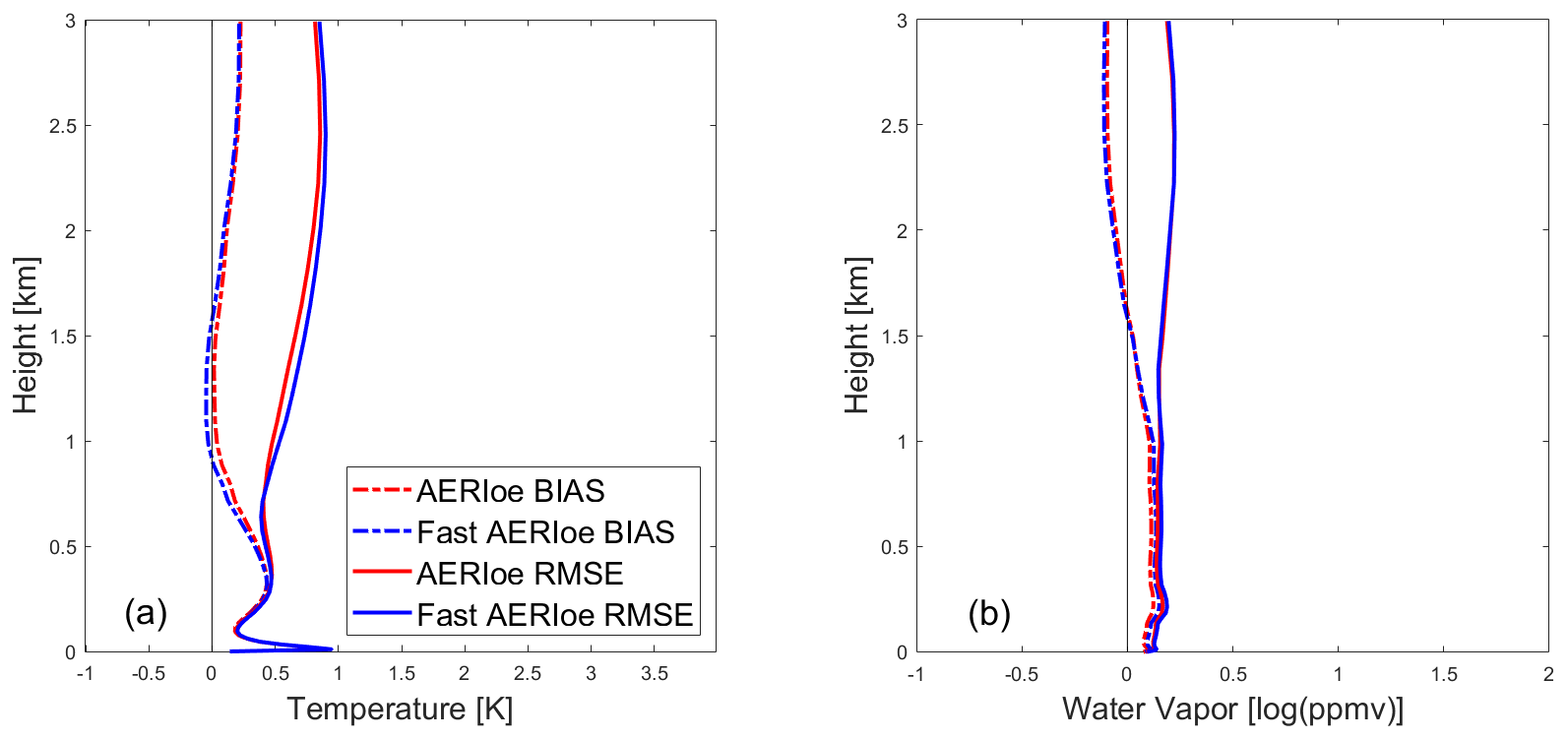
Figure 8 Bias (solid curves) and RMSE (dashed curves) profiles for clear-sky comparisons of the AERIoe (red curves) and Fast AERIoe (blue curves) retrievals with radiosondes. (a) Temperature profiles. (b) Water vapor profiles.

The BIAS and RMSE of AERIoe and Fast AERIoe are calculated for 826 sets of samples using the above equations within the altitude range of 0–3 km, and the results are shown in Fig. 8. The temperature profile below 1.0 km and the water vapor profile below 1.5 km have obvious positive deviations, with the maximum deviations reaching 1.0 K and 0.2 log(ppmv), respectively. However, the BIAS and RMSE at the bottom are significantly reduced due to the constraint of the surface observations, indicating that the introduction of surface meteorological observation data into the observation vector has an obvious positive effect. The temperature profiles retrieved by Fast AERIoe show a negative deviation of 0.05 K between 1.0 and 1.5 km and a maximum increase in RMSE within 0.08 K above 1.0 km when compared with AERIoe. For the water vapor profile, the BIAS and RMSE profiles of Fast AERIoe are in good agreement with AERIoe, except for a maximum increase in BIAS within 0.03 log(ppmv) below 1.0 km. When considering the magnitude of the temperature (roughly on the order of 300 K) and water vapor (roughly on the order of 5–10 log(ppmv)) profiles, the differences between the retrieved profiles are negligible, indicating that the retrieval results of Fast AERIoe are comparable to those of AERIoe.

The comparison of the profiles retrieved by the two algorithms can be demonstrated more clearly by the modified Taylor plots (Turner and Löhnert, 2014), which are used to evaluate how well each retrieved profile can capture the vertical shapes of its true profile, as BIAS and RMSE can only describe the average accuracy of the whole dataset at each height. These Taylor diagrams show Pearson's correlation coefficient between two datasets on the y axis and the ratio of the standard deviation on the x axis. Each retrieval–sonde pair is used to derive the correlation coefficient (r) from Eq. (11) and the ratio of the standard deviations from Eq. (12); both are used by Turner and Löhnert (2014).

$$\begin{array}{}\text{(11)}& {\displaystyle }r={\displaystyle \frac{\frac{\mathrm{1}}{N}\sum _{z=\mathrm{0}}^{z=h}\left[s\left(z\right)-\stackrel{\mathrm{‾}}{s}\right]\left[a\left(z\right)-\stackrel{\mathrm{‾}}{a}\right]}{{\mathit{\sigma }}_{\mathrm{s}}{\mathit{\sigma }}_{\mathrm{a}}}},\text{(12)}& {\displaystyle }\mathrm{SDR}={\mathit{\sigma }}_{\mathrm{a}}/{\mathit{\sigma }}_{\mathrm{s}}.\end{array}$$

Within the equations, s(z) and a(z) are defined as the radiosonde observations and retrieved profiles between 0 and 3 km, and ($\stackrel{\mathrm{‾}}{s},\stackrel{\mathrm{‾}}{a}$t) and (σ_s,σ_a) are the mean values and standard deviations in the same height range.

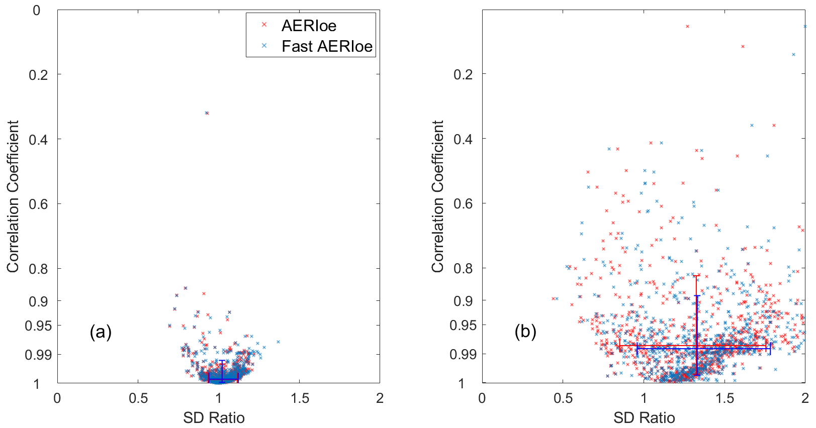
Figure 9 Modified Taylor plots showing the correlation coefficient and standard deviation ratio between the smoothed radiosondes and the retrieved clear-sky (a) temperature and (b) water vapor using AERIoe (red symbols) and Fast AERIoe (blue symbols). There were 826 cases from the SGP site within 2012. Each symbol indicates the score for an individual profile. The arms of the plotted crosses span the 10th–90th percentiles for the correlation coefficient (vertical arms) and the standard deviation ratio (horizontal arms).

Retrievals that have a correlation coefficient of 1 and a standard deviation ratio (SDR) of 1 mean that the two datasets match perfectly. Figure 9a and b show these plots for the clear-sky AERIoe and Fast AERIoe retrievals. For the temperature retrievals, both Fast AERIoe and AERIoe perform well, with 90 % of the correlation coefficients above 0.9 and the intersection of the arms close to 1. Figure 9b shows that retrieving the water vapor structure is much more difficult with both algorithms; the spreads in the correlation coefficient and SDR are much larger for water vapor than for temperature. Most of the blue and red symbols “×” in Fig. 9, which indicate the scores for the individual profiles of the two algorithms, are close to each other for both the temperature and water vapor profiles. Therefore, the modified Taylor plots also confirm the conclusion that the retrieval results of the AERIoe and Fast AERIoe algorithms are comparable.

4.3 Real observations

Since the clouds overhead have a significant influence on the infrared spectra, the primary problem is how to screen clear-sky samples when using the measured AERI data to retrieve the temperature and humidity profiles. The contribution of clouds to infrared radiation not only interferes with the inversion of temperature and humidity profiles, but also provides technical means for obtaining cloud macrophysical properties (Liu et al., 2022). Figure 10 shows the AERI-observed spectrum under cloudy- and clear-sky conditions. The AERI observations under the two conditions remain highly different, indicating that the AERI-observed spectrum can be adopted directly to determine whether clouds or clear skies are present. To establish an accurate cloud recognition model, we adopted the cloud fraction data obtained from the all-sky image at the same site as the label for training, where the sample with a cloud fraction of less than 30 % is marked as 0, indicating clear sky, while the sample with a cloud fraction greater than 30 % is marked as 1, indicating that there is cloud overhead. Using the abovementioned method, the cloud fraction of the all-sky image from March to May 2010 was labeled and temporally matched with the AERI-observed radiance to form a training dataset, based on which a cloud recognition model was established by training the back-propagation (BP) neural network, with the final cross-validation accuracy reaching 94.3 %. Compared with the recognition method by radiosonde, the BP cloud recognition model greatly improves the discrimination accuracy without requiring additional detection equipment. The BP cloud recognition model was applied to the 178 groups of AERI observations collected on 21 October 2012, with 168 groups of clear-sky samples screened in total.

Figure 10 AERI observations in clear- and cloudy-sky conditions.

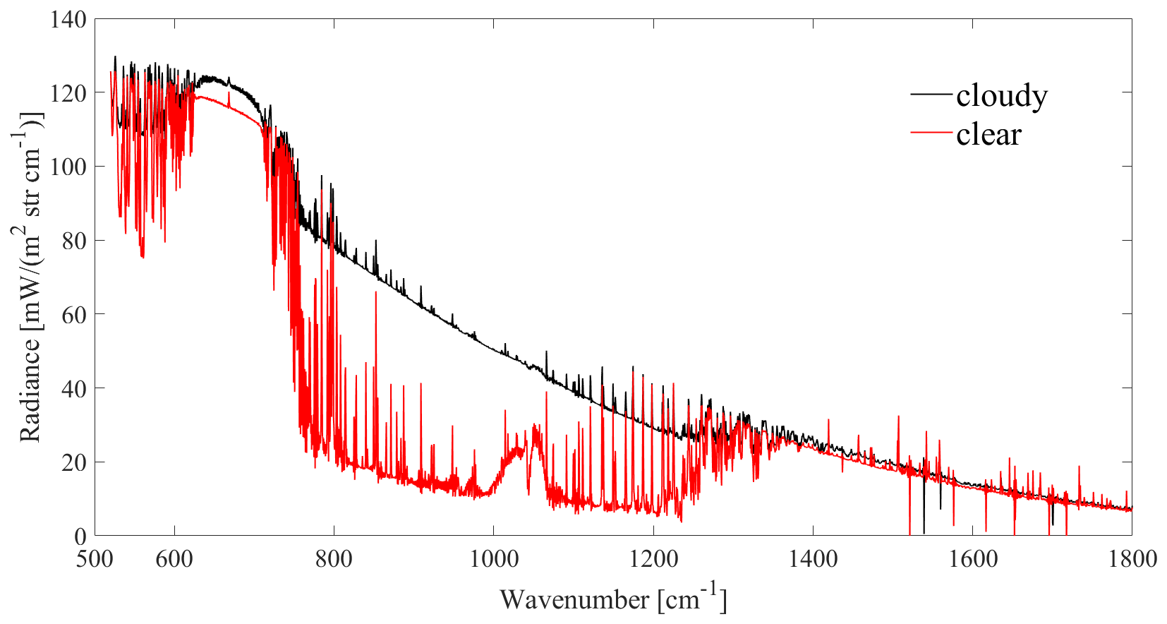
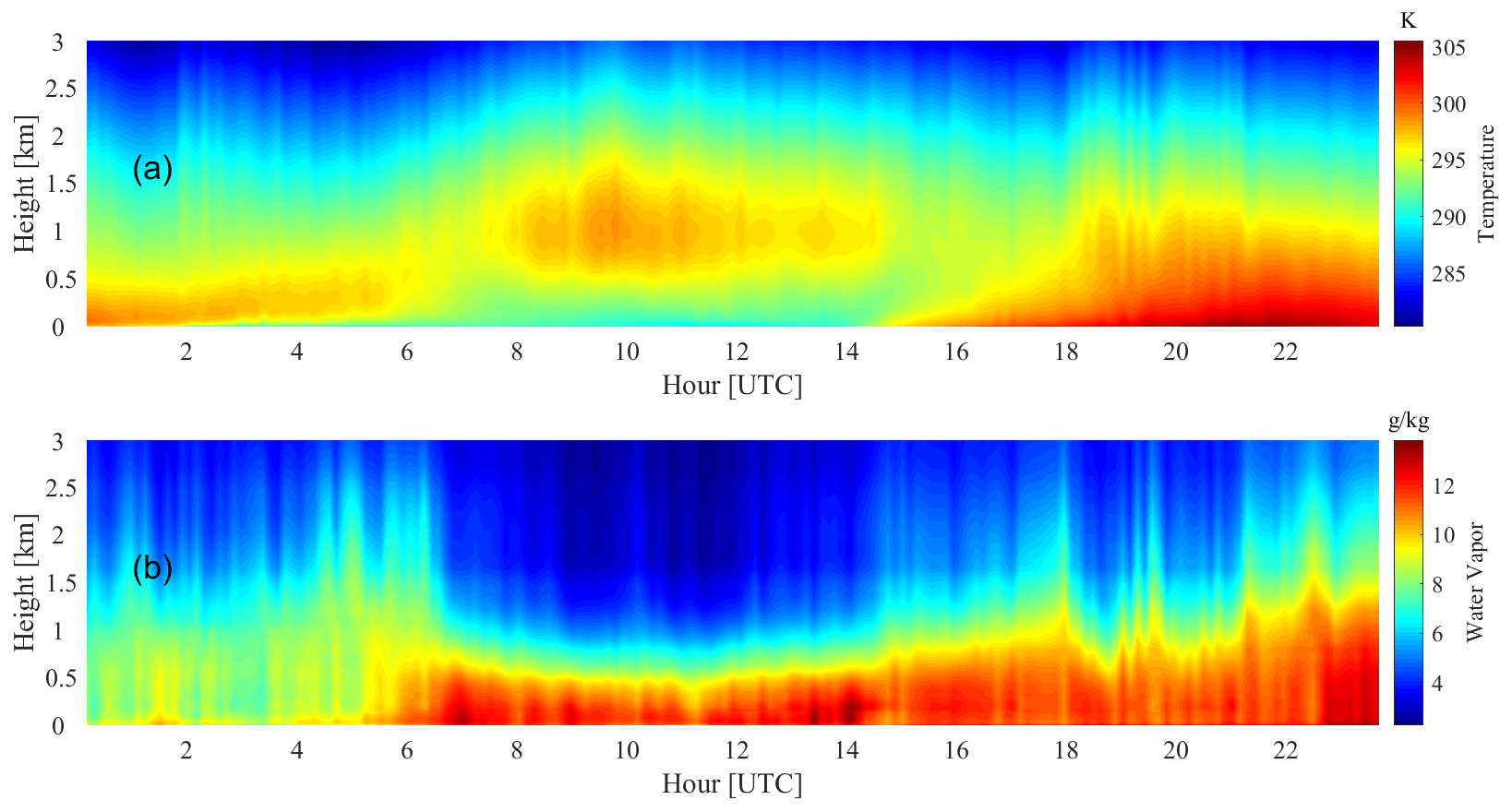
Figure 11 Time–height cross sections of temperature (a) and water vapor (b) on 21 October 2012.

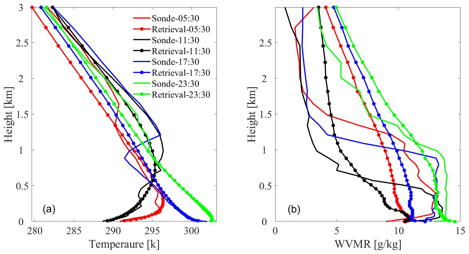
Figure 12 Comparisons between retrieved thermodynamic profiles and the coincident radiosonde profiles at 05:30, 11:30, 17:30, and 23:30 UTC on 21 October 2012. (a) Temperature profiles. (b) WVMR profiles.

Benefitting from good retrieval accuracy and high temporal resolution, AERI instruments can be used to monitor thermodynamic temporal structures that may not be resolved by infrequent radiosonde launches. Figure 11 shows the time–height cross sections of the temperature and WVMR profiles derived from the Fast AERIoe retrievals. Figure 11 shows that AERI resolved the temperature inversion prior to approximately 15:00 UTC, and the height of the inversion layer gradually increased over time. After 15:00 UTC, the temperature near the surface increases significantly, accompanied by the disappearance of the inversion layer. From the comparisons with radiosonde profiles shown in Fig. 12, the retrieval results of Fast AERIoe are well matched with radiosonde profiles, especially the temperature profiles, which demonstrates the ability of the algorithm to resolve the inversion layer.

5 Conclusions

The AERIoe algorithm retrieves atmospheric temperature and humidity profiles using the optimal-estimation framework, which can make full use of information in the infrared spectrum and give the uncertainty of each retrieval result. AERIoe reduces the dependence on the first-guess profile by introducing regularization parameters, but it also requires more iterative steps, which increases the calculation amount and retrieval time of the algorithm. In this paper, a fast-retrieval method called Fast AERIoe was established by adaptively recalculating the Jacobians in the retrieval process of AERIoe. Based on the statistical comparison of the two methods (AERIoe and Fast AERIoe) with radiosonde observations, the retrieval performance of Fast AERIoe is summarized as follows.

1. The retrieval speed of Fast AERIoe is significantly improved compared with AERIoe while keeping the parameters of the computing platform unchanged, with the average retrieval time reduced by more than 50 %. The temperature and water vapor profiles derived from Fast AERIoe are almost unchanged compared with AERIoe, illustrating that the retrieval results of Fast AERIoe are comparable to those of AERIoe. The deep retrieval architecture is able to extract highly nonlinear features from the AERI observations and shows a better inversion capability than the existing statistical methods (Yang et al., 2023), albeit with the lack of the radiative transfer process. Therefore, the combination of AERIoe and deep learning can improve the accuracy of AERI for retrieving temperature and humidity profiles.

2. For the convergence characteristics, 825 out of 826 samples adopting AERIoe meet the convergence criterion, while the sample adopting Fast AERIoe converges over 98 % of the time. The method of recalculating Jacobians in Fast AERIoe slightly reduces the convergence of the retrieval algorithm. Despite this, the Fast AERIoe algorithm has demonstrated the ability to retrieve reliable temperature and water vapor profiles more quickly, which is fast enough for real-time processing.

3. When Fast AERIoe is adopted to measure the AERI spectrum, a cloud recognition model without additional detection equipment is established based on the BP neural network algorithm to remove cloudy-sky cases. Compared with the commonly used cloud recognition method by radiosonde observations, the BP cloud recognition model has greatly improved the discrimination accuracy. It should be noted that the hyperspectra under the two weather conditions of clear sky with high humidity and few clouds are relatively close, while the above two weather conditions are far from further distinguished when building the BP cloud recognition model, which may reduce the discriminative accuracy of the model. Furthermore, the cloud base height (CBH) also contributes to AERI radiation (Ye et al., 2022), and adding CBH to the recognition model helps to improve the accuracy of the model.

A single instrument always has some defects in vertical coverage, vertical resolution, temporal resolution, and accuracy in obtaining the vertical distribution of atmospheric continents (Barrera-Verdejo et al., 2016). The combination of multiple remote-sensing devices in an optimal retrieval algorithm can overcome the shortcomings of a single device, making full use of each measurement to achieve the purpose of enhancing their benefits. However, the increase in observation equipment will inevitably lead to more complex calculations of the forward model and Jacobian, which will lead to a significant increase in the amount of calculation and retrieval time. Therefore, it is particularly necessary to carry out research on fast retrieval in the case of joint retrieval. Apart from the influence of the Jacobian on the retrieval time, so is the number of iterations required by the retrieval algorithm, which is dominated by the regularization parameter. Future work will focus on the application of Fast AERIoe in the combination of different observations and the selection of regularization parameters to permit the retrieval algorithm to converge more efficiently.