Challenges and solutions in determining dilution ratios and emission factors from chase measurements of passenger vehicles

Vehicle chase measurements used for studying real-world emissions apply various methods for calculating emission factors. Currently available methods are typically based on the dilution of emitted carbon dioxide (CO₂) and the assumption that other emitted pollutants dilute similarly. A problem with the current methods arises when the studied vehicle is not producing CO₂, e.g. during engine-motoring events, such as on downhill sections. This problem is also encountered when studying non-exhaust particulate emissions, e.g. from electric vehicles. In this study, we compare multiple methods previously applied for determining the dilution ratios. Additionally, we present a method applying multivariate adaptive regression splines and a new method called near-wake dilution. We show that emission factors for particulate emissions calculated with both methods are in line with the current methods for vehicles producing CO₂. In downhill sections, the new methods were more robust to low CO₂ concentrations than some of the current methods. The methods introduced in this study can hence be applied in chase measurements with changing driving conditions and be possibly extended to estimate non-exhaust emissions in the future.

1 Introduction

Anthropogenically emitted gaseous compounds and particulate matter have effects on both climate and human health (Forster et al., 2021; Lelieveld et al., 2015). Vehicle emissions contribute to a significant proportion of those emissions, especially in urban environments. Vehicle emissions are regulated in legislation, but the regulation for new vehicles is under constant development (type approval; periodical technical inspection, PTI; and real driving emissions; RDEs). The new and upcoming regulations are effective only for the vehicles produced after the regulation has become effective. Fulfilling the regulation requirements is controlled in the PTI of vehicles, but the inspection protocol is limited to a few parameters, and, for example, the particle number (PN) is only accounted for in some forerunner countries. Additionally, regarding particle emission regulations, only a fraction of the total emissions is regulated. The regulation limits for PN mostly considers non-volatile particles. The particle mass (PM) formed from the precursor gases via nucleation and condensation as the exhaust gas dilutes and cools upon exiting the tailpipe is not fully considered to be PN measurements; however the regulation for gaseous hydrocarbons limits the amount of precursor gases produced by the vehicle. The amount of secondary particle matter (both in terms of PN and PM) formed from precursor gases can be considerable (Karjalainen et al., 2014b; Keskinen and Rönkkö, 2010; Kittelson, 1998; Giechaskiel et al., 2007). However, the amount of secondary PM has decreased in the 21st century as the fuel does not contain as much sulfur as before.

A variety of measurement methodologies exist for studying emissions: official type-approval tests (which depend on the local legislation) are typically conducted by driving a predetermined driving cycle on a chassis dynamometer. In Europe, the portable emission measurement system (PEMS) protocol has also been included for in-use compliance testing since 2016 (European Commission, 2016) including NO_x, PN, and CO emissions in real driving scenarios. NO_x emissions must be measured on all Euro 6 vehicles – passenger cars and light commercial vehicles. On-road PN emissions are to be measured on all Euro 6 vehicles which have a PN limit set (diesel and petrol direct injection, PDI). CO emissions also must be measured and recorded on all Euro 6 vehicles. RDE limits (Dieselnet, 2023) are defined by multiplying the respective emission limit by a conformity factor (CF) for a given emission.

Remote sensing methods, such as snapshot measurements in fixed locations or chasing vehicles with a mobile measurement unit sampling the diluted exhaust aerosol, are used for academic purposes (Karjalainen et al., 2014a; Simonen et al., 2019; Wang et al., 2010; Ježek et al., 2015b; Herndon et al., 2005; Shorter et al., 2005; Wang et al., 2017; Park et al., 2011; Pirjola et al., 2004). These methods have potential for elaborate use of the vehicle and could also be applied in monitoring vehicles fulfilling the regulation requirements.

The chase method has the considerable advantage of subjecting the exhaust aerosol to real atmospheric dilution. The advantage of the chase method is that the measured aerosol corresponds to the actual emissions of the vehicle and not only a fraction (e.g. primary emissions only); however, the prevailing ambient conditions can strongly affect the particle formation, which is simultaneously not only an asset but also a drawback. On the one hand, this is the real particle population that is formed at a given time causing immediate air quality effects, but on the other hand, the method is hence not very repeatable between different testing conditions with respect to semi-volatile particle number and size. Additionally, the chase method is fast, and the individual measurement of a vehicle's emission factor could be carried out in a minute timescales (Olin et al., 2023).

There exist several methods for calculating an emission factor (EF) from chase measurements (Hansen and Rosen, 1990; Zavala et al., 2006; Wihersaari et al., 2020; Ježek et al., 2015a). These methods are based on the CO₂ produced by the engine and on the assumption that all emitted components dilute similarly to CO₂. A downhill section is problematic since engines do not generally inject fuel there because there is no need to provide mechanical power (called engine motoring) and hence no CO₂ emissions. However, previous studies (Rönkkö et al., 2014; Karjalainen et al., 2014a, 2016) suggest that engine-motoring events can emit nanoparticles originating from the lubricating oil. The chase vehicle observes these elevated concentrations in the plume, but it is difficult to assess the EF of the vehicle under measurement since the dilution ratio (DR) calculated with CO₂ is not available. In addition, most of the current methods have been used for a longer time interval, whereas EFs with a short time interval of accelerating and braking might be more interesting for studying. Also, there is a specific need to calculate EFs without CO₂ emissions when studying non-exhaust emissions (e.g. particulate emissions from tires and brakes). In the future, when the fraction of electric passenger vehicles increases, the research interest might shift towards non-exhaust emissions. The new methods introduced in this study could be useful for estimating non-exhaust emission factors as well.

In this study, we will compare different calculation methods for EFs of vehicles based on chase measurements: a method based on the ratio of particle number concentration (N) to CO₂ concentration (Hansen and Rosen, 1990; Zavala et al., 2006; Olin et al., 2023), a method that calculates the raw particle number concentration N_raw based on DR (Wihersaari et al., 2020), and two new methods to be introduced in this paper based on near-wake dilution (NWD) and multivariate adaptive regression splines (MARS) for DR in a remote-sensing-type chase measurement setting. Most of the methods used in this study can also be applied for snapshot-type measurements where DR needs to be defined. Our aim is to improve EF calculation, especially for short time intervals with a variable DR, by achieving better understanding the variables that affect DR. The new methods are both based on the DR-modelling approach: using the DR calculation of the CO₂-based methods for the time periods when they work properly. We then extend the models to the whole measurement period by either using physical method (near-wake dilution) or statistical method (multivariate adaptive regression splines) to estimate the DR for all measurement time points. We then compare the results from the new methods to the current methods for longer time intervals and separately for downhill sections. We also calculate DR and EF using only data from remote sensing measurements, without additional information on the measured vehicle, such as on-board diagnostics (OBD) data (i.e. from the chase measurements). Development of this kind of method is crucial if remote sensing measurements are applied for on-road monitoring of vehicle emissions, as suggested by e.g. the European H2020 project CARES (City Air Remote Emission Sensing; https://cares-project.eu/, last access: 23 October 2023).

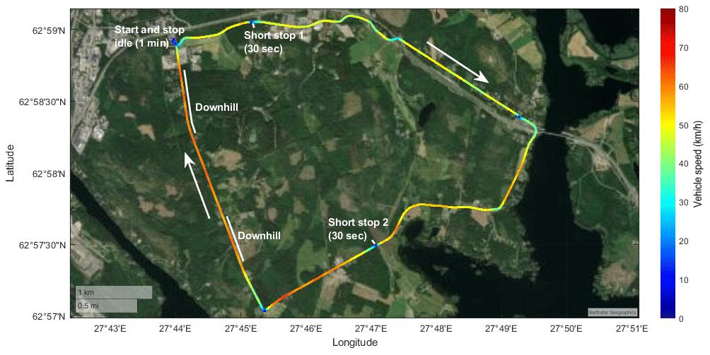
Figure 1 Driving route consisting of low-traffic small roads in Siilinjärvi, Finland. The coloured line indicates an example drive with the speed profile (colour). Start and stop locations were the same position at a parking lot of a local fuel station. Two artificial short stops were introduced along the test route to simulate traffic lights. Downhill sections that are used in “Results and discussion” are indicated by white lines on the side of the route marking. Source: Earthstar Geographics.

2 Methods

2.1 Experiments

Particle number concentrations and CO₂ concentrations in exhaust plumes of six passenger vehicles (three diesel and three petrol) were measured with the chase method during wintertime, in February in Siilinjärvi, Finland (Fig. 1). The time and the location were selected because the main purpose of the measurement campaign was to study wintertime real-world vehicle emissions, which is in the scope of future studies, applying methods introduced in this publication. The measurement instruments were installed inside the mobile laboratory of Tampere University (Aerosol and Trace Gas Mobile Laboratory, ATMo-Lab; Simonen et al., 2019; Rönkkö et al., 2017). Data from the OBD and GPS from the test vehicles were saved at a 1 s time resolution (Fig. 2). The chase route was 13.8 km long including uphill and downhill driving, stops, accelerations, and steady driving, as well as artificial short stops to simulate traffic lights. The route selection was chosen bearing two major principles in mind. On the one hand, the starting point was a fuel station with enough space for parking the test vehicles overnight and a connection to the electric grid to be used with electrical preheaters, and spaces were regularly cleared of snow. On the other hand, the station was located close to roads ideal for tests: they were in a good condition and were maintained well during winter, and the traffic rates were very low, implying that the background exhaust plumes are negligible. The route was also well suited for this study because it included steep and long downhill sections.

The test protocol included idling engine at the beginning for a short period, driving the route, stopping at two predetermined stops, and finishing the route at the start location. The time stamps of passing vehicles and other possible external emission sources were recorded during the drives.

Table 1 Information on the studied vehicles. DPF: diesel particulate filter, PPF: petrol particulate filter, MHEV: mild hybrid electric vehicle, SCR: selective catalytic reduction.

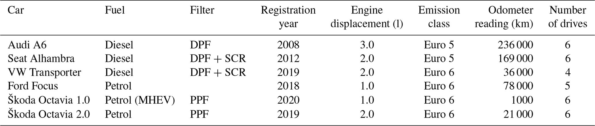
Information about the vehicles, individual drives, and outside temperatures are shown in Table 1. During the test period of 4 d, the outside temperature varied between −9 and −28 ^∘C. The fleet included three (Euro 5–6) diesel vehicles (two passenger cars and one van) and three (Euro 6) petrol vehicles (passenger cars). The number of measured drives totalled 33; in addition, there was a drive for every measurement day for measuring ambient background concentrations along the route. Of these, 11 drives were dedicated to subfreezing cold-start measurements (cold start in subfreezing temperatures), 12 were dedicated to preheated cold-start measurements (using electric preheaters or fuel-combusting auxiliary heaters), and 10 were dedicated to hot-start measurements (the engine had been heated to its normal operating temperature by driving).

2.2 Measurement setup

The measurement setup, including only the devices of which data are involved in this study, is presented in Fig. 2. The number concentration of particles larger than 23 nm in diameter (N) was measured with an Airmodus model A23 condensation particle counter (CPC), and the CO₂ concentration was measured with a LI-COR LI-840A analyser. The exhaust sample was drawn to the instruments through a sampling inlet installed on the front bumper of the vehicle. Before the CPC, the sample was diluted with a set of bifurcated flow diluters ($\text{DR}=\mathrm{158}\pm \mathrm{14}$). The drives were also recorded with a video camera installed on the windshield, and the ATMo-Lab location was recorded using GPS. OBD data from the chased vehicle were collected using OBDLink LX Bluetooth device (OBDLink^® LX, 2023). All the devices were recording data with a 1 s time resolution, which were averaged to a time resolution of 5 s. Averaging makes the data more robust to small (1–2 s) time differences between measurements from the vehicle (OBD) and variables measured with ATMo-Lab.

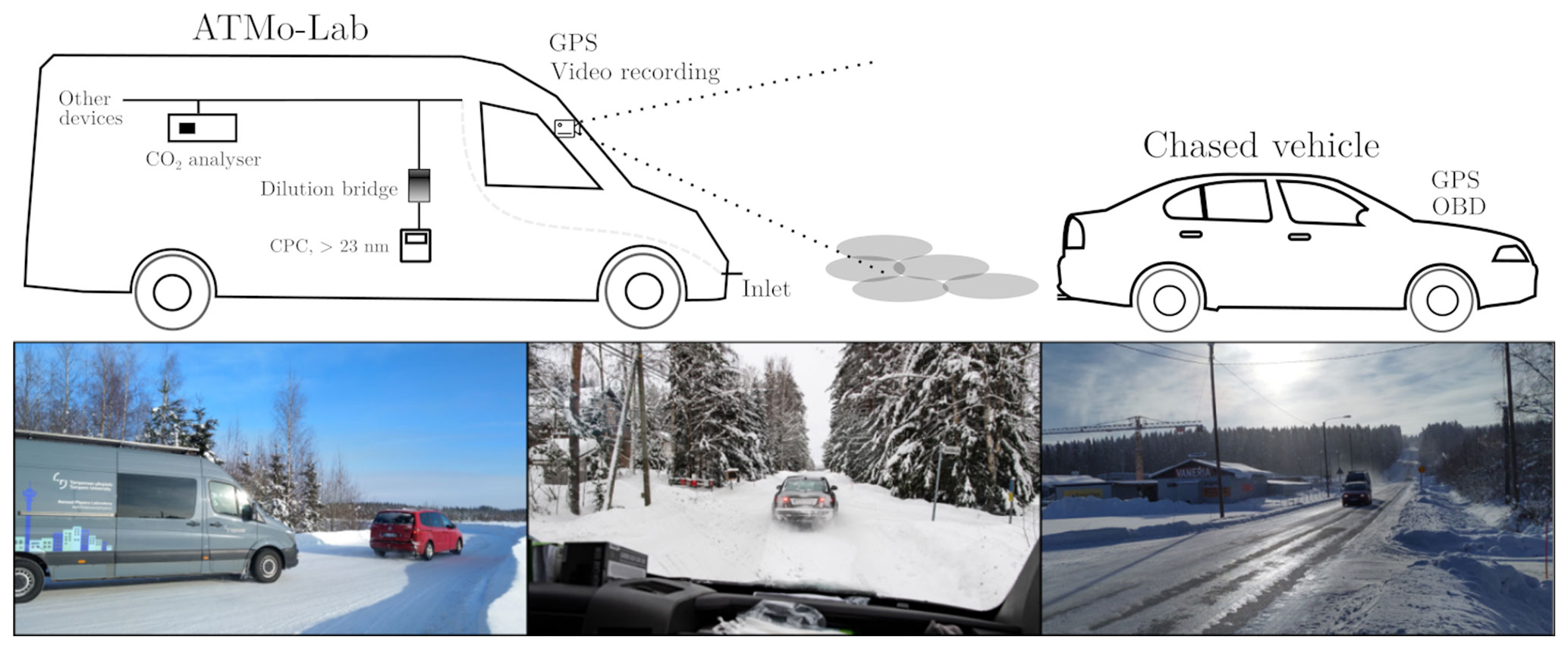
Figure 2 Schematic view of the measurement setup used in this study and example photos from the chase route for illustration of the chase measurements. In addition, other devices were installed, but their data were not used in this study.

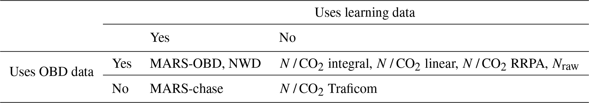
Table 2 Division of the methods for calculating the EF of a vehicle. OBD data are the mean of the data collected from the chased vehicle (see also Fig. 2), and learning data are the mean of the data collected from other drives of the same vehicle and from other vehicles (including data from ATMo-Lab, as well as from OBD if its data are used). Methods are introduced in more detail in Sects. 2.3.1–2.3.7. RRPA: robust regression plume analysis.

2.3 Methods for calculating EF

The methods we use are mostly modelling DR and observed differences between measured and background concentrations and based on those calculating the EF of a vehicle. Used methods (introduced more in detail in the following sections) for calculating EF can be divided into four categories based on whether the OBD data are used in the method and whether the method needs some additional (hereafter learning) data from other vehicles to evaluate the effect of some variables (e.g. speed change) to the emissions. Table 2 shows all the methods used in this study. All methods are introduced in Sect. 2.3.1–2.3.7. Table 3 summarizes the main differences of the methods described in Sect. 2.3.1–2.3.7 and shows the formulas used to calculate the EF in each of the methods.

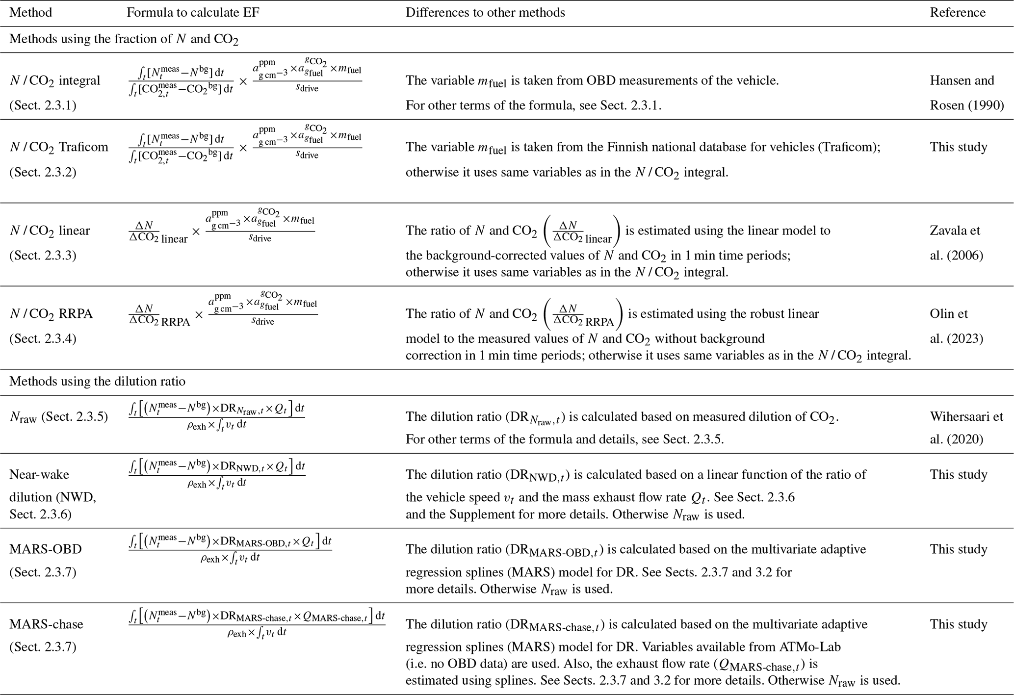
Table 3 Summary of the methods used in this study. Formulas to calculate EF, main differences to other methods, and references to the literature describing the method. Methods are introduced in more detail in Sect. 2.3.1–2.3.7.

The dataset used in this study was limited to considering only times when the chased vehicle was moving; i.e. its speed was positive. Also, the effect of the chase distance, i.e. the distance between the chased vehicle and ATMo-Lab, was assumed to be constant, not affecting the dilution ratio of emissions. Based on our estimation, the chase distance was between 5 and 10 m when the chased vehicle was moving. Unfortunately, the GPS data from the chased vehicle and ATMo-Lab were not accurate enough, so the changes in the chase distance could have been estimated from the GPS data.

Methods that require data to be fitted before application into the DR estimation or EF calculation were fitted using DR calculated from the N_raw method as a response variable. Only the data from the times with exhaust mass flow rates (Q) exceeding 0.3 g s⁻¹ and fuel flow rates exceeding 0.02 g s⁻¹ were used in forming models, which were then used for all data, also including the times with the flow rates below those limits.

Other methods of modelling DR (the NWD and MARS methods, described below) are based on the observed linear or non-linear dependencies between DR and an explanatory variable(s). These methods assume that the factors affecting DR measured in the situations where the measured vehicle is not in the engine-motoring mode can also be extrapolated to situations with the motoring mode. Hence, for the downhill sections, the following methods do not calculate the DR based on the measured CO₂; instead, they use other parameters not based on CO₂ (some examples include vehicle speed v_t, exhaust flow rate Q, and the vehicle rear shape) to estimate the DR.

For calculating EF and its uncertainty, bootstrap sampling (Efron, 1979) has been used to estimate the uncertainty in EF calculations. A bootstrap sample is a random sample of observations (an observation is a time point) with replacement; i.e. one observation can occur multiple times in a bootstrap sample. The analysis, e.g. fitting the model and calculating the EF, is performed for this bootstrap sample. Multiple bootstrap samples are usually taken; here 100 is the number of samples.

Bootstrapping helps to estimate the whole uncertainty, in this case the uncertainty related to e.g. differences in the vehicle-driving profile, possible uncertainties in time allocation, and uncertainty in model fitting. Bootstrapping is useful when estimating complex estimators or their uncertainty, without (here) explicitly estimating uncertainties of single sources of uncertainty and the covariance structure of uncertainties.

2.3.1 N / CO₂ integral

The simplest method to calculate EF is based on N / CO₂ measured from the diluted exhaust. The method was introduced by Hansen and Rosen (1990) and has been widely used since. It is based on the relation of the excess CO₂ ($\mathrm{\Delta }{\mathrm{CO}}_{\mathrm{2}}={\mathrm{CO}}_{\mathrm{2},t}^{\text{meas}}-{{\mathrm{CO}}_{\mathrm{2}}}^{\text{bg}}$) and particle concentration ($\mathrm{\Delta }N=N_t^{\text{meas}}-N^{\text{bg}}$). Here the superscripts “meas” and “bg” denote measured and background concentrations, respectively. Here t denotes that the measured concentrations have been measured specifically at time t, whereas the background concentrations have been defined as a median of the background measurement measured at the same route on the same day. However, the method by Hansen and Rosen (1990) uses the following integral form (over a longer measurement period than e.g. 1 s) to diminish possible uncertainties caused by imperfect time synchronization of the devices measuring CO₂ and the studied pollutant:

$$\begin{array}{}\text{(1)}& \begin{array}{rl}{\text{EF}}_{\mathrm{\Delta }\mathrm{N}/\mathrm{\Delta }{\mathrm{CO}}_{\mathrm{2}}}=& {\displaystyle \frac{{\int }_t[N_t^{\text{meas}}-N^{\text{bg}}]\mathrm{d}t}{{\int }_t[{\mathrm{CO}}_{\mathrm{2},t}^{\text{meas}}-{{\mathrm{CO}}_{\mathrm{2}}}^{\text{bg}}]\mathrm{d}t}}\\ & \times {\displaystyle \frac{a_{\mathrm{g}{\mathrm{cm}}^{-\mathrm{3}}}^{\text{ppm}}\times a_{g_{\text{fuel}}}^{g_{{\mathrm{CO}}_{\mathrm{2}}}}\times m_{\text{fuel}}}{s_{\text{drive}}}},\end{array}\end{array}$$

where CO₂ concentrations are in parts per million (ppm) and particle concentrations (N) are 1 cm⁻³. $a_{\mathrm{g}{\mathrm{cm}}^{-\mathrm{3}}}^{\text{ppm}}$ is the conversion factor for CO₂ from parts per million (ppm) to grams per cubic centimetre (g cm⁻³; ${\mathrm{10}}^{\mathrm{6}}/\mathrm{0.0018}=\mathrm{5.55}\times {\mathrm{10}}^{\mathrm{8}}$, where 10⁶ is a number of molecules and 0.0018 is the approximate density of CO₂ in g cm⁻³ at 20 ^∘C), $a_{g_{\text{fuel}}}^{g_{{\mathrm{CO}}_{\mathrm{2}}}}$ is the conversion factor for $g_{{\mathrm{CO}}_{\mathrm{2}}}$ to g_fuel ($\mathrm{2392}/\mathrm{750}=\mathrm{3.189}$ for petrol and $\mathrm{2640}/\mathrm{835}=\mathrm{3.162}$ for diesel, where 2392 and 2640 are the approximate masses of CO₂ produced in grams per litre of fuel for petrol and diesel, respectively; Innovation Norway, 2023), and 750 and 835 are the approximate densities in grams of fuel (g l⁻¹) for petrol and diesel, respectively. Those densities are within the ranges of densities provided by one major fuel supplier in Finland (Neste, 2023a, b). m_fuel is the mass of the used fuel (in g, from OBD data), and s_drive is the length of the drive (in km). In this study, EF is calculated over the whole measurement period, and EF is expressed as 1 km⁻¹. This method (and all other N / CO₂ method versions) is based on the assumption that CO₂ and the pollutant dilute equally in an exhaust plume and that the amount of emitted CO₂ is directly related to the fuel consumption. Whereas the N / CO₂ integral method is robust to imperfect time synchronization and to the engine-motoring events (because the integral in the denominator never becomes very small, unlike in cases with e.g. 1 s resolution), the method, however, assumes also that EF is constant during the integration time period in chase measurements (Olin et al., 2023).

2.3.2 N / CO₂ Traficom

The N / CO₂ Traficom method is calculated similarly to the N / CO₂ integral method, over the whole measurement period, but the fuel consumption m_fuel is estimated from the national vehicle database (Traficom) instead of using actual consumption from OBD. Traficom consumption values are based on the values provided by the manufacturer of the vehicles. The values in the database are the average consumptions (in units of per 100 km), and hence the actual consumption at certain times might be over or under the consumption value in the database. Using the fuel consumption estimation from the register makes the method independent of OBD data; i.e. the method can be calculated directly based on the measurement data from ATMo-Lab. This kind of a method, which does not OBD data, is suitable e.g. for real-world emission-monitoring approaches for private vehicles driving on public roads. We have used constant fuel consumptions reported for combined driving (combining urban and extra-urban driving) that are between 4.6 (Ford) and 7.6 L (VW) of fuel per 100 km.

2.3.3 N / CO₂ linear

The N / CO₂ linear method used e.g. by Zavala et al. (2006) was also tested in this study. The method estimates N / CO₂ by fitting a line for ΔN and ΔCO₂. The slope of that line is used to replace the first fraction term in Eq. (1) when calculating EF. The used linear model has an assumption that the line passes the origin; i.e. with no emitted CO₂, no particles are emitted. Therefore, non-exhaust particles are not counted. This method also assumes that EF is constant during the time period used for fitting. However, as the drives cannot be assumed to have a constant EF due to multiple different sections of driving, the linear model is fitted separately to 1 min time periods, in which the vehicle can be assumed to have a more constant EF throughout the period. For the periods when the slope is estimated to be negative, the EF is set to 0.

2.3.4 N / CO₂ RRPA

The RRPA (robust regression plume analysis) method presented in Olin et al. (2023) is based on the N / CO₂ linear method but without a need to determine the background concentrations of N and CO₂. Similarly to the N / CO₂ linear method, the slope is used to replace the first fraction term in Eq. (1) when calculating EF.

Contrary to the N / CO₂ linear method, this method uses a robust linear model (in this study using the rlm function in the R environment; R Core Team, 2022) for fitting the line. We used robust linear regression instead of an ordinary least-squares approach because the data contain a varying number of data points which can be considered outliers, from a statistical point of view, and those could bias the fit for the slope in an ordinary least-squares estimation (Mikkonen et al., 2019). The robust regression automatically weighs down the possible outliers by giving less weight to the data points that are not close to the estimated line. Hence, momentary disturbances (such as those from other pollutant sources near the measurement location) should not disturb the estimation of the slope. As for the N / CO₂ linear method, the N / CO₂ RRPA method assumes a constant EF for the fitted period and is also fitted to 1 min time periods. For the periods when the slope is estimated to be negative, the EF is set to 0.

2.3.5  N_raw

A bit more advanced method (based on the method by Wihersaari et al., 2020) to calculate DR and EF uses the measured and raw concentrations of CO₂ and the exhaust mass flow rate (Q):

$$\begin{array}{}\text{(2)}& {\displaystyle }{\text{DR}}_{N_{\text{raw}},t}={\displaystyle \frac{{\mathrm{CO}}_{\mathrm{2},t}^{\text{raw}}-{{\mathrm{CO}}_{\mathrm{2}}}^{\text{bg}}}{{\mathrm{CO}}_{\mathrm{2},t}^{\text{meas}}-{{\mathrm{CO}}_{\mathrm{2}}}^{\text{bg}}}},\text{(3)}& {\displaystyle }{\text{EF}}_{N_{\text{raw}}}={\displaystyle \frac{{\int }_t[\left(N_t^{\text{meas}}-N^{\text{bg}}\right)\times {\text{DR}}_{N_{\mathrm{raw}},t}\times Q_t]\mathrm{d}t}{{\mathit{\rho }}_{\text{exh}}\times {\int }_t{v}_t\mathrm{d}t}},\end{array}$$

where $N_t^{\text{meas}}$ is the measured particle number concentration, N^bg is the estimated background particle number concentration, ${\mathrm{CO}}_{\mathrm{2},t}^{\text{raw}}$ is the concentration of CO₂ in the raw exhaust (calculated from the OBD data), ${{\mathrm{CO}}_{\mathrm{2}}}^{\text{bg}}$ is the estimated CO₂ background concentration, ρ_exh is the exhaust density (air density at the standard temperature of 20 ^∘C used here), and v_t is the vehicle speed. We denote the method as the N_raw method from here onwards. This method can be thought of as the best-performing model in a real-world chasing situation with a varying EF and DR. However, this method requires well-synchronized data; 5 s time resolution was used, as it is not so prone to errors caused e.g. by engine-motoring events.

2.3.6 Near-wake dilution (NWD)

In the NWD method, we build a robust linear model for DR as a linear function of the ratio of the vehicle speed v_t and the mass exhaust flow rate Q, taking also into account the shape of the vehicle's rear and the fuel used. The method is based on the assumption that the outdoor air passing by the vehicle's rear while driving dilutes the exhaust plume and that the dilution is proportional to the ratio of the mass flows passing the rear and exhausted from the tailpipe (Chang et al., 2012). The method minimizes the weighted linear model (iterated reweighted least-squares robust regression):

$$\begin{array}{}\text{(4)}& {\text{DR}}_{\text{NWD},t}=\mathit{\gamma }+\mathit{\kappa }{\displaystyle \frac{v_t}{Q_t}},\end{array}$$

where the dilution ratio at time t (DR_t) used to fit the model is calculated from the OBD chase measurement data as in the N_raw method (Eq. 2). Parameters γ and κ are coefficients fitted for every vehicle measured in this study. A more detailed derivation of the formula and detailed discussion about the possible variables that are related to parameters γ and κ are presented in the Supplement. The NWD model is fitted separately for each vehicle, except when the data from the studied vehicle are not used to fit a model (Fig. 6). In that case, the rear shape has been used as a categorical variable for the five-vehicle data to fit the NWD model. Categorical variables b₁ and b₂ estimate the effect of different rear types on DR: ${\text{DR}}_{\text{NWD},t}=\mathit{\gamma }+b_{\mathrm{1}}+(\mathit{\kappa }+b_{\mathrm{2}})\frac{v_t}{Q_t}$.

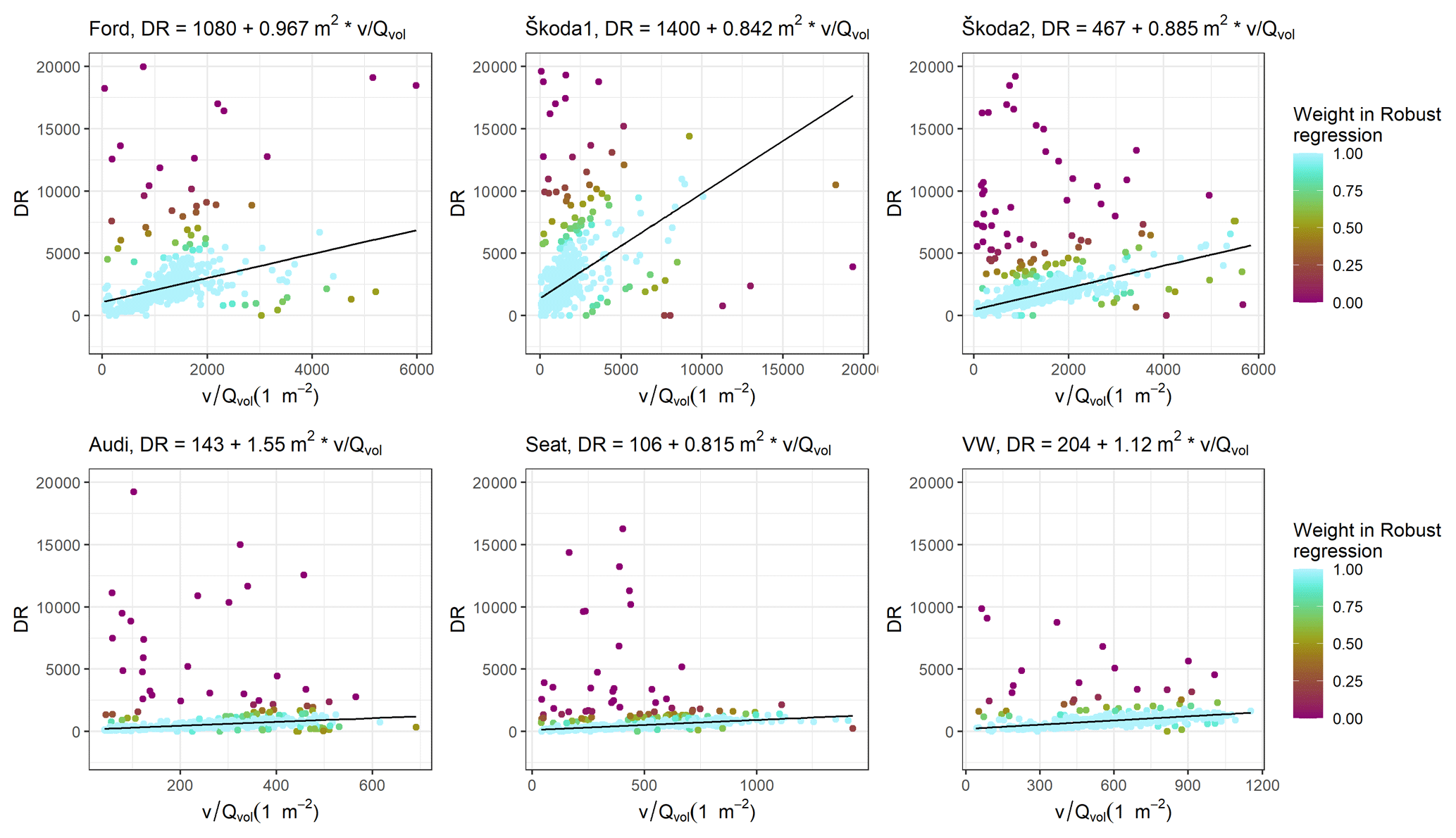
Figure 3 Robust linear regression fits for DR for each vehicle used in the NWD method. The colour represents the weight of the observation in the final robust linear fit. The equations of the linear fits are shown in the titles of each subplot. The volumetric exhaust flow rate of $Q_{\text{vol}}=\frac{Q}{\mathrm{3.6}\cdot {\mathit{\rho }}_{\text{fuel}}}$ has been used in this figure instead of the mass flow rate used elsewhere because the NWD model is based on the volumetric flows.

As the model is only dependent on the speed and exhaust flow, the model assumes that the distance from the vehicle remains constant and is independent of the speed (the effect of the distance is incorporated into the κ and γ parameters). Constant driving distances were attempted to be maintained during these chase measurements. DR is calculated for all data points using the modelled dependency (presented later in Fig. 3).

EFs with the NWD method were then calculated similarly to the N_raw method in Eq. (1), with a different method to calculate the dilution ratio being the only difference between the methods. The NWD method is robust to engine-motoring events because the CO₂ concentration is not involved in the equation used to calculate EF (after fitting the κ and γ parameters). In addition, the method can possibly be used to determine non-exhaust emissions as well.

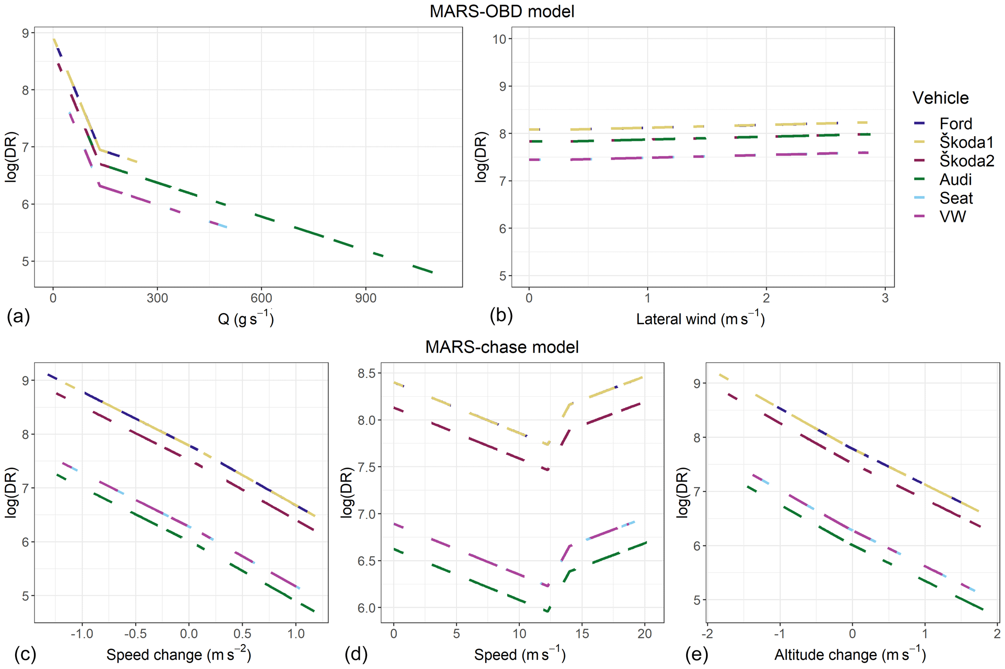
Figure 4 Multiple adaptive regression spline fits for the logarithm (natural) of DR shown for each variable used in MARS-OBD (a, b) and in MARS-chase (c, d, e). Different coloured lines show the regression splines for each vehicle (see also the categorical variables in the method description in Sect. 2.3.7), with some splines (Ford and Škoda1, Škoda2 and Audi) overlapping with each other.

2.3.7 Multivariate adaptive regression splines (MARS)

We used multivariate adaptive regression splines (MARS; Friedman, 1991; Hastie et al., 2009) to model the dependency of DR on certain variables that could affect the dilution of exhaust, i.e. vehicle exhaust flow rate, speed, speed change (acceleration), altitude change, and direction of wind. Besides variables that are fitted with splines, two categorial variables describing the rear shape and fuel type used in the vehicle were used. Those categorical variables affect only the level, not the shape, of the spline (see Fig. 4).

To avoid overfitting, i.e. that the model fits well to the learning data but is not generalizable to any new dataset, we used 5-fold cross-validation (Hastie et al., 2009). In 5-fold cross-validation, the dataset is divided into five distinct subsets of the same size. Then four of those subsets are used to train the model (training dataset), and one is used to test the fit of the model to new dataset (testing dataset). This is repeated five times so that each subset is used once as a testing dataset.

We built two methods based on MARS: one is based on all variables (OBD data and the data from chase measurement; a method called MARS-OBD), and the other one is based on the measured data consisting of only variables that are available with remote sensing methods (a method called MARS-chase).

EFs from the MARS methods were calculated similarly to the N_raw method (Eq. 1), with the only difference to N_raw in how the DR is calculated. As for NWD, DR is calculated for all data points using the modelled dependency (presented later in Fig. 4). MARS models are also robust for engine-motoring events or even for non-exhaust emissions, like the NWD model, because the CO₂ concentration is not used (after the model construction). In addition, the MARS-chase model can be used in real-world emission-monitoring approaches.

3 Results and discussion

3.1 Fitting the NWD model parameters

Our results indicate that DR can be approximated with a linear function of the ratio of v_t and Q; hence, it was used as one method to estimate DR. Figure 3 shows the robust linear regression fits between DR and $\frac{v_t}{Q}$.

According to the results, in addition to $\frac{v_t}{Q}$, we suppose that modelled DR is mostly affected by the rear shape of the vehicle (included in the parameter κ). Generally, the values of $\frac{v_t}{Q}$ are higher for the petrol vehicles compared to the diesel vehicles, due to lean-burn combustion used in diesel engines. This also results in higher values of DR (determined with Eq. 2) for the petrol vehicles.

3.2 Constructing the MARS models

Figure 4 shows the behaviour of the splines in the measured data between DR and the predictor variables used in the MARS models. The shape of the splines is the same for all vehicles, as it is defined from the full dataset, but the level varies due to different properties of the vehicles, such as fuel and presumably the rear shapes.

The variables used in the models shown in Fig. 4 are organized so that the variables in the upper row are for the method also using the OBD data from the chased vehicle (MARS-OBD) and the variables in the lower row are for the method using only variables from ATMo-Lab (MARS-chase). With the MARS-OBD method, changes in Q explain most of the changes observed in DR, and the dependency of Q on DR is as expected from the concept behind the NWD model. In addition to Q, the wind component calculated abeam of the vehicle was seen to affect the DR, but the effect is very minor. Unlike in the MARS-chase method, variables such as speed change and altitude change were not needed (based on their effect on the model fit, measured with R² values) in the MARS-OBD method, which indicates that the changes in Q (and slightly in the lateral wind speed) sufficiently explain most of the changes in DR.

For the MARS-chase method, the effect of Q was replaced by using several variables that could explain the power generated by an engine – and thus Q. The result seems to be in line with theory, with the most evident changes to DR being caused by changes in driving speed (e.g. when accelerating) and altitude (e.g. when driving uphill) and the absolute speed of a vehicle (due to air drag). Observed dependencies of those variables with DR were described with piecewise linear splines with one or two threshold values (knots). The effect of changes in speed and altitude were close to linear. The effect of v_t was not linear, as the DR had its minimum after a threshold speed slightly higher than 10 m s⁻¹.

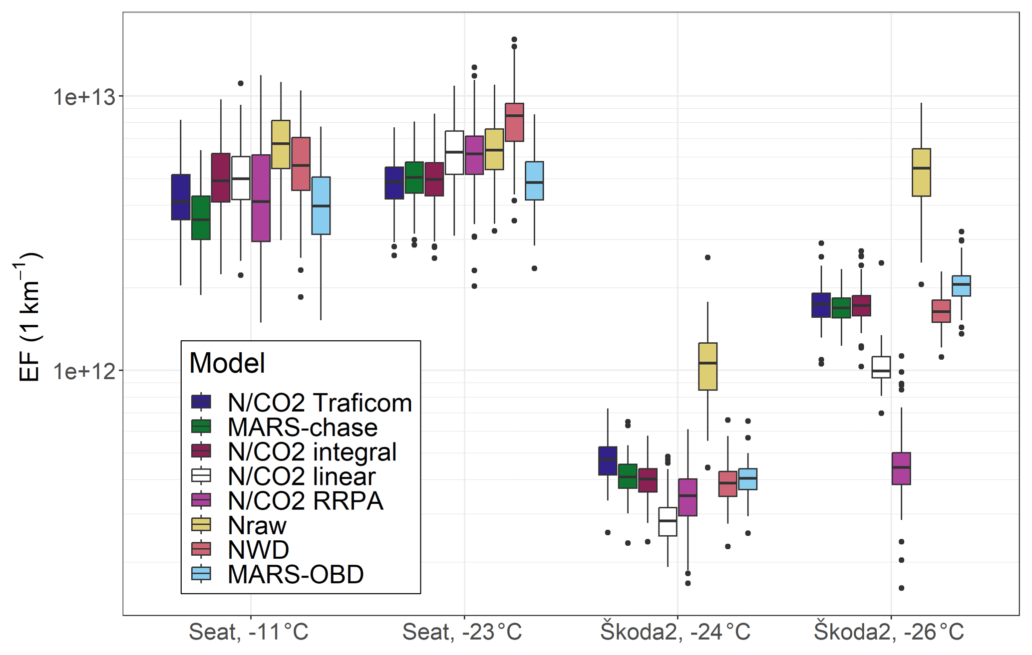
Figure 5 Emission factor examples of > 23 nm particles for Seat and Škoda2 with hot starts, except for Seat at −11 ^∘C, which has a subfreezing cold start, and Škoda2 at −26 ^∘C, which has a preheated cold start. Results are calculated from 100 bootstrap samples (see Sect. 2.3 for the description of bootstrap sampling). Whiskers represent the distribution of EFs in different bootstrap samples.

3.3 Comparison of the EF calculation methods for the whole drive

When the calculated DR estimates were applied on the EF calculation for the whole drive, it was seen that the results are mostly similar with all methods. Figure 5 illustrates how the calculated EF varies with different methods when applied on two different vehicles, one with a petrol and one with a diesel engine, on two different drives with varying outside temperature.

The results in Fig. 5 give confidence to the EF calculation with varying information in use, as the methods with different background information end up mostly being within an order of magnitude. This is specifically good news for monitoring-type measurements being performed on road with limited information on the monitored vehicle. However, there can still be some notable differences between the methods, for example the difference of a factor of 2–3 between the N_raw and other methods for Škoda2 at −24 ^∘C. The clearest anomalies from the consensus of EF are N / CO₂ RRPA for the drive of Škoda2 at −26 ^∘C being 25 % to 45 % of the EFs given by methods other than N_raw and N / CO₂ linear, with the N_raw method for both Škoda2 drives showing EFs 2 to 4.2 times higher than most of the methods (other than N / CO₂ linear and N / CO₂ RRPA). For RRPA some of the 1 min interval EFs were estimated to be 0, which probably explains the lower EFs calculated for that method. For the N_raw method, the difference comes from the time points where the dilution ratio is estimated to be larger, e.g. in the NWD and MARS models, i.e. points clearly above modelled lines in Figs. 3 and 4. If the measured concentration of particles above the background ($N_t^{\text{meas}}-N^{\text{bg}}$) is high enough for those points, it also results in a high EF for that point.

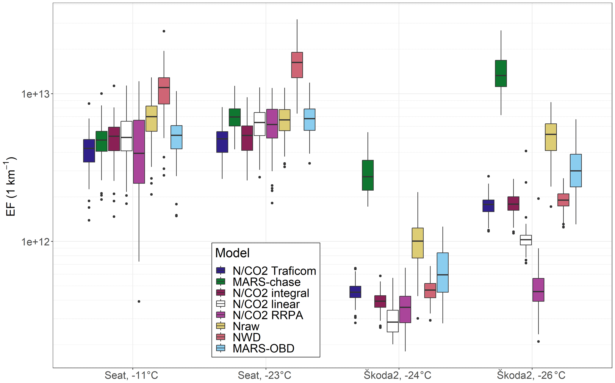
Figure 6 Emission factors for the drives of which data are omitted (details in Sect. 3.3) from the model construction (MARS-chase, NWD, MARS-OBD) for Seat and Škoda2 with hot starts, except for Seat at −11 ^∘C, which has a subfreezing cold start, and Škoda2 at −26 ^∘C, which has a preheated cold start. Results are calculated from 100 bootstrap samples (see Sect. 2.3 for the description of bootstrap sampling). Whiskers represent the distribution of EFs in different bootstrap samples.

The methods that use learning data (the MARS methods and the NWD method; see Table 2) were validated with leave-one-out-type cross-validation by omitting one of the vehicles from the model fitting and then by applying the fitted coefficients to predict the EFs for the omitted vehicle. The results in Fig. 6, confirming the findings in Fig. 5, show that the constructed methods can also calculate the EFs for the vehicle omitted from the model construction. For the methods that do not use learning data (all N / CO₂ methods and the N_raw method), i.e. data from the other drives to form a model, the results are almost the same (bootstrap sampling can change the calculated EFs slightly) as in Fig. 5. For Škoda2, the MARS-chase method shows EF values higher than the other methods in Fig. 6. This is probably because the data measured with Audi (being the only vehicle having a similar rear shape to Škoda2) were used in the MARS-chase model to estimate the effect of the rear shape on the DR (see Sect. 2.3.7 for categorical variables and Fig. 3 for the fits). However, using the data from a diesel vehicle in modelling DR for a petrol vehicle may not work properly due to different dilution mechanics (as is also observed from the different fitting parameters obtained with using the NWD model), even though the fuel-type parameter for Škoda2 is different than for Audi. In addition, Audi is the only vehicle in this study with two exhaust pipes on both sides of the vehicle rear; therefore, the dilution mechanics may differ notably from the other vehicles. Thus, the rear shape parameter (constant categorial variable used to estimate the effect of the rear shape on DR) might have increased the estimated DR for Škoda2 and hence also the estimated EF. One solution for this issue would be to increase the sample size of the vehicles, probably leading to a better estimate for the rear shape of Škoda2 in the MARS-chase method. For Seat, the MARS-chase method gives similar results to the other methods; however, the NWD method gives slightly higher EFs than the other methods. This is due to imperfect modelling of the dilution ratio of Seat based on the model from five other vehicles. This indicates that EFs could be calculated in situ based on the measurements from ATMo-Lab and OBD if the OBD data are required in the method. The increase in the number of vehicles in the learning data would probably increase the accuracy of the methods that require learning data, including the MARS-chase method as well.

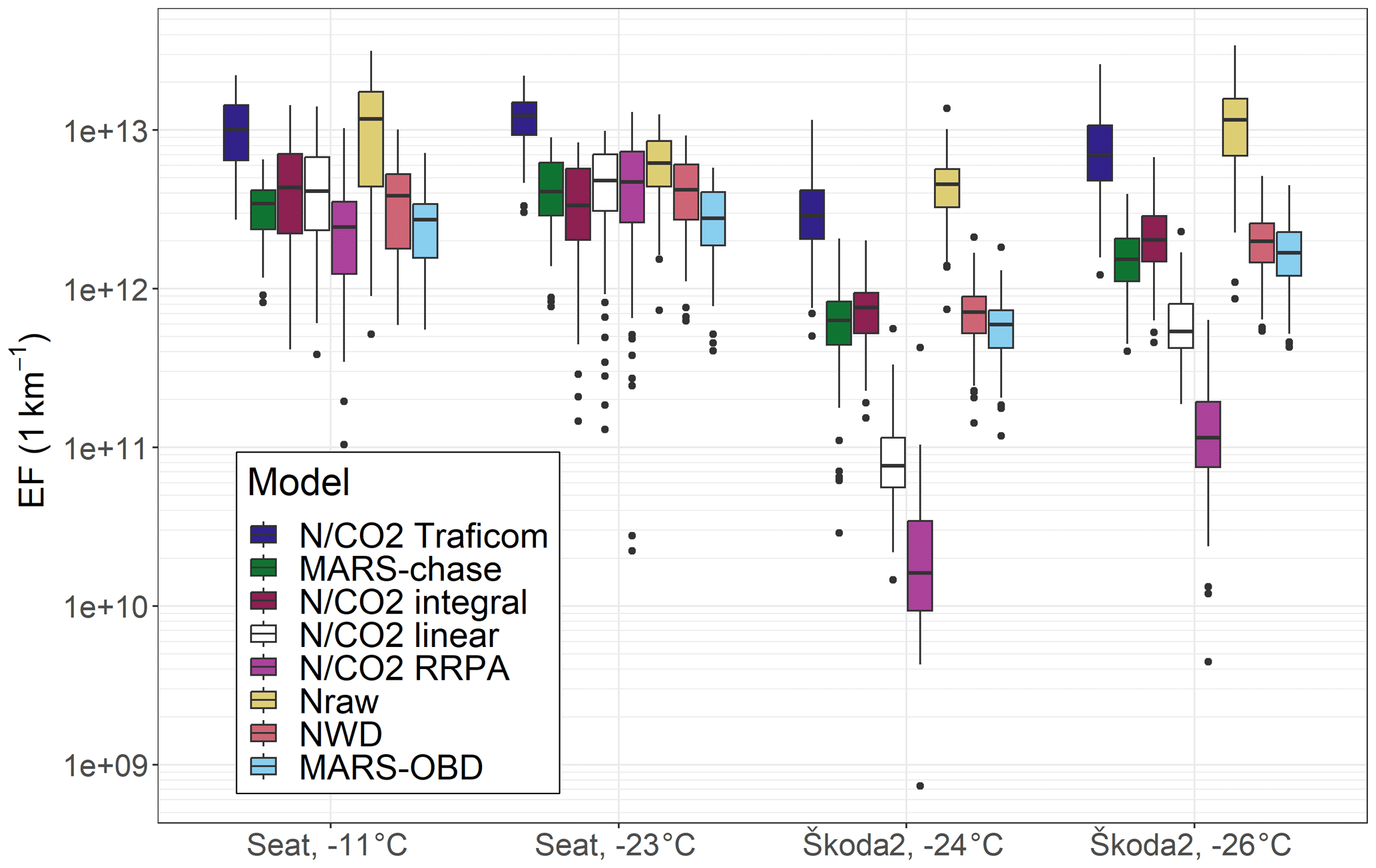
Figure 7 Emission factors of > 23 nm particles for downhill sections and for Seat and Škoda2 with hot starts, except for Seat at −11 ^∘C, which has a subfreezing cold start, and Škoda at −26 ^∘C, which has a preheated cold start. Results are calculated from 100 bootstrap samples (see Sect. 2.3 for the description of bootstrap sampling). For Škoda2 N / CO₂ RRPA, some EFs (89 for Škoda2 at −24 ^∘C and 39 for Škoda2 at −26 ^∘C) are 0. Only EFs above 0 are shown in this figure.

3.4 Comparison of the EF calculation methods for the downhill section

When examining how the different methods perform in different driving conditions, such as the change in the altitude, Fig. 7 shows that, overall, the methods agree quite well for Seat, but there are a lot of discrepancies for Škoda2. It is obvious why the N / CO₂ Traficom method overestimates the EFs during the downhill section: the used-fuel consumption refers to the combined-driving fuel consumption data, i.e. to a much higher consumption than really occurs in downhill sections. In addition, the N_raw method gives relatively high estimates for EFs, especially for Škoda2. This is due to relatively low CO₂ values observed at the times with high particle emissions, resulting in higher DRs with the N_raw method compared to the other methods. N / CO₂ linear clearly shows lower EF values for Škoda2, which is similar but less pronounced, in Figs. 5 and 6. For the RRPA method, many of the EF estimates for the bootstrap samples (89 out of 100 for Škoda2 at −24 ^∘C and 39 for Škoda2 at −26 ^∘C) are 0; i.e. for every minute interval (2 or 3 intervals in each bootstrap sample), the estimated linear dependency between N and CO₂ concentrations is negative, and hence the EF is estimated to be 0. The assumption of a constant EF is not valid in downhill sections, and the concentrations of N and CO₂, as well as exhaust flow rate, are mostly lower than the average of the whole round, whereas the DR, which is used in many other methods, is mostly higher than the average of the whole round. We believe that those are the reasons why RRPA is giving EFs that are so different compared to other methods for downhill sections.

Other methods (MARS-chase, N / CO₂ integral, NWD, and MARS-OBD) give similar values for EF. This is kind of expected as the methods are fitted using data from the full drives (as in the case in Figs. 5 and 7). Therefore, N / CO₂ is estimated mostly from the data with above-zero fuel consumption; hence, the number of particles emitted per additional CO₂ emitted should be estimated well. The other methods are also based on data with above-zero fuel consumption; thus, the dilution ratio for the downhill sections can also be estimated.

4 Conclusions

There are methods to define DRs and EFs that require OBD data from the vehicle under tests and methods that do not require these data. We conclude that most of the N / CO₂ methods are not suitable for transient driving, where EF is constantly changing during the drive, which is indicated by results that differ from the ones obtained with the other methods.

For those time points where the measured CO₂ is close to its background value, the new methods (the NWD and the MARS methods) work better than the old ones. Among these, the NWD method is physically more realistic and hence easier to interpret. We believe both the NWD and the MARS method introduced are extendable also to non-exhaust emissions. For NWD, the method is based on the estimated slope κ of the vehicle. For example, for tire emissions, if the emissions from the tires are C_raw and the mass exhaust flow rate of the emissions is Q, then $\text{EF}={\mathrm{C}}_{\mathrm{raw}}\times Q$. On the other hand, it was assumed that $\text{DR}=\mathit{\kappa }\times v/Q$. Then ${\mathrm{C}}_{\mathrm{raw}}={\mathrm{C}}_{\mathrm{meas}}\times \text{DR}={\mathrm{C}}_{\mathrm{meas}}\times \mathit{\kappa }\times v/Q$. For EF, we get $\text{EF}={\mathrm{C}}_{\mathrm{raw}}\times Q={\mathrm{C}}_{\mathrm{meas}}\times \mathit{\kappa }\times v$. Hence, an explicit value of mass exhaust flow rate Q is not needed to calculate the EF of non-exhaust emissions. The κ value can be estimated from the other vehicle with a similarly estimated dilution of emissions, or, in the case of a hybrid vehicle, κ can be determined during the time when the combustion engine is running. For MARS the basic idea is that from the test dataset of measurements, the dilution ratio of emissions could be estimated in different driving situations. Then in the new dataset, DR is estimated based on splines estimated from the test dataset.

In both methods, the emission factor of the non-exhaust emissions can be determined during the times when the vehicle is running with an electric engine only. For the non-exhaust emissions, some correcting coefficient for the dilution ratio might be needed. Both methods would require some prescribed database to characterize the effect of the vehicle's shape on DR. The number of required vehicles for the database can be from one (if the interest is only emissions of a specific vehicle) to several hundred vehicles (monitoring of emissions from random vehicles from the fleet).

The MARS methods are based on the dependencies of the measured variables on DR from the N_raw method. It fixes the problems of the N_raw method at the time points where DR is estimated to be very high with the N_raw method. On the other hand, the MARS methods do not have as clear a physical interpretation as the NWD method. The MARS methods are, however, very adaptive methods, and DR could be modelled using variables other than the ones used in this paper, which might increase the physical interpretability of the methods.

If the MARS methods were used with other variables, for their generalizability, it would be beneficial to use variables that are generally measured in the chase measurements. Positive sides of the MARS methods also include that, in the MARS-chase method, no variables measured directly from the vehicle diagnostics are not needed. This enables the observation in the middle of traffic, as well as in driving situations where EF and DR cannot be assumed to be constant.

The weakness of these methods is that the time points with a vehicle speed of 0 have been omitted in this study. This limits the usability of the method in e.g. urban conditions where the vehicle is stationary a significant part of the time. In this study we wanted to focus especially on times when the vehicle is moving, including downhill sections, and the fuel flow rate is 0 or close to 0. The times when the vehicle is stationary could be added to the methods (MARS and NWD) by separately considering the speeds of 0. In the first place, it could be implemented by using e.g. the N_raw method for those times.

Vehicle chase studies in the future will not only be limited to the determination of the exhaust-originating species, since the NWD method could be used to define the non-exhaust particle emission originating e.g. from the brakes and tires of the vehicle under the test. In addition to being an important tool in emission research, especially in real-world emission factor determination including for semi-volatile particles, the chase method has potential to be a monitoring tool for vehicle fleets for official purposes: high-emitting vehicles could be identified while driving with simultaneous particle and CO₂ sensor signals and processed for further detailed measurements according to e.g. the new PTI protocol, where particle number concentrations are measured on low idle.