the Creative Commons Attribution 4.0 License.
the Creative Commons Attribution 4.0 License.
 | 03 Apr 2024
Effects of clouds and aerosols on downwelling surface solar irradiance nowcasting and short-term forecasting
Kyriakoula Papachristopoulou
Ilias Fountoulakis
Alkiviadis F. Bais
Basil E. Psiloglou
Nikolaos Papadimitriou
Ioannis-Panagiotis Raptis
Andreas Kazantzidis
Charalampos Kontoes
Maria Hatzaki
Stelios Kazadzis
Solar irradiance nowcasting and short-term forecasting are important tools for the integration of solar plants into the electricity grid. Understanding the role of clouds and aerosols in those techniques is essential for improving their accuracy. In this study, we introduce improvements in the existing nowcasting and short-term forecasting operational systems SENSE (Solar Energy Nowcasting System) and NextSENSE achieved by using a new configuration and by upgrading cloud and aerosol inputs, and we also investigate the limitations of evaluating such models using surface-based sensors due to cloud effects. We assess the real-time estimates of surface global horizontal irradiance (GHI) produced by the improved SENSE2 operational system at high spatial and temporal resolution (∼ 5 km, 15 min) for a domain including Europe and the Middle East–North Africa (MENA) region and the short-term forecasts of GHI (up to 3 h ahead) produced by the NextSENSE2 system against ground-based measurements from 10 stations across the models' domain for a whole year (2017).
Results for instantaneous (every 15 min) comparisons show that the GHI estimates are within ±50 W m−2 (or ±10 %) of the measured GHI for 61 % of the cases after the implementation of the new model configuration and a proposed bias correction. The bias ranges from −12 to 23 W m−2 (or from −2 % to 6.1 %) with a mean value of 11.3 W m−2 (2.3 %). The correlation coefficient is between 0.83 and 0.96 and has a mean value of 0.93. Statistics are significantly improved when integrating on daily and monthly scales (the mean bias is 3.3 and 2.7 W m−2, respectively). We demonstrate that the main overestimation of the SENSE2 GHI is linked with the uncertainties of the cloud-related information within the satellite pixel, while relatively low underestimation, linked with aerosol optical depth (AOD) forecasts (derived from the Copernicus Atmospheric Monitoring Service – CAMS), is reported for cloudless-sky GHI. The highest deviations for instantaneous comparisons are associated with cloudy atmospheric conditions, when clouds obscure the sun over the ground-based station. Thus, they are much more closely linked with satellite vs. ground-based comparison limitations than the actual model performance. The NextSENSE2 GHI forecasts based on the cloud motion vector (CMV) model outperform the persistence forecasting method, which assumes the same cloud conditions for future time steps. The forecasting skill (FS) of the CMV-based model compared to the persistence approach increases with cloudiness (FS is up to ∼ 20 %), which is linked mostly to periods with changes in cloudiness (which persistence, by definition, fails to predict). Our results could be useful for further studies on satellite-based solar model evaluations and, in general, for the operational implementation of solar energy nowcasting and short-term forecasting, supporting solar energy production and management.
- Article
(6592 KB) - Full-text XML
- BibTeX
- EndNote


Climate change mitigation along with energy production in a sustainable manner can be addressed through the deployment of renewable energy technologies (Edenhofer et al., 2011; IPCC, 2022). Diverse renewable-energy technologies are being investigated worldwide, and their deployment has been increasing, with solar energy markets growing rapidly, such that they could become the major source of energy supplies in the coming decades (Arvizu et al., 2011; IEA, 2022). Since solar energy resources are strongly affected by atmospheric conditions, they are highly variable spatially and temporally. Therefore, there is a need for operational nowcasting and short-term solar forecasting for real-time energy production to better integrate solar energy exploitation technologies with national and international power systems. Under all skies, the availability of solar resources is primarily affected by clouds (e.g., Fountoulakis et al., 2021); for clear-sky conditions, it depends on the atmospheric composition, with the most important variables being aerosols (e.g., Papachristopoulou et al., 2022) and water vapor (e.g., Yu et al., 2021). Among those variables, clouds and aerosols are characterized by large temporal and spatial variability, making them key variables for solar energy applications. Continuously improved earth observation (EO) data (satellite-based and atmospheric models) are exploited to produce accurate estimates of spectral surface solar radiation in real time (nowcasting), which has numerous applications in different fields aside from the solar energy sector (e.g., Qu et al., 2014; Thomas et al., 2016; Kosmopoulos et al., 2018), like human health (e.g., Kosmopoulos et al., 2021; Schenziger et al., 2023). To increase the accuracy of those nowcasting and forecasting tools, it is imperative to understand the spatiotemporal variability of cloud and aerosol properties when implementing the tools.
Solar resource assessment at a particular location is important for planning and managing solar energy technologies. Ground-based measurements of surface solar radiation are only available for a few locations, with possible gaps in time. Those spatial and temporal gaps are filled by modeled estimates of surface solar radiation. Of particular importance are gridded surface solar radiation estimates with high spatial and temporal resolution and a wide coverage (up to the global scale) provided by satellite-based models or atmospheric models (see, e.g., an overview of those techniques in Sengupta et al., 2021). Due to their large area coverage and high temporal resolution, geostationary satellite data are used to produce estimates of surface solar radiation both in real time as an operational service and to generate historical archives based on long-term satellite measurements. Several methods exist for obtaining satellite estimates of surface solar irradiance. A well-established method considers cloud extinction through the cloud coverage index (Cano et al., 1986) or cloud index, calculated from normalized satellite reflectances. Using the cloud index, the transmission factor or the clear-sky index (also called the cloud modification factor; “CMF” hereafter) is calculated, which is finally multiplied by the results of a clear-sky model to retrieve the solar irradiance at the earth's surface (Hammer et al., 2003). This is the general idea behind the HELIOSAT method (Cano et al., 1986; Hammer et al., 2003) widely used in various European research projects and applications. The derivative Heliosat-2 method (Rigollier et al., 2004) is launched in real time by the SoDa service and produces the HelioClim-3 database (Qu et al., 2014), a real-time solar radiation database dating from February 2004 onwards. A more recent version of the HelioClim-3 database (Thomas et al., 2016) – version 5 (HC3v5) – combines the McClear clear-sky model (Lefevre et al., 2013; Gschwind et al., 2019) with cloud index values extracted from Meteosat Second Generation (MSG) satellite images. The Satellite Application Facility on Climate Monitoring (CM SAF) provides satellite-based estimates of surface solar radiation using data from Meteosat geostationary satellites. Currently, the third edition of the Surface Solar Radiation Data Set – Heliosat (SARAH-3, Pfeifroth et al., 2023a) – covers the period 1983–2020 as a climate data record (CDR) and is operationally extended into the present with a delay of a few days (Interim Climate Data Record (ICDR)). The retrieval algorithm MAGICSOL (Pfeifroth and Trentmann, 2023; Müller et al., 2015) is a combination of a modified Heliosat method to derive the effective cloud albedo (CAL) and the SPECMAGIC clear-sky model (Mueller et al., 2012). More available open-access satellite-based surface solar radiation climatological datasets based on the cloud index method can be found in Müller and Pfeifroth (2022).
There are also fully physical models that directly estimate surface solar radiation using radiative transfer models (RTMs) and geophysical parameters – including clouds (cloud and aerosol optical properties and total column values for water vapor and ozone content) and surface conditions – as inputs for a given atmospheric state. The combination of multi-channel information from geostationary satellites with cloud retrieval schemes provides cloud optical properties that can be explicitly used in RTMs to account for cloud extinction and finally to calculate the surface solar radiation. Parameterizations or look-up tables based on RTM simulations are used instead of direct radiative transfer calculations to optimize the computational time for operational use of the models. This is the case for the Heliosat-4 method (Qu et al., 2017), which is used in Copernicus Radiation Service (CAMS Radiation Service) estimates of surface solar irradiance. Their Heliosat-4 method is composed of two models that independently consider clear-sky and cloudy conditions. Specifically, the McClear model (Lefèvre et al., 2013; Gschwind et al., 2019) is used for calculations of cloud-free irradiances and the McCloud model for calculating the extinction of irradiance by clouds (through the clear-sky index), both of which are based on look-up tables (LUTs) to speed up calculations. The input cloud properties of the current CAMS Radiation Service v4 are retrieved by the adapted APOLLO Next Generation scheme from the MSG/SEVIRI (Spinning Enhanced Visible and Infrared Imager) satellite images (Schroedter-Homscheidt et al., 2022). The most recent version of the US National Renewable Energy Laboratory's (NREL's) gridded National Solar Radiation Database (NSRDB; 1998–2016; Sengupta et al., 2018) is also based on a fully physical model. This is the Physical Solar Model (PSM), which was developed by NREL and produces gridded surface solar irradiance estimates using satellite retrievals for clouds and other atmospheric properties from GOES data as input to the radiative transfer model.
The continued developments and improvements in satellite estimates of surface solar radiation made since the 1980s resulted in accurate real-time as well as climatological datasets (Qu et al., 2014; Urraca et al., 2017; Pfeifroth et al., 2023b; Qu et al., 2017; Schroedter-Homscheidt et al., 2022; Sengupta et al., 2018; Habte et al., 2017), although certain sources of biases and common factors that increase the uncertainty have been reported: an increase in the distance from the subsatellite point and more frequent occurrences of clouds (especially fragmented cloud cover), complex terrain, and bright surfaces (snow, desert). In addition, it is a challenge per se and increases the evaluation uncertainties when any model is validated at an instantaneous timescale. Gridded satellite estimates with ground-based point measurements of surface solar radiation differ not only due to model uncertainties but also due to the different spatiotemporal scales involved (satellite pixels represent a large area and large time intervals of a few minutes; ground-based measurements represent the area exactly over the station for smaller time intervals).
Motivated by the recent advances in satellite-based retrievals of surface solar radiation and building upon the knowledge of already-existing and well-established methodologies, an upgrade has been performed to an existing service that provides satellite estimates of surface solar radiation in real time. The aim is for the improved nowcasting system to be the basis of the new forecasting system. The Solar Energy Nowcasting System (SENSE) was developed under the EU project Geo Cradle by the Beyond Centre of EO Research and Satellite Remote Sensing at the National Observatory of Athens, Greece, in collaboration with the Physical and Meteorological Observatory at Davos of the World Radiation Center, Switzerland (Kosmopoulos et al., 2018). It is a combination of geophysical input parameters from satellite-based and model data sources and a neural network (NN) technique trained on precalculated surface solar radiation simulations (look-up table – LUT) using RTM. It uses the cloud optical thickness (COT) retrievals produced by the Application Facilities Support to Nowcasting and Very Short Range Forecasting (NWC-SAF) algorithm based on MSG satellite data and aerosol optical depth (AOD) forecasts from the Copernicus Atmospheric Monitoring Service (CAMS) as inputs to the NN to derive the surface solar radiation in real time. More details about the previous version of the SENSE service can be found in Kosmopoulos et al. (2018). In the same publication, the validation of this method showed good agreement on daily and monthly levels; however, various sources of uncertainties have been identified, mainly concerning the use of the NN (especially under high irradiance values), the COT input, and the structure and density of atmospheric parameters in the LUTs. The reason for the development of the new version of the model, called SENSE2, used in the present study was to minimize those uncertainties before using this model for the new forecasting system. For the new version of the model, it was decided that the fully physical approach of the model, which benefits from cloud optical property monitoring by the MSG satellites and recent advances in EO, would be retained, while the scheme that replaces the direct radiative transfer calculations would be improved.
The solar energy forecasting methods are categorized into three base methods (Sengupta et al., 2021; Yang et al., 2022) based on the time horizon (few seconds to few days) and the exogenous data, i.e., sky cameras, satellite data, and numerical weather predictions (NWPs). Additionally, there are many statistical and machine-learning methods that are often combined with NWP data to improve their outputs (i.e., post-processing or blending). Each method fits the specific needs of different applications. The cloud motion vector (CMV) technique is commonly used on satellite data for solar forecasting a few hours (up to 6 h) ahead. The CMVs are calculated using consecutive satellite images and, assuming a constant cloud speed, the future cloud positions are derived by applying the CMV field to the latest cloud image. The use of CMVs for short-term forecasting of surface solar radiation based on satellite data started almost 20 years ago (Hammer et al., 1999, 2003; Lorenz et al., 2004). In the last decade, interest in using optical flow techniques from the computer vision community in satellite images for cloud motion estimation in the context of solar forecasting has increased. One of the first works was by Urbich et al. (2018), who used two optical flow methods for the European domain and compared them when they were used to forecast MSG-satellite-derived effective cloud albedo. When combined with SPECMAGIC NOW, those forecasted values of effective cloud albedo deliver short-term forecasts of surface solar irradiance (SESORA – seamless solar radiation; Urbich et al., 2019). Kallio-Myers et al. (2020) used an optical flow method on SEVIRI-based images of effective cloud albedo to forecast global horizontal irradiance up to 4 h ahead with 15 min time resolution for southern Finland by applying the Heliosat method to the forecasted effective cloud albedo maps in combination with the Pvlib Solis clear-sky model (the Solis–Heliosat forecasting model). In the same study, they also found that their forecasting model mostly outperforms persistence, especially under changes in cloudiness. It is a common practice to benchmark forecasts of surface solar radiation with the persistence approach (e.g., Kallio-Myers et al., 2020; Garniwa et al., 2023), a method that assumes constant cloudy conditions for future time steps.
The NextSENSE system was first introduced in a study by Kosmopoulos et al. (2020) as a novel short-term solar energy forecasting system (3 h ahead; every 15 min) based on forecasts of satellite-derived COT using a CMV technique, with solar irradiance estimated by the SENSE model. The NextSENSE system was developed as a continuation of SENSE during the EU project e-shape and by the same research groups previously mentioned. The CMV technique that is employed is based on state-of-the-art image-processing technologies (dense optical flow). The evaluation of the CMV forecasts was performed by Kosmopoulos et al. (2020) for selected test days with different cloud movement patterns against the real MSG COT and in terms of irradiance estimates using both forecasted and real COT. They found that the deviations of forecasted irradiances compared with nowcasting outputs ranged from 18 % to 34 % under changing cloudy conditions, outperforming the persistence method for certain conditions. The aim of the current study is to validate the NextSENSE model for 1 full year of irradiance forecasts with ground-based measurements to obtain more robust conclusions. Additionally, as NextSENSE is based on the same hierarchy of SENSE with only the CMV analysis added, all improvements to SENSE2 are inherited by the new NextSENSE2 system too.
The present study aims to investigate the role of clouds and aerosols in the nowcasting and short-term forecasting of global horizontal irradiance (GHI) using ground-based measurements by
-
introducing the SENSE2 and NextSENSE2 upgrades of SENSE and NextSENSE systems, respectively
-
validating the improved nowcasted GHI using ground-based pyranometer measurements for 1 year (2017)
-
investigating the cloud and aerosol effects on GHI estimates
-
proposing a possible correction for GHI estimation based on MSG COT real-time information
-
validating CMV-forecasted GHI and benchmarking the results with those obtained by the persistence method.
2.1 SENSE2
SENSE2 is an operational system that produces fast estimates of GHI in real time every 15 min for a wide area including Europe and the Middle East–North Africa (MENA) region at high spatial resolution (∼ 5 km). These estimates are calculated from earth observation (EO) data and look-up tables (LUTs) derived from radiative transfer model (RTM) simulations. The SENSE2 presented in this study (Fig. 1) is an improved system, compared to the previous SENSE version, in terms of the parameterizations for radiative transfer calculations and, mainly, the improvement of the aerosol and cloud representation in the model using a more detailed LUT and multi-parametric equations for different aerosol and cloud scenes, respectively. The new version of the SENSE2 system is available as a web service via https://solar.beyond-eocenter.eu/#solar_short (last access: 15 December 2023).
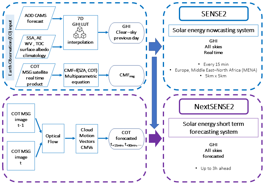
Figure 1Schematic overview of the solar energy nowcasting system (SENSE2) and system for short-term forecasting up to 3 h ahead (NextSENSE2).
The first improvements of the SENSE2 system are as follows:
-
The computations of clear-sky GHI are performed during the previous day for the whole domain (1.5 million pixels) every 15 min; for the current day, the real-time cloud information is applied to provide all-skies GHI in real time (no NN is used).
-
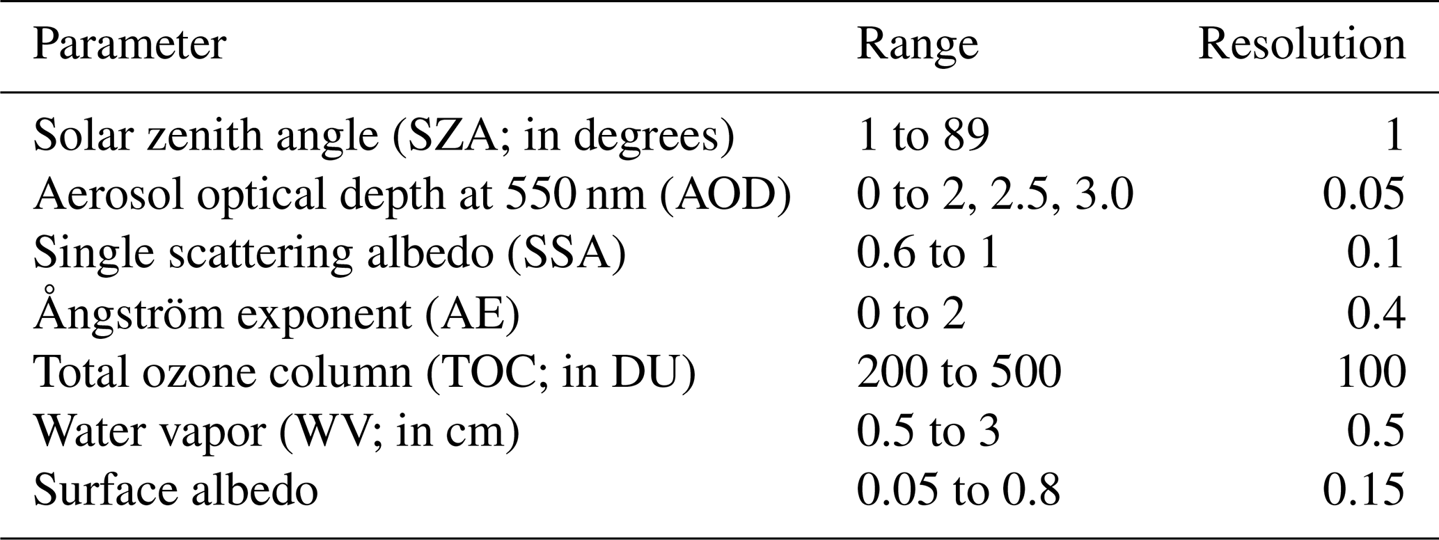
The computations of clear-sky GHI are based on a new, more-detailed LUT of ∼ 16 million combinations of simulated GHI at the earth's surface that was generated using the National Infrastructures for Research and Technology (GRNET) High Performance Computing Services and the computational resources of the ARIS GRNET infrastructure. The RTM simulations were performed using the libRadtran package (Emde et al., 2016; Mayer and Kylling, 2005). Table 1 summarizes the input variables and their resolution. The number of variables and their resolution resulted in a total of ∼ 16 million runs.
RTM simulations were performed spectrally from 280 to 3000 nm with 1 nm spectral resolution using the DISORT radiative transfer solver in pseudo-spherical mode (Buras et al., 2011). The molecular absorption parameterization of representative wavelength approach (REPTRAN; Gasteiger et al., 2014). was used to account for the absorption of atmospheric gases for the whole solar spectrum. The Kurucz 1.0 nm (Kurucz, 1994) extraterrestrial solar spectrum and the US Standard Atmosphere (Anderson et al., 1986) were used as inputs. The default aerosol model of Shettle (1989) was used as the basis, and the aerosol optical properties of AOD, single scattering albedo (SSA), and Ångström exponent (AE) were modified varying according to Table 1. The spectral global irradiances were integrated over the spectral range of the simulations to derive the GHI.
Table 1Input parameters for radiative transfer simulations performed on the ARIS GRNET supercomputer resulted to the 7D GHI LUT.
The clear-sky GHI estimates from SENSE2 (Fig. 1) are calculated on the previous day by linear interpolation in the seven dimensions (7D) of the precalculated GHI LUT using the corresponding inputs. Specifically, the solar zenith angle (SZA) values are precalculated for every grid cell of the domain (1.5 million in total) for 15 min time steps. The main input parameter for the clear-sky computations is the forecasted AOD at 550 nm from CAMS (“CAMS AOD” hereafter). The forecasts for the day of interest are values from the CAMS run initialized at 00:00 UTC on the previous day (e.g., the AOD used to simulate the GHI for the 24th of a month is derived from the CAMS run that started on the 23rd at 00:00 UTC). Climatological values are used for the interpolation in the 7D LUT for the additional aerosol optical properties SSA and AE (MAcv2 climatology; Kinne, 2019), the water vapor (WV) (CAMS reanalysis; Inness et al., 2019), the total ozone column (TOC) (climatological values based on ozone-monitoring instrument (OMI) TOC data; Bhartia, 2012), and the surface albedo (GOME-2 database of directionally dependent Lambertian-equivalent reflectivity; Tilstra et al., 2017, 2021). It should be mentioned that the interpolation procedure in the 7D LUT was added to the new SENSE2 to further improve the accuracy of the GHI estimations. Finally, since the results of the RTM runs are for sea level and the mean Earth–Sun distance, a post-correction of the clear-sky GHI values from the LUT is performed for the surface elevation using the methodology described in Fountoulakis et al. (2021) and the actual Earth–Sun distance for the particular day of year (DOY). Based on simulations for various atmospheric and surface albedo conditions, Fountoulakis et al. (2021) estimated an average increase of the GHI of 2 % per km, which has also been applied to the model output to correct the surface GHI for sites at higher altitudes than sea level.
The use of LUTs in operational surface solar radiation retrievals instead of direct RTM calculations is well established (e.g., Qu et al., 2017; Mueller et al., 2009). From a technical point of view, there are various concepts which can reduce the number of RTM simulations needed to generate a LUT by several orders of magnitude. Mueller et al. (2009) developed a flexible, fast, and accurate scheme to retrieve the broadband surface solar irradiance (CM CAF datasets) using the hybrid eigenvector approach, resulting in a combination of basis LUTs with an optimized interpolation grid and parameterizations using only almost 1000 RTM calculations. This approach was extended by Mueller et al. (2012) to wavelength bands for spectrally resolved surface solar irradiance retrievals from spaceborne data. This optimization of the computing performance is of paramount importance for the reprocessing of a large amount of satellite data (up to a few decades). In this work, the main concept behind the generation of our clear-sky LUT was to have spectral irradiance outputs (1 nm spectral resolution). The choice to calculate spectral solar data and not directly calculate total shortwave radiation is based on the fact that the SENSE2 output could be used for other applications (e.g., health and agriculture), based on the irradiance weighting of a relevant spectral range with an action spectrum (function) defined for each of the effects. So, a large number of RTM runs had to be performed (once) for the spectral surface solar irradiance that covered all possible combinations of atmospheric and surface states. Technically, since the operational setup of the SENSE2 model allows for the computation of the clear-sky GHI values from the previous day, the processing time for interpolation to the seven dimensions of the LUT has no effect on the timely production of the real-time output of the model every 15 min, while the accuracy of the clear-sky output is almost identical to direct RTM simulations (Papachristopoulou et al., 2022), and the uncertainties of the clear-sky GHI retrievals are related only to the uncertainties of the model inputs. In addition, this LUT includes various aspects, especially for aerosols (AOD, SSA, AE), that can reduce the uncertainty under different aerosol conditions for broadband solar radiation or specific spectral regions.
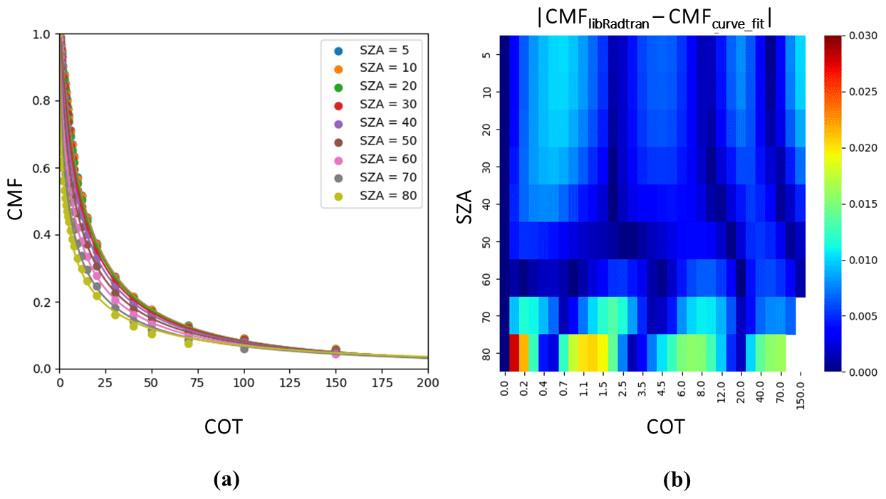
Figure 2(a) Cloud modification factor (CMF) versus cloud optical thickness (COT) and solar zenith angle (SZA) based on radiative transfer simulations of global horizontal irradiances using the libRadtran package. CMF is the ratio of the global horizontal irradiance (GHI) to the GHI under cloudless conditions (COT = 0). (b) Differences between the CMF derived directly from libRadtran simulations and that derived from Eq. (2) as a function of COT and SZA.
Another improvement is related to the cloud representation in real time using multi-parametric equations for different cloud scenes based on the cloud modification factor (CMF) concept instead of using the COT as an input parameter in direct RTM calculations. The computation of the all-skies GHI in real time every 15 min is based on the COT product we extract operationally in real time using broadcasted MSG satellite data and the software package provided by the EUMETSAT Satellite Application Facilities for Nowcasting and Very Short Range Forecasting, NWC SAF (Météo France, 2016; Derrien and Le Gléau, 2005). Neither the direct radiative transfer simulations nor the multi-dimensional interpolations would be sufficiently fast to provide the all-skies GHI SENSE2 product for 1.5 million pixels in a timely manner. Instead, a multi-parametric equation was constructed by fitting on libRadtran simulations for a wide range of COT values and different SZAs (see the points in Fig. 2a). The design of the cloud model was a trade-off between the relevance of the cloud property and the operational implementation of the model. It was shown in previous studies (Qu et al., 2017) that, in most of the cases (except for high surface albedo values > 0.9), the vertical position and extent of the cloud has only a small or a negligible influence on the RTM simulations of surface solar irradiance. Under cloudy conditions, COT is the variable that has the greatest impact on the simulation of surface solar radiation (Qu et al., 2017; Oumbe et al., 2014; Taylor et al., 2016). In our simulations, spherical droplets were assumed, with typical values for the effective radius (Reff = 10 µm) and typical climatological mean heights (cloud's base at 2 km and its height was 3 km) (Taylor et al., 2016; Kosmopoulos et al., 2018) used given the unavailability of height descriptors in the operational mode, the negligible influence of changes in droplet effective radius with respect to COT on the simulation of surface solar radiation (Oumbe, 2009), and that this setup helps to simplify the cloud model. The COT of the cloud layer at 550 nm is additionally specified, which leads to an adjustment of the default liquid water content value of 1 g cm−3 using the parameterization from Hu and Stamnes (1993). Finally, homogeneous cloud layer was used for the libRadtran simulations, meaning a cloud cover fraction value of 100 %, which is one of the model's limitations, since it is not always correct to assume totally cloudy pixels for low values of COT (Mueller et al., 2009). The simulated GHI for each COT was divided by the GHI for COT = 0 (clear sky) for the same SZA to derive the CMF (Eq. 1). The CMF ranges from 0 (overcast conditions) to 1 (clear sky) and is easy to use to provide all-skies GHI by simply multiplying the clear-sky GHI by CMF (Eq. 3). The libRadtran-derived CMFs for each SZA were fitted against COT using a hyperbolic tangent function. The resulting fits are shown as solid lines in Fig. 2a and are mathematically expressed by the multi-parametric Eq. (2).
Here, a and b are polynomials of SZA:
The real-time MSG COT is used, along with SZA, as an input in Eq. (2) every 15 min for ∼ 1.5 million pixels to calculate the CMF (“CMFmsg” hereafter). Apart from being very fast, this formula also accurately calculates CMFmsg, as can be seen by a comparison of the CMF values derived by Eq. (2) against those from libRadtran runs (Fig. 2b). CMF differences are less than 0.015 (or 1.5 %) for SZAs lower than 70°, while they are up to 0.03 (3 %) for SZAs between 80 and 90°, showing the very good representation of the CMF as a function of COT achieved with Eq. (2). In terms of accuracy, this means that using Eq. (2) is almost the same as running RTM simulations, but in terms of computational time, Eq. (2) is far more efficient in the operational mode. Finally, by multiplying CMFmsg by the clear-sky GHI, the all-skies GHI product is obtained (Eq. 3) in less than 1 min for 1.5 million pixels.
The new SENSE2 configuration was built to improve GHI nowcasting at the 15 min timescale. Additionally, it allows the system greater flexibility:
-
It can include reanalysis or measured data of AOD and other optical properties, e.g., CAMS reanalysis or AERONET measurements.
-
It can be extended to other output products. Apart from GHI, the direct normal irradiance (DNI) or total irradiance on a tilted surface could be also produced. By introducing spectral information and making the appropriate modifications, products related to specific spectral regions could also be derived (e.g., the UV index (using real-time TOC data as input) and the photosynthetically active radiation (PAR)).
-
It can run a past time series for one or a few locations autonomously using actual measurements as input. In this case, if there is no time constraint, model runs could be performed without the parameterizations (LUT and multi-parametric functions).
2.2 NextSENSE2
NextSENSE2 is the operational system that provides forecasts of GHI up to 3 h ahead with a 15 min time step by applying a CMV technique to the MSG COT product (Fig. 1). In this section, we describe the method employed to produce forecasted COT, which is the main input used to derive the operational forecasts of GHI. All the other EO inputs and the radiative transfer parameterizations for fast estimates of forecasted GHI are the same as those described in the previous section for the SENSE2 model.
We use CMVs to predict the motions of the clouds and project their future positions. The CMVs in NextSENSE2 are calculated by applying a state-of-the-art optical flow algorithm from the computer vision community. Optical flow is the apparent motion of objects between consecutive frames, which is caused by the relative movement between the object and a camera. We apply the Farnebäck (2003) two-frame motion estimation technique to images of the COT product (Kosmopoulos et al., 2020). Several other optical flow algorithms, like TV-L1, are available as free software (OpenCV) and are used for cloud motion estimation in solar energy short-term forecasting systems (Urbich et al., 2019). In this study, we used the Farnebäck technique based on the results of a previous study by Kosmopoulos et al. (2020). The optical flow displacement vectors are calculated by applying the algorithm to two consecutive images of satellite-derived COT. This CMV field is applied to the later COT image (real) to get the next COT image (forecasted COT). This procedure is performed 12 times, resulting in the 3 h forecasting horizon. The main assumptions are brightness constancy and that the cloud's displacements are only two-dimensional (i.e., in the image plane). More details regarding the CMV model and forecasted COT can be found in Kosmopoulos et al. (2020).
2.3 Persistence forecast
It is not easy to evaluate the quality of different forecasting methods of surface solar radiation using only statistical metrics, since the study period, the geographical area, and other factors affect their forecasting accuracies. That is why it is a typical evaluation practice to benchmark the different forecasts against some simple forecast methods (Pelland et al., 2013). We used the persistence forecast to benchmark the CMV-forecasted GHI of the NextSENSE2 system, which is a commonly used reference in solar forecasting (e.g., Kosmopoulos et al., 2020; Kallio-Myers et al., 2020). This method assumes that the state of the clouds remains constant for future time steps, while all other variables, like SZA, dynamically change. Hence, it uses the same COT values from the later satellite information as input to the next 12 time steps in order to forecast the GHI up to 3 h ahead.
2.4 Ground-based irradiance measurements
To validate the modeled GHI, ground-based measurements from pyranometers were utilized. The ground-based 1 min GHI measurements were collected from stations of the Baseline Surface Radiation Network (BSRN; Driemel et al., 2018), which are within the study area and have data for all of 2017, and from two additional stations at Athens (ASNOA: the NOA's Actinometric Station) and Thessaloniki. Table 2 summarizes information on all 10 stations utilized, and Fig. 3 depicts their geographical locations.
Table 2Detailed information about the ground-based stations used in this study.
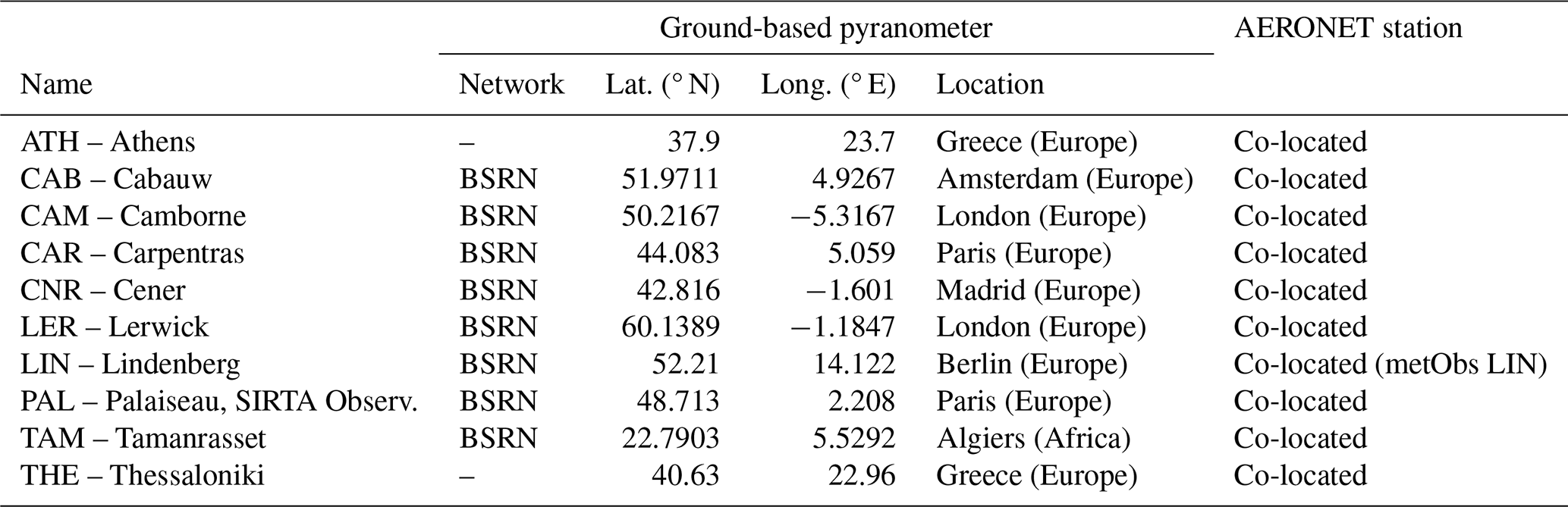
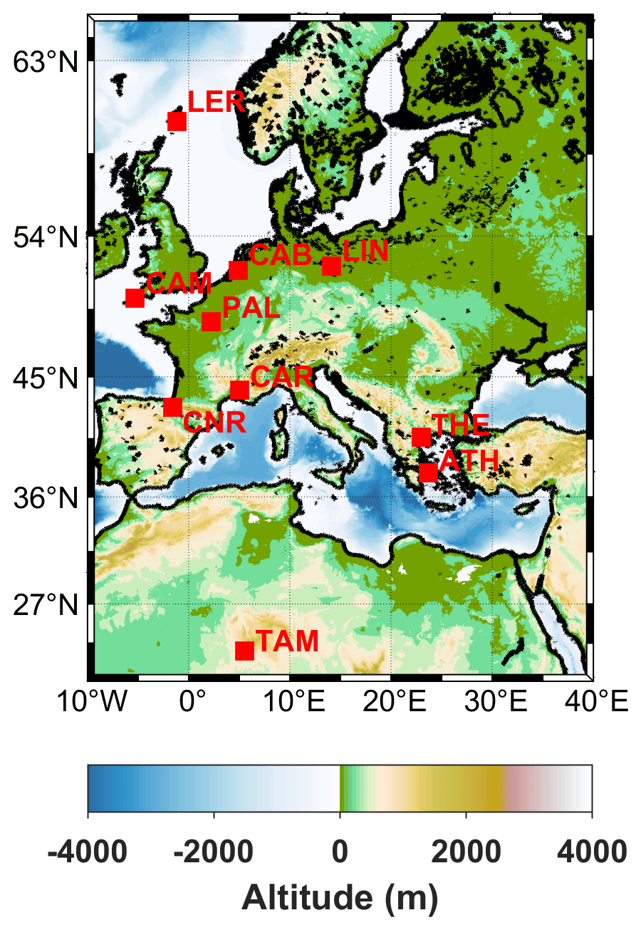
Figure 3Locations of the ground-based stations measuring global horizontal irradiance (GHI) that are used in the current study. These are eight BSRN stations plus Athens and Thessaloniki in Greece.
BSRN station-to-archive files were accessed and manipulated using the SolarData v1.1 R package (Yang, 2019). The function that reads the data from the station-to-archive files also computes several auxiliary variables, such as solar zenith angle, clear sky irradiances using the Ineichen–Perez clear-sky model (Ineichen and Perez, 2002), and extraterrestrial GHI. Using the same methodology, the Ineichen–Perez clear sky model values were also computed for the non-BSRN station data by adjusting the functions of the SolarData v1.1 R package for the non-BSRN stations.
The BSRN-recommended quality check (QC) tests (Long and Dutton, 2010) were applied to the collected measurements to ensure that they were of the best quality. Measurements that did not pass the above QC tests were flagged and labeled as missing values. The GHI records that are available at the two Greek stations (1951–present in Athens; 1993–present in Thessaloniki) are among the longest continuous high-quality GHI records in the eastern Mediterranean Basin, an area where BSRN data are not available for the period of this study. The pyranometers in Athens and Thessaloniki are calibrated regularly, and the GHI measurements were subjected to quality control before being used in the study. More information on the GHI datasets for the Thessaloniki and Athens stations can be found in Bais et al. (2013) and Kazadzis et al. (2018), respectively.
2.5 Ground-based aerosol information
To assess the CAMS AOD forecasts used as input to the model, ground-based measurements of AOD from the AERONET network (Holben et al., 1998) were used. Each of the ground-based stations with pyranometer data (BSRN, Athens, and Thessaloniki) has a collocated AERONET station (see Table 2). The level 2, version 3 direct sun (Giles et al., 2019) AOD data at 500 nm were collected and the AOD values at 550 nm were derived using the Ångström exponent for 440–675 nm. However, measurements of AOD at 500 nm were not available for Cabauw, so the AOD at 440 nm was used instead and converted to 550 nm using the Ångström exponent for 440–675 nm.
2.6 Evaluation metrics
Common statistical metrics were adopted for the validation of the SENSE2- or NextSENSE2-derived GHI values against ground-based measurements. Given that the error is defined as the difference between the modeled values (xm_i) and the observed values (xo_i), we have three common metrics: the mean bias error (MBE), root mean square error (RMSE), and Pearson correlation coefficient (R).
The relative values of the latter two metrics, rMBE and rRMSE, were obtained with respect to the mean of the observed values of GHI.
An additional metric, the forecast skill (FS), was used to assess the performance of CMV-forecasted GHI using the persistence model as a benchmark model:
where rRMSECMV and rRMSEpers are the relative RMSEs of the CMV and persistence forecasting models, respectively.
The results are discussed separately for the evaluation of nowcasted GHI (Sect. 3.1) based on SENSE2 outputs (“modeled GHI” hereafter) and the evaluation of the short-term forecasted GHI (Sect. 3.2), namely the NextSENSE2 product (“forecasted GHI” hereafter). The comparisons between ground-based and estimated GHI were restricted to SZAs below 75° (i.e., for solar heights above 15° from the local horizon) because the accuracy of satellite cloud retrievals is degraded for higher SZAs.
The CMF derived from the ground-based measurements of GHI was used in our analysis to evaluate CMFmsg and to categorize the cloudiness conditions. Specifically, the CMF was calculated as the ratio (Eq. 7) of the measured GHI to the clear-sky irradiance calculated by the Ineichen–Perez clear-sky model (Ineichen and Perez, 2002) (see Sect. 2.4):
Three categories of CMF are considered in the following: CMF ≥ 0.9 for clear-sky conditions, 0.4 < CMF < 0.9 for partially cloudy conditions, and CMF ≤ 0.4 for overcast conditions.
3.1 Nowcasting
3.1.1 Overall performance
Figure 4 presents the overall performance of the SENSE2 system at the (instantaneous) 15 min timescale by comparing the modeled GHI values against ground-based measurements from all stations for a whole year (2017). We can see that most of the points (Fig. 4a; number of cases N > 600) fall on the 1 : 1 line (blue line), which indicates that the system shows good performance overall, with a correlation coefficient of 0.93. For 58 % of the cases, the absolute differences between modeled and ground-based measurements of GHI are within ±50 W m−2 or ± 10 % (Fig. 4b). The SENSE2 system mostly overestimates the GHI, leading to points above the identity line (Fig. 4a; MBE is 23.8 W m−2 (4.9 %)); this overestimation is more pronounced for low irradiances (lower-left corner of Fig. 4a where GHI < 250 W m−2). Lerwick is the most northern station and also the station with the greatest MBE (Fig. 4b and Figs. A1, A2 in Appendix A).
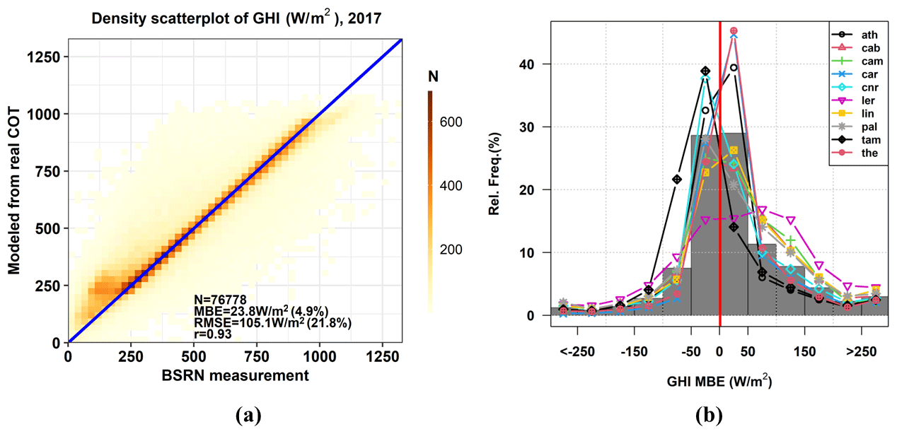
Figure 4(a) Comparison of the modeled versus measured global horizontal irradiance (GHI) for all ground-based stations in 2017. (b) Relative frequency of GHI MBE for all stations (gray bars) and for each station (lines with different symbols and colors).
We investigated how the mean cloudiness (CMF) of every station, the station's latitude, and the mean measured GHI influenced the GHI MBE; the results are presented in Fig. 5. The GHI MBE increases with an increase in cloudiness (a decrease in mean CMF). At the same time, the cloudiness increases and lower values of mean measured GHI are observed with increasing latitude. Those results are in line with previous studies (Qu et al., 2014, 2017). According to Qu et al. (2014), the error of the satellite estimates of surface solar radiation increases with an increase in the distance from the subsatellite point (lat = 0°, long = 0° for Meteosat) and an increase in the occurrence of fragmented cloud cover. Qu et al. (2017) found that their retrievals for the northernmost stations were less accurate, which was attributed to the more frequent cloud occurrence over those stations and the more erroneous satellite retrievals of cloud properties for large SZAs and satellite viewing angles. One of those stations was Lerwick, which is close to the edge of the field of view of the Meteosat satellite, where errors due to parallax become important (Marie-Joseph et al., 2013; Schroedter-Homscheidt et al., 2022). The effect of clouds on GHI estimates is investigated in more detail in Sect. 3.1.3.
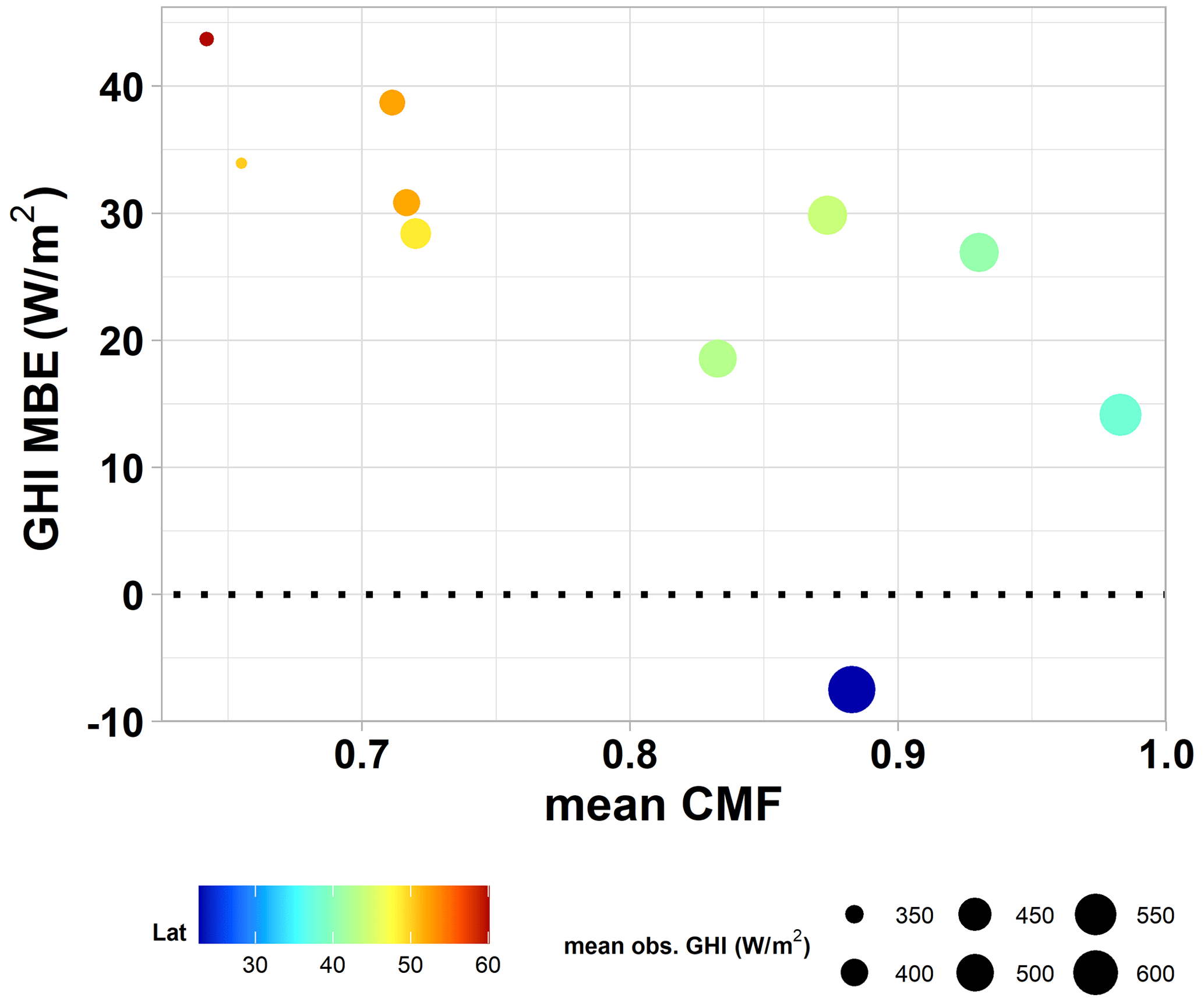
Figure 5Dependence of the GHI MBE on the mean CMF for all stations. The color of each point indicates the latitude of the station and its size indicates the magnitude of the mean GHI observed at the ground-based station.
All the statistical metrics are drastically improved by increasing the timescale for all stations (Fig. 6). The northernmost stations (CAB, CAM, LER, LIN, and PAL) show similar results. At the 15 min timescale, the MBE, RMSE, and correlation coefficient show ranges of 29–43 W m−2, 104–131 W m−2, and 0.82–0.90, respectively. Those statistics are improved for the monthly means to 5–10 W m−2 for MBE, 7–13 W m−2 for RMSE, and R ∼ 1. Similar results were found for the rest of the stations (which are the southernmost ones): the MBE, RMSE, and correlation coefficient range from −7 to 30 W m−2, from 84 to 104 W m−2, and from 0.93 to 0.95, respectively, for the 15 min timescale, whereas the MBE ranges from −4 to 8 W m−2, the RMSE ranges from 6 to 10 W m−2, and R ∼ 1 for monthly means. The overall MBE and RMSE are reduced to 6.6 W m−2 (3.3 %) and 15.4 W m−2 (7.7 %) for the daily mean GHI and to 5.7 W m−2 (3.2 %) and 9.2 W m−2 (5.2 %) for the monthly means, while the correlation coefficient shows values that almost reach 1, which was anticipated since the cloud effect is smoothed out for larger timescales.
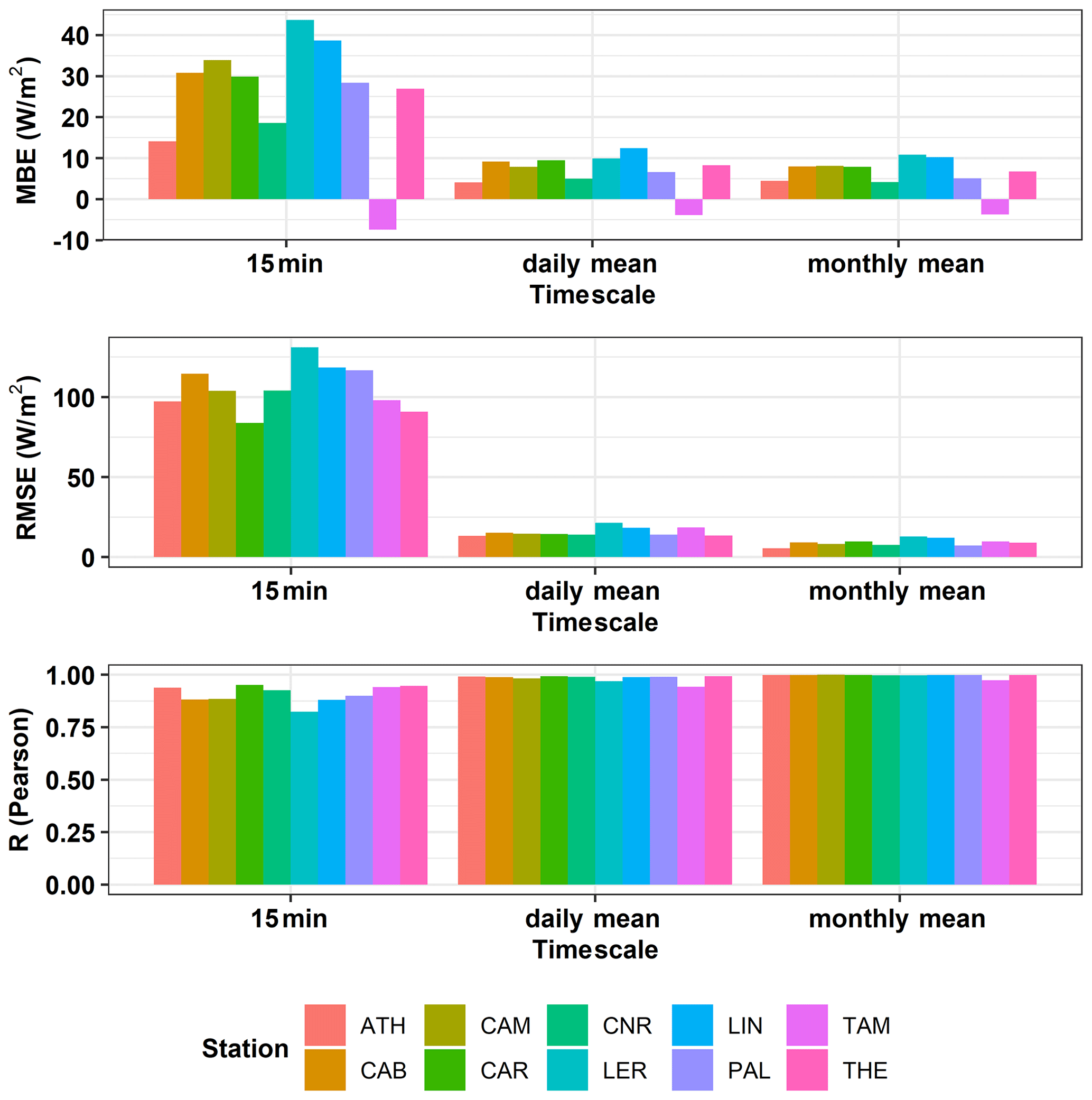
Figure 6Comparison of the modeled versus measured global horizontal irradiance (GHI) per ground-based station in 2017 for different timescales (15 min, daily mean, and monthly mean).
3.1.2 Aerosol effect on the retrieved solar irradiance
The CAMS AOD forecasts used as input to the operational model were assessed against ground-based measurements from the AERONET network, and the related uncertainty introduced into the modeled GHI was calculated. The AERONET AOD direct sun measurements were matched with CAMS AOD forecasts (1 h time resolution) interpolated to the 15 min time steps of the model. The closest AERONET measurement ±10 min around each 15 min time step was matched (or the mean value was used if more than one measurement was available). To estimate the model uncertainties due to the forecasted AOD, the clear-sky GHI was calculated using the forecasted CAMS AOD and the synchronized AERONET AOD measurements as input. The MBE for AOD (CAMS against AERONET) and clear-sky GHI (modeled using CAMS AOD against those using AERONET AOD) per station is presented in Fig. 7.
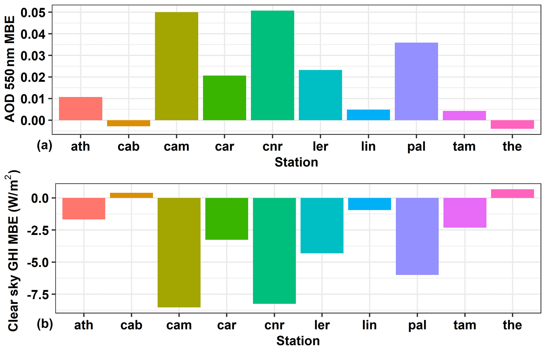
Figure 7(a) Mean bias error (MBE) of the aerosol optical depth (AOD) at 550 nm forecasted by CAMS (1 d ahead forecast) compared to the AOD measured by ground-based sun photometers of the AERONET network. (b) MBE of global horizontal irradiance (GHI) modeled under clear-sky conditions using the CAMS-forecasted AOD at 550 nm as input versus measured values (AERONET).
CAMS forecasts mostly overestimate AOD, with an MBE of 0.015 (10 %) for all stations, which results in an underestimation of the modeled clear-sky GHI of −2.7 W m−2 (−0.4 %). The greatest overestimation, 0.05 (∼ 50 %), was found for CAM and CNR; this resulted in the greatest underestimation of modeled clear-sky irradiance: −8.5 W m−2 (−1.4 %). An underestimation of AOD was found for CAB and THE, with an MBE of < 0.01 (< 3 %), resulting in negligible overestimation of the modeled irradiance (MBE < 1 W m−2 or 1 %).
An overestimation of the CAMS-forecasted AOD at 550 nm for 2017 over Europe is also reported (the average modified normalized mean bias ranges from ∼ 10 % to 30 %), which is based on the continuous quarterly evaluation of the AOD forecasts against daily AERONET cloud-screened (i.e., version 3, level 1.5) sun photometer data (Basart et al., 2023; Eskes et al., 2021). While this is the case on average, in contrast, the CAMS-forecasted AOD is underestimated during high aerosol loads, especially in desert regions and during dust events (Basart et al., 2023; Papachristopoulou et al., 2022), which might explain the almost zero bias for Tamanrasset station (the overestimation of small AODs is masked by the frequent underestimation of large AODs) compared to the greater values of bias (> 0.01) found for most of the other stations. Qu et al. (2017) analyzed case studies at Tamanrasset and found that the CAMS (MACC) AOD at 550 nm is frequently found to be underestimated when compared against AERONET data during summer dust events, explaining the strong positive bias they found for their modeled direct irradiance (using the Heliosat-4 method and the McClear clear-sky model). In the same study (Qu et al., 2017), in contrast to the CAMS AOD underestimation that occurred during dust events, a systematic overestimation of AOD during periods free of those events was found for the two desert stations examined (Sede Boqer and Tamanrasset) which the study linked to an underestimation of the modeled direct irradiance at those stations. The updated McClear v3 clear-sky model was used in the study by Schroedter-Homscheidt et al. (2022), and a negative bias was found for their GHI estimates under clear-sky conditions for most of the stations, especially those located in dust-affected regions, which is in line with our results – although the results are not directly comparable since they performed a direct comparison with the BRSN-measured irradiances. Our results demonstrate that the clear-sky model using CAMS forecasts shows good performance, highlighting that the AOD product forecasted by CAMS is suitable for GHI-nowcasting applications.
3.1.3 Cloud effects on the retrieved solar irradiance
Overall, the model overestimates GHI, as we saw in Sect. 3.1.1. The improvement of the statistics upon going from an instantaneous comparison to integrated timescales (e.g., daily) indicates that this overestimation can be attributed to the uncertainties related to the cloud information from satellite retrievals but also to satellite/ground-based evaluation representativity issues. In order to understand this more closely, we investigated the effect of different conditions in cloudiness on the error in the modeled GHI.
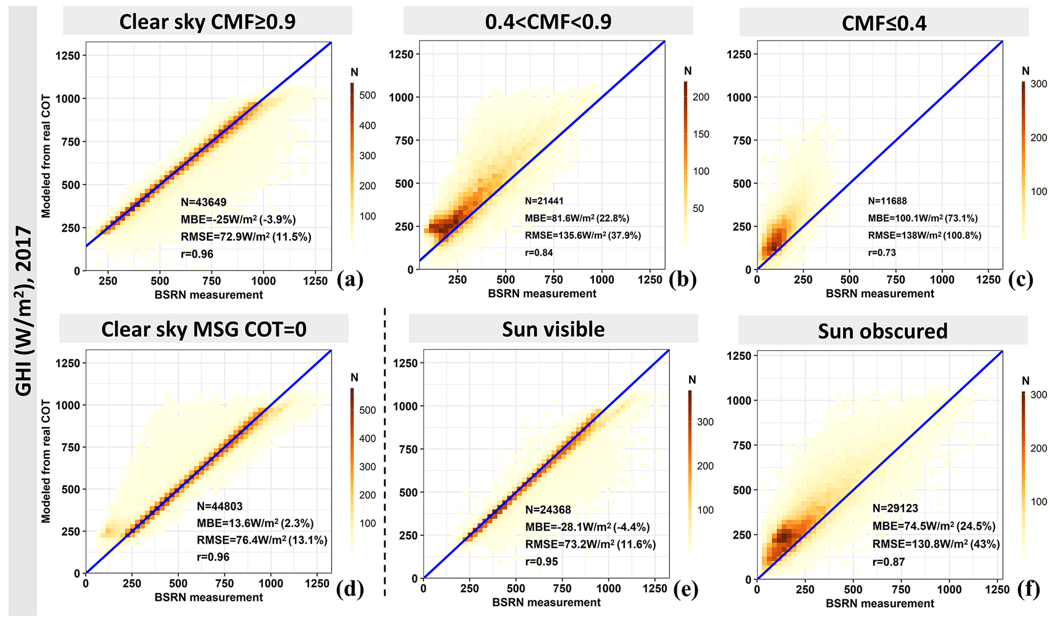
Figure 8Comparisons of the modeled versus the measured global horizontal irradiance (GHI) at all ground-based stations (a–c) for different cloudiness conditions based on the cloud modification factor (CMF; the ratio of ground-based GHI measurements to clear-sky GHI (clear-sky model)), (d) for clear-sky conditions as determined by the MSG satellite product for zero cloud optical thickness (COT = 0), and (e, f) for conditions characterized as “sun visible” or “sun obscured” over the ground-based station.
Initially, we classified the cloudiness conditions using the ground-based CMF (Fig. 8a, b, c). According to the results, GHI is overestimated by the model under cloudy conditions (CMF < 0.9), while for clear-sky conditions (CMF ≥ 0.9, Fig. 8a), the model closely resembles the measured GHI. For partially cloudy conditions (0.4 < CMF < 0.9, Fig. 8b), the MBE is 81.6 W m−2 (22.8 %) and the greatest error in GHI occurs for low CMF values (CMF ≤ 0.4, Fig. 8c) (MBE = 100.1 W m−2 or 73.1 %). High deviations at low measured GHI values (< 250 W m−2) are most commonly found in the latter category.
We also compared the modeled and measured GHI values for clear-sky conditions according to the satellite data, namely for COT = 0 (Fig. 8d). In this case, the model overestimates GHI, with an MBE of 13.6 W m−2 (2.3 %). Most of the cases are on the 1 : 1 line, with a few being higher, especially for measured GHI < 250 W m−2, meaning that there are clouds over the ground-based station that have not been resolved by the satellite pixel (COT = 0). A positive bias was also found at all stations examined by Qu et al. (2017) for clear-sky pixels as defined by the APOLLO/SEV cloud properties retrieval scheme, which contributed to the overall overestimation for all skies. This was attributed to small broken clouds that cause large variability in surface GHI and to false detections by the cloud retrieval algorithm being treated as clear-sky cases.
To demonstrate the effect of sun visibility over the ground-based stations on the GHI error, we tried to separate out those instances by using the pyrheliometer measurements of direct irradiance (DNI – direct normal irradiance) available from the BSRN network. The DNI measurements (1 min) were divided by the clear-sky DNI, which was again obtained from the Ineichen–Perez clear-sky model (Ineichen and Perez, 2002). We classified situations with a ratio of actual to clear-sky model DNI of > 0.8 as “sun visible”. This threshold was selected to account for the strong effect of aerosols on DNI, given that a monthly mean climatological value for the aerosol attenuation factor is used by the DNI clear-sky model (Ineichen and Perez, 2002). We classified situations with a ratio of < 0.6 as “sun obscured”, and we omitted situations with ratio values between 0.6 and 0.8 (“unclassified situations”) so that we could be confident by more than 40% that the direct irradiance was blocked by clouds. The results of the comparison between modeled and measured GHI values were grouped based on the sun visibility classification and are presented in Fig. 8e and f. We can see that the sun-visible situations give quite good results (points close to the 1 : 1 line, with an MBE of −28.1 W m−2 or −4.4 %).
In contrast, the model overestimates GHI (MBE is 74.5 W m−2 or 24.5 %) when the sun is obscured over the ground-based station. Comparing Fig. 8b and c with Fig. 8f, we can see that most of the cases that are above the 1 : 1 line happened when the sun was obscured. This is caused by the fact that the satellite-based cloud retrieval is representative of the whole pixel, while the information on whether the sun is obscured over the ground-based station is representative of the (point) station and cannot be inferred from the satellite cloud retrievals. This – combined with the facts that the direct irradiance attenuation from clouds is completely different from GHI, it does not linearly decrease with cloudiness or cloud optical thickness, and, finally, its contribution to GHI depends on various parameters (mainly the solar elevation) – introduces an issue into any instantaneous comparison between a satellite-based GHI retrieval representing a whole pixel and a GHI value measured at a single point. So, the main result of this analysis of sun visibility over a station is to discuss possible systematic biases due to the satellite pixel versus station evaluation representativeness issue. This issue makes instantaneous model output evaluation difficult, especially in partly cloudy situations.
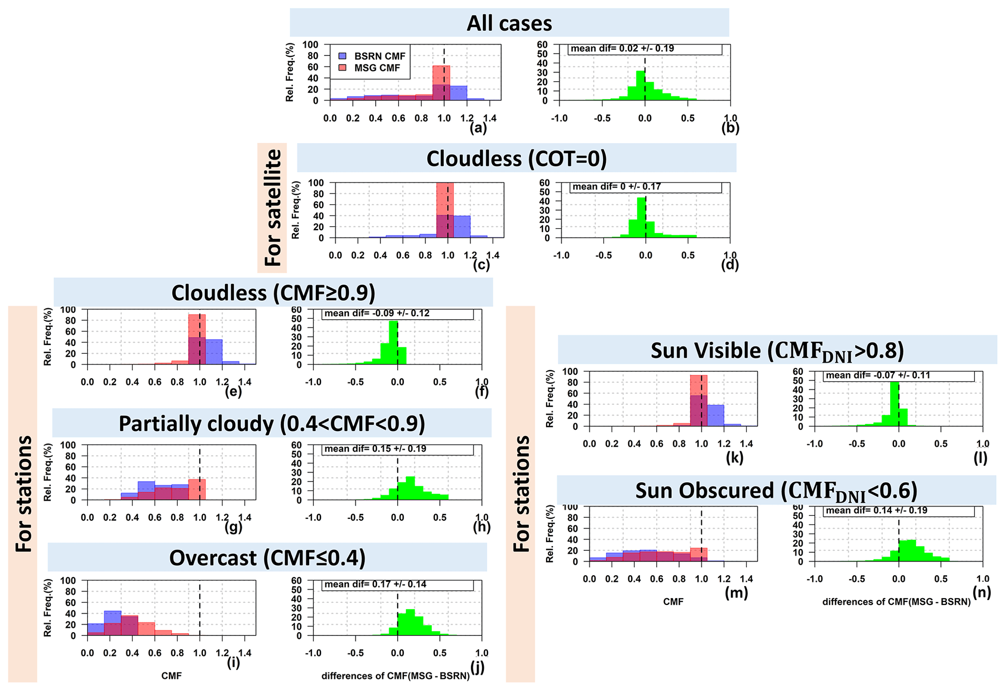
Figure 9Left panels (a, c, e, g, i, k, m): distributions of the cloud modification factors (CMFs) from measurements of global horizontal irradiance (GHI) (blue bars) and from the MSG cloud optical thickness (COT) (red bars) for all cases and under different cloudiness conditions. Right panels (b, d, f, h, j, l, n): distributions of the difference between the CMF derived from MSG satellite COT against the CMF derived from measurements of GHI.
Since the main source of errors in this analysis is associated with clouds, we further assessed the satellite-derived cloud input in the model. The MSG COT is transformed into CMFmsg using Eq. (2), and this is the cloud-related input in the SENSE2 model. Since this cannot be evaluated directly with ground-based measurements, we indirectly evaluated CMFmsg with the CMF derived from GHI measurements (Eq. 7). The results are presented in Fig. 9 as relative frequency distributions of CMFmsg, CMF, and the difference between them (CMFmsg – CMF) for all cases and different cloudiness conditions. Overall, the CMFmsg is overestimated (0.02; Fig. 9a and b), which is the reason for the overestimation of SENSE2-modeled GHI overall. This CMFmsg overestimation occurs mainly when there are cloudy conditions (Fig. 9g, h, i, and j) and where the sun is obscured over the ground-based station (Fig. 9m and n).
There are also cases of CMFmsg underestimation (CMF differences < 0 in Fig. 9b), which come mostly from situations characterized as cloudless (CMF ≥ 0.9, Fig. 9e and f) and explain the points below the 1 : 1 line in Figs. 4a and 8 (i.e., those for which the measured GHI is greater than the modeled one). The first reason for this is a cloudy satellite pixel (corresponding to CFMmsg < 1 in Fig. 9e) but a ground-based CMF = 1 (which indicates that no clouds are present over the station). There are also many cases where CMF > 1 (Fig. 9e) that is attributed to irradiance enhancement by clouds, which often occurs when the sky above the ground station is partially cloudy but the sun is visible (see also Figs. 9k and l and 8e). In this case, the reflection of solar radiation by clouds increases the diffuse component from directions relatively close to the sun, hence the measured GHI on the ground. This is a three-dimensional effect of clouds that cannot be reproduced using the one-dimensional radiative transfer modeling used in this study. This is a limitation of the SENSE2 model – it does not include three-dimensional cloud effects (enhancement of the GHI or parallax) which can be reproduced using 3D RT simulations (e.g., Mayer, 2009). However, three-dimensional cloud structure information is not available for an operational solar energy nowcasting model from geostationary satellites (Qu et al., 2017; Schroedter-Homscheidt et al., 2022); besides, the introduction of parameterizations and techniques to improve the computational time (Tijhuis et al., 2023) is essential.
Summarizing, to explain the overestimation of SENSE2 GHI retrievals, we have to recognize that a direct comparison between point measurements of solar radiation at the ground and satellite estimates representative of a pixel introduces deviations (e.g., Kazadzis et al., 2009; Schenziger et al., 2023; Carpentieri et al., 2023) that are linked with the cloud features within the pixel and the limitations of cloud monitoring using satellite data (e.g., spatial resolution). We investigated the distributions of both CMFs and the differences between the CMFs separately for, again, clear-sky conditions according to the satellite (namely COT = 0; Fig. 9c and d). Regardless of the fact that CMFmsg can only be one, meaning that no clouds are resolved by the satellite, there are cloudy cases with CMF < 1 for the ground-based station (Fig. 9c). Due to the satellite's spatial resolution, small-scale broken clouds cannot be resolved in some cases (e.g., Schenziger et al., 2023; Marie-Joseph et al., 2013; Qu et al., 2017), but those clouds may have a significant impact on the ground-based measured irradiance if they are obscuring the sun (almost total attenuation of the direct irradiance). If they do not obscure the sun, this also corresponds to the clear-sky case for the ground-based station, although the effect of cloud enhancement of the measured GHI cannot be excluded (CMF = 1 and CMF > 1 in Fig. 9c, respectively). In a recent study by Schenziger et al. (2023) using sky camera images, the limitation of MSG satellite-based modeled CMF was demonstrated for small-scale clouds. Different results were obtained for two different stations inside the same satellite pixel, which was characterized as cloud free. For one station that was cloud free, the model agreed with the measurements; however, for the station that was covered by localized cumulus clouds that could not be resolved by the satellite, there were discrepancies between the ground-based and satellite-based modeled values. Nevertheless, even for the cases where the satellite imager can resolve clouds within a partially cloudy pixel, the COT product for this pixel is a constant value, namely a spatially homogeneous cloud optical property for the corresponding area. In this atmospheric scene with a high spatial variability of clouds, the results of the comparison will depend dramatically on whether the GHI is measured at ground level with the sun obscured or unobscured.
3.1.4 Bias correction based on the cloud input
Overall, the model overestimates GHI, which is attributed to the CMFmsg overestimation. Based on the main conclusions from the investigation of CMF differences in the previous section, we tried to find out if there is a pattern for CMF difference (modeled against measured) as a function of CMFmsg that is common to all stations, since it is the only operationally available input every 15 min. Additionally, we found that those differences hardly change with SZA (Fig. B1 in the Appendix B), so we only investigated their relationship with CMFmsg.
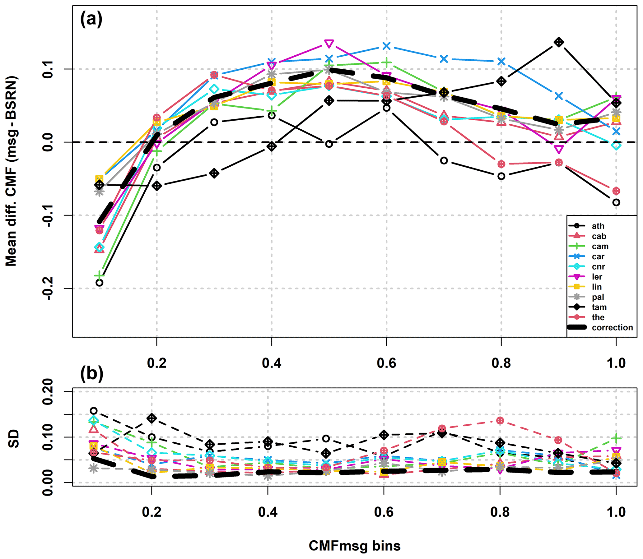
Figure 10(a) Mean differences between cloud modification factor (CMF) modeled from MSG satellite cloud optical thickness values (CMFmsg) and CMF derived from global horizontal irradiance (GHI) measurements per modeled CMFmsg bin. (b) The corresponding standard deviations (SDs) of the CMF differences per modeled CMFmsg bin. Lines with different colors and different symbols correspond to different stations.
We calculated the mean CMF difference and its standard deviation per CMFmsg bin for every station, and the results are presented in Fig. 10. A pattern of mean CMF differences in which the CFMmsg overestimation reached almost 0.1 starting at CMFmsg bin 0.3 and continuing up to bin 0.8 was found for almost all stations (apart from TAM, ATH ,and THE), which was also related to the low standard deviations in those bins.
As we discussed in the previous section, this CFMmsg overestimation (up to ∼ 0.1) is mostly related to partial cloudiness and sun-obscured conditions over the station. Nevertheless, the sun's visibility above a station is an information that cannot be provided by satellites. Consequently, we tried to correct CMFmsg (the operational input) with the CMF differences (modeled against measured values). We used the mean of the CMF differences per CMFmsg bin from 7 out of 10 stations (excluding TAM, ATH, and THE) to derive the correction factor (“the correction” hereafter), which is depicted as a dashed thick black line in Fig. 10. The correction was only applied to CMFmsg values in bins 0.3–0.8. The correction was applied to all stations, including TAM, ATH, and THE, which acted as a test bed (with a low frequency of cloudy cases) for the general correction derived from the other seven stations.
Table 3 summarizes the statistics of the corrected modeled GHI against ground-based measurements. The MBE and RMSE are improved after the correction. LER and CAM are the two stations with the greatest improvements in their statistics, followed by CAB and LIN, which was anticipated since those stations are at higher latitudes (associated with high cloudiness). Even stations ATH and THE, which were not used in the correction factor derivation, exhibit better results after applying the correction. TAM is the only station for which the statistics were not improved. Because cloudiness was rare at that station, its statistics were already good, indicating that a hybrid approach to the correction based on the area's cloudiness would probably be better. Overall, after the correction, the GHI differences (modeled against measured values) were within ±50 W m−2 (or ±10 %) for 61 % of the cases. The MBE for all stations was also improved to 11.3 W m−2 (2.3 %) compared to the uncorrected value (23.8 W m−2 or 4.9 %). For the daily mean GHI, the overall MBE and RMSE were improved to 3.3 W m−2 (1.7 %) and 13.1 W m−2 (6.6 %) compared to the uncorrected values of 6.6 W m−2 (3.3 %) and 15.4 W m−2 (7.7 %), respectively. For monthly means, the MBE improved to 2.7 W m−2 (1.6 %) compared to 5.7 W m−2 (3.2 %) before correction, and the RMSE improved to 6.3 W m−2 or 3.6 % (it was 9.2 W m−2 or 5.2 % before correction).
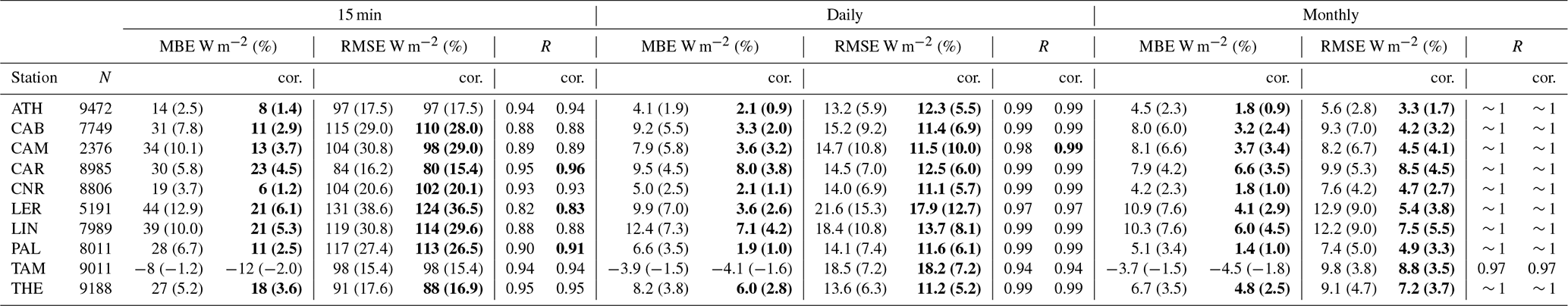
Table 3Performance of nowcasted irradiances before and after correction with CMFmsg. “cor.” indicates corrected values; those that were improved after the correction are shown in bold.
After improving the configuration of the SENSE2 model and correcting the bias in CMFmsg for partially cloudy conditions (the “bell-shaped curve” between CMFmsg bins 0.3 and 0.8, which has been also reported in other studies, e.g., Marie-Joseph et al., 2013), more accurate estimates of GHI were produced, in line with the results from similar models (Qu et al., 2014; Thomas et al., 2016; Qu et al., 2017). These SENSE2 GHI estimates will be the basis for the new forecasting system NextSENSE2 evaluated in the next section (Sect. 3.2).
Comparing our results with other studies, for the HC3v3 database of surface solar irradiation (Qu et al., 2014), correlation coefficient values greater than 0.92 and relative RMSEs between 14 %–38 % were found for the 15 min timescale. In the same study, for daily irradiation, correlation coefficient values greater than 0.97 were found, along with relative RMSEs between 6 % and 20 %. For the latest version (5) of HelioClim-3 database (HC3v5), validation against 14 BSRN stations (Thomas et al., 2016) resulted in relative biases between −4 % and 5 % and rRMSEs between 14.1 % and 37.2 % for GHI. Both studies highlight the good performance of the clear-sky irradiation values from the McClear clear-sky model (which uses advanced inputs for aerosol, water vapor, and ozone instead of climatological values). A comparison of the 15 min means of global irradiance estimated by the fully physical Heliosat-4 method (a combination of the McClear and McCloud models) against ground-based measurements from 13 stations of the BSRN network (Qu et al., 2017) showed large correlation coefficients for all stations (0.91–0.97) and biases and RMSEs of GHI that ranged between 2–32 and between 74–94 W m−2, respectively. In the same study, the greatest values of the relative RMSE of the mean irradiance were found for stations with rainy climates and mild winters (26 % to 43 %, with the greatest value found for the northernmost station), while values for stations in desert and Mediterranean climates ranged between 15 % and 20 %, which are in line with our findings for the northernmost and southernmost stations, respectively, in this study. The positive biases previously observed when using the APOLLO cloud retrieval in Heliosat-4 (Qu et al., 2017) for the CAMS Radiation Service were significantly reduced and balanced after applying the new cloud retrieval scheme APOLLO_NG (a new cloud mask with a cloud probability threshold of 1 %, among other improvements; for more details, see Schroedter-Homscheidt et al., 2022). After the improvements, relative RMSE values of hourly GHI of between 10.3 % and 25.5 %, along with a mean value of 13.7 %, were reported for 2015 (Schroedter-Homscheidt et al., 2022). An extensive validation (Urraca et al., 2017) of the operational radiation product (ICDR) of the CM SAF over Europe for the 2008–2015 period gave an MBE of 4.5 W m−2 (4 %) and an RMSE of 18.1 W m−2 (15.1 %) for daily means of the product, and it was reported that it was overestimated at high latitudes, in contrast to the climate data records (CDRs). For the new SARAH-3 CDR SIS (Surface Incoming Shortwave Radiation) product for the period 1983–2020, validation (Pfeifroth et al., 2023b) showed biases of 4.2, 2.18, and 2.25 W m−2 for the 30 min instantaneous data, daily mean, and monthly mean, respectively. The validation of the operational product (ICDR) with respect to the SARAH-3 CDR for the year 2020 showed that the ICDR product consistently temporally extents the SARAH-3 CDR data records. The reasons for the differences between these two products were differences in the auxiliary data (water vapor, etc.) and the time range used for deriving the effective cloud albedo and daily snow cover.
3.2 Short-term forecasting
3.2.1 Overall performance – benchmarking with the persistence method
Figure 11 summarizes the performance of the CMV-method-predicted GHI (green points) as a function of the forecasting horizon by providing the main statistics after comparison with ground-based GHI measurements from all 10 stations for a whole year (2017). Detailed results per station for representative statistics and selected time steps (+60, +120, +180 min) can be found in Table 4. As a benchmark, the results from the commonly used persistence forecasting method are also presented in Fig. 11 (black points). We can see that the CMV model systematically outperforms persistence for all time steps. It is interesting that the first time step (+15 min) is not the one with the maximum difference between the CMV and persistence statistics (or the maximum CMV FS%), indicating that the probability of changing cloudiness is low for such a short time interval, which favors the persistence method. The second time step is the one with the maximum CMV FS% (best performance) compared to persistence (up to ∼ 10 %). As the forecasting horizon increases, all the metrics deteriorate for both methods and persistence is systematically worse than CMV.
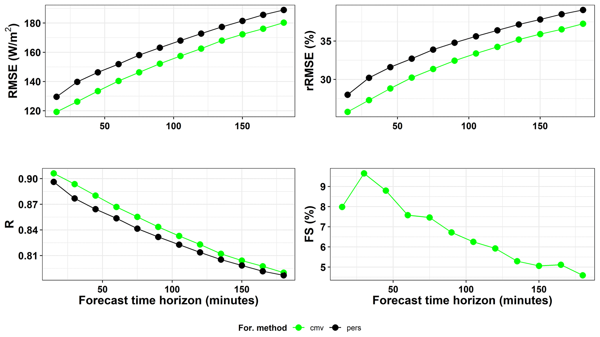
Figure 11Performance statistics for forecasted global horizontal irradiance (GHI) by the CMV model (green points) and by the persistence method (black points) for every 15 min time step up to 3 h ahead.
Table 4Performance statistics for CMV-forecasted global horizontal irradiance (GHI) for the 60, 120, and 180 min time steps.
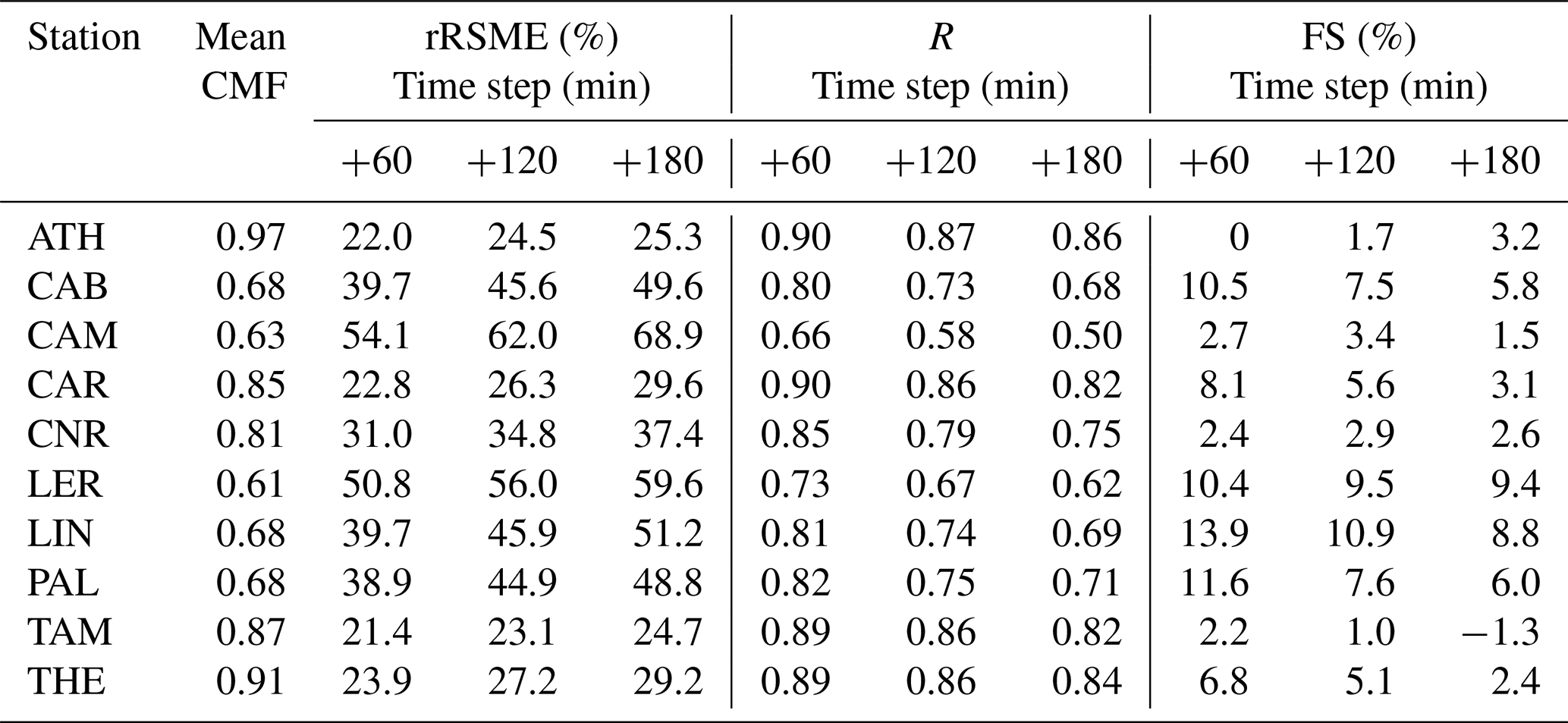
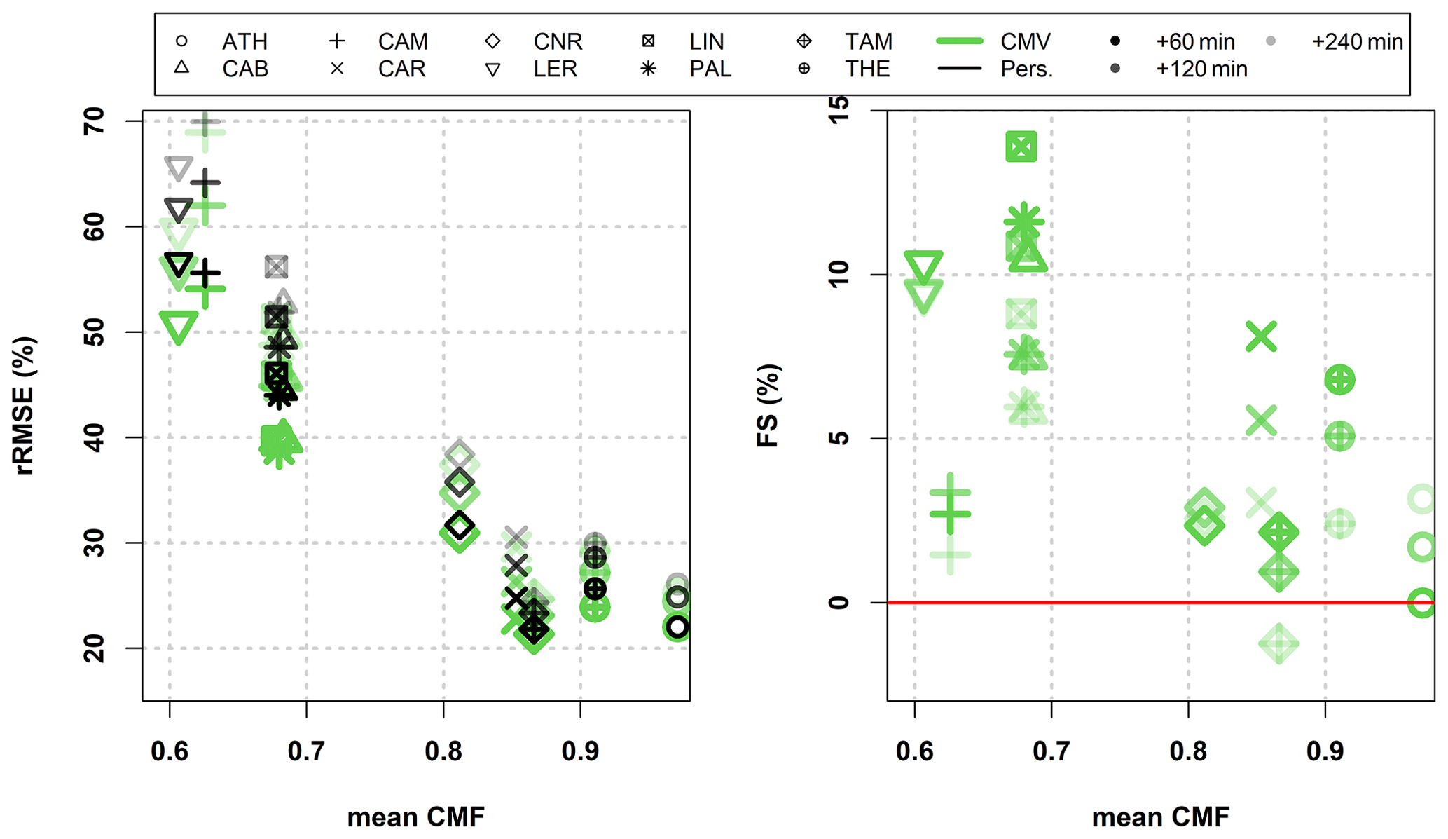
Figure 12Relative root mean square error (rRMSE%) and forecasting skill expressed as a percentage (FS%) for the CMV model (green symbols) and the persistence method (black symbols) when they were used to forecast global horizontal irradiance (GHI) versus the average cloudiness of stations (mean CMF) for the time steps (in order of increasingly transparent symbols) +60, +120, and +240 min.
An interesting grouping of stations was obtained by comparing the main statistics (rRMSE and FS) for both forecasting methods with the mean CMF (representing its mean cloudiness) for each station (Fig. 12). Three time steps were selected: +60, +120, and +180 min (in order of increasingly transparent symbols in the plot). Two groups of stations are evident: those with high mean cloudiness (LER, CAM, PAL, LIN, and CAB), which show worse rRMSEs than those with lower cloudiness (ATH, THE, TAM, CAR and CNR), independently of the method used. Again, the CMV model (green symbols) outperforms the persistence method (black symbols) for all stations for these time steps (except +240 min for TAM). The interesting finding is that the FS (%) of the CMV method increases with decreasing CMF; in other words, the forecasting skill of the CMV model is higher compared to persistence for stations with higher cloudiness, demonstrating the applicability of the CMV method of forecasting GHI under cloudy conditions.
3.2.2 Performance for different cloudy conditions
To demonstrate the value of the CMV model compared to the persistence method, which assumes the same cloudy conditions for all future time steps, we compared their performance under different cloudy conditions and transitions in cloudiness. Figure 13 presents the RMSEs for both models (green points for CMV and black points for persistence) and the CMV model FS% as a function of CMF for three time steps (+60, +120, and +180 min). Persistence performs better than the CMV model under clear-sky conditions, namely when CMF = 1, for all time steps (as expected, as there is no change in cloudiness). This is also true for CMF bin 0.9 for the +180 min time step only and for CMF bin > 1 (a bin which mainly contains clear-sky cases) for all time steps. For cloudy conditions, namely when CMF < 0.9, the CMV model outperforms persistence for all time steps (apart from +180 min when considering CMF bin 0.9). The cloudier the conditions (the smaller the CMF), the better the performance of the CMV model and the greater the CMV FS% (which is up to ∼ 20 % for the +60 min time step). The FS of CMV model decreases slightly with forecasting horizon; however, for the maximum forecasting horizon (+180 min), it remains quite high (∼ +10 %) for CMF bins < 0.7.
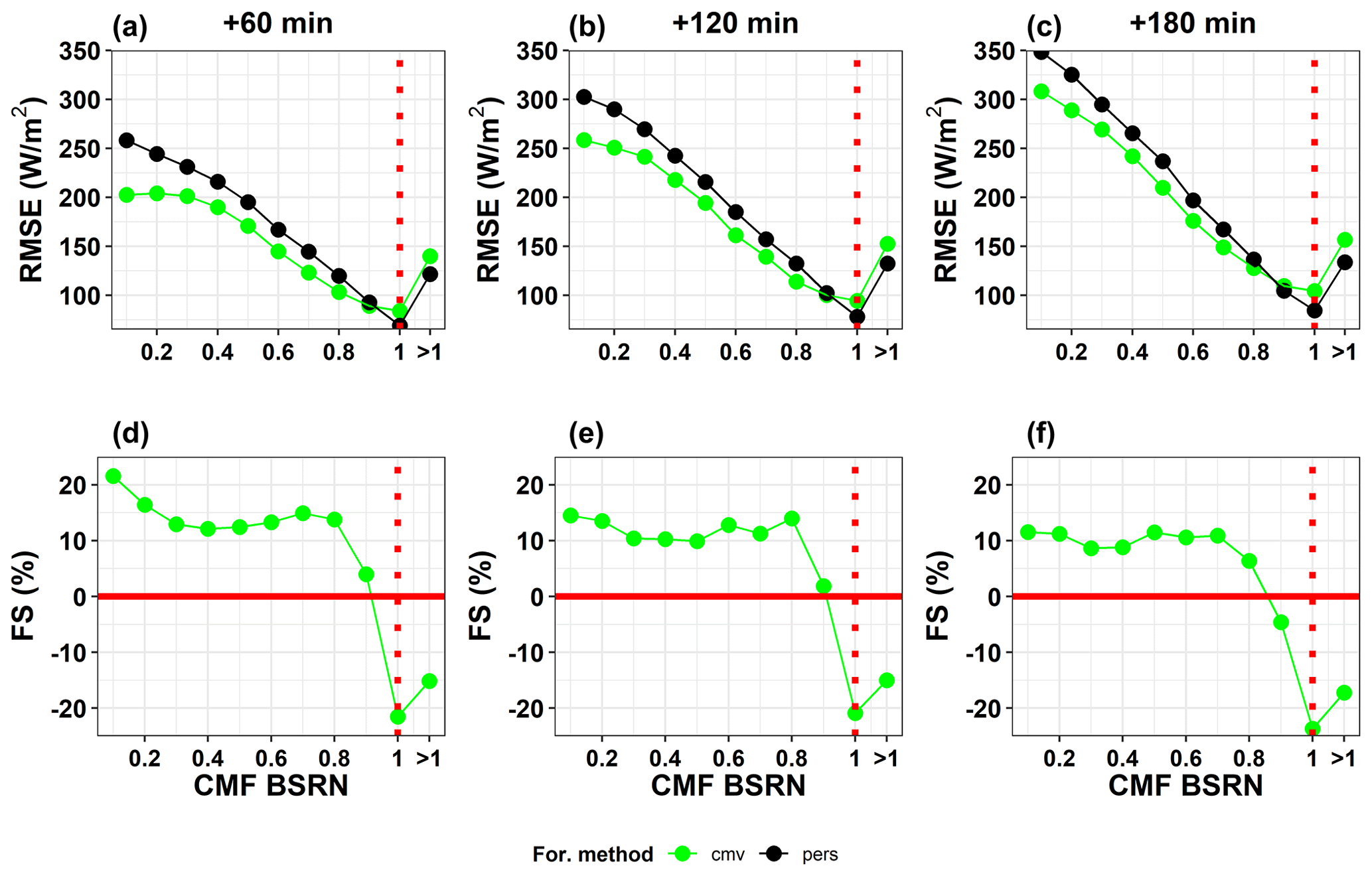
Figure 13(a–c) Root mean square error (RMSE) of the global horizontal irradiance (GHI) for all stations forecasted with the CMV model (green symbols) and with the persistence method (black symbols) versus the cloud modification factor (CMF) derived from GHI measurements for three time steps (+60, +120, and +180 min). (d–f) The CMV model's forecasting skill plotted against CMF class for the same time steps as used for panels (a)–(c), respectively.
To demonstrate the better performance of the CMV method compared to the persistence method for all time steps under cloudy conditions, we calculated CMV FS% for partially cloudy conditions (0.4 < CMF < 0.9) and overcast conditions (CMF ≤ 0.4), and the results are presented in Fig. 14. We can see again that the FS of the CMV model decreases with time; however, the minimum value is ∼ 10 % for both categories. The maximum FS occurs at the +15 min time step for both categories (at ∼ 16 % and ∼ 22 % for 0.4 < CMF < 0.9 (cross symbols) and CMF ≤ 0.4 (triangle symbols), respectively).
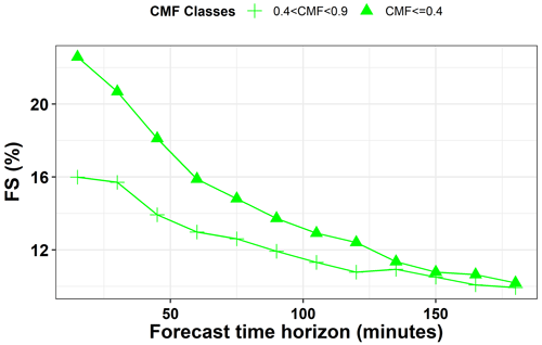
Figure 14Forecasting skill (FS, expressed as a percentage) of the CMV model against the persistence method for all stations as a function of time horizon for two different cloudiness conditions: 0.4 < CMF < 0.9 (crosses) and CMF ≤ 0.4 (triangles).
The performance of the CMV model against the persistence method was also assessed under changing cloudiness, evaluated as the CMF change based on ground-based measurements. The CMF changes were calculated for a time interval of 60 min (as ΔCMF = CMFt+60 − CMFt), and the results for the CMV model FS (%) are presented for the +60 min time step as a function of CMF change in Fig. 15. The high negative value of FS for the zero CMF change bin indicates that the persistence method is better for that bin, which was anticipated since there is zero or almost zero change in CMF, which is practically the definition of the persistence method. Persistence is still better than CMV for CMF changes from cloudy to clearer conditions up to the +0.3 CMF change bin, but the FS is less negative than for the zero bin. For CMF changes from cloudy to clearer conditions with higher magnitudes (bins > 0.4), CMV is better than persistence, with an FS value of 15 % for the +0.6 CMF change bin. Consistent results were found for the opposite situation, namely changes from clearer to cloudy conditions, with the CMV model always giving better FS values (of up to ∼ 20 %) than persistence.
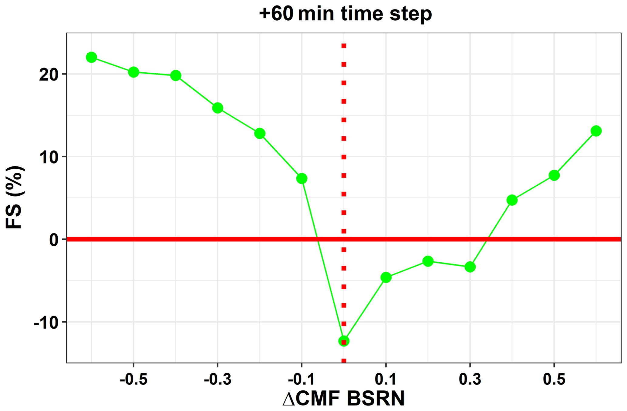
Figure 15Forecasting skill (FS, expressed as a percentage) of the CMV model against the persistence method for all stations as a function of CMF change within a 60 min time interval (from time 0 to the +60 min time step).
Our analysis for different cloudiness conditions highlights the limited ability of the persistence method compared to the CMV-based NextSENSE2 to accurately forecast GHI under cloudy conditions (CMF values < 0.9) and to follow transitions in cloudiness (especially those from clearer to cloudy conditions).
A direct comparison of the results of the present study for the NextSENSE2 short-term forecasting model with other studies is not straightforward, as the study period, the geographical area, and the validation methods used are different. Kallio-Myers et al. (2020) validated their Solis–Heliosat satellite-based GHI forecast modeled over southern Finland, and they found that the rRMSE reached 50 % at the 4 h time step. Urbich et al. (2019) validated SESORA short-term forecasts of solar surface irradiance over Germany and parts of Europe for 17 different cases with different weather patterns for the period August to October 2017, with all forecasts initiated at 09:15 UTC. For validation against the SARAH-2 data by CM SAF, they reported an RMSE of 59 W m−2 after 15 min and a maximum RMSE of 142 W m−2, reached after 165 min.
One of the limitations and sources of error for NextSENSE2 is related to the satellite-based optical flow method used for short-term forecasting: this method cannot reproduce cloud formation or dissipation. One example of this is convective clouds that form very fast, violating the optical flow criterion, i.e., that there should be constant intensity of the pixels between two consecutive images (e.g., Urbich et al., 2018, 2019). Urbich et al. (2018) applied the common approach of separation into subscales for the optimization process, which ultimately did not improve the forecast and increased the complexity of the implementation. As has already been discussed in the “Introduction”, satellite-based short-term forecasting is the best choice for a time horizon of up to 6 h ahead, since it is available in real time and at high spatial resolution. However, merging it with NWP models is a solution for increasing the time horizon and the quality of forecasts (Lorenz et al., 2012; Wolff et al., 2016), as it compensates for the effect of changes in intensities (during convection or cloud dissipation) that cannot be captured by CMV models (Müller and Pfeifroth, 2022). A comparison of a short-term forecasting model of surface solar radiation (the SESORA model) with different NWP models (apart with the persistence model) has been presented by Urbich et al. (2019), and they found that the intersection point where the NWP model delivers better results depends on the model and is beyond 3–4 h, which is also in line with the findings of other studies (e.g., Lorenz et al., 2012; Wolff et al., 2016). The merge of our short-term forecasting model with an NWP model is out of the scope of the present study. The elaborative benchmark analysis of the NextSENSE2 system against the persistence approach has demonstrated its applicability as an operational tool for a time horizon of up to 3 h ahead.
Our motivation is the continuous improvement of EO-based estimates and the accuracy of short-term forecasts of available solar resources to support solar energy exploitation systems at a regional scale (in Europe and the MENA region). In this study, we improved the SENSE nowcasting and NextSENSE short-term forecasting operational systems, and we analyzed cloud-related uncertainties in detail, using ground-based measurements to discriminate between different sun visibility conditions.
In terms of the aerosol-related inputs, a slight overestimation of CAMS AOD against AERONET retrievals (< 10 %) was found, which resulted in a SENSE2 clear-sky GHI underestimation of less than 1 %, highlighting the applicability of CAMS forecasts as EO inputs for operational solar resource nowcasting. In terms of modeled all-skies GHI, it was found that SENSE2 mostly overestimates GHI, with an MBE of 23.8 W m−2 (4.9 %) for instantaneous comparisons, which was attributed to the uncertainties related to satellite cloud retrievals (overestimation of CMFmsg by ∼ 0.02) and also to the spatial representativeness of satellite-based retrievals compared to ground-based measurements. We demonstrated that the most difficult situations to model are those with high spatial variability of solar radiation within the satellite pixel due to clouds (e.g., small broken clouds and the sun is obscured over the ground station, which is information that cannot be derived from satellite data). Based on our cloud-related analysis using ground-based data, a correction for the modeled GHI was used, resulting in an overall improvement in the SENSE2-modeled GHI such that 61 % of the cases were within ±50 W m−2 (±10 %) of the measured GHI and the final MBE of SENSE2 was 11.3 W m−2 (2.3 %). Our main analysis was based on the 15 min timescale; however, depending on the application, hourly, daily, or monthly data could be used. The daily and monthly SENSE2 GHI showed much better statistics (MBEs of 3.3 and 2.7 W m−2, respectively). The validation results for SENSE2 demonstrate highly accurate nowcasted values of GHI which are in line with similar models. The recorded positive bias could be reduced by applying improvements in the NWC SAF cloud retrieval input to SENSE2 regarding partially cloudy pixels. NextSENSE2 was also improved due to the SENSE2 improvements. We also showed that, compared to the persistence method, the model works much better (as expected) at locations with increased cloudiness and frequent cloudiness changes.
The data and methods involved in the estimation and prediction of the GHI in this study also revealed their limitations. As mentioned, the pixel-based approach for the model inputs (satellite and models) could not always reflect the reality above a (point) ground-based station. However, the model inputs are the state of the art for EO data and are readily available at a regional or global scale and at high spatial and temporal resolution; hence, the GHI product is representative of an area (∼ 5 km × 5 km in this model), which is useful for photovoltaic parks covering a wide area. In general, performance evaluations of such EO-based GHI models with ground-based measurements must account for these spatial representativity issues when performing comparisons. The optical flow algorithm for calculating CMVs is also based on assumptions like 2D clouds and brightness constancy. However, it is a method based on cloud inputs from satellite data in real time, and the applicability of such methods compared with the persistence approach was demonstrated here.
Since satellite cloud information is the only real-time input, a new straightforward configuration for estimating GHI was applied (SENSE2). The advantage of calculating clear-sky GHI from the previous day is what increases the accuracy of this product, since it is based on a detailed LUT of ∼ 16 million combinations of seven different inputs; apart from AOD, these include additional aerosol optical properties and atmosphere/surface state inputs. Thus, the uncertainties in the estimated clear-sky GHI practically only result from uncertainties in the model inputs. The new scheme for calculating the all-skies GHI by multiplying the clear-sky GHI by CMFmsg (derived in real time by a multi-parametric function of MSG COT and SZA) was improved by applying a suitable CMFmsg correction. The correction was successful and improved the model performance, especially for areas with high cloudiness. Additionally, the new configuration of SENSE2 is more flexible and it is easy to adapt so that it can provide more products (like DNI, the UV index, or PAR). Finally, running the model in a retrospective way using reanalysis data or in situ observational data for certain locations is one of the prospects for the new model.
According to the results, high-resolution (every 15 min at ∼ 5 km × 5 km) and quite accurate real-time GHI estimates and forecasts are produced from the upgraded SENSE2 and NextSENSE2 operational systems, respectively, which can contribute to solar energy systems management and planning.
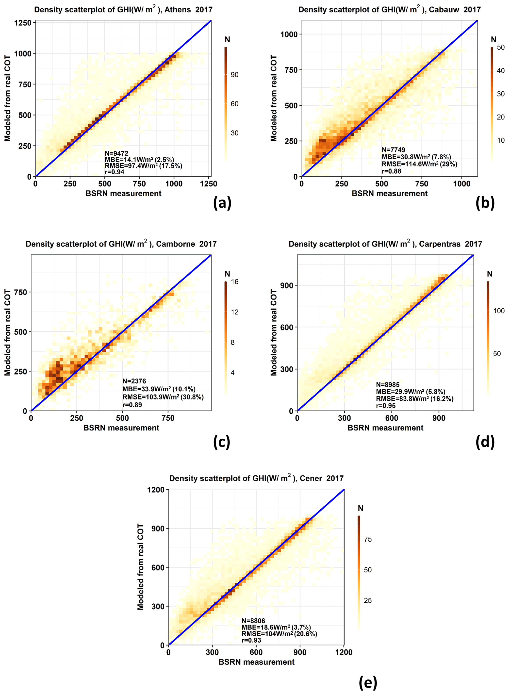
Figure A1Comparison of the modeled versus measured global horizontal irradiance (GHI) for (a) Athens, (b) Cabauw, (c) Camborne, (d) Carpentras, and (e) Cener for 2017.
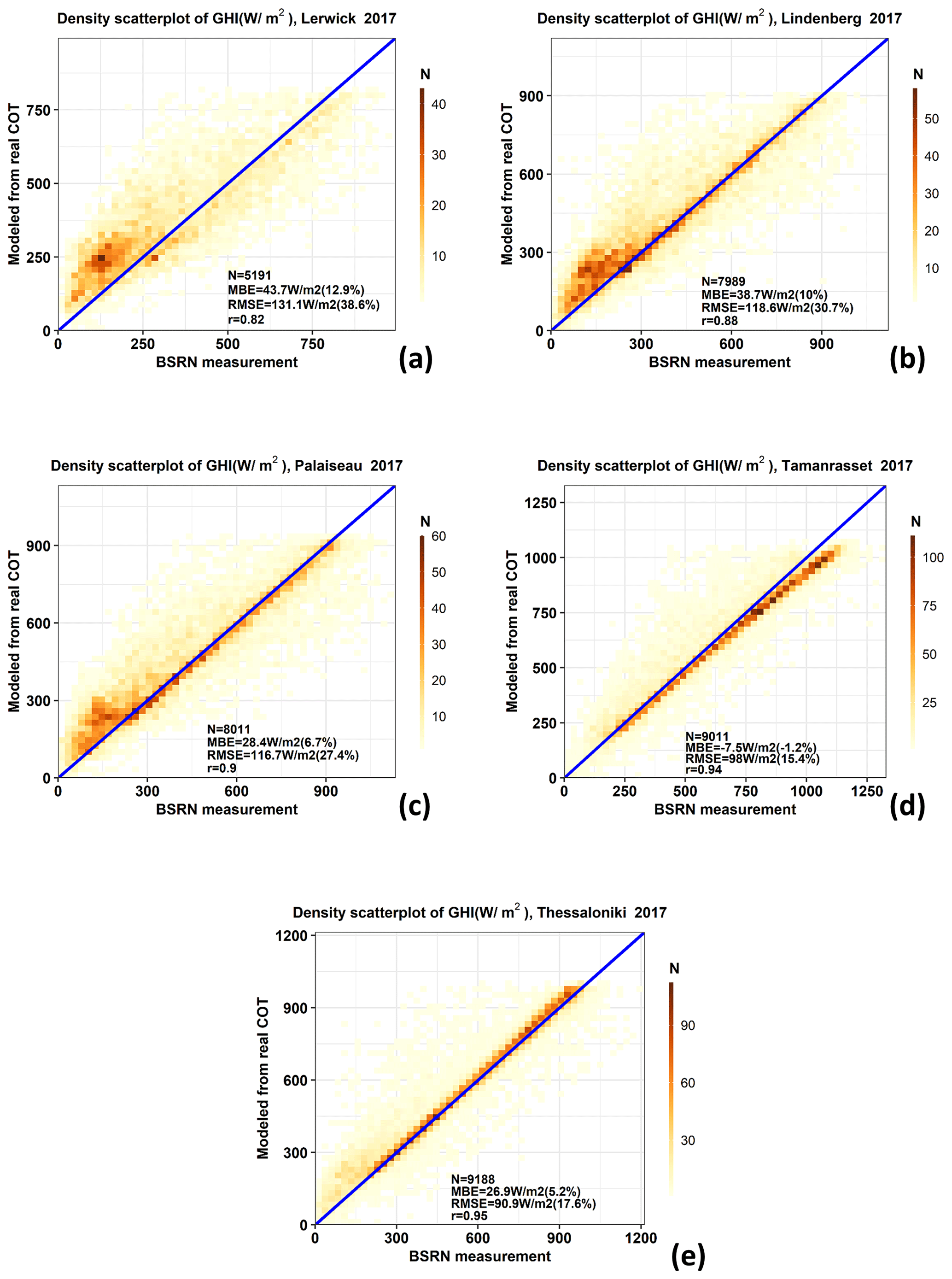
Figure A2Comparison of the modeled versus measured global horizontal irradiance (GHI) for (a) Lerwick, (b) Lindenberg, (c) Palaiseau, (d) Tamanrasset, and (e) Thessaloniki for 2017.
To see if the CMF difference (modeled against measured values) changed with SZA, the MBE of CMF was calculated for 10° bins of SZA. The measured CMF was considered to be the one derived from GHI measurements (Eq. 7) and the modeled one was derived using Eq. (2). The results are presented in Fig. A1 for all cases and under different cloudiness conditions, along with the relative values of CMF MBE expressed as percentages. We can again see that most of the overestimation of CMF values by MSG COT occurs for cloudy conditions (CMF < 0.9). Specifically, for partially cloudy conditions (0.4 < CMF < 0.9), the MBE reaches values of up to ∼ 0.20, and for overcast skies (CMF ≤ 0.4), there are SZA bins (0°) for which the MBE reaches values of up to 0.25. However, the MBE hardly changes with SZA for those two categories.
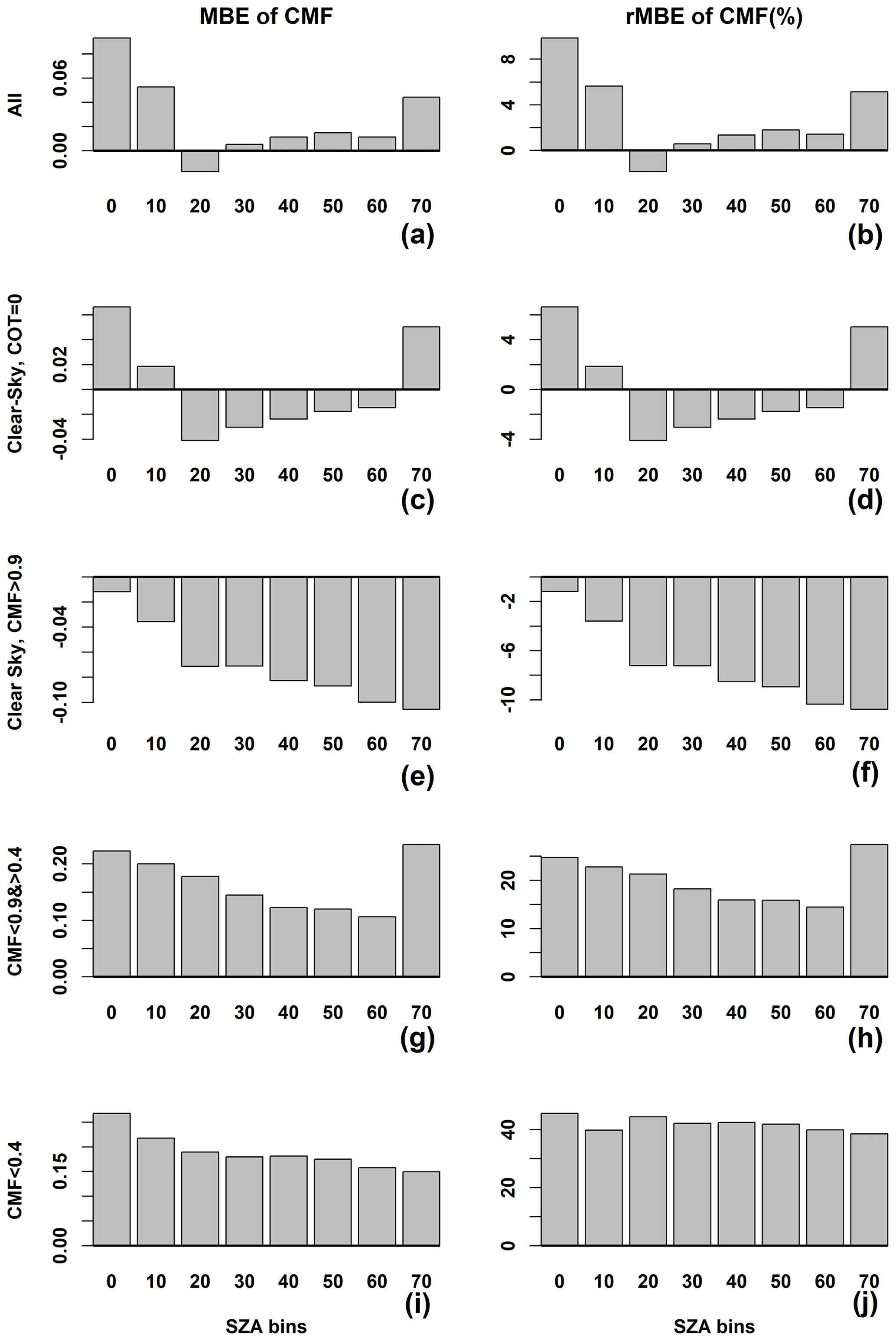
Figure B1Cloud modification factor (CMF) mean bias error (MBE – left column) and relative MBE (% – right column) as functions of solar zenith angle (SZA) for all cases and different cloudiness conditions.
The code used in this paper is available upon request from the authors.
The OMI TOC data are available from the NASA Goddard Space Flight Center, Goddard Earth Sciences Data and Information Services Center at https://doi.org/10.5067/Aura/OMI/DATA3001 (Bhartia, 2012). The CAMS global forecasts of aerosols are available from Atmosphere Data Store (ADS) at https://ads.atmosphere.copernicus.eu/cdsapp#\!/dataset/cams-global-atmospheric-composition-forecasts?tab=form, European Commission, 2024) or the ECMWF FTP server at https://www.ecmwf.int/en/forecasts/accessing-forecasts (ECMWF, 2024). The rest of data used in this paper are available upon request from the authors.
Idea and initialization: KP and SK; model parameterization: IF, KP, IPR; resources: AFB, BEP, IPR, CK; data provision and curation: AFB and BEP; cloud function approach: NP and AK; overview and revision: CK, MH, SK; first draft writing, visualization, analysis, and interpretation: KP; writing, review, and editing: all authors. All authors gave final approval for publication.
The contact author has declared that none of the authors has any competing interests.
This study contains modified Copernicus Atmosphere Monitoring Service information [2023], and neither the European Commission nor ECMWF is responsible for any use that may be made of the Copernicus information or data it contains.
Publisher’s note: Copernicus Publications remains neutral with regard to jurisdictional claims made in the text, published maps, institutional affiliations, or any other geographical representation in this paper. While Copernicus Publications makes every effort to include appropriate place names, the final responsibility lies with the authors.
We would like to thank the eight site instrument operators and technical staff of the BSRN network stations who made the ground-based measurements feasible. We acknowledge the principal investigators and co-investigators and their staff for establishing and maintaining the 10 AERONET sites used in this study. We acknowledge the EUMETSAT NWC SAF services as well as the OMI team for providing all the necessary data used in this study. We acknowledge the free use of the GOME-2 surface LER database provided through the AC SAF of EUMETSAT. The GOME-2 surface LER database was created by the Royal Netherlands Meteorological Institute (KNMI). This work was supported by computational time granted by the National Infrastructures for Research and Technology S.A. (GRNET) at the National HPC facility – ARIS – under project ID pa210301-SO-LISIS. Charalampos Kontoes, Stelios Kazadzis, Ilias Fountoulakis, and Kyriakoula Papachristopoulou would like to acknowledge the European Commission project “EXCELSIOR”: ERATOSTHENES: Excellence Research Centre for Earth Surveillance and Space-Based Monitoring of the Environment (grant no. 857510) and the European Commission project EuroGEO e-shape (GA no. 820852). Andreas Kazantzidis would like to acknowledge the co-financing by the European Union and Greek national funds through the Operational Program Competitiveness, Entrepreneurship and Innovation under the call RESEARCH–CREATE–INNOVATE (project code: T1EDK-00681). Stelios Kazadzis, Ilias Fountoulakis, and Kyriakoula Papachristopoulou would like to acknowledge the COST Action HARMONIA, CA21119, supported by COST (European Cooperation in Science and Technology).
This research has been supported by “EXCELSIOR”: ERATOSTHENES: Excellence Research Centre for Earth Surveillance and Space-Based Monitoring of the Environment (grant no. 857510).
This paper was edited by Oleg Dubovik and reviewed by three anonymous referees.
Anderson, G. P., Clough, S. A., Kneizys, F. X., Chetwynd, J. H., and Shettle, E. P.: AFGL atmospheric constituent profiles (0.120 km), Air Force Geophysics Lab Hanscom AFB MA, 1986
Arvizu, D., Balaya, P., Cabeza, L., Hollands, T., Jäger-Waldau, A., Kondo, M., Konseibo, C., Meleshko, V., Stein, W., Tamaura, Y., Xu, H., and Zilles, R.: Direct Solar Energy. In IPCC Special Report on Renewable Energy Sources and Climate Change Mitigation, edited by: Edenhofer, O., Pichs-Madruga, R., Sokona, Y., Seyboth, K., Matschoss, P., Kadner, S., Zwickel, T., Eickemeier, P., Hansen, G.,Schlömer, S., and von Stechow, C., Cambridge University Press, Cambridge, United Kingdom and New York, NY, USA, 2011.
Bais, A. F., Drosoglou, T., Meleti, C., Tourpali, K., and Kouremeti, N.: Changes in surface shortwave solar irradiance from 1993 to 2011 at Thessaloniki (Greece), Int. J. Climatol., 33, 2871–2876, https://doi.org/10.1002/joc.3636, 2013.
Basart, S., Langerock, B., Arola, A., Benedictow, A., Bennouna, Y., Bouarar, I., Cuevas, E., Errera, Q., Eskes, H. J., Griesfeller, J., Kapsomenakis, J., Mortier, A., Pison, I., Pitkänen, M., Ramonet, M., Richter, A., Schoenhardt, A., Schulz, M., Tarniewicz, J., Thouret, V., Tsikerdekis, A., Warneke, T., and Zerefos, C.: Validation report of the CAMS near-real-time global atmospheric composition service: June–August 2022, Copernicus Atmosphere Monitoring Service (CAMS) report, https://doi.org/10.24380/tstx-k064, 2023.
Bhartia, P. K.: OMI/Aura TOMS-Like Ozone, Aerosol Index, Cloud Radiance Fraction L3 1 day 1 degree x 1 degree V3, NASA Goddard Space Flight Center, Goddard Earth Sciences Data and Information Services Center (GES DISC) [data set], https://doi.org/10.5067/Aura/OMI/DATA3001, 2012.
Buras, R., Dowling, T., and Emde, C.: New secondary-scattering correction in DISORT with increased efficiency for forward scattering, J. Quant. Spectrosc. Radiat. Transf., 112, 2028–2034, https://doi.org/10.1016/j.jqsrt.2011.03.019, 2011.
Cano, D., Monget, J. M., Albuisson, M., Guillard, H., Regas, N., and Wald, L.: A Method For The Determination Of The Global Solar Radiation From Meteorological Satellite Data, 31–39, https://doi.org/10.1016/0038-092X(86)90104-0, 1986.
Carpentieri, A., Folini, D., Wild, M., Vuilleumier, L., and Meyer, A.: Satellite-derived solar radiation for intra-hour and intra-day applications: Biases and uncertainties by season and altitude, Sol. Energy, 255, 274–284, https://doi.org/10.1016/j.solener.2023.03.027, 2023.
Derrien, M. and Le Gléau, H.: MSG/SEVIRI cloud mask and type from SAFNWC, Int. J. Remote Sens., 26, 4707–4732, https://doi.org/10.1080/01431160500166128, 2005.
Driemel, A., Augustine, J., Behrens, K., Colle, S., Cox, C., Cuevas-Agulló, E., Denn, F. M., Duprat, T., Fukuda, M., Grobe, H., Haeffelin, M., Hodges, G., Hyett, N., Ijima, O., Kallis, A., Knap, W., Kustov, V., Long, C. N., Longenecker, D., Lupi, A., Maturilli, M., Mimouni, M., Ntsangwane, L., Ogihara, H., Olano, X., Olefs, M., Omori, M., Passamani, L., Pereira, E. B., Schmithüsen, H., Schumacher, S., Sieger, R., Tamlyn, J., Vogt, R., Vuilleumier, L., Xia, X., Ohmura, A., and König-Langlo, G.: Baseline Surface Radiation Network (BSRN): structure and data description (1992–2017), Earth Syst. Sci. Data, 10, 1491–1501, https://doi.org/10.5194/essd-10-1491-2018, 2018.
ECMWF: Access to forecasts, https://www.ecmwf.int/en/forecasts/accessing-forecasts (last access: 6 March 2024), 2024.
Edenhofer, O., Pichs-Madruga, R., Sokona, Y., Seyboth, K., Matschoss, P., Kadner, S., Zwickel, T., Eickemeier, P., Hansen, G., and Schlömer, S.: IPCC special report on renewable energy sources and climate change mitigation, Prepared By Working Group III of the Intergovernmental Panel on Climate Change, Cambridge University Press, Cambridge, UK, ISBN 978-1-107-02340-6, 2011.
Emde, C., Buras-Schnell, R., Kylling, A., Mayer, B., Gasteiger, J., Hamann, U., Kylling, J., Richter, B., Pause, C., Dowling, T., and Bugliaro, L.: The libRadtran software package for radiative transfer calculations (version 2.0.1), Geosci. Model Dev., 9, 1647–1672, https://doi.org/10.5194/gmd-9-1647-2016, 2016.
Eskes, H. J., Basart, S., Benedictow, A., Bennouna, Y., Blechschmidt, A.-M., Chabrillat, S., Cuevas, E., Errera, Q., Flentje, H., Hansen, K. M., Kapsomenakis, J., Langerock, B., Ramonet, M., Richter, A., Schulz, M., Sudarchikova, N., Wagner, A., Warneke, T., and Zerefos, C.: Observation characterisation and validation methods document, Copernicus Atmosphere Monitoring Service (CAMS) report, https://doi.org/10.24380/3b4exb93, 2021.
European Commission: CAMS global atmospheric composition forecasts, European Commission [data set], https://ads.atmosphere.copernicus.eu/cdsapp#!/dataset/cams-global-atmospheric-composition-forecasts?tab=form (last access: 19 March 2024), 2024.
Farnebäck, G.: Two-Frame Motion Estimation Based on Polynomial Expansion, in: Lecture Notes in Computer Science, 2749, 363–370, https://doi.org/10.1007/3-540-45103-X_50, edited by: Bigun J. and Gustavvson, T., Springer-Verlag Berlin Heidelberg 2003, 2003.
Fountoulakis, I., Kosmopoulos, P., Papachristopoulou, K., Raptis, I. P., Mamouri, R. E., Nisantzi, A., Gkikas, A., Witthuhn, J., Bley, S., Moustaka, A., Buehl, J., Seifert, P., Hadjimitsis, D. G., Kontoes, C., and Kazadzis, S.: Effects of aerosols and clouds on the levels of surface solar radiation and solar energy in cyprus, Remote Sens.-Basel, 13, 1–26, https://doi.org/10.3390/rs13122319, 2021.
Garniwa, P. M. P., Rajagukguk, R. A., Kamil, R., and Lee, H. J.: Intraday forecast of global horizontal irradiance using optical flow method and long short-term memory model, Sol. Energy, 252, 234–251, https://doi.org/10.1016/j.solener.2023.01.037, 2023.
Gasteiger, J., Emde, C., Mayer, B., Buras, R., Buehler, S. A., and Lemke, O.: Representative wavelengths absorption parameterization applied to satellite channels and spectral bands, J. Quant. Spectrosc. Radiat. Transf., 148, 99–115, https://doi.org/10.1016/j.jqsrt.2014.06.024, 2014.
Giles, D. M., Sinyuk, A., Sorokin, M. G., Schafer, J. S., Smirnov, A., Slutsker, I., Eck, T. F., Holben, B. N., Lewis, J. R., Campbell, J. R., Welton, E. J., Korkin, S. V., and Lyapustin, A. I.: Advancements in the Aerosol Robotic Network (AERONET) Version 3 database – automated near-real-time quality control algorithm with improved cloud screening for Sun photometer aerosol optical depth (AOD) measurements, Atmos. Meas. Tech., 12, 169–209, https://doi.org/10.5194/amt-12-169-2019, 2019.
Gschwind, B., Wald, L., Blanc, P., Lefèvre, M., Schroedter-Homscheidt, M., and Arola, A.: Improving the McClear model estimating the downwelling solar radiation at ground level in cloud-free conditions – McClear-v3, Meteorol. Z., 28, 147–163, https://doi.org/10.1127/metz/2019/0946, 2019.
Habte, A., Sengupta, M., and Lopez, A.: Evaluation of the national solar radiation database (NSRDB): 1998–2015, National Renewable Energy Lab. (NREL), Golden, CO, United States, https://doi.org/10.2172/1351859, 2017.
Hammer, A., Heinemann, D., Lorenz, E., and Lückehe, B.: Short-term forecasting of solar radiation: A statistical approach using satellite data, Sol. Energy, 67, 139–150, https://doi.org/10.1016/s0038-092x(00)00038-4, 1999.
Hammer, A., Heinemann, D., Hoyer, C., Kuhlemann, R., Lorenz, E., Müller, R., and Beyer, H. G.: Solar energy assessment using remote sensing technologies, Remote Sens. Environ., 86, 423–432, https://doi.org/10.1016/S0034-4257(03)00083-X, 2003.
Holben, B. N., Eck, T. F., Slutsker, I., Tanré, D., Buis, J. P., Setzer, A., Vermote, E., Reagan, J. A., Kaufman, Y. J., Nakajima, T., Lavenu, F., Jankowiak, I., and Smirnov, A.: AERONET – A federated instrument network and data archive for aerosol characterization, Remote Sens. Environ., 66, 1–16, https://doi.org/10.1016/S0034-4257(98)00031-5, 1998.
Hu, Y. X. and Stamnes, K.: An accurate parameterization of the radiative properties of water clouds suitable for use in climate models, J. Climate, 6, 728–742, 1993.
IEA: Renewables 2022, IEA, Paris, https://www.iea.org/reports/renewables-2022 (last access: 6 March 2024), Licence: CC BY 4.0, 2022.
Ineichen, P. and Perez, R.: A New Airmass Independent Formulation For The Linke Turbidity Coefficient, 151–157, https://doi.org/10.1016/S0038-092X(02)00045-2, 2002.
Inness, A., Ades, M., Agustí-Panareda, A., Barré, J., Benedictow, A., Blechschmidt, A.-M., Dominguez, J. J., Engelen, R., Eskes, H., Flemming, J., Huijnen, V., Jones, L., Kipling, Z., Massart, S., Parrington, M., Peuch, V.-H., Razinger, M., Remy, S., Schulz, M., and Suttie, M.: The CAMS reanalysis of atmospheric composition, Atmos. Chem. Phys., 19, 3515–3556, https://doi.org/10.5194/acp-19-3515-2019, 2019.
IPCC: Summary for Policymakers, edited by: Pörtner, H.-O., Roberts, D. C., Poloczanska, E. S., Mintenbeck, K., Tignor, M., Alegría, A., Craig, M., Langsdorf, S., Löschke, S., Möller, V.,and Okem, A., in: Climate Change 2022: Impacts, Adaptation and Vulnerability, Contribution of Working Group II to the Sixth Assessment Report of the Intergovernmental Panel on Climate Change, edited by: Pörtner, H.-O., Roberts, D. C., Tignor, M., Poloczanska, E. S., Mintenbeck, K., Alegría, A., Craig, M., Langsdorf, S., Löschke, S., Möller, V., Okem, A., and Rama, B., Cambridge University Press, Cambridge, UK and New York, NY, USA, 3–33, https://doi.org/10.1017/9781009325844.001, 2022.
Kallio-Myers, V., Riihelä, A., Lahtinen, P., and Lindfors, A.: Global horizontal irradiance forecast for Finland based on geostationary weather satellite data, Sol. Energy, 198, 68–80, https://doi.org/10.1016/j.solener.2020.01.008, 2020.
Kazadzis, S., Bais, A., Balis, D., Kouremeti, N., Zempila, M., Arola, A., Giannakaki, E., Amiridis, V., and Kazantzidis, A.: Spatial and temporal UV irradiance and aerosol variability within the area of an OMI satellite pixel, Atmos. Chem. Phys., 9, 4593–4601, https://doi.org/10.5194/acp-9-4593-2009, 2009.
Kazadzis, S., Founda, D., Psiloglou, B. E., Kambezidis, H., Mihalopoulos, N., Sanchez-Lorenzo, A., Meleti, C., Raptis, P. I., Pierros, F., and Nabat, P.: Long-term series and trends in surface solar radiation in Athens, Greece, Atmos. Chem. Phys., 18, 2395–2411, https://doi.org/10.5194/acp-18-2395-2018, 2018.
Kinne, S.: The MACv2 aerosol climatology, Tellus B, 71, 1–21, https://doi.org/10.1080/16000889.2019.1623639, 2019.
Kosmopoulos, P., Kouroutsidis, D., Papachristopoulou, K., Raptis, P. I., Masoom, A., Saint-Drenan, Y. M., Blanc, P., Kontoes, C., and Kazadzis, S.: Short-term forecasting of large-scale clouds impact on downwelling surface solar irradiation, Energies (Basel), 13, 6555, https://doi.org/10.3390/en13246555, 2020.
Kosmopoulos, P. G., Kazadzis, S., Taylor, M., Raptis, P. I., Keramitsoglou, I., Kiranoudis, C., and Bais, A. F.: Assessment of surface solar irradiance derived from real-time modelling techniques and verification with ground-based measurements, Atmos. Meas. Tech., 11, 907–924, https://doi.org/10.5194/amt-11-907-2018, 2018.
Kosmopoulos, P. G., Kazadzis, S., Schmalwieser, A. W., Raptis, P. I., Papachristopoulou, K., Fountoulakis, I., Masoom, A., Bais, A. F., Bilbao, J., Blumthaler, M., Kreuter, A., Siani, A. M., Eleftheratos, K., Topaloglou, C., Gröbner, J., Johnsen, B., Svendby, T. M., Vilaplana, J. M., Doppler, L., Webb, A. R., Khazova, M., De Backer, H., Heikkilä, A., Lakkala, K., Jaroslawski, J., Meleti, C., Diémoz, H., Hülsen, G., Klotz, B., Rimmer, J., and Kontoes, C.: Real-time UV index retrieval in Europe using Earth observation-based techniques: system description and quality assessment, Atmos. Meas. Tech., 14, 5657–5699, https://doi.org/10.5194/amt-14-5657-2021, 2021.
Kurucz, R. L.: Synthetic Infrared Spectra, Symposium – International Astronomical Union, 154, 523–531, https://doi.org/10.1017/S0074180900124805, 1994.
Lefèvre, M., Oumbe, A., Blanc, P., Espinar, B., Gschwind, B., Qu, Z., Wald, L., Schroedter-Homscheidt, M., Hoyer-Klick, C., Arola, A., Benedetti, A., Kaiser, J. W., and Morcrette, J.-J.: McClear: a new model estimating downwelling solar radiation at ground level in clear-sky conditions, Atmos. Meas. Tech., 6, 2403–2418, https://doi.org/10.5194/amt-6-2403-2013, 2013.
Long, C. N. and Dutton, E. G.: BSRN Global Network recommended QC tests, V2.x, https://epic.awi.de/id/eprint/30083/1/BSRN_recommended_QC_tests_V2.pdf (last access: 13 March 2024), 2010.
Lorenz, E., Hammer, A., and Heienmann, D.: Short term forecasting of solar radiation based on cloud motion vectors from satellite images, in: EUROSUN2004, ISES Europe Solar Congress, Freiburg/Brsg., 841–848, 2004
Lorenz, E., Kühnert, J., and Heinemann, D.: Short term forecasting of solar irradiance by combining satellite data and numerical weather predictions, in: Proceedings of the 27th European PV Solar Energy Conference (EU PVSEC), Frankfurt, Germany, WIP, Munchen, Germany, 44014405, ISBN 9783936338287, 3936338280, 2012.
Marie-Joseph, I., Linguet, L., Gobinddass, M. L., and Wald, L.: On the applicability of the Heliosat-2 method to assess surface solar irradiance in the Intertropical Convergence Zone, French Guiana, Int. J. Remote Sens., 34, 3012–3027, https://doi.org/10.1080/01431161.2012.756598, 2013.
Mayer, B.: Radiative transfer in the cloudy atmosphere, EPJ Web Conf., 1, 75–99, https://doi.org/10.1140/epjconf/e2009-00912-1, 2009.
Mayer, B. and Kylling, A.: Technical note: The libRadtran software package for radiative transfer calculations – description and examples of use, Atmos. Chem. Phys., 5, 1855–1877, https://doi.org/10.5194/acp-5-1855-2005, 2005.
Météo-France: Algorithm Theoretical Basis Document for the Cloud Product Processors of the NWC/GEO (GEO-CMA-v4.0, GEO-CT-v3.0, GEO-CTTH-v3.0, GEO-CMIC-v1.0), Technical Report NWC/CDOP2/GEO/MFL/SCI/ATBD/Cloud, Issue 1, Rev. 1, Météo-France, 2016.
Mueller, R., Behrendt, T., Hammer, A., and Kemper, A.: A new algorithm for the satellite-based retrieval of solar surface irradiance in spectral bands, Remote Sens.-Basel, 4, 622–647, https://doi.org/10.3390/rs4030622, 2012.
Mueller, R. W., Matsoukas, C., Gratzki, A., Behr, H. D., and Hollmann, R.: The CM-SAF operational scheme for the satellite based retrieval of solar surface irradiance – A LUT based eigenvector hybrid approach, Remote Sens. Environ., 113, 1012–1024, https://doi.org/10.1016/j.rse.2009.01.012, 2009.
Müller, R. and Pfeifroth, U.: Remote sensing of solar surface radiation – a reflection of concepts, applications and input data based on experience with the effective cloud albedo, Atmos. Meas. Tech., 15, 1537–1561, https://doi.org/10.5194/amt-15-1537-2022, 2022.
Müller, R., Pfeifroth, U., Träger-Chatterjee, C., Trentmann, J., and Cremer, R.: Digging the METEOSAT treasure-3 decades of solar surface radiation, Remote Sens.-Basel, 7, 8067–8101, https://doi.org/10.3390/rs70608067, 2015.
Oumbe, A.: Exploitation des nouvelles capacités d'observation de la terre pour évaluer le rayonnement solaire incident au sol (Assessment of solar surface radiation using new earth observation capabilities), PhD thesis, MINES ParisTech, HAL Id: pastel-00005759, 128 pp., 9 November 2009.
Oumbe, A., Qu, Z., Blanc, P., Lefèvre, M., Wald, L., and Cros, S.: Decoupling the effects of clear atmosphere and clouds to simplify calculations of the broadband solar irradiance at ground level, Geosci. Model Dev., 7, 1661–1669, https://doi.org/10.5194/gmd-7-1661-2014, 2014.
Papachristopoulou, K., Fountoulakis, I., Gkikas, A., Kosmopoulos, P. G., Nastos, P. T., Hatzaki, M., and Kazadzis, S.: 15-Year Analysis of Direct Effects of Total and Dust Aerosols in Solar Radiation/Energy over the Mediterranean Basin, Remote Sens.-Basel, 14, 1535, https://doi.org/10.3390/rs14071535, 2022.
Pelland, S., Remund, J., Kleissl, J., Oozeki, T., and De Brabandere, K.: Photovoltaic and solar forecasting: state of the art, IEA PVPS Task, 14, 1–36, 2013.
Pfeifroth, U. and Trentmann, J.: Algorithm Theoretical Baseline Document: Meteosat Solar Surface Radiation and effective Cloud Albedo Climate Data Records – Heliosat SARAH-3 The MAGICSOL method applied for the generation of SARAH-3, EUMETSAT Satellite Applications Facility on Climate Monitoring, Report SAF/CM/DWD/ATBD/SARAH, 3.5, https://www.cmsaf.eu/SharedDocs/Literatur/document/2023/saf_cm_dwd_atbd_sarah_3_5_pdf.pdf?__blob=publicationFile (last access: 6 March 2024), 2023.
Pfeifroth, U., Kothe, S., Drücke, J., Trentmann, J., Schröder, M., Selbach, N., and Hollmann, R.: Surface Radiation Data Set – Heliosat (SARAH) – Edition 3, Satellite Application Facility on Climate Monitoring [data set], https://doi.org/10.5676/EUM_SAF_CM/SARAH/V003, 2023a.
Pfeifroth U., Trentmann J., and Drücke J.: Validation Report Meteosat Solar Surface Radiation and Effective Cloud Albedo Climate Data Records SARAH-3, EUMETSAT Satellite Applications Facility on Climate Monitoring, https://doi.org/10.5676/EUM_SAF_CM/SARAH/V003, 2023b.
Qu, Z., Gschwind, B., Lefevre, M., and Wald, L.: Improving HelioClim-3 estimates of surface solar irradiance using the McClear clear-sky model and recent advances in atmosphere composition, Atmos. Meas. Tech., 7, 3927–3933, https://doi.org/10.5194/amt-7-3927-2014, 2014.
Qu, Z., Oumbe, A., Blanc, P., Espinar, B., Gesell, G., Gschwind, B., Klüser, L., Lefèvre, M., Saboret, L., Schroedter-Homscheidt, M., and Wald, L.: Fast radiative transfer parameterisation for assessing the surface solar irradiance: The Heliosat-4 method, Meteorol. Z., 26, 33–57, https://doi.org/10.1127/metz/2016/0781, 2017.
Rigollier, C., Lefèvre, M., and Wald, L.: The method Heliosat-2 for deriving shortwave solar radiation from satellite images, Sol. Energy, 77, 159–169, 2004.
Schenzinger, V., Kreuter, A., Klotz, B., Schwarzmann, M., and Gröbner, J.: On the production and validation of satellite based UV index maps, Atmos. Meas. Tech. Discuss. [preprint], https://doi.org/10.5194/amt-2023-188, 2023.
Schroedter-Homscheidt, M., Azam, F., Betcke, J., Hanrieder, N., Lefèvre, M., Saboret, L., and Saint-Drenan, Y. M.: Surface solar irradiation retrieval from MSG/SEVIRI based on APOLLO Next Generation and HELIOSAT-4 methods, Meteorol. Z., 31, 455–476, https://doi.org/10.1127/metz/2022/1132, 2022.
Sengupta, M., Xie, Y., Lopez, A., Habte, A., Maclaurin, G., and Shelby, J.: The National Solar Radiation Data Base (NSRDB), Renew. Sustain. Energy Rev., 89, 51–60, https://doi.org/10.1016/j.rser.2018.03.003, 2018.
Sengupta, M., Habte, A., Wilbert, S., Gueymard, C., and Remund, J.: Best practices handbook for the collection and use of solar resource data for solar energy applications, National Renewable Energy Lab. (NREL), Golden, CO, United States, https://doi.org/10.2172/1778700, 2021.
Shettle, E. P.: Models of aerosols, clouds and precipitation for atmospheric propagation studies, paper presented at Conference on Atmospheric Propagation in the UV, Visible, IR and MM-Region and Related System Aspects, NATO Adv. Group for Aerosp, Res. and Dev., Copenhagen, 1989.
Taylor, M., Kosmopoulos, P. G., Kazadzis, S., Keramitsoglou, I., and Kiranoudis, C. T.: Neural network radiative transfer solvers for the generation of high resolution solar irradiance spectra parameterized by cloud and aerosol parameters, J. Quant. Spectrosc. Radiat. Transf., 168, 176–192, https://doi.org/10.1016/j.jqsrt.2015.08.018, 2016.
Thomas, C., Wey, E., Blanc, P., Wald, L., and Lefèvre, M.: Validation of HelioClim-3 version 4, HelioClim-3 version 5 and MACC-RAD using 14 BSRN stations, Enrgy. Proced., 91, 1059–1069, https://doi.org/10.1016/j.egypro.2016.06.275, 2016.
Tijhuis, M., van Stratum, B. J. H., Veerman, M. A., and van Heerwaarden, C. C.: An Efficient Parameterization for Surface Shortwave 3D Radiative Effects in Large-Eddy Simulations of Shallow Cumulus Clouds, J. Adv. Model. Earth Syst., 15, 1, https://doi.org/10.1029/2022MS003262, 2023.
Tilstra, L. G., Tuinder, O. N. E., Wang, P., and Stammes, P.: Surface reflectivity climatologies from UV to NIR determined fromEarth observations by GOME-2 and SCIAMACHY, J. Geophys. Res., 122, 4084–4111, https://doi.org/10.1002/2016JD025940, 2017.
Tilstra, L. G., Tuinder, O. N. E., Wang, P., and Stammes, P.: Directionally dependent Lambertian-equivalent reflectivity (DLER) of the Earth's surface measured by the GOME-2 satellite instruments, Atmos. Meas. Tech., 14, 4219–4238, https://doi.org/10.5194/amt-14-4219-2021, 2021.
Urbich, I., Bendix, J., and Müller, R.: A novel approach for the short-term forecast of the effective cloud albedo, Remote Sens.-Basel, 10, 1–16, https://doi.org/10.3390/rs10060955, 2018.
Urbich, I., Bendix, J., and Müller, R.: The seamless solar radiation (SESORA) forecast for solar surface irradiance-method and validation, Remote Sens.-Basel, 11, 1–23, https://doi.org/10.3390/rs11212576, 2019.
Urraca, R., Gracia-Amillo, A. M., Koubli, E., Huld, T., Trentmann, J., Riihelä, A., Lindfors, A. V., Palmer, D., Gottschalg, R., and Antonanzas-Torres, F.: Extensive validation of CM SAF surface radiation products over Europe, Remote Sens. Environ., 199, 171–186, https://doi.org/10.1016/j.rse.2017.07.013, 2017.
Wolff, B., Kühnert, J., Lorenz, E., Kramer, O., and Heinemann, D.: Comparing support vector regression for PV power forecasting to a physical modeling approach using measurement, numerical weather prediction, and cloud motion data, Sol. Energy, 135, 197–208, https://doi.org/10.1016/j.solener.2016.05.051, 2016.
Yang, D.: SolarData package update v1.1: R functions for easy access of Baseline Surface Radiation Network (BSRN), Sol. Energy, 188, 970–975, https://doi.org/10.1016/j.solener.2019.05.068, 2019.
Yang, D., Wang, W., Gueymard, C. A., Hong, T., Kleissl, J., Huang, J., Perez, M. J., Perez, R., Bright, J. M., Xia, X., van der Meer, D., and Peters, I. M.: A review of solar forecasting, its dependence on atmospheric sciences and implications for grid integration: Towards carbon neutrality, Renew. Sustain. Energy Rev., 161, 112348, https://doi.org/10.1016/j.rser.2022.112348, 2022.
Yu, L., Zhang, M., Wang, L., Lu, Y., and Li, J.: Effects of aerosols and water vapour on spatial-temporal variations of the clear-sky surface solar radiation in China, Atmos. Res., 248, 105162, https://doi.org/10.1016/j.atmosres.2020.105162, 2021.