the Creative Commons Attribution 4.0 License.
the Creative Commons Attribution 4.0 License.
 | 17 Jul 2024
Unfiltering of the EarthCARE Broadband Radiometer (BBR) observations: the BM-RAD product
Almudena Velázquez Blázquez
Edward Baudrez
Nicolas Clerbaux
Carlos Domenech
The methodology to determine the unfiltered solar and thermal radiances from the measured EarthCARE Broadband Radiometer (BBR) shortwave (SW) and total-wave (TW) filtered radiances is presented. Within the EarthCARE ground processing, the correction for the effect of the BBR spectral responses, the unfiltering, is performed by the so-called BM-RAD processor which produces the level-2 BM-RAD product. The BM-RAD product refers to unfiltered broadband radiances that are derived from the BBR and the Multi-Spectral Imager (MSI) instruments on board the forthcoming EarthCARE satellite. The method is based on theoretical regressions between filtered and unfiltered radiances, as is done for the Clouds and the Earth's Radiant Energy System (CERES) and the Geostationary Earth Radiation Budget (GERB) instruments. The regressions are derived from a large geophysical database of spectral radiance curves simulated using radiative transfer models. Based on the radiative transfer computations, the unfiltering error, i.e., the error introduced by the small spectral variations of the BBR instrument response, is expected to remain well below 0.5 % in the shortwave (SW) and 0.1 % in the longwave (LW), at 1 standard deviation. These excellent performances are permitted by the very simple optics used in the BBR instrument: a telescope with a single paraboloid mirror. End-to-end verification of the unfiltering algorithm has been performed by running the BM-RAD processor on modelled level-1 BBR radiances obtained for three EarthCARE orbits simulated by an integrated forecasting and data assimilation system. The resulting unfiltered radiances are eventually compared to the solar and thermal radiances derived by radiative transfer simulations over the three EarthCARE orbits. In addition, this end-to-end verification has provided further evidence on the high accuracy of the unfiltered radiance process, with accuracies better than 0.5 % for SW and better than 0.1 % for LW.
- Article
(2660 KB) - Full-text XML
- BibTeX
- EndNote


The EarthCARE (Earth Cloud, Aerosol and Radiation Explorer) mission (Illingworth et al., 2015; Wehr et al., 2023) is a collaborative mission between the European Space Agency (ESA) and the Japan Aerospace Exploration Agency (JAXA). EarthCARE's primary objective is to enhance our understanding of the processes affecting clouds, aerosols, and radiation in Earth's atmosphere. The mission aims to provide valuable information for improving climate model parameterizations and the understanding of how these components influence the global climate. EarthCARE integrates a suite of instruments including a lidar, radar, and radiometric instruments. Among these instruments, the Broadband Radiometer (BBR) plays the role of providing crucial information for the radiative closure of the mission. This process involves verifying that the radiative transfer simulations, which are fed with atmospheric products from the mission's active sensors, report radiative fluxes within 10 W m−2 of the fluxes derived from the BBR.
The BBR will measure accurate shortwave (SW) (0.25 to 4 µm) and total-wave (TW) radiances (0.25 to >50 µm) at three fixed viewing angles (fore, nadir, and aft) along the EarthCARE track. The very fine spatial resolution of the detector array, 648 m along and across-track in nadir, allows the three views to be integrated over different spatial domains. The radiances measured by the BBR channels are filtered by the spectral response of the instrument, which combines the detector response and the telescope and SW filter throughput. Being directly dependent on the instrument's design, these filtered radiances are of little interest for the science community. They must be converted into (unfiltered) solar and thermal radiances, which are the radiances that would be measured by a perfect instrument, with a flat spectral response, i.e., ϕ(λ)=1 (where λ is the wavelength), that would allow the reflected solar radiation to be accurately separated from the Earth's emitted thermal radiation. In the EarthCARE ground processing, this unfiltering process is performed by the BM-RAD processor. In a later stage, the (unfiltered) radiances are converted into hemispheric fluxes, in a second BBR processor called BMA-FLX (Velázquez Blázquez et al., 2024).
The BBR instrument (described in Proulx et al., 2010; Wallace et al., 2009; Helière et al., 2017) is composed of three telescopes: a fore view at ±55° forward, a nadir view at ±0°, and an aft view at ±55° backward. Any scene located under the satellite track is therefore observed from three directions almost at the same time (about 3 min between the fore and aft views). Each telescope uses an array of 30 microbolometer detectors, allowing an across-track swath of ∼ 17 km for the nadir view and ∼ 28 km for the two oblique views. The detectors' measurements will be averaged over different spatial domains, namely, standard, small, and full, which are defined by the L1 B-NOM product in the BBR grid (Spilling and Wright, 2020) with an along-track sampling of 1 km. In addition, an additional configurable domain, the assessment domain (AD), is defined on the Joint Standard Grid (JSG) for the radiative closure assessment of the EarthCARE mission (Barker et al., 2024). The main inputs to the BM-RAD processor are the level-1 B-NOM product that gives the filtered shortwave (SW) and longwave (LW) radiances over the standard, small, and full domains, the level-1 B-SNG product that gives the filtered SW/TW radiances at detector level, the MSI cloud mask and cloud phase product from M-CLD (Hünerbein et al., 2023), the Joint Standard Grid (X-JSG) and ancillary meteorological data (X-MET) (Eisinger et al., 2024).
The paper is structured as follows. Section 2 presents the spectral response curves of the BBR instrument and introduces the unfiltering problem. Section 3 provides an overview of two large databases of radiative transfer computations that are used to design and parameterize the unfiltering algorithm. Section 4 describes the unfiltering algorithm implemented in the BM-RAD processor. The performances of the algorithm are discussed in Sect. 5. An end-to-end verification of the algorithm and its implementation in BM-RAD is then presented in Sect. 6 in which the processor is run on three test scenes of 6200 km each. A final discussion is provided in Sect. 7.
It is not possible to manufacture a broadband radiometer that has perfectly equal sensitivity to the radiation at all wavelengths. The thermal detector elements show some spectral structure in their response; the throughput of the optics of the instrument also results in spectral variations (Clerbaux, 2008). The signal provided by the instrument, Lfil, is a radiance filtered by the spectral response ϕ(λ) of the instrument:
where L(λ) is the input spectral radiance. For the BBR, the spectral responses of the total and shortwave channels are
in which ϕdet(λ) is the spectral response of the detectors, ϕtele(λ) is the spectral reflectance of the telescope mirror, and ϕquartz(λ) is the transmittance of the quartz filter used for the SW channel.
Contrary to the SW channel, it is difficult to manufacture an efficient and stable filter to isolate the LW radiation. For this reason, the longwave radiance is obtained by subtracting the SW part in the TW measurement as for the CERES and the GERB instruments. The “synthetic” LW radiance LLW and spectral response ϕLW(λ) are therefore defined as
in which the A factor is defined in such a way that the longwave radiance LLW is equal to exactly zero when an idealized black body solar spectrum of 5800 K is observed:
where L5800 K is the Planck's emission for a temperature of T=5800 K. As shown in Eq. (6), the factor A is not dependent on the observed scene L(λ) but only on the instrument's spectral responses ϕTW(λ) and ϕSW(λ). Figure 1 shows the SW, TW, and synthetic LW spectral responses of the BBR instrument for the nadir view of the BBR. The curves for the fore and aft telescopes present only marginal difference with the nadir telescope (not shown).

Figure 1EarthCARE BBR spectral responses for the nadir view: shortwave channel ϕSW(λ) (red), total-wave channel ϕTW(λ) (green), and synthetic longwave channel ϕLW(λ) (blue).
The filtered radiances (LSW, LLW) are dependent on the instrument characteristics such as the number of mirrors in the optics and type of coating of these mirrors, the type of detector and coating, and the thickness of the quartz filter, etc. For this reason, the filtered measurements have limited scientific interest, and they must be converted into unfiltered quantities:
where the distinction is not performed in terms of wavelength λ but in terms of type of radiation: Lsol(λ) corresponding to reflection of incoming solar radiation and Lth(λ) to thermal emission in the Earth–atmosphere system. This conversion, called unfiltering, requires an accurate characterization of the instrument spectral response, ϕ(λ) and some assumptions about the spectral signature L(λ) of the observed scene. Furthermore, it is necessary to estimate the contaminations of the SW channel with thermal radiation and of the LW channel with solar radiation. The ratio between the unfiltered and filtered radiances is called either the unfiltering factor or the spectral correction factor, and these are expressed as
where SW and LW indicate the BBR spectral channel, and sol and th make reference to the kind of radiation, either solar reflected or thermal emitted. Therefore, “SW,sol” refers to the SW-filtered radiances due to solar radiation, while “LW,th” refers to the LW-filtered radiances due to thermal radiation.
In this work, the unfiltering factors are estimated, offline, from radiative transfer simulations for different scene types on which regressions are derived. These regressions are then used in the BM-RAD processor to infer the unfiltered radiances (Lsol,Lth) from the filtered measurements (LSW, LLW), where the contamination of both the SW channel by thermal radiation and the LW channel by reflected solar radiation needs to be estimated prior to the actual unfiltering process. The mathematical forms of these contaminations are
The thermal contamination in the SW channel, LSW,th, accounts for the planetary thermal emission in the SW channel, below 5 µm and also beyond 50 µm due to the leak in the quartz filters in the far infrared region. The solar contamination in the LW channel, LLW,sol, is generally negative as the synthetic LW spectral response is, very slightly, negative in shorter wavelengths (below 4 µm). These small quantities should be subtracted from the measured shortwave LSW and longwave LLW radiances before the unfiltering process itself can be realized:
So, the unfiltering process necessitates the estimation of four quantities: the two unfiltering factors (αSW, αLW) and the two contaminations (LSW,th, LLW,sol).
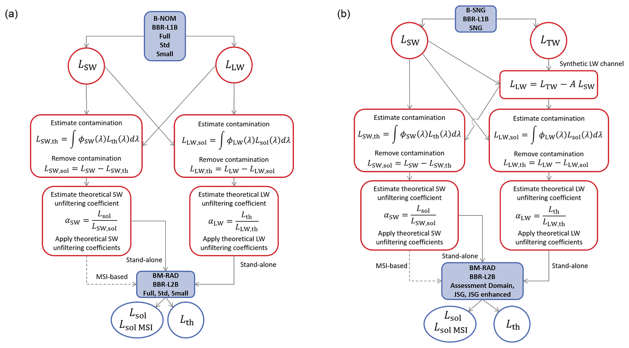
Figure 2Unfiltering flow chart for the BM-RAD product on the BBR grid resolutions (full, standard, and small) from the level-1 B-NOM (a) and the on the JSG grid resolutions (assessment, JSG, and JSG enhanced) from the level-1 B-SNG product (b).
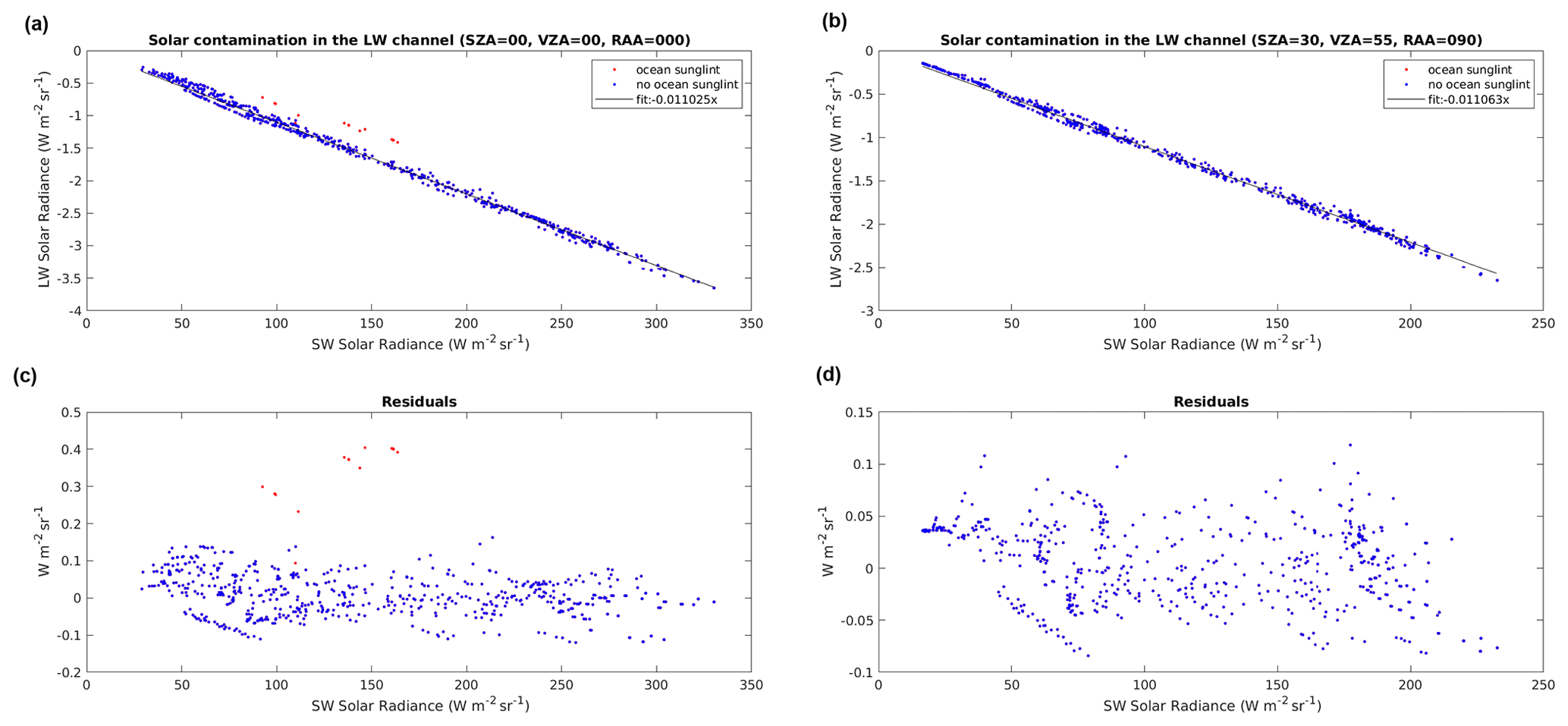
Figure 3Solar contamination in the LW channel. Represented here is the contamination for (a) the nadir view of the BBR for a sunglint geometry (SZA = 0°, VZA = 0°, RAA = 0°), (b) the off-nadir view for a non-sunglint geometry (SZA = 30°, VZA = 55°, RAA = 90°), (c) the residuals of the fit for the nadir view in (a), and (d) residuals for the off-nadir view in (b).
The unfiltering factors and the contaminations are obtained theoretically from two large geophysical databases: one of reflected solar radiances containing 5544 simulations Lsol(λ), i.e. 616 unique scenes simulated at nine solar zenith angles (SZAs), and one of Earth's emitted thermal radiances containing 12 096 simulations Lth(λ). The solar simulations Lsol(λ) are performed for nine SZAs, from 0 to 80° in steps of 10°, and the simulated radiance field is extracted at 18 viewing zenith angles (VZAs), 0 to 85° every 5°, and 19 relative azimuth angles (RAAs), 0 to 180° every 10°. These databases are computed using the libRadtran 1.4 (Mayer and Kylling, 2005) radiative transfer model as described in Velazquez et al. (2010). The simulations cover a wide range of geophysical conditions, and for this purpose, the scene definition has been done using ancillary models and data, such as surface reflectances from the Aster Spectral Library data (Baldridge et al., 2009) and the Optical Properties of Aerosols and Clouds (OPAC) software (Hess et al., 1998) for the computation of the aerosol optical properties. The aerosols are assumed to be well mixed and defined as being in the mixing layer, between 0 and 6 km for desert aerosols and between 0 and 2 km for continental and maritime aerosols. Given that the Aster Spectral Library contains a large number of spectra, a k-means clustering of 12 clusters has been done for clear-sky scenes. An averaging of the spectra has been done for those scenes with presence of aerosols. The simulations completely cover the illumination and observation geometries of EarthCARE. Various types of clouds have been simulated with optical thickness from 0.3 to 300 and altitudes ranging from 1 to 12 km. The standard profiles used for the simulations are tropical, midlatitude summer, midlatitude winter, subarctic summer, and subarctic winter (Anderson et al., 1986). Scaling (factor between 0.6 and 1.4) of the water vapour profile in the LW simulations is done to take into account the variability of the water vapour.
Solar simulations have been done in the interval of 0.25 to 5 µm, for 833 wavelengths, with the following spectral resolution: from 0.25 to 1.36 µm in steps of 0.002 µm, from 1.36 to 2.5 µm in steps of 0.005 µm, and from 2.5 to 5 µm in steps of 0.05 µm. Thermal simulations have been done in the interval of 2.5 to 100 µm, for 762 wavelengths, with the following spectral resolution: from 2.5 to 14 µm in steps of 0.05 µm, from 14.1 to 50 µm in steps of 0.1 µm, and from 55 to 100 µm in steps of 0.5 µm. The limit at 100 µm for the simulations is due to the fact that ice and water cloud properties are defined up to this wavelength for both the Yang (Yang et al., 2000) (ice crystals) and Mie (water droplets) parameterizations. As there is still significant radiation beyond 100 µm, the longwave simulations Lth(λ) have been extrapolated up to λ=500 µm using the black body emission curve corresponding to the brightness temperature simulated at λ=100 µm as in Clerbaux et al. (2008b).
The simulated radiances L(λ) are convoluted with the SW, TW, and LW spectral responses ϕ(λ) of the BBR for each of the views (fore, nadir, aft) to obtain the filtered radiances for each geometry. The unfiltered radiances are obtained with a perfect constant “filter” ϕ(λ)=1.
4.1 Flow charts
In the level-1 B-NOM product, the SW- and LW-filtered radiances are provided over areas defined according to the instrument grid (the BBR grid). These domains are the standard, small, and full integration domains. The level-2 BM-RAD products are then provided at the same domains as the level-1 input. The processing flow chart is given in the left panel of Fig. 2. Firstly, the solar contamination in the LW channel and the thermal contamination in the SW channel are estimated and subtracted from the filtered LW- and SW-filtered radiances, respectively. In this way purely thermal and solar radiances are obtained. Secondly, the unfiltering factors are estimated and applied to obtain the unfiltered thermal and solar radiances. The level-1 B-SNG product provides measurements of the SW and TW radiation at detector level. The B-SNG file is the main input to compute the level-2 BM-RAD products over the assessment domain (AD), which is defined on the mission Joint Standard Grid (JSG). Among the different resolutions, the AD is especially important as the EarthCARE radiative computations products (Cole et al., 2023) will be evaluated on this domain. The flow chart is shown in the right panel of Fig. 2, which also shows the additional estimation of the synthetic LW radiance.
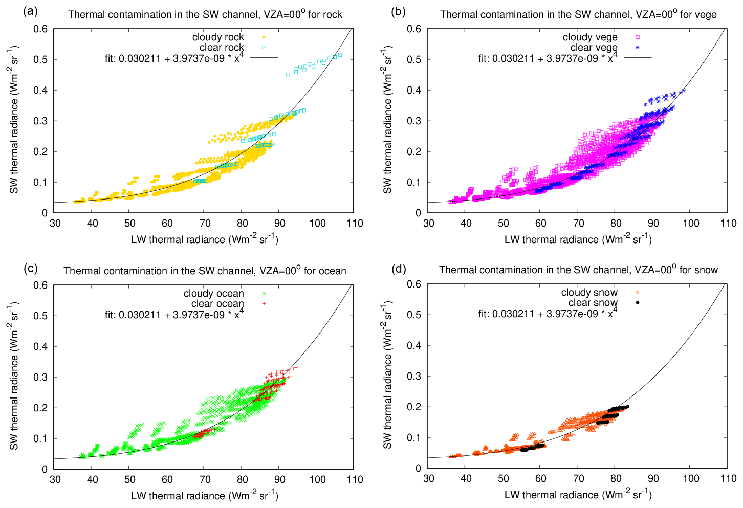
Figure 4Thermal contamination in the SW channel for rock (a), vegetation (b), ocean (c), and snow (d) surfaces. Represented here is the contamination for the nadir view of the BBR. Very similar scatter plots, not shown, exist for the fore and aft views. The polynomial fit shown in the figure is independent of the surface type and cloudiness. For each plot, a different colour is used to show the clear and cloudy simulations.
Two algorithms have been developed for the shortwave: the “stand-alone” unfiltering that relies only on the BBR observations and the “MSI-based” unfiltering in which cloud mask and cloud phase information from the MSI is used as additional information to improve the accuracy of the unfiltering. In the stand-alone algorithm, the regression coefficients are dependent on the geometry and surface type while in the MSI-based algorithm they are also dependent on the cloud mask, cloud phase, and snow information from X-MET. For the LW, only a stand-alone algorithm is implemented, as the unfiltering performs well within the requirements.
4.2 Solar contamination in the LW channel
Figure 3 shows the scatter plots of the solar contamination in the LW channel, LLW,sol, as a function of the solar radiances, LSW,sol, for the four different surface types (rock, vegetation, ocean, and snow) and for clear and cloudy conditions. Each dot corresponds to one simulation in the libRadtran database. The figures illustrate two particular sun–target–satellite geometries, a sunglint case for the nadir view (SZA = 0°, VZA = 0°, RAA = 0°) and a non-sunglint case for the off-nadir views (SZA = 30°, VZA = 55°, RAA = 90°). The contamination of the synthetic LW channel with solar radiation is negative (as expected, as the synthetic LW response is negative in the shortwave region) and shows a linear relationship with the intensity of the solar radiation. Therefore, the contamination can be estimated as follows:
where the factor acont_LW is dependent on the geometry (SZA, VZA, RAA) but not on the surface type or the cloudiness. Flat ocean scenes corresponding to sunglint situations have not been considered in the fit (i.e., scenes with sunglint angle lower than 10° and wind speed that is equal to or lower than 1 m s−1) as with the three BBR views it will be possible to reduce the sunglint effects as the three telescopes will not be subject to sunglint at the same time. The residual RMSE of the regression averaged for all the VZAs in the database is 0.034 , which is acceptable for a typical signal in the LW channel ( 60 ). Higher errors are expected for sunglint scenes, in which the error is estimated to be about 0.5 for a typical ocean clear-sky LW radiance of 80 .
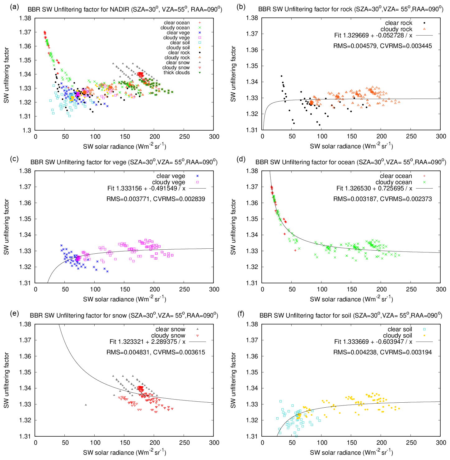
Figure 5Stand-alone SW unfiltering for all scenes together (a) and then separated according to the surface type (rock (b), vegetation (c), ocean (d), snow (e), and soil (f)). These graphs are for the (SZA = 30°, VZA = 55°, RAA = 90°) geometry, representative of the fore and aft views. Similar graphs exist for the nadir view (not shown).
4.3 Thermal contamination in the SW channel
Figure 4 shows the scatter plots of the thermal contamination, LSW,th, as a function of the thermal radiances, LLW,th, for four different surface types (rock, vegetation, ocean, and snow) and for clear and cloudy conditions. This figure constructed for VZA = 0° is representative of the nadir view telescope of the BBR. The LSW,th contamination increases more than linearly with respect to the scene thermal radiance, which is due to the shift of the Planck emission towards shorter wavelengths when the temperature increases. A good fit is obtained with the following relationship:
in which the regression coefficients acont_SW and bcont_SW are dependent on the VZA but not on the surface or cloudiness types.
For the 12 096 scenes in the LW database, the contamination in the SW channel is lower than 0.6 . The feather shape and variability in the LW thermal range come from the wide range of water content in the water vapour profiles simulated in the LW database. Higher errors in the estimation of the contamination are expected for very warm scenes like bright desert scenes and for scenes with a high water vapour content in warm atmospheres (e.g., tropical and midlatitude summer). Ice phase high clouds (at 12 km in the simulations) also show higher errors than the rest of scenes. The residual RMSE on the estimation of the contamination, averaged over all the geometries in the database (VZA from 0 to 85° in steps of 5°), is 0.016 , which is acceptable with respect to a typical signal in the SW channel of 100 .
4.4 Stand-alone SW unfiltering
A first unfiltering algorithm that does not rely neither on the MSI radiances nor on cloud products has been developed. In the flow chart of Fig. 2 this step corresponds to the αSW estimation boxes. The motivation behind this is to enable the BBR data to be unfiltered even if the MSI observations are unavailable or if they become degraded with time. In addition, the stand-alone unfiltering algorithm may be useful to assess the problems introduced by the cloud parallax between the fore and aft views and the MSI nadir observation of the scene. An example of the distribution of the unfiltering factors is given in Fig. 5 (top left panel) for a given geometry (SZA = 30°, VZA = 55°, RAA = 90°) representative of the fore and aft views.
The other panels in Fig. 5 show the same data but separated according to the surface type (rock, vegetation, ocean, snow and soil). For most of the surface types, the best fit is obtained with the hyperbolic equation:
which is identical to the relation used for the CERES (Loeb et al., 2001) and GERB (Clerbaux et al., 2008a) shortwave channels. It is worth mentioning that the CERES team is currently reviewing its unfiltering process, and several improvements are proposed in Liang et al. (2024) for possible inclusion in Edition 5. Those improvements concern mostly the use of the Cox–Munk ocean BRDF, MODIS BRDF over land, seasonal variations of the vegetation, a finer angular resolution, and the use of MODTRAN 5.2 for the radiative transfer simulations. Future versions of the BBR unfiltering could potentially benefit from this revision of the original CERES Unfiltering.
.
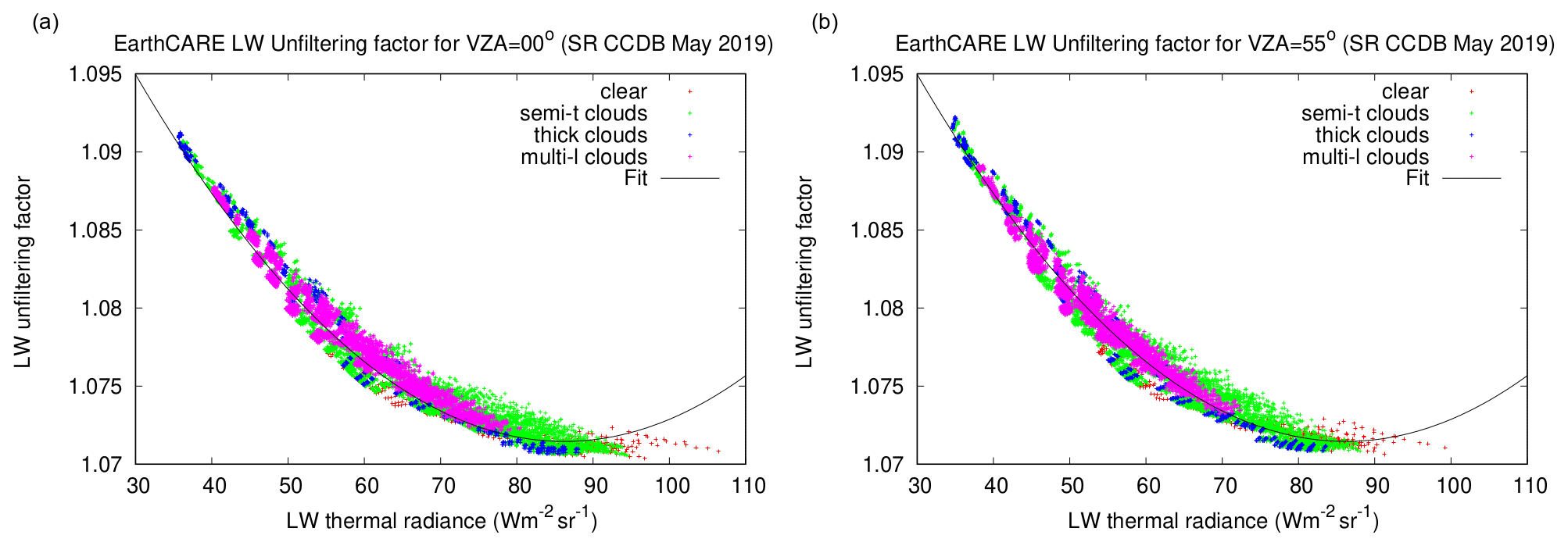
Figure 6Scatter plot of unfiltering factors for the LW channel of the BBR (see Eq. 18), for (a) VZA = 0° and (b) VZA = 55°.
The regression coefficients aSW and bSW are dependent on the surface type and on the viewing and solar geometries. The residual RMSE of the fit is provided in the different panels of Fig. 5. The typical RMSE of 0.004 corresponds to about 0.3 % relative error on the unfiltering factor αSW and thus also to 0.3 % on the unfiltered radiance Lsol and later also on the solar flux Fsol.
4.5 MSI-based SW unfiltering
The objective of this scene dependent unfiltering is to further reduce the unfiltering error (evaluated at 0.3 % at 1 standard deviation for the stand-alone, see previous section) using explicit information about the scene type within the BBR domains (standard, small, full, or assessment domain). The study is similar to the stand-alone one, but the regressions (see Eq. 17) are in this case also dependent on the cloud mask (clear or cloudy condition) and the cloud phase (water droplets or ice crystals). Although the MSI-based algorithm provides slightly better results in the validation than the stand-alone algorithm (plots not shown in the text), its applicability to the fore and aft views might be affected by cloud parallax effects, as the MSI provides a nadir view of the scene. Table 2 presents the results obtained for test scenes in comparison with the results derived from the stand-alone approach. The applicability of the MSI-based algorithm will be tested during the commissioning phase once real data are available.
4.6 LW unfiltering
The LW channel unfiltering is illustrated in Fig. 6 which shows the scatter plots of the unfiltering factor αlw versus the longwave thermal radiance Lth,lw, for the nadir view (left panel) and the VZA = 55° views (right panel). The range of variability of the LW unfiltering factor for the BBR instrument is very reduced and much smaller than for the CERES and GERB instruments. The primary reason for this is that the BBR optics only has one mirror, while CERES has two, and GERB has five. A second degree polynomial fit in the scatter plots appears suitable to estimate the unfiltering coefficients:
where the coefficients aLW, bLW, and cLW are dependent on the VZA. For clear-sky warm scenes, the LW unfiltering factor presents enhanced variability due to variability in the spectral emissivity of the desert surfaces. Even though the performance of a single regression, with a rms of about 0.1 %, is sufficient with respect to the scientific requirements of the mission, it was investigated if any improvement could be obtained using specific regressions for ocean, vegetation, and desert surfaces. The improvement of using surface type dependent regressions is negligible and is therefore not further considered.
An analysis of the unfiltering error is performed for 10 typical scene types covering the full extent in terms of SW and LW radiances. The error combines the one due to the estimation of the contamination and the error due to the estimation of the unfiltering factor. The results are summarized in Table 1 and provide values averaged over the full range of simulated SZA, VZA, and RAA geometries. For the solar radiation, the relative error on the unfiltered radiances is ≈0.26 % for cloudy conditions and increases up to 0.34 % for clear-sky conditions. For the thermal radiation, the relative error is 0.10 ± 0.02 % for all of scene conditions.
Table 1BBR unfiltering error analysis for 10 scene types (first column). For each scene type, the columns give the number of libRadtran simulations in the solar database, the averaged solar radiance , and the RMSE on this radiance due to the subtraction of the thermal contamination and the error due to the unfiltering of the shortwave channel. The RMSE is expressed as an absolute value, in , and also as a relative error, in percent. The last four columns provide the results for the unfiltering of the LW channel. Averaged values have been calculated over all the observation and illumination geometries, i.e., SZA [0:10:80], VZA [0:5:85], and RAA[0:10:180].
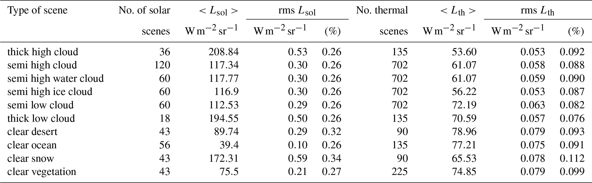
Table 2Statistics of the BBR unfiltering errors for the three test scenes (Halifax, Baja, Hawaii) and each of the three views of the BBR (fore, nadir, aft). The upper parts of the table provide the errors for the stand-alone and MSI-based unfiltering of the SW channel. The bottom part is for the (stand-alone) unfiltering of the longwave channel.
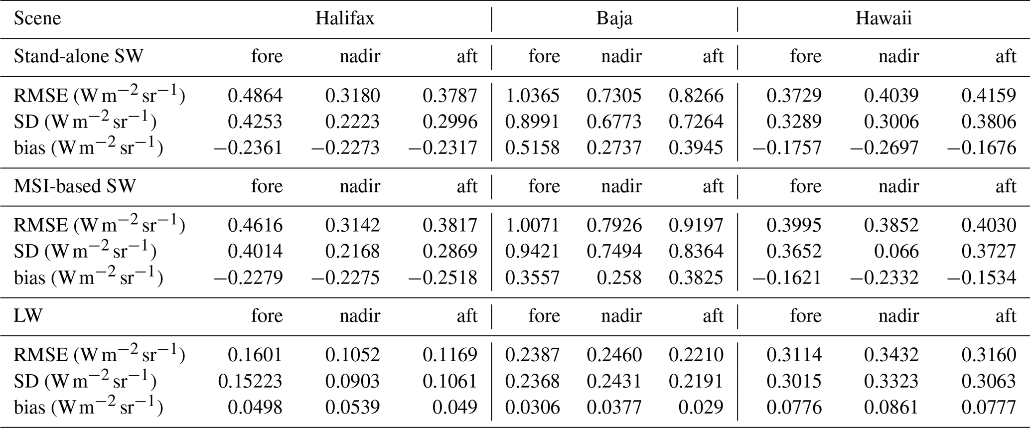
In this section, data from the three EarthCARE test frames (Qu et al., 2023; Donovan et al., 2023) have been used to verify the performances of the BM-RAD processor. In general a close agreement is found between the unfiltered radiances calculated by the BM-RAD processor and the reference radiances (truth) obtained directly by broadband integration of the radiative transfer computations on the Global Environmental Multiscale Model (GEM) scenes. Table 2 details the results in terms of bias, rms, and standard deviation, all expressed in ; these are for the three telescopes (fore, nadir, aft) and for the three test frames (Halifax, Baja, Hawaii).
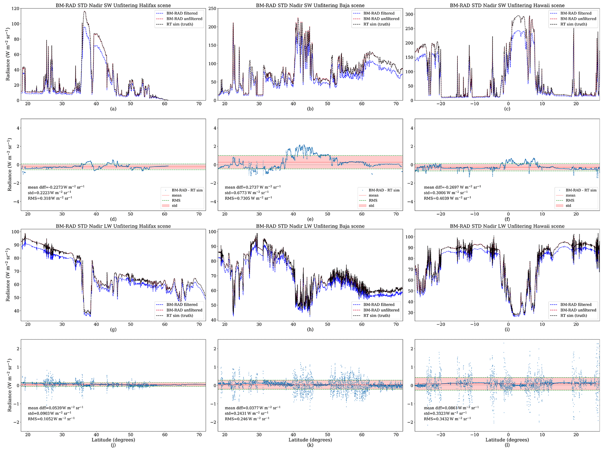
Figure 7Filtered and unfiltered radiances versus the radiative transfer simulations “RT sim (truth)” across the three test scenes of Halifax (a, g), Baja (b, h), and Hawaii (c, i). Panels (a), (b), and (c) show the shortwave radiances along the satellite track (and goes to zero in night time condition). Panels (g), (h), and (i) show the corresponding results for the longwave radiation. The difference between the BM-RAD unfiltered solar radiance and the reference value is shown in (d), (e), and (f), and the corresponding differences for the thermal radiances are shown in (j), (k), and (l). The graphs shown here correspond to the nadir view. Similar results are obtained for the off-nadir views (not shown).
Table 2 summarizes the performances of the stand-alone SW unfiltering, MSI-based SW unfiltering, and stand-alone LW unfiltering procedures for the three test scenes. The error metrics show that the MSI-based shortwave unfiltering provides a small improvement in general. The gaining of including MSI information in the unfiltering process while improving results might not be very large in practice because of parallax effects. Another interesting finding is that the unfiltering of the nadir view is, in general, more accurate than the one of the fore and aft views (with, however, an exception for the stand-alone shortwave unfiltering for the Hawaii scene).
The upper panels of Fig. 7 show the filtered, unfiltered, and simulated (truth) radiances along the orbit frame for the three test scenes. Differences between filtered and unfiltered radiances can be clearly seen. As expected, the greatest differences are observed over cloudy scenes in the SW regime, while clear-sky scenes present the higher differences in the thermal radiances. Lower panels show the detail of the differences between the unfiltered radiances and the truth radiance. The corresponding mean difference (bias), standard deviation, and RMSE are provided to quantitatively analyse the comparison. The complete summary of results is available in Table 2. The RMSEs for both SW and LW unfiltered radiances are well within the accuracy requirement for the BBR that is 2.5 for the SW and 1.5 for the LW. It is worth mentioning that these metrics are likely an overestimation of the errors because of the simplifications needed in the radiative transfer computations used for the construction of the test scenes.
In this paper, the algorithms used by the unfiltering processor (BM-RAD) for the BBR instrument on board EarthCARE are described. The main output of BM-RAD is the unfiltered solar and thermal radiances for the three BBR views integrated over different spatial domains. These radiances are the main input for the BMA-FLX processor in which the three views are combined to estimate the hemispheric outgoing shortwave and longwave radiative fluxes.
Thanks to its design, the BBR instrument sensitivity shows limited spectral variability, which is a prerequisite for an accurate unfiltering process. The typical stand-alone unfiltering errors are expected to be approximately 0.5 % for the shortwave channel and well below 0.1 % for the longwave channel. The implementation of the algorithm has been successfully verified on the three EarthCARE test scenes (Halifax, Baja, and Hawaii).
Scene information from the MSI radiances (from M-RGR product), MSI cloud retrievals (from M-CLD processor), or snow products (from X-MET product) is useful to further reduce the unfiltering error. So, in addition to the stand-alone unfiltered radiances, the BM-RAD product also contains the MSI-based unfiltered radiance for the shortwave radiation (the improvement for the longwave radiance was considered negligible and therefore not included in the product). However, the MSI-based unfiltering of the fore and aft views might suffer from the parallax effect as the MSI only provides nadir observations. Therefore, a comprehensive evaluation of the MSI-based unfiltering is foreseen to be carried out during the commissioning phase, when the BM-RAD processor can be applied on real BBR and MSI observations. In the meantime, the stand-alone unfiltered radiances should be used.
The EarthCARE demonstration products from the simulated scenes, including B-NOM and B-SNG L1 data and the BM-RAD L2 products, discussed in this paper are available from https://doi.org/10.5281/zenodo.7728948 (van Zadelhoff et al., 2023). The radiative transfer simulation database and description are available at https://gerb.oma.be/public/almudena/SITS_DB_compressed/ (Velazquez et al., 2010).
The manuscript was prepared by AVB, EB, NC, and CD. The BM-RAD software was developed by AVB, EB, and NC.
The contact author has declared that none of the authors has any competing interests.
Publisher’s note: Copernicus Publications remains neutral with regard to jurisdictional claims made in the text, published maps, institutional affiliations, or any other geographical representation in this paper. While Copernicus Publications makes every effort to include appropriate place names, the final responsibility lies with the authors.
This article is part of the special issue “EarthCARE Level 2 algorithms and data products”. It is not associated with a conference.
We express our deepest gratitude to Tobias Wehr, who sadly passed away on 1 February 2023, for his continuous support, contagious positivism, and endless discussions. EarthCARE would not have been possible without the contributions of Tobias Wehr.
This research has been supported by the European Space Agency (ESA contract nos. 4000112019/14/NL/CT (CLARA) and 4000134661/21/NL/AD (CARDINAL)).
This paper was edited by Robin Hogan and reviewed by two anonymous referees.
Anderson, G. P., Clough, S. A., Kneizys, F. X., Chetwynd, J. H., and Shettle, E. P.: AFGL atmospheric constituent profiles (0- 120 km). AFGL-TR; 86-0110, Air Force Geophysics Laboratory, Air Force Systems Command, United States Air Force, Hanscom AFB, Massachusetts, https://ntrl.ntis.gov/NTRL/dashboard/searchResults/titleDetail/ADA175173.xhtml# (last access: 2 July 2024), 1986.
Baldridge, A., Hook, S., Grove, C., and Rivera, G.: The ASTER Spectral Library Version 2.0, Remote Sens. Environ., 113, 711–715, 2009. a
Barker, H. W., Cole, J. N. S., Villefranque, N. Qu, Z., Velázquez Blázquez, A., Domenech, C., Mason, S., and Hogan, R.: Radiative closure assessment of retrieved cloud and aerosol properties for the EarthCARE mission: The ACMB-DF product, Atmos. Meas. Tech., submitted, 2024. a
Clerbaux, N.: Processing of Geostationary Satellite Observations for Earth Radiation Budget Studies, PhD thesis, Vrije Universiteit Brussel (VUB), https://gerb.oma.be//people/gerb/clerbaux_thesis.pdf (last access: 27 May 2024), 2008. a
Clerbaux, N., Dewitte, S., Bertrand, C.and Caprion, D., De Paepe, B., and Ipe, A.: Unfiltering of the Geostationary Earth Radiation Budget (GERB) Data. Part I: Shortwave Radiation, J. Atmos. Ocean. Tech., 25, 1087–1105, 2008a. a
Clerbaux, N., Dewitte, S., Bertrand, C., Caprion, D., De Paepe, B., and Ipe, A.: Unfiltering of the Geostationary Earth Radiation Budget (GERB) Data. Part II: Longwave Radiation, J. Atmos. Ocean. Tech., 25, 1106–1117, 2008b. a
Cole, J. N. S., Barker, H. W., Qu, Z., Villefranque, N., and Shephard, M. W.: Broadband radiative quantities for the EarthCARE mission: the ACM-COM and ACM-RT products, Atmos. Meas. Tech., 16, 4271–4288, https://doi.org/10.5194/amt-16-4271-2023, 2023. a
Donovan, D. P., Kollias, P., Velázquez Blázquez, A., and van Zadelhoff, G.-J.: The generation of EarthCARE L1 test data sets using atmospheric model data sets, Atmos. Meas. Tech., 16, 5327–5356, https://doi.org/10.5194/amt-16-5327-2023, 2023. a
Eisinger, M., Marnas, F., Wallace, K., Kubota, T., Tomiyama, N., Ohno, Y., Tanaka, T., Tomita, E., Wehr, T., and Bernaerts, D.: The EarthCARE mission: science data processing chain overview, Atmos. Meas. Tech., 17, 839–862, https://doi.org/10.5194/amt-17-839-2024, 2024. a
Helière, A., K., W., Pereira do Carmo, J.and Eisinger, M., Wehr, T., and Lefebvre, A.: EarthCARE Instruments Description 1.0. EC-TN-ESA-SYS-0891, Tech. rep., ESA, https://earth.esa.int/eogateway/documents/20142/37627/EarthCARE-instrument-descriptions.pdf (last access: 27 May 2024), 2017. a
Hess, M., Koepke, P., and Schult, I.: Optical properties of aerosols and clouds: the software package OPAC, B. Am. Meteorol. Soc., 79, 831–844, 1998. a
Hünerbein, A., Bley, S., Horn, S., Deneke, H., and Walther, A.: Cloud mask algorithm from the EarthCARE Multi-Spectral Imager: the M-CM products, Atmos. Meas. Tech., 16, 2821–2836, https://doi.org/10.5194/amt-16-2821-2023, 2023. a
Illingworth, A. J., Barker, H. W., Beljaars, A., Ceccaldi, M., Chepfer, H., Clerbaux, N., Cole, J., Delanoë, J., Domenech, C., Donovan, D. P., Fukuda, S., Hirakata, M., Hogan, R. J., Huenerbein, A., Kollias, P., Kubota, T., Nakajima, T., Nakajima, T. Y., Nishizawa, T., Ohno, Y., Okamoto, H., Oki, R., Sato, K., Satoh, M., Shephard, M. W., Velázquez-Blázquez, A., Wandinger, U., Wehr, T., and van Zadelhoff, G.-J.: The EarthCARE Satellite: The Next Step Forward in Global Measurements of Clouds, Aerosols, Precipitation, and Radiation, B. Am. Meteorol. Soc., 96, 1311–1332, https://doi.org/10.1175/BAMS-D-12-00227.1, 2015. a
Liang, L., Su, W., Sejas, S., Eitzen, Z., and Loeb, N. G.: Next-generation radiance unfiltering process for the Clouds and the Earth's Radiant Energy System instrument, Atmos. Meas. Tech., 17, 2147–2163, https://doi.org/10.5194/amt-17-2147-2024, 2024. a
Loeb, N., Priestley, K., Kratz, D., Geier, E., Green, R., Wielicki, B., Hinton, P., and Nolan, S.: Determination of Unfiltered Radiances from the Clouds and the Earth's Radiant Energy System instrument, J. Appl. Meteorol., 40, 822–835, 2001. a
Mayer, B. and Kylling, A.: Technical note: The libRadtran software package for radiative transfer calculations – description and examples of use, Atmos. Chem. Phys., 5, 1855–1877, https://doi.org/10.5194/acp-5-1855-2005, 2005. a
Proulx, C., Allard, M., Pope, T., Tremblay, B., Williamson, F., Delderfield, J., and Parker, D.: EarthCARE BBR detectors performance characterization, in: Sensors, Systems, and Next-Generation Satellites XIV, edited by: Meynart, R., Neeck, S. P., and Shimoda, H., vol. 7826, International Society for Optics and Photonics, SPIE, 498–508, https://doi.org/10.1117/12.868518, 2010. a
Qu, Z., Donovan, D. P., Barker, H. W., Cole, J. N. S., Shephard, M. W., and Huijnen, V.: Numerical model generation of test frames for pre-launch studies of EarthCARE's retrieval algorithms and data management system, Atmos. Meas. Tech., 16, 4927–4946, https://doi.org/10.5194/amt-16-4927-2023, 2023. a
Spilling, D. and Wright, N.: ECGP Algorithm Theoretical Baseline Document, EC-TN-SEA-BBR-0005, Tech. rep., 2020. a
van Zadelhoff, G.-J., Barker, H. W., Baudrez, E., Bley, S., Clerbaux, N., Cole, J. N. S., de Kloe, J., Docter, N., Domenech, C., Donovan, D. P., Dufresne, J.-L., Eisinger, M., Fischer, J., García-Marañón, R., Haarig, M., Hogan, R. J., Hünerbein, A., Kollias, P., Koopman, R., Madenach, N., Mason, S. L., Preusker, R., Puigdomènech Treserras, B., Qu, Z., Ruiz-Saldaña, M., Shephard, M., Velázquez-Blázquez, A., Villefranque, N., Wandinger, U., Wang, P., and Wehr, T.: EarthCARE level-2 demonstration products from simulated scenes, Zenodo [data set], https://doi.org/10.5281/zenodo.7728948, 2023. a
Velázquez, A., Clerbaux, N., Brindley, H., Dewitte, S., Ipe, A., and Russel, J.: Index of /public/almudena/SITS_DB_compressed, gerb.oma.be [data set], https://gerb.oma.be/public/almudena/SITS_DB_compressed/ (last access: 15 July 2024), 2010. a, b
Velázquez Blázquez, A., Domenech, C., Baudrez, E., Clerbaux, N., Salas Molar, C., and Madenach, N.: Retrieval of top-of-atmosphere fluxes from combined EarthCARE LiDAR, imager and broadband radiometer observations: the BMA-FLX product, EGUsphere [preprint], https://doi.org/10.5194/egusphere-2024-1539, 2024. a
Wallace, K., Wright, N., Spilling, D., Ward, K., and Caldwell, M.: The broadband radiometer on the EarthCARE spacecraft, Proc. SPIE, Infrared Spaceborne Remote Sensing and Instrumentation XVII, San Diego, California, United States, 2 September 2009, vol. 7453, https://doi.org/10.1117/12.825837, 2009. a
Wehr, T., Kubota, T., Tzeremes, G., Wallace, K., Nakatsuka, H., Ohno, Y., Koopman, R., Rusli, S., Kikuchi, M., Eisinger, M., Tanaka, T., Taga, M., Deghaye, P., Tomita, E., and Bernaerts, D.: The EarthCARE mission – science and system overview, Atmos. Meas. Tech., 16, 3581–3608, https://doi.org/10.5194/amt-16-3581-2023, 2023. a
Yang, P., Liou, K., Wyser, K., and Mitchell, D.: Parameterization of the scattering and absorption properties of individual ice crystals, J. Geophys. Res., 105, 4699–4718, https://doi.org/10.1029/1999JD900755, 2000. a
- Abstract
- Introduction
- BBR spectral responses and unfiltering problem statement
- Radiative transfer simulations
- The BM-RAD algorithm
- BM-RAD algorithm verification
- End-to-end verification of the algorithm using test scenes
- Conclusions
- Data availability
- Author contributions
- Competing interests
- Disclaimer
- Special issue statement
- Acknowledgements
- Financial support
- Review statement
- References