Quantitative estimate of several sources of uncertainty in drone-based methane emission measurements

Site-level measurements of methane emissions are used by operators for reconciliation with bottom-up emission inventories with the aim to improve accuracy, thoroughness, and confidence in reported emissions. In that context it is of critical importance to avoid measurement errors and to understand the measurement uncertainty. Remotely piloted aircraft systems (commonly referred to as “drones”) can play a pivotal role in the quantification of site-level methane emissions. Typical implementations use the “mass balance method” to quantify emissions, with a high-precision methane sensor mounted on a quadcopter drone flying in a vertical curtain pattern; the total mass emission rate can then be computed post hoc from the measured methane concentration data and simultaneous wind data. Controlled-release tests have shown that errors with the mass balance method can be considerable. For example, Liu et al. (2024) report absolute errors for more than 100 % for the two drone solutions tested; on the other hand, errors can be much smaller, of the order of 16 % root-mean-square errors in Corbett and Smith (2022), if additional constraints are placed on the data, restricting the analysis to cases where the wind field was steady. In this paper we present a systematic error analysis of physical phenomena affecting the error in the mass balance method for parameters related to the acquisition of methane concentration data and to postprocessing. The sources of error are analyzed individually, and it must be realized that individual errors can accumulate in practice, and they can also be augmented by other sources that are not included in the present work. Examples of these sources include the uncertainty in methane concentration measurements by a sensor with finite precision or the method used to measure the unperturbed wind velocity at the position of the drone. We find that the most important source of error considered is the horizontal and vertical spacings in the data acquisition, as a coarse spacing can result in missing a methane plume. The potential error can be as high as 100 % in situations where the wind speed is steady and the methane plume has a coherent shape, contradicting the intuition of some operators in the industry. The likelihood of the extent of this error can be expressed in terms of a dimensionless number defined by the spatial resolution of the methane concentration measurements and the downwind distance from the main emission sources. What is learned from our theoretical error analysis is then applied to a number of historical measurements in a controlled-release setting. We show how what is learned about the main sources of error can be used to eliminate potential errors during the postprocessing of flight data. Second, we evaluate an aggregated data set of 1001 historical drone flights; our analysis shows that the potential errors in the mass balance method can be of the order of 100 % on occasion, even though the individual errors can be much smaller in the vast majority of the flights. The Discussion section provides some guidelines for industry on how to avoid or minimize potential errors in drone measurements for methane emission quantification.

1 Introduction

Methane is a much more potent greenhouse gas than carbon dioxide when comparing global warming potential (GWP). Methane has a GWP of 86 over the first 20 years after its atmospheric injection and a GWP of 28 over a 100-year time frame (IPCC, 2014). Since the lifetime of methane in the atmosphere is just over 12 years (relatively short compared to CO₂’s lifetime of hundreds of years), reducing methane emissions now offers great potential for delivering substantial reductions in global warming on a timescale compatible with the 2015 Paris Agreement goals. The average background level of methane in the atmosphere is about 1.9 ppm globally, increasing at about 0.01 ppm yr⁻¹ due to human activity (Nisbet et al., 2019). According to bottom-up estimates over the period 2008–2017 by Saunois et al. (2020), about half of the total methane emission sources are anthropogenic (366 Tg yr⁻¹ out of 737 Tg yr⁻¹), predominantly from agriculture and waste (206 Tg yr⁻¹); oil and gas production accounts for 22 % of total anthropogenic emissions (80 Tg yr⁻¹). Although all these numbers are subject to high uncertainty, the estimates do show that reducing methane emissions from the oil and gas industry can have a significant effect on limiting climate change in the coming decades.

Best practices for the reporting of methane emissions are proposed in the OGMP2.0 reporting framework (United Nations Environment Programme, 2020) – a voluntary, comprehensive, measurement-based reporting framework for the oil and gas industry. At the highest reporting level OGMP2.0 recommends building a measurement-based source-level inventory of emissions and performing an independent site-level emission measurement – as well as a reconciliation of the two. The aim of reconciliation is to help improve accuracy in reported emissions as well as identifying emission reduction opportunities. In this context it is important for operators to understand sources of error and uncertainty ranges in measurement techniques used. Sources of measurement errors should be avoided where possible and practical, and remaining uncertainties should be understood and correctly estimated. Site-level quantification is typically done with airborne methane measurements (e.g., on remotely piloted aircraft systems or on crewed aircraft). Liu et al. (2024) note that the errors in quantification can be considerable: although many systems can quantify within an order of magnitude of the controlled-release rate, the absolute errors reported varied between 19 % and 239 %. The two remotely piloted aircraft systems (drones) tested even reported results with errors of 140 % and 239 %. Corbett and Smith (2022) present the results from another controlled-release campaign: they report errors in the methane emission rate up to 115 %, but they also show that the errors can be much reduced, to about 16 %, by considering only measurements during the time that the wind conditions were favorable. Still, Corbett and Smith (2022) do not give a systematic analysis of the causes as to why some measurements are more successful than others.

The present paper provides a framework that allows the quantitative assessment of errors in methane emission rate measurements using the mass balance method. We present a theoretical framework that provides an explanation for the various sources of uncertainty considered and that highlights which of these effects have a particularly large impact on uncertainty – and thus are those effects that should be managed most carefully when setting up a drone survey campaign. The focus will be on the uncertainty related to the flight path and the variability in the wind; we do not take into account additional uncertainty associated with the limited precision of the methane concentration sensor and the method used to determine the wind vector at the position of the drone (including anemometer precision).

The second part of this paper illustrates the various sources of uncertainty with real-life examples. Data from a controlled-release experiment acquired by Scientific Aviation are analyzed to illustrate potential uncertainties and subtleties associated with the data analysis process. In addition, a data set of 1001 historic flights acquired by SeekOps is analyzed with regards to the variations in the wind speed and direction during the survey time, as well as the potential effect of the choices for the drone’s flight path on the quality of the results.

This paper intends to provide guidelines to prevent avoidable errors in data collection and data analysis of drone-based measurements of methane emissions from industrial facilities. Although a number of obvious sources of potential error have been included in our analysis, it must be recognized that other errors may also occur in practice. This means that the actual uncertainty in measurement results will always depend on the particular deployment of a solution at a given site on a certain day. Examples of these additional sources of error are a reduced performance of the sensor(s) due to weather conditions or external damage, complications associated with turbulent air flow around buildings and pieces of equipment, and the method used to measure the unperturbed wind velocity at the position of the drone.

2 Methods

2.1 Coordinate system definition

Before describing the methods that are used for the quantification of methane emissions, we first introduce the coordinate systems that will be used in the remainder of this paper.

The first coordinate system is the local geodetic coordinate system (XYZ), with the X axis pointing to the east direction and the Y axis pointing to the north direction. The Z axis is defined such that a right-handed coordinate system is obtained.

The second coordinate system is aligned with the wind direction and referred to as ξηz. This means that the horizontal direction of the wind field is aligned with the ξ axis, the direction perpendicular to it is given by the η axis. The z axis is defined such that a right-handed system is obtained. The coordinate system is defined such that the emission source is located at ξ=0, η=0, and z=H, with H being the height of the source from the ground level (z=0) (see Fig. C2 in Appendix C).

The third coordinate system is defined to represent the drone measurements and is a 2-dimensional coordinate system that captures the trajectory flown by the drone. In the case of a “curtain” flight path (a vertical plane), each coordinate on the curtain is expressed in the Pz coordinate system, with the P axis parallel to the ground and the z axis in the vertical direction. In the case of cylindrical flight paths, polar coordinates θz are used, with z the vertical direction and θ the angular position in radians which can be converted to distance using the radius of the cylinder.

2.2 Mass balance method for methane emission quantification

The mass conservation equation for the methane mass concentration c (mass of methane per volume air) is (Stockie, 2011)

$$\begin{array}{}\text{(1)}& {\displaystyle \frac{\partial c}{\partial t}}+\mathbf{\nabla }\cdot \left(c\mathit{u}\right)=\mathbf{\nabla }\cdot \left(K\mathbf{\nabla }c\right)+\sum _i^{N_{\mathrm{sources}}}{\dot{m}}_i\mathit{\delta }(\mathit{x}-{\mathit{x}}_{s,i}),\end{array}$$

where u is the wind field vector and K is the molecular diffusivity of scalar c. The mass emission rate of point source i located at ${\mathit{x}}_{s,i}=[x_{s,i},y_{s,i},z_{s,i}]$ is denoted by ${\dot{m}}_i$; δ denotes the Dirac delta function. The first term on the left-hand side denotes the change in concentration in time, whereas the second term denotes the change due to advection; the first term on the right-hand side indicates molecular diffusion, and the second term accounts for the presence of point sources.

The methane mass concentration c is related to the molar volume of methane in air, c^′ [ppmv], through

$$\begin{array}{}\text{(2)}& c={\displaystyle \frac{c^{\prime }}{{\mathrm{10}}^{\mathrm{6}}}}\times {\displaystyle \frac{M_{{\mathrm{CH}}_{\mathrm{4}}}}{M_{\mathrm{air}}}}\times {\mathit{\rho }}_{\mathrm{air}},\end{array}$$

where $M_{{\mathrm{CH}}_{\mathrm{4}}}$ is the molar mass of methane (16.04 kg kmol⁻¹) and M_air is the molar mass of dry air (typically about 28.95 kg kmol⁻¹). The mass density of air, ρ_air, will change with differences in ambient temperature and pressure (i.e., ρ_air(T,P)).

We can obtain the mass balance equation for a volume by integrating:

$$\begin{array}{}\text{(3)}& \begin{array}{rl}& \underset{V}{\int }{\displaystyle \frac{\partial c}{\partial t}}\mathrm{d}V+\underset{V}{\int }\mathbf{\nabla }\cdot \left(c\mathit{u}\right)\mathrm{d}V=\underset{V}{\int }\mathbf{\nabla }\cdot \left(K\mathbf{\nabla }c\right)\mathrm{d}V+\\ & \underset{V}{\int }\sum _i^{N_{\mathrm{sources}}}{\dot{m}}_i\mathit{\delta }(\mathit{x}-{\mathit{x}}_{s,i})\mathrm{d}V,\end{array}\end{array}$$

where the integrals on both sides have units of kilograms per second. The total methane emission from all sources inside the volume combined can be estimated by applying the divergence theorem (Katz, 1979):

$$\begin{array}{}\text{(4)}& \dot{m}=\sum _i^{N_{\mathrm{sources}}}{\dot{m}}_i=\underset{V}{\int }{\displaystyle \frac{\partial c}{\partial t}}\mathrm{d}V+\underset{\partial V}{\oint }c\mathit{u}\cdot \mathit{n}\mathrm{d}S-\underset{\partial V}{\oint }K\mathit{n}\cdot \mathbf{\nabla }c\mathrm{d}S.\end{array}$$

Usually, the situation is considered where the main contribution on the right-hand side comes from the advection term (i.e., the wind vector is aligned with the normal vector n at the surface where the concentration flows out and $|c\mathit{u}\cdot \mathit{n}|\gg |K\mathit{n}\cdot \mathbf{\nabla }c|$ so that the diffusion term can be neglected; Conley et al., 2017). When the process is assumed to be statistically stationary (i.e., the statistical properties of the process do not change with time, $\frac{\partial c}{\partial t}$), it is possible to derive the mass balance equation (Conley et al., 2017) for the total methane emission rate:

$$\begin{array}{}\text{(5)}& \dot{m}\approx \underset{\partial V}{\oint }c\mathit{u}\cdot \mathit{n}\mathrm{d}S={\mathrm{10}}^{-\mathrm{6}}{\displaystyle \frac{M_{{\mathrm{CH}}_{\mathrm{4}}}}{M_{\mathrm{air}}}}\underset{\partial V}{\oint }{c}^{\prime }{\mathit{\rho }}_{\mathrm{air}}\mathit{u}\cdot \mathit{n}\mathrm{d}S,\end{array}$$

where the latter part is obtained by substituting Eq. (2).

We observe some inconsistencies in the presentation of the mass balance calculation in the existing literature, for instance with regards to the molar mass used (Corbett and Smith, 2022) or the distinction between concentrations by weight and by volume (Gorchov Negron et al., 2020). We hope to avoid further ambiguities through the full derivation of the mass balance method, leading up to Eq. (5).

2.3 Drone-based methane measurements

The relationship in Eq. (5) does not require that dispersion happens in a particular way (e.g., a Gaussian plume) or that there is only one source within the volume. To apply this form of the mass concentration equation to real problems, a flight path needs to be defined that approximates the boundary integral. In a common scenario, the measurements are taken downwind of an equipment area under the assumption that everything entering the upstream volume (behind the source) is atmospheric background, c₀. In some deployments, a cylindrical flight pattern is followed that circumscribes the facility of interest (Corbett and Smith, 2022).

The atmospheric background c₀ can be calculated statistically (e.g., some low percentile of the concentration measurements; McKain et al., 2015; Plant et al., 2022) or spatially (e.g., from grid cells at the edges of the plane; Mays et al., 2009; Conley et al., 2017). We use the former approach in this paper.

The terms inside the integral of Eq. (5) must generally be approximated, owing to the discrete nature of real concentration and wind measurements. We assume that the bounding surface (e.g., a cylinder or box around a region of interest or a plane downwind of a point of interest) can be partitioned into a 2-dimensional regular grid in the horizontal and vertical directions with equal spacings: δP and δz, respectively. The exact details of this grid will depend on the flight trajectory under consideration. Approximating Eq. (5) directly gives

$$\begin{array}{}\text{(6)}& \dot{m}\approx \sum _{k=\mathrm{1}}^{n_z}\sum _{j=\mathrm{1}}^{n_P}(c_{j,k}-c_{\mathrm{0}})[{\mathit{u}}_{j,k}\cdot {\mathit{n}}_{j,k}]\mathit{\delta }P\mathit{\delta }z,\end{array}$$

where c_j,k denotes the methane mass concentration and the wind field interpolated onto the grid at location x_j,k (either measured directly or interpolated onto a grid) and u_j,k denotes the wind field at the same location. n_j,k is the normal vector at the surface at location x_j,k. n_z and n_p are the number of cells in the P and z directions, respectively. For molar concentration measurements, the calculation should be modified to take account of the density of methane, as in Eq. (5):

$$\begin{array}{}\text{(7)}& \begin{array}{rl}& \dot{m}\approx {\mathrm{10}}^{-\mathrm{6}}{\displaystyle \frac{M_{\mathrm{CH}\mathrm{4}}}{M_{\mathrm{air}}}}\sum _{k=\mathrm{1}}^{n_z}\sum _{j=\mathrm{1}}^{n_P}(c_{j,k}^{\prime }-c_{\mathrm{0}}^{\prime }){\mathit{\rho }}_{\mathrm{air},\mathrm{j},\mathrm{k}}\left[{\mathit{u}}_{j,k}\cdot {\mathit{n}}_{j,k}\right]\\ & \mathit{\delta }P\mathit{\delta }z,\end{array}\end{array}$$

where ${\mathit{\rho }}_{\mathrm{air},j,k}$ represents the air density at the location x_j,k, which may be estimated using the local temperature and pressure.

Equations (6) and (7) describe the calculation procedure in the mass balance method for one single flight spanning the vertical plane of interest. If a similar trajectory along the vertical plane is flown multiple times, then the mass emission rate can be obtained by averaging. The exact choice of averaging procedure is important for the final result. Two common choices are as follows:

1. Find ${\dot{m}}_{\mathrm{\ell }}$ for each curtain ℓ separately using Eq. (7), and then take the average of these values following

   $$\begin{array}{}\text{(8)}& {\dot{m}}_{\mathrm{av},\mathrm{1}}={\displaystyle \frac{\mathrm{1}}{N_{\mathrm{curtain}}}}\sum _{\mathrm{\ell }=\mathrm{1}}^{N_{\mathrm{curtain}}}{\dot{m}}_{\mathrm{\ell }}.\end{array}$$

2. First compute the horizontal flux per altitude, ϕ_k, i.e., ${\mathit{\varphi }}_k={\mathrm{10}}^{-\mathrm{6}}\frac{M_{{\mathrm{CH}}_{\mathrm{4}}}}{M_{\mathrm{air}}}{\sum }_{j=\mathrm{1}}^{n_y}(c_{j,k}^{\prime }-c_{\mathrm{0}}^{\prime }){\mathit{\rho }}_{\mathrm{air},\mathrm{j},\mathrm{k}}[{\mathit{u}}_{j,k}\cdot {\mathit{n}}_{j,k}]\mathit{\delta }P\mathit{\delta }z$. If multiple horizontal fluxes are available per an altitude, the median is taken (${\stackrel{\mathrm{̃}}{\mathit{\varphi }}}_k=\mathrm{median}\left({\mathit{\varphi }}_k\right)$). With median horizontal flux, the emission rate is calculated as

   $$\begin{array}{}\text{(9)}& \dot{m}=\sum _{k=\mathrm{1}}^{n_z}{\stackrel{\mathrm{̃}}{\mathit{\varphi }}}_k\mathit{\delta }z.\end{array}$$

The two methods are equivalent when the exact same trajectory is flown for each curtain. If there are gaps in the data in the vertical direction, however, the two methods may result in different calculated methane emission rates.

Usually, a drone flies at a speed between 1 and 5 m s⁻¹ to acquire data and methane concentration measurements with a frequency between 1 and 10 Hz. The average horizontal spatial resolution is roughly $\frac{v}{f}$, where v is the flight speed of the drone and f is the measurement frequency. Additionally, drones typically have their own lidar (light detection and ranging) sensor to measure altitude above ground level, a GPS sensor, and a telemetry relay. The maximum flight time of a drone is typically limited to about 40 min. More detail on the hardware is given in the appendix.

The mass balance method equation, Eq. (5), is based on simultaneous information on both the methane concentration and the wind velocity vector in the flux plane. Hence, it is the best practice to measure the wind velocity at the position of the drone. The company Scientific Aviation derives the wind speed at the location of the drone from the drone's GPS data, the rotor thrust data, and the drone's orientation at any moment in time. The company SeekOps has recently adopted a similar strategy, but in the historic data discussed in this paper the wind measurements were taken by a stationary, on-site anemometer at approximately 2 m height above the ground surface; the wind speed at the drone altitude is derived by applying a wind profile model that has been optimized for the local surface roughness and drone-derived aerodynamic wind speed.

2.4 Numerical simulations

Numerical simulations will be used for a systematic analysis of physical phenomena affecting the error in the mass balance method. This section describes the methods employed in the numerical simulations.

The coordinate of the drone at each time stamp is simulated based on a curtain or cylindrical flight pattern. The horizontal spacing between two consecutive measurements is determined by the speed of the drone, frequency of the measurements, and the battery life. In the simulation, for the sake of simplicity this coupling has not been taken into consideration. This means that we simply assume the frequency of 10 Hz.

The methane mass concentration above the background (in kg m⁻³) at each location x is simulated from the Gaussian plume model (Stockie, 2011). In the simulations, either a constant or a time-varying but spatially uniform wind field will be assumed. Using the ξηz coordinate frame, the concentration profile downwind of the source (ξ) is then given by

$$\begin{array}{}\text{(10)}& \begin{array}{rl}& c\left(\mathit{\xi },\mathit{\eta },z\right)={\displaystyle \frac{\dot{m}}{\mathit{\pi }\left|\mathit{u}\right|{\mathit{\sigma }}_{\mathrm{h}}{\mathit{\sigma }}_{\mathrm{v}}}}\exp \left(-{\displaystyle \frac{{\mathit{\eta }}^{\mathrm{2}}}{\mathrm{2}{\mathit{\sigma }}_{\mathrm{h}}^{\mathrm{2}}}}\right)\\ & \left[\exp \left(-{\displaystyle \frac{(z-H{)}^{\mathrm{2}}}{\mathrm{2}{\mathit{\sigma }}_{\mathrm{v}}^{\mathrm{2}}}}\right)\right.\left.+\exp \left(-{\displaystyle \frac{(z+H{)}^{\mathrm{2}}}{\mathrm{2}{\mathit{\sigma }}_{\mathrm{v}}^{\mathrm{2}}}}\right)\right],\end{array}\end{array}$$

where $\left|\mathit{u}\right|$ denotes the absolute value of the wind speed. The first exponent in Eq. (10) expresses the Gaussian cross-sectional shape at fixed height. The second exponent illustrates the Gaussian vertical shape at a given ξ, which is modified by the third exponent (the ground reflection term). The concentration field is assumed to change immediately with a change in wind. The parameters σ_h and σ_v denote the standard deviation of the plume in horizontal and vertical directions, respectively. Stockie (2011) explains that these parameters can be tuned to fit a certain situation of atmospheric dispersion. In our present model, we assume that the standard deviations are proportional to the distance from the source in the direction of the wind:

$$\begin{array}{}\text{(11a)}& {\displaystyle }{\mathit{\sigma }}_{\mathrm{h}}& {\displaystyle }=\mathit{\xi }\tan \left({\mathit{\omega }}_{\mathrm{h}}\right),\text{(11b)}& {\displaystyle }{\mathit{\sigma }}_{\mathrm{v}}& {\displaystyle }=\mathit{\xi }\tan \left({\mathit{\omega }}_{\mathrm{v}}\right).\end{array}$$

The angles ω_h and ω_v denote the opening angles of the plume in horizontal and vertical directions, respectively.

To compute the emission rate using the mass balance (Eq. 6), a grid is defined with horizontal spacing δP and vertical spacing δz (equidistant spacing between consecutive points in both directions). The normal to the grid, n_j,k at each point x_j,k, is obtained by considering the normal vector to the tangent to the grid at each point (${\mathit{n}}_{j,k}^{⟂}$). To calculate the tangent to the grid at each point, the edges of each cell in the grid are considered and the first and last edges are calculated separately based on the type of the grid. The normal vector is then obtained from

$$\begin{array}{}\text{(12)}& \langle {\mathit{n}}_{j,k},{\mathit{n}}_{j,k}^{⟂}\rangle =\mathrm{0}.\end{array}$$

The measured wind field is interpolated onto this grid using the nearest-neighbor method and referred to as u_j,k (Sibson, 1981). Interpolating the concentration on the plane (referred to as c_j,k) can be achieved using different approaches depending on the spatial distribution of the drone measurements: for drone measurements with equidistant spacings in horizontal and vertical directions and lying on a plane, the nearest-neighbor interpolation method can be used. However, for non-equidistant distributed drone measurements in a semi-random flight pattern, a more advanced interpolation technique is preferred, as the nearest neighbor might give a concentration that is too large or too small depending on the location of the point in question and the drone measurement – as an example a Gaussian smoother or Gaussian process (Price, 2012; Rasmussen and Williams, 2005). The emission rate is then obtained by substituting these interpolated values in Eq. (6). It should be highlighted that if the plume is missed, the emission rate will be underestimated irrespective of the interpolation technique.

We modeled the time-varying wind direction and wind speeds using the Ornstein–Uhlenbeck process (Eq.13). This is a random diffusion process that is stationary Gaussian and Markovian (van Kampen, 2007), where the incremental evolution of any random variable χ is then given by

$$\begin{array}{}\text{(13)}& \mathrm{d}\mathit{\chi }=-{\displaystyle \frac{(\mathit{\chi }-{\mathit{\mu }}_{\mathit{\chi }})}{\mathit{\tau }}}\mathrm{d}t+\sqrt{{\displaystyle \frac{\mathrm{2}{\mathit{\sigma }}_{\mathit{\chi }}^{\mathrm{2}}}{\mathit{\tau }}}}\mathrm{d}W,\end{array}$$

where μ_χ is the mean value of χ and σ_χ is the standard deviation of the probability distribution of χ. The parameter dW is an increment of the Wiener process (e.g., Brownian motion), and dt is the time increment; the current notation is used because the time derivative of the Wiener process, $\mathrm{d}W/\mathrm{d}t$, is not defined (van Kampen, 2007). The physical meaning of Eq. (13) is that the Wiener process provides a forcing to the random walk process away from the mean, whereas the first term brings the process back to the mean with a timescale τ. The advantage of using an Ornstein–Uhlenbeck process for our simulations is that, in the limit of infinitely many Markov steps, the long-term probability distribution of the variable χ is a stationary Gaussian distribution with mean μ_χ and a variance ${\mathit{\sigma }}_{\mathit{\chi }}^{\mathrm{2}}$ that is an independent parameter of the problem. The uncertainty in the mass balance calculations can thus be determined as a function of the variability in the wind field.

3 Simulation results

In this section, results from the simulation of the 2-dimensional curtain drone flight for different scenarios are presented (similar simulations for cylindrical flight patterns are contained in the appendix). The objective is to assess the importance of various sources of uncertainty in the calculated emission rate. The following sources of uncertainty are considered: (a) the choice of data density, i.e., horizontal and vertical spacing between coordinates (Sect. 3.2); (b) the angle of the flight lines with respect to the main wind direction (Sect. 3.3); and (c) the variation in wind (Sect. 3.4). In practice, errors often compound, and there may be a combined effect of multiple errors. However, testing out all permutations and interactions would lead to an intractable number of permutations of parameter settings. It would also complicate the evaluation of which effects have the largest impact on the overall uncertainty, which is the goal of our simulations. Therefore, we limit the analysis to the uncertainty sources presented above.

It is assumed that the concentration field is stationary during the time of the measurements. This might correspond to a constant Gaussian plume traveling horizontally in a time-averaged horizontal wind field with speeds that can vary as a function of the vertical coordinate. The plume opening angle and the wind field used in the simulation are chosen such that they reflect a situation encountered in practice. A source at location x_j,k with the emission rate of ${\dot{m}}_{\mathrm{true}}=\mathrm{5}$ kg h⁻¹ is considered. For the true emission rate ${\dot{m}}_{\mathrm{true}}$ and the calculated emission rate $\dot{m}$, the relative error in the calculated emission rate is defined as $\mathit{ϵ}=\frac{\dot{m}}{{\dot{m}}_{\mathrm{true}}}-\mathrm{1}$.

3.1 Ideal case

We will first demonstrate that it is possible to recover the mass emission rate of a source with high accuracy using Eq. (6) in an idealized situation. To this end, we consider an ideal case with the following parameters: (a) constant wind field with westerly wind at a speed of 5 m s⁻¹; (b) one flight line passing through the center of the plume; (c) the 2-dimensional curtain located at a downwind distance of 5 m; (d) horizontal and vertical opening angles of 5°; (e) equidistant measurements in the horizontal and vertical directions, i.e., ΔP=const and Δz=const; (f) flight curtain perpendicular to the wind direction; and (g) no measurement error in the simulated concentration, the wind field, or the location of the drone.

Figure 1 shows the methane concentration as measured during the simulated flat 2-dimensional curtain flight. The vertical and horizontal spacings of 0.3 and 0.09 m are chosen such that a dense grid in both directions is obtained. In practice, it is easier to control flight velocity rather than grid spacing.

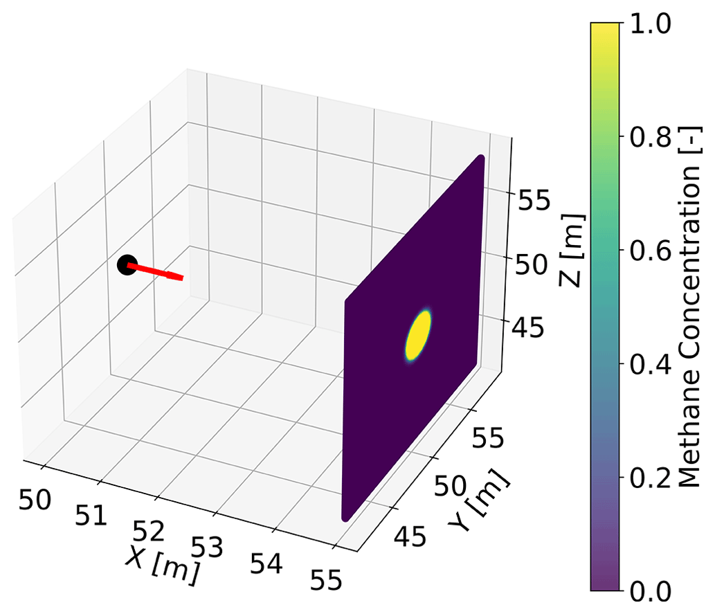
Figure 1 The 3-dimensional normalized methane concentration above the background on a curtain flight located 5 m downwind of the source (black circle). The wind velocity is shown with a red vector. The Gaussian plume is assumed to have 5° horizontal and vertical opening angles. There is a horizontal spacing of 0.09 m between the measurement points and a vertical spacing of 0.3 m vertical flight lines.

Figure 2 illustrates the concentration measurements in the Pz plane along with the calculated emission rate for the source considered in Fig. 1 for coarse and fine vertical spacing. The quality of the emission rate estimate degrades with the increasing coarseness of the flight lines in the vertical direction, resulting in a deviation of 0.229 kg h⁻¹ (4.6 % relative error) for a vertical spacing of 1 m.

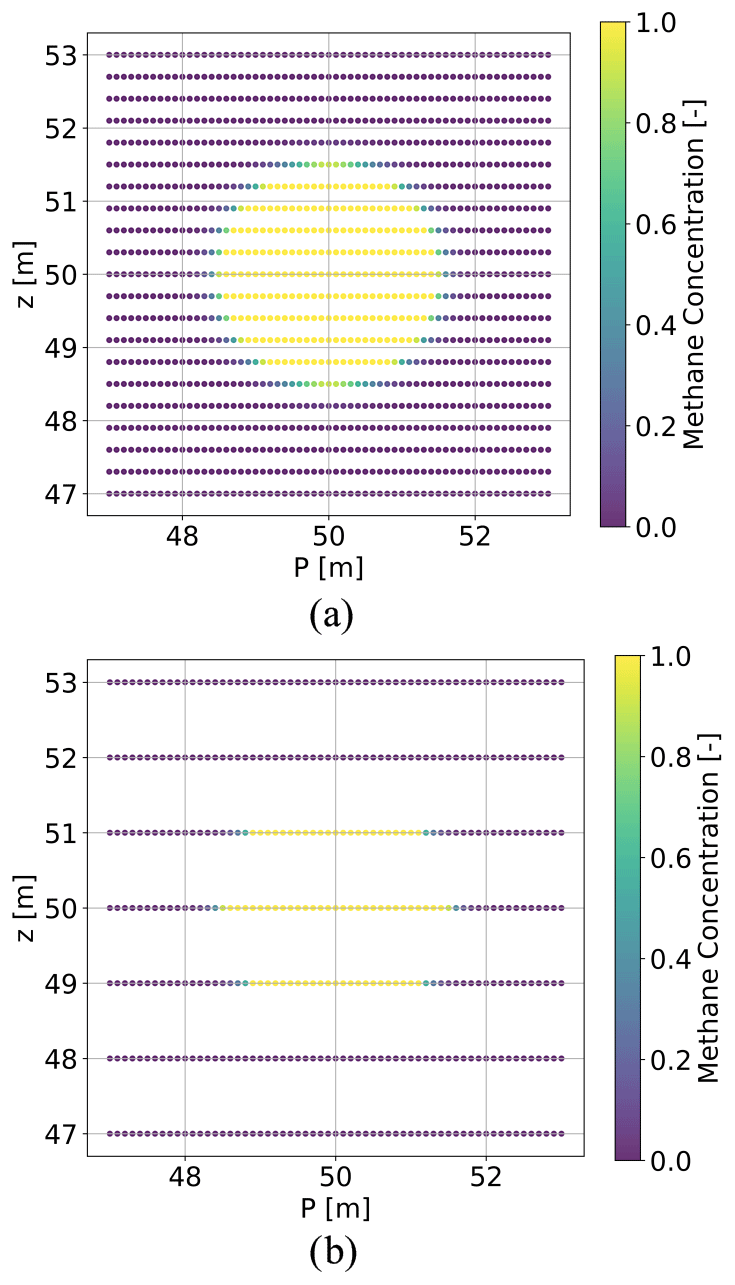
Figure 2 A 2D illustration (Pz plane) of the normalized methane concentration above the background simulated using a Gaussian plume for a 2-dimensional curtain flight 5 m downwind from the source, with a horizontal spacing of 0.09 m between the coordinates and vertical spacing of (a) 0.3 m with the calculated emission rate equaling 5 kg h⁻¹ and (b) 1.0 m with the calculated emission rate equaling 5.229 kg h⁻¹.

3.2 Horizontal and vertical spacings of the curtain drone measurements

3.2.1 Non-equidistant vertical spacing

In Sect. 3.1, the horizontal and vertical spacings between the flight coordinates are assumed to be constant. In practice, however, the assumption of equidistant spacing is easily violated. Here we assess the effect of varying spacing in the vertical direction on the emission rate error. For L number of flight lines, L random samples from a Gaussian distribution with zero mean and a standard deviation σ_l are drawn as

$$\begin{array}{}\text{(14)}& l_i\sim \mathcal{N}(\mathrm{0},{\mathit{\sigma }}_l^{\mathrm{2}}),i=\mathrm{1},\mathrm{2},\mathrm{\dots },L,\end{array}$$

where ${\mathit{\sigma }}_l^{\mathrm{2}}$ equals a percentage (ranging from 1 % to 100 %) of the vertical spacing. For a flight line i, l_i is added to the simulated vertical coordinates of the drone measurements (z). This means the drone measurements on the flight line $i,i=\mathrm{1},\mathrm{2},\mathrm{\dots },L$ are all shifted equally. For each simulation scenario (i.e., each standard deviation) 300 independent runs are considered.

Figure 3 shows the box–whisker plot for the emission rate percentage error for non-equidistant vertical spacing. There is no bias in the calculated emission rate with increasing variation in the vertical spacing, but individual measurement cases can have errors of up to almost 40 % if the standard deviation in the vertical spacing is equal to the nominal vertical spacing. Non-equidistant vertical flight lines introduce the possibility of missing the plume. Having a larger percentage of the vertical spacing as the standard deviation of the Gaussian distribution means that the non-homogeneity between the vertical flight lines becomes more pronounced. This means that one might miss the plume by a larger extent.

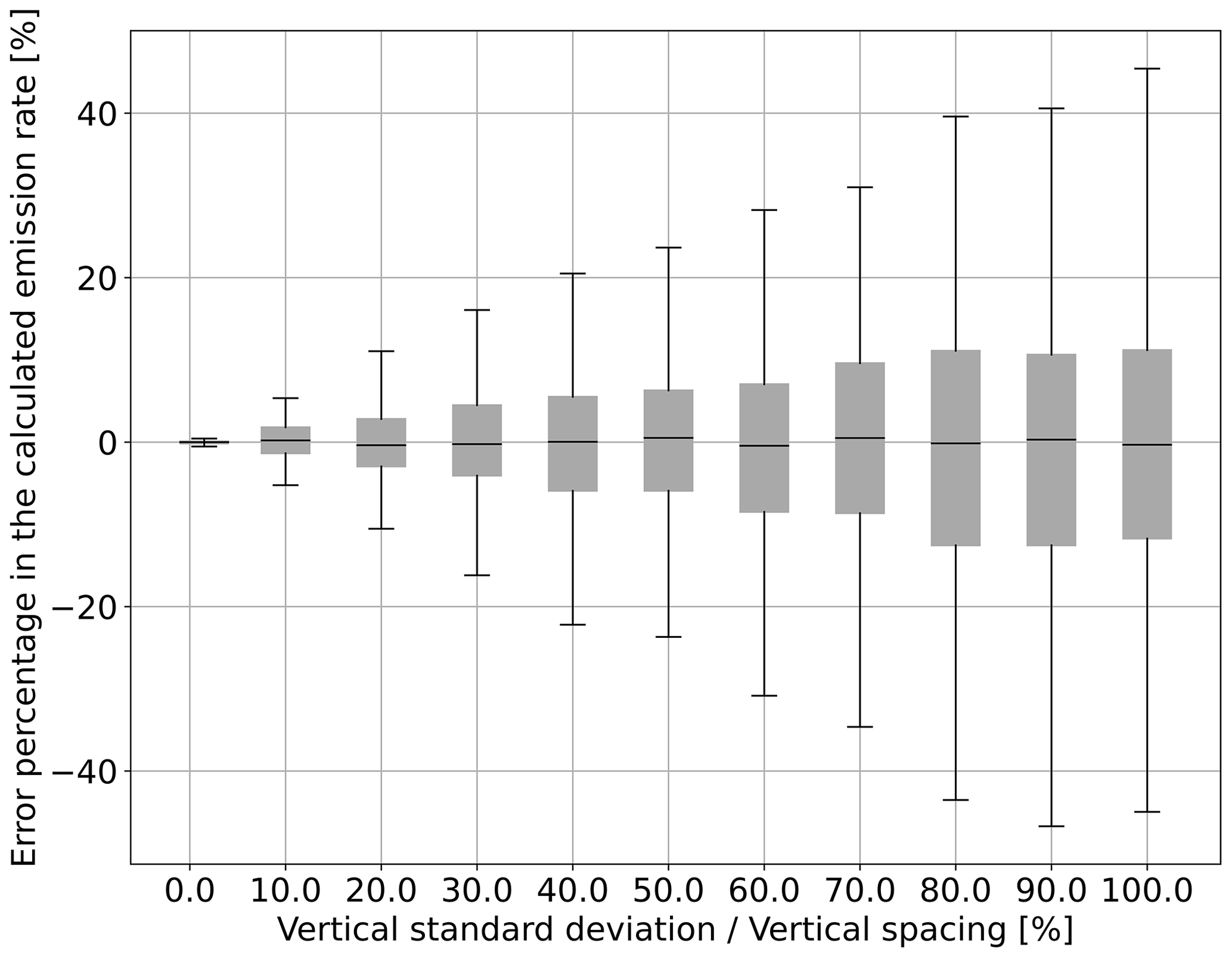
Figure 3 Box–whisker plots for the calculated emission rate error for increasing standard deviation of the vertical spacing between flight lines. Here and henceforth, the gray bars denote the 25 % (Q₁)–75 % (Q₃) quantile range; the lower and upper whiskers show the Q₁–1.5 IQR and Q₃+1.5 IQR, with IQR being the interquartile range of the values simulated.

3.2.2 Missing the plume center in relation to horizontal and vertical spacings

In Sect. 3.1, it is assumed that one flight line passes through the center of the plume in the vertical direction and a concentration point exists on this flight line corresponding to the maximum concentration of the plume on the 2-dimensional curtain. In practice, these assumptions are easily violated as the location of the source is not exactly known. Therefore, here we will assess the potential uncertainty induced by missing the maximum concentration of the plume for different horizontal and vertical spacings of the drone measurements. The resulting error is a function of the horizontal and vertical spacings as the drone is more likely to miss the highest concentration of a plume if the horizontal and/or vertical spacing is large. To assess the effect of missing the plume, for each horizontal (ΔP) and vertical (Δz) spacing of the drone measurements, 15 different shift values relative to the plume center (projected on the curtain) ranging from $-\frac{\mathrm{\Delta }P}{\mathrm{2}}$ to $+\frac{\mathrm{\Delta }P}{\mathrm{2}}$ in the horizontal direction and from $-\frac{\mathrm{\Delta }z}{\mathrm{2}}$ to $+\frac{\mathrm{\Delta }z}{\mathrm{2}}$ in the vertical direction are considered. For each shifted location, the emission rate error is calculated, i.e., 225 (15×15) instances of calculated emission rate errors. For all the locations except the one where one flight line passes the center of the plume, the maximum concentration is missed. Therefore, the emission rate is usually underestimated, and the maximum error representing the worst situation is considered for each combination of horizontal and vertical spacings.

For a plume with a known opening angle in the horizontal and vertical directions (ω_h and ω_v), the calculated emission rate remains unchanged for a varying downwind distance d if the horizontal and vertical spacings are scaled according to the opening angle of the plume. In order to have a generic representation of the maximum error for different horizontal and vertical spacings and a downwind distance d, the horizontal (ΔP) and vertical (Δz) spacings can be expressed as factors of the plume horizontal and vertical standard deviations, σ_h and σ_v in Eq. (11b), respectively, as the following dimensionless quantities:

$$\begin{array}{}\text{(15a)}& {\displaystyle }\mathrm{\Delta }{P}^{\prime }& {\displaystyle }={\displaystyle \frac{\mathrm{\Delta }P}{{\mathit{\sigma }}_{\mathrm{h}}}}={\displaystyle \frac{\mathrm{\Delta }P}{\mathrm{d}\tan {\mathit{\omega }}_{\mathrm{h}}}},\text{(15b)}& {\displaystyle }\mathrm{\Delta }{z}^{\prime }& {\displaystyle }={\displaystyle \frac{\mathrm{\Delta }z}{{\mathit{\sigma }}_{\mathrm{v}}}}={\displaystyle \frac{\mathrm{\Delta }z}{\mathrm{d}\tan {\mathit{\omega }}_z}}.\end{array}$$

Shown in Fig. 4 is the maximum error in the calculated emission rate for different dimensionless horizontal and vertical spacings for a curtain flight located 5 m downwind of a source with the emission rate $\dot{m}=\mathrm{5}$ kg h⁻¹. As seen, the estimated emission rate error decreases with higher frequency (i.e., smaller horizontal spacing) and smaller vertical spacing. It should be highlighted that even with a high-frequency drone flying with a small vertical spacing, the error will not reach zero due to the existence of other error contributors.

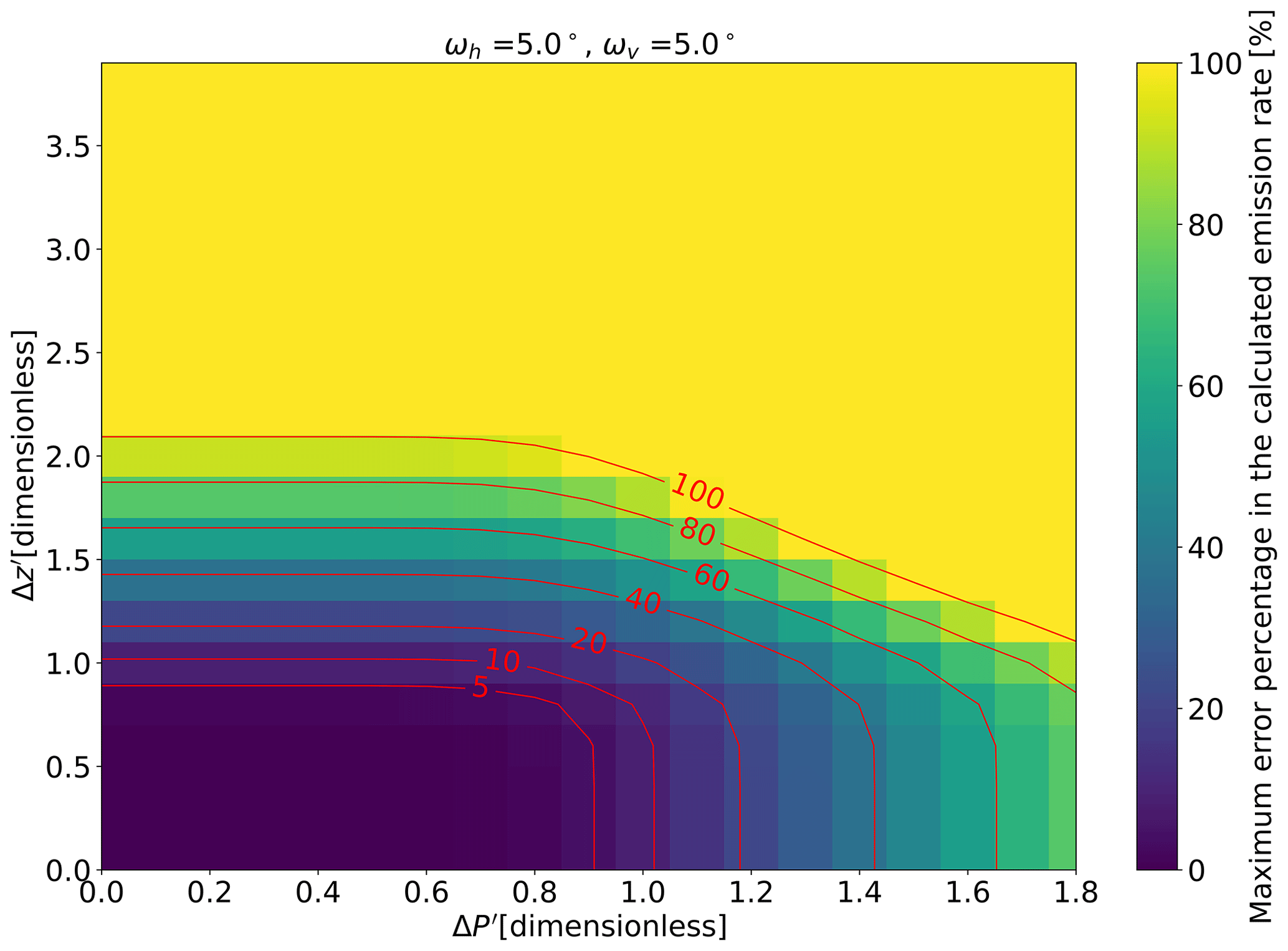
Figure 4 Maximum emission rate error in percentage (over 225 experiments corresponding to missing the plume by different percentages of the horizontal and vertical spacing) for varying dimensionless horizontal and vertical spacings. Shown with red are the error contours.

3.3 Angle between flight lines and wind direction

In the ideal situations described in Sect. 3.1, the drone flies in a direction perpendicular to the wind field. However, in real-world scenarios such a flight design might be impractical due to the existence of buildings and obstacles or safety requirements. It is thus relevant to assess how the deviation of the flight curtain from the direction perpendicular to the wind field affects the calculated the emission rate. Figure 5 shows the result as a function of the angle of the curtain with respect to the wind direction for three different values of the plume opening angle. As seen, the error is negligible for situations in which the deviation of the 2-dimensional curtain from the direction perpendicular to the wind field is less than 45°. If the flight pattern is not perfectly perpendicular to the wind direction, an error term emerges due to the effect of diffusion (see first term on the right-hand side of Eq. 4). In the mass balance equation, Eq. (5), the diffusion term is discarded and only the advection term is considered. For the non-perpendicular flight patterns, however, the term $\mathit{n}\cdot {\mathit{e}}_y\frac{\mathrm{d}c}{\mathrm{d}y}$ in Eq. (4) is not exactly equal to zero (here, e_y denotes the unit vector pointing in the y direction). For a westerly wind field, the deviation in the northern part of the plume may, to first order, be compensated by opposite deviations in the southern part of the plume, but the deviations can become considerable at large measurement angles. The actual contribution of the error from this source is proportional to the value of the diffusion coefficient K, and it leads to a slight overestimate of the mass emission rate that increases with the opening angle of the plume (usually the opening angle is proportional to K). If the flight trajectory deviates from the direction perpendicular to the wind by more than ≈70°, underestimation occurs and the magnitude of underestimation increases with the deviation angle. The main cause for this error is that part of the diverging plume will never be captured by the vertical curtain; if the opening angle is larger, a larger percentage of the plume will be missed in this way and the error thus increases.

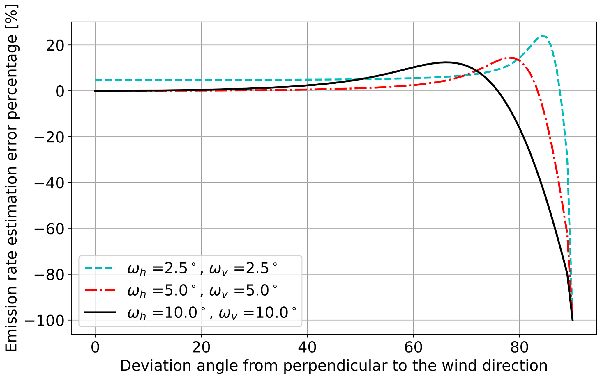
Figure 5 The emission rate error percentage as a function of deviation of the 2-dimensional curtain from the direction perpendicular to the wind velocity obtained from the simulation. Results are shown for three different opening angles of the Gaussian plume: 2.5, 5, and 10°.

3.4 Time variations in wind speed and/or wind direction

Another assumption considered in Sect. 3.1 was that the wind field is time-invariant; however, in practice this assumption is rarely true. To take this issue into account, we consider a large number of simulations in which a Gaussian plume changes randomly according to the Ornstein–Uhlenbeck process described in Sect. 2.4. The factor τ is chosen to be equal to 30 s in all simulations. Each simulation starts with a westerly wind of 5 m s⁻¹, but it gradually evolves into a fluctuating wind field with a statistical standard deviation in the wind speed and/or in the wind direction in accordance with a pre-defined factor σ_χ (see Eq. 13). For each standard deviation, 300 independent simulation runs are performed, and the results are shown for time-varying wind direction (panel a), time-varying wind speed (panel b), and their combination (panel c) in Fig. 6.

Figure 6a shows that the percentage error increases with increasing wind direction variability. The plumes do not stay in the same location during the simulation as the direction of its center-line changes according to the Ornstein–Uhlenbeck process, and this can lead to an underestimate or an overestimate of the spatial extent of plumes or other plumes being measured multiple times. In any case, the error increases as a result of increased variability in wind direction. The percentage error grows with the wind variability until the wind direction variability reaches a value of approximately 8°. For larger variations, the error does not increase much further. This can be explained from the timescale τ in the Ornstein–Uhlenbeck process that does not allow variations that are too rapid. Hence, the variations in wind direction may be larger over the entire simulation, but during the time of one single horizontal flight line, the variation seen by the drone will be similar. Note that we only model horizontal meandering of the plume; vertical meandering would have a similar effect, as long as source locations are far above the ground and measurements take place at high altitude as well.

Figure 6b shows what happens when we vary the wind speed. Our first observation is that the percentage error is generally much lower than in Fig. 6a. This can be directly explained from Eq. (10): the concentration level is inversely proportional to the wind velocity. As long as a fraction of the methane plume is captured, the product of cu⋅n in Eq. (3) will be approximately constant even if the wind is varying. The total mass balance equation will thus be unaffected. This holds for small variations in wind speed.

If there are very large variations in the wind speed (over about 50 % on average), it may happen that the random fluctuations may approach 100 % on occasion. If that is the case, the wind speed becomes close to 0 m s⁻¹ or the wind may even inverse the direction, which means that parts of the plume are missed. This effect can be seen as a spurious artifact of the simulation, but it bears some resemblance to what can happen in actual drone-based methane measurements in low-wind conditions: if the wind speed drops to zero, then it can become practically difficult to see any signal from the methane plume in the vertical curtain chosen.

Figure 6c applies to the situation with both time-varying wind speed and wind direction variability. Apparently, the dominant source of error at moderate variations is the wind direction. This is in line with the results in Fig. 6a and b, which showed markedly higher uncertainties for the wind direction variations.

Figure 6 Box–whisker plots for the calculated emission rate error for increasing standard deviation of (a) time-varying wind direction, (b) time-varying speed, and (c) time-varying wind velocity (both direction and speed at the same time). The 2-dimensional curtain is located 5 m s⁻¹ downwind from the source.

3.5 Other potential sources of error

There are other potential sources of error and uncertainty, such as the precision of the methane concentration sensor, uncertainty of GPS measurements, and the uncertainty of wind velocity in the turbulent atmospheric boundary layer between the source and the vertical measurement curtain during the entire time required to complete the data acquisition. The detailed properties of the emission source, such as the temperature of the emitted gas and its buoyancy, can also play a role in how a methane plume moves through the atmosphere. Finally, time variation in mass emission rates from sources are not considered in this paper, but they may well be a source of uncertainty in practice in site-level measurements under the OGMP2.0 framework.

4 Real-life examples

4.1 Historic controlled-release data from Scientific Aviation

Nine controlled-release experiments from Scientific Aviation were analyzed to gain a better understanding of the empirical uncertainty about the mass balance method, as well as a more detailed appreciation of the underlying assumptions that go into the computation of the methane emission rate. The experiments were carried out near the Scientific Aviation office in Boulder, Colorado, in 2019 and 2020.

Figure 7a shows the flight path of measurement “A”, done on 13 November 2019. The dots, which indicate the flight trajectory, are colored by the methane concentration measured. Figure 7b shows the altitude of the drone in the course of time during measurement A. Apparently, multiple transects of the methane plume were attempted at different altitudes. Figure 7c shows a time series of the methane concentration measurements.

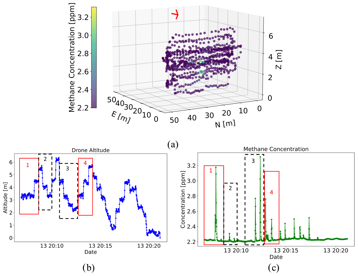
Figure 7 (a) Methane concentration data plotted against the location of measurements in a 3-dimensional space. The average wind direction is shown with the red arrow. (b) Time series of the drone altitude, with the first upward transect denoted by “1” (solid red), the first downward transect denoted by “2” (dashed black), the second downward transect denoted by “3” (solid red), and the second upward transect denoted by “4” (dashed black). (c) Concentration time series for the controlled-release data A acquired on 11 November 2019.

Although the objective was to fly a vertical curtain pattern, comparing the left graph of Fig. 7 to Fig. 1 highlights the difference between the simulated drone measurements and the actual drone measurement by a pilot. Some of the assumptions considered in Sect. 3.1 are likely violated: there is no guarantee that there will be one flight line passing the center of the plume or that the horizontal and vertical spacings between adjacent concentration will be nearly equidistant. The time series of concentration measurements and altitude indicates that there are upward (solid red) or downward (dashed black) curtains where the plume is missed. It is thus important to assess how the emission rate calculated from the mass balance method is affected by irregularities in the measurements taken by the drone.

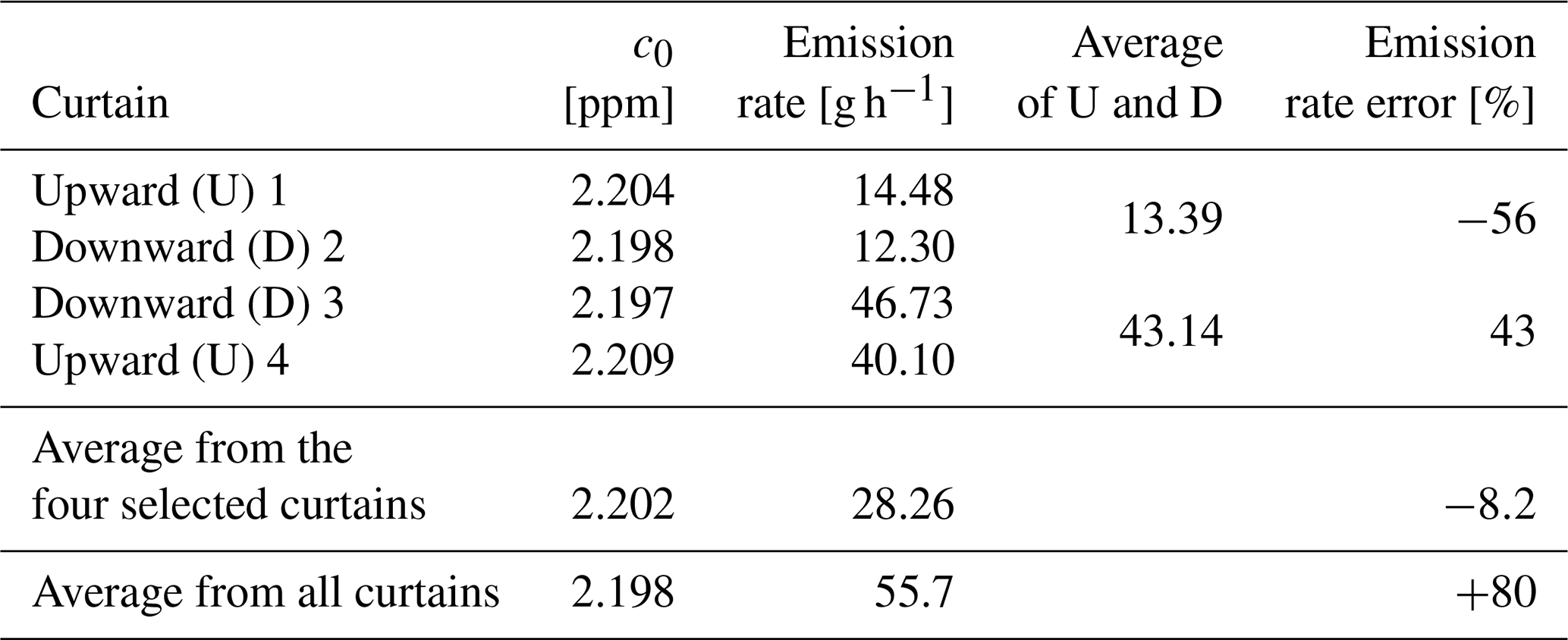
As an illustration, we will consider the data from flight A in more detail. We use a nearest-neighbor algorithm with the Euclidean distance metric to project the concentration measurements onto a vertical plane. This is only one choice for the data interpolation; other distance metrics like Chebyshev and Minkowski distances can also be used in the nearest-neighbor algorithm; other interpolation techniques such as a Gaussian smoother can also be used as an alternative to the nearest-neighbor process. Since Scientific Aviation uses the nearest neighbor for the projection of the concentration measurements on the vertical curtain plane in all their data analysis, we use the same interpolation technique to generate the results in this section. Appendix D shows that the Gaussian smoother as the interpolation technique for this data set results in similar emission rates. Using the interpolated concentration values on the plane, we can then compute the total emission rate with the mass balance method using Eq. (8), where the total mass emission rate is the average of multiple individual curtain patterns. The atmospheric background, c₀ in Eq. (6), is estimated from the 10th percentile of all the concentration measurements.

If we take into account all the concentration measurements (except those corresponding to the drone flying from the landing pad towards the curtain of interest), the average atmospheric background concentration has been determined as 2.198 ppm. The calculated emission rate using all the concentration measurements, without any postprocessing, is 55.7 g h⁻¹. This result is 80 % higher than the true release rate of 30.8 g h⁻¹.

If, on the other hand, we choose a different postprocessing method to calculate the emission rate, the results can be very different. For example, we can subdivide the flight trajectory in measurement A into two upward curtains, indicated as 1 and 4 with red rectangles in Fig. 7b, and two downward curtains, indicated as 2 and 3 with black rectangles. Shown in Fig. 8 are the 3-dimensional concentration measurements for each of these curtains. The curtains have been chosen such that they fully cover the plume. This means that three curtains at the second half of the data are discarded, resulting in the exclusion of 40 % of the data for this flight, as they do not fully cover the plume (although they have a higher concentration than the background, they only partially cover the plume), and including them in the estimate will result in an underestimation of the emission rate. It should be noted that for this postprocessing method, the atmospheric background is calculated for each curtain separately as the 10th percentile of the concentration measurements within each curtain. The uncertainty in the estimate of the background between the four curtains is 5 ppb, whereas the maximum concentration enhancements between the curtains are well above 500 ppb, implying that the uncertainty in the atmospheric background has a negligible effect on the emission rate estimate. Presented in Table 1 is the calculated atmospheric background, c₀, and emission rate for each individual upward and downward curtain using Eq. (8), along with the average emission rate from the curtains selected. The result is an emission estimate of 28.26 g h⁻¹, which is only 8.2 % lower than the true emission rate. This shows that the postprocessing method can potentially decrease the error in the calculated emission rate considerably and is a more robust alternative to using all the concentration measurements without any postprocessing.

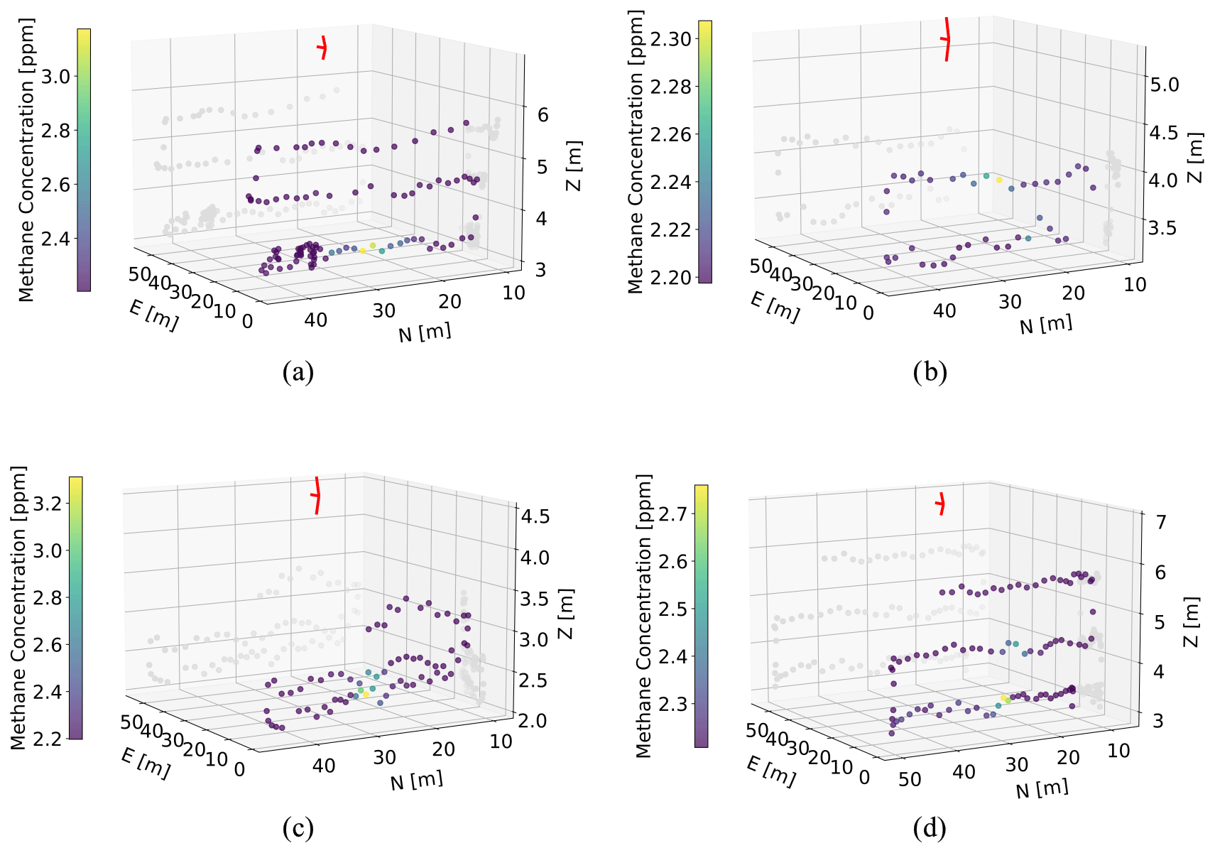
Figure 8 The 3-dimensional concentration measurements for (a) upward curtain “1”, (b) downward curtain “ 2”, (c) downward curtain “3”, and (d) upward curtain “4”. The gray dots in the figure indicate the concentration measurements projected onto the NZ and EZ plane to provide a better visualization of the 3-dimensional structure of the point cloud. The red arrow indicates the average wind direction.

Table 1 Atmospheric background c₀ and the emission rates calculated per curtain and the average emission rate between upward and downward curtains for measurement A, which was carried out on 13 November 2019. The emission rates in the table are calculated using Eq. (8). The true emission rate was 30.8 g h⁻¹.

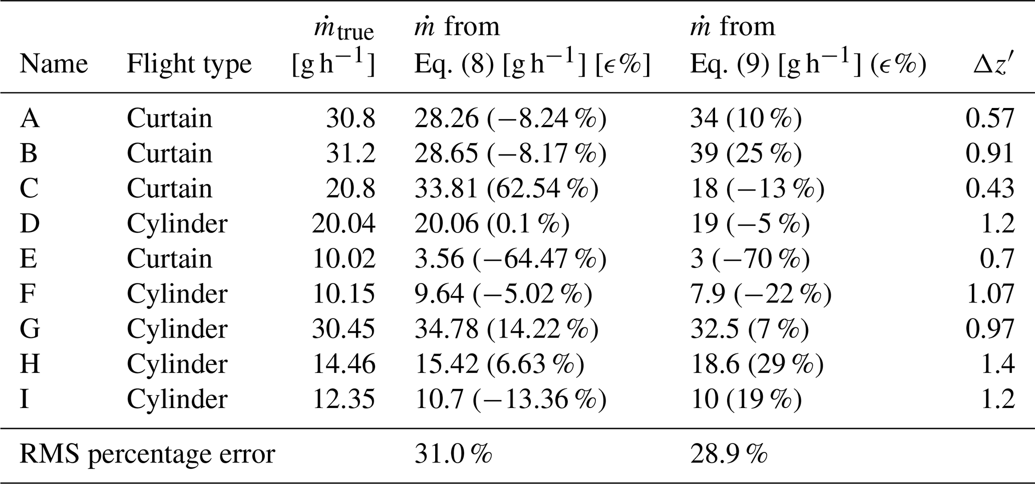
If we employ Eq. (9) for the computation of the methane emission rate, then the result is 34 g h⁻¹, which is about 10 % higher than the true answer of 30.8 g h⁻¹. The difference between the two calculation methods is due to a different interpolation methodology and postprocessing technique. Since the curtains are not equal in this case (some curtains span a larger range of altitudes than others), the latter method (using Eq. 9) gives a different result than the average of the mass emission rates computed per curtain (using Eq. 8).

Shown in Table 2 is the calculated emission rate from Eqs. (8) and (9) along with the true release rate for nine different controlled-release experiments. The last column of Table 2 shows the dimensionless vertical spacing Δz^′, computed from the flight data for each controlled-release survey using Eq. (15b). For want of detailed long-term wind data in this case, we assumed the plume opening angle ω_z to be equal to 5° in all cases. The values in the last column show that the dimensionless vertical spacing Δz^′ was smaller than 1 in most cases and never exceeded 1.4; looking back at the contour plot in Fig. 4, it is clear that the potential avoidable error due to the choice of vertical spacing was relatively low in all cases. Although, as noted earlier, this does not mean that there could not have been other sources of error, at least these are promising measurements with a small overall error if an appropriate postprocessing method is selected to process the measured concentration and wind data.

The results in Table 2 illustrate that indeed there is, in general, reasonable agreement between the calculated mass emission rates and the true methane emission rates. The root-mean square of the error percentage is 31.0 % when using Eq. (8), and it is 28.9 % when using Eq. (9). On individual cases, however, there can be a considerable difference between the two methods: see for example case C (62.54 % error versus −13 %) or case H (6.63 % error versus 29 %). There does not appear to be a systematic bias that favors one method or the other in all the cases.

A tentative conclusion from the controlled-release data is that the “best” data analytic method depends primarily on how the data were collected. For instance, Eq. (8) appears to work best in cases where the data are collected in one full curtain with sufficiently small and constant vertical and horizontal spacings and with a fairly constant wind direction during the flight. In a second or third flight, the same curtain pattern may be flown, with again enough data for a reliable mass balance calculation per flight. In that case, Eq. (8) is probably more appropriate because it uses the full mass balance method based on a direct discretization of the boundary integral (Eq. 5). We can see from Table 2 that this approach seems to work well for cylinder-shaped flight patterns in particular. On the other hand, if the data acquisition shows multiple curtains with a small number of data points per curtain (like the flight pattern from measurement A in Fig. 8, for instance), then it is wise to group the measurements together in bins per altitude in order to collect sufficient statistics to base the mass balance calculation on using Eq. (9). If Eq. (8) is used, it may be necessary to manually select useful data from less useful data – as was illustrated earlier in Table 1 for flight A.

Table 2 Calculated emission rate and the error percentage for the controlled-release experiments carried out by Scientific Aviation. Mass emission rates are computed from the data using Eqs. (8) and (9), described in Sect. 2.3. The value of the dimensionless vertical spacing Δz^′ is shown in the right-most column.

4.2 Historic measurements from SeekOps

To understand how the uncertainty in methane emission rate quantification translates into potential errors in practice, a total number of 1001 historical drone flights from SeekOps were analyzed (all the data were anonymized with regards to the geographical location and the paying customer). The data from the flights contained the position of the drone and the concentration measured at that moment in time; in addition, simultaneous data from the ground-based anemometer (at an altitude of approximately 2 m) were provided, which were extrapolated to the altitude of the drone using a predefined velocity profile from turbulent flow theory. This extrapolation itself can be a significant source of uncertainty in practice because the actual wind velocity at the position of the drone can be very different from the wind velocity measured close to the ground. Despite this caveat, we use the data from the anemometer to obtain a first estimate of the variability in the wind conditions. In summary, the following parameters were calculated from the data collected during each flight: (a) from the anemometer data – the wind average speed, wind standard deviation in north–south and east–west directions; (b) from the flight pattern – the average horizontal and vertical spacing in methane concentration measurements, as well as standard deviations of these quantities; and (c) from site layout – the downward distance from the source, estimated from the source location in an equipment area. In order to allow the uncertainty analysis as explained in Sect. 3, the raw wind data need to be converted into an absolute wind speed and their root-mean-square fluctuation, as well as a plume opening angle. The conversion process is described in the appendix.

With these parameters calculated, the potential errors were calculated for each of the 1001 historic flights by SeekOps. Based on the available information, the errors in the emission rate calculation due to the following sources are calculated for each flight: (a) not passing the center of the plume due to large vertical spacing between the flight lines, (b) non-equidistant vertical spacing, (c) time-varying wind speed, and (d) time-varying wind direction.

We will report the potential errors due to these parameters for flights in four categories, based on the plume opening angle at the time of measurement. The vertical plume opening angle in all 1001 flights analyzed covers the full range of angles from 0 to 90°. For visualization purposes, we will report the potential errors in four groups of the plume opening angles: between 0 and 22.5° (with an average opening angle of 10.7° for measurements with a plume opening angle in this category), between 21.4 and 45° (with an average of 30.5°), between 45 and 67.5° (with an average of 50.8°), and between 67.5 and 90° (with an average of 71.1°).

Not passing the center of the plume

The results for the effect of non-zero horizontal and vertical spacings in the methane concentration measurements are shown in Fig. 9. Figure 9a shows the results for the category of flights where the plume opening angle was relatively narrow. Color shades from blue to yellow indicate the increase in the errors in the calculated emission rate. The dimensionless horizontal (ΔP^′) and vertical (Δz^′) spacings are determined from the flight data provided by SeekOps; these coordinates are then plotted as orange crosses onto the contour plot that was determined for a plume with an opening angle of 10.7°. Most orange crosses are located close to the origin of the graph. This area corresponds to low potential errors due to the choices of dimensionless spacings. There are also flights, however, where the dimensionless spacing was larger than 1 (in horizontal and/or in vertical direction), and for those cases the errors become potentially very large: more than 100 % of the measured value. The reason why there is a significant number of data points in this region may actually be due to unexpectedly coherent wind situations: if the wind is steady and turbulent fluctuations are low, then the plume opening angle is small, and the dimensionless horizontal and vertical spacings can become large since the opening angle is in the denominator of Eq. (15b) (through Eq. 11b). There is thus the risk that the plume passes through the flight lines, meaning that the drone misses the plume altogether.

The results for the wide plume opening angles are shown in the other panels of Fig. 9. In these cases, we see that most data points from SeekOps flights are located near the origin in regions where the expected error is relatively low.

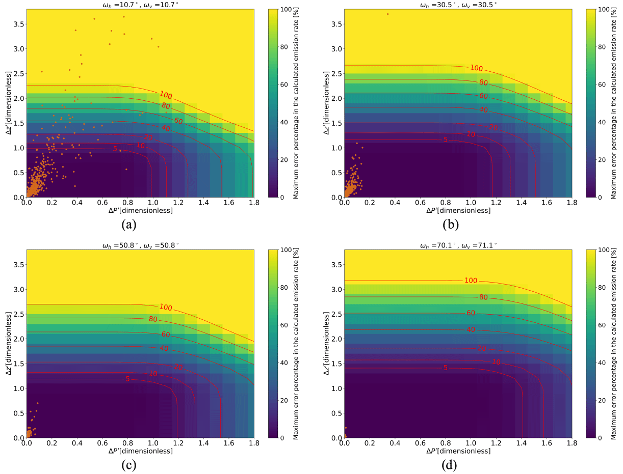
Figure 9 Contours indicate maximum calculated emission rate error (over 225 calculations corresponding to missing the plume by different percentages of the horizontal and vertical spacings) for varying dimensionless horizontal and vertical spacings for four different groups of plume opening angles: (a) plume opening angle of 10.7°, (b) plume opening angle of 30.5°, (c) plume opening angle of 50.8°, and (d) plume opening angle of 71.1°. The orange dots indicate the horizontal and vertical spacings for four different groups of plume opening angles: (a) between 0 and 22.5°, (b) between 21.4 and 45°, (c) between 45 and 67.5°, and (d) between 67.5 and 90°. Shown with red are the error contours.

Non-equidistant vertical spacing

Now we analyze the errors that can potentially occur due to the standard deviation of vertical spacings. The result is shown in Fig. 10, for each of the four categories of plume opening angles. The box–whisker plot is generated from the numerical simulations described in Sect. 3 using the average horizontal and vertical spacings, vertical opening angles, and downwind distance over 300 runs. For each run, the flight coordinates are generated by varying the flight lines randomly using a Gaussian distribution. The green bars are a histogram of the incidence rate in the 1001 flights of the ratio between the vertical standard deviation and the vertical spacing. Figure 10a shows the results for the category of flights where the plume opening angle was relatively narrow. The results for the wide plume opening angles are shown in the other graphs of Fig. 10. For most flights, the variation in the vertical spacing is less than 10 % of the vertical spacing. Therefore, this effect is not expected to be a major source of error or uncertainty in the measurement.

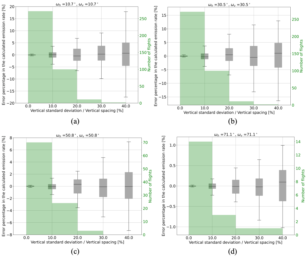
Figure 10 Theoretical box–whisker plots due to non-equidistant vertical spacing for four different groups of plume opening angles: (a) plume opening angle of 10.7°, (b) plume opening angle of 30.5°, (c) plume opening angle of 50.8°, and (d) plume opening angle of 71.1°. The green bars show the histogram of the actual flight data as a function of the vertical standard deviation divided by the vertical spacing for four different groups of plume opening angles: (a) between 0 and 22.5°, (b) between 21.4 and 45°, (c) between 45 and 67.5°, and (d) between 67.5 and 90°.

Time variation in wind speed and/or wind direction

We will now look at the errors that can potentially occur due to time-varying wind direction and wind speed, shown in Figs. 11 and 12, respectively. For each flight, the location on the horizonal axis is calculated using the wind speed and wind direction, as well as their corresponding standard deviation. The errors bars are calculated from the numerical simulations described in Sect. 3 from the average over 300 independent runs per flight. For each run, the wind speed and wind directions are generated from the Ornstein–Uhlenbeck process. The box–whisker plot is generated using the average wind speed, wind direction, and their corresponding variations and vertical opening angles.

Figure 11a shows the results for time-varying wind directions for the category of flights where the plume opening angle was relatively narrow. The results for the wide plume opening angles are shown in the other graphs of Fig. 11. Most flights have a wind direction variability of less than 40°, and for increasing wind direction variability, the absolute error increases linearly. It can also be seen across all graphs in Fig. 11 that the higher opening angles typically correspond to higher variation in the wind direction (see, e.g., the horizontal axes in Fig. 11c and d).

Figure 11 Potential box–whisker plots to time-varying wind direction. (a) Plume opening angle of 10.7°, (b) plume opening angle of 30.5°, (c) plume opening angle of 50.8°, and (d) plume opening angle of 71.1°. The green bars show the histogram of the actual flight data as a function of the vertical standard deviation divided by the vertical spacing for four different groups of plume opening angles: (a) between 0 and 22.5°, (b) between 21.4 and 45°, (c) between 45 and 67.5°, and (d) between 67.5 and 90°.

Figure 12a shows the results for time-varying wind speed and for the category of flights where the plume opening angle was relatively narrow. As the plume opening angle gets wider and the variation in the wind speed increases, the error percentage in the calculated emission rate increases.

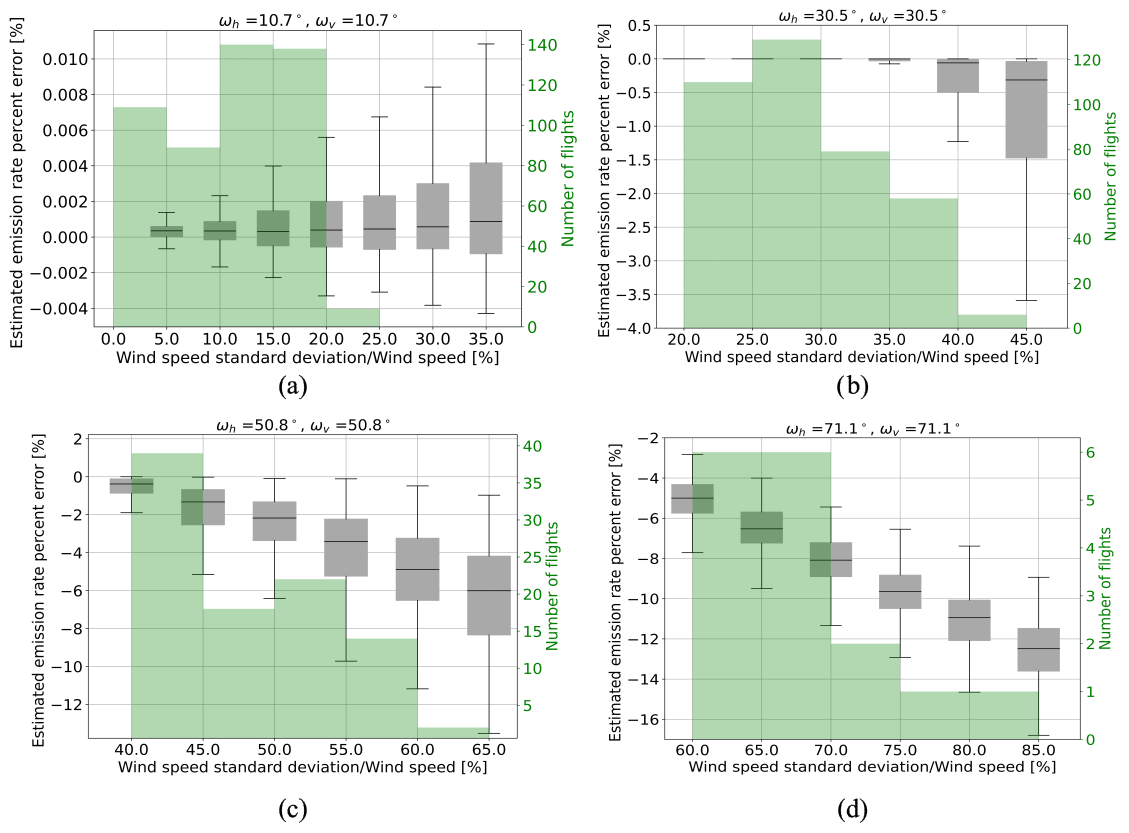
Figure 12 Potential box–whisker plots due to time-varying wind speed. (a) Plume opening angle of 10.7°, (b) plume opening angle of 30.5°, (c) plume opening angle of 50.8°, and (d) plume opening angle of 71.1°. The green bars show the histogram of the actual flight data as a function of the vertical standard deviation divided by the vertical spacing for four different groups of plume opening angles: (a) between 0 and 22.5°, (b) between 21.4 and 45°, (c) between 45 and 67.5°, and (d) between 67.5 and 90°.

By means of summary, Fig. 13 shows the cumulative statistics over all 1001 flights with regards to the theoretical error percentage in the emission rate for each of the different sources of errors discussed above. Not passing the center of the plume has the largest contribution, as was already observed in Fig. 9a. About 55 % of the flights could have an emission rate percentage theoretical error of more than 10 % because of missing the center of the plume. The other sources of error usually have a smaller impact. For instance, all the measurements have less than a 10 % theoretical error due to non-equidistant vertical flight lines. For the contribution of the time-varying wind speed, around 55 % of the flights have less than a 10 % error in the calculated emission rate; the effect of time-varying wind direction is expected to be larger than 10 % only in 20 % of the cases. Around 70 % of the flights have the emission rate error of less than 50 % due to not passing the center of the plume. Between 97 % and 100 % of the flights have less than a 50 % theoretical error in the calculated emission rate due to time-varying wind direction and speed and non-equidistant vertical flight lines.

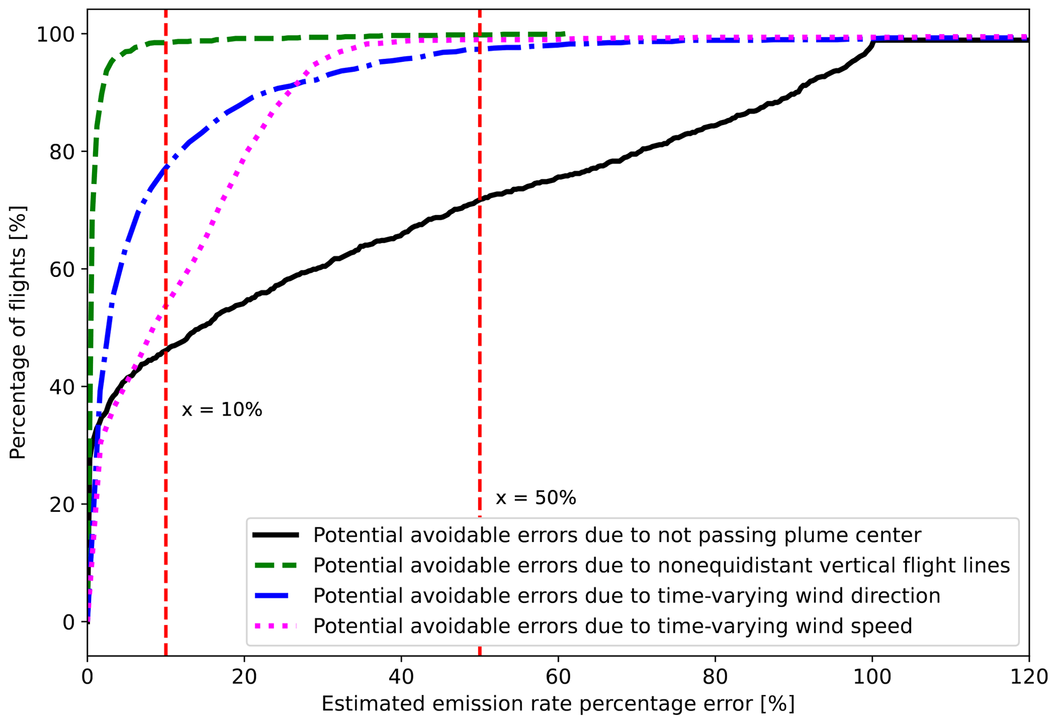
Figure 13 Cumulative distribution of flights (totaling 1001) as a function of theoretically calculated maximum error for potential avoidable error percentage due to not passing the plume center (solid black), non-equidistant vertical flight lines (dashed green), time-varying wind directions (dotted–dashed blue), and time-varying wind speed (dotted pink). Vertical dashed red lines indicate 10 % and 50 % error in the estimated emission rate.

5 Discussion

The theoretical framework presented above allows for a post hoc analysis of methane emission quantification surveys. With this, a number of potential errors and uncertainties in the measurements can be identified.

The analysis of historic flight data from Scientific Aviation in controlled-release experiments, reported in Sect. 4.1, shows that there can be a wide range of outcomes in the mass balance method for different curtain flights – even during the same controlled-release event. For the best result, the data analysis procedure must be adapted to the measurements taken.

The theoretical analysis can also be used to evaluate the quality of a historical data set of a large number of surveys. From the analysis reported in Sect. 4.2, it seems that the largest risk of uncertainty is caused by a vertical spacing of the flight lines that is too large in combination with a relatively short downwind distance from the source. The uncertainty is highest in cases when the wind field is steady and the plume opening angle is small – contradicting some “conventional wisdom” in the industry that the uncertainty is always lowest when the wind field is steady. What we find is that this assumption is only true if the measurements are taken at a sufficient distance downwind of a source with a sufficiently small vertical spacing between flight lines.

In addition to this risk of missing the methane plume in the case of steady winds, it becomes also clear from our analysis (Fig. 11c and d, in particular) that large fluctuations in the wind direction can result in a significant error. Such a situation typically occurs when the atmosphere is unstable or when the average wind speed is very low. In these cases, the fast diffusion of the methane plume can easily result in parts of the plume being missed; indeed, Fig. 11c and d show that the methane emission is usually underestimated by the mass balance method in these cases.

Our observations can also provide guidelines for future campaigns. The two main recommendations based on the present work are as follows. (a) For each individual quantification survey, fly multiple curtain patterns and choose the appropriate data analysis method to avoid excessive influence of unrepresentative data (outliers) on the result. (b) Take measurements with a sufficiently small vertical spacing and at a sufficiently large distance downwind of the source for the wind conditions on the day. In particular, the dimensionless horizontal and vertical spacings ΔP^′ and Δz^′ have to be smaller than 1 for the best result (see Eq. 15b for the full expression).

On the other hand, however, the downwind distance should not be so large that methane plumes from the facility of interest are missed. Measurements very far downwind are also unfavorable because of the lower methane concentrations expected, which will lead to a lower signal-to-noise ratio. We recommend to use values of ΔP^′ and Δz^′ between 0.1 and 1.0 in practical applications. To make this guideline more practical, if we assume that most opening angles are larger than 5°, which is the case in about 98 % of the 1001 onshore drone flights considered in this paper, then the guidance is that the vertical and horizontal spacings have to be smaller than $\mathrm{1}/\mathrm{10}$ of the downwind distance to the source; in offshore measurements, this guidance may have to be adapted to address the different atmospheric stability over open water.

As a final reflection, we would like to emphasize that we have not focused in this paper on the measurement uncertainty of the sensors. This means that we do not account for possible deviations due to finite precision in the methane concentration measurements, nor do we assume any error in the wind measurement. In addition, our analyses are based on the assumption that the wind vector at the position of the drone is determined perfectly. In reality, of course, this is never the case, and there are various methods deployed by different service providers to measure the wind. We only observe here that any error in the wind measurement is likely to propagate in the computations in the mass balance method as per Eq. (6). It is not wise to assume that any error in wind measurement will somehow be compensated for by other errors. Notwithstanding other sources of error, we believe that this paper provides some guidelines to minimize avoidable errors that can result from choices in the data acquisition process and in the methodology used for postprocessing.

6 Conclusions

Site-level measurements of methane emissions are often used by operators for reconciliation with bottom-up emission inventories with the aim of improving accuracy, thoroughness, and confidence in reported methane emissions. In that context it is of critical importance to minimize measurement errors and to understand the associated uncertainty. This paper describes a systematic analysis of potential errors in methane emission quantification surveys using the mass balance method for parameters related to the acquisition of concentration data and the method of postprocessing. The analysis is applied to a quadcopter drone with a high-precision methane sensor flying in a vertical curtain pattern; the total mass emission rate can then be computed post hoc from the measured methane concentration data and simultaneously measured wind data. We find that the most important source of potential error can be expressed as a dimensionless number with the spatial resolution of the methane concentration measurements and the downwind distance from the main emission sources. The potential error is largest (and, indeed, can be as high as 100 %) in situations where the wind speed is steady and the methane plume has a coherent shape – contradicting the intuition of some operators in the industry.

What has been learned from our theoretical error analysis has been applied to a number of historical measurements in a controlled-release setting. We show how what is learned about the main sources of error can be used to eliminate potential errors during the postprocessing of flight data; we show that the reported results can be very close to the actual methane emission rates if the appropriate data analysis method is selected. Second, we have evaluated an aggregated data set of 1001 historical drone flights. Our analysis shows that the potential errors in the mass balance method can be of the order of 100 % on occasions, even though the theoretical error from the identified error sources was relatively small in the majority of the flights considered.

The Discussion section provides some guidelines on how to avoid or minimize potential errors in drone measurements for methane emission quantification. The two main recommendations are (1) to fly multiple curtain patterns in each individual survey in combination with an appropriate data analysis method to avoid excessive influence of unrepresentative data (outliers) on the result and (2) to take measurements with a sufficiently small vertical spacing and at a sufficiently large distance downstream of the source for the wind conditions on the day, with the dimensionless horizontal and vertical spacings ΔP^′ and Δz^′ both smaller than 1. There is an optimum though: downwind distance should not be so large that methane plumes from the facility of interest are missed, and measurements very far downwind are also unfavorable because of the lower signal-to-noise ratio. It appears to us that values of ΔP^′ and Δz^′ between 0.1 and 1.0 are optimal.

Appendix A: Sensor description

The main paper describes two historic data sets of methane emission measurements: one set from Scientific Aviation and one set from SeekOps. Both data sets contain concentration measurements taken by a high-precision methane sensor mounted on a quadcopter drone. The present section presents background on the type of sensor that has been used in these deployments. The text below is applicable to the sensor developed and used by SeekOps; Scientific Aviation use a commercial off-the-shelf sensor that has similar characteristics.

The SeekIR sensor used by SeekOps is the culmination of years of research and commercial development, initially at the United States National Aeronautics and Space Administration (NASA) Jet Propulsion Laboratory (JPL). The technology was originally developed for the Mars Curiosity Rover to look for evidence of microbial life and was thus developed to be extremely sensitive to methane enhancements above background levels (Webster, 2005). In 2017, the technology was spun out of JPL and commercialized for the broader energy industry, including traditional oil and gas, biogas/landfill gas, and renewable natural gas (NASA, 2019). It was subsequently validated by blind controlled-release tests performed at the Methane Emissions Technology Evaluation Center (METEC) in Colorado, where the sensor was described as being the most successful in detecting and quantifying leaks, with no false positive and no false negatives (Ravikumar et al., 2019).

The sensor operates on the principle of absorption spectroscopy, using a tunable diode laser (TDL) within an open cavity bounded by two mirrors that give a suitable path length for the laser to ensure high sensitivity to the absorption in the presence of methane molecules. This physical process is described by the Beer–Lambert law, which describes how the spectral intensity measured at a specific wavelength after passing through a sample can be used to characterize physical parameters based on an initial spectral intensity and absorption path length (Hanson et al., 2016). When parameters such as pressure, temperature, wavelength, and path length are measured or known, the concentration of the species of interest can be calculated by this change in spectral intensity. In the system described, the initial spectral intensity source is a TDL and the sensor measuring the change in spectral intensity is a photo-voltaic detector sensitive at the same spectral region as the laser light source. The detector measures the remaining photons that were not absorbed by the methane molecule(s) as part of the absorption process. A spectroscopic approach, wavelength modulation spectroscopy (WMS), is further employed by modulating the laser intensity and wavelength at a known frequency. WMS ensures the optimal signal-to-noise ratio (SNR) and a “calibration-free” method of laser diagnostics, allowing for calibration factors that persist for the life of the instrument that are determined at the time of manufacture. With appropriate filters for elevated frequencies, the detected response can be demodulated to determine the concentration of methane that has been sampled within the open cavity (Fig. A1).

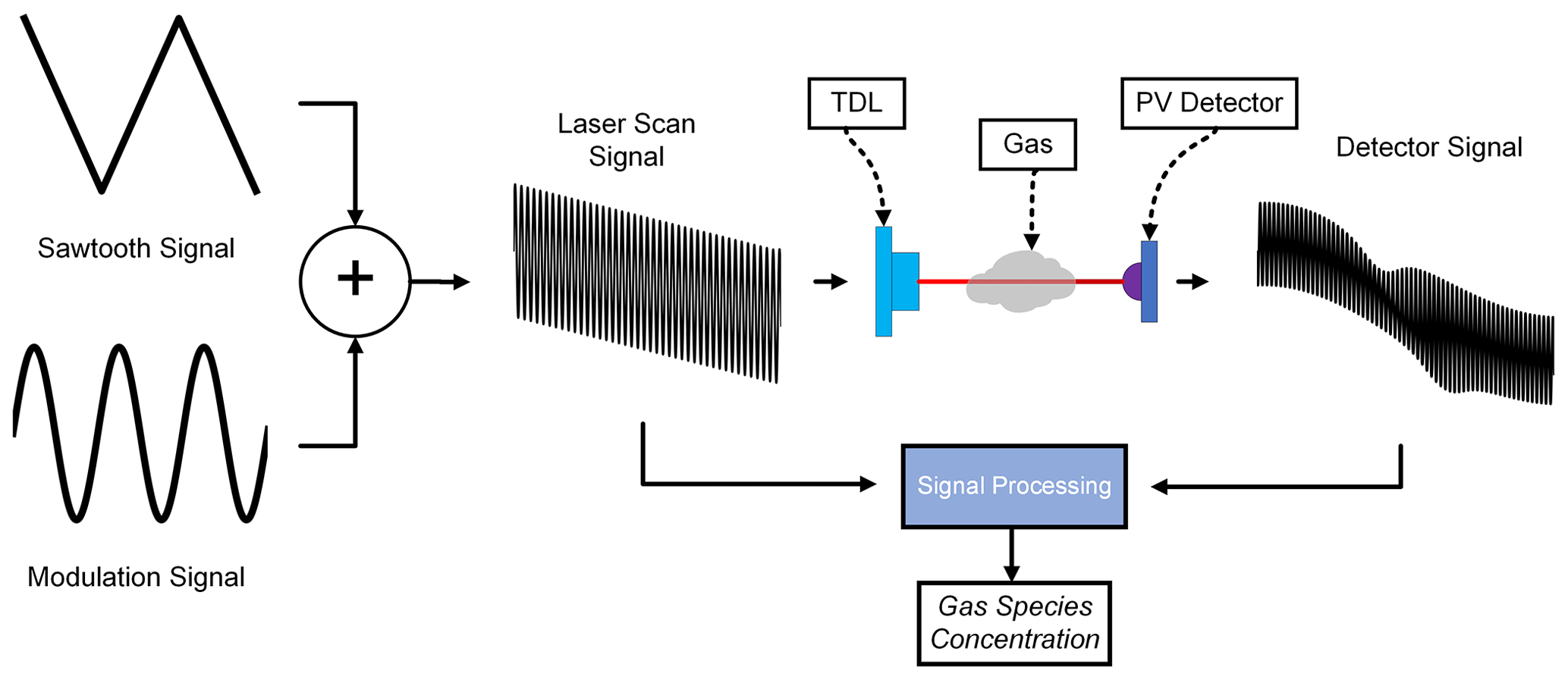
Figure A1 Simplified drawing of the implementation of wavelength modulation spectroscopy (WMS) using a tunable diode laser (TDL) for gas sample diagnostics.

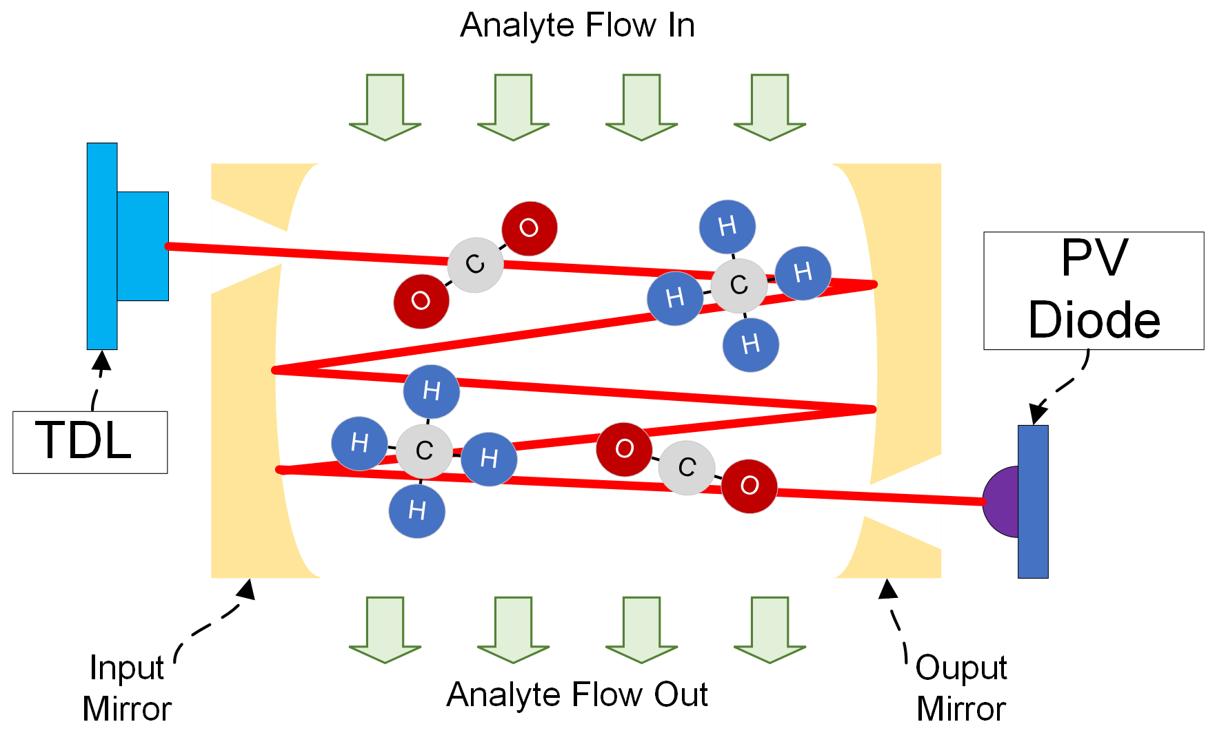
Figure A2 Drawing of the sensor operating principle of laser absorption spectrometry to determine methane concentration.

The SeekOps instrument used in this study additionally utilizes a multi-pass optical cell design, known as a Herriott cell, that increases the laser path length, further increasing its sensitivity to changes in concentration, temperature, or pressure, depicted in Fig. A2. The Herriott cell design is comprised of two concave mirrors with a high reflectivity and matched to reflect the proper wavelength of light, allowing the beam to bounce multiple times inside the cavity to help to increase the SNR and further reduce measurement uncertainty.

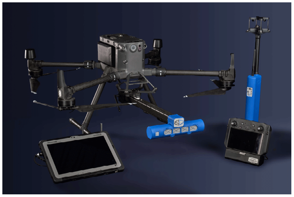
Figure A3 Methane sensor showing location of integrated GPS and lidar attached to the quadcopter drone.

Finally, great efforts have been taken to make the optical sensor robust for operations in the oil and gas sector. To this end, the sensor is mounted in a strong housing that has undergone strenuous shock and vibration testing, indicative of its operational environment when deployed on a quadcopter drone and transported to and from a facility of interest. Modern drones have multiple anti-collision sensors that can enable the sensor to be flown as close as necessary to the equipment without compromising any ongoing operations.

A picture of the SeekOps sensor is shown in Fig. A3. The sensor is mounted on an approximately 1 m long extended steel branch attached to the drone, which makes the sensor easily accessible in the case of maintenance requirements. Data acquisition takes place with the branch pointing into the wind, which allows the collection of pristine samples of air, uncontaminated by any prop wash (i.e., the airflow generated by the drone's own propellers). Methane concentration data from the sensor are streamed and displayed in real time to a ground control system (GCS). This allows for on-demand viewing of plume methane enhancements by the drone pilot so that dynamic adjustments to the survey geometry, like the horizontal and vertical spacing between concentration measurements, can be made if needed.

Appendix B: Cylindrical flight pattern

In this section, the results from the simulation of a drone flying in a cylindrical pattern are presented – similar to Sect. 3 for 2-dimensional curtain flight path. We simulated the drone flight for different scenarios with the objective of assessing the importance of various sources of uncertainty including the following:

• the position of the emission source relative to the center of the cylindrical flight paths

• the existence of multiple sources within the cylinder

• horizontal and vertical spacing in the methane concentration measurements.

Again, it is assumed that the concentration field is stationary during the time of the measurements. This can relate to a constant Gaussian plume traveling horizontally in a time-averaged horizontal wind field whose speed can vary as a function of the vertical coordinate.

B1 Ideal case

The ideal simulation case is considered in the following, similar to the ideal case considered for the 2-dimensional curtain flight (Sect. 3.1):

• constant wind field with westerly wind at a speed of 5 m s⁻¹

• one circular flight path passing through the center of the plume

• equidistant drone measurements in the horizontal and vertical directions

• no measurement error in simulated concentration, wind field, and drone measurement locations.

The radius of the cylinder, opening angles, and wind field are chosen such that they reflect a situation encountered in practice. The source with the emission rate 5 kg h⁻¹ is considered. The cylindrical flight pattern is often used for offshore applications where the horizontal and vertical opening angles of the plume are smaller than those encountered in onshore applications, and thus the opening angle of 2.5° is chosen as a realistic value for the “ideal case” (base case). Figure B1 shows the 3-dimensional concentration plot due to this source on a cylinder with a radius of 10 m.

Note that this radius is much smaller than the ≈ 300 m that Flylogix/SeekOps normally uses in surveys of offshore platforms. This should not affect the main results because the radius will appear as the length scale when considering the spacing. With a radius of 10 m, it is reasonable to assume that the methane plume is stable, as the methane in the plume only takes a few seconds to go from source to sensor. At longer distances of ≈ 300 m, the transit time is of the order of ≈ 1 min and the wind direction can vary considerably during that time.

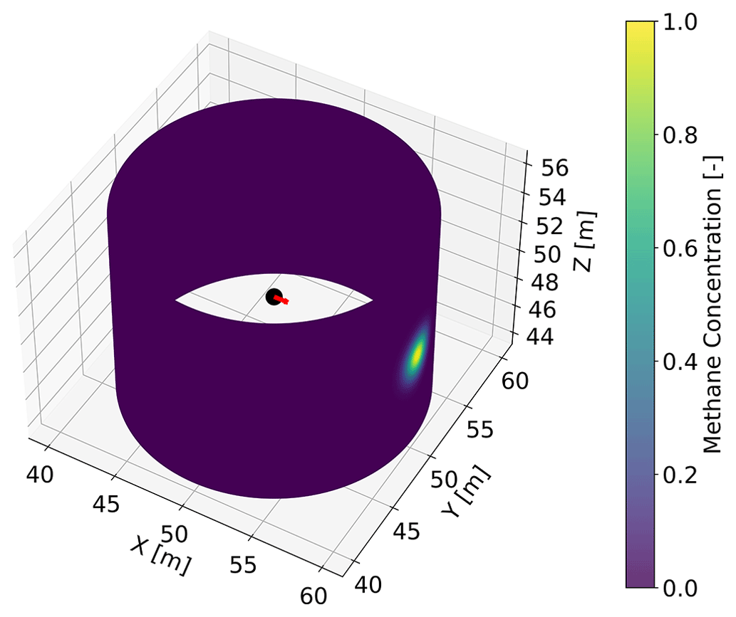
Figure B1 The 3-dimensional normalized methane concentration above the background on a cylinder with a radius of 10 m for a source located at the center of the cylinder (shown by black). The wind velocity is shown with a red vector. The Gaussian plume is assumed to have 5° horizontal and vertical opening angles. There is an angular spacing of 0.5° between the measurement points and a vertical spacing of 0.3 m.

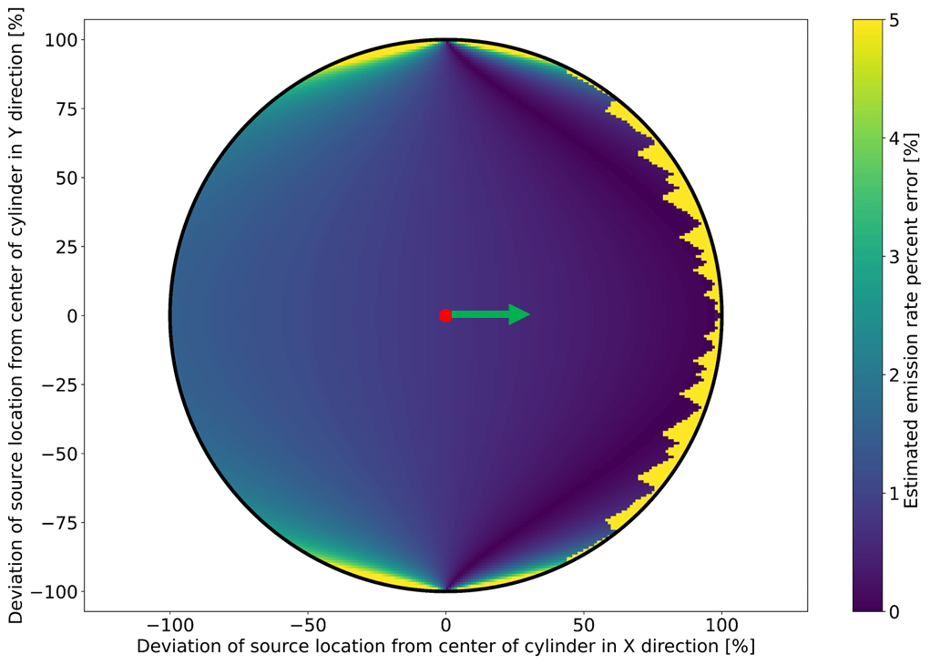
Figure B2 Calculated emission rate error percentage for shifted source in X and Y directions from the center of the cylinder as a percentage of the cylinder’s radius. The wind direction is shown with the green vector, and the center is indicated by the red circle.

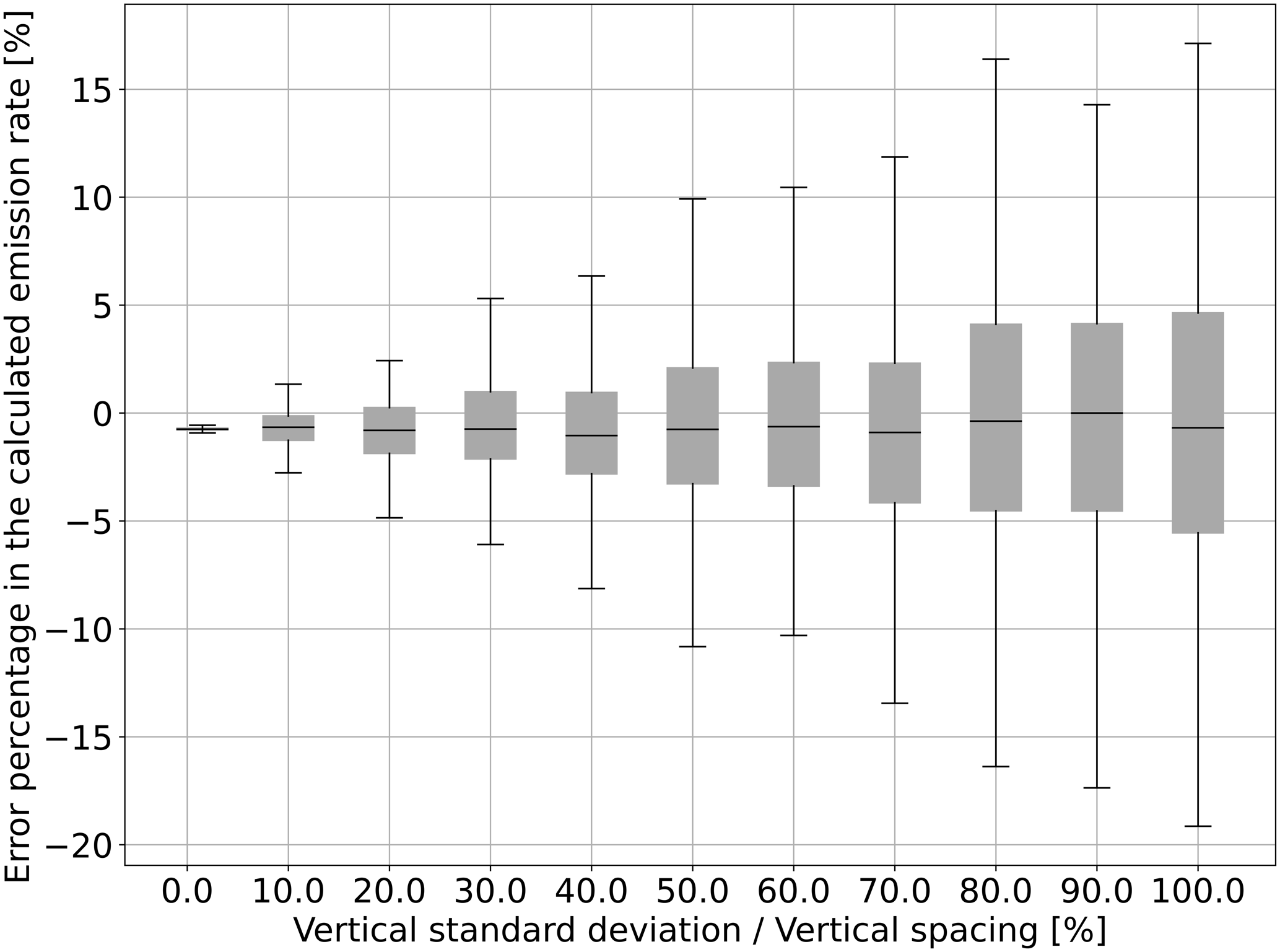
Figure B3 Box–whisker plot for the calculated emission rate percentage error for non-equidistant vertical spacing between the flight coordinates for the cylindrical flight paths.

B2 The importance of turbulent diffusion on mass emission calculation

For a cylindrical flight pattern, the true emission rate cannot be exactly retrieved. In Fig. B1, there is an error of 0.006 kg h⁻¹ (equal to a percentage of 0.12 %) even for a very fine spacing in the horizontal and vertical directions. This error does not exist for the 2-dimensional curtain situation as the true emission rate is retrieved from the mass balance equation. The emerged error term is due to the effect of diffusion (see the third term on the right-hand side of Eq. 4). If the flight path is cylindrical, the direction of the unit vector n varies along the flight path, and the contribution of n⋅∇c does not vanish along the integral. Since this term is not normally included in the mass balance equation, Eq. (6), this results in an underestimate as n⋅∇c is typically larger than 0 in the case where a source is located in the center of the cylinder. This error cannot be eliminated, even in the limit of perfectly accurate vertical and horizontal measurements; to first order, the error is proportional to the diffusion coefficient K.

B3 Position of the emission source relative to the center of the cylinder

In Sect. B1, we assumed that the source is located at the center of the cylinder; however, in practice this might not hold. It is thus beneficial to assess the impact of such an assumption on the calculated emission rate. Shown in Fig. B2 is the error percentage for varying shifts in the source from the center as a percentage of the radius of the cylinder. The wind direction is also shown with a green vector. For the situation where the source gets very close to the cylinder on the right-hand side, the term $\frac{\mathrm{d}c}{\mathrm{d}y}$ increases (as the concentration increases). One should bear in mind that the neglect of diffusion for the cylindrical flight pattern typically results in a small contribution to the error compared to the other sources considered.

Figure B2 can also be used to calculate the total error in the calculated emission rate in the case of there being multiple sources within the cylinder. We will illustrate this with an example: assume two sources A and B with true emission rates of ${\dot{m}}_A$ and ${\dot{m}}_B$, respectively. The calculated emission rate error percentage for each source, referred to as ϵ_A and ϵ_B, can be obtained from Fig. B2 using their position relative to the center of the cylinder as a percentage of the radius of the cylinder. Using these calculated emission rates, the total error in the situation where multiple sources exist within the cylinder can be obtained as ${\mathit{ϵ}}_{A+B}=\frac{{\mathit{ϵ}}_A{\dot{m}}_A+{\mathit{ϵ}}_B{\dot{m}}_B}{{\dot{m}}_A+{\dot{m}}_B}$.

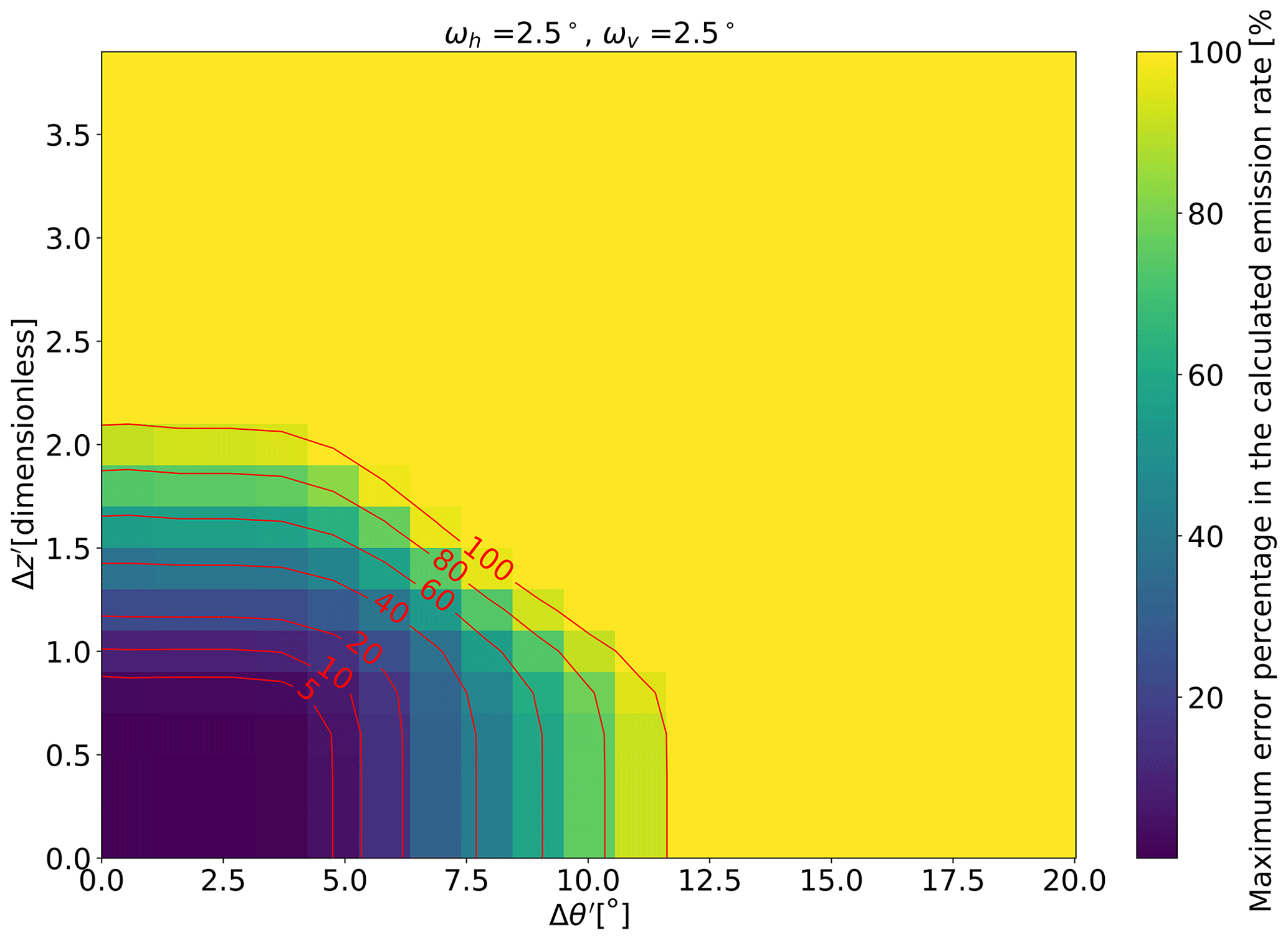
Figure B4 Maximum calculated emission estimate error for varying factors of horizontal and vertical spacings expressed as degrees and a dimensionless parameter for a plume with a vertical and horizontal turbulence of 2.5°. For each horizontal and vertical spacing, the maximum value over 225 calculations corresponding to different locations of the flight lines relative to the source is shown. Shown with red are the error contours.

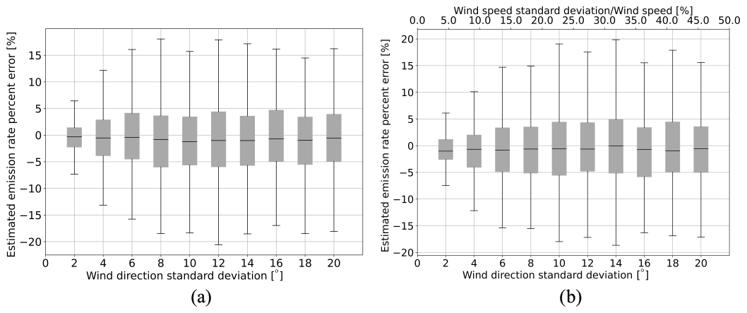
Figure B5 Box–whisker plot for the calculated emission rate error for increasing standard deviation of (a) time-varying wind direction and (b) time-varying wind velocity (both direction and speed at the same time). The cylindrical flight pattern with a radius of 10 m for a source located at the center of the cylinder is considered.

B4 Horizontal and vertical spacings of cylindrically shaped drone measurements

B4.1 Non-equidistant vertical spacing

Similar to the 2-dimensional curtain scenario, we assessed the effect of non-equidistant vertical spacing between the flight coordinates in the vertical direction (see Sect. 3.2 for the 2-dimensional curtain). Similar to Sect. 3.2.1, L random samples from a Gaussian distribution with zero mean and a standard deviation σ_l are drawn (see Eq. 14). For each simulation scenario (i.e., each standard deviation) 300 independent runs are considered. Figure B3 shows the box–whisker plots for the emission rate percentage error for non-equidistant vertical spacing. Similar to Fig. 10, no bias emerges in the emission rate estimates with increasing variation in the vertical spacing. However, individual measurements can have errors of up to almost 15 % if the standard deviation in the vertical spacing is equal to the nominal vertical spacing.

B4.2 Missing the plume center in relation to horizontal and vertical spacings

In Sect. B1, it is assumed that one circular flight path passes through the center of the plume in the vertical direction and that concentration points exist on this circle corresponding to the maximum concentration of the plume on the cylinder pattern. As discussed in Sect. 3.2.2, these assumptions are easily violated as the location of the source is not exactly known. Therefore, here we will assess the potential uncertainty induced by missing the maximum concentration of the plume for different horizontal and vertical spacings of the drone measurements. The resulting error is a function of the horizontal and vertical spacings as the drone is more likely to miss the highest concentration of a plume if the horizontal and vertical spacings are large. For the cylindrically shaped drone measurements the angular spacing Δθ can be converted to the horizontal spacing in meters using the radius of the cylinder (r) as rΔθ. To assess the effect of missing the plume, for each angular (Δθ) and vertical (Δz) spacing of the drone measurements, 15 different shift values relative to the plume center (projected on the cylinder) ranging from $-\frac{\mathrm{\Delta }\mathit{\theta }}{\mathrm{2}}$ to $+\frac{\mathrm{\Delta }\mathit{\theta }}{\mathrm{2}}$ in the horizontal direction and from $-\frac{\mathrm{\Delta }z}{\mathrm{2}}$ to $+\frac{\mathrm{\Delta }z}{\mathrm{2}}$ in the vertical direction are considered. For each shifted location, the emission rate error is calculated, i.e., 225 (15×15) instances of calculated emission rate errors. For all the locations except the one where one flight line passes the center of the plume, the maximum concentration is missed. Therefore, the emission rate is always underestimated (except for one case) and the maximum error representing the worst situation is considered for each horizontal and vertical spacings. Figure B4 shows the maximum error percentages for a cylindrical flight pattern for the horizontal and vertical opening angles of the Gaussian plume equaling 2.5° (corresponding to a realistic scenario offshore).

Similar to the generic case presented for the 2-dimensional curtain, Fig. 4, the vertical spacing is presented as dimensionless parameter Δz^′. For the horizontal spacing, we use the angular spacing in degrees, which makes it invariant of the radius of the cylinder. Increasing both the vertical and horizontal spacings between the coordinates leads to an increase in the calculated emission rate error. For the wider plume, the errors are smaller as more concentration points exist within the plume for calculating the mass balance equation.

B5 Time variations in wind speed and/or direction

In Sect. B1, it is assumed that the wind velocity field is time-invariant; however, in practice this assumption is rarely true – i.e., instantaneous changes in the wind velocity can occur. Similar to Sect. 3.4, random samples are drawn from the Ornstein–Uhlenbeck process with a pre-defined standard deviation for the wind speed and the wind direction. For each standard deviation, 300 independent runs are considered, and the corresponding box–whisker plot for increasing standard deviation are shown in Fig. B5. The results are very similar, both qualitatively and quantitatively, to the results obtained for the 2-dimensional curtain pattern (Fig. 6).

B6 Other potential sources of error

There are other potential sources of error and uncertainty occurring in measurements from drones flying in a cylindrical flight pattern. Many of these sources of uncertainty will be the same as for the 2-dimensional curtain pattern. One notable source of uncertainty that is specific to cylindrical flight patterns is the long time that it takes to make relevant concentration measurements. In comparison with 2-dimensional patterns, the cylindrical flight pattern requires a relatively long flight time to come back to regions where concentration peaks are located. There is therefore an increased likelihood that wind directions will vary during these measurements, resulting in more uncertainty in plume locations and the risk of missing concentration plumes or of measuring the same plume during multiple transects.

Appendix C: Wind data calculation

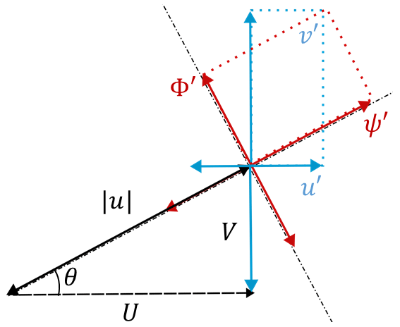
Figure C1 Graphical illustration of the conversion of perpendicular wind data (average wind vectors U and V, with root-mean-square fluctuations u^′ and v^′) into an average absolute wind speed $\left|u\right|$, root-mean-square fluctuation in the direction of the plume Φ^′, and the plume opening angle: ${\tan }^{-\mathrm{1}}\frac{{\mathrm{\Phi }}^{\prime }}{\left|u\right|}$.

Figure C2 Graphical illustration of the local geodetic coordinate system (XYZ) and wind-direction-aligned coordinate system (ξηz).

In order to allow the uncertainty analysis as explained in Sect. 3 for 2-dimensional curtain flights, the raw wind data need to be converted into an absolute wind speed and their root-mean-square fluctuation, as well as a plume opening angle. The conversion process is graphically illustrated in Fig. C1. The absolute wind speed $\left|u\right|$ is determined from the perpendicular components of the average wind vector, U and V, as follows: $\left|u\right|=\sqrt{U^{\mathrm{2}}+V^{\mathrm{2}}}$. The average wind direction from the east (in radians) is then computed from $\mathit{\theta }={\tan }^{-\mathrm{1}}\frac{U}{V}$. The root-mean-square fluctuations in the direction of the plume, ψ^′ in meters per second, can be computed from the fluctuations in the east–west and north–south directions denoted, respectively, by u^′ and v^′: ${\mathit{\psi }}^{\prime }=u^{\prime }\cos \mathit{\theta }+v^{\prime }\sin \mathit{\theta }$. The dimensionless fluctuations divided by the wind speed are given by $\frac{{\mathit{\psi }}^{\prime }}{\left|u\right|}$. The root-mean-square fluctuations perpendicular to the plume, Φ^′ (also in m s⁻¹), are then given by ${\mathrm{\Phi }}^{\prime }=-u^{\prime }\sin \mathit{\theta }+v^{\prime }\cos \mathit{\theta }$. Finally, the approximate opening angle of the plume in radians is given by ${\tan }^{-\mathrm{1}}\frac{{\mathrm{\Phi }}^{\prime }}{\left|u\right|}$.

Appendix D: A note on the interpolation of the concentration measurement

Table D1 Emission rates calculated per curtain using nearest-neighbor and Gaussian smoother interpolation techniques and the average emission rate between upward and downward curtains for measurement A, which was carried out on 13 November 2019. The emission rates in the table are calculated using Eq. (8). The true emission rate was 30.8 g h⁻¹.

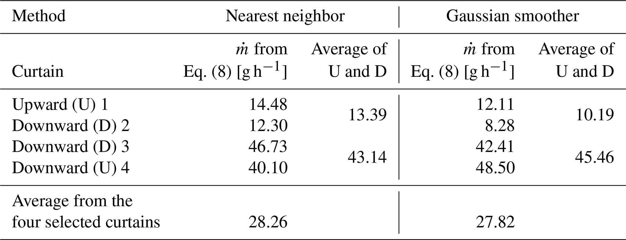
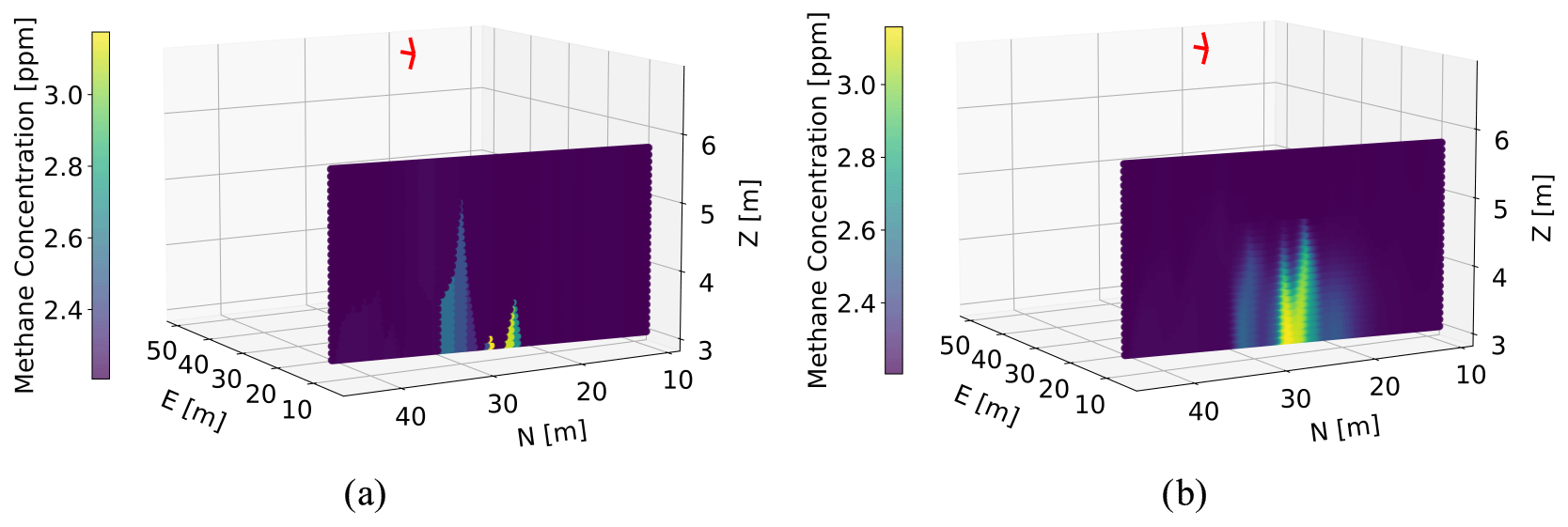
Figure D1 The 3-dimensional interpolated concentration values for upward curtain “1” (Fig. 8a) using (a) nearest-neighbor and (b) Gaussian smoother interpolation techniques. The red arrow indicates the average wind direction.

Figure D2 The 3-dimensional interpolated concentration values for downward curtain “2” (Fig. 8a) using (a) nearest-neighbor and (b) Gaussian smoother interpolation techniques. The red arrow indicates the average wind direction.

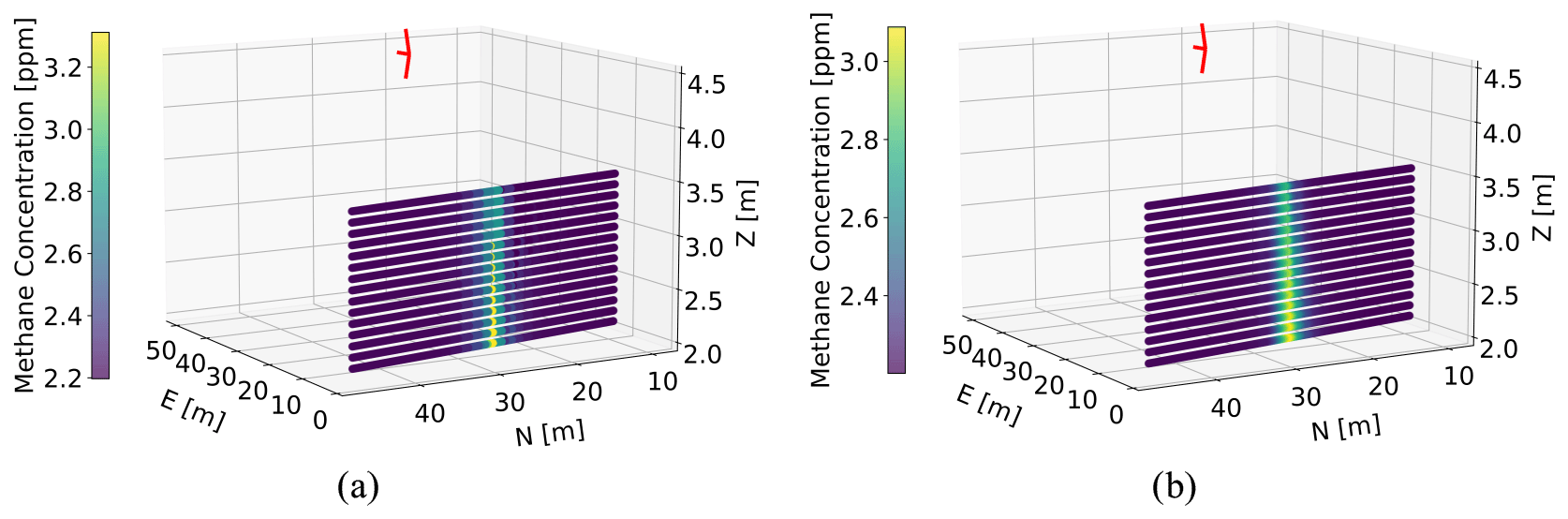
Figure D3 The 3-dimensional interpolated concentration values for downward curtain “3” (Fig. 8b) using (a) nearest-neighbor and (b) Gaussian smoother interpolation techniques. The red arrow indicates the average wind direction.

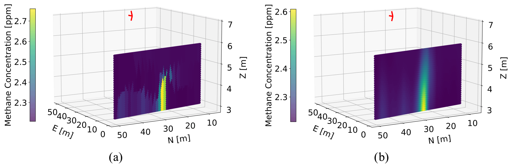
Figure D4 The 3-dimensional interpolated concentration values for upward curtain “4” (Fig. 8c) using (a) nearest-neighbor and (b) Gaussian smoother interpolation techniques. The red arrow indicates the average wind direction.

As mentioned in the main body, different approaches can be used to interpolate the concentration measurements on the plane. In Sect. 4.1, the nearest-neighbor method was used based on the fact that Scientific Aviation uses this interpolation technique. However, to assess the impact of the interpolation technique on the estimated emission rate, we compare here the results obtained from the nearest-neighbor method to those of the Gaussian smoother method. We follow the interpolation technique like a Gaussian smoothing function, as in Price (2012).

Shown in Figs. D1, D2, D3, and D4 are the interpolated methane measurements on the plane for upward curtain “1” (Fig. 8a), downward curtain “2” (Fig. 8b), downward curtain “3” (Fig. 8c), and upward curtain “4” (Fig. 8d), respectively, using (panel a) the nearest-neighbor and (panel b) the Gaussian smoother interpolation techniques. As seen the Gaussian smoother provides a smooth transition between high and low concentration values due to its nature. However, if the plume is missed, the Gaussian smoother cannot recover the missing high concentrations, as apparent in the bottom of the plane in Fig. D1 and the top of the plane in Fig. D2.

Presented in Table D1 are the emission rates calculated per curtain using the nearest neighbor and Gaussian smoother and the average emission rate between upward and downward curtains. The maximum difference between the emission rates estimated for the four curtains using the two interpolation methods is 8.40 g h⁻¹, and the impact of the average emission rate is 0.44 g h⁻¹ (1.4 % of the total emission rate of 30.8 g h⁻¹).

Our tentative conclusion from the analysis presented in this section is that the choice of the interpolation method has a relatively small impact on the mass emission estimate. Moreover, some sources of error cannot be compensated for by a different choice of interpolation method: if the highest-concentration enhancements are not measured because of a large vertical spacing between flight lines, then the resulting estimate for the mass emission rate will underestimate the true mass emission rate – regardless of the mapping technique employed.