Detection and quantification of methane plumes with the MethaneAIR airborne spectrometer

The MethaneAIR imaging spectrometer was originally developed as an airborne demonstrator of the MethaneSAT satellite mission. MethaneAIR enables accurate methane concentration retrievals from high-spectral-resolution measurements in the 1650 nm methane absorption feature at a nominal spatial sampling of 5 × 25 m. In this work, we present a computationally efficient data processing chain optimized for the detection and quantification of methane plumes with MethaneAIR. It involves the retrieval of methane concentration enhancements (ΔXCH₄) with the high-precision matched-filter retrieval, which is applied to 1650 nm retrievals for the first time. Methane plumes are detected via visual inspection of the resulting ΔXCH₄ maps. We evaluated the performance of this processing scheme with simulated plumes, intercomparison with other methods, and controlled methane releases. We applied this processing chain to MethaneAIR data mosaics acquired over the Permian Basin during flights in 2021 and 2023, which resulted in the detection of hundreds of point sources above 100–200 kg h⁻¹, with a conservative detection limit of around 120 kg h⁻¹. Our results show the consistency of MethaneAIR's ΔXCH₄ matched-filter retrievals as well as their potential for the detection and quantification of methane point sources across large areas.

1 Introduction

The remote detection and quantification of methane emissions from small infrastructure elements, also known as point sources, is crucial to guide methane emission mitigation efforts. Airborne and spaceborne imaging spectrometers are being widely used for this application. Optical imaging spectrometers record the light reflected by the Earth surface after interaction with the atmosphere in hundreds of contiguous spectral channels. These spectrally resolved measurements allow the quantification of atmospheric methane concentrations from the 1650 or 2300 nm shortwave infrared (SWIR) spectral regions in which methane absorbs radiation. The resulting methane concentration maps can be used to identify and quantify methane plumes, which can be attributed to the corresponding sources.

We can classify the imaging spectrometers with potential for methane mapping into two different instrument classes, defined by the instrument's spectral configuration. First, we have the spectrometers sampling the entire solar spectrum (∼ 400–2500 nm) with a relatively coarse spectral sampling of between 5 and 10 nm and a relatively high spatial resolution (a few metres in the case of some airborne instruments). Methane retrievals for this type of instrument exploit the 2300 nm methane feature. Most of the developments towards the detection and quantification of methane point sources are based on previous work with the AVIRIS and AVIRIS-NG airborne spectrometers, which belong to this instrument class. For example, Roberts et al. (2010) detected methane emissions from a marine geological seep source with AVIRIS; Thorpe et al. (2014, 2017) discussed methane retrieval methods for AVIRIS and AVIRIS-NG; Frankenberg et al. (2016) used AVIRIS-NG to survey methane point sources in the Four Corners region (USA); and Cusworth et al. (2022) assessed the methane emissions from different US basins with AVIRIS-NG.

The second group of methane-sensitive spectrometers sample a narrow spectral window around the 1650 nm methane absorption, with a sub-nanometer spectral sampling and a typically coarser spatial sampling. The GHGSat instruments (spaceborne and airborne) and the Methane Airborne MAPper (MAMAP) and MAMAP-2D airborne spectrometers belong to this category. The 1-D (profiler) version of the MAMAP spectrometer has been operating since the 2010s (Krings et al., 2011). For example, MAMAP was used to map methane emissions in the Upper Silesian Coal Basin in southern Poland (Krautwurst et al., 2021). A 2-D configuration (imager) of the instrument is now available (Gerilowski et al., 2011). In general, the instruments sampling a narrow spectral window around the 1650 nm absorption with a high spectral resolution can better disentangle the methane signal from that of surface structures. This makes these instruments less affected by surface-driven systematic retrieval errors, although this usually comes at the expense of a higher retrieval noise.

The MethaneAIR instrument belongs to the spectrometer class sampling the 1650 nm window. It was developed as the airborne demonstrator of the MethaneSAT satellite mission, launched on 4 March 2024 (Environmental Defense Fund, 2021). Unlike other airborne imaging spectrometers solely used for point sources, MethaneAIR is intended to provide information on both high-emitting point sources and area sources and, subsequently, on total regional emissions. To achieve its primary goals of total regional emission quantification, MethaneAIR is designed to fly at high altitudes (typically about 12 000 m above ground). This allows one to map wider areas faster while also disaggregating emissions from area and point sources, at the expense of some loss in spatial resolution compared to airborne systems flying at lower altitudes. In addition, the need to sample area sources motivates the implementation of an accurate methane concentration (XCH₄) retrieval in MethaneAIR's operational processing chain that is based on the CO₂-proxy method (Chan Miller et al., 2024). The good performance of MethaneAIR's CO₂-proxy XCH₄ retrieval for the quantification of methane plumes has been shown in Chulakadabba et al. (2023) and El Abbadi et al. (2024). However, this retrieval is computationally demanding. Moreover, the normalization of the retrieved methane column density by the per-pixel XCO₂ proxy increases the 1σ error of the resulting XCH₄ maps, which may lead to higher plume detection limits.

In this work, we delve into maximizing the effectiveness of MethaneAIR measurements to rapidly process data across large areas with the goal of improving plume detection limits. We propose a data processing scheme optimized for the detection of methane plumes, namely, through a high-precision data-driven methane concentration retrieval based on the matched-filter concept and on the visual inspection of the resulting methane concentration maps. We tested this processing chain on large-scale flight campaigns performed with MethaneAIR over the Permian Basin (USA) as well as over a controlled-release experiment in Arizona (USA) in recent years.

2 Materials and methods

2.1 MethaneAIR's specifications and data products

An overview of the MethaneAIR instrument and a list of its technical specifications are provided in Staebell et al. (2021). MethaneAIR is typically flown at a 12 km altitude, which leads to a swath width of about 7.5 km, with an across-track pixel size of about 5 m and an along-track pixel size of 25 m. MethaneAIR's methane band covers the 1592–1680 nm window, with a spectral resolution (full width at half maximum of the spectral response function) of about 0.3 nm and a spectral sampling of 0.1 nm. As is shown in Fig. 1, it samples the methane absorption feature around 1650 nm and the CO₂ absorption feature around 1610 nm, the latter of which is used for the CO₂-proxy methane retrieval (Chan Miller et al., 2024).

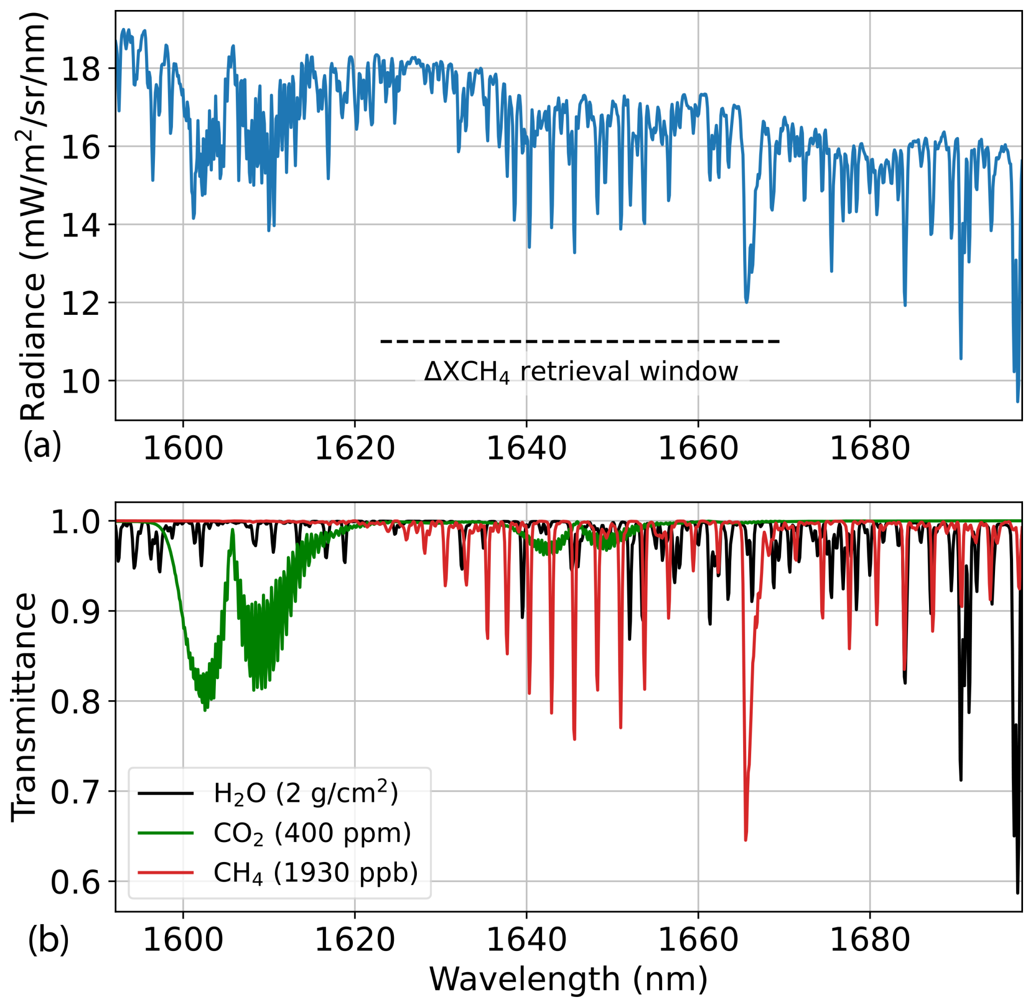
Figure 1 MethaneAIR's spectral coverage and sensitivity to atmospheric gases. A real MethaneAIR at-sensor radiance spectrum is shown in panel (a). The spectral window used for the retrieval of methane concentration enhancements (ΔXCH₄) in this work is depicted with a dash line. Spectral transmittance spectra for methane, CO₂, and water vapour convolved with MethaneAIR's spectral response functions are displayed in panel (b). A nadir observation and a Sun zenith angle of 25° are assumed. The column contents of each gas are displayed in the legend.

The conversion of MethaneAIR's raw level-0 data into level-1B spectral radiance data cubes is described in Conway et al. (2024). Subsequent processing levels in MethaneAIR's operational processing chain include dry-air column methane mixing ratio (XCH₄) maps in the original instrument coordinates as the level-2 product (Chan Miller et al., 2024), geoprojected and orthorectified XCH₄ mosaics as the level-3 product, and information on methane fluxes (both detected plumes from high-emitting point sources and spatially distributed areal fluxes) as the level-4 product.

As input, this study uses MethaneAIR level-1B data, which correspond to calibrated and georeferenced radiance spectra. MethaneAIR's level-1B spectral radiance datasets are stored as “granules” of 301 × 1280 spatial pixels (along the track × across the track). The full flight line is reconstructed after appending all granules in the along-track direction. For the across-track direction, 1280 is the size of the detector's focal plane array, but only a fraction of it (typically, 863 pixels) is illuminated. When the data are spatially binned across the track (5 spatial pixels combined into 1) in order to generate lighter data files with square pixels, the dimensions of the illuminated part of a single granules is 301 × 172 pixels (7.5 km along track and 4.7 km across track, for nominal operations at a 12 km altitude).

2.2 ΔXCH₄ retrieval

A useful variable for the detection and quantification of methane point sources from remote-sensing data is the per-pixel methane concentration enhancement (ΔXCH₄). For the retrieval of ΔXCH₄ maps with MethaneAIR, we have adapted the matched-filter retrieval. This has been widely applied to a range of airborne and spaceborne spectrometers sampling the 2300 nm methane absorption with a 5–10 nm spectral resolution (e.g. Thompson et al., 2015, 2016; Foote et al., 2020; Cusworth et al., 2021; Irakulis-Loitxate et al., 2021; Guanter et al., 2021; Roger et al., 2024), but it has not been previously tested on MethaneAIR-like spectrometers measuring in the 1650 nm window with a 0.1 nm spectral sampling.

The matched-filter retrieval expresses the input radiance spectra as the perturbation of an average radiance spectrum by a change in the methane column concentration. This is modelled as a so-called target spectrum, which represents the radiative transfer signal of a unit methane absorption. Following the notation by Thompson et al. (2016), if we name ΔXCH₄ as $\widehat{\mathit{\alpha }}$, the matched-filter takes the following form:

$$\begin{array}{}\text{(1)}& \widehat{\mathit{\alpha }}\left(\mathit{x}\right)={\displaystyle \frac{{\left(\mathit{x}-\mathit{\mu }\right)}^T{\mathbf{\Sigma }}^{-\mathrm{1}}\mathit{t}}{{\mathit{t}}^T{\mathbf{\Sigma }}^{-\mathrm{1}}\mathit{t}}},\end{array}$$

where x is the spectrum under analysis, μ and Σ are the respective mean and covariance of the background spectral radiance, and t is the target spectrum representing the perturbation of the background radiance signal by a methane enhancement. The t spectrum has units of radiance over methane column concentration, and it is generated as μ⋅k, with k being a unit methane absorption spectrum calculated using radiative transfer simulations.

The variable μ is calculated on a per-column basis in order to account for the different radiometric responses of detector elements across the track. We acknowledge that this per-column μ formulation neglects the impact of difference between each pixel’s spectral albedo and μ. This issue may be alleviated by the albedo correction proposed by Foote et al. (2020), which adds an “albedo factor” to Eq. (1) in order to quantify the difference between μ and x for each pixel. The magnitude of this correction will depend on the spatial heterogeneity of the scene. Preliminary tests show that this correction can modify the single ΔXCH₄ retrievals by up to 10 % in the Permian (results not shown). However, the sign of the correction can be either positive or negative depending on the albedo of the surface (or surfaces) crossed by a particular plume. For this reason, we can expect that an uncorrected albedo effect may lead to an increase in the scatter of the estimated flux rates within a distribution, although it will not lead to a change in the total or the average flux rate of the distribution. In any case, we will implement this correction in a future version of the retrieval.

In the case of the target spectrum k, this is calculated at high spectral resolution from pre-computed transmittance spectra stored in a look-up table (LUT). For that, we interpolate the LUT considering the mean value of the Sun zenith angle and the ground-to-sensor distance within each data granule, whereas a per-column view zenith angle is used in order to account for across-track gradients in the observation angle. It must be stated that local gradients in surface elevation are not accounted for by this approach. The spectral convolution of the high-spectral-resolution k spectrum with MethaneAIR's spectral response function is also performed on a per-column basis in order to account for potential across-track variations in the instrument spectral response, as caused by e.g. changes in the thermal environment of the sensor. An initial step in our processing chain detects and corrects potential global spectral shifts in the MethaneAIR spectral calibration.

Regarding the inverse covariance matrix Σ⁻¹, it was calculated on a per-column basis in our first implementation of the retrieval. However, we noted that the relatively low number of along-track samples (301) in the level-1B data granules (see Sect. 2.1) affected the calculation of Σ⁻¹ so that the retrieval was biased low. This effect has also been found in the processing of short flight lines from the AVIRIS-NG sensor (Ayasse et al., 2023). To overcome this issue, we calculate a global Σ⁻¹ from all of the pixels in the granule, which proved to solve the underestimation of ΔXCH₄ while also being effective to account for across-track offsets thanks to the per-column calculation of μ. This granule-level Σ⁻¹ calculation is allowed by MethaneAIR's uniform spectral response in the across-track direction (very low spectral smile effect).

The 1623–1670 nm window was selected for the matched-filter retrieval, as it provides a good compromise between the number of methane lines available for the retrieval and the potential disturbance by other gases (see Fig. 1). Other narrower fitting windows were tested, but they yielded higher precision errors without a clear gain in retrieval accuracy.

2.3 Plume detection and quantification

Methane plumes are detected through visual inspection of the ΔXCH₄ maps generated from each level-1B granule, following the approach described in Guanter et al. (2021) for the PRISMA spaceborne spectrometer. In short, the candidate plumes identified through a first screening based on visual inspection are compared with the input spectral radiance data at the continuum of the 1650 nm absorption feature to discard false positives due to surface patterns (e.g. clouds). However, thanks to MethaneAIR's high spectral resolution, the large majority of the plumes that we derived from MethaneAIR were clear enough to have confidence in the detection, making the need for cross-checking with very high resolution imagery very small.

The relatively low sensitivity of MethaneAIR ΔXCH₄ retrievals to the background surface would allow one to implement an automatic detection process for the larger plumes using thresholds on ΔXCH₄ or machine learning segmentation and classification methods (e.g. Joyce et al., 2023; Růžička et al., 2023). However, we opted for the manual approach in order to ensure that the maximum number of plumes was properly detected. This method also minimizes the occurrence of false positives.

For the estimation of emission rates (Q) from the detected plumes, we use the integrated mass enhancement (IME) approach (Frankenberg et al., 2016; Varon et al., 2018). Following the mass-balance principle, the total mass enhancement in the plume is related to the magnitude of the emission with a parameterization dependent on wind speed, as follows:

$$\begin{array}{}\text{(2)}& Q={\displaystyle \frac{U_{\mathrm{eff}}\cdot \text{IME}}{L}},\end{array}$$

where the plume length L is approximated by the square root of the detectable plume. This model calculates an IME in kilogram units as the total excess mass of methane contained in the plume. Plumes are manually delineated in the ΔXCH₄ maps using a Python script that has been implemented for this purpose. As proposed by Varon et al. (2018), we use an effective wind speed (U_eff) in order to account for eddy-scale turbulence at the MethaneAIR's spatial resolution, combined with the effects of retrieval noise. This U_eff is related to the 10 m wind speed U₁₀ as follows:

$$\begin{array}{}\text{(3)}& U_{\mathrm{eff}}=\mathrm{0.34}\cdot U_{\mathrm{10}}+\mathrm{0.42}.\end{array}$$

This relationship was proposed by Maasakkers et al. (2022) for GHGSat for surface-level emissions (landfills in their case). GHGSat and MethaneAIR share a similar spatial resolution (∼ 25 m) and a comparable retrieval noise (both instruments rely on high-spectral-resolution measurements in the 1650 nm window). U₁₀ data are taken from the GEOS-FP meteorological reanalysis product (GEOS-Chem, 2024). Errors in Q estimates are obtained from the propagation of ΔXCH₄ retrieval errors and a 50 % uncertainty in wind speed through Eq. (2). The 50 % uncertainty in wind speed is chosen as a conservative estimate for this variable, which drives the uncertainty in Q estimations.

2.4 Reference plume quantification methods

We have intercompared our Q estimates from the IME model with those from the modified IME (mIME) model and the divergence integral (DI) Q estimation method. Both were developed for MethaneAIR and have been thoroughly validated with controlled-release tests (Chulakadabba et al., 2023).

The mIME model was proposed by Chulakadabba et al. (2023). They assumed a logarithmic dependence between U_eff and U₁₀. For U₁₀, they used the 10 m root-mean-square wind obtained from each large-eddy simulation (LES) realization specifically run for the case of interest, rather than relying on operational meteorological products. However, we have chosen a more simple approach based on GEOS-FP winds, as we have to run the Q estimates for a large number of plumes.

For the DI method, we calculate the fluxes along rectangular boxes around the source of interest. First, we compute the flux for each pixel along the chosen rectangular box. We then determine the gradient of XCH₄ and multiply it by the wind vector at each pixel. Based on Green's theorem, we sum all of the fluxes to obtain the total flux for a given rectangle. By repeating this calculation for rectangles of different sizes around the source, we obtain a statistical estimate of the flux around the source of interest. In other words, we sample the flux spatially across the observing region using the DI method. Unlike the IME method, we neither sum all of the pixels within the plume nor use an effective wind speed.

These two Q estimation methods are more challenging to run over a large number of plumes than our basic IME method, but they can provide an ideal reference to assess the performance of our simple IME-based Q estimates.

2.5 End-to-end simulations of ΔXCH₄ retrievals

We have used simulations to assess potential retrieval biases. We embedded simulated methane plumes into real MethaneAIR level-1B data cubes. The simulated plumes were generated with the LES extension of the Weather Research and Forecasting model (WRF-LES). Concentrations in WRF-LES plumes were scaled to recreate a range of Q values.

The spatially distributed ΔXCH₄ values from the simulated plumes were converted into per-pixel plume transmittance spectra with the same LUTs used for the generation of the k spectrum, which is an input to the ΔXCH₄ retrieval. With this approach of using the same radiative transfer scheme for the forward simulations and for the ΔXCH₄ retrieval, we avoid introducing uncontrolled systematic errors in the end-to-end simulation framework (e.g. as from different gas vertical profiles).

This mixed forward simulation approach combining real radiance data with simulated plumes has already been used for the sensitivity analysis of high-resolution methane-sensitive instruments (Guanter et al., 2021; Roger et al., 2024; Gorroño et al., 2023). The use of real radiance data ensures that the actual measurement noise and potential radiometric and spectral offsets are intrinsically included in the simulation.

2.6 MethaneAIR datasets used in this study

We evaluated MethaneAIR's potential for surveying methane point sources across large oil and gas basins using level-1B data from several MethaneAIR flight campaigns. In this work, we report results from the analysis of two MethaneAIR research flights focused on the Permian Basin (USA), where a high concentration of active methane sources can be found. Those Permian Basin flights took place on 6 August 2021 (“RF06” flight) and on 20 July 2023 (“MX025” flight), and covered a region of about 120 × 80 km², including the Delaware sub-basin of the Permian Basin's oil and gas field, with flights longer than 2 h.

In addition, we processed data from two other research flights, RF01E and RF03E, that were carried out on 25 and 29 October 2022 over a single-blind volume-controlled methane-release experiment near Phoenix (USA) (Chulakadabba et al., 2023). We only considered the plumes entirely contained in a MethaneAIR granule (as opposed to plumes located at the intersection between two granules). This resulted in 16 match-ups between MethaneAIR acquisitions and controlled releases. We observed that the winds during the 29 October campaign were less consistent and had a poor alignment with different observational sources and model outputs.

3 Results

3.1 ΔXCH₄ retrieval performance

Results from the processing of a sample data granule of the RF06 campaign are displayed in Fig. 2, which shows a map of the input at-sensor radiance at 1623 nm (shortest wavelength in the retrieval window; see Fig. 1) as well as the corresponding ΔXCH₄ map. The processing involved ΔXCH₄ retrieval, plume detection, and Q estimation using the IME model. Four plumes were detected through the visual inspection process, with Q values ranging from 87 ± 33 to 512 ± 180 kg h⁻¹. It can be observed that these four plumes clearly stand above the background noise, although an automatic detection and segmentation of the smaller plumes would have been challenging. It can also be seen that there is a very low occurrence of systematic outliers in the ΔXCH₄ maps despite the relatively high variability in the surface patterns, unlike the case of coarser-spectral-resolution instruments (Jongaramrungruang et al., 2021).

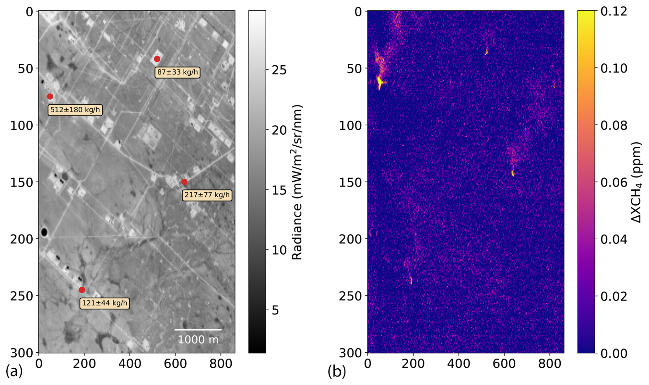
Figure 2 ΔXCH₄ map retrieved from a MethaneAIR data granule from the RF06 Permian campaign. A map of the at-sensor radiance at 1623 nm is shown in panel (a), and the retrieved ΔXCH₄ map is displayed in panel (b). The red points and the text boxes on the radiance map depict the location and flux rate of the four plumes detected in this subset.

We expect that MethaneAIR's high spectral resolution enables a better decoupling of methane and surface reflectance in the retrieval than what is usually found in coarser-spectral-resolution retrievals (Ayasse et al., 2018). Further insights into the impact of the surface reflectance and spatial heterogeneity on the retrieval are provided in Fig. 3. It compares the intensity and spatial variability in the at-sensor radiance with those of the retrieved ΔXCH₄ for selected granules from the RF06 and RF01E flights during which no methane plumes were detected. The spatial sampling is MethaneAIR's native 5 × 25 m sampling. The results show that the ΔXCH₄ variability is very close to a normal distribution, even for the RF01E granule for which the input radiance was far from Gaussian. The standard deviation is 33 and 38 ppb (parts per billion) for the RF06 and RF01E granules, respectively. We interpret those numbers as the retrieval 1σ error for those granules. This 1σ error combines the per-pixel retrieval noise (measurement noise propagated to ΔXCH₄ retrieval noise for each input spectrum), the variability introduced by the sensitivity of the retrieval to the surface spectral reflectance, and the potential contribution of methane sources in or close to the data granule under analysis. The lower 1σ error is found for the RF06 granule, which is consistent with the higher and more spatially uniform at-sensor radiance. However, it must be remarked that the Permian Basin presents a high concentration of methane point sources, so it is possible that part of the variability captured in the σ calculated for the RF06 granule is due to methane plumes outside the analysed granule or below MethaneAIR's detection limit.

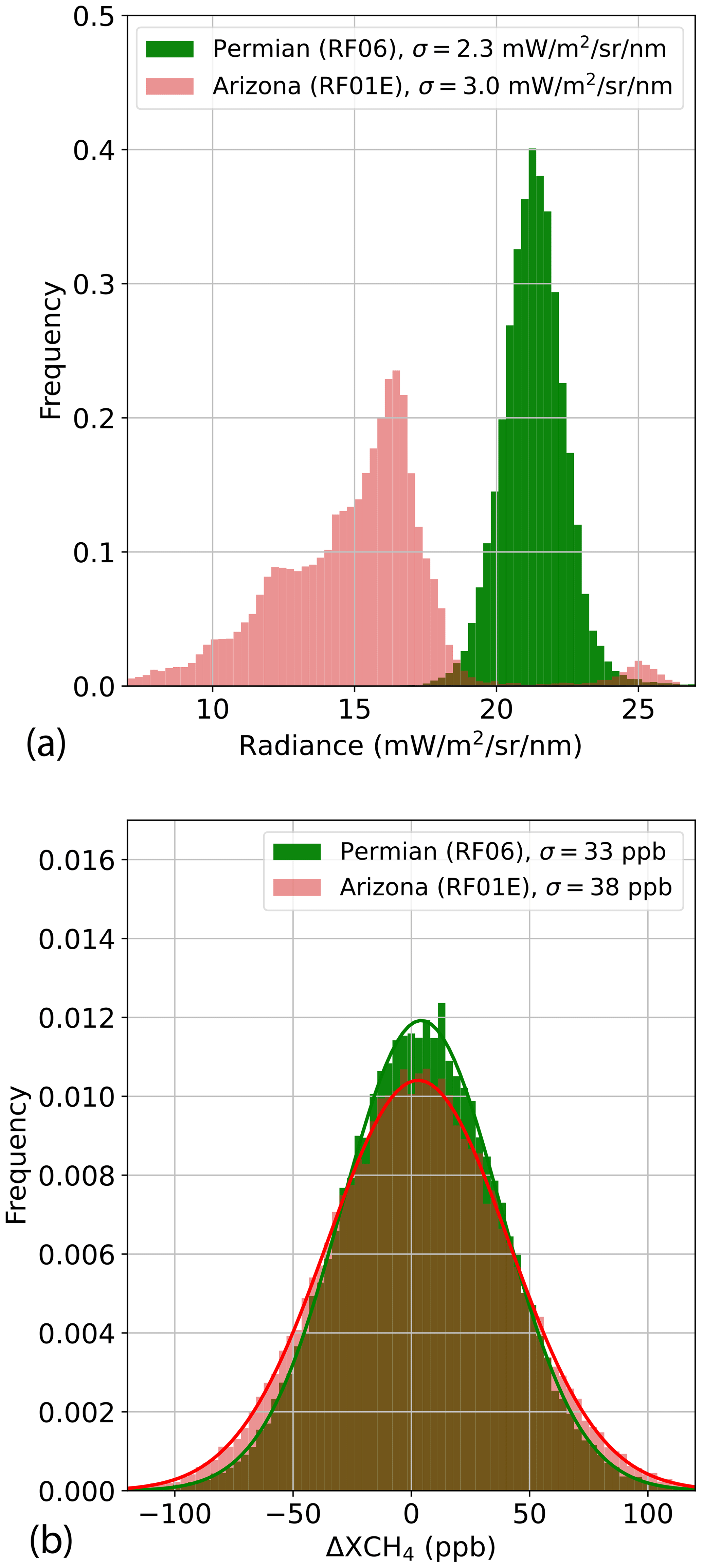
Figure 3 Variability in at-sensor radiance at 1623 nm (a) and retrieved ΔXCH₄ (b) for sample subsets from the Permian Basin and Arizona campaigns (RF06 and RF01E, on 6 August 2021 and 25 October 2022, respectively).

A comparison between the matched-filter ΔXCH₄ retrieval and the CO₂-proxy XCH₄ retrieval implemented in MethaneAIR's operational processing chain is shown in Fig. 4 for a subset of the granule displayed in Fig. 2. ΔXCH₄ is calculated from the XCH₄ generated by the CO₂-proxy through the removal of the XCH₄ background, which is estimated as a single offset from the plume-free pixels in the subset. The comparison of the two retrievals shows that the ΔXCH₄ values from the data-driven matched-filter retrieval agree well with the more sophisticated CO₂-proxy XCH₄ retrieval, which has been thoroughly validated (Chan Miller et al., 2024). Two small clusters of pixels with systematic offsets corresponding to the larger plume can be seen in the difference map, at pixel coordinates (10, 60) and (10, 40). However, these enhancements are close to the noise level and have a different sign, leading to an almost zero offset when aggregated to calculate the IME and, subsequently, Q. Furthermore, we observe that the retrieval noise is lower for the matched-filter retrieval, namely, σ of 34 ppb for the CO₂-proxy retrieval and 23 ppb for the matched-filter, which enables the detection of a smaller plume on the right-hand side of the matched-filter map. Note that these numbers are for a 25 × 25 m sampling, whereas the σ values in Fig. 3 were for the native 5 × 25 m sampling. The higher retrieval precision error of the CO₂-proxy retrieval can be explained by the fact that the per-pixel normalization of the methane retrieval by the retrieved per-pixel CO₂ column density adds noise to the methane product. From this comparison, we conclude that the ΔXCH₄ maps generated with the matched-filter retrieval can lead to lower plume detection limits than the CO₂-proxy retrieval because of their higher signal-to-noise ratio, without an observable drop in retrieval accuracy. Nevertheless, physically based total-column XCH₄ retrievals from the CO₂-proxy (as opposed to the data-driven ΔXCH₄ retrievals by the matched-filter) are preferred for the estimation of area- and total-emission budgets, which is a key application of MethaneAIR. A physically based pixel-wise XCH₄ retrieval can better account for spatial gradients in the methane background caused by atmospheric transport and topography. This implies that the matched-filter ΔXCH₄ output is currently not an alternative to the CO₂-proxy XCH₄ retrieval for the calculation of area and total methane fluxes from MethaneAIR data cubes.

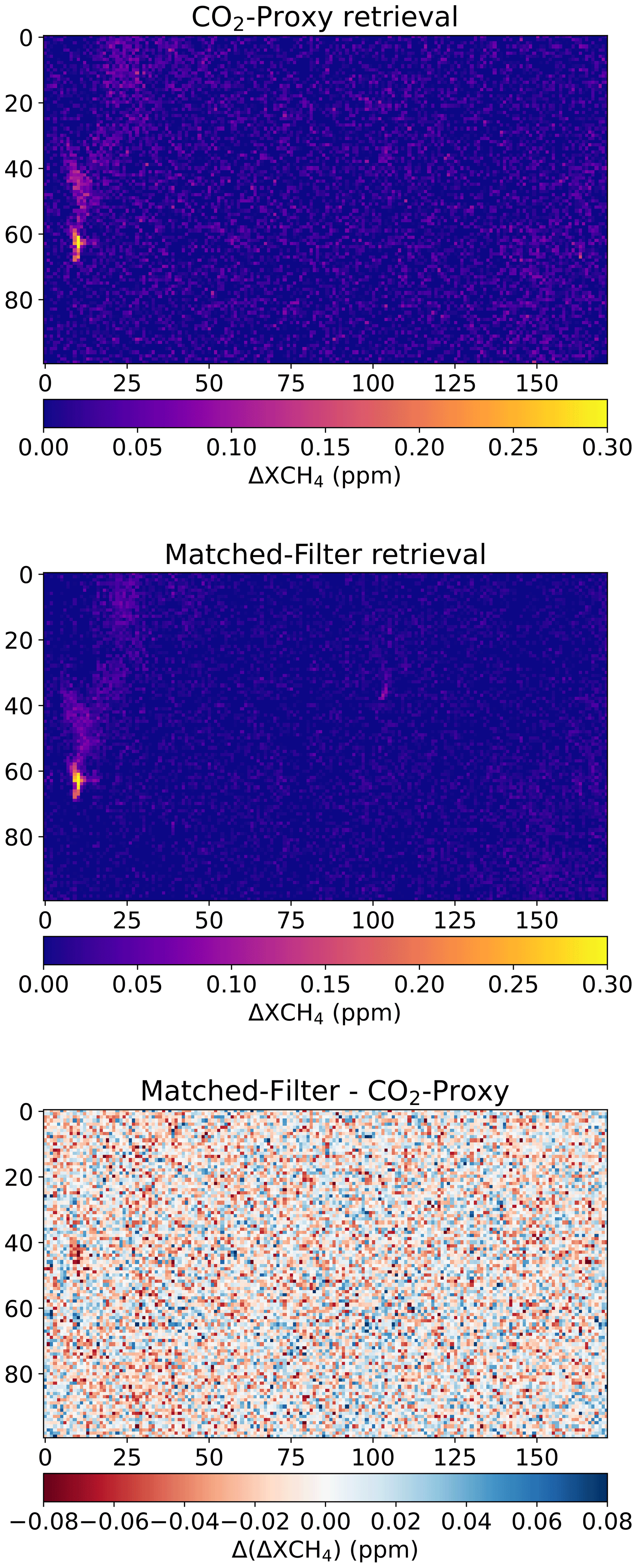
Figure 4 Comparison of ΔXCH₄ maps generated with MethaneAIR's official CO₂-proxy retrieval and the matched-filter retrieval proposed in this study. For the CO₂-proxy XCH₄ retrieval, the ΔXCH₄ map is generated as the per-pixel methane column mixing ratio (XCH₄) minus its mean value.

We have further tested the consistency of the matched-filter ΔXCH₄ retrievals by means of simulated plumes. A comparison between the input and the retrieved methane concentration enhancement from a simulated plume (Q = 500 kg h⁻¹, U₁₀ = 3.4 m s⁻¹) is shown in Fig. 5. The plume was embedded into a real MethaneAIR granule following the procedure described in Sect. 2.5. There is a good agreement in the peak ΔXCH₄ values between the simulated and the retrieved plume, which is evidenced by the lack of spatial structures in the difference map on the right-hand side of Fig. 5. On the other hand, the effect of retrieval noise is relatively large, causing some of the lower methane concentration patches within the plume fall below the noise level. This needs to be considered when assessing potential error sources in the Q estimation process. This issue is partly alleviated by the IME $/$ L ratio in the IME model (Eq. 2), which reduces the impact of missing pixels in the masked plume, and by the U_eff term (Eq. 3), which is generated using realistic estimates of the retrieval noise.

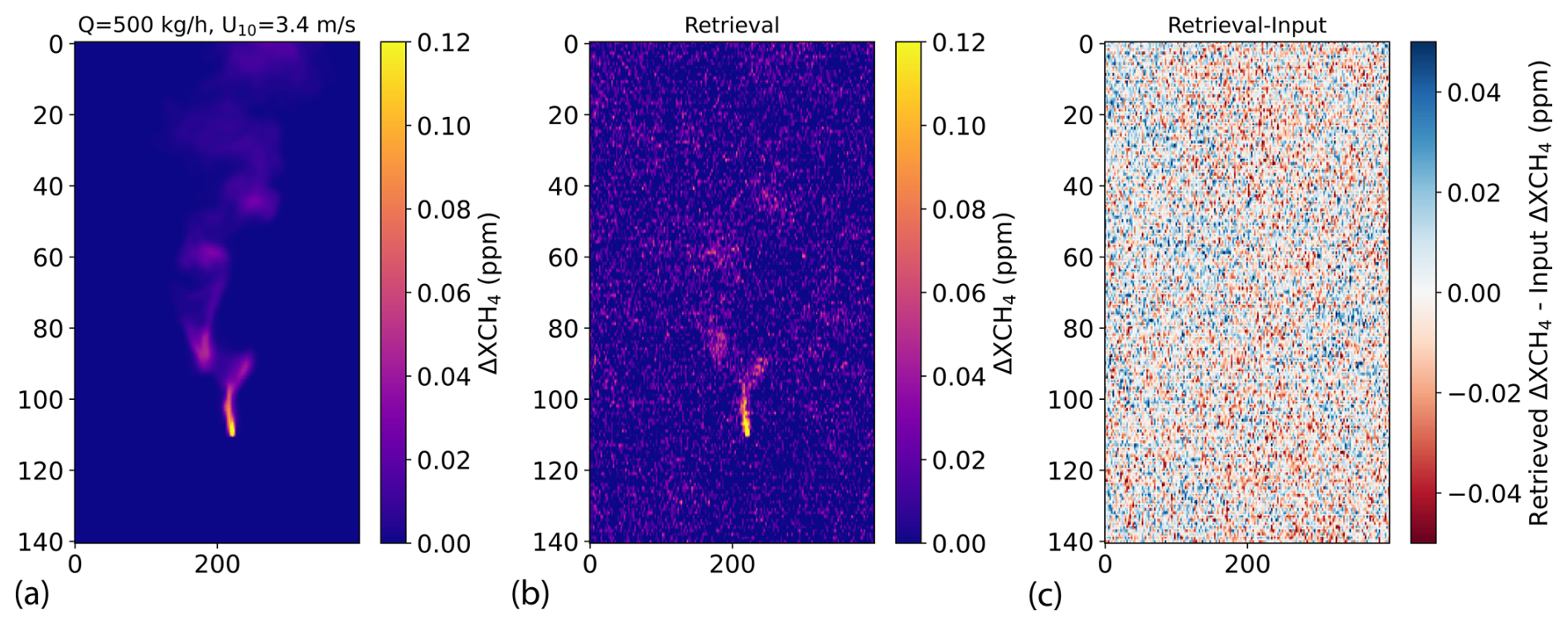
Figure 5 Results from end-to-end ΔXCH₄ retrieval simulations for a Q = 500 kg h⁻¹ plume embedded in a Permian Basin data granule from the RF06 campaign. The input WRF-LES plume is displayed in panel (a), the retrieved ΔXCH₄ map is shown in panel (b), and the difference between the two is given in panel (c).

3.2 Quantification of emission rates

The first test for the evaluation of the IME-based Q quantification method consisted of a comparison with the divergence integral (DI) method described in Chulakadabba et al. (2023). We generated Q estimates for a subset of 12 plumes from the RF06 campaign with the two methods. The same ΔXCH₄ maps from the matched-filter retrieval were used as an input for the two methods, but each method was constrained with different wind data: the IME-based method was run with GEOS-FP data, as this is the configuration that we apply for the processing of the large plume datasets derived in this work, whereas the DI method was constrained with HRRR wind data, as this is the configuration that potentially provides the most accurate reference for intercomparison with the IME approach.

The results from the quantification of the 12 plumes by the two methods are displayed in Fig. 6. Despite the different fundamental basis and wind data used by the two methods, we find a relatively good agreement in the quantification of those selected plumes, with differences in Q typically being below 20 % for most of the plumes. As the DI Q estimation method has been thoroughly validated through independent controlled-release tests (El Abbadi et al., 2024), this good agreement between the two methods suggests that our implementation of the IME model for MethaneAIR, constrained with GEOS-FP winds, can reproduce the emission rates for the conditions of the RF06 Permian Basin campaign.

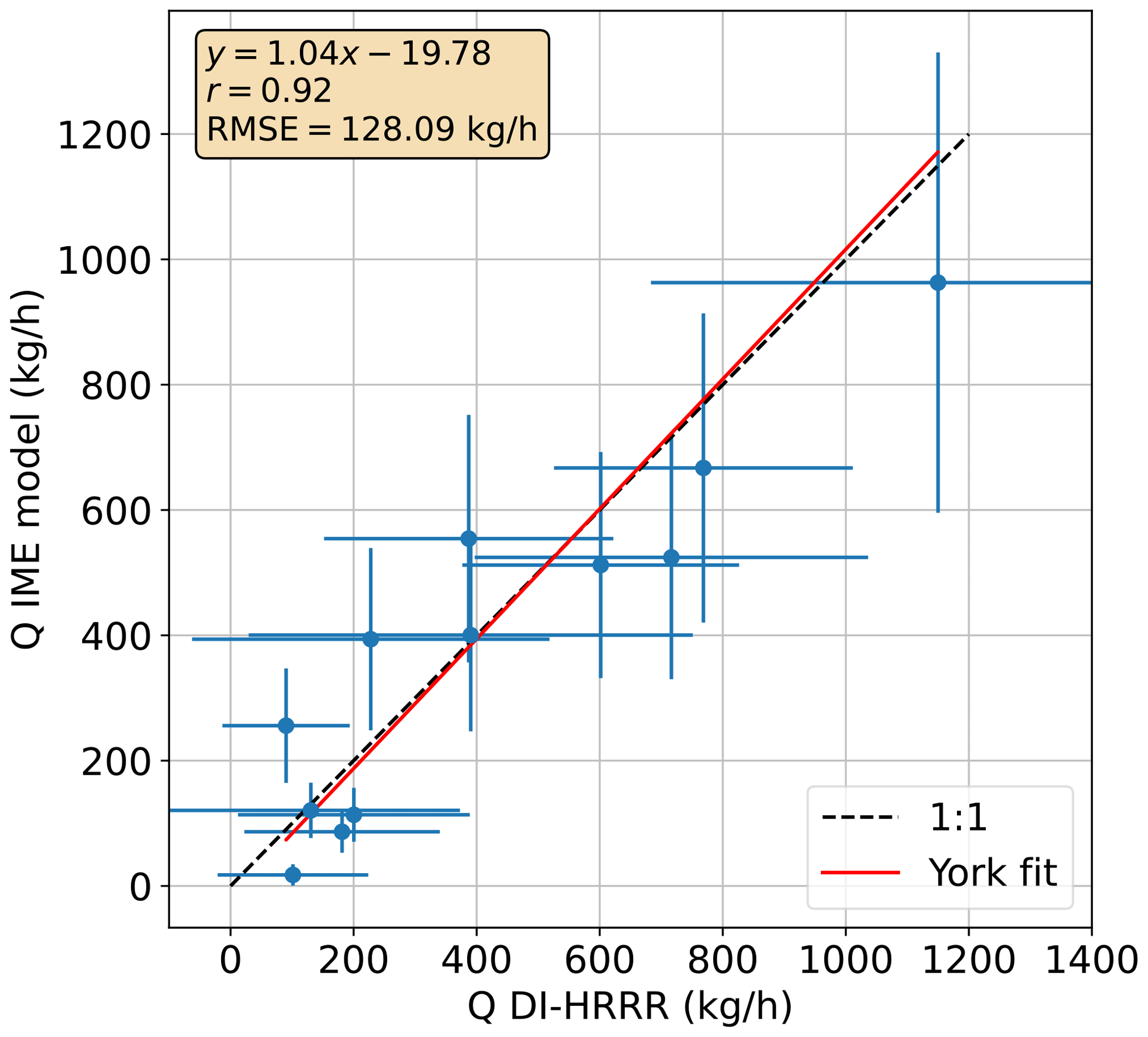
Figure 6 Comparison between Q estimates obtained with the IME-based model used in this work (see Sect. 2.3) and the divergence integral method (DI) described in Chulakadabba et al. (2023) (see Sect. 2.4) for 12 selected plumes from the RF06 campaign. Error bars represent the 1σ error for the IME Q estimates and the 95 % confidence interval for the DI estimates.

In order to further validate the plume detection and quantification skill of our processing chain, we have processed several MethaneAIR acquisitions over a controlled-methane-release experiment on 25 October 2022 in Arizona (USA) (RF01E campaign; see Sect. 2.6). Results from the ΔXCH₄ maps for three of the weakest releases detected during this experiment (metered values of 205, 96, and 63 kg h⁻¹) are shown in Fig. 7. Each map covers an area of about 2.5 km ×2.5 km. The maps show that the methane enhancements stand out from the background in all three cases, without systematic retrieval artefacts being present in the vicinity of the plume. Approximately the same number of pixels is affected by ΔXCH₄ values above the noise level for the Q = 63 kg h⁻¹ and Q = 96 kg h⁻¹ plumes. This could be due to the stronger wind during the weaker emission (0.9 m s⁻¹ versus 2.2 m s⁻¹, according to in situ measurements) causing a larger plume to originate close to the source, which implies that the probability of plume detection is not always inversely proportional to wind speed, but there is an optimal wind speed for plume detection in some cases: low-to-moderate winds enabled the development of a plume covering several pixels with ΔXCH₄ values above the noise level.

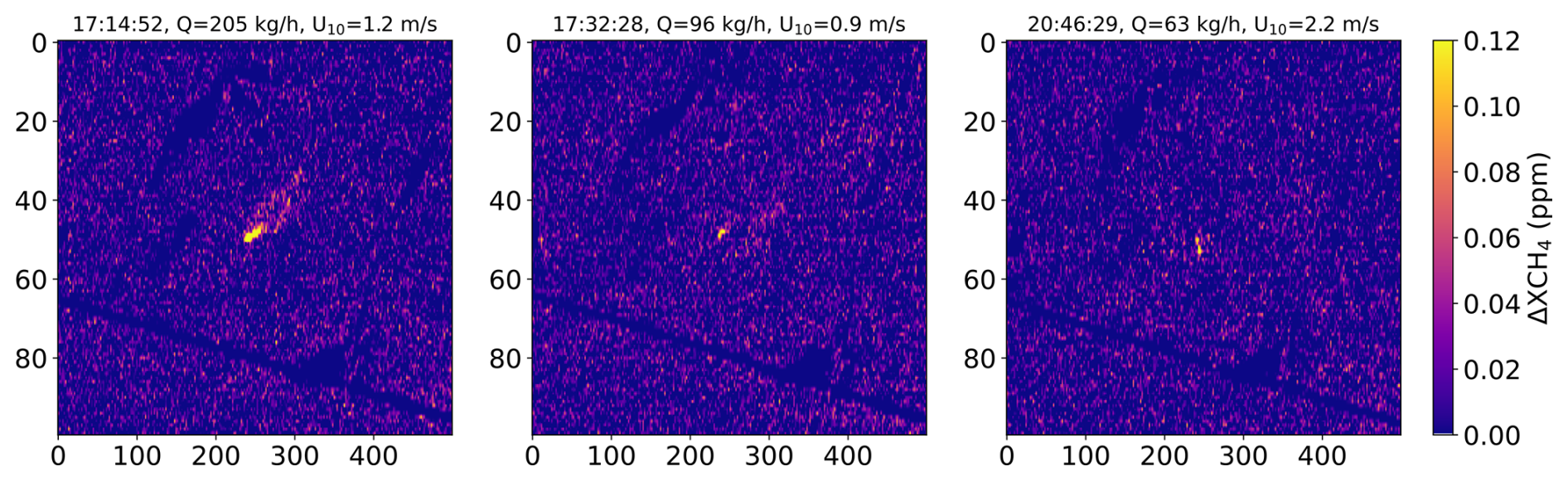
Figure 7 ΔXCH₄ maps over the controlled-methane-release experiment in Arizona on 25 October 2022. Overpasses corresponding to relatively weak emissions have been chosen. The flux rate (Q) and 10 m wind speed (U₁₀) in the title of each panel correspond to the metered values.

These results suggest that plume detection limits of about 60 kg h⁻¹ could be achievable with MethaneAIR flying at 12 km above the ground. However, two points must be noted. First, the location of the controlled-release site is known beforehand, so the identification of the enhancement and its confirmation as a real plume are much simpler in this case compared with the real case, where the location is unknown. Second, the plume detection process depends on several factors, including retrieval noise, occurrence of systematic errors, and wind speed. This means that the “minimum detection limit”, defined as the smallest source that can be detected in a given dataset, may substantially overestimate the plume detection capability of a sensor. The “probability of detection” concept leads to continuous probability of detection functions, which express the probability with which a plume of a given flux rate will be detected, and can better represent the variability in detection limits found under normal operating conditions (e.g. Conrad et al., 2023). We will continue this discussion in Sect. 3.4.

The metered Q values from the controlled releases were used for a first assessment of the performance of our IME-based Q estimation model. The comparison between the metered values and the Q estimates from our processing (matched-filter ΔXCH₄ retrievals and IME-based Q estimates constrained by GEOS-FP winds) are shown in Fig. 8. The results from MethaneAIR correlate well with the metered values for the two campaign dates (r = 0.98 and 0.94 for 25 and 29 October, respectively), for both high and low flux rate values (100–1000 kg h⁻¹ range), which gives confidence in the performance of our entire processing chain. However, we find an important overestimation of about 40 % in the MethaneAIR flux rate estimates from 29 October, which we attribute to the large overestimation of wind speed that we find in GEOS-FP with respect to the metered wind speeds for that date (Fig. 8). This poor performance of GEOS-FP winds for 29 October is consistent with the poor performance of other wind sources and WRF-LES simulations with respect to the reproduction of in situ winds for that date. A higher sampling density over this site and others with different surface and wind conditions would be needed to extract more solid conclusions about the performance of our processing chain, similar to the more comprehensive analysis presented in Chulakadabba et al. (2023) and El Abbadi et al. (2024).

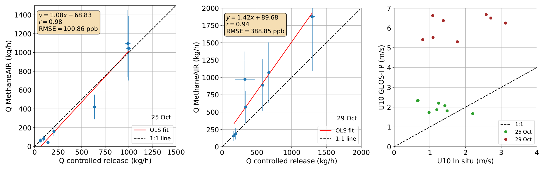
Figure 8 Comparison of metered flux rates from the controlled-release experiments in Arizona (25 and 29 October 2022) with flux rates estimated from MethaneAIR data using the processing chain described in this work. The metered flux rates correspond to 30 s averages. Error bars on the y axis represent the 1σ error for the IME Q estimates from MethaneAIR, while error bars on the x axis represent the standard deviation in the metered flux rate values in the 30 s window. The comparison of the wind speed (U₁₀) measured in situ with that retrieved from the GEOS-FP dataset for the two dates is also shown.

3.3 Attribution of plumes to sources

MethaneAIR's nominal operation mode provides a native pixel size of 5.76 × 25 m², which is larger than the 1–5 m spatial sampling range often found for airborne spectrometers (El Abbadi et al., 2024). This coarser spatial sampling is selected for MethaneAIR in order to increase the areal coverage of each overpass, which is required to evaluate areal fluxes as well as point sources. However, MethaneAIR's spatial sampling is still usually sufficient to attribute the detected plumes to their sources. This is illustrated in Fig. 9, which shows examples of methane plumes represented on top of at-sensor radiance maps from the same MethaneAIR acquisitions from which the ΔXCH₄ maps were derived. The analysis of the combined ΔXCH₄ and radiance maps is often sufficient to identify the facilities responsible for each emission. However, the combination with infrastructure databases, such as the Oil and Gas Infrastructure Mapping database (OGIM; Omara et al., 2023), and very high resolution optical imagery is needed to refine the information on the sources. Combining MethaneAIR radiance and ΔXCH₄ maps with those external data sources, we attribute the plumes in Fig. 9 to different infrastructure elements. For example, plume no. 1 comes from a complex well pad, plume no. 2 comes from a compressor station, plume no. 3 comes from a pipeline, and plumes nos. 4 to 7 come from processing plants.

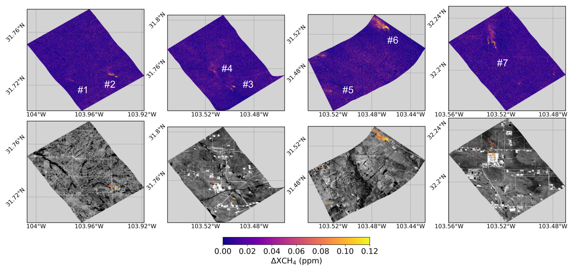
Figure 9 Sample methane plumes detected in ΔXCH₄ maps derived from data subsets from the MethaneAIR RF06 Permian Basin campaign. The raw ΔXCH₄ maps are shown in the top row, and the plumes represented on top of the radiance maps are presented in the bottom row. The numbers in white are used to refer to the different plumes in the text.

A zoomed-in view of Fig. 9's methane plume no. 7 is provided in Fig. 10. The plume is represented on top of a very high resolution satellite image downloaded from Google Maps. It is difficult to determine the exact source responsible for the emissions, but we discard the flare and the compressor units as potential sources because they are located elsewhere at the plant.

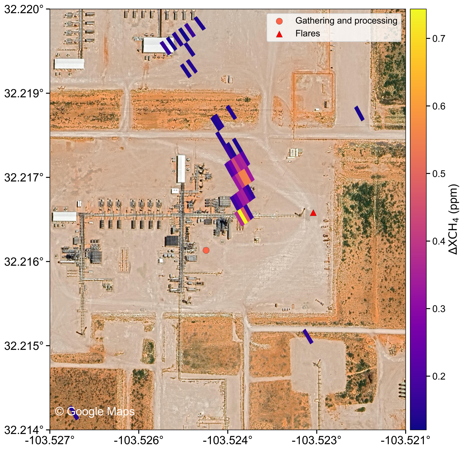
Figure 10 Methane plume from MethaneAIR represented on top of a high-resolution image showing the facility responsible for the emissions. The methane plume corresponds to plume no. 7 in Fig. 9. The background image was downloaded from © Google Maps and was acquired by Airbus in 2023.

3.4 Large-scale ΔXCH₄ mapping

We have assessed MethaneAIR's potential to survey methane point sources across large regions using entire flight lines from the RF06 and MX025 Permian Basin campaigns (see Sect. 2.6). The area covered by each flight (hundreds of kilometres in each case) is displayed in Fig. 11 using mosaics of near-infrared reflectance (at-sensor radiance at 1623 nm normalized by the top-of-atmosphere solar irradiance at the same wavelength). The detected methane sources and their intensity are depicted using red circles of varying size (see Tables S1 and S2 in the Supplement for the plume coordinates and flux rates for the RF06 and MX025 campaigns, respectively). It can be seen that the distribution of active sources varies considerably from one campaign to another, as shown by the area marked with the blue rectangle. We note that the RF06 and MX025 sampling areas cover some of the most active oil and gas production regions in the Permian, contributing more than one-third of the total Permian oil and gas production in 2023 (Enverus Prism, 2024). In addition, between 2021 and 2023, oil and gas production increased by 32 % and 40 % in RF06 and MX025, respectively. Furthermore, both RF06 and MX025 are active gas-flaring regions in the Permian. We suggest that such increased oil and gas activity could lead to increased emissions, plausibly due to increased stress on the gathering and processing segments, especially if their processing capacity did not increase accordingly.

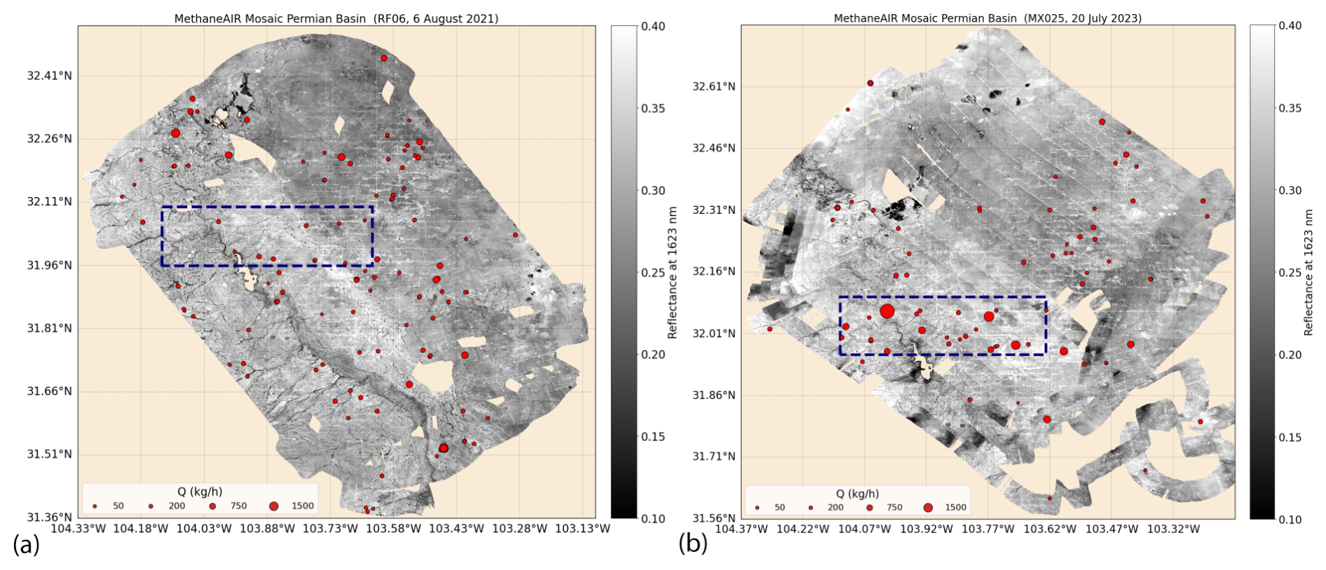
Figure 11 Composite of at-sensor reflectance data showing the areas in the Permian Basin covered by the MethaneAIR campaigns RF06 (a) and MX025 (b). At-sensor reflectance is calculated as the at-sensor radiance at 1623 nm normalized by the top-of-atmosphere solar irradiance at the same wavelength. The red circles depict the methane plumes detected for each campaign. The blue rectangle depicts an area with strong changes in emission activity between the two dates.

A more quantitative view of the detected points sources is provided in Fig. 12, which represents the distributions of emission rates obtained from all of the plumes that have been detected and quantified in the RF06 and MX025 datasets. This figure shows the higher number of plumes detected in the RF06 dataset compared with MX025 (121 and 78, respectively). We also find a difference in the minimum flux rates within each dataset, with the smallest flux rates in the range of 25 kg h⁻¹ for RF06 and 100 kg h⁻¹ for MX025 (see inset of Fig. 12), and that three plumes above 1500 kg h⁻¹ could be detected in MX025, although the number of plumes above 1000 kg h⁻¹ is similar for the two datasets (five for RF06 and six for MX025). Summing all of the flux rates, we obtain a total of 36 t h⁻¹ (metric tonnes per hour, 95 % CI of 30–42, where CI denotes confidence interval) for RF06 and 32 t h⁻¹ (95 % CI of 26–40) for MX025.

Figure 12 Summary of the flux rates (Q) estimated from the methane plumes detected in the RF06 and MX025 datasets (red circles in Fig. 11). The inset shows a zoomed-in view of the plumes with the smallest Q values. Uncertainties in the single Q estimates are not represented for visibility purposes.

These patterns are consistent with those found for the official MethaneAIR level-4 product made available to users (MethaneSAT Science Team, 2024); that is, a greater number of detections are noted in RF06, and higher flux rate peak values and detection limits are found in MX025 (29 plumes and a minimum flux rate of 228 kg h⁻¹ for RF06 compared with corresponding values of 19 and 492 kg h⁻¹ for MX025). The total emissions calculated from the level-4 dataset are 26.7 t h⁻¹ for RF06 and 25.6 t h⁻¹ for MX025, which is consistent with the 29 t h⁻¹ (95 % CI of 25–34) and 29 t h⁻¹ (95 % CI of 23–36) that we obtain from our dataset after filtering for plumes with flux rates above 200 kg h⁻¹. On the other hand, when using all of the detected plumes in our quantification of total emissions (i.e. without filtering out plumes < 200 kg h⁻¹), we obtain an increase in the total emission estimate of about 9 t h⁻¹ (RF06) and 6 t h⁻¹ (MX025) with respect to the level-4 product. This result confirms the sensitivity of the total emission estimates from single plumes to the detection limits offered by the instrument and the processing chain, and it suggests that smaller plumes contribute substantially to the totals despite the typical heavy-tailed distribution of point sources (e.g. Cusworth et al., 2022).

In addition to inter-annual variations in oil and gas production, external factors affecting our ability to detect and quantify methane plumes with MethaneAIR may partly explain the observed differences. In particular, wind speed is an important driver for plume detection (Ayasse et al., 2023). The GEOS-FP wind product shows average wind speeds of about 3.5 m s⁻¹ for RF06, whereas stronger winds of about 5 m s⁻¹ are reported in GEOS-FP during the MX025 flights, with a standard deviation of 0.5 m s⁻¹ in both cases. The stronger winds may have led to higher detection limits for the MX025 campaign. We have not analysed spatial and temporal variations in wind speed during data acquisition for each campaign in depth, but such changes would also have an impact on plume detections within each campaign.

We have further analysed the plume detection limits of MethaneAIR for the Permian Basin using the data from the RF06 and MX025 campaigns. As mentioned earlier in this work, the detection of a plume in a ΔXCH₄ map depends on several factors, including the wind speed, the retrieval noise (driven by at-sensor radiance and local variability in the surface albedo), and the modification of ΔXCH₄ gradients by neighbouring sources. Therefore, a parametric probability distribution function (PDF) depending on those factors would be needed to determine the probability of detection (POD) of any given plume. For example, Conrad et al. (2023) built such a PDF (depending on several parameters, including wind speed) for several airborne sensors using about 500 controlled releases, leading to distributions of true-positive and false-negative detections that could be used as a reference distribution to fit a parametric model. Ayasse et al. (2023) used a similar approach to assess the POD of the AVIRIS-NG/CAO systems. In the case of Bruno et al. (2024), they assessed GHGSat-C1's POD fitting a sigmoid function to a range of WRF-LES plumes recreating different plume intensities and morphologies.

In our case, however, we do not have a reference emission distribution dataset that we can use to fit a POD model for our MethaneAIR processing chain. As an alternative, we obtain an estimate of MethaneAIR detection limits for the Permian Basin by simply examining the shape of the emission distribution curve that we obtain from combining the RF06 and MX025 plume datasets. As the detection limit, we adopt the flux rate at which the emission distribution curve (modelled as a lognormal function) starts to deviate from the monotonically increasing trend (typically in the form of a power law) that would be expected if all plumes were detected. The result of this analysis is shown in Fig. 13. We find that the flux rate at which the distribution of MethaneAIR plumes deviates from the power-law trend is about 124 kg h⁻¹. We can expect that the majority of sources above this threshold would be detected in the RF06 and MX025 datasets. Actually, this number may change if the RF06 and MX025 datasets were analysed separately (with a lower number for RF06 and a higher number for MX025). However, the independent analysis of the two datasets is difficult because the single datasets are too small for a robust lognormal fit.

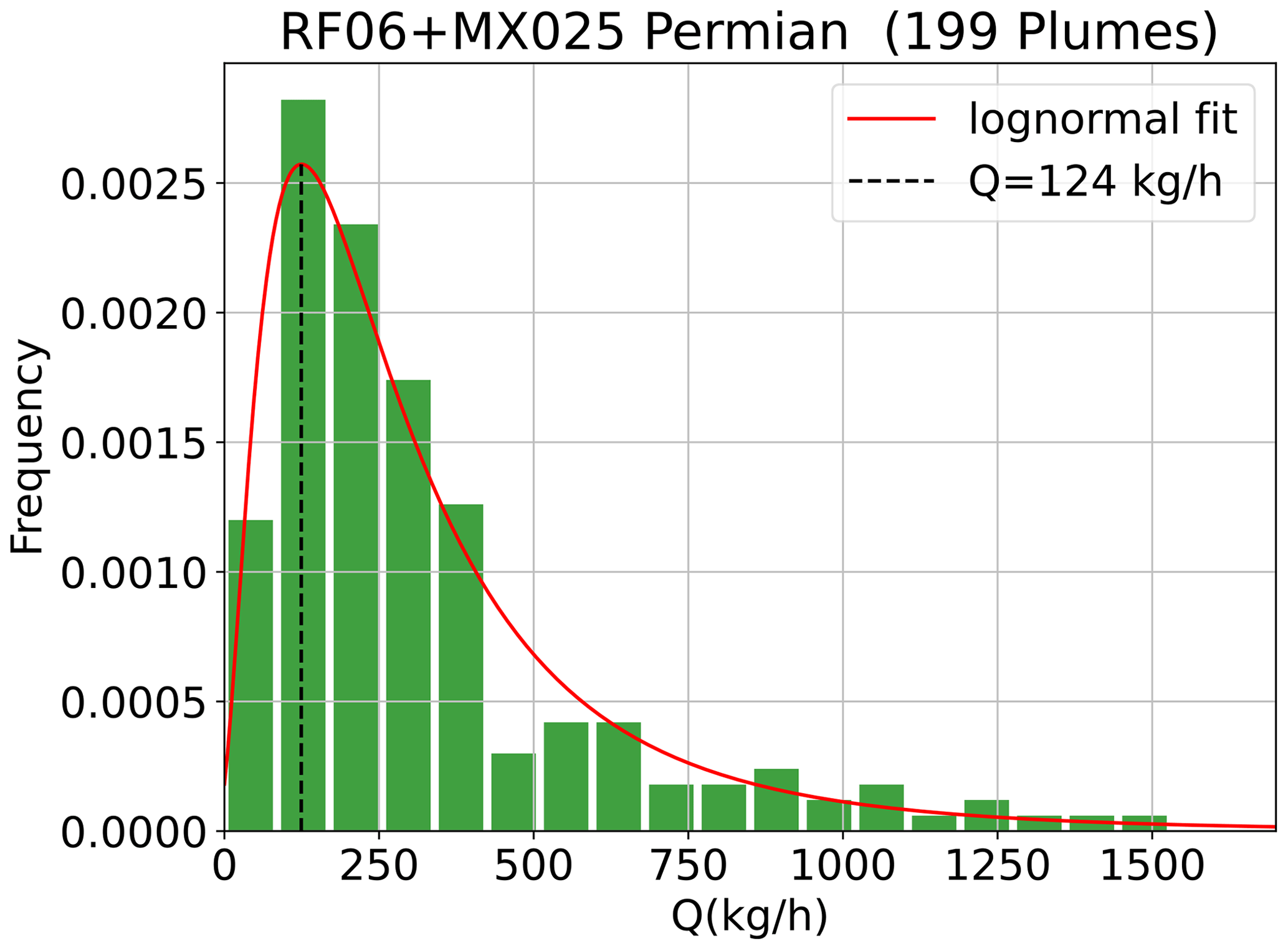
Figure 13 Histogram of the flux rates (Q) estimated from the plumes detected in the RF06 and MX025 datasets. The two campaigns have been combined in order to increase the plume sample. The dash line marks the Q value for which the distribution of estimated Q values deviate from a power law, which can be interpreted as a rough estimation of the source detection limit obtained for MethaneAIR data over the Permian Basin using the processing scheme proposed in this work.

4 Conclusions

We have developed a processing chain for the detection and quantification of point source methane emissions with the MethaneAIR airborne spectrometer. Our goal was to implement a ΔXCH₄ retrieval that was both computationally efficient and able to maximize the probability of plume detection. We have achieved those goals by combining a data-driven ΔXCH₄ retrieval, based on the matched-filter concept, with a plume detection and segmentation approach, based on visual inspection of the resulting ΔXCH₄ maps. Flux rates are estimated from the detected plumes using an IME-based method. This processing scheme enabled the analysis of methane point sources across the Permian Basin using data from two campaigns in 2021 and 2023.

We have shown the potential of the matched-filter retrieval for high-spectral-resolution measurements in the 1650 nm window. The results from our matched-filter ΔXCH₄ retrieval compare well with those from the physically based CO₂-proxy XCH₄ retrieval used in MethaneAIR's operational processing chain. The matched-filter retrieval can only provide XCH₄ enhancements; therefore, it is not an alternative to the CO₂-proxy XCH₄ retrieval, which does provide the total XCH₄ column content required to evaluate area emissions. However, the ΔXCH₄ retrieval by the matched-filter is simple to implement and computationally efficient; moreover, it offers a lower retrieval noise than the CO₂-proxy XCH₄ retrieval, which is advantageous for point source work.

Our results from the processing and analysis of two MethaneAIR flights over the Permian Basin show the potential of MethaneAIR with respect to the detection and quantification of methane point sources across large areas, with about 120 plumes being detected during the 2021 flight and about 80 being detected during the 2023 flight, resulting in a combined detection limit for which most of the plumes would be detected of about 124 kg h⁻¹. We attribute part of the differences in the number of plumes detected from each flight to changes in oil and gas production in the region over time, although different data acquisition conditions between the two campaigns may also have impacted the plume detection limits. In particular, the stronger winds found in 2023, compared with those in 2021, may have led to the greater detection limits, which is also consistent with the findings by other authors (Ayasse et al., 2023).

We have opted for a manual plume detection and segmentation approach in order to ensure that the maximum number of plumes could be detected, with a minimum rate of false positives. However, this step introduces the need for a human in the loop in our processing chain, which challenges its application to large volumes of data, despite the improvement in processing time enabled by the matched filter. Machine-learning-based plume detection approaches (e.g. Růžička et al., 2023) could help reduce the need for human supervision, although the implementation of a fully automated processing chain is challenging if both the detection limits and the probability of false positives are to be kept to a minimum, as was the goal in this work.

Overall, the computationally efficient approach described here as applied to MethaneAIR measurements can also be extended to MethaneSAT in order to help advance the point source detection capacity, as the spectral characteristics are very similar between the airborne and satellite instruments.