Machine learning data fusion for high spatio-temporal resolution PM_2.5

Understanding PM_2.5 variability at fine scale is crucial to assess urban pollution impact on the population and to inform the policy-making process. PM_2.5 in-situ measurements at ground level cannot offer gapless spatial coverage, while current satellite retrievals generally cannot offer both high-spatial and high-temporal resolution, with night-time estimation posing further challenges. This study tackles these difficulties, introducing an innovative deep learning data fusion method to estimate hourly PM_2.5 maps using a grid with cell size 100 m × 100 m on urban areas. We combine low resolution geophysical model data, high resolution geographical indicators, PM_2.5 in-situ ground stations measurements and PM_2.5 retrieved at satellite overpass. To simultaneously treat spatial and temporal correlations in our data, we deploy a 3D U-Net based neural network model. To evaluate the model, we select the city of Paris, France, in the year 2019 as our study region and time. Quantitative assessment of the model is carried out using the ground station data with a leave-one-out cross-validation approach. Our method outperforms MERRA-2 PM_2.5 estimates, predicting PM_2.5 hourly (R² = 0.51, RMSE = 6.58 µg m⁻³), daily (R² = 0.65, RMSE = 4.92 µg m⁻³), and monthly (R² = 0.87, RMSE = 2.87 µg m⁻³). The proposed approach and its possible future developments can be highly beneficial for PM_2.5 exposure and regulation studies at fine suburban scale.

1 Introduction

One of the key indicators in air quality monitoring and regulation is PM_2.5 which is the concentration of particulate matter (PM) with an aerodynamic diameter less than 2.5 µm in cubic meter of air (µg m⁻³). PM_2.5 has different chemical compositions and its emissions originate from different natural and anthropogenic sources such as fuel combustion, wildfires, and sea salt. From the epidemiological point of view, high PM_2.5 levels have been connected to many illnesses, such as stroke and cardiovascular and respiratory diseases (Pope and Dockery, 2006; Cohen et al., 2017; Thangavel et al., 2022). The pathogenicity of fine particulate matter pollution makes it one of the biggest environmental health risks as over 90 % of the world's population lives in areas with annual mean PM_2.5 levels exceeding the new WHO 2021 air quality guideline of 5 µg m⁻³ (Health Effects Institute, 2019).

PM_2.5 and other pollutants can be measured with high accuracy by in-situ ground station networks. However, the existing monitoring sites are sparsely located and mostly in developed countries, typically few stations in a large metropolitan area producing accurate measurements representing the conditions in the proximity of the ground stations. Despite some spatial interpolation techniques could be used (Deng, 2015; Koo et al., 2024) to estimate PM_2.5 over larger urban areas from the point-like measurements obtained by these ground stations, they do not alone permit accurate spatially distributed estimates for epidemiological studies and regulation at a suburban level scale. Aiming at a more appropriate spatial coverage and resolution, PM_2.5 can also be estimated by using airborne remote-sensing techniques, in particular satellite retrievals. In satellite remote sensing, PM_2.5 estimates are typically based on Aerosol Optical Depth (AOD), a quantity expressing electromagnetic radiation extinction through a column of air at a given wavelength. AOD is a columnar optical quantity while PM_2.5 is a concentration of particles at ground level. For AOD to PM_2.5 conversion, the estimation utilizes auxiliary measurement and model data such as aerosol vertical distribution and metereological variables (Chu et al., 2016; Tang et al., 2024). Nowadays many AOD satellite products exist with different spatial and temporal resolution. Different studies used low orbiting satellites (e.g. MODIS product; Levy et al., 2013) that have one or two overpasses per day or geostationary satellites (e.g. AHI product; Bessho et al., 2016) giving sub-hourly estimates. Instruments on low orbiting satellites have generally higher spatial resolution than geostationary ones. Although giving high spatial resolution PM_2.5 estimates, low orbiting satellites products have low temporal resolution (1–2 snapshots per day) and retrieving information on night-time aerosols is a challenging task for the development of geostationary satellites products. Reanalysis models such as MERRA-2 (Randles et al., 2017) and CAMS (Inness et al., 2019), and forecast models such as GEOS-CF (Keller et al., 2021) offer hourly PM_2.5 available globally. However, the spatial resolution of these PM_2.5 maps is low (tens of kilometers) for higher resolution studies such as distribution of pollution at suburban levels.

In recent years, numerous machine learning approaches have been investigated and shown to be effective for air quality monitoring and PM_2.5 forecasting. Several deep learning models leverage both spatial and temporal dependencies in meteorological and aerosol data to enhance prediction performance. For instance, a study conducted across the Greater Los Angeles area employed Graph Convolutional Networks (GCNs) and Convolutional Long Short-Term Memory (ConvLSTM) models to integrate satellite remote sensing data with ground-based monitoring, enabling accurate prediction of PM_2.5 concentrations (Muthukumar et al., 2022). Another study focused on the Seoul region combined air quality and meteorological data using kriging interpolation and a hybrid ConvLSTM-DNN model to generate PM_2.5 concentration maps (Koo et al., 2024).

To estimate PM_2.5, we recently proposed a method (Porcheddu et al., 2024) leveraging the Sentinel-3 POPCORN AOD product (Lipponen et al., 2022). The POPCORN AOD is a post-process corrected version of Sentinel-3 SYNERGY land AOD, characterized by a high spatial resolution on a grid with cell size 300 m × 300 m and derived using a feed-forward neural network trained on AERONET-collocated data. This enhanced AOD product provides accurate spectral aerosol information for five regions of interest (Central Europe, Eastern USA, Western USA, Southern Africa, and India) for the year 2019, making it a valuable input for air quality estimation models. To post-process correct the MERRA-2 AOD-to-PM_2.5 conversion ratio, we deployed an ensemble of deep neural networks for a fusion of collocated ground station in-situ PM_2.5 data, MERRA-2 reanalysis model AOD and PM_2.5 data, spectral AERONET AOD, satellite-observed spectral top-of-atmosphere reflectances, and meteorology data. We also used various high-resolution geographical indicators representing, e.g., population density and land surface elevation. The deep learning model was used for estimation of PM_2.5 on a grid with cell size 100 m × 100 m from low orbiting satellite images, producing 1–2 daily per overpass snapshots of high-resolution PM_2.5 data where AOD data was available.

In this study, we have two research questions. How could we obtain PM_2.5 maps offering large (e.g. metropolitan level) spatial coverage with both high spatial and temporal resolution? Considering satellite derived PM_2.5 maps where AOD data is missing, e.g. because of cloud covering, how can we estimate PM_2.5 at those locations? To address these questions, we propose a novel deep learning based data fusion method to produce hourly PM_2.5 estimates on a grid with cell size 100 m × 100 m. We use a 3D U-Net architecture (Çiçek et al., 2016) to produce 24 h sequences of hourly PM_2.5 maps. The model is trained to yield a small L₂-misfit with the PM_2.5 estimates obtained during satellite overpasses in our previous study (Porcheddu et al., 2024), as well as with available ground station data. As inputs, we utilize 24 h sequences of geophysical model data (MERRA-2) providing low-resolution maps of meteorological and aerosol-related indicators (1 h temporal resolution), and high-resolution geographical indicator maps (1-month temporal resolution). This allows the model to generate hourly PM_2.5 outputs for the entire 24 h period covered by the inputs. The model is trained on data for the year 2019 in the city of Paris, France, and assessed against ground station data with a leave one out cross validation approach.

2 Data

This section describes the data used in the proposed deep learning based data fusion for high resolution PM_2.5. The proposed approach is tested using data from Paris, France, for the year 2019. NOODLESALAD PM_2.5 and OpenAQ PM_2.5 data are used as target to train and test our model. MERRA-2 data and high-resolution geographical indicators are utilized as input features. Since our satellite-based target variable (NOODLESALAD PM_2.5) is represented on a grid with cell size 100 m × 100 m, we train the model on the same grid, considering that some input features are on coarser and others on finer spatial representations. With this approach the model represents spatial patterns at the target data scale when fusing information from input data with different spatial scales. All the input features are listed in Table A1 in the Appendix. It is important to notice that other similar data sources could be utilized with our methodology.

2.1 NOODLESALAD PM_2.5

NOODLESALAD PM_2.5 (Porcheddu et al., 2024) retrievals are obtained applying a deep learning based post-process correction approach to the MERRA-2 AOD-to-PM_2.5 conversion ratio. The post-process corrected AOD-to-PM_2.5 conversion ratio is utilized to map high resolution POPCORN SENTINEL-3 SYNERGY AOD estimate (Lipponen et al., 2022) to high resolution PM_2.5 estimate. The post-process correction of MERRA-2 AOD-to-PM_2.5 conversion ratio is carried out deploying an ensemble of fully-connected feed-forward neural networks and a fusion of surface in-situ PM_2.5 observations, MERRA-2 reanalysis model AOD and PM_2.5 data, spectral AERONET AOD, satellite-observed spectral top-of-atmosphere reflectances, meteorology data, and various high-resolution geographical indicators. The ensemble technique leads to a distribution of predictions for a single PM_2.5 estimate. The median of the ensemble is considered as the PM_2.5 estimate and the width of the distribution is regarded as an uncertainty related to the machine learning model training (model uncertainty). NOODLESALAD PM_2.5 offers high resolution on a grid with cell size 100 m × 100 m and is currently available for Sentinel-3A and 3B overpasses, covering Central Europe for the year 2019. The two Sentinel-3 satellites currently flying provide revisit times of less than two days for OLCI and less than one day for the SLSTR instrument at equator. Swath width of the OLCI instrument is 1270 km. SLSTR swath width is 1420 km for the nadir view and 750 km for the oblique view.

Evaluation metrics for PM_2.5 at satellite overpass (R²=0.55, RMSE = 6.2 µg m⁻³) and PM_2.5 monthly averages (R²=0.72, RMSE = 3.7 µg m⁻³) show good agreement between NOODLESALAD PM_2.5 and OpenAQ ground stations data (Porcheddu et al., 2024). Given the better spatial coverage compared to ground stations and the high spatial resolution at satellite overpass, we utilize NOODLESALAD PM_2.5 to inform the model about PM_2.5 fine spatial distribution. In this work, we consider NOODLESALAD PM_2.5 retrievals in Paris, France, in 2019, and utilize them as part of the target data to train our model.

2.2 OpenAQ

OpenAQ (https://openaq.org/, last access: 13 April 2023) is an open-access database for ground stations air quality data. In this study, we utilize OpenAQ as our source for surface in-situ PM_2.5 observations. OpenAQ offers pointwise air quality measurement data from thousands of stations. The temporal resolution of the data varies by station, with 1 h and daily observations commonly available. Figure 1 shows a map of OpenAQ stations that provide hourly data within our region of interest. We discard PM_2.5 observations when they are greater than the calculated upper fence $Q\mathrm{3}+\mathrm{6}\times (Q\mathrm{3}-Q\mathrm{1})$ (where Q3 and Q1 are respectively the third and first quartiles of the PM_2.5 distribution), regarding them as outliers. This step was carried out to filter extreme outliers, which can be caused by exceptional events or ground station malfunctions.

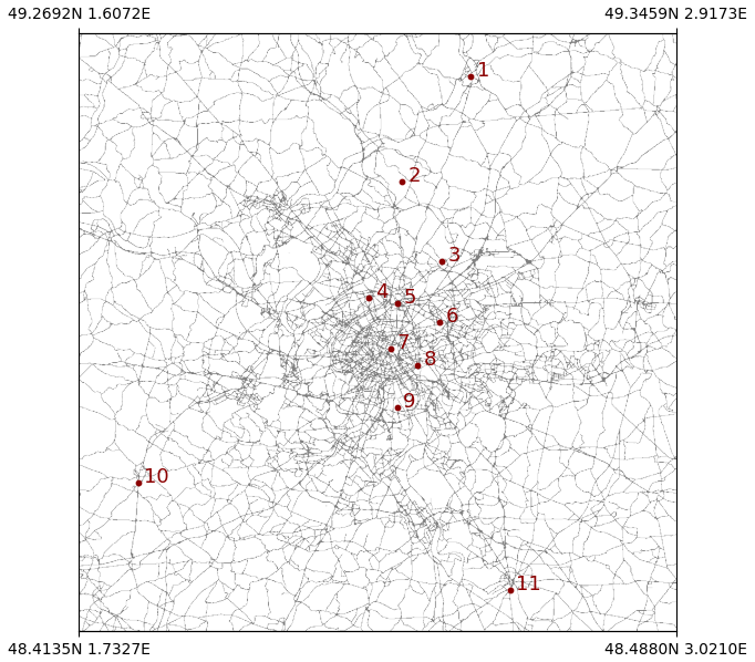
Figure 1 Map of OpenAQ stations in the region of interest (Paris, France).

2.3 MERRA-2

The Modern-Era Retrospective analysis for Research and Applications, Version 2 (MERRA-2), is NASA's reanalysis model (Randles et al., 2017). MERRA-2 provides model data for various variables in meteorology, aerosols and air quality. MERRA-2 has a spatial resolution of 0.5° × 0.625°, which is approximately 50 km in the Central Europe region. The time-varying variables from MERRA-2 that we use have a temporal resolution of 1 h, with both instantaneous and time-averaged values available depending on the variable and data product. Appendix A contains a list of all MERRA-2 variables that are used as inputs in the proposed approach.

In addition to the variables contained in the MERRA-2 data, we calculate certain input variables from the MERRA-2 meteorological and aerosol data. These data are defined as:

• Relative humidity (RH) at the surface. Equation based on the Clausius-Clapeyron equation (see e.g. Michaelides et al., 2019):

  $$\begin{array}{}\text{(1)}& \begin{array}{rl}\mathrm{RH}=& \mathrm{0.263}\cdot \mathrm{PS}\cdot \mathrm{QLML}/\exp \left(\right(\mathrm{17.67}\\ & \cdot (\mathrm{T}\mathrm{2}\mathrm{M}-\mathrm{273.15}))/(\mathrm{T}\mathrm{2}\mathrm{M}-\mathrm{29.65}\left)\right)\end{array}\end{array}$$

• Wind direction (WD10M) at 10 m:

  $$\begin{array}{}\text{(2)}& \mathrm{WD}\mathrm{10}\mathrm{M}=\arctan \left(-\mathrm{V}\mathrm{10}\mathrm{M}/\mathrm{U}\mathrm{10}\mathrm{M}\right)\end{array}$$

• Wind speed (WS10M) at 10 m:

  $$\begin{array}{}\text{(3)}& \mathrm{WS}\mathrm{10}\mathrm{M}=\sqrt{\mathrm{U}\mathrm{10}{\mathrm{M}}^{\mathrm{2}}+\mathrm{V}\mathrm{10}{\mathrm{M}}^{\mathrm{2}}}\end{array}$$

• PM_2.5 at surface: (Buchard et al., 2016)

  $$\begin{array}{}\text{(4)}& \begin{array}{rl}{\mathrm{PM}}_{\mathrm{2.5}}=& (\mathrm{1.375}\cdot \mathrm{SO}\mathrm{4}\mathrm{SMASS}+\mathrm{1.4}\cdot \mathrm{OCSMASS}\\ & +\mathrm{BCSMASS}+\mathrm{DUSMASS}\mathrm{25}\\ & +\mathrm{SSSMASS}\mathrm{25})\cdot {\mathrm{10}}^{\mathrm{9}}\end{array}\end{array}$$

• AOD-to-PM_2.5 ratio η:

  $$\begin{array}{}\text{(5)}& \mathit{\eta }={\displaystyle \frac{{\mathrm{PM}}_{\mathrm{2.5}}}{\mathrm{TOTEXTTAU}}}\end{array}$$

2.4 High-resolution geographical indicators

All geographic variables with the original resolution larger than 100 m were regridded to a common spatial grid with a resolution of 100 m using the Universal Transverse Mercator (UTM) projection. Linear interpolation method was used for continuous features and nearest neighbor interpolation for categorical variables. This preprocessing ensured that all features were spatially collocated prior to input into the deep learning model.

2.4.1 OpenStreetMap roads

OpenStreetMap is an open-source project that contains high spatial resolution map data. In our model, we utilize OpenStreetMap roads as a data source for inputs. Specifically, we calculate the distance to the nearest street or highway and use this measurement as one of our input variables. The distances are computed on a grid with cell size 100 m × 100 m. In OpenStreetMap, all paths, streets, and highways are categorized under “highways”. However, we only consider certain sub-classes that include roads and highways accessible to car traffic, as these are potential sources of PM_2.5 pollution (information from OpenStreetMap, 2023). Appendix A lists all the OpenStreetMap road types used to determine the distance to the nearest road.

2.4.2 NASA Black Marble Night Lights

NASA's Black Marble is a night light product derived from the Visible Infrared Imaging Radiometer Suite (VIIRS) day/night band (DNB) radiances captured during night-time. The DNB is extremely sensitive to light, allowing it to detect even very low-intensity lights on Earth's surface at night. Most of these night-time lights are attributed to human activities. Since the distribution of night lights closely reflects human presence, we use NASA's Black Marble Night Lights as a proxy for population density, incorporating it as an input in our models. We utilize Night Light data with a spatial resolution of 500 m, based on the annual data product VNP46A4 (Wang et al., 2020).

2.4.3 MODIS land cover type

We utilize the MODIS MCD12Q1 land cover type data product (Sulla-Menashe and Friedl, 2018) to generate input variables that represent the distances to the nearest International Geosphere Biosphere Programme (IGBP) land cover types (Loveland and Belward, 1997; Belward et al., 1999). The MODIS MCD12Q1 data product has a spatial resolution of 500 m. A complete list of the IGBP land cover types can be found in Appendix A.

2.4.4 Digital elevation model

We utilize the Advanced Spaceborne Thermal Emission and Reflection Radiometer (ASTER) digital elevation model (DEM) to represent land surface elevation (Fujisada et al., 2011, 2012; NASA/METI/AIST/Japan Spacesystems and US/Japan ASTER Science Team, 2019). The ASTER DEM provides a spatial resolution of 1 arcsecond, which is approximately 30 m.

3 Methods

Our objective is to estimate time series of surface PM_2.5 maps (3D PM_2.5 arrays, two spatial dimensions and one time dimension) in the region of interest by fusion of satellite and ground station measurement data, model data and different indicators as inputs for the deep learning model. Since we are dealing with unstructured data in the form of images, a well-suited choice for the machine learning model is a Convolutional Neural Network (CNN) (LeCun et al., 1989; Bishop and Bishop, 2024). Furthermore, since both the input maps and the output maps represent the same region of interest, a U-Net model is an appropriate choice (Ronneberger et al., 2015). As the data is in 3D, we choose a variant of U-Net called 3D U-Net (Çiçek et al., 2016). The main difference between conventional U-Net and 3D U-Net is that the latter deploys 3D convolutions instead of 2D convolutions for processing 3D image data.

One must note that other network architectures could also be utilized. One possibility would be, e.g., to use a U-Net with convolutional Long Short-Term Memory (LSTM) layers (Shi et al., 2015). Convolutional LSTM layers behave as LSTM layers, with the key difference of performing their internal operations as convolutions, consequently being a possible choice for processing time series of 2D images. Nevertheless, we decided to use 3D U-Net as it was found computationally feasible and less memory intensive for processing the large data sets.

The input data consist of 4 dimensional arrays. The first dimension represents time and has size 24 in order to contain hourly information of a single day. The second dimension contains the different channels (i.e. the different input features) and the remaining two dimensions are the spatial dimensions with image size of 960 × 960. The output is a 3 dimensional array containing 24 hourly PM_2.5 maps in the region of interest as 960 × 960 images with pixel size 100 m × 100 m.

Figure 2 Visualization of the applied neural network architecture.

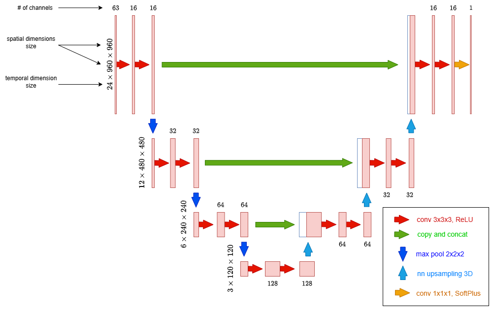
The model architecture has been implemented using the PyTorch framework (Paszke et al., 2019), a widely used library known for its flexibility and efficiency in developing deep learning models. A detailed schematic of the model architecture is provided in Fig. 2 to illustrate its structure and components, whereas Fig. 3 visualizes the corresponding data flow.

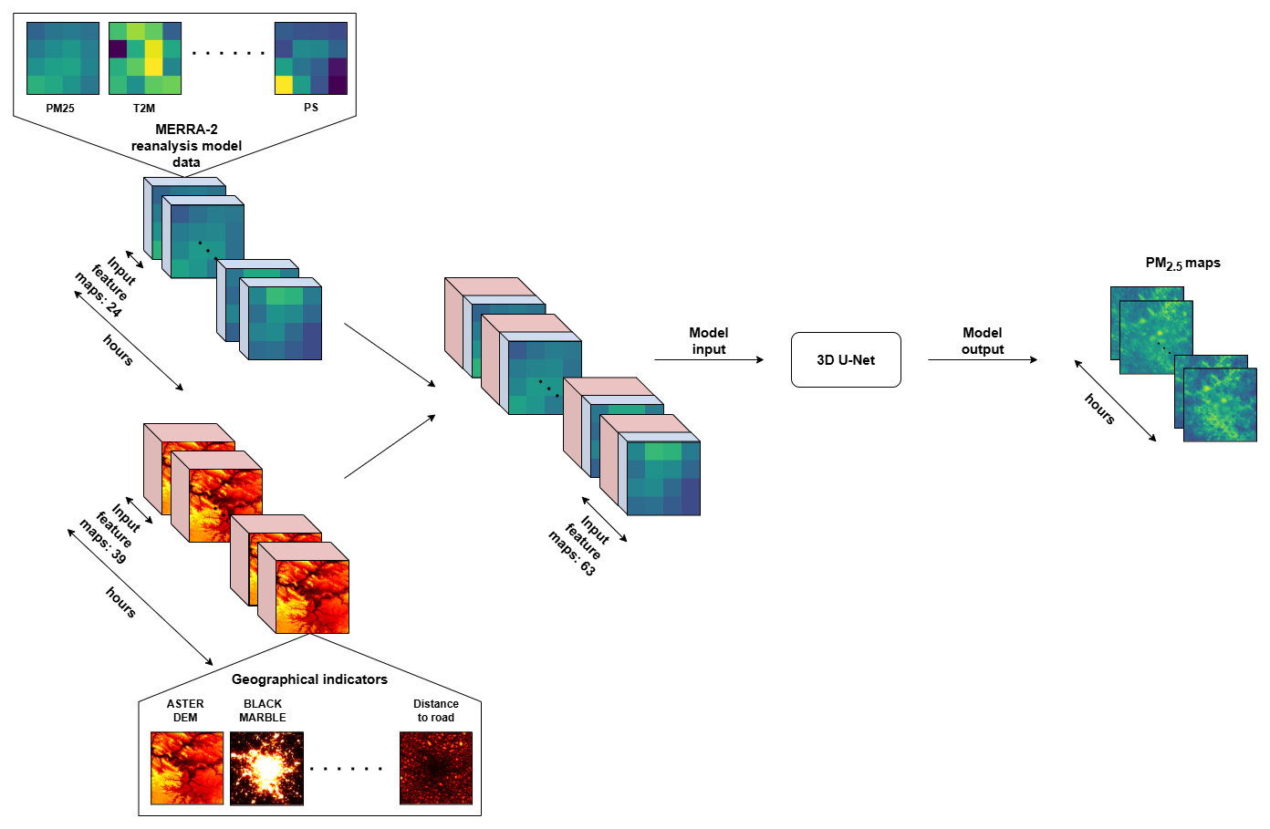
Figure 3 Visualization of the data flow in our method. Low spatial resolution (MERRA-2) data and high spatial resolution geographical indicators are projected on a common grid, joined and utilized as model input. The model output consists of hourly PM_2.5 maps.

The model consists of a contracting path (the encoder) and an expansive path (the decoder). On each level of the contracting path, 3D convolutions combined with ReLU activations and max pooling layers help in finding relevant features from the input maps, producing a new representation of the input with lower spatial and temporal resolution with a higher number of channels. The expansive path deploys 3D nearest neighbour upsampling and 3D convolutions followed by ReLU activations in order to recover a final output with the same spatial and temporal resolution of the input. Notice the skip connections linking each contracting path level to the corresponding expansive path level: from an intuitive point of view, these are useful to exploit the fine details contained in the input when generating the output. Finally, the output layer is a 3D 1 × 1 × 1 convolution followed by SoftPlus activations in order to constrain the output to be a positive definite array. Please notice that when we talk about 3 × 3 × 3 convolution and 1 × 1 × 1 convolution, we are referring to the size of the convolution kernel/filter along the depth, height, and width of the input volume. The number of parameters involved in the convolution operation can be obtained considering the number of input and output channels at a specific convolution layer (Fig. 2). When testing the network architecture, various kernel sizes, internal activation functions, and upsampling techniques were evaluated, but no significant differences in performance were observed.

3.1 Loss function

We use the Mean Square Error (MSE) as the loss function in the supervised regression problem of fitting the 3D U-Net model to the training data. Ideally in clear sky conditions for a satellite overpass, we would have a full PM_2.5 map. In ideal conditions for a single ground station, we would have a full time series without missing data. However, in reality satellite overpass data can lack information at some pixels, e.g. cloud covering can hinder AOD retrievals, therefore hindering PM_2.5 estimates, and a ground station can malfunction, leading to missing data in the time-series of the station. Furthermore, on a single day we usually have significantly more PM_2.5 pixel values coming from the satellite overpasses than measured values from the ground stations. The ground stations PM_2.5 data are usually more accurate than satellite estimate data and they are our only data source available hourly. On the other hand, NOODLESALAD PM_2.5 is our data source providing information far from the ground stations at the time of satellite overpasses. Therefore, to take the missing data and highly different number of satellite versus ground station data available into account, we consider masking and weighting the data in the MSE loss function.

Let the batch size be denoted by B (with B=4 for this particular case) and define $N=\mathit{\{}\mathrm{1},\mathrm{\dots },\mathrm{960}\times \mathrm{960}\mathit{\}}$ as the set of all pixel indices. For each sample b in the batch, define $H_{\mathrm{st},b}\subseteq \mathit{\{}\mathrm{1},\mathrm{\dots },\mathrm{24}\mathit{\}}$ as the set of hours during which ground stations measurements are available, and $H_{\mathrm{op},b}\subseteq \mathit{\{}\mathrm{1},\mathrm{\dots },\mathrm{24}\mathit{\}}$ as the corresponding set of hours for satellite overpasses. Let $y_{b,h,i}$ represent the target measurement at sample b, hour h, and pixel index i, with ${\widehat{y}}_{b,h,i}$ denoting the corresponding predicted value by the deep learning model. When a measurement is not available (due to lacking data from a ground monitoring station or failed satellite retrieval due to cloud covering) $y_{b,h,i}$ is encoded as 0, since this value does not naturally occur in the dataset (PM_2.5 is not zero in a realistic setting). On the other hand, ${\widehat{y}}_{b,h,i}$ is always a positive real value by choice, since SoftPlus was chosen as activation function for our model output.

For each sample b and hour h, define:

$$\begin{array}{}\text{(6)}& {\displaystyle }{S}_{\mathrm{st},b,h}=\mathit{\{}i\in N\mid y_{b,h,i}\ne \mathrm{0}\text{ and }h\in H_{\mathrm{st},b}\mathit{\}},\text{(7)}& {\displaystyle }{\stackrel{\mathrm{̃}}{S}}_{\mathrm{op},b,h}=\mathit{\{}i\in N\mid y_{b,h,i}\ne \mathrm{0}\text{ and }h\in H_{\mathrm{op},b}\mathit{\}},\end{array}$$

representing pixel indices where ground station measurements ($S_{\mathrm{st},b,h}$) and satellite overpass measurements (${\stackrel{\mathrm{̃}}{S}}_{\mathrm{op},b,h}$) are available. The sets $S_{\mathrm{st},b,h}$ and $S_{\mathrm{op},b,h}$ are defined separately for the ground stations and satellite overpass data. From the satellite overpass data, we create a subset $S_{\mathrm{op},b,h}\subset {\stackrel{\mathrm{̃}}{S}}_{\mathrm{op},b,h}$ of data with 25 % of size of ${\stackrel{\mathrm{̃}}{S}}_{\mathrm{op},b,h}$ by uniform random sampling of the pixels to be used in the minimization. The random sampling is performed at each training step (for every update of the network parameters) and can be seen as an optimization technique analogue to batch shuffling. This undersampling is beneficial for training on overpass estimates, especially given the substantial pixel count (nearly 1 million when all pixels provide valid measurements at overpass times).

The average losses for the ground stations and overpass contributions are defined by summing over the respective sets of valid hours:

$$\begin{array}{}\text{(8)}& {\displaystyle }{L}_{\mathrm{st},b}=C_{\mathrm{st},b}\sum _{h\in H_{\mathrm{st},b}}{\displaystyle \frac{\mathrm{1}}{\left|S_{\mathrm{st},b,h}\right|}}\sum _{i\in S_{\mathrm{st},b,h}}(y_{b,h,i}-{\widehat{y}}_{b,h,i}{)}^{\mathrm{2}}\text{(9)}& {\displaystyle }{L}_{\mathrm{op},b}=C_{\mathrm{op},b}\sum _{h\in H_{\mathrm{op},b}}{\displaystyle \frac{\mathrm{1}}{\left|S_{\mathrm{op},b,h}\right|}}\sum _{i\in S_{\mathrm{op},b,h}}(y_{b,h,i}-{\widehat{y}}_{b,h,i}{)}^{\mathrm{2}}\end{array}$$

where C_st,b and C_op,b are factors depending on the sizes of the sets H_st,b and H_op,b (defined respectively as $\left|H_{\mathrm{st},b}\right|$ and $\left|H_{\mathrm{op},b}\right|$). If these sets are empty, C_st,b and C_op,b are equal to 0, otherwise they correspond to $\frac{\mathrm{1}}{\left|H_{\mathrm{st},b}\right|}$ and $\frac{\mathrm{1}}{\left|H_{\mathrm{op},b}\right|}$ respectively. Analogously, $\left|S_{\mathrm{st},b,h}\right|$ and $\left|S_{\mathrm{op},b,h}\right|$ represent the sizes of the sets $S_{\mathrm{st},b,h}$ and $S_{\mathrm{op},b,h}$.

We then define the sample-specific loss L_b as:

$$\begin{array}{}\text{(10)}& L_b=\left\{\begin{array}{ll}\frac{L_{\mathrm{st},b}+L_{\mathrm{op},b}}{\mathrm{2}},& \text{if }{L}_{\mathrm{st},b}\ne \mathrm{0}\text{ and }{L}_{\mathrm{op},b}\ne \mathrm{0}\\ L_{\mathrm{st},b},& \text{if }{L}_{\mathrm{op},b}=\mathrm{0}\\ L_{\mathrm{op},b},& \text{if }{L}_{\mathrm{st},b}=\mathrm{0}\end{array}\right.\end{array}$$

Finally, the overall loss for the batch is defined as:

$$\begin{array}{}\text{(11)}& \mathcal{L}={\displaystyle \frac{\mathrm{1}}{B}}\sum _{b=\mathrm{1}}^B{L}_b\end{array}$$

This formalization provides the necessary structure to include both ground station and satellite overpass target data within each batch. A schematic representation of the loss function is presented in Fig. 4.

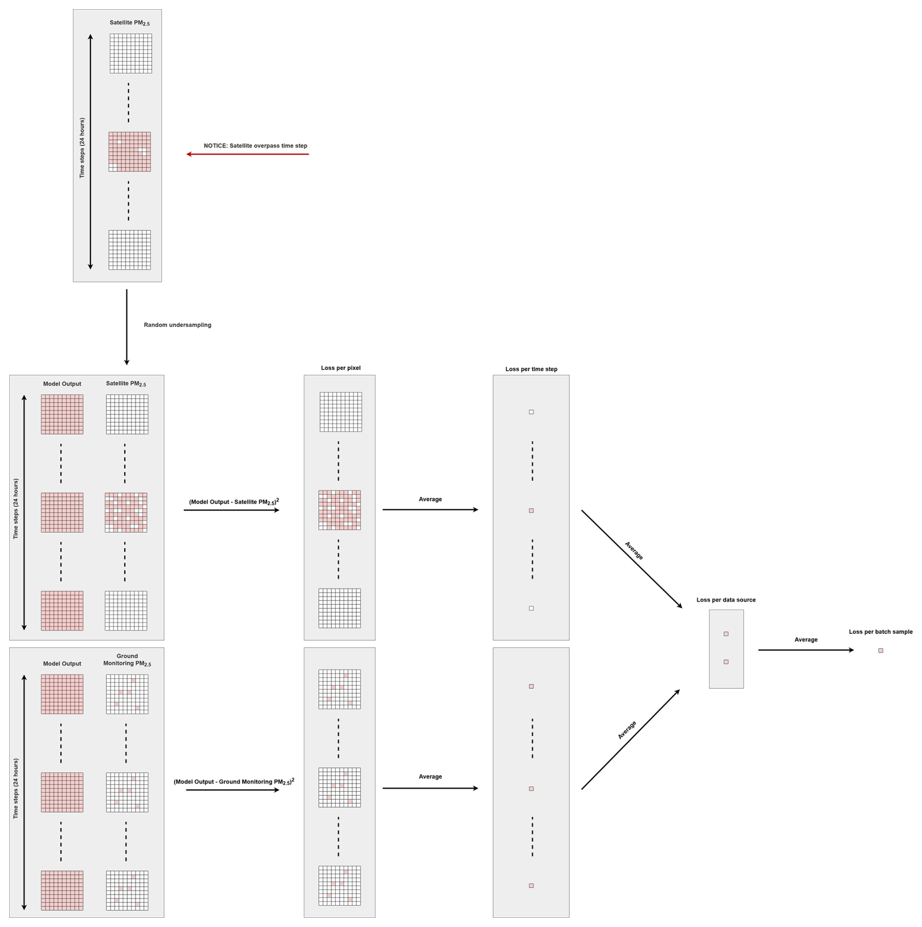
Figure 4 Schematic representation of the loss function. Red squares represent available data points. White squares represent missing data. Black arrows represent operations: these operations are performed using available data (red squares) and the pixels with missing data are omitted.

3.2 Model training

For each data sample, one or two target maps correspond to the available satellite overpasses data (i.e. NOODLESALAD PM_2.5) while the others contain only ground stations data (therefore 11 pixels for each map when data is available from all the stations). In order to test the results from the network training, we used leave-one-out cross-validation (CV) (i.e. we removed one different station from each training and used the data left out of training for testing purposes). Therefore, we trained 11 different networks (one for each ground station in the region of interest). Furthermore, the dataset has been split into training set (approximately 80 % of the data samples) used for the optimization of the network weights and validation set (approximately 20 % of the data samples) used for early stopping of the optimization. The early stopping is a form of regularization useful to avoid overfitting of the network (Goodfellow et al., 2016; Bishop and Bishop, 2024). It consists in keeping track of both the training error and validation error with the objective of stopping the training when the validation error starts to increase (i.e. when the network stops to learn useful patterns and noise in the training set starts to play a significant role). While early stopping is not the only regularization technique applicable to train deep learning models, it offers a good trade-off between model performance and training time. We consider a patience parameter equal to 30, meaning that the training stops when no improvement on the validation loss is recorded over 30 epochs. Since using a small batch size introduces fluctuations in the loss during training, this choice of the patience parameter is reasonable, as a lower patience value could prematurely stop training and lead to underfitting.

We utilized the Adam algorithm (with learning rate equal to 0.0001) and the custom loss function described in Sect. 3.1 to optimize the network model parameters.

4 Results

4.1 Overall performance and evaluation metrics

We considered a leave-one-out CV approach, training 11 models, each time leaving one station out of the training as test station. The results of predicted PM_2.5 at the locations of the 11 AQ stations in Paris are shown in Fig. 5.

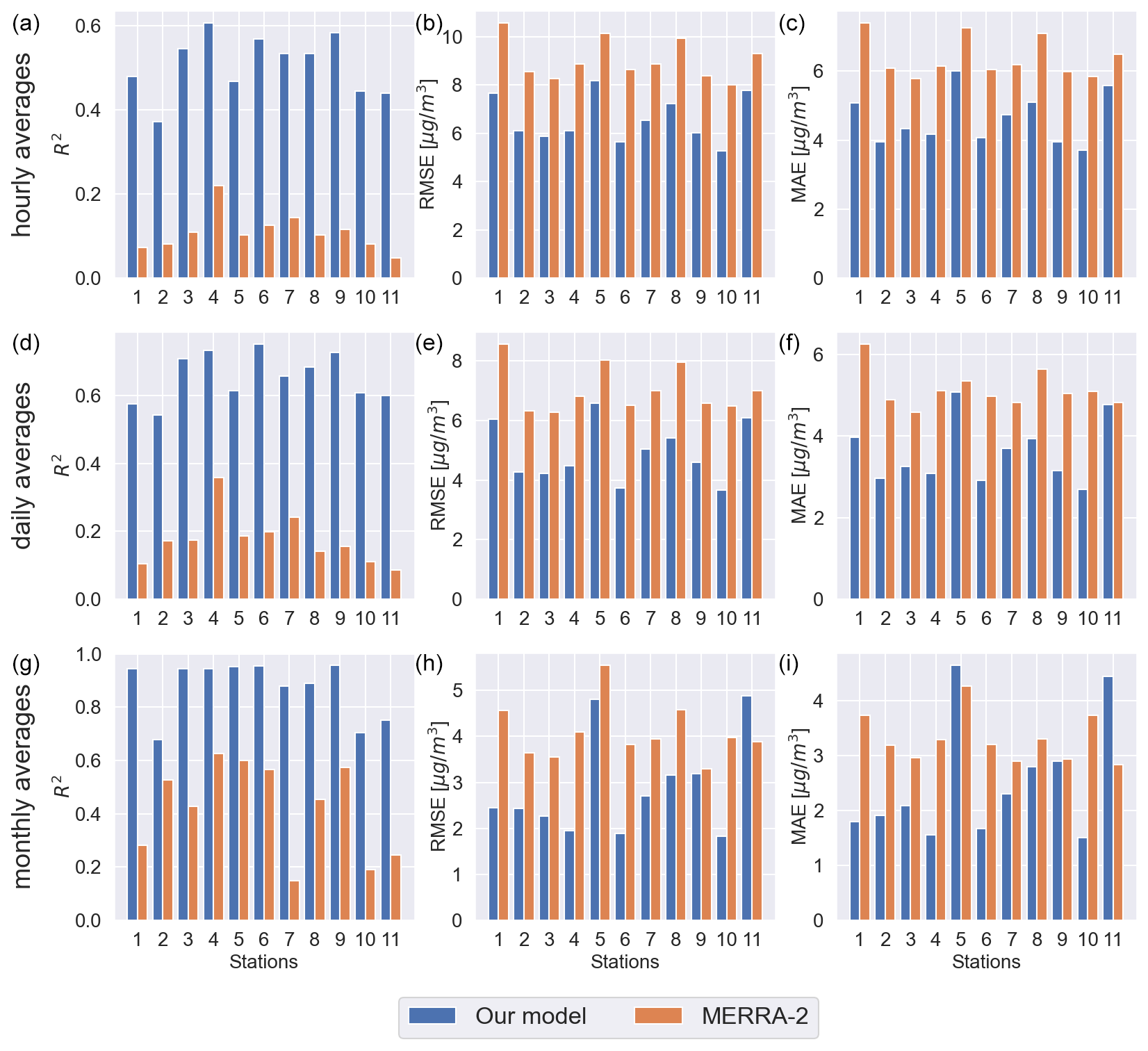
Figure 5 R² (a, d, g), RMSE (b, e, h) and MAE (c, f, i) evaluation metrics resulting from the leave-one-out cross-validation per each test station. The metrics have been calculated for hourly averages (a–c), daily averages (d–f) and monthly averages (g–i). Our model predictions (blue bars) and MERRA-2 estimates (orange bars) are compared to the ground truth data (OpenAQ).

Different fidelity metrics (per each trained model) were calculated to compare MERRA-2 estimates (orange bars) and our model predictions (blue bars) to OpenAQ measurements (ground truth). Correlation R², Root Mean Square Error (RMSE) and Mean Absolute Error (MAE) values are shown on the left, middle and right columns. These metrics are evaluated for hourly averages, daily averages and monthly averages (estimated using the hourly averages) on the top, middle and bottom row. The fidelity metrics averages show that our model clearly outperforms MERRA-2. R² CV averages for our model are 0.51 (hourly averages), 0.65 (daily averages) and 0.87 (monthly averages). R² CV averages for MERRA-2 are respectively 0.10, 0.18, and 0.42. RMSE CV averages for our model are 6.58 µg m⁻³ (hourly averages), 4.92 µg m⁻³ (daily averages) and 2.87 µg m⁻³ (monthly averages). The same metrics averages for MERRA-2 are respectively 9.05, 7.04 and 4.08 µg m⁻³. MAE CV averages for our model are 4.61 µg m⁻³ (hourly averages), 3.59 µg m⁻³ (daily averages) and 2.51 µg m⁻³ (monthly averages). MAE CV averages for MERRA-2 are respectively 6.39, 5.14 and 3.30 µg m⁻³. We can notice from Fig. 5 that our model outperforms MERRA-2 on all hourly and daily value metrics, and in most monthly averaged with the exceptions that MERRA-2 has better monthly MAE for stations 5 and 11, better RMSE for station 11. The R² values still show a clear improvement of our model. For what regards station 5, the better RMSE and worse MAE are due to the fact that RMSE highlights outliers (i.e. MERRA-2 commits less but bigger mistakes). Anyway, the important R² values for both station 5 and station 11 show that our model correctly predicts the AQ trends better but is off mainly by a scaling factor. From Fig. 1, one would expect some differences in the performances at different ground stations, since the more isolated is the station, the less information from surrounding stations is present in the training data (we have ideally full PM_2.5 maps only once per day). Stations 1, 2, 10, and 11 are clearly positioned outside the city center of Paris. Looking at the metrics for these stations, only the location of station 11 seems to have somewhat different prediction accuracy by our model than the stations located in the city center. Although we considered a relatively small dataset to train and test our model, these results suggest it is not overfitting the training data.

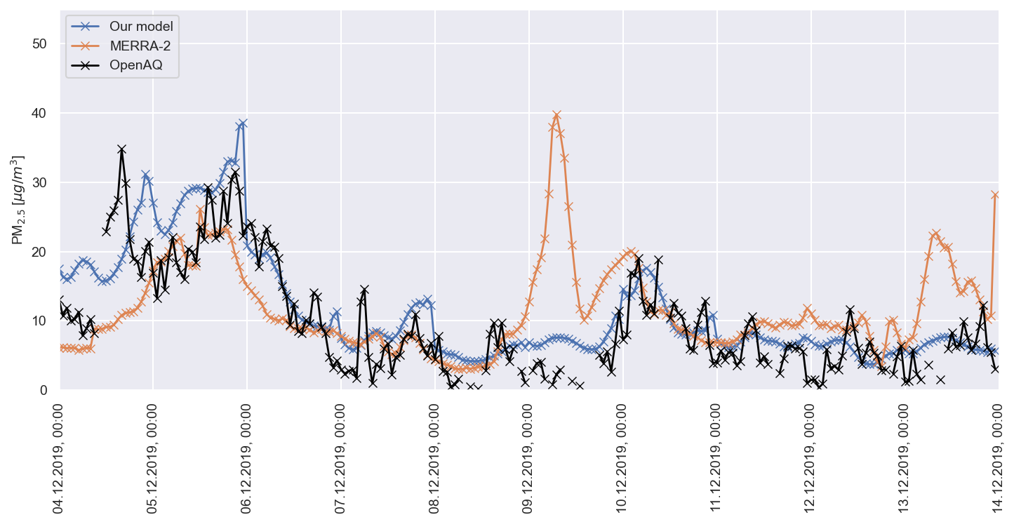
Figure 6 Comparison between hourly PM_2.5 estimates from our model (blue), MERRA-2 (orange) and OpenAQ ground stations measurements (black) at station 1. The period considered runs between 4 and 13 December 2019.

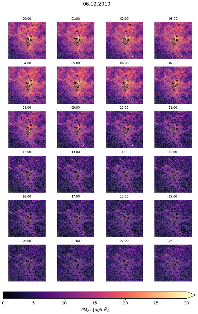
Figure 7 PM_2.5 map on 6 December 2019. The dots reprent PM_2.5 measurements from OpenAQ ground stations.

Figure 6 presents an example of model performance at hourly resolution at Station 1 between 4 and 13 December 2019, compared against MERRA-2 and OpenAQ observations. The comparison illustrates that our model captures the observed variability more accurately than MERRA-2. Figure 7 shows hourly PM_2.5 concentration maps for the Paris region on 6 December 2019, with spatial patterns that agree well with OpenAQ station data. Zooming on these hourly maps we can notice slight block artifacts arising from MERRA-2 input low resolution. This effect could potentially be mitigated via spatial continuity constraints (i.e. adding a regularizer to the loss function) and will be considered in future work.

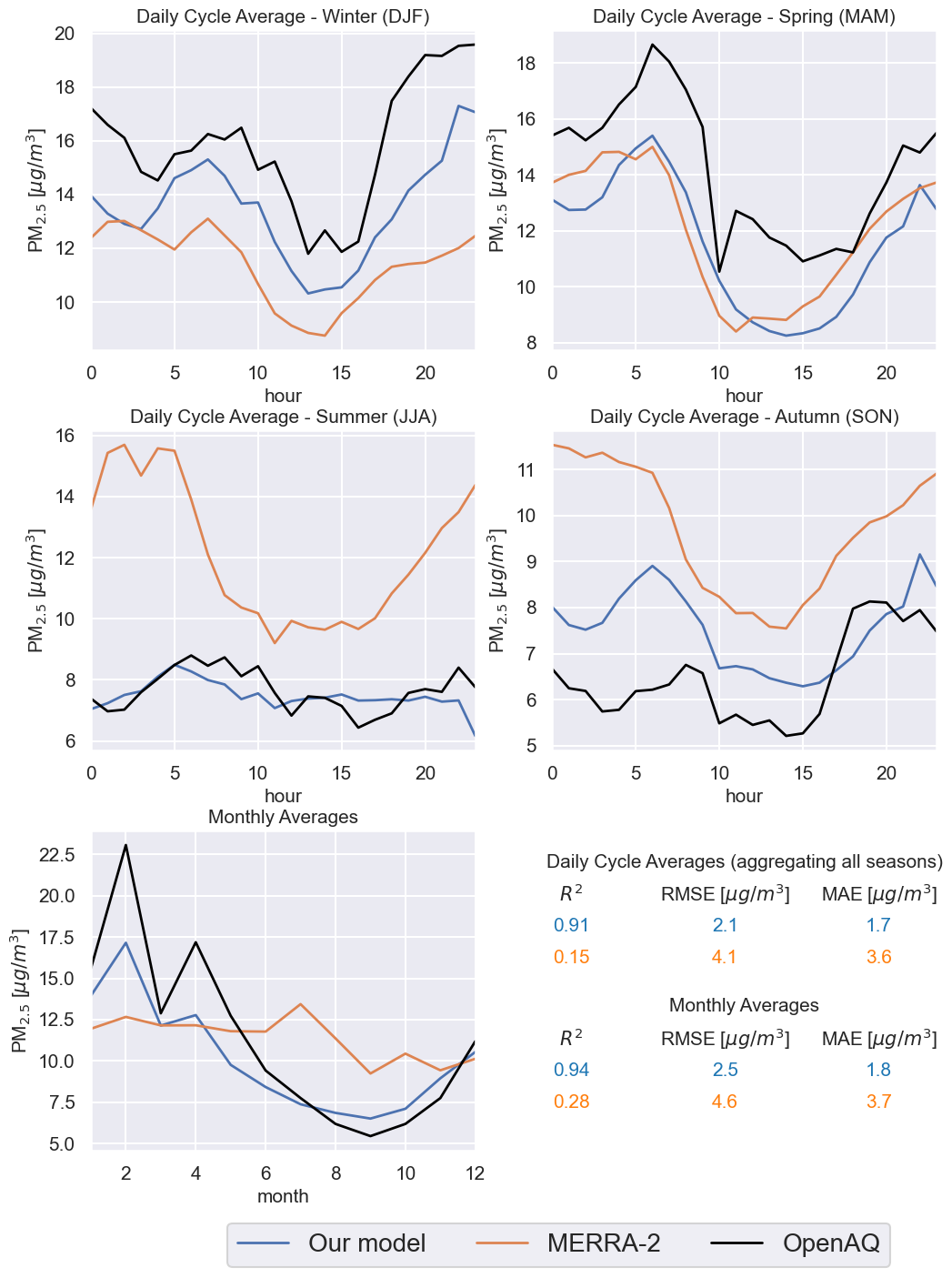
Figure 8 PM_2.5 daily cycle averages for the different seasons and monthly averages (at station 1). The black lines represent OpenAQ measurements, the orange lines represent MERRA-2 estimates and the blue lines are predicted by our model. The evaluation metrics comparing respectively MERRA-2 and our model to the ground truth (OpenAQ) are shown on the bottom-right.

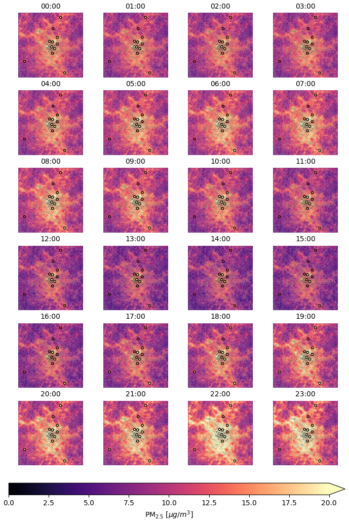
Figure 9 Predicted PM_2.5 seasonal averages maps by hour for the 2019 winter season (December, January and February) on the city of Paris. The dots represent ground stations measurements. These plots are obtained considering the model trained leaving out station 1.

4.2 Seasonal daily trends and monthly averages

Figure 8 shows daily cycle averages on the different seasons (top and middle rows) and monthly averages (bottom row) of 2019 at the test station 1. Black lines represent the ground station measurements, while orange lines and blue lines represent respectively MERRA-2 estimates and our model predictions. Focusing on the daily cycle averages, qualitatively our model and MERRA-2 seem comparable for the spring seasons (March, April, May). The difference is evident on the winter (December, January, February), autumn (September, October, November) and summer (June, July, August) seasons. Especially on the summer season, our model improves notably the accuracy and correlation over MERRA-2. The improvement can be seen quantitatively looking at the metrics on the bottom-right of Fig. 8 (here the estimates for all the seasons have been taken into account in the calculation of the evaluation metrics). Notice how the metrics values for MERRA-2 and our model have been encoded with the same colors of the legend. On the bottom-left of Fig. 8 we compare monthly averages estimates. Again, the difference between MERRA-2 and our model is evident. While MERRA-2 could seem to give a good approximation to the PM_2.5 annual average at the station, it is not able to capture the time series trend. Our model improves notably from this point of view, showing also improvements in accuracy. This is clear from the metrics for monthly averages, where the R² is more than 3 times higher for our model, while the RMSE and MAE are about half of the respective errors in the MERRA-2 estimates.

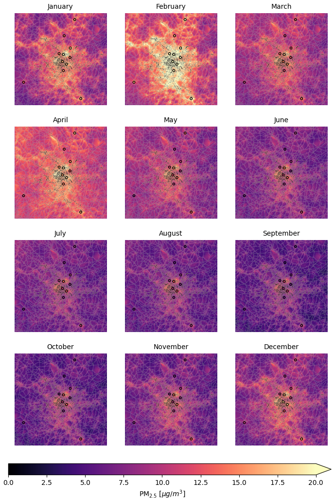
Figure 10 Predicted PM_2.5 monthly averages maps for the year 2019 on the city of Paris. The dots represent ground stations measurements. These plots are obtained considering the model trained leaving out station 1.

Figure 9 shows PM_2.5 seasonal averages maps by hour for the 2019 winter season (December, January, February) predicted by our model on the city of Paris. The dots represent ground stations measurements. The general time series trend reflects the PM_2.5 variations seen in Fig. 8 on the top-left panel. The PM_2.5 levels seem to decrease at day time, and raise again at night time. This behaviour can be expected and physically explained through boundary layer height variations. Spatial variations of PM_2.5 are reasonable and in agreement with what found predicting PM_2.5 levels at satellite overpass (Porcheddu et al., 2024): the city center and areas surrounding main highways are predicted as the most polluted areas. The maps shown in Fig. 9 are obtained considering station 1 as test station.

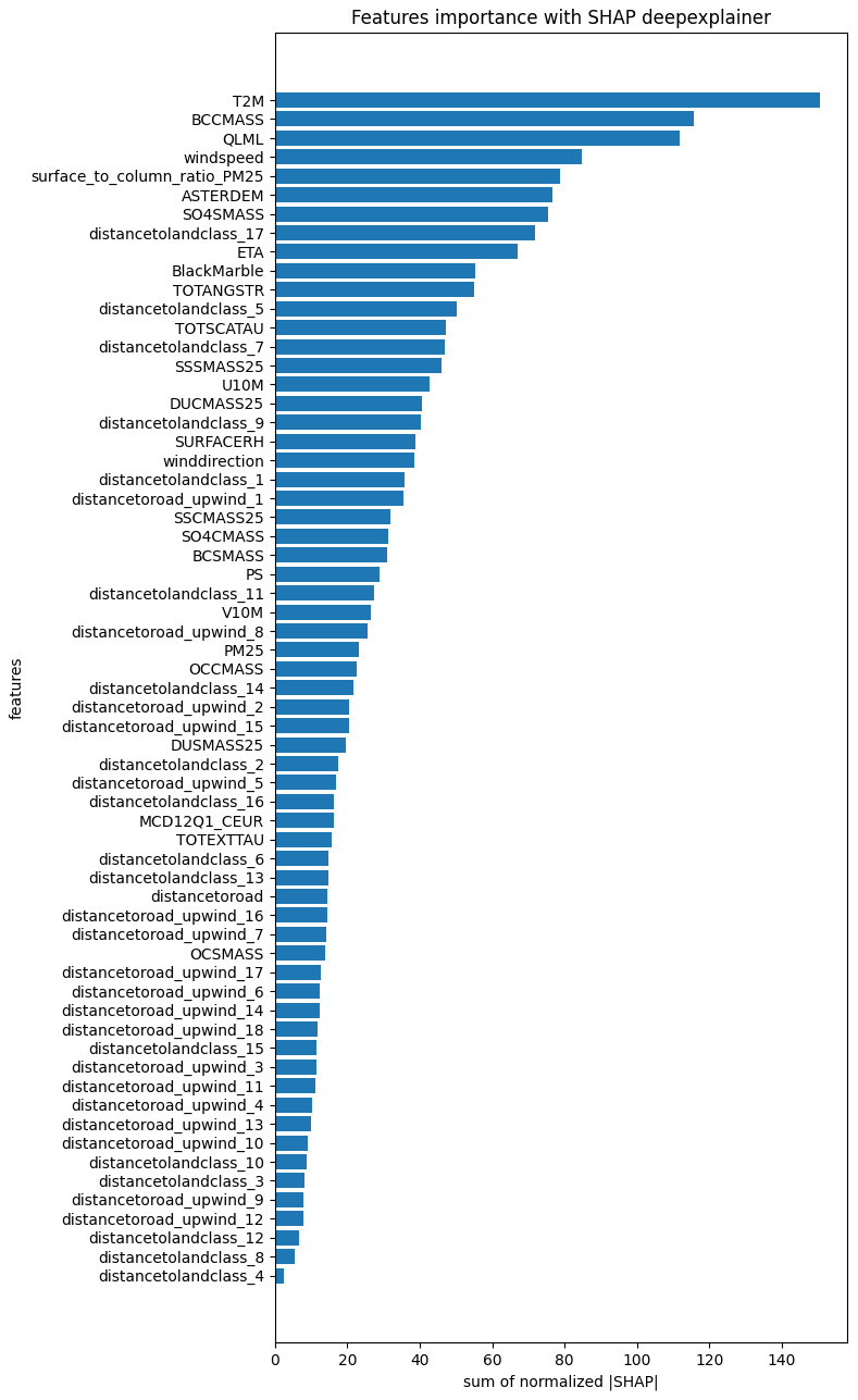
Figure 11 Feature importance calculated as sum of the normalized absolute SHAP values for predictions at station 1.

The maps shown in Fig. 10 represent PM_2.5 monthly averages for the year 2019 predicted by our model on the city of Paris. Dots represent ground stations measurementes. The general time series trend reflects the content of the bottom-left panel in Fig. 8 as expected: PM_2.5 levels are higher in colder months, while lower in warmer months. Again, this temporal variation of PM_2.5 could be explained through boundary layer height variations and also residential heating plays an important role in winter. Spatial variations of PM_2.5 present the same structure already discussed before for Fig. 9. Again, the maps shown in Fig. 10 are obtained considering station 1 as test station. The agreement with the test station and training stations is generally good.

4.3 SHAP explainability

We employed the SHAP DeepExplainer to compute SHAP values and assess feature importance for the model predictions at station 1 (Lundberg and Lee, 2017). Due to computational constraints, the SHAP values were calculated using a smaller background dataset, with analysis conducted on a subset of 90 randomly selected days. Feature importances were determined by summing the normalized absolute SHAP values, and are shown in Fig. 11. As expected, T2M (2 m air temperature) emerged as one of the most significant predictors, consistent with prior findings. For instance, T2M influences the temporal variability of PM_2.5 through boundary layer dynamics and contains information about seasonal emission changes. Specific aerosol variables such as BCCMASS (Black Carbon Column Mass Density), could give the model an idea of how much important black carbon concentration is for the final PM_2.5 estimate, but at the same time act as proxy for other species related to black carbon emission sources. Among the most important high resolution input features, ASTERDEM (ASTER Digital Elevation Model) and BlackMarble (NASA Black Marble Night Lights) offer information about terrain topology and human activities location. While the former could provide useful information about aerosol transport, the latter could act as a proxy for aerosol sources spatial distribution. More generally, aggregating the feature importances in Fig. 11, one can estimate the importance of athmosperic variables (35 %), aerosol variables (25 %) and high resolution indicators (40 %).

5 Conclusions

We developed a novel deep learning data fusion method to estimate hourly PM_2.5 on a grid with cell size 100 m × 100 m, utilizing low-resolution geophysical model data, high-resolution geographical indicators, satellite PM_2.5 retrievals and in-situ PM_2.5 ground measurements. A 3D U-Net based architecture was deployed to take into account both spatial and temporal correlations in the data at hand. The methodology was tested on data from Paris, France, for the year 2019.

The model outperforms MERRA-2 PM_2.5 estimates (our starting point, utilized as model input) on all the evaluation metrics considered. Our estimates are generally consistent with the PM_2.5 spatio-temporal variability assessed by ground stations measurements. Our method seems promising in answering our research questions: reliable gapless PM_2.5 maps at fine scale in absence of AOD data, due to absence of satellite overpass or due to failed AOD retrieval, seem possible.

Further improvements could be obtained by various means. The method is flexible for what concern data sources, as different data sources could be utilized as inputs, and targets in the training process. In particular, different satellite PM_2.5 sources could be considered in the training. So far, we considered only NOODLESALAD PM_2.5. In future studies, we could take into account other satellite data at different satellite overpass times and with different spatial resolution. Considering that geostationary retrievals have high temporal resolution, we could also combine low orbiting instruments and geostationary instruments to integrate all the available information both on the spatial and temporal dimensions. Further, instead of relying solely on data, we could introduce physical constraints in our loss function, pushing the model training to the space of physical solutions assisted by differential equations. Physics Informed Neural Networks (PINNs) (Raissi et al., 2019) have shown promising results in many areas of science and they can be a practical solution to achieve a deep learning based assimilation model at fine scale. It is also important to address the issue of data imbalance. The PM_2.5 distribution in the training data is inherently skewed toward lower values, posing a common challenge in training models. Additionally, satellite retrieval maps (NOODLESALAD PM_2.5) are more susceptible to cloud cover during winter, causing seasonal imbalance to the training data. Expanding the dataset to include more locations and years could help mitigate these issues and improve model performance. We remark that assessment of the credibility of the spatial features in high-resolution air pollution mapping remains an important future topic. However, this is not an straightforward task due to the lack of independent ground based high-resolution data. At scales of single cities, such local data could possibly be obtained from separate measurement campaigns (e.g. using drones) for short time periods or low-cost sensor networks such as PurpleAir which, however, may have somewhat limited accuracy.

In conclusion, given the encouraging results and possible future developments, we believe our methodology could be relevant for PM_2.5 related exposure and regulation studies at finer (suburban level) scale.

Appendix A: Table with input features and lists of variables used from datasets

Table A1 Table of input features for the model.

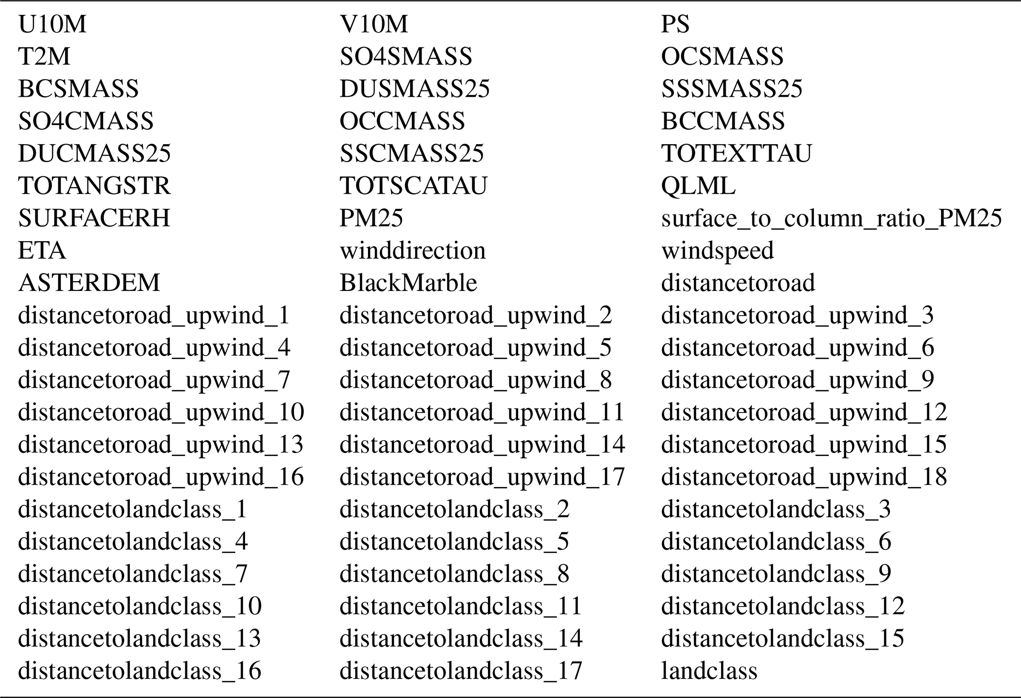
A1 MERRA-2 variables

We use the following meteorology-related variables from the MERRA-2 M2T1NXSLV dataset:

• PS: surface pressure (Pa)

• T2M: 2 m air temperature (K)

• U10M: 10 m eastward wind (m s⁻¹)

• V10M: 10 m northward wind (m s⁻¹)

We use the following meteorology-related variables from the MERRA-2 M2T1NXFLX dataset:

• QLML: surface specific humidity (1)

We use the following aerosol and air quality related variables from the MERRA-2 M2T1NXAER dataset:

• BCCMASS: Black Carbon Column Mass Density (kg m⁻²)

• BCSMASS: Black Carbon Surface Mass Concentration (kg m⁻³)

• DUCMASS25: Dust Column Mass Density – PM_2.5 (kg m⁻²)

• DUSMASS25: Dust Surface Mass Concentration – PM_2.5 (kg m⁻³)

• OCCMASS: Organic Carbon Column Mass Density (kg m⁻²)

• OCSMASS: Organic Carbon Surface Mass Concentration (kg m⁻³)

• SO4CMASS: SO4 Column Mass Density (kg m⁻²)

• SO4SMASS: SO4 Surface Mass Concentration (kg m⁻³)

• SSCMASS25: Sea Salt Column Mass Density – PM_2.5 (kg m⁻²)

• SSSMASS25: Sea Salt Surface Mass Concentration – PM_2.5 (kg m⁻³)

• TOTANGSTR: Total Aerosol Angstrom parameter [470–870 nm] (1)

• TOTEXTTAU: Total Aerosol Extinction AOT [550 nm] (1)

• TOTSCATAU: Total Aerosol Scattering AOT [550 nm] (1)

A2 OpenStreetMap road types used to compute the distance to the closest road

We use the following road types to compute the distance to the closest road. The descriptions of the road types are obtained from OpenStreetMap (2023).

• motorway: A restricted access major divided highway, normally with 2 or more running lanes plus emergency hard shoulder. Equivalent to the Freeway, Autobahn, etc.

• trunk: The most important roads in a country's system that aren't motorways.

• primary: The next most important roads in a country's system.

• secondary: The next most important roads in a country's system.

• tertiary: The next most important roads in a country's system.

• motorway_link: The link roads (sliproads/ramps) leading to/from a motorway from/to a motorway or lower class highway. Normally with the same motorway restrictions.

• trunk_link: The link roads (sliproads/ramps) leading to/from a trunk road from/to a trunk road or lower class highway.

• primary_link: The link roads (sliproads/ramps) leading to/from a primary road from/to a primary road or lower class highway.

• secondary_link: The link roads (sliproads/ramps) leading to/from a secondary road from/to a secondary road or lower class highway.

• tertiary_link: The link roads (sliproads/ramps) leading to/from a tertiary road from/to a tertiary road or lower class highway.

A3 IGBP land cover types

IGBP classification contains the following land cover types:

1. Evergreen needleleaf forests

2. Evergreen broadleaf forests

3. Deciduous needleleaf forests

4. Deciduous broadleaf forests

5. Mixed forests

6. Closed shrublands

7. Open shrublands

8. Woody savannas

9. Savannas

10. Grasslands

11. Permanent wetlands

12. Croplands

13. Urban and built-up

14. Cropland/natural

15. Snow and ice

16. Barren

17. Water bodies