Ship-based lidar measurements for validating ASCAT-derived and ERA5 offshore wind profiles

The accurate characterisation of offshore wind resources is crucial for the efficient planning and design of wind energy projects. However, the scarcity of in situ observations in marine environments requires the exploration of alternative and reliable data sources. In response to this challenge, this study presents a comprehensive comparison between wind profiles derived from the Advanced Scatterometer (ASCAT) satellite observations and the ECMWF Reanalysis fifth-generation (ERA5) dataset against ship-based lidar measurements in the northern Baltic Sea. The aim is to investigate the applicability of ship-based lidar measurements for validating these datasets and to better understand the reliability, accuracy, and limitations of ASCAT- and ERA5-derived wind statistics for offshore wind characterisation at wind turbine operating heights. To extrapolate ASCAT observations from sea level to turbine rotating heights, a mean correction of atmospheric stability effects based on ERA5 and a probabilistic adaptation of the Monin–Obukhov similarity theory were implemented. The comparison between the two gridded datasets, extrapolated ASCAT and ERA5, reveals an overall good agreement in average wind speeds at 100 m height, with ASCAT exhibiting overall mean wind speeds approximately 0.6 m s⁻¹ higher than ERA5 across the entire study region. However, excluding regions within 40 km of the coastline reduces this bias to around 0.4 m s⁻¹, highlighting the negative impact of coastal contamination in ASCAT measurements and the difficulties ERA5 faces in accurately capturing wind conditions in complex coastal areas due to its coarse resolution. The validation against the ship-based lidar measurements shows a comparable performance of both datasets, with bias below ±0.2 m s⁻¹ at heights between 90–170 m, with an overestimation by ASCAT and underestimation by ERA5. Both datasets show deteriorating performance with height, which is particularly notable in ASCAT profiles, with rapidly increasing biases above 170 m, peaking at around 0.5 m s⁻¹ at 270 m.

1 Introduction

Offshore wind energy has experienced significant growth in recent years, and this trend is expected to continue over the coming decade. Forecasts indicate that the world's installed capacity for this technology will increase from 73 GW in 2023 (International Renewable Energy Agency, 2024) to around 486 GW by the end of 2033 (Global Wind Energy Council, 2024). This rapid development of offshore wind farms, coupled with the maturation of floating technology as an alternative to fixed-bottom turbines (Wind Europe, 2021), is accelerating the demand for accurate wind observations in coastal and far offshore areas. However, in situ wind observations at turbine-relevant heights in the marine environment are sparse in both time and space because of the constructional limitations and high installation and operational costs of traditionally employed meteorological masts (met masts).

Floating lidar systems offer a cost-effective alternative to offshore met masts (Clifton et al., 2015), thanks to their robustness and reliability (Gottschall et al., 2017; Carbon Trust, 2018), and the potential to improve flexibility and reduce the costs of offshore measurement campaigns. Although buoy-based floating lidar systems can be relocated to different locations, they are generally used to measure at a single location during a specific period. In contrast, profiling lidar systems installed on cruising ships, in particular, are capable of providing reliable wind profile measurements over large areas. However, before ship-mounted profiling lidar systems can become a generally accepted alternative for offshore met masts and buoy-based lidars, specific challenges need to be overcome, such as the validation of these data against reference measurements and the quantification of the associated uncertainty (Rubio and Gottschall, 2022). Still, ship-based lidars have already been used in different wind-energy-related studies. For instance, in Wolken-Möhlmann and Gottschall (2014), ship-based lidar measurements were used to measure offshore wind farm wakes. In Witha et al. (2019a), Gottschall et al. (2018), and Savazzi et al. (2022), ship-borne measurements were used for validating numerical models datasets and in Pichugina et al. (2017) and Rubio et al. (2022) for characterising low-level jets in different offshore regions.

Numerical weather prediction (NWP) models in reanalyses mode are commonly used by the industry to obtain wind information in offshore regions where in situ measurements are unavailable. These models provide long-term wind time series at multiple vertical levels within the boundary layer, along with an extensive spatial coverage. However, while numerical models have demonstrated good performance in shallow-water offshore regions compared to in situ measurements (Witha et al., 2019b; Wijnant et al., 2019), they face difficulties in areas with significant variations in surface roughness, such as coastal regions. Each NWP model comes with inherent limitations due to factors like grid resolution, physical modelling, and parameterisation choices (e.g. wind farm parameterisations or the lack thereof). These limitations introduce uncertainties in wind statistics derived from these datasets, which can be quantified by comparing model NWP outputs against available validation measurements. However, conducting such validations are particularly challenging in deep-water offshore regions, where in situ measurements at wind turbine operating heights are sparse.

Satellite remote sensing devices are a valuable additional source of wind information in these data-sparse regions, providing global wind field measurements capable of capturing the horizontal wind variability over a temporal coverage exceeding 15 years. For this reason, several studies have focused on characterising offshore wind resources using satellite measurements (Remmers et al., 2019; Ahsbahs et al., 2020; Hasager et al., 2020). One of the most well-known satellite-based instruments used for wind energy purposes is the Advanced Scatterometer (ASCAT), mounted on board the European Space Agency's MetOp series of polar orbiting satellites. ASCAT provides global ocean wind measurements on a 12.5 km grid spacing. However, the application of satellite measurements for wind energy purposes has been limited by two main factors. First, the limited temporal resolution of polar-orbiting satellites restricts wind measurements to a few fixed times per day, rendering these products unable to fully capture the diurnal wind speed variability. Secondly, satellite measurements are provided at 10 m above the sea surface, which requires the implementation of extrapolation methods to derive wind information at turbine operating heights.

The Baltic Sea is an area of great interest for offshore wind development due to its strong and consistent wind resource, relatively shallow water depths, and proximity to large population centres. However, it is a complex and dynamic environment, characterised by strong land–sea interactions and atmospheric processes that generate significant wind speed and direction gradients, as well as specific mesoscale phenomena such as sea breezes and low-level jets (Smedman et al., 1997). Consequently, the Baltic Sea has been extensively studied in previous literature in order to accurately characterise the available wind resource in the region. In Svensson (2018), numerical models and different types of measurements were used to characterise mesoscale processes. In Hasager et al. (2011), Karagali et al. (2014, 2018), and Badger et al. (2016), wind resource statistics were derived from satellite measurements. In Hatfield et al. (2022), ship-based lidar measurements were extrapolated down to 10 m and compared against observations from FINO2 met mast and ASCAT, as well as against the New European Wind Atlas (NEWA) mesoscale simulations.

The objective of this paper is to assess the accuracy of ASCAT-derived wind speed profiles in nearshore and offshore locations of the northern Baltic Sea by conducting a comprehensive comparison against ship-based lidar measurements. To derive wind profiles from the ASCAT 10 m measurements, we employ the mean stability correction approach presented in Kelly and Gryning (2010) and implemented in Badger et al. (2016). For this, we utilise atmospheric stability information from the ECMWF Reanalysis fifth generation (ERA5) and compare two different collocation methods to evaluate the potential influence of the limited temporal resolution of satellite overpasses in the ASCAT-extrapolated profiles. Not only the ASCAT-derived wind profiles but also the wind profiles from ERA5 are compared against the lidar profiles to evaluate and highlight the differences in wind profiles obtained through the application of these different datasets. Furthermore, we introduce a novel collocation strategy for comparing ASCAT-derived and ERA5 profiles against ship-mounted lidar observations, which has not been previously reported. To the authors' knowledge, this study represents the first comprehensive comparison of vertically extrapolated ASCAT winds (hereafter referred to as ASCAT wind profiles) from 10 m height up to wind turbine operational heights against non-stationary in situ measurements, covering a wide horizontal extent including locations near the coast and further offshore. Therefore, this work aims to contribute significantly to a better understanding of the reliability, limitations, and accuracy of satellite-derived wind statistics and ERA5 wind data for offshore wind characterisation at wind energy-relevant heights in areas without wind farms.

The paper is structured as follows. Section 2 presents the ship-based lidar measurement campaign, as well as the ERA5 and ASCAT datasets used in this study, together with the implemented data processing methods. This section also provides a detailed description of the mean stability correction method used for ASCAT wind extrapolation and the collocation procedure employed for the comparison of the three datasets. Section 3 contains the main results obtained in this investigation. The discussion of these findings and the main conclusions are included in Sects. 4 and 5, respectively.

2 Data and methods

This section describes the three datasets used in this work. In addition, the methodology used for processing the different datasets is explained in detail, as well as the methodology to extrapolate ASCAT winds and the collocation approach used for their comparison against the ship-based lidar measurements.

2.1 Ship-based lidar measurements

The ship-based lidar observations used in this study were acquired through the execution of a novel ship-based lidar measurement campaign designed and conducted by the Fraunhofer Institute for Wind Energy Systems IWES (Germany). In this campaign, a wind lidar profiler was installed on board the ferry ship Stena Gothica, operated by the company Stena Line, along the regular route between the harbours of Nynäshamn (Sweden) and Hanko (Finland) in the northern Baltic Sea. Figure 1a shows the average route of the Stena Gothica ferry; only small deviations from this route occurred during the execution of the campaign. The ship covers this route on a daily basis, travelling from one harbour to the other within 1 d, and returning the following day. The frequency distribution of the location of the ship vs. the hour of the day is presented in Fig. 1b. As can be observed, the ship typically remains at the ports during the central hours of the day (from 07:00 to 17:00 UTC) while travelling from one harbour to the other between the evening and early morning. The consistent relationship between the time of the day and the ship's location is a particular aspect of these sort of campaigns, already observed in similar experiments such as the NEWA Ferry Lidar Experiment (Gottschall et al., 2018; Rubio et al., 2022).

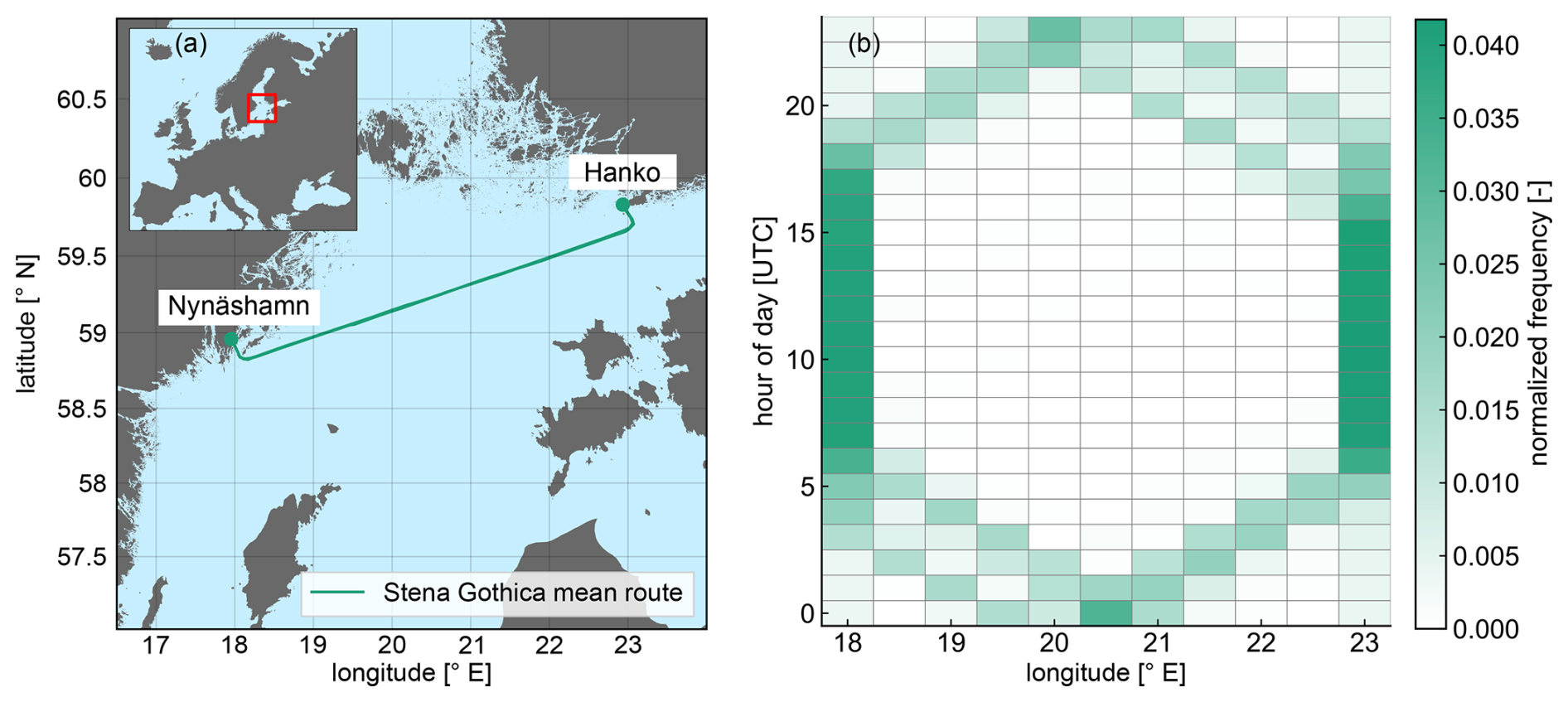
Figure 1 (a) The mean route of the Stena Gothica ferry ship during the execution of the campaign and (b) 2D histogram of the location of the ship depending on the hour of the day and the longitude of its position.

The campaign took place from 28 June 2022 until 21 February 2023. As in Gottschall et al. (2018), the Fraunhofer IWES's in-house-developed ship-based lidar system was used with a vertical profiling Doppler lidar WindCube WLS7 v2, from the manufacturer Vaisala, configured to measure at 12 different height levels ranging from 60 to 270 m above sea level (a.s.l.). In addition to the lidar device, the integrated ship-based lidar system includes a motion recording unit to track the vessel motions and positions (attitude and heading reference sensor and a satellite compass) and a meteorological station to record the main meteorological parameters, including temperature, pressure, relative humidity, and precipitation.

As in previous ship-based lidar campaigns, a ship-motion compensation algorithm was implemented to take the motion effects out of the measurements. For this, the motion information recorded by the system is used in combination with the wind lidar measurements, applying a simplified motion correction algorithm (Wolken-Möhlmann and Gottschall, 2014). This algorithm considers the translational ship velocity and orientation, ignoring vessel tilting due to its negligible influence on the results. Additionally, lidar measurements with carrier-to-noise ratio (CNR) values below −23 dB were excluded from the final database, following the manufacturer's recommendation to strike a balance between data availability and accuracy. Subsequently, lidar measurements and motion information (i.e. ship coordinates) were averaged into 10 min mean values.

Figure 2 provides insights into the measured data during the campaign. In the first panel, the longitude-binned wind speed at 100 m height can be observed, along with the normalised frequency of 10 min average recordings at each longitude bin. The lowest wind speed corresponds to the longitude bin encompassing the Swedish harbour, with an average velocity of around 6.6 m s⁻¹. This specific location, Nynäshamn harbour, can be considered onshore due to its intricate topography, characterised by numerous small islands and hills that slow down the wind flow. In contrast, the remaining locations are characterised as offshore sites, with mean wind speeds above 8.5 m s⁻¹, with the highest mean speed observed at Hanko harbour.

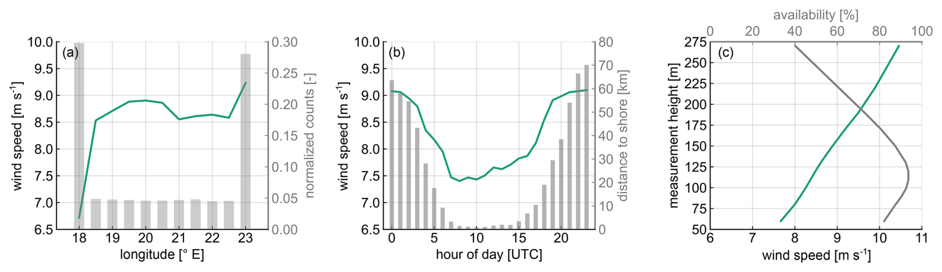
Figure 2 Summary of lidar measurements. (a) Mean wind speed at 100 m height per longitude (green line) and normalised number of 10 min counts per longitude (bars). (b) Wind speed ship daily cycle at 100 m height (green line) and mean distance to shore per hour (bars). (c) Mean wind speed profile (green line) and mean availability during the campaign time extent per measurement height a.s.l. (grey line).

Figure 2b illustrates the wind speed ship daily cycle (represented by the solid line) at 100 m height and the mean distance to the shore per hour (represented by the bars). Minimum wind speeds occur during the central hours of the day, coinciding with the period when the ship is mainly located at the two harbours. Despite Hanko harbour typically presenting stronger wind speeds, the considerably lower wind velocities measured at Nynäshamn and the higher frequency of observations at this site (refer to Fig. 2a) result in a noticeable decrease in the average wind speed during these hours. In contrast, the highest wind speeds are observed during the night and the early morning, when the ship is typically in transit between the two harbours.

Finally, Fig. 2c shows the mean wind speed along the measured wind profile (green line) together with the total availability profile of the lidar during the campaign (grey line). As can be observed, there is a pronounced increase in the mean wind speed with height, going from 7.6 m s⁻¹ at 60 m to 10.4 m s⁻¹ at the top measurement height. The availability profile shows maximum values above 90 % within the range of 80–130 $\mathrm{m}\mathrm{a}.\mathrm{s}.\mathrm{l}.$ range. Beyond 130 m, the availability drops rapidly with height as a consequence of very clean air and low concentration of aerosols in the region and period of study. The decrease in availability at lower levels is explained by the lidar device's focus distance of around 120 $\mathrm{m}\mathrm{a}.\mathrm{s}.\mathrm{l}.$ Moving further below or beyond this distance results in lower CNR values, causing measurements to be filtered out of the dataset when CNR falls below the −23 dB threshold.

2.2 ASCAT

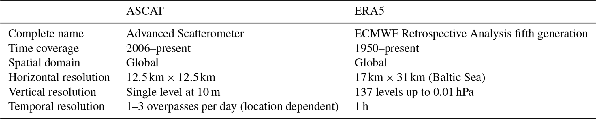
The Advanced Scatterometer (ASCAT) is a space-borne remote sensing instrument that measures radar backscatter from the Earth's surface in the microwave frequency range (Martin, 2014). ASCAT was launched by the European Space Agency (ESA) on board the Meteorological Operation (MetOp) satellites, developed and operated by the European Organization for the Exploitation of Meteorological Satellites (EUMETSAT) (Verhoef and Stoffelen, 2019). MetOp-A was the first satellite launched in October 2006, followed by MetOp-B in September 2012 and by MetOp-C in November 2018. ASCAT provides wind speed and direction measurements at 10 m above the sea surface, with global coverage and available grid spacings of 12.5 and 25 km (de Kloe et al., 2017). For this study, the higher spatial resolution data were selected, as it has shown better performance in previous studies when validated against in situ measurements (Verhoef and Stoffelen, 2013; Carvalho et al., 2017). This dataset is processed and distributed by the EUMETSAT Ocean and Sea Ice (OSI) Satellite Application Facility (SAF) and the Advanced Retransmission Service (EARS). Both systems are managed by the Koninklijk Nederlands Meteorologisch Instituut (KNMI), and the data were downloaded for this study using the Copernicus Marine Data Service (CMS) (product ID: WIND_GLO_WIND_L3_NRT_OBSERVATIONS_012_002).

ASCAT has an effective swath width of 512.5 km with a nadir gap of 700 km, resulting in a temporal resolution of 1–3 overpasses daily considering both the ascending and the descending trajectories, depending on the time period and location (latitude). The number of ASCAT overpasses in the northern Baltic Sea region during the execution of the measurement campaign is presented in Fig. 3a, while the diurnal distribution of the overpasses is shown in Fig. 3b.

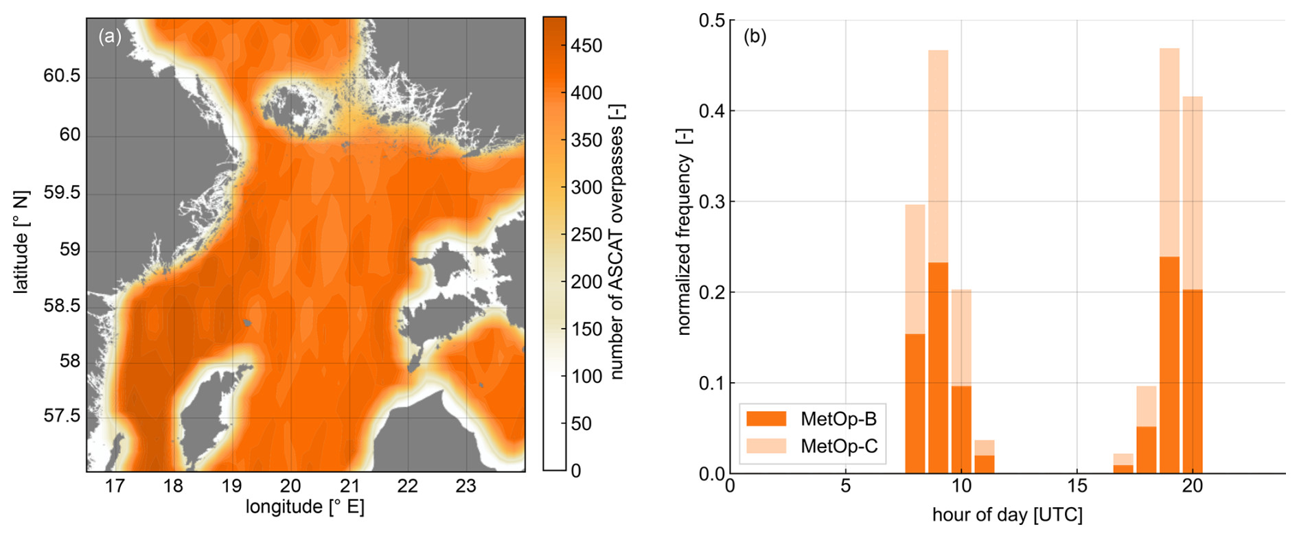
Figure 3 (a) Number of ASCAT overpasses during the duration of the campaign. (b) Normalised frequency of ASCAT overpasses per hour of the day.

The ASCAT scatterometer is an active microwave radar that measures the backscatter power from transmitted pulses operating in the C-band frequency of 5.255 GHz. These measurements are unaffected by cloud cover and rain. The received backscatter is related to the surface roughness of the observed area. It is minimal when the surface is completely smooth, such as during calm weather conditions, and progressively increases as surface roughness intensifies. This backscatter signal is used to calculate the normalised radar cross-section (NRCS, σ₀), defined as the ratio of the received and transmitted power, which depends on the radar settings, the atmospheric attenuation, and the ocean surface characteristics (Chelton et al., 2001). From NRCS and through the application of an empirically derived geophysical model function (GMF), the sea surface winds are calculated. These empirical models are calibrated using in situ measurements of wind speed from buoys and other sources and are validated using independent measurements from other satellite instruments and numerical models (Hersbach et al., 2007; Hersbach, 2008; Verspeek et al., 2012). The current GMF used by ASCAT is the CMOD7 (Stoffelen et al., 2017), which was developed by the ESA specifically for use with C-band scatterometers.

The implemented ASCAT data processing for this study focused on satellite measurements retrieved during the period of the ship-based lidar measurement campaign and included the following main steps. Firstly, a coordinate transformation was applied to transfer ASCAT coordinate points from the bottom left corner of each grid box to the centre of the box. Subsequently, a quality check was conducted by filtering out measurements based on the quality flags provided by the CMS (E.U. Copernicus Marine Service Information (CMEMS), 2023), which account for factors such as the presence of sea ice, extreme wind conditions (wind speeds below 3 m s⁻¹ or above 30 m s⁻¹), and proximity to land. Despite the application of these quality filters, ASCAT seems to overestimate wind speeds near the coast (see Sect. 3), likely due to coastal contamination effects (Stoffelen et al., 2008; Lindsley et al., 2016). To address this, an interquartile range (IQR) outlier detection method (Dekking, 2005) was employed, identifying grid boxes with unusually high wind speed values and masking them out from the analysis.

2.3 ERA5

ERA5 (ECMWF Reanalysis fifth generation) is the latest global atmospheric reanalysis produced by the European Centre for Medium-Range Weather Forecasts (ECMWF) (Hersbach et al., 2020). ERA5 replaces the previous reanalysis ERA-Interim (Dee et al., 2011) and is based on the latest version of the Integrated Forecasting System (IFS) model IFS Cycle 41r2. ERA5 provides hourly estimates of a wide range of atmospheric, land surface, and oceanic variables with a 0.25°×0.25° latitude–longitude grid resolution, covering the period from 1950 to present. Additionally, ERA5 uses 137 model (pressure) levels extending from the surface level to the top of the atmosphere at 0.01 hPa or around 80 km height. ERA5 is produced using an assimilation scheme based on the four-dimensional variational (4D-Var) system (Bonavita et al., 2016). This method integrates modelled data from the IFS with observational data from a range of sources such as satellites (ASCAT among them), radiosondes, and aircraft widespread across the world.

Table 1 Mean characteristics of ASCAT and ERA5.

For this study, the u and v wind components were downloaded for the lowest 10 model levels to calculate the horizontal wind speed and direction. Additionally, the surface sensible heat flux, air temperature at 2 m above the surface, and the friction velocity parameters were also downloaded to derive the atmospheric stability information required for ASCAT winds extrapolation (see Sect. 2.4). Furthermore, the ERA5 data were re-gridded to match the ASCAT wind speed maps resolution (0.125° latitude and longitude) using bilinear interpolation. It should be noted that only ERA5 data within the time frame of the measurement campaign have been used in this study.

2.4 Satellite vertical extrapolation

One of the main limitations of the application of satellite remote sensing measurements in the field of wind energy is that they provide wind information only at surface level. Consequently, vertical extrapolation methods must be implemented to obtain wind information at wind turbine hub heights. Several methodologies for vertical extrapolation of satellite measurements have been explored in the previous literature. For example, Capps and Zender (2009, 2010) used 10 m wind measurements from QuickSCAT to estimate the global wind power potential at various vertical levels. In their approach, the Monin–Obukhov similarity theory (MOST) was implemented for the atmospheric stability correction of the vertical wind profile, using data from a global ocean–surface heat flux product and reanalysis data. Doubrawa et al. (2015) employed the equivalent neutral winds from QuickSCAT and synthetic aperture radar (SAR) along with a neutral logarithmic profile to calculate a wind atlas in the Great Lakes region. Similarly, Badger et al. (2016) and Hasager et al. (2020) extrapolated SAR and ASCAT surface winds using the mean stability correction presented in Kelly and Gryning (2010), a method based on a probabilistic adaptation of the MOST-based wind profile. Finally, Hatfield et al. (2023) developed a machine-learning model to extrapolate ASCAT winds to wind turbine operating heights, employing 12 years of satellite wind observations in conjunction with near-surface atmospheric measurements at FINO3 and comparing the output wind profiles against both in situ measurements and numerical model data.

In this study, we employ the approach used by Badger et al. (2016) and Hasager et al. (2020) to calculate the ASCAT wind profiles. This method involves a mean correction of atmospheric stability effects, obtained from the numerical model dataset ERA5, alongside a probabilistic adaptation of the MOST-based wind profile to vertically extrapolate the satellite wind measurements. The mean stability correction factor derived from this methodology can exhibit both positive and negative stability corrections depending on the height considered, as it combines stable and unstable terms. Conversely, when applying stability correction factors to instantaneous wind speed measurements, the stable or unstable terms are applied separately.

There are two primary methods for stability correction: mean stability correction and instantaneous stability correction. Compared to the instantaneous stability correction approach, applying the mean stability correction avoids the need to calculate wind speeds under stability conditions and heights that fall out of the validity range of the MOST model. MOST is specifically designed to describe turbulent fluxes within the surface layer (Lange et al., 2004; Högström et al., 2006) but has limitations when dealing with instantaneous data analysis, particularly in stable conditions. The statistical adaptation of MOST can be applied effectively up to turbine operating heights, since the mean stability correction remains within the range where MOST is applicable. In neutral and unstable conditions, MOST can be successfully employed within the lower 200 km of the vertical profile (Peña et al., 2008).

Another advantage of the mean stability correction is that the numerical models used for this method can reliably capture the average meteorological conditions over extended periods (Peña and Hahmann, 2012). In contrast, the accuracy of these models in capturing instantaneous stability information is questionable, introducing additional uncertainty into extrapolated profiles based on instantaneous data (Badger et al., 2012). Furthermore, while the previous literature highlighted the good performance of data-based extrapolation methods (Optis et al., 2021; de Montera et al., 2022; Hatfield et al., 2023), the limited time span of the measurement campaign and the low temporal resolution of ASCAT result in an insufficient amount of data to implement these approaches in this study. However, a major drawback of the mean stability correction is that it averages out time-specific information, ignoring the impact of certain mesoscale phenomena on the mean wind profile.

The implementation of the mean stability correction approach is described below. This is individually executed for each of the ASCAT grid points using the stability information from the ERA5 corresponding location. As a result of this process, one ASCAT-derived mean profile is calculated for each grid point.

The atmospheric stability can be directly accounted for by the estimated Obukhov length L parameter, calculated as

$$\begin{array}{}\text{(1)}& {\displaystyle }{\displaystyle }L=-{\displaystyle \frac{\stackrel{\mathrm{‾}}{T}{u}_{*}^{\mathrm{3}}}{\mathit{\kappa }g\stackrel{\mathrm{‾}}{w^{\prime }{\mathit{\theta }}_{\mathrm{v}}^{\prime }}}},\end{array}$$

where $\stackrel{\mathrm{‾}}{T}$ is the air temperature, u_* is the friction velocity, κ is the von Kármán constant (≈0.4), g is the Earth's gravitational acceleration, $\stackrel{\mathrm{‾}}{w^{\prime }{\mathit{\theta }}_{\mathrm{v}}^{\prime }}$ is the kinetic virtual heat flux, where w^′ is the vertical component of the wind speed, and ${\mathit{\theta }}_{\mathrm{v}}^{\prime }$ is the virtual potential temperature. The temporal means are denoted by overbars, while fluctuations around the mean value are indicated by primes. Accurate measurements of heat and momentum fluxes require three-dimensional observations from high-frequency sonic anemometers. However, since we wish to develop an extrapolation method independent from in situ measurements, the mean temperature and heat fluxes in Eq. (1) are replaced by the ERA5 parameters air temperature at 2 m and surface sensible heat flux, respectively. Additionally, friction velocity values from ERA5 are also utilised. Positive values of the inverse Obukhov length $\mathrm{1}/L$ denote stable atmospheric conditions, negative values indicate unstable conditions, and values around 0 indicate near-neutral stratification.

According to the formulation described in Kelly and Gryning (2010), the probability density function P of $\mathrm{1}/L$ can be estimated as

$$\begin{array}{}\text{(2)}& {\displaystyle }{\displaystyle }P\left(L^{-\mathrm{1}}\right)=n_{\pm }{\displaystyle \frac{C_{\pm }}{{\mathit{\sigma }}_{\pm }}}{\displaystyle \frac{\exp \left[-{\left(C_{\pm }|\mathrm{1}/L|/{\mathit{\sigma }}_{\pm }\right)}^{\mathrm{2}/\mathrm{3}}\right]}{\mathrm{\Gamma }[\mathrm{1}+\mathrm{3}/\mathrm{2}]}},\end{array}$$

where the subscripts + and − indicate the stable and unstable portions of the distribution, respectively; n_± indicates the fractions of occurrence of each portion, C_± indicates semi-empirical constants, and σ_± indicates the scale of variations in $\mathrm{1}/L$, based on the mean standard deviation of the surface heat flux and the average of the cube of the friction velocity, as indicated in the equation below:

$$\begin{array}{}\text{(3)}& {\displaystyle }{\displaystyle }{\mathit{\sigma }}_{\pm }={\displaystyle \frac{g}{\langle \stackrel{\mathrm{‾}}{T}\rangle }}{\displaystyle \frac{\sqrt{\langle (\stackrel{\mathrm{‾}}{w^{\prime }{\mathit{\theta }}_{\mathrm{v}}^{\prime }}-\langle \stackrel{\mathrm{‾}}{w^{\prime }{\mathit{\theta }}_{\mathrm{v}}^{\prime }}{\rangle }_{\pm }{)}^{\mathrm{2}}\rangle }}{\langle u_{*}^{\mathrm{3}}\rangle }}.\end{array}$$

As for Eq. (1), we replace the mean temperature and heat fluxes with the corresponding parameters provided by ERA5.

In this study, the values for the constants C_± have been set to 6 and 4 for the stable and unstable portions, respectively. Although previous studies focused on different datasets have used other values (e.g. both set to 3 in Badger et al., 2016; and $C_{+}=\mathrm{5}$ and $C_{-}=\mathrm{12}$ in Optis et al., 2021), the selection of these values for this study was based on empirical validation, comparing the theoretical distribution calculated from Eq. (2) against the normalised probability density (NPD) function of $\mathrm{1}/L$ derived from ERA5. Through this process, values were chosen to ensure that the theoretical distribution closely represented the ERA5 NPD of $\mathrm{1}/L$ across all ASCAT grid boxes along the entire ship route. Furthermore, identical values of C_± were applied to all ASCAT grid points.

Finally, the mean stability correction of the mean wind profile at a specific height z is calculated as

$$\begin{array}{}\text{(4)}& {\displaystyle }{\displaystyle }{\mathrm{\Psi }}_{\mathrm{m}}^{*}=-n_{+}{\displaystyle \frac{\mathrm{3}{\mathit{\sigma }}_{+}}{C_{+}}}{b}^{\prime }z+n_{-}{f}_{-},\end{array}$$

where b^′ is calculated as

$$\begin{array}{}\text{(5)}& {\displaystyle }{\displaystyle }{b}^{\prime }={\displaystyle \frac{b}{\mathrm{\Gamma }[\mathrm{1}+\mathrm{3}/\mathrm{2}]}},\end{array}$$

with b=4.7 coming from the standard MOST formulation for stable conditions ${\mathrm{\Psi }}_{\mathrm{m}}=bz/L$ (Stull, 1988). Analogously, f₋ is derived from the standard MOST formulation for unstable conditions (see Kelly and Gryning, 2010, for the exact formulation of f₋).

To evaluate the potential influence of the discretised temporal frequency of ASCAT overpasses, and therefore the effect of the available stability information on the derivation of the mean stability correction factor, two different approaches have been compared. First, in the so-called collocated approach, only ERA5 stability information at times collocated with the ASCAT overpasses was considered. In the second approach, all ERA5 stability information from the entire duration of the campaign was used. The normalised probability density functions of atmospheric stability ($\mathrm{1}/L$) derived from ERA5 at two different locations along the ship's route are shown in Fig. 4, together with the theoretical distribution calculated from Eq. (2) for the two approaches considered.

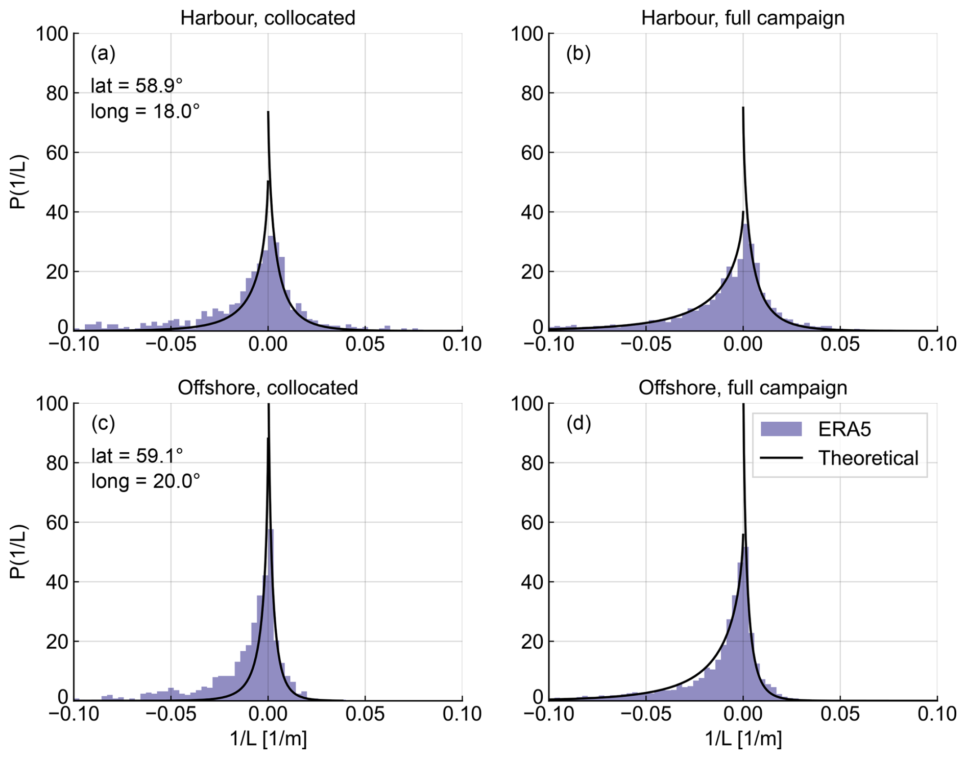
Figure 4 Normalised probability density functions of inverse Obukhov length $\mathrm{1}/L$ from ERA5 and theoretical distributions calculated from Eq. (2). Panels (a) and (c) depict the collocated approach, employing ERA5 stability information only from timestamps coinciding with ASCAT overpasses, while panels (b) and (d) illustrate the full campaign approach, incorporating ERA5 stability information for the entire duration of the measurement campaign. Results are presented for two grid points: one offshore site (c, d) and one location near Nynäshamn harbour (a, b). The coordinates of these sites are indicated in panels (a) and (c), respectively.

The left panels show the collocated approach, employing ERA5 stability information from timestamps coinciding with ASCAT overpasses, while the right panels depict the full campaign approach, incorporating ERA5 stability information for the entire duration of the measurement campaign. Results are presented for two grid points: one offshore site (panels c and d) and one location near Nynäshamn harbour (panels a and b). The coordinates of these sites are indicated in panels a and c, respectively.

As observed, considering the stability information from the full campaign results in a better theoretical distribution compared to the collocated approach. Although the difference is minimal at the harbour site, it is more pronounced at the offshore location, where a significant underestimation of the unstable stability frequency is observed. The harbour site presents a rather symmetric distribution around zero, meaning that both unstable and stable atmospheric conditions are equally represented. However, the offshore site exhibits a higher occurrence of unstable conditions compared to the stable side of the curve. Section 3.1 presents additional results on this matter and evaluates the differences in the ASCAT wind profiles obtained between the two approaches.

Finally, the extrapolated wind speed at any desired height z can be calculated from Eq. (6) by introducing the mean stability correction ${\mathrm{\Psi }}_{\mathrm{m}}^{*}$ obtained from Eq. (4):

$$\begin{array}{}\text{(6)}& {\displaystyle }{\displaystyle }U\left(z\right)={\displaystyle \frac{\langle u_{*}\rangle }{\mathit{\kappa }}}[\ln \left({\displaystyle \frac{z}{\langle z_{\mathrm{0}}\rangle }}\right)-{\mathrm{\Psi }}_{\mathrm{m}}^{*}].\end{array}$$

2.5 Collocation procedure

The comparison of gridded datasets (ERA5 and ASCAT) against the non-stationary measurements from the ship-based lidar system requires the implementation of a collocation methodology to ensure a fair comparison. Previous studies have already conducted comparisons between gridded data and ship-based lidar measurements (Witha et al., 2019b; Hatfield et al., 2022; Rubio et al., 2022). However, unlike the previous literature that focuses on time–space collocated comparisons, in this study, ship-based lidar measurements are compared against the mean wind profiles calculated for each of the grid points from the gridded datasets. Consequently, a novel methodology for collocating and comparing the mean gridded and lidar-measured wind profiles has been developed and is briefly introduced in this section.

After applying the coordinate transformation and re-gridding procedures explained in Sect. 2.2 and 2.3, both datasets are gridded with an identical discretisation, featuring a horizontal resolution of 0.125°×0.125° and the grid points located at the centre of the grid boxes, as shown in Fig. 5. For each grid box, the ERA5 mean profile is calculated for the period of the measurement campaign, while the mean ASCAT profile is obtained using the procedure described in Sect. 2.4. To obtain the mean lidar profiles for comparison, the 10 min average ship position information is utilised to identify all the 10 min lidar measurements captured within each grid box. Subsequently, the mean lidar profile for each grid point is calculated by averaging all the 10 min measurements detected in the corresponding grid box. This enables the comparison of all ERA5 and ASCAT grid boxes with their respective mean wind profiles against the collocated “gridded” lidar mean profile. The collocation procedure is summarised in Fig. 5, where example ship coordinates are depicted as coloured dots, corresponding to the colour of the grid box used to derive the mean profile.

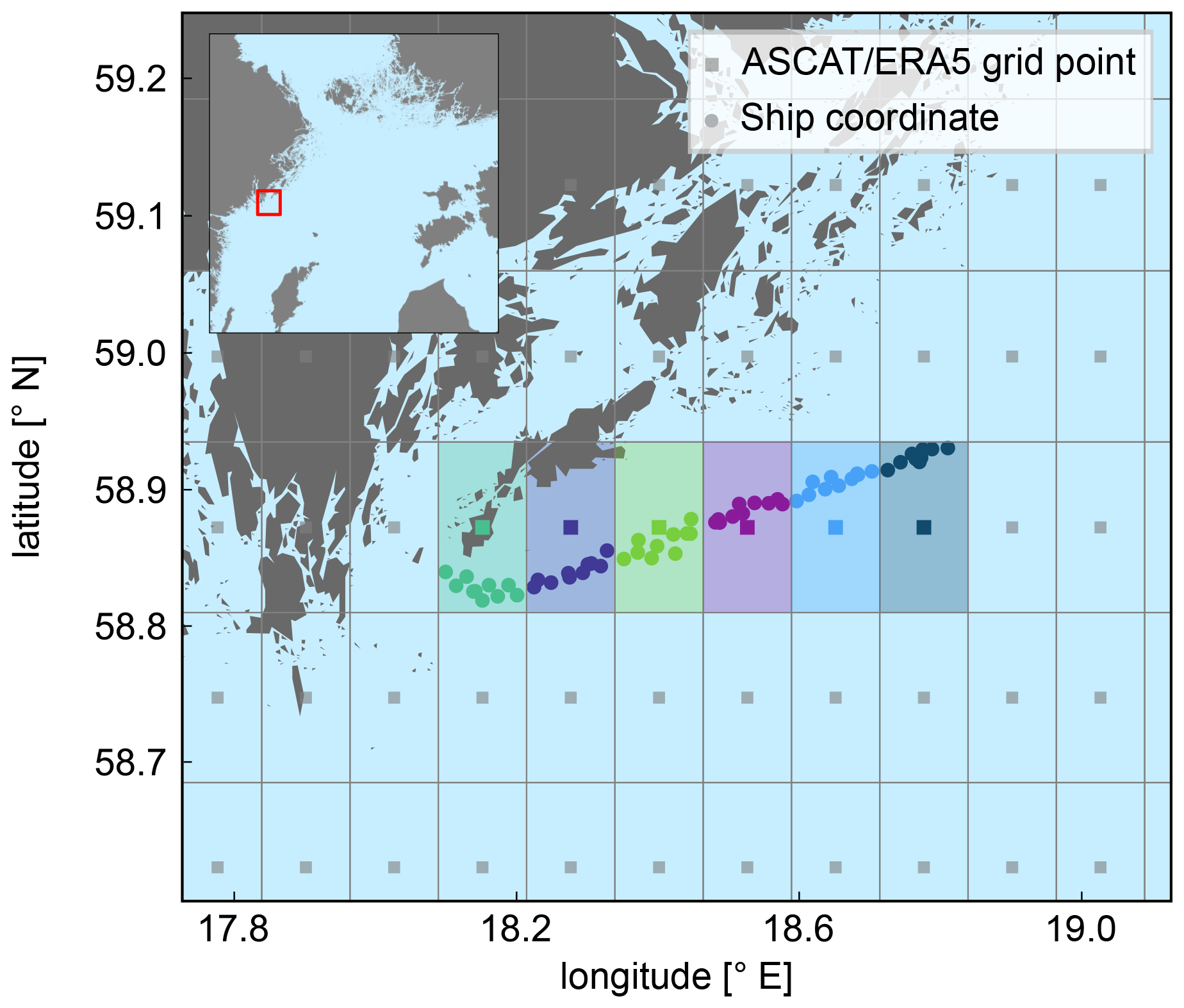
Figure 5 Collocation procedure sketch illustrating the comparison of lidar-measured wind profiles against ERA5 and ASCAT profiles. The grey grid represents the ASCAT and ERA5 grid boxes after the coordinate transformation of ASCAT and the ERA5 re-gridding procedure. For each coloured grid box, all lidar measurements performed within that area (depicted as dots of the corresponding colour) are averaged to calculate the corresponding lidar profile.

It should be noted that grid boxes with less than 24 h of lidar data available (equivalent to 144 10 min samples) are excluded from the comparison. Figure 6 illustrates the count of 10 min lidar samples considered within each ASCAT grid box along the ship route. As observed, grid boxes corresponding to harbour locations exhibit the highest count of lidar retrievals, as the ship remains stationary for longer periods in these areas. In contrast, the grid boxes along the rest of the vessel route exhibit varying counts of data, ranging from 144 samples to around 400 in most of the grid boxes. Furthermore, Figs. 5 and 6 show that the surface of certain ASCAT grid boxes, particularly those at or near the two harbours, is partially covered by land. The influence of this effect is discussed in the results section of this study, where its potential impact on the presented findings becomes apparent.

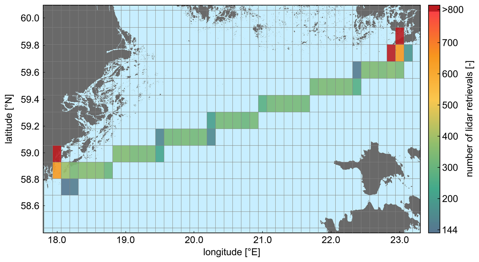
Figure 6 Number of 10 min lidar samples recorded at each ASCAT grid cell. Only grid cells with more than 24 h of lidar data (or 144 10 min samples) are coloured, while cells with fewer data are excluded.

3 Results

The main results of this study are presented in this section. First, Sect. 3.1 compares the extrapolated ASCAT values obtained through the two collocation approaches employed to derive the mean stability correction factor. This analysis highlights the effect of ASCAT overpasses' discrete temporal resolution and ERA5 coarse horizontal resolution in the derived mean stability distribution and, consequently, on the extrapolated wind speed at 100 m. Then, a comparative analysis between ERA5 and ASCAT at 10 and 100 m heights is conducted within the northern Baltic Sea region. Through this comparison, we evaluate the different characterisation of wind speeds represented by the two datasets over the whole area, with a particular emphasis on factors such as coastal contamination and the effect of the employed extrapolation methodology on the discrepancy between the datasets. Finally, Sect. 3.3 focuses on validating the extrapolated ASCAT and ERA5 wind speed profiles by comparing them against the reference measurements from the ship-based lidar.

In order to validate the wind profiles derived from ASCAT and ERA5 against the lidar in different locations, these comparisons are performed at six locations indicated in Fig. 7. The selection of these locations aims to represent the different wind conditions along the route, including locations near the shore as well as far offshore sites.

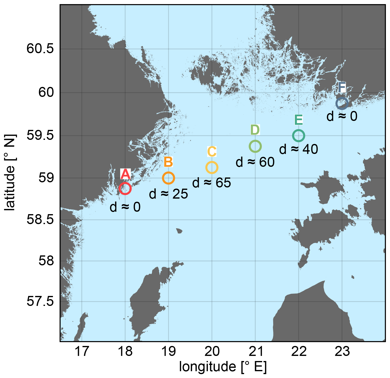
Figure 7 Six locations used for the comparison of the datasets. The approximate distance to the nearest shore is indicated (in km) below of each site. Location A corresponds the harbour of Nynäshamn (Sweden), and location D corresponds to Hanko harbour (Finland).

3.1 Influence of stability information in ASCAT profiles

As explained in Sect. 2.4, two different collocation approaches have been considered for the characterisation of the stability from ERA5 parameters and the corresponding derivation of the mean stability correction. This section investigates the effects of both approaches in the obtained ASCAT wind profiles.

Figure 8 illustrates the differences in wind speed at 100 m height between the collocated and the full campaign approach. Overall, the wind speed discrepancy remains minimal in most of the study area. In the open sea, the agreement is particularly strong, with differences typically below 0.15 m s⁻¹. However, more significant discrepancies are reported in areas near the shore, where wind speed biases reach up to approximately 0.4 m s⁻¹. Notably, the region surrounding the Swedish harbour of Nynäshamn exhibits the largest differences.

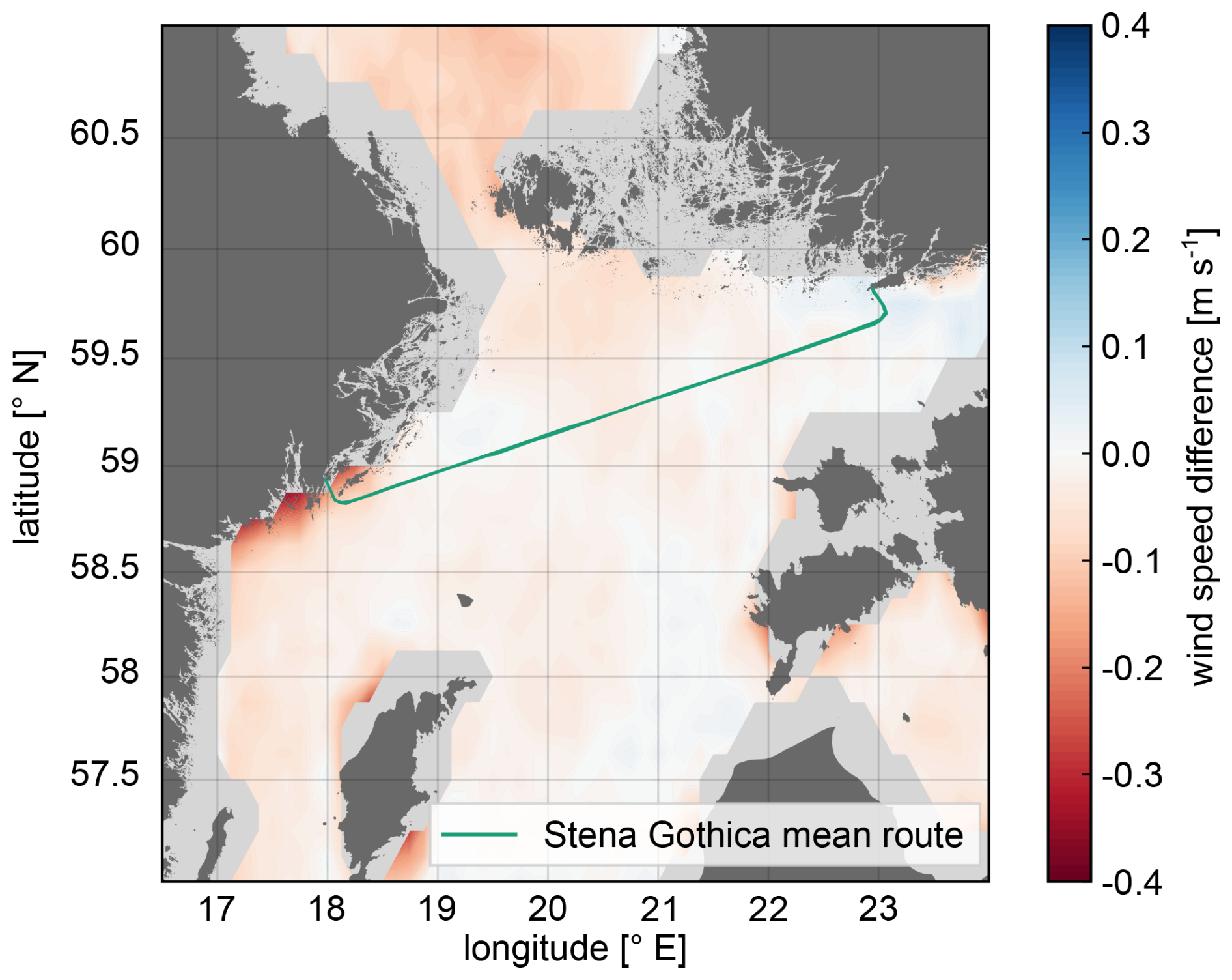
Figure 8 Mean wind speed difference at 100 m height, calculated as the collocated approach minus the full campaign approach.

The lower values associated with the collocated approach can be explained by two primary factors. Firstly, as mentioned in Sect. 2.4, the same values of the semi-empirical constant C_± are assumed for the entire region, instead of using a site-specific definition of these constants. Therefore, the suitability of the selected values may not be optimal for certain locations, leading to an anomalous theoretical representation of the empirical atmospheric distribution.

Secondly, the temporal discretisation of ASCAT overpasses, occurring at roughly the same time each day, influences the resulting mean stability distribution “seen” by the collocated approach. This is illustrated in Fig. 9, which depicts the daily cycle of the mean stability ($\mathrm{1}/L$) at the six locations A–F presented in Fig. 7. As can be observed, the more unstable conditions just before midday at Nynäshamn harbour due to ERA5 land contamination (red line) have a larger influence on the mean stability assessment when considering only the collocated periods (orange-shaded areas in Fig. 9) rather than the full period. In locations like this, with predominantly unstable conditions, the mean stability correction factor has a positive sign and increases as the frequency of unstability (n₋) rises. Consequently, the larger influence of unstable conditions in the collocated approach results in lower wind speeds compared to the full campaign approach, as derived using the equations described in Sect. 2.4. This unstability at location A is attributed to the coarse resolution of ERA5, resulting in land contamination of the grid box at the harbour location, where land covers 56 % of the grid box surface. Therefore, the daily stability cycle is more similar to that of an onshore site. From 05:00 to 08:00 UTC, the transition from night-time to daytime triggers a decrease in the $\mathrm{1}/L$ value as the surface warms with the sunrise, fostering increased turbulence and vertical mixing in the atmosphere. The period of highest unstability then occurs around midday when the surface heating is more intense. Throughout the afternoon and evening, as surface heating decreases, so does turbulence, developing a more stable boundary layer. Unstability reaches its minimum (the negative value of $\mathrm{1}/L$ closest to 0) in the late evening and remains relatively constant until the following morning.

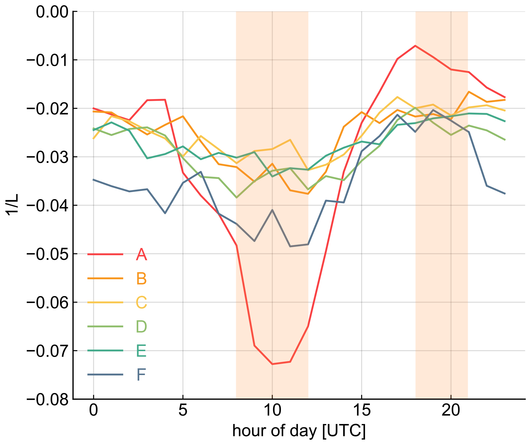
Figure 9 Daily cycle of the stability parameter ($\mathrm{1}/L$) at the six evaluated locations A–F from Fig. 7. All values of $\mathrm{1}/L$ are below zero indicating an unstable atmosphere. Location A corresponds to the harbour of Nynäshamn (Sweden) and location F to the harbour of Hanko (Finland). The orange-shaded areas indicate the time periods when ASCAT overpasses are available and are therefore the only periods included in the collocation approach.

In contrast, locations B–E are purely offshore (with a land fraction of 0 %) and therefore exhibit almost no diurnal cycle because the stability is mainly determined by the seawater temperature. This leads to smaller temperature variations and a more stable boundary layer. Finally, at Hanko harbour (location F), the daily stability cycle is more pronounced than offshore but weaker than at Nynäshamn harbour (location A). Two main factors account for the difference between the two harbours: (1) the grid box at Hanko contains a significantly lower land fraction (6 % compared to 56 % at Nynäshamn), and (2) with predominantly W–SW winds, the wind at Hanko (F) is predominantly sea-to-land, whereas at Nynäshamn, it is land-to-sea.

Both strategies for calculating the stability correction factor and the corresponding wind profiles demonstrate a high level of agreement, except for some nearshore locations. This, together with the revealed representativeness of the theoretically derived stability distributions observed in Fig. 4, highlights the robustness of the mean stability correction approach in characterising the atmospheric stability conditions, independently of the approach used, during the period covered by the measurement campaign and, particularly, across open sea regions. Given the minimal differences in the wind speeds at 100 m depicted in Fig. 8, and thus the similar wind profiles obtained using both approaches, subsequent sections of this paper will only consider the full campaign approach for the sake of clarity and conciseness, since comparing both would not yield sufficiently significant differences. This approach is expected to provide more representative wind profiles along the complete ship route, as more stability information is included for the derivation of the mean ASCAT profiles.

3.2 ASCAT-derived vs. ERA5 wind speeds

The offshore mean wind speeds based on ASCAT and ERA5 in the northern Baltic Sea region at 10 and 100 m heights are compared in Fig. 10. For an easier comparison, only grid points with ASCAT data available are included, and the same colour scale is used for the four plots.

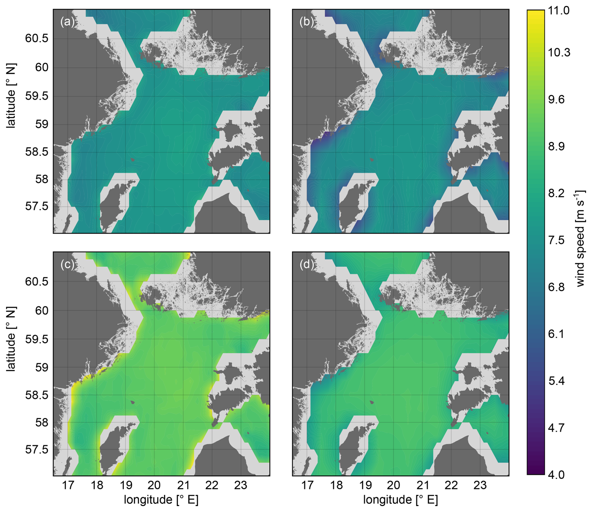
Figure 10 Mean wind speed for the campaign period at 10 m (a, b) and 100 m (c, d) for ASCAT (a, c) and ERA5 (b, d).

As can be observed when comparing the spatial variation shown by the two datasets at 10 m, ERA5 exhibits higher mean wind speeds in offshore areas farthest from the coast and lower wind speeds closer to shore. This is due to ERA5's relatively coarse grid box size, which leads to land contamination in the grid cells near the coast. As a result, surface roughness is overestimated, and consequently 10 m wind speeds are underestimated. The impact of prevailing W–SW winds is also evident, with more pronounced land effects in regions where winds typically blow from land toward sea, such as along the Swedish coastline. Similar effects can be seen at 100 m height. For ASCAT, higher wind speeds are also observed in the central part of the basin. However, unlike ERA5, some areas close to shore exhibit slightly higher wind speed values. In these regions, ASCAT measurements may be influenced by factors such as wave breaking and surface slicks, which can result in anomalously high wind field measurements (Johannessen, 2005; Kudryavtsev, 2005), potentially caused by the numerous small inlets in some coastal regions (e.g. near Nynäshamn harbour). This effect is particularly visible on the ASCAT 100 m height map, where the highest mean wind speeds are located along the perimeter of the region with available data.

As to be expected, both datasets consistently show higher wind speeds at 100 m than at 10 m height. For 10 m height, the wind speed averaged over all included grid points is 7.61 m s⁻¹ (ASCAT) and 7.15 m s⁻¹ (ERA5), which means that the difference (${\stackrel{\mathrm{‾}}{U}}_{\text{ASCAT}}-{\stackrel{\mathrm{‾}}{U}}_{\text{ERA5}}$) is 0.46 m s⁻¹. When only locations more than 20 km from the coast are considered, this difference reduces to approximately 0.16 m s⁻¹. In contrast, only including locations within 20 km from the shore increases this difference to 0.98 m s⁻¹. Similar findings were reported in Duncan et al. (2019a) in their comparison of ASCAT and ERA5 wind speeds at 10 m over the North Sea and the Dutch coast, where a nearly zero deviation in far-offshore locations and approximately 0.6 m s⁻¹ in coastal regions were reported.

For 100 m height, the wind speed averaged over all included grid points is 9.31 m s⁻¹ (ASCAT) and 8.67 m s⁻¹ (ERA5) and the difference 0.64 m s⁻¹. If only more than 20 km from shore locations are included, the difference is reduced to 0.43 m s⁻¹. The difference in bias observed between 100–10 m in ASCAT and ERA5 can be attributed to two key factors: first, the inherent differences between the datasets at 10 m and, second, the mean stability correction approach applied to extrapolate ASCAT.

Figure 11a illustrates the difference in wind speed between ASCAT and ERA5 at 10 and 100 m, plotted as a function of the distance from the shore (calculated from the centre of each grid box). Additionally, the probability distribution of the wind speed differences for the two datasets at the aforementioned heights is presented in Fig. 11b. As can be observed, there is a clear correlation between the distance from shore and the agreement between ASCAT and ERA5 at both heights. Generally, ASCAT presents higher wind speeds than ERA5 in most grid points, with larger differences closer to the coast, which are more pronounced at the 100 m than at the 10 m level. These larger differences in nearshore areas can be explained by the combination of excessively high wind speeds retrieved by ASCAT due to coastal contamination and ERA5's inability to properly resolve the coastal atmospheric phenomena and small-scale wind flow variations due to its coarse horizontal resolution. The differences become smaller moving further offshore and almost negligible at distances further than 40 km from the shore: around 0.2 m s⁻¹ at 10 m height and 0.4 m s⁻¹ at 100 m height.

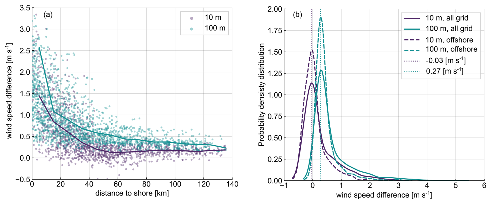
Figure 11 (a) Wind speed difference at 10 and 100 m for ASCAT minus ERA5 at 10 and 100 m as a function of the distance to the shore. (b) Probability density distribution of the wind speed difference at 10 and 100 m for ASCAT minus ERA5. Solid lines for the whole grid and dashed lines for grid points more than 20 km away from the shore. The dotted lines mark the maximum for each of the distribution.

As observed in Fig. 11b, the 10 m height error density distribution is approximately centred around zero bias, while the distribution at 100 m is slightly positively biased, highlighting the consistent larger values of extrapolated ASCAT wind speeds at this height compared to ERA5. Nonetheless, the majority of grid points exhibit wind speed differences below ±1 m s⁻¹. The probability density function of grid points located more than 20 km away from the shore presents a more pronounced peak near the maximum of the corresponding distribution and appears to be more squeezed, indicating that wind speed differences exceeding approximately 1.5 m s⁻¹ primarily correspond to nearshore grid points affected by coastal contamination effects. A similar error distribution was observed in Hasager et al. (2020), when comparing ASCAT and the Weather Research and Forecasting (WRF) model over the European seas.

3.3 Comparison against ship-based lidar measurements

The overall mean profiles obtained for each of the employed datasets and averaged along the entire ship route are presented in Fig. 12a. Additionally, the mean wind profiles are shown for each of the six locations A–F defined in Fig. 7. The non-stability corrected logarithmic profiles are included for comparison (i.e. term ${\mathrm{\Psi }}_{\mathrm{m}}^{*}$ from Eq. 4 set to zero).

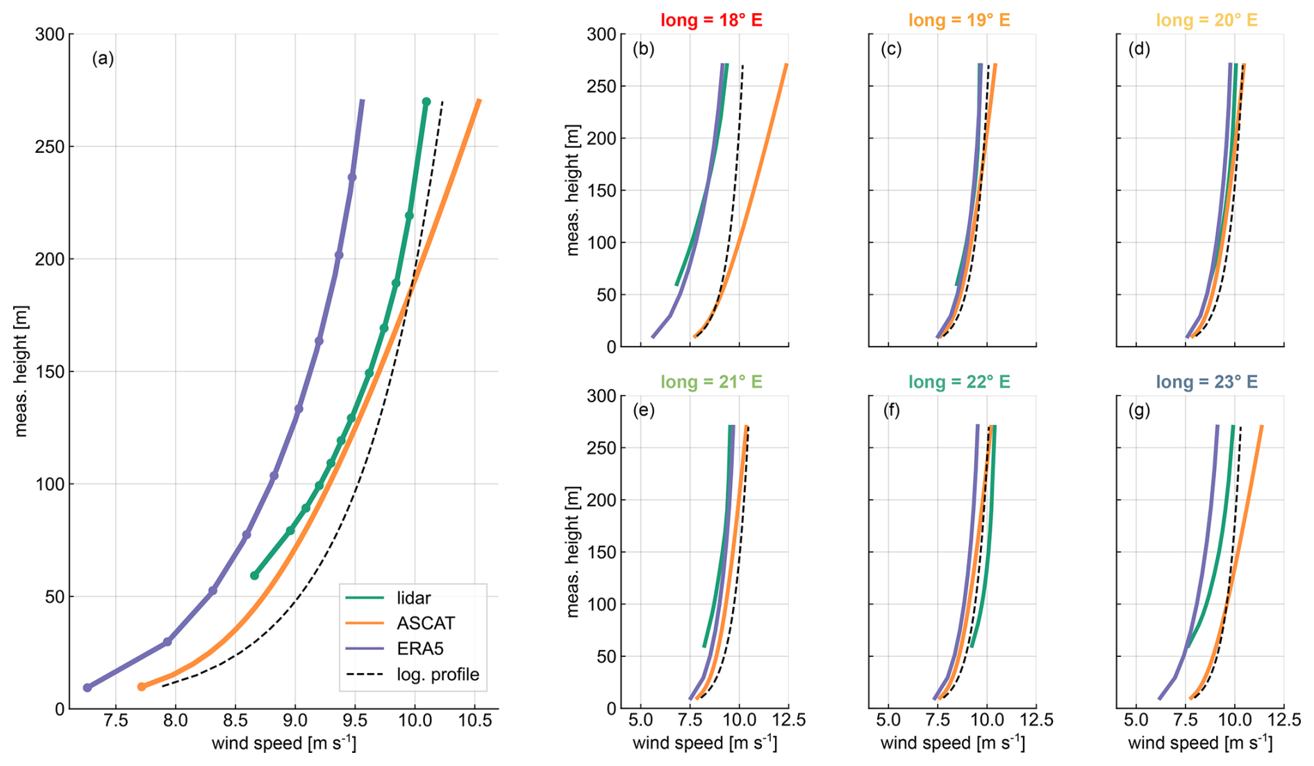
Figure 12 (a) Mean profiles for the three datasets averaged along the whole ship route. The vertical levels with available data/measurements are indicated by circular markers for each dataset. (b–g) Mean profiles for the three datasets at the six evaluated positions. In every panel, the logarithmic profile (non-stability corrected) is indicated by the black dashed line.

As observed, the accuracy of the overall mean profiles depends on the height and dataset considered. Compared to lidar data, ERA5 consistently underestimates the wind speed by approximately 0.5 m s⁻¹ throughout the entire profile, which aligns with the findings of previous studies (Kalverla, 2019; Knoop et al., 2020; Rubio et al., 2022). Conversely, ASCAT's overall mean profile bias is consistently positive (indicating ASCAT overestimation compared to the lidar measurements), with the magnitude depending on the considered height. Both ERA5 and lidar profiles exhibit a similar shear within the height range covered by the lidar measurement, ranging from 8.4 to 9.6 m s⁻¹ for ERA5 and from 8.7 to 10.0 m s⁻¹ in the case of the lidar. In contrast, the ASCAT profile struggles to characterise shear outside the surface layer, with wind speeds ranging from 8.9 m s⁻¹ at 60 m height to 10.5 m s⁻¹ at 270 m. The ASCAT bias becomes increasingly pronounced above 200 m height; beyond this threshold, the logarithmic profile outperforms the stability-corrected profile. This is because these heights exceed the applicability range of the extrapolation methodology used (Kelly and Gryning, 2010).

Although the ASCAT wind profiles, on average, appear to outperform ERA5 in terms of overall accuracy, Fig. 12b–g reveal that the performance of both datasets strongly depends on the location considered. In the case of the harbour locations, ERA5 significantly outperforms ASCAT profiles, which overestimates the wind speed even at 10 m height, highlighting the influence of coastal contamination at these sites. Furthermore, a significant difference is observed between the ASCAT stability-corrected and logarithmic profiles at harbour locations, particularly above 50–100 m, mainly driven by the introduction of the stability correction factor that leads to higher wind speed estimates compared to the logarithmic profile. For the remaining locations, both datasets demonstrate a comparable agreement with the lidar wind profiles.

A statistical analysis of the wind speed deviation between ASCAT and ERA5 compared to lidar observations ($\mathrm{\Delta }{U}_{\text{ASCAT}}=U_{\text{ASCAT}}-U_{\text{lidar}}$ and $\mathrm{\Delta }{U}_{\text{ERA5}}=U_{\text{ERA5}}-U_{\text{lidar}}$) is presented in Fig. 13 in the form of a box plot. Each box plot is calculated considering the wind speed difference of all grid boxes with lidar data along the entire route of the ship, but grid boxes closer than 20 km away from the shore have been excluded to minimise the effect of ASCAT coastal contamination in the derived statistics. The black line corresponds to the mean, the coloured box marks the 25th and 75th percentiles, and the whiskers indicate the data extremes calculated as 1.5 times the interquartile range. Outliers outside the whiskers are hidden to maintain clarity and readability. The continuous lines represent the root mean square error (RMSE) of the wind speed difference between the gridded dataset and the lidar.

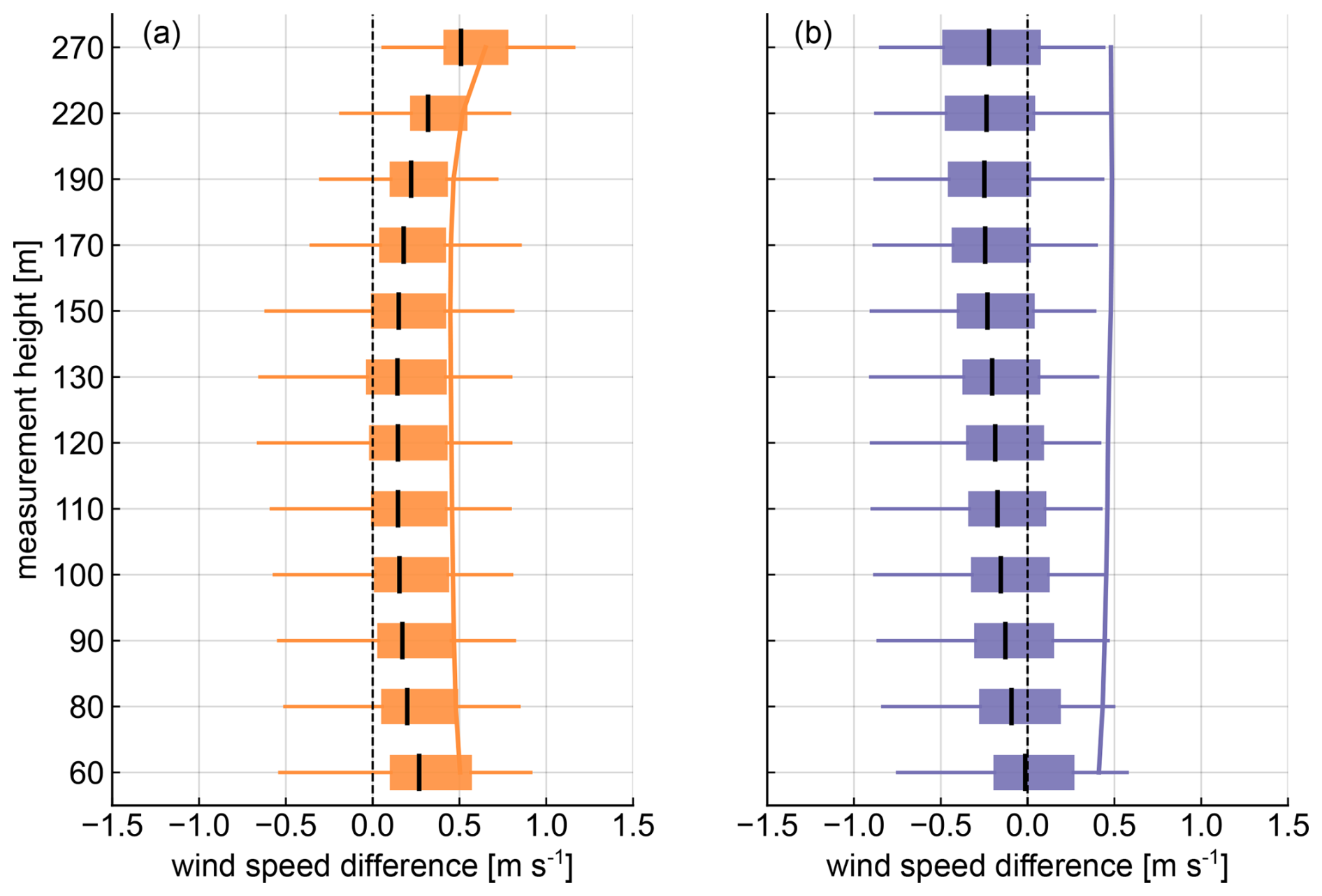
Figure 13 Box plots of the wind speed difference from ASCAT (a) and ERA5 (b) minus the lidar. The coloured boxes extend from the first to the third quartiles of the data, and the means are indicated by black lines. The whiskers extend to the data extremes, defined as a distance of 1.5 times the interquartile range (IQR) above and below the upper and lower quartiles, respectively. The solid lines indicate the RMSE between the gridded datasets and the lidar. Only grid points more than 20 km away from shore were included.

Both datasets show a comparable absolute mean in the central part of the profile, with values below ±0.2 m s⁻¹ in the height range between 90 and 170 m height. This indicates that both ERA5 and ASCAT yield similar performance in this segment of the profile, suggesting that they are both reasonably aligned with the lidar observations in the lower- to mid-altitude ranges. However, a notable difference arises when examining the overall biases. ERA5 consistently underestimates the wind speed throughout the profile, with this negative bias becoming increasingly pronounced with altitude and reaching the largest negative mean bias of around 0.2 m s⁻¹ at 270 m. Unlike ERA5, ASCAT profiles exhibit a persistent overestimation of wind speed relative to the lidar at all heights. This overestimation increases significantly above 170 m. When considering variability, as represented by the interquartile range (IQR), both datasets reveal relatively analogous patterns. For ERA5, the IQR is almost the same for all heights, with values around 0.5 m s⁻¹, suggesting that the quality of ERA5 wind speeds does not depend on height. In the case of ASCAT, the IQR displays a slight decrease with height, highlighting the larger and more consistent overestimation at higher altitudes.

The whiskers analysis provides further insight into the discrepancies between the two datasets. For ERA5, the lower whiskers extend further into negative values as altitude increases, with the larger underestimations reaching approximately −0.8 m s⁻¹ at 270 m. ASCAT's whiskers reveal a different pattern: particularly noteworthy are the upper (positive) whiskers that extend significantly beyond the lower whisker at 270 m, illustrating once again the tendency of ASCAT to overestimate wind speeds at greater heights.

The RMSE analysis corroborates the findings from the median and whisker assessments, revealing similar results for both datasets, with RMSE values around 0.5 m s⁻¹ along the profile. Nevertheless, while the RMSE remains nearly constant across the entire profile for ERA5, ASCAT's RMSE demonstrates the deteriorating performance of the employed extrapolation methodology in the upper part of the profile.

In order to evaluate the accuracy of ASCAT and ERA5 wind profiles across the different areas covered by the ship route, Fig. 14 illustrates the wind speed differences between these datasets and the lidar profiles for all grid boxes along the ship track. As can be observed, both datasets show better performance in regions located farther away from the shore, which is evident from the concentration of outliers (points falling outside the confidence intervals) in these areas. This observation holds for the three elevation levels presented. Notably, the western area of the ship route (longitude below 18.5°) exhibits the largest errors for both ASCAT-extrapolated and ERA5 winds, with maximum differences up to about 5 m s⁻¹ at all elevation levels. In the eastern area of the ship route, there are maximum differences up to 4 m s⁻¹. This indicates that wind speed estimations from these datasets are not accurate enough in coastal areas, first, due to the poor quality of ASCAT in areas closer to the coast and, second, due to the limited size of ERA5 grid boxes, which leads to an overestimation of surface roughness in nearshore areas because of land contamination. This effect is more pronounced near Nynäshamn harbour (18° E), as here, prevailing W–SW land-to-sea winds advect land roughness contamination to sea grid points, whereas at Hanko (23° E), water roughness contamination is advected to land grid points. In addition, a relatively course model like ERA5 is unable to capture the small-scale wind flow variations in these complex locations and the intricate interactions in the coastal boundary layer influenced by both land and sea.

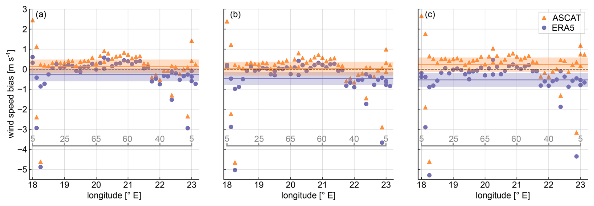
Figure 14 Wind speed bias ($\mathrm{\Delta }{U}_{\text{ASCAT}}=U_{\text{ASCAT}}-U_{\text{lidar}}$ and $\mathrm{\Delta }{U}_{\text{ERA5}}=U_{\text{ERA5}}-U_{\text{lidar}}$) along the different grid boxes depending on their longitude coordinate at 60 m (a), 150 m (b), and 220 m (c) height. The mean biases along the whole ship route are represented by solid lines, and the 95 % confidence interval is indicated by the shaded areas. The approximate distance from the centre of the grid boxes to the shore, in kilometres, is indicated by the labels of the grey line.

The mean differences vary depending on the dataset and elevation considered, highlighting the different shear exhibited by each of the datasets and their different representations of the wind profiles. ERA5 shows a smaller mean difference of −0.25 m s⁻¹ at 60 m while reaching a maximum value of −0.5 m s⁻¹ at 220 m. In the case of ASCAT, the smallest mean difference occurs at the intermediate height level, whereas the highest difference can also be found at 220 m height.

It can be seen that, although ERA5 usually underestimates the wind speed, this is more pronounced at higher elevations and within the western portion of the ship track. This height-dependent underestimation can be attributed to the presence of an internal boundary layer (IBL) that forms when the air flows from land to sea and the surface changes abruptly (Wood, 1982), such as near the Nynäshamn harbour with predominantly W–SW winds. As the IBL develops downstream from the coastline, the wind profile gradually adjusts to the lower roughness of the sea surface. However, at higher elevations, the IBL may not yet have fully developed closer to the shore, and the wind profile retains characteristics of the rougher land surface, leading to a more pronounced underestimation by ERA5 at higher altitudes. In contrast, ASCAT generally shows an overestimation compared to lidar measurements along most of the ship route, with only a few exceptions.

4 Concluding discussion

The objective of this study has been to assess the accuracy of ASCAT-derived and ERA5 wind speed profiles for characterising offshore winds at turbine operating heights in the northern Baltic Sea. Initially, ASCAT winds were compared with the ERA5 reanalysis dataset, which is frequently used as a fallback for offshore wind characterisation in the absence of in situ measurements. Subsequently, both gridded datasets were evaluated against reference in situ observations obtained from a novel ship-based lidar measurement campaign.

To extrapolate ASCAT wind data, the mean stability correction methodology formulated by Kelly and Gryning (2010) was used. This method uses the mean ASCAT wind measurements at 10 m altitude during the campaign, along with atmospheric stability information derived from ERA5. It should be noted that previous studies (Optis et al., 2021) have suggested that machine-learning-based techniques to extrapolate satellite winds could outperform the mean stability correction method used in this study. However, the limited amount of data available during the campaign period hinders the implementation of such data-driven approaches.

The collocated and full campaign strategies demonstrated remarkable agreement, with minimal differences at 100 m in the offshore areas. However, significant discrepancies were reported in coastal areas, where the collocated approach consistently exhibited lower wind speed values, with maximum differences of up to 0.4 m s⁻¹. These differences are mainly explained by the temporal discretisation of ASCAT overpasses, which influence the prevailing stability conditions captured by each approach. This is particularly noticeable near Nynäshamn harbour, where a more pronounced stability daily cycle is observed as a consequence of the coastal contamination of ERA5 grid boxes in the area and the predominant land-to-sea winds. Furthermore, the use of generic empirical constants C_±, kept uniform throughout the area, can result in inaccurate theoretical distributions in some regions. Different studies have adopted varying values of these constants based on observed stability conditions (Kelly and Gryning, 2010; Badger et al., 2016; Optis et al., 2021). Therefore, further research is necessary to establish a reliable and standardised methodology to determine the optimal values of these constants according to site-specific stability conditions.

The comparison between ASCAT and ERA5 winds reveals an overall good agreement when assessing mean wind speeds across the open-sea area of the Baltic Sea. However, ASCAT consistently reports higher wind speeds than ERA5, with a mean bias of approximately 0.45 m s⁻¹ at 10 m and 0.64 m s⁻¹ at 100 m. Greater discrepancies are observed near the coast, often exceeding 1 m s⁻¹. The mean wind speed bias decreases with increasing distance from the coast, stabilising at approximately 0.2 and 0.4 m s⁻¹ at 10 and 100 m, respectively, in grid cells beyond 40 km from the coast. The larger overestimation of ASCAT in the coastal areas of the Baltic Sea, along with the better agreement between ERA5 and ASCAT in offshore regions, has also been reported by Hasager et al. (2020). Additionally, Duncan et al. (2019a) reported an increased bias of around 0.6 m s⁻¹ in the North Sea's coastal regions. This trend can be attributed to the inherent limitations of both datasets. For ERA5, its coarse spatial resolution leads to land contamination in grill cells near the coast, overestimating the surface roughness and consequently underestimating wind speeds. Furthermore, ERA5's resolution limits its ability to simulate coastal atmospheric dynamics and small-scale wind flow variations, particularly in areas with abundant small islands and rocky islets, which are especially common in the coastal regions analysed in this study (Dörenkämper et al., 2015; Gualtieri, 2021). In contrast, ASCAT tends to overestimate wind speeds in some coastal areas, potentially due to effects such as wave breaking and surface slicks (Johannessen, 2005; Kudryavtsev, 2005) caused by the large number of small islets that result in excessively high wind field retrievals at 10 m. The application of high-resolution satellite technologies, such as SAR, could enhance the resolution of coastal wind speed gradients due to their finer grid spacing (de Montera et al., 2022). However, in this study, SAR measurements were not considered due to their lower temporal resolution compared to ASCAT and the relatively short duration of the campaign. This decision was made to maximise the amount of data collected and ensure consistency in the statistical metrics evaluated.

When comparing the overall mean wind profiles, ASCAT exhibited a closer agreement with the lidar wind profile than ERA5, particularly between 100 and 150 m. However, a closer analysis of individual locations along the ship route (A–F) reveals that this is a result of averaging profiles from nearshore and offshore sites. While the overall agreement between the three datasets is strong, with mean deviations from the lidar profile remaining below 0.6 m s⁻¹ for both datasets at the four offshore sites, ASCAT profiles at nearshore locations A and F show significant overestimations relative to lidar measurements, with mean differences of 2.5 and 1.1 m s⁻¹ at A and F, respectively. In contrast, ERA5 performs better in capturing the wind shear throughout the profile exhibiting a more consistent bias, which is in line with previous studies in the southern Baltic Sea (Rubio et al., 2022). The results also highlight a consistent underestimation of ERA5 throughout the entire profile, with a negative bias peaking at −0.2 m s⁻¹ at 270 m. Conversely, ASCAT consistently overestimates wind speeds at all altitudes, with this overestimation rapidly increasing above 170 m and peaking at around 0.5 m s⁻¹ at 270 m, as evidenced in Fig. 13. It is important to note that, unlike the MOST stability correction approach, the mean stability correction approach used here can be applied above the surface layer. The findings of this study indicate a good performance within the lower 170 m of the atmosphere. However, the applicability of this method depends on the specific atmospheric stability conditions at the location of interest and the duration of the comparison period.

The spatial evaluation of the bias of the ERA5 and ASCAT wind speeds relative to lidar measurements along the ship route reveals that both datasets perform better in far-from-shore regions, with the largest errors observed near harbour locations (longitudes further west from 18.5° E and further east from 22.5° E). Similar results were reported in Takeyama et al. (2019), where a comparison of ASCAT data and Weather Research and Forecasting (WRF) simulations against in situ measurements in the vicinity of the Japanese coast revealed significantly reduced errors beyond 25 km from the shore. In this study, the western section of the ship route shows the largest discrepancies, with differences reaching up to 5 m s⁻¹ for both datasets and across all height levels. These inaccuracies are mainly due to limited ASCAT performance near the coast and ERA5's coarse spatial resolution, which results in surface roughness overestimation caused by land contamination in nearshore grid cells. This effect is especially evident near Nynäshamn harbour, where the prevailing W–SW winds advect land influence over adjacent grid boxes. As a key difference between the two gridded datasets is their bias pattern, ERA5 generally underestimates wind speeds, especially nearshore and at higher elevations, whereas ASCAT tends to overestimate wind speeds along the entire route, with larger biases at higher altitudes too.

One distinct aspect of the ship-based lidar campaign conducted on board a ferry ship is the near-constant correlation between the ship's position and the time of day. Therefore, and similarly to the discretised temporal resolution of ASCAT observations, the derivation of a complete diurnal wind speed cycle from these measurements in the specific areas covered by the vessel route is not feasible. Consequently, the mean values derived from lidar measurements may exhibit biases that vary depending on the time slots during which measurements were acquired at particular locations. Furthermore, it is acknowledged that lidar measurements, like any other observational data, are subject to inherent uncertainties that may impact the results (Duncan et al., 2019b; Rubio and Gottschall, 2022). However, quantifying the uncertainty of ship-based lidar systems remains challenging due to their non-stationary nature, which hinders a direct comparisons with fixed reference measurements. Nonetheless, previous studies have demonstrated good agreement between ship-based lidar measurements and both FINO1 mast observations (Wolken-Möhlmann et al., 2014) and alternative data sources such as numerical models (Rubio et al., 2022) and radiosondes (Zentek et al., 2018; Zhai et al., 2018). Based on this and acknowledging that further efforts are needed to fully characterise the uncertainty of ship-mounted lidars, we assume that the uncertainty of a ship-based lidar with a motion compensation algorithm implemented is comparable to that of a buoy-based lidar system. Consequently, the observed deviations between the lidar measurements and both extrapolated ASCAT and ERA5 significantly exceed the magnitude of potential discrepancies attributable to floating lidar uncertainties, which has been reported to be approximately 3.1 %–4.2 % at 92 m height for wind speeds between 4 and 16 m s⁻¹ (Dhirendra et al., 2016).

The fundamental differences of this study from the previous literature are the comparison of ASCAT wind profiles against lidar measurements across a broad geographical domain, within an increased vertical extension and through the application of a novel collocating technique. This brings valuable revelations concerning the prospective applicability of ASCAT observations within varying spatial constraints and their feasibility at higher altitudes, including turbine operational heights.

In conclusion, extrapolated ASCAT wind retrievals using the mean stability correction approach may serve as a useful additional asset for characterising offshore winds at turbine operation heights, manifesting accuracy levels comparable to numerical model outputs from ERA5 in far-from-shore regions. This methodology is particularly beneficial in scenarios where more complex extrapolation methods are impractical or when in situ measurements are limited, providing an additional source of wind information and thereby improving the reliability of offshore wind characterisation. However, the application of both ERA5 and ASCAT must be approached with caution due to their inherent characteristics, including insufficient spatial resolution and the inability to adequately capture wind farm wake effects, which limit their utility for detailed wind farm energy yield assessments. Despite this, these datasets are still valuable for other applications, such as large-scale planning of wind potential, preliminary site screening studies that help to identify regions with promising resources, or to generate wind atlases in offshore regions through the combination of these and other datasets (Doubrawa et al., 2015). In such cases, the findings of this study provide valuable insights into the conditions under which these datasets and methodology can be applied and the level of reliability that can be expected. Nonetheless, it is crucial to also acknowledge the primary limitations of this approach, such as excessive wind speed deviations in nearshore locations and the increased expected error at higher altitudes.

Future research could explore the suitability of other satellite technologies, such as SAR measurements, with a superior spatial resolution, to mitigate the issues associated with coastal contamination. Additionally, ship-based lidar systems offer reliable wind measurements within vast areas of investigation, underscoring their potential for validating and optimising not only satellite extrapolation methodologies, as well as numerical models datasets, including regions where wind farm wake effects play a significant role.