First nationwide analysis of riming using vertical observations from the operational German C-band radar network

The 17 operational German C-band polarimetric weather radars routinely perform a vertical “birdbath” scan, which has so far primarily been used for calibration of differential moments. In this study, we transfer a retrieval algorithm for the rime fraction of snowflakes – originally developed for Ka-band cloud research radars – to the operational birdbath scan. This retrieval, which relies on the increase in detected mean Doppler velocity, serves as our benchmark. To validate the transfer of the retrieval, we apply it to a resampled birdbath dataset, constructed by downsampling cloud radar data to match the resolution of the operational birdbath scan. In addition, we present a new clutter filter and a melting layer detection algorithm for the operational birdbath scan. Finding good agreement between resampled and benchmark datasets, we apply the new retrieval to radar data recorded during the winters of 2021 to 2024. This results in a nationwide map of riming events in wintertime clouds. There is a north-south gradient in the riming distribution, which can be linked to Germany's precipitation climatology. Notably, we show that the occurrence of riming events correlates more strongly with precipitation intensity than with the total number of precipitation hours across sites. The temperature distribution associated with riming is consistently between −15 and 0 °C at all sites, except for the Feldberg site, which hints at a possible orographic effect. This study demonstrates that the operational birdbath scan of C-Band weather radars can be used for the retrieval of microphysical processes. Corresponding solutions, challenges and methods to transfer retrieval algorithms from research cloud radars to the operational weather radars are discussed.

1 Introduction

Riming refers to the collision of frozen hydrometeors – such as ice crystals or aggregates – with supercooled liquid water droplets in mixed-phase clouds. Upon impact, the droplets freeze, causing the hydrometeors to gain mass (Lasher-Trapp, 2022; Pruppacher and Klett, 1996). This process removes liquid water from the cloud and contributes efficiently to precipitation formation (Grazioli et al., 2015; Houze and Medina, 2005; DeLaFrance et al., 2024). In observations, rimed ice has been found to contribute over 50 % of snow mass (Harimaya and Sato, 1989; Mitchell et al., 1990; Borys et al., 2003; Zhang et al., 2021). However, modeling riming accurately remains challenging due to the complex phase interactions and irregular shapes of frozen hydrometeors (Leinonen and Szyrmer, 2015; DeLaFrance et al., 2024).

One of the most robust indicators of riming is an increased sedimentation velocity of the hydrometeors, resulting from their higher bulk density compared to unrimed ice crystals or aggregates. In vertically pointing radar observations, known as the “birdbath view”, this manifests as enhanced mean Doppler velocities, which can be used to classify the presence and intensity of riming (Mosimann, 1995; Kneifel and Moisseev, 2020). Strong riming typically occurs in the form of discrete events, which happen on a multi year average every fourth to fifth day and can last from several minutes to several hours (Ockenfuß et al., 2025). Therefore, short-term measurement campaigns often fail to capture a sufficient number of riming events for robust statistical analysis.

Longterm vertically pointing observations have long been a standard component in the measurement strategy of cloud research radars within radar networks like Cloudnet, where they support detailed investigations of cloud and precipitation microphysics (Illingworth et al., 2007). Therefore, they serve well to study for example, riming on a longer time scale like in Kneifel and Moisseev (2020) and Ockenfuß et al. (2025). However, as cloud research radar sites are sparse, it is difficult to assess the applicability of those results over larger areas and reveal spatial patterns.

In contrast, operational weather radars are numerous and widespread in many countries, but have historically used the birdbath scan mainly for calibration purposes (Frech et al., 2017). For example, in Germany, the national weather radar network operated by the German Meteorological Service (DWD) comprises 17 polarimetric C-band radars. While these operational radars primarily perform wide area azimuth scans (commonly referred to as plan position indicator (PPI) scans) at 10 elevations, they also include a short birdbath scan at zenith as part of their scanning routine (Frech et al., 2026). Its scientific potential remains largely untapped, with only a few recent studies beginning to explore its capabilities. For instance, Frech and Steinert (2015) analyzed a strong rain event using birdbath scan data, Gergely et al. (2025) derived hail size distributions from Doppler spectra of three hail cases, and Blanke et al. (2025) identified six cases of strong riming based on mean Doppler velocities at the Essen radar site. In general, many operational radars worldwide are capable of performing birdbath scans. For instance, the majority of the 217 radars in the European OPERA radar network (Huuskonen et al., 2014; Saltikoff et al., 2019) are already performing birdbath scans as part of their operational scanning pattern. Therefore, any analysis method, which can be transferred from the cloud research radars to the operational birdbath scan, has the potential to be applied on a large scale to much more radars and sites, than it is possible by focusing on research radars only.

In this publication, we present the first long-term scientific analysis of birdbath scan data collected from all 17 German C-band radar sites. We focus on the detection and characterization of rimed particles.

The operational C-band radar network, with its long-term, continuous measurements and equidistant spatial coverage, provides an ideal platform for investigating phenomena such as strong riming on a larger spatial and temporal scale. For the first time, it enables the study of the spatial variability of riming across a contiguous region.

This publication has two main objectives. Firstly, we develop a riming detection algorithm tailored to the C-band birdbath scan, building upon the approach presented in Ockenfuß et al. (2025) for Ka-band cloud radars. This involves two new processing components: a clutter filter and a melting layer detection algorithm specifically designed for the C-band birdbath scan. Both are computationally efficient and operate without the need for manual intervention, making them suitable for large-scale, multi-year datasets. The resulting detection algorithm enables us to quantify and compare the frequency and temperature dependence of riming across all 17 radar sites. We further relate riming frequency to local surface precipitation climatologies. Secondly, we use the riming detector for highlighting the broader challenges involved in transferring retrieval algorithms from research cloud radars to operational radar systems. We present solutions to these challenges that should be applicable beyond the specific application of riming detection.

The remainder of this publication is organized as follows: Sect. 2 describes the datasets and the methodology used to adapt the riming retrieval to the C-band radars. In Sect. 3, we first evaluate the performance of the new retrieval and then present the spatial and temporal distribution of riming across Germany. Characteristics and uncertainties of this distribution are discussed in Sect. 4. Section 5 concludes the study.

2 Methods

2.1 Benchmark Cloud Radar Riming Retrieval

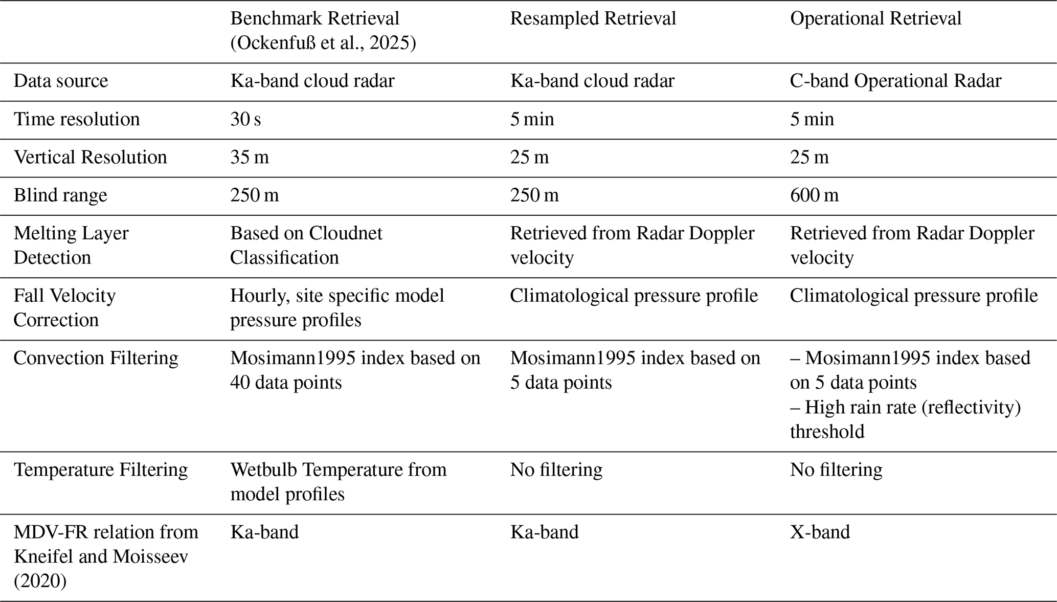
Ockenfuß et al. (2025) developed a riming detection algorithm for observations from Ka-band cloud radars like the MIRA35 35 GHz cloud radars located at the Lindenberg observatory and Jülich research site, Germany, operated by the German Meteorological Service (Görsdorf et al., 2015) and the Jülich Observatory for Cloud Evolution (Löhnert et al., 2015). The data is accessed via the Cloudnet database (Illingworth et al., 2007), with a time resolution of 30 s and a height resolution of 35 m. Their retrieval involves several filtering steps in order to separate the warm rain and ice-containing part of the cloud, based on the Cloudnet target classification (Hogan and Connor, 2004) and weather model temperature profiles. Convective regions with significant vertical air motion are excluded using a sliding window filter further discussed in Sect. 2.6. Table 1 gives an overview of those steps. Afterwards, a monotonic relation between rime mass fraction (FR) and radar Doppler velocity from Kneifel and Moisseev (2020) is applied to the ice part of the cloud. FR is defined as

$$\begin{array}{}\text{(1)}& \mathrm{FR}={\displaystyle \frac{m_{\text{r}}}{m_{\text{tot}}}}=\mathrm{1}-{\displaystyle \frac{m_{\text{us}}}{m_{\text{tot}}}}\end{array}$$

with m_tot the total mass of the particle, m_r the rime mass and m_us the mass of the unrimed snowflake or ice crystal. The minimum detectable FR with this method is 0.6, corresponding to 1.5 m s⁻¹ Doppler velocity in Ka-band radars. In a last step, nearby profiles with riming detections are clustered into connected riming events, based on a density clustering scheme described in Ockenfuß et al. (2025). In the following, we will reference the cloud radar algorithm and the corresponding results as the “benchmark retrieval” and “benchmark results”, respectively.

2.2 The operational C-Band Birdbath Scan

The German Meteorological Service (DWD) operates 17 C-band radars spread equidistantly across Germany. Their locations are depicted in Fig. 1. At each site, a birdbath scan is performed every 5 min as part of the operational scanning cycle. Originally, it was introduced to calibrate differential reflectivity ZDR (Frech and Hubbert, 2020). While the radar is oriented vertically, the dish is turning in the azimuth direction in order to smooth possible orientational effects in the radar data. The full scan takes 15 s, consisting of 15 “rays” of 1 s duration. Per ray, the radar moments are computed from a batch of 1024 pulses and stored on disk. Since July 2021, for each ray the full Doppler spectra are stored in a separate file. In the vertical, the intrinsic data resolution is 60 m, but sampling is performed at 25 m resolution (Gergely et al., 2022). In the following, we will reference the retrieval and results based upon this dataset as the “operational retrieval” and “operational results”, respectively.

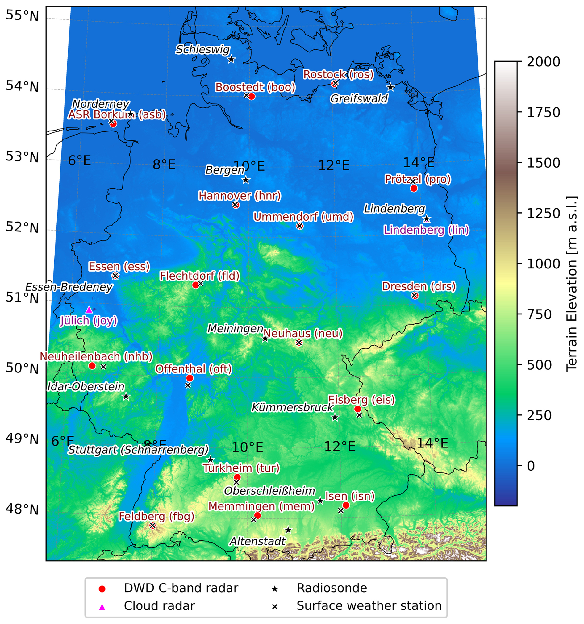
Figure 1 Overview map of Germany with locations of all measurement devices used in this publication: the 17 operational C-Band radars, the cloud radars in Lindenberg and Jülich, the sounding stations and the surface weather stations. The abbreviations for the radar sites are given in brackets behind the site name.

2.3 Retrieval Transfer

Based on our experience, when transferring any retrieval originally developed for cloud research radars to the operational C-band birdbath scan, three universal key points need to be addressed:

1. Radar band: While cloud radars typically operate in Ka-band (35 GHz) or W-band (94 GHz), the operational radars in Germany work at C-band (5 GHz). Therefore, compared to cloud radars, they are less affected by attenuation due to hydrometeors and gases. At the same time, as we show in Sect. 2.4, clutter limits the usable reflectivity range of the C-band birdbath scans to values higher than −20 dBZ, which is less than the −40 dBZ typically obtained by vertically looking cloud radars. As a consequence, for example low reflectivity cloud tops are not visible in the C-band birdbath scan (Frech et al., 2026). The same is true for liquid water peaks around 0 m s⁻¹ fall velocity in the Doppler spectra (Gergely et al., 2022).

2. Time resolution: The vertical resolution of 25 m of the C-band radar is comparable to the typical resolution of 30 to 40 m of Ka-band radars in the Cloudnet database, but the time resolution of one scan every 5 min is much coarser than typical cloud radar sampling rates. In Cloudnet categorize data, cloud radar data has a time resolution of 30 s. Therefore, all operations which act along the time dimension must be reevaluated and retuned when applied to C-band birdbath data. This affects common operations like e.g. time domain filters, fallstreak tracking (Kalesse et al., 2016) or eddy dissipation rate retrievals (Borque et al., 2016).

3. Additional data: Most modern retrieval techniques depend on more than just radar data. Surface weather stations, equipped with standard meteorological instrumentation, can provide information about the local weather conditions and the local climatology. Additional active and passive remote sensing instruments like lidars or microwave radiometers can complement radar observations, e.g. to detect liquid layers in mixed-phase clouds. High resolution model profiles are helpful for cross-checking and interpreting measurement results. For most research sites in Cloudnet, those data sources are available, but currently there is almost no additional instrumentation at the DWD C-band radar stations. Even vertically resolved model profiles are scarce. Model reanalysis datasets like ERA5 (Hersbach et al., 2020) are usually stored in a way which favors spatial analysis over the download of long, single-location time series, which would be required to complement birdbath observations.

Different strategies can be applied to overcome these issues.

Point one, the difference in radar frequency, is difficult to generalize. In our case, it is addressed by simulations for different wavelengths from Kneifel and Moisseev (2020). They simulated FR-MDV relationships for the X-, Ka- and W-band (corresponding to 10, 35 and 94 GHz, respectively). Differences between those simulations arise if some hydrometeors within the measurement volume are large enough to exhibit Rayleigh scattering in one band and Mie scattering in another band. However, for the combination of X- and C-band, this transition size is above 1 cm and Rayleigh scattering can be assumed for both bands (Matrosov, 1992). Therefore, we use their X-band relation here for the C-band.

To quantify the influence of point two, the difference in resolution, we create a resampled Ka-band radar dataset. As listed in Table 1, this dataset is created from the cloud radar data by taking only every 10th profile and upsampling the vertical to the same height levels as the operational C-band birdbath scan. Upsampling is done using linear interpolation. Comparing the results of filters and algorithms on the resampled dataset with the results from the benchmark retrieval, we can asses if they are directly transferable or need readjustment. We will use this strategy for the convection filtering (Sect. 2.6) and event detection (Sect. 3.1) part of the retrieval.

For the last point, some of the external information can be derived from the radar, e.g. the melting layer height (Sect. 2.5). In other cases, climatologies can replace local measurements, e.g. in case of the pressure profile (Sect. 2.7).

Ockenfuß et al., 2025Kneifel and Moisseev (2020)

Table 1 Comparison of retrieval configurations for the “benchmark”, “resampled” and “operational” retrieval.

2.4 Clutter Filter

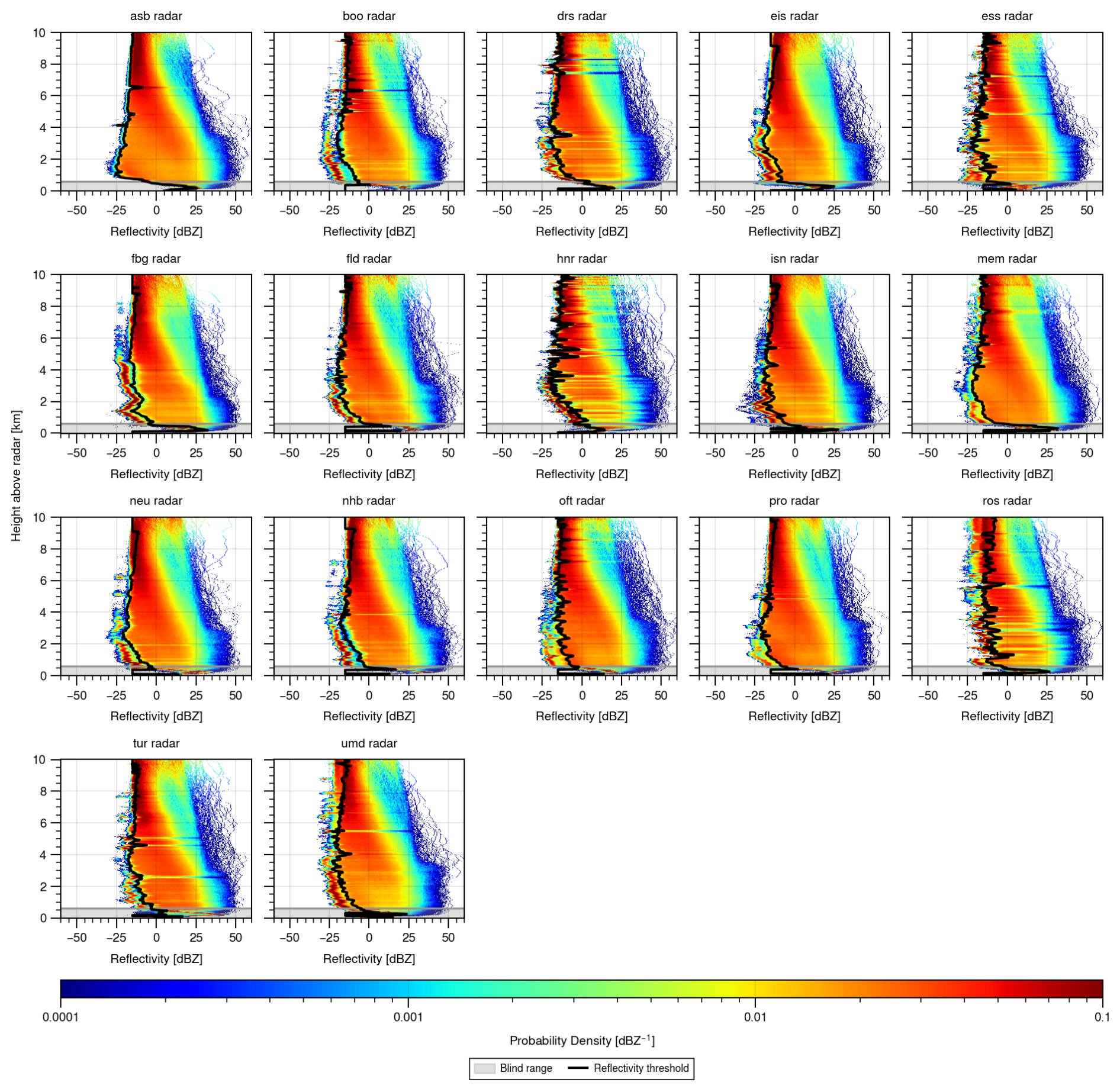
When looking slant, the sensitivity of the operational radars is −36 dB at 1 km range. For the birdbath observations, such sensitivities can not be achieved, since clutter echos dominate over weakly reflecting meteorological targets. These clutter signals are created when antenna sidelobes hit surrounding ground targets. In the radar signal processor, each range gate is quality controlled using thresholds for the noise (−9 dB), the clutter power (−25 dB) and the cross polar correlation coefficient (0.45). This thresholding is applied to all unfiltered moments in every range gate of the 15 rays. Figure 2a shows only the “valid” observations, i.e. the observations where all 15 contributing samples passed the quality control. As is evident from the horizontal clutter lines in the scene, the signal processor filtering is not sufficient. The number and height of the clutter lines varies for each radar site, depending on the ground targets in the surrounding of the radar. The reflectivity of the lines is usually between −20 to −10 dBZ. In the 2D reflectivity histogram in Fig. 2c, the clutter is visible in the form of distinct patterns at the lower reflectivity edge. In order to remove the clutter, while keeping as much of the weather signal as possible, a height and site dependent reflectivity threshold filter was developed. It makes use of the fact that every birdbath observation consists of 15 independently stored samples. For every height level, we determine the typical reflectivity of the “invalid” observations, i.e. the observations where the signal processor flagged at least one ray as invalid, based on the criteria described above. Specifically, we take the upper 5 % reflectivity quantile of all invalid observations. We then apply this reflectivity as a threshold to the valid observations. From Fig. 2c, it is evident that the height dependent reflectivity threshold is able to separate the clutter and weather parts in the histogram well for most of the height range. It can be seen that with this filtering, depending on the clutter structure, the operational birdbath scan can detect weather signals down to −20 dBZ in a range from around 1 to 10 km above the radar. The example scene after discarding the clutter part from the histogram can be seen in Fig. 2b. Since the lowest range bins are almost always dominated by strong clutter, we define a minimum valid range of 600 m at all radar sites. Compared to other methods for clutter filtering, e.g. the method presented by Gergely et al. (2022) based on Doppler spectra, our method requires no human judgement and has very low computational cost. Therefore, it is well suited to filter multiple years of radar moments from all 17 German radar sites.

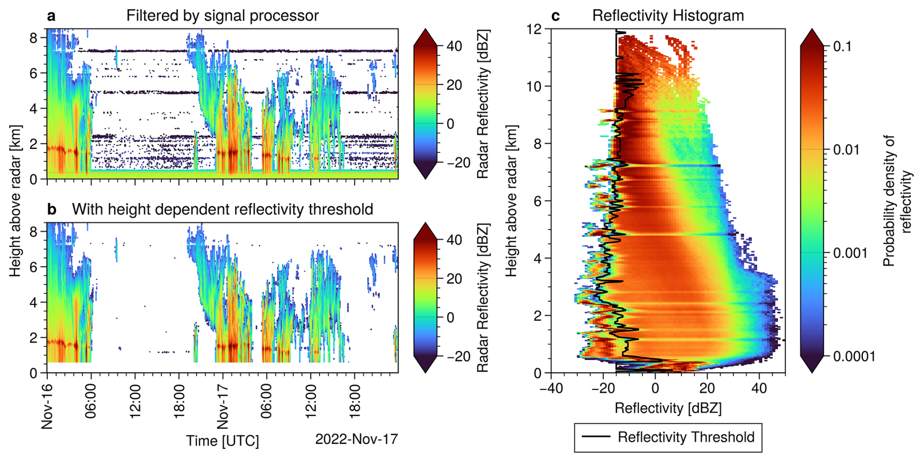
Figure 2 (a) Example of a raw measurement at the Essen radar site, with only basic filtering by signal processor. (b) The same scene after clutter filtering, where the clutter is removed based on a height dependent reflectivity threshold. (c) 2D reflectivity by altitude histogram. The clutter lines are visible as horizontal stripes in the histogram. The black line indicates the height dependent reflectivity threshold.

2.5 Melting Layer Detection

In order to detect rimed particles in the ice-containing part of the cloud, a reliable melting layer detection is necessary. In the cloud radar retrieval, this was achieved based on the Cloudnet target categorization (Hogan and Connor, 2004) and vertical temperature profiles from model reanalysis. The Cloudnet melting layer detection algorithm uses a combination of radar linear depolarization ratio (LDR), MDV and wetbulb temperature. Since neither LDR nor model profiles are available for the C-band radar sites, we need to derive the melting layer differently. For our task, the retrieval needs to work robustly on multiple sites, ideally without site-specific retuning of parameters. We do not require meter accuracy, but we want to avoid severe misdetections, where the melting layer is placed too low into the warm part of the cloud. Due to the high velocities of rain drops, those cases would falsely be detected as riming. Since actual strong riming is comparably rare, this would bias the frequency statistics of riming events.

Usually, melting layer detection is done by detecting peaks in the vertical profiles of radar moments, e.g. radar reflectivity and correlation coefficient as in Sanchez-Rivas and Rico-Ramirez (2021). In our case, we use Doppler velocity as the basis for the retrieval. Doppler velocity is unaffected by attenuation, can be measured with high accuracy and has a direct physical interpretation with high velocities in the rain part (usually >2 m s⁻¹) and lower in the ice part (<3 m s⁻¹), even in the presence of strong riming. Additionally, it allows us to apply the retrieval with the same parameters to real C-band data and the resampled dataset based on Ka-band data.

From the example in Fig. 3a, we see that in Doppler images, the melting layer is characterized by two properties:

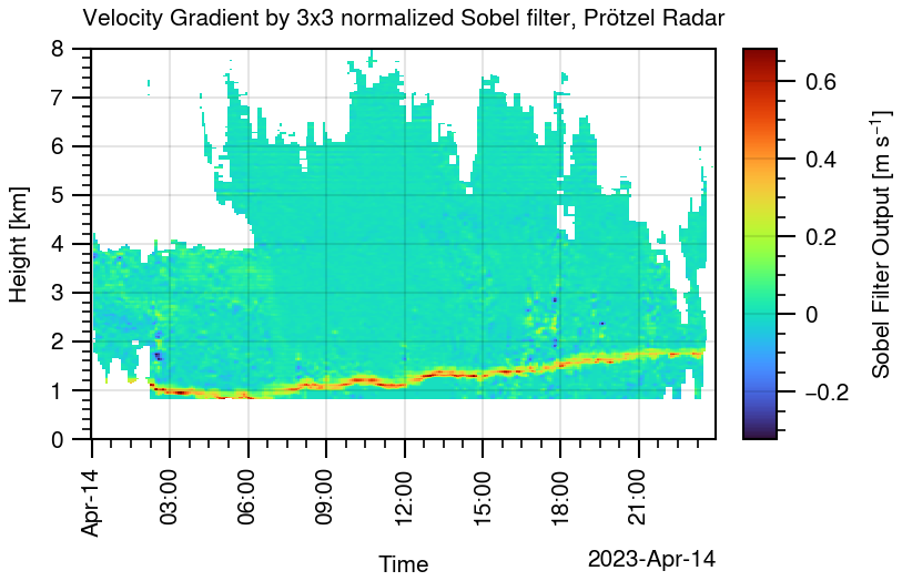
• A sudden increase in fall velocity towards the ground: As in Sanchez-Rivas and Rico-Ramirez (2021), we search for maxima in the vertical gradient ∂_hV(h) of Doppler velocity V(h), but we use the 3×3 Sobel filter presented in Wolfensberger et al. (2015) to calculate the gradients. From manual analysis, we found $\mathrm{0.2}\mathrm{m}{\mathrm{s}}^{-\mathrm{1}}{\mathrm{m}}^{-\mathrm{1}}$ to be a good gradient threshold for potential locations of the melting layer (Fig. B1 shows the gradient for the example given in Fig. 3a).

• Faster fallspeeds below the melting layer than above: Usually, the melting layer separates the Doppler image clearly into a slow and fast falling part (compare Fig. 3a). Therefore, we propose the difference in average velocities Δ_hV(h) below and above the potential melting layer as a novel, additional criterion:

  $$\begin{array}{}\text{(2)}& {\mathrm{\Delta }}_{h}V\left(h\right)={\displaystyle \frac{\mathrm{1}}{h}}\underset{\mathrm{0}}{\overset{h}{\int }}V\left(x\right)\mathrm{d}x-{\displaystyle \frac{\mathrm{1}}{H-h}}\underset{h}{\overset{H}{\int }}V\left(x\right)\mathrm{d}x\end{array}$$

  here, h is the position along the vertical and the cloud extends from height 0 to H. This concept is illustrated in Fig. 3b.

The melting layer is determined as the level with the maximum gradient ∂_hV(h), weighted by Δ_hV(h):

$$\begin{array}{}\text{(3)}& h_{\text{meltinglayer}}=\underset{h}{\arg max}\left({\partial }_{h}V\right(h)\cdot {\mathrm{\Delta }}_{h}V(h\left)\right)\end{array}$$

Including Δ_hV(h) brings information about the full column into the retrieval, instead of looking only at localized gradients. This makes it much less likely that a sudden, local fluctuation in Doppler velocity, e.g. due to riming or cloud top turbulence, is misinterpreted as the melting layer. For our application, no retrieved melting level is better than a wrong melting level. Therefore, in a postprocessing step, we remove all points where the melting layer appears to be changing by more than 300 m per 5 min. In Fig. 3c, we compare with the radar derived melting layer with the melting layer from radiosonde measurements at the Essen site, where a sounding station directly next to the radar performs two soundings per day. We define the radiosonde melting layer as the highest level, where the radiosonde crosses a zero degree isotherm of wetbulb temperature. Wetbulb temperature is calculated from radiosonde pressure, temperature and relative humidity using Normand's method (Knox et al., 2017). We see that the retrieved melting level follows the radiosonde melting layer very consistently with an offset of 200 m (±50 m). Such an offset is to be expected, since, depending on the humidity, snowflakes can sustain positive temperatures up to +4 °C on average (Heymsfield et al., 2021). In Fig. 3c, only winter months (November to April) are taken into account, and only cases where a melting level was detected in the radar as well as in the radiosonde within less than 1 h. For the riming detection, we rely on the radar derived melting layer (plus 200 m) whenever possible. Only if no reliable detection was possible, we extrapolate the last value up to 1 h and otherwise use the value from the nearest sounding station as a proxy. In the latter case, at most 12 h are tolerated between sounding and radar profile.

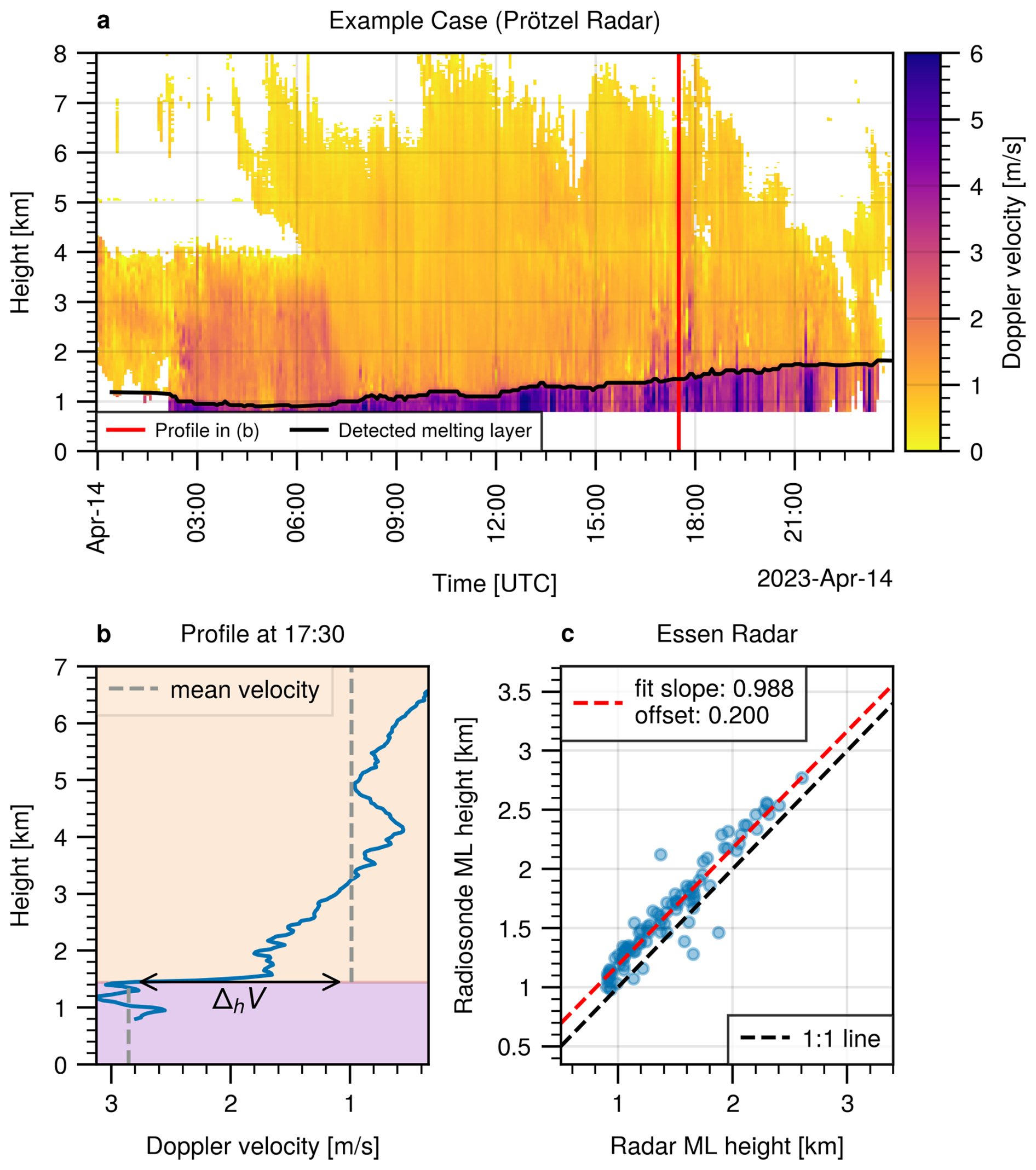
Figure 3 (a) Example of a large scale, precipitating system with signatures of riming embedded. The black line denotes the detected melting layer, the red line shows the time of the profile in panel (b). (b) Example of a vertical profile of mean Doppler velocity. The background colors separate the image in two parts, maximizing the difference in average Doppler velocity between the parts. (c) Comparison of the radar derived melting layer with the radiosonde derived melting layer at the Essen radar site. Data for the winter half of the year (November to April).

2.6 Convection Filtering

For microphysical retrievals based on MDV, one has to make sure that the signal variability is dominated by cloud microphysics and not vertical air motions. To solve this problem, we introduce two different filters based on Doppler velocity and reflectivity, respectively. Additionally, while those filters may permit to apply the retrieval all year round, for the later analysis, we focus on the winter months between November and April. In this time range, thunderstorms are highly unlikely to occur in Germany (Taszarek et al., 2019). In order to detect convective areas and regions with wave activity in clouds, Mosimann (1995) proposed the so-called convection index κ. The convection index is essentially the statistical coefficient of variation (standard deviation divided by mean) of MDV.

$$\begin{array}{}\text{(4)}& \mathit{\kappa }={\displaystyle \frac{\mathrm{|}\text{MDV}\left(z\right)-\stackrel{\mathrm{‾}}{\text{MDV}\left(z\right)}\mathrm{|}}{\stackrel{\mathrm{‾}}{\text{MDV}\left(z\right)}}}\end{array}$$

$\stackrel{\mathrm{‾}}{\text{MDV}\left(z\right)}$ is the average MDV in a ±10 min rolling window. It is assumed that positive MDV indicates downward motion. Mosimann (1995) established $\mathrm{0}<\mathit{\kappa }<\mathrm{0.2}$ as reasonable thresholds. Values beyond 0.2 are excluded as too convective situations, similarly for values below 0 indicating net upward motion. Kneifel and Moisseev (2020) and Ockenfuß et al. (2025) have confirmed this choice of parameters. However, the validity was only tested for cloud radar data with a sampling rate of 30 s or better, which yields at least 40 samples in a 20 min window. The applicability of this method to C-band radar data with 5 min resolution needs to be proven. Therefore, in Fig. 4, we compare the results of the convection filter applied to a summer precipitation event. Figure 4a is based on cloud radar data in the 30 s resolution of the Cloudnet categorize data, Fig. 4b shows the same event as resampled dataset with 5 min resolution. In the latter case, a 20 min interval contains only 5 values (including the interval edges). Nevertheless the agreement with the original filter is remarkable. In both cases, the filter is able to separate the convective beginning of the precipitation system from the stratiform trailing precipitation well. In a postprocessing step, we smooth the new filter results by removing small non-convective patches in large convective regions and vice versa. Figure 4c directly compares the two filter masks, revealing an agreement of 92 %. We also systematically tested different window sizes between 10 and 40 min and different upper κ thresholds between 0.1 and 0.4, but found the best agreement (i.e. highest overlap) by keeping the original (20 min and 0.2) parameters.

With actual C-band data, there are new, additional ways to detect heavy convection. Ka-band cloud radars usually do not detect reflectivities beyond 30 to 40 dBZ due to receiver saturation and attenuation. The C-band weather radars are weakly affected by attenuation and can record reflectivites up to 65 dBZ all along the profile in heavy summer precipitation. Therefore, we search for reflectivities beyond 35 dBZ below the melting layer, which is a common threshold to identify convective cells (Jung and Lee, 2015; Muñoz et al., 2018). If such values occur together with absolute Doppler velocities exceeding 5 m s⁻¹ above the melting layer, this is a sign of convective cells with severe vertical air motion. Since there can be a time offset between the occurence of high up and downdrafts and heavy precipitation at the ground, we add a margin of 1 h and exclude such intervals completely from further analysis. Figure 5a illustrates such a convective case, where those criteria lead to the exclusion of the time range marked in red. On average, about 7 convective events are excluded due to high reflectivity per radar for the winters 2021 to 2025. Including the margin, this amounts to 9 h of observations or 0.6 ‰ of the total observations.

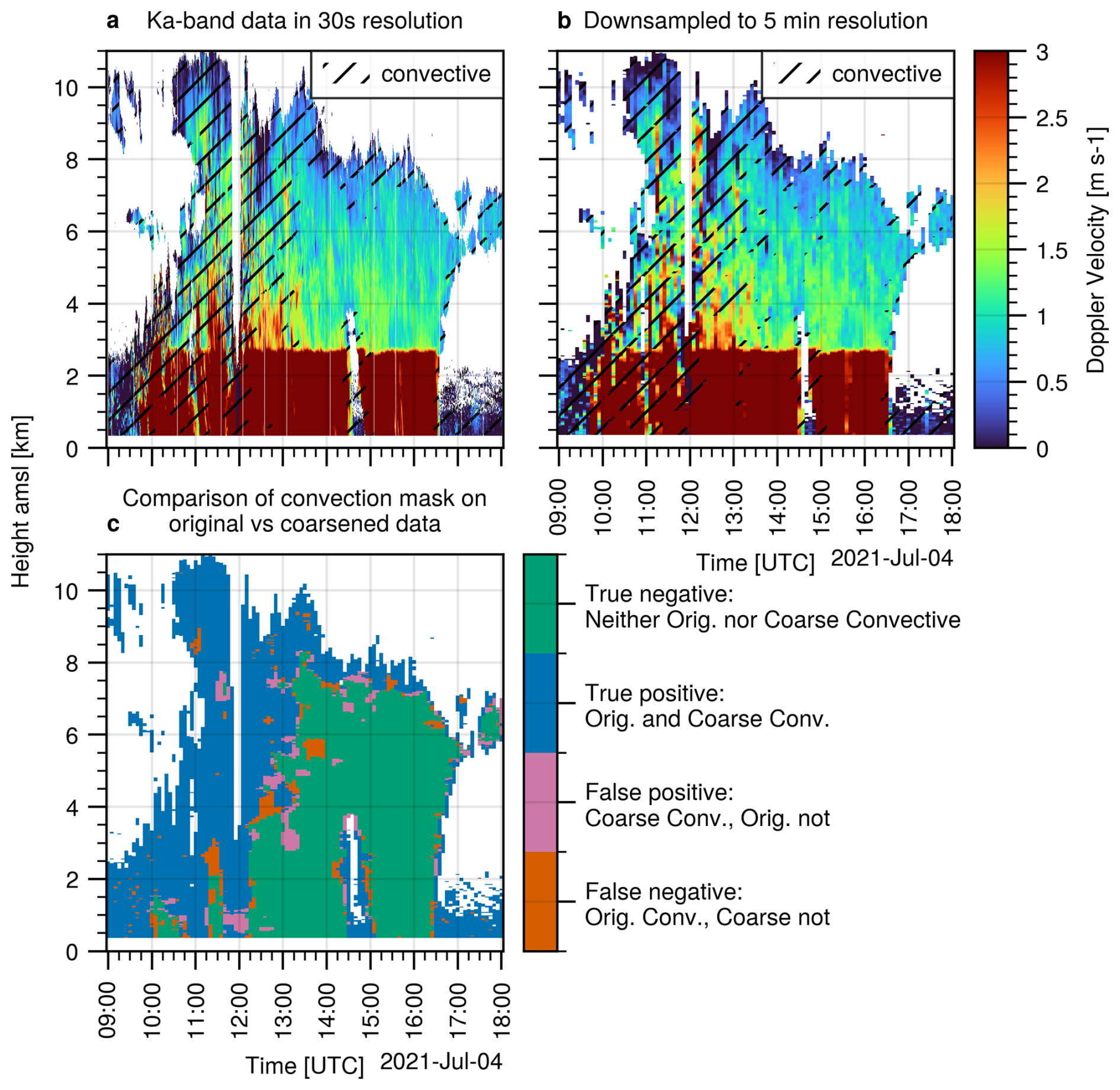
Figure 4 (a) The Mosimann convection filter applied to a summer precipitation event in the original 30 s resolution. (b) Convection filter applied to the event from (a) in 5 min resolution. (c) Comparison of the filtered areas in (a) and (b).

2.7 Fall Velocity Pressure Correction

Since the MDV-FR relation by Kneifel and Moisseev (2020) is valid for 1000 hPa ambient pressure, it is necessary to correct the fall velocities for the decreasing pressure higher in the atmosphere. Kneifel and Moisseev (2020) proposed the parameterization by Heymsfield et al. (2013):

$$\begin{array}{}\text{(5)}& {\displaystyle }{\text{MDV}}_{\text{surface}}=\text{MDV}\times \mathit{\eta }\text{(6)}& {\displaystyle }\mathit{\eta }={\left({\displaystyle \frac{p}{p_{\text{surface}}}}\right)}^{\mathrm{0.4}}\end{array}$$

For the pressure profile, Ockenfuß et al. (2025) used hourly profiles from numerical weather models. In Blanke et al. (2025), collocated radiosonde soundings were used for this task. For the 17 C-band sites, neither model nor radiosondes are directly available at all sites. However, we argue that the site and time specific pressure profiles can be replaced by a generic climatological profile. Figure 5b shows the variability σ_η of η for different heights, relative to the climatological mean.

$$\begin{array}{}\text{(7)}& {\mathit{\sigma }}_{\mathit{\eta }}={\displaystyle \frac{\mathit{\eta }-<\mathit{\eta }>}{<\mathit{\eta }>}}\end{array}$$

$<\mathit{\eta }>$ denotes the climatological average over 20 000 soundings from the Lindenberg observatory between the years 2010 to 2024. As is evident, the error in η by neglecting the temporal variability in atmospheric pressure is below 1 % for almost all cases within the typical height ranges of riming (0 to 6 km). This error is smaller than the uncertainty inherent in the MDV-FR relation due to the variability of the underlying measurements by Kneifel and Moisseev (2020), and can therefore be neglected.

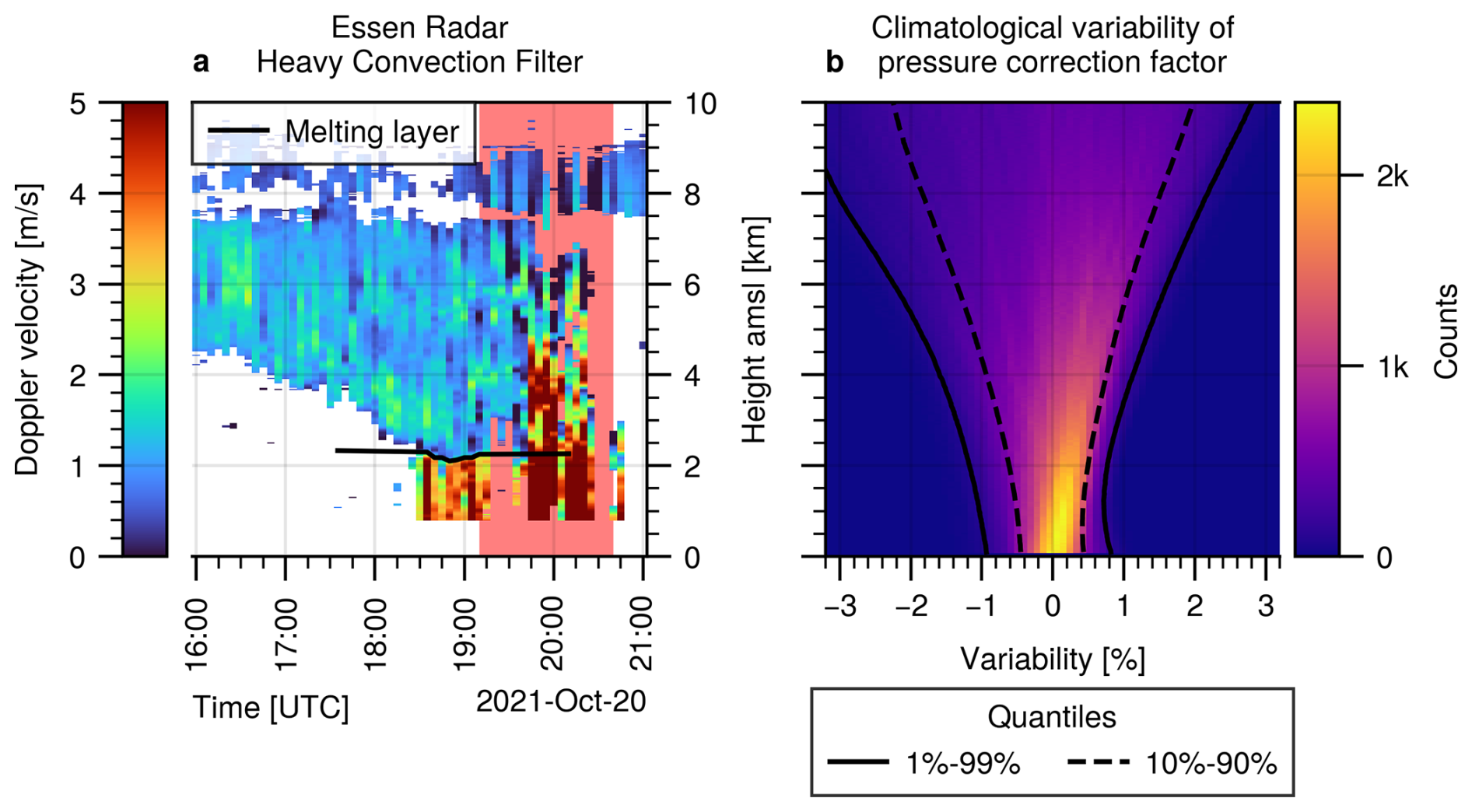
Figure 5 (a) Example of a convective event at the Essen radar site. The red time interval is excluded from any analysis due to the high reflectivites in the liquid part and the high Doppler velocities in the ice part of the cloud. The black line shows the extrapolated melting layer, detected by the method described in Sect. 2.5. (b) Relative variability of the pressure correction factor due to natural pressure variability.

2.8 Clustering

The time intervals where rimed particles are detected are then clustered into riming events. For this step, we use the same definitions and parameters as in Ockenfuß et al. (2025). They define a riming event as the maximum time interval, in which at least 75 % of the birdbath profiles show riming in at least one range gate. Events covering less than 2 min × km in the time-height image (equal to 17 pixels) are discarded, since they can be likely caused by a few noisy observation pixels with enhanced Doppler velocity. This threshold is consistent with filters applied by Kneifel and Moisseev (2020) and Ockenfuß et al. (2025).

2.9 Histogram Correction

In order to compare the temperature distribution of riming events between different radar sites in Sect. 3.4, we need to correct the distributions for deviations due to the following three points:

1. Differences in the radar uptime: Due to technical problems or maintenance, the total number of available observations varies. Radars with less uptime naturally detect less riming cases.

2. Differences in radar elevation: Radars located at higher elevations detect less riming at warmer temperatures than radars at lower elevations, since higher elevation radars can only observe the upper part of the atmosphere.

3. Differences in riming climatology: There are natural differences in the total number of riming detections between the sites. Those differences will be analyzed in detail in Sect. 3.3. We will correct for them for the temperature analysis in Sect. 3.4.

In order to correct for the points above, we count how often a certain isotherm is observable for each radar, taking into account the radar elevation and blind range. The isotherm information is again taken from the closest radiosonde to each radar site. We require less than 12 h difference between radar and radiosonde observations. Figure 6 shows an example of the number of observations per isotherm for the Feldberg, Memmingen and Isen sites during winter (November to April). We clearly see that the Memmingen radar had a longer maintenance period and therefore less observations in total. We also see that the Feldberg radar is located at a higher elevation and therefore, there are less observations at warmer temperatures compared to the Isen radar. For the results in Sect. 3.4, we divide the absolute number of riming detections per radar and temperature level by the curves in Fig. 6. This corrects for the points 1 and 2. Then, normalizing the resulting distributions to have an area of one under the curve corrects for point 3.

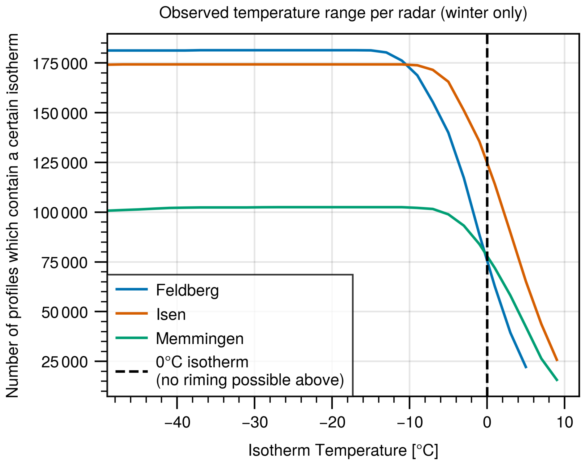
Figure 6 Number of observations per isotherm for three selected radars to illustrate the effects of radar uptime and altitude.

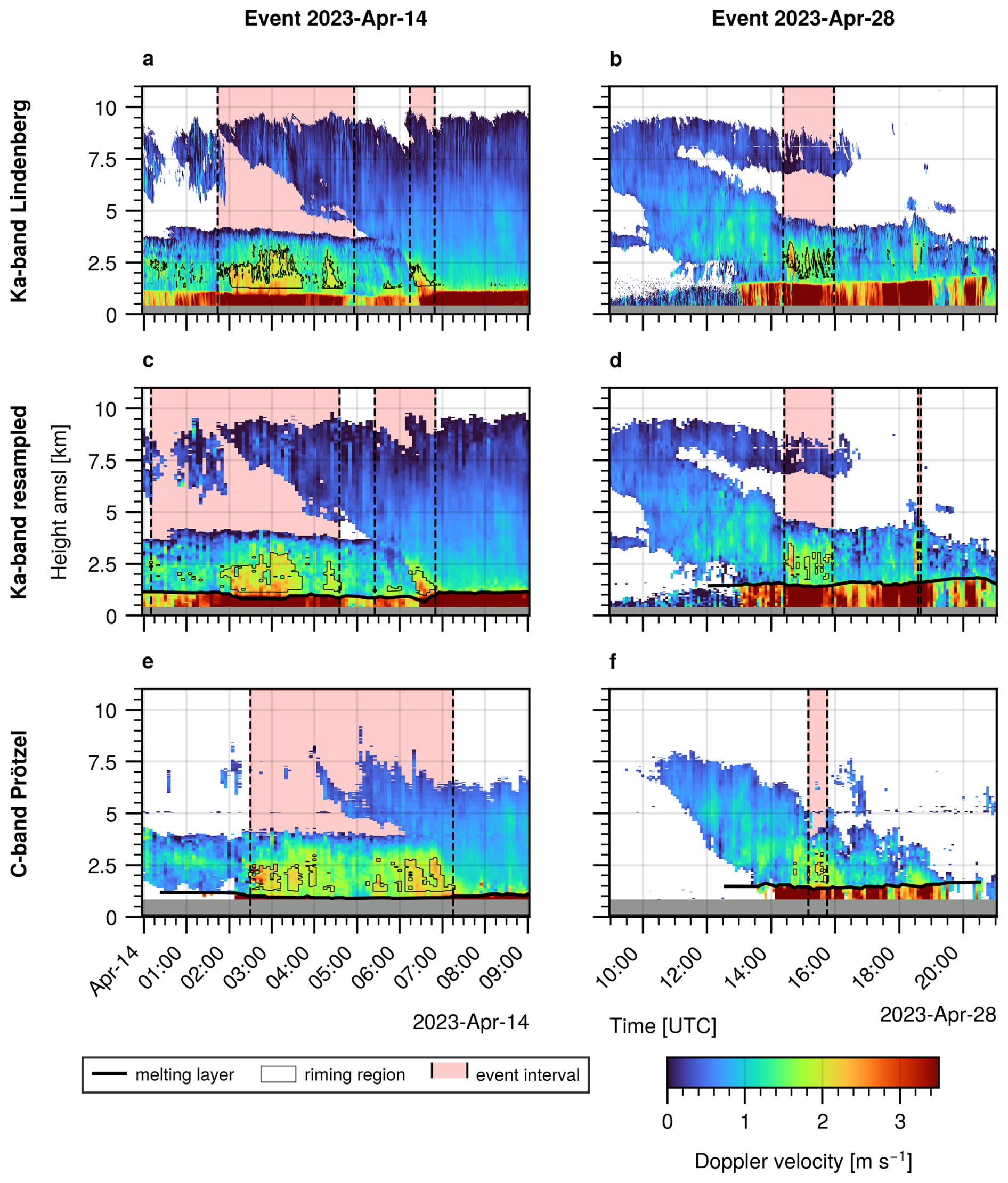
Figure 7 Examples of two events with riming signatures. Left column: 14 April 2023. Right column: 28 April 2023. (a, b) Observations by the Lindenberg cloud radar in 30 s resolution, with riming regions detected by the benchmark retrieval. (c, d) Resampled Ka-band radar data in 5 min resolution, based on the data from row one. Riming regions detected by the retrieval on the resampled dataset. (e, f) C-band radar data in 5 min resolution from the Prötzel radar site. Riming regions detected by the operational retrieval.

3 Results

3.1 Comparison with Resampled Data

Figure 7 a and b show two examples of stratiform, frontal systems with embedded riming, as well as the detected riming regions and the event clustering by the benchmark retrieval. The first example is a widespread precipitation system passing over Germany from the Southeast. This synoptic situation is often associated with intense precipitation. In this case, we see very strong riming signatures over an extended period of time. The second example also depicts a frontal passing, but with smaller riming cells, more typical for the majority of events. Figure 7c and d show the resampled version of the cloud radar measurements in Fig. 7a and b. As we can see, the large scale features of the cloud system are preserved well even with only 5 min resolution. In general, the newly developed retrieval applied to the resampled Ka-band data is able to highlight the same regions within the cloud as the benchmark retrieval. For some cases, the change in resolution leads to a different, but still reasonable, choice of the event clustering algorithm.

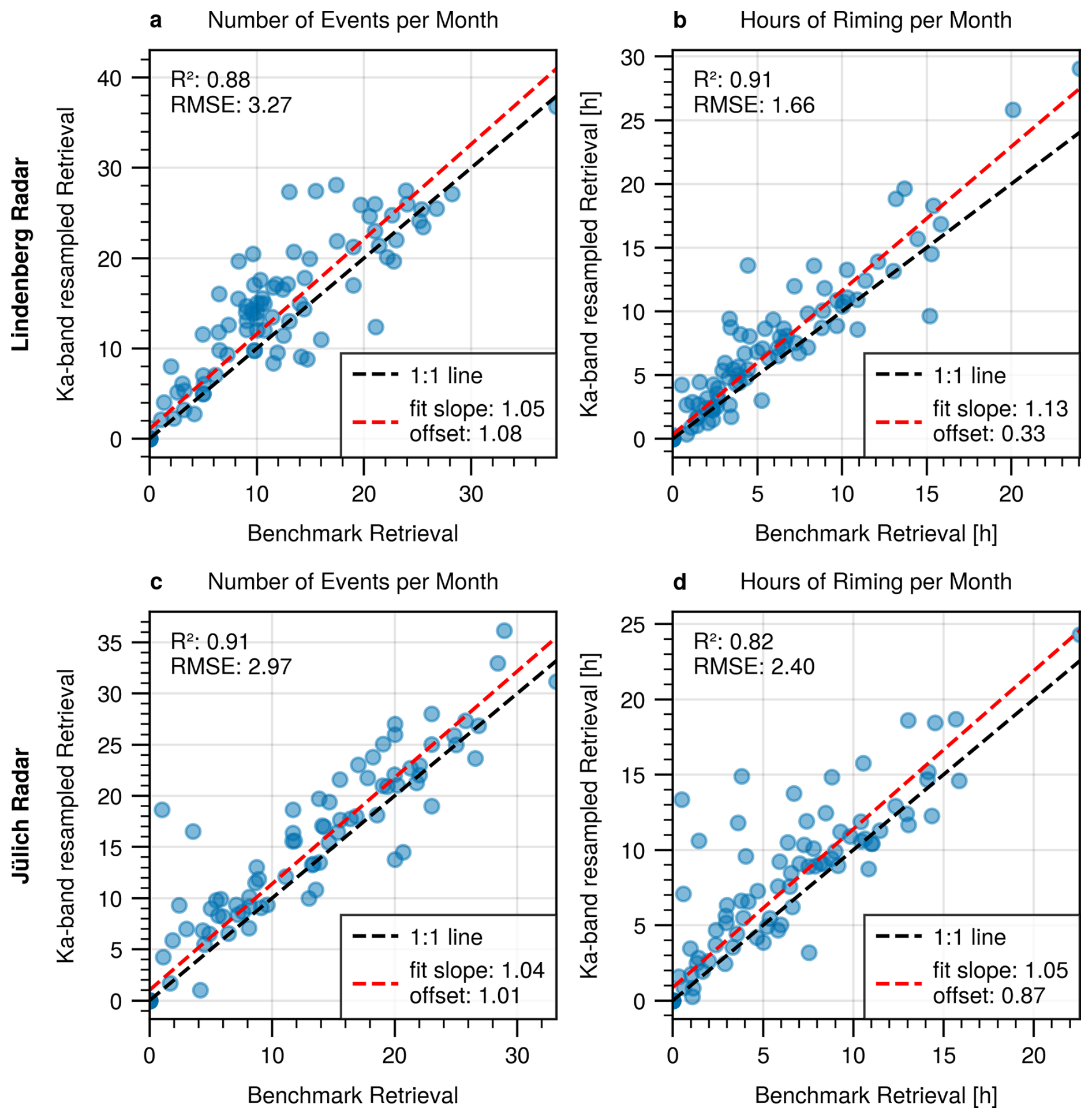
Figure 8 (a) Monthly number of riming events detected by the Lindenberg benchmark and resampled retrieval. (b) Same as (a), but for the total monthly duration of riming. (c) Same as (a), but for Jülich and Essen. (d) Same as (b), but for Jülich and Essen.

Figure 8 compares the benchmark and resampled retrieval statistically with respect to the monthly number of events (Fig. 8a, c) and the monthly duration (Fig. 8b, d). We see that the resampled retrieval can produce slightly different results for some months, but the overall correlation between both retrievals is good for both investigated sites. On average, the resampled retrieval seems to detect a little bit more/longer riming events per month, as is evident from the red fit line being above the black 1:1 line. From manual inspection, we found multiple reasons for this: Sometimes, as for example in Fig. 7a and c or Fig. 7b and d, the clustering can be different. In some other cases, the retrieved melting layer can be too low, causing rare false positives due to rain being classified as riming. Overall, we conclude that the changes we introduced in resolution, filtering and melting layer retrieval (see Table 1) should not bias riming statistics significantly.

3.2 Comparison with C-band data

In Fig. 7e and f, we see the actual C-band measurements at the same time as the cloud radar measurements in Fig. 7a and b. When comparing the two scenes, we have to keep in mind the 52 km distance between the radars. As expected due to the lower sensitivity of around −15 to −20 dBZ, the C-band radar is lacking the cloud tops between 7 and 10 km height. The same is true for periods with weak rain or drizzle below the melting layer. It is remarkable that in these cases, the C-band riming retrieval highlights similar time periods and regions in the cloud as the cloud radar algorithm. This supports the findings in Ockenfuß et al. (2025), that some riming events in stratiform systems can cover extended areas. Based on the duration and wind advection, they estimate a median extent of at least 13 km and around 10 % of the events to extend over more than 50 km radius.

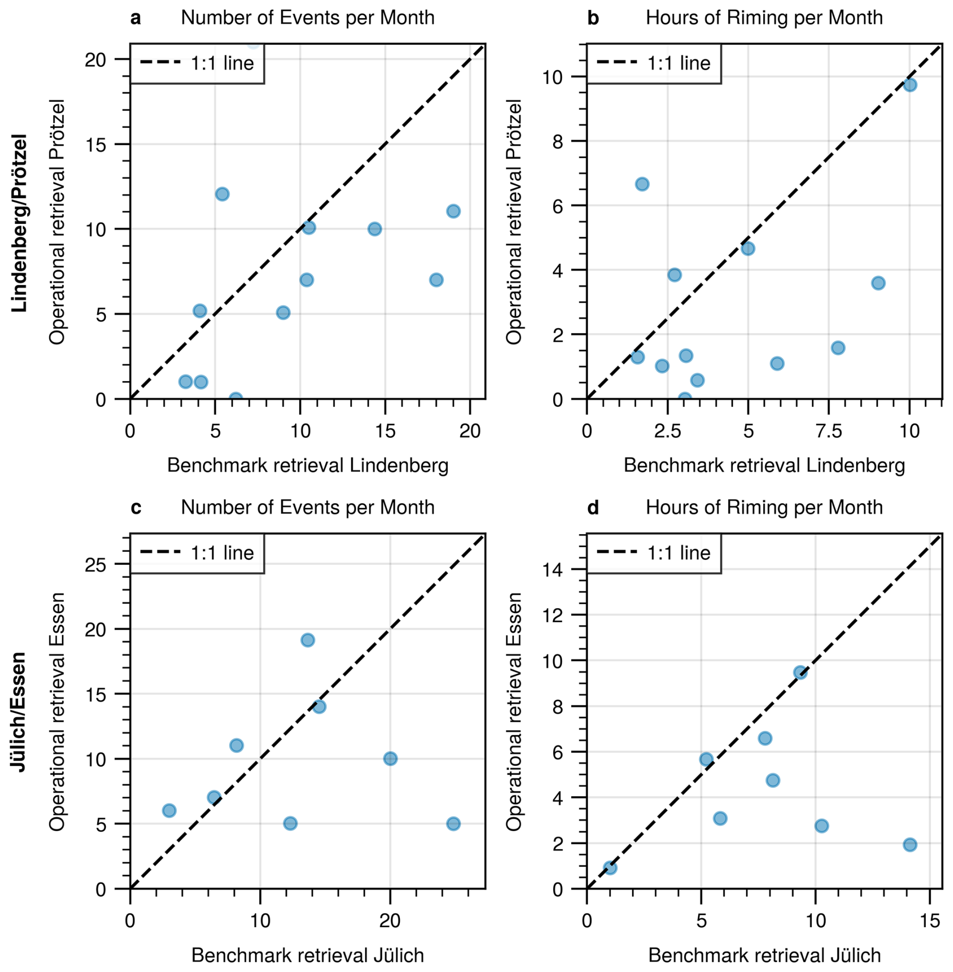
Figure 9 (a) Monthly number of riming events detected by the Lindenberg benchmark and Prötzel operational retrieval. (b) Same as (a), but for the total monthly duration of riming. (c) Same as (a), but for Jülich and Essen. (d) Same as (b), but for Jülich and Essen. The different number of samples between (a, b) and (c, d) is due to differences in radar uptime.

However, these findings also imply that we cannot expect a direct correlation between the time series recorded by the cloud radar and C-band radar, given the 52 km (68 km for Jülich-Essen) distance separating them. This limitation is clearly illustrated in Fig. 9, which aggregates data from 12 winter months between November 2021 and April 2023. On a monthly scale, we observe only a weak correlation between the two retrievals and sites. The natural variability in cloud and precipitation structure across the sites introduces considerable scatter around the 1:1 line – much more than what is seen in Fig. 8.

Consequently, meaningful comparisons between the two retrievals can only be made on the basis of long-term climatological statistics. When comparing the total number of riming events detected over the 14-month period and correcting by differences in radar uptime, the C-band radar Prötzel identifies 26 % fewer events than the cloud radar Lindenberg (30 % for Jülich-Essen).

From the previous experiments with the resampled dataset, we know that this discrepancy cannot be attributed to the lower temporal resolution of the C-band measurements or to any changes in the retrieval algorithm. Instead, the reduced detection rate must be inherent to the C-band system itself. Especially two properties may be important: Its lower sensitivity, around −15 to −20 dBZ, makes it less capable of detecting riming in low-reflectivity mixed-phase clouds that occur during the cold season. In addition, the larger blind range of 600 m further limits the detectability of events close to the radar. We can quantify the relative importance from sensitivity and blind range by introducing a similar 600 m blind range and sensitivity to the cloud radar data. If the blind range is introduced, the discrepancy in event counts is reduced to 19 % (26 % for Jülich-Essen). For the sensitivity, we introduce a −17 dBZ detection limit to the resampled Ka-band dataset, consistent with the average sensitivity of the Essen and Prötzel C-band radars in the 0 to 5 km height region. For the Lindenberg-Prötzel comparison, this has no significant effect. For the Jülich-Essen case, 3 events are discarded, reducing the spread to 24 %.

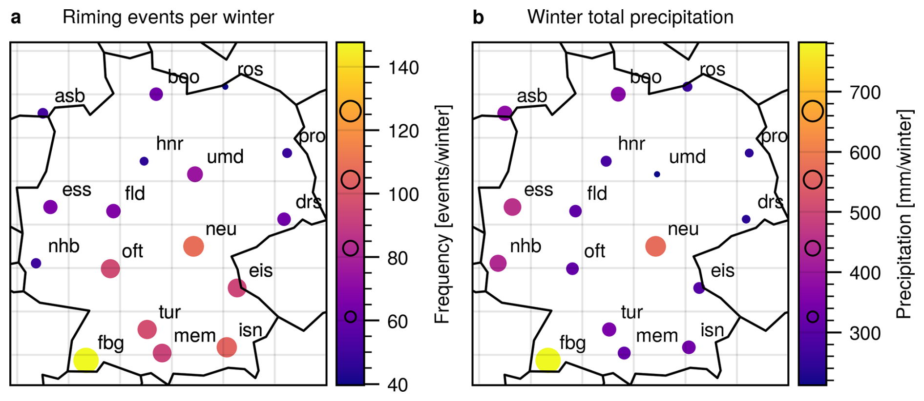
Figure 10 Spatial distribution of riming event frequency (a) and total wintertime precipitation (b) in Germany.

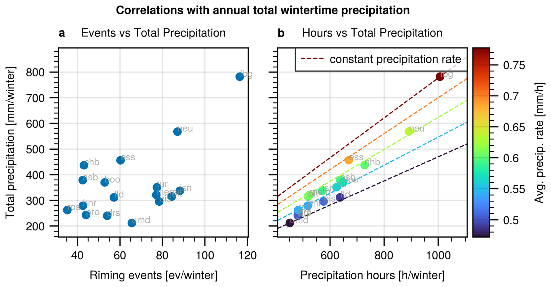
Figure 11 (a) Correlation between the number of riming events and total wintertime precipitation. (b) Correlation between the number of precipitation hours and total wintertime precipitation. Their ratio form the average precipitation rate and is shown by the colors.

3.3 Spatial Distribution and Relation to Surface Precipitation

With the possibility to retrieve riming from operational radars, we are able to analyze the spatial distribution of riming probability over larger areas for the first time. Figure 10a shows the number of riming events per winter (November–April) for the different operational radar sites in Germany. The values are corrected for differences in the radar uptime. Generally, we see less riming events for the northern radars compared to the ones in southern Germany. By far the most events are detected for the Feldberg (fbg) radar, located on top of the Feldberg mountain at 1494 m elevation above sealevel in southwestern Germany. Also the Neuhaus radar at 880 m elevation shows enhanced riming. In order to investigate this pattern, it is instructive to look at the precipitation distribution in Germany. For this task, we analyze the quality controlled hourly precipitation product provided by the German Meteorological Service (DWD, 2025). The measurements are performed by PLUVIO or raineH3 tipping buckets (Saha et al., 2021; Quinlan, 2022). For every operational radar site, we average the winter precipitation accumulation from the nearest surface weather station for the years 2005 to 2025 in order to estimate the local mean wintertime precipitation. There is always a station in less than 18 km radius. For the Feldberg site, there is a surface weather station directly next to the radar at the mountain top. Figure 10b depicts the resulting mean wintertime precipitation. We can see the typical German pattern with a wet South and a dry Northeast (Kreienkamp, 2022). The Feldberg radar shows strong precipitation enhancement with 782 mm per winter, more than twice the average of 336 mm per winter for all other stations. The correlation between riming and total wintertime precipitation can be seen in Fig. 11a. There is a positive correlation between the number of riming events and precipitation amount. Obviously, it is not surprising to detect more riming events at sites which are more often affected by precipitating systems. In the following, we want to investigate whether sites with greater riming and total precipitation also experience more intense precipitation, or if the increased totals are just due to longer precipitation duration. For this task, we decompose the total precipitation per site, T, into the product of the number of hours with precipitation, N, and the average hourly precipitation rate $\widehat{R}$:

$$\begin{array}{}\text{(8)}& {\displaystyle }T=N\times \widehat{R}\text{(9)}& {\displaystyle }\widehat{R}={\displaystyle \frac{\mathrm{1}}{N}}\sum _i^N{R}_i\end{array}$$

here, R_i are the hourly precipitation rates and N is the number of hours with at least 0.1 mm h⁻¹ precipitation. N and $\widehat{R}$ are not fully independent. Sites with more precipitation hours also tend to have stronger precipitation rates, as can be seen from Fig. 11b. Figure 12 shows the relation to the riming events. From Fig. 12a, we see that the high number of events at Neuhaus and Feldberg can mostly be explained by the greater number of precipitation hours. The number of events per hour at those two sites lies near the median of the distribution observed across all other sites. Neglecting the outliers Neuhaus and Feldberg, there is almost no correlation between number of precipitation hours and riming events for the remaining sites (grey box in Fig. 12a with a pearson correlation coefficient −0.06). In Fig. 12b, we see the correlation between riming events and average precipitation rate, with a focus on stronger precipitation events of at least 1 mm h⁻¹. The correlation coefficient is 0.36 (grey box in Fig. 12b, omitting the Feldberg radar).

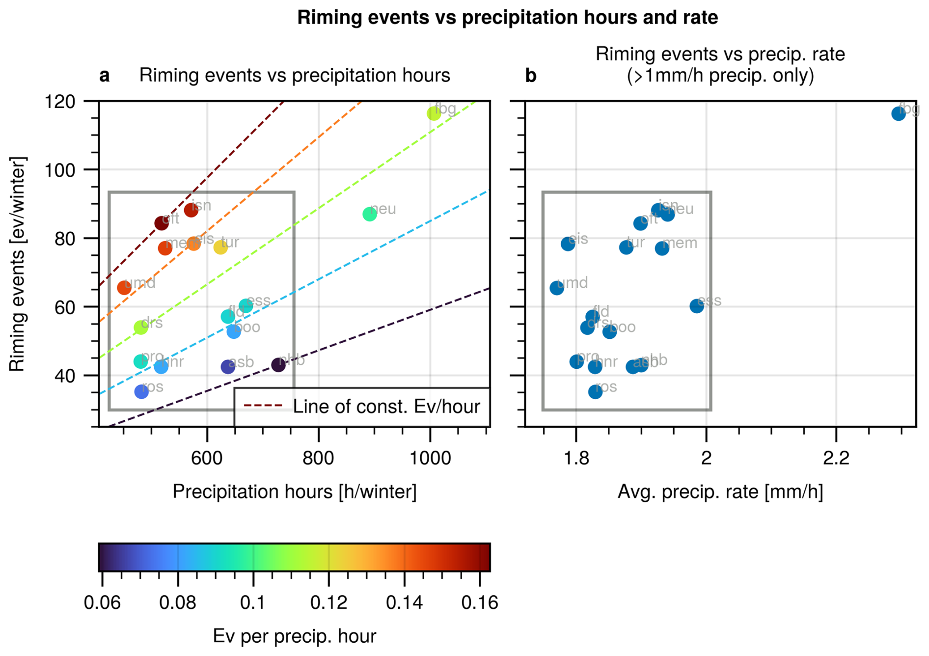
Figure 12 (a) Correlation between the number of riming events and precipitation hours per winter. Their ratio is shown by the colors. Pearson correlation within the grey box: −0.06. (b) Correlation between the number of riming events and average precipitation rate per winter. Pearson correlation within the grey box: 0.36.

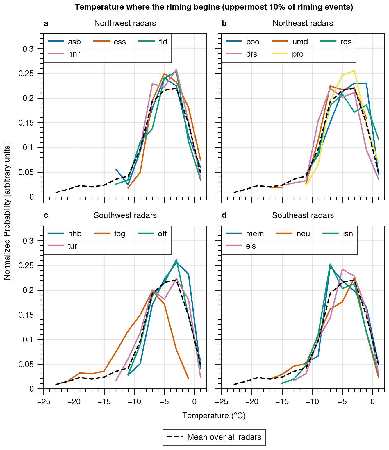
Figure 13 Temperature distribution of the riming event top (highest level with significant riming per event). For better visibility, the sites are separated into four subregions. The histograms are corrected for differences in radar uptime, elevation and riming frequency, as described in Sect. 2.9.

3.4 Riming Onset Temperature Distribution

We define the onset temperature of a riming event as the temperature at the highest level with significant riming detections. That means, for each event, we take the temperature of the uppermost 10 % of range gates, in order to get a robust estimate of the temperature level where we see the first indications of riming. The temperatures are based on radiosonde profiles. In Fig. 13, we see the onset temperature frequency distribution. The histograms are corrected for differences in radar uptime, elevation and riming frequency, as described in Sect. 2.9. Despite the variability in the absolute frequency of riming events, which we already analyzed in Sect. 3.3, the relative temperature distribution is very consistent between the different sites. In all cases, we see that strong riming occurs almost exclusively at temperatures warmer than −15 °C. This strengthens the results of Kneifel and Moisseev (2020) and Ockenfuß et al. (2025), who found similar patterns based on the analysis of four, respectively two European cloud radar sites. The notable exception here is the Feldberg radar, which has a distribution shifted significantly towards colder temperatures (see Appendix C for a statistical analysis). Here, we have to keep in mind that data at temperatures warmer than −5 °C is scarce at the Feldberg radar in winter. The slightly enhanced values at temperatures colder than −10 °C, compared to the other sites, may be attributed to differences in updraft speed, as further discussed in Sect. 4.

4 Discussion

This study allows us for the first time to investigate the occurrence of strong riming over a multi-year period and across a larger region, covering multiple sites throughout Germany. This provides us with the opportunity to assess systematic relationships between riming aloft and surface precipitation characteristics that could not be addressed in earlier, more limited studies.

Intuitively, one might expect that sites experiencing a larger number of precipitation hours at the surface would also exhibit a higher number of riming events aloft. However, our results do not support this assumption. While some sites record around 700 precipitation hours per winter but only about 40 riming events, other sites show roughly 500 precipitation hours yet up to 90 riming events (Fig. 12a). As a consequence, the relative frequency of riming varies substantially between sites, and no correlation between precipitation duration and riming occurrence can be identified.

In contrast, when precipitation intensity is considered instead of precipitation hours, a different picture emerges. We observe a moderate positive correlation between the average surface precipitation intensity and the frequency of riming events (Fig. 12b). This finding is in line with previous studies that have suggested a link between stronger precipitation rates at the surface and riming aloft. For example, surface observations have shown that rime mass can constitute the majority of total surface precipitation mass (e.g. Harimaya and Sato, 1989; Zhang et al., 2021). Based on a one-month measurement campaign in the Alps, Grazioli et al. (2015) reported a correlation between snow accumulation and the fraction of rimed precipitation. Similarly, Moisseev et al. (2017) observed a tendency toward stronger precipitation rates during riming events in a field campaign in Finland, although they noted that the effect might not be statistically significant. More recently, Ockenfuß et al. (2025) conducted a long-term analysis at a single German research site (Jülich) using 13 years of disdrometer-derived rain rates and found a statistically significant difference between rimed and unrimed precipitation, with rain rates exceeding $\mathrm{1}\mathrm{mm},{\mathrm{h}}^{-\mathrm{1}}$ occurring more frequently during riming aloft.

From a purely microphysical perspective, a correlation between riming and precipitation rate appears plausible. In mixed-phase clouds where supercooled liquid water and ice coexist, riming provides an efficient pathway for the rapid conversion of liquid water into ice. The resulting increase in particle density leads to higher sedimentation velocities of rimed ice particles and thus to an enhanced mass flux within the cloud. At the same time, cloud microphysical processes are closely linked to cloud dynamics. Supersaturation conditions that allow the formation and maintenance of supercooled liquid water are often associated with stronger upward motions. Enhanced lifting generally leads to increased condensation and deposition rates and therefore to higher precipitation intensities, even in the absence of riming. In this sense, riming may frequently occur as a consequence of the dynamical conditions associated with stronger lifting. Nevertheless, for clouds with comparable thermodynamic and dynamical conditions, the occurrence of riming is still expected to further increase precipitation intensity.

This interpretation is consistent with our finding of more frequent riming at higher-elevation sites such as Feldberg and Neuhaus, where orographic forcing is likely to enhance upward motions. Conversely, the generally lower number of riming observations in the Northern German Lowlands (Fig. 10a) supports the notion that weaker lifting conditions reduce the occurrence of riming in these regions.

Another robust feature in riming observations is the typical temperature range they occur. Consistent with earlier studies (e.g. Kneifel and Moisseev, 2020; Ockenfuß et al., 2025), riming is almost exclusively observed at temperatures between 0 and −15 °C. In our data set, this temperature dependence is remarkably consistent across nearly all sites (Fig. 13). The only notable deviation from this pattern is found at the Feldberg site, where the temperature distribution of riming events is significantly shifted toward colder values. A plausible explanation for this shift is the strong influence of orography at Feldberg, which likely modifies the dynamical environment in which riming occurs. In particular, updraft speed may play a key role in shaping the temperature distribution of riming events.

Both modeling studies (e.g. Pinsky and Khain, 2002) and observational evidence (e.g. Snider and Brenguier, 2000) indicate that stronger updrafts promote the activation of a larger number of cloud condensation nuclei due to enhanced supersaturation. As a consequence, more numerous but smaller supercooled liquid droplets form at a given altitude compared to weaker updraft conditions. These droplets also experience faster upward transport, which further limits their growth by condensation. Because riming efficiency depends strongly on droplet size (DeLaFrance et al., 2024) and decreases sharply for droplets smaller than about 20 µm (e.g. Lasher-Trapp, 2022), riming becomes inefficient at warmer levels in such environments. The altitude, and thus the temperature, at which droplets have grown sufficiently large for efficient riming is therefore shifted upward, reducing the warm side of the riming temperature histogram.

In addition, stronger updrafts increase the residence time of snowflakes at higher altitudes, where they can continue to grow by vapor deposition. This prolonged growth phase may enhance riming signatures at lower temperatures and thus amplify the cold side of the temperature distribution. Taken together, these mechanisms provide a physically consistent explanation for the cold shift observed in the riming temperature distribution at the Feldberg site.

4.1 Methodological Limitations and Sources of Uncertainty

At this point, potential methodological limitations related to radar sensitivity need to be addressed. In particular, the height- and site-dependent clutter filter described in Sect. 2.4 introduces variations in effective radar sensitivity between the sites (Fig. A1 shows the corresponding clutter threshold curves for all 17 radars). In the height range between 0 and 5 km, which is most relevant for riming detection, the mean sensitivity across all sites is −14.2 dBZ, with a standard deviation of 2.2 dBZ. To assess whether these differences could influence the observed variability in riming frequency, we correlated the site-specific radar sensitivity with the number of detected riming events. This analysis revealed no relationship between the two (Pearson correlation coefficient of 0.05), indicating that the observed differences in riming frequency are unlikely to be driven by variations in radar sensitivity.

Another factor that requires careful consideration is the influence of strong vertical air motions on the riming detection. Our analysis is restricted to midlatitude, stratiform wintertime clouds. In these clouds, the large scale lifting velocities are usually in the order of tenths of cm s⁻¹ and therefore much less than the rimed particle velocities of at least 1.5 m s⁻¹ (e.g. Shupe et al., 2008; Roh et al., 2025). However, orographically induced gravity waves may still occur, particularly in mountainous regions. Since our method relies on vertical Doppler velocity measurements, there is a potential risk that wave-induced vertical motions could be misinterpreted as riming signatures.

In our opinion, there are several reasons why such a bias in our results is unlikely. First, we apply a dedicated filter designed to identify and remove regions dominated by oscillatory vertical motions. Because the performance of this filter could, in principle, depend on temporal resolution, we validated it using high-temporal-resolution measurements, as described in Sect. 2.6. Second, the overall topography in Germany is still relatively moderate compared to more complex mountain environments such as the Alps. The Feldberg radar, located at 1494 m above sea level, represents the highest site in the network, while all other radars are situated below 1000 m. In addition, when radars are deployed in mountainous terrain, they are often installed at the highest point in their immediate surroundings. Combined with the blind range of approximately 600 m inherent to our setup, this implies that the observations generally sample the atmosphere above the most strongly terrain-influenced layers. This reduces, for example, the risk of persistent lee-side subsidence being misinterpreted as riming signals, as it would be the case if the radar is located at the mountain base.

Further support for a primarily microphysical interpretation of the results is provided by the temperature distributions associated with riming events. As shown in Sect. 3.4, these distributions are remarkably consistent across nearly all sites. If orographic gravity waves were a dominant source of false riming detections, one would expect signatures at a wider range of altitudes and temperatures, rather than a well-defined and consistent temperature dependence. The only notable deviation from this pattern is the cold shift observed at the Feldberg site. As discussed above, both theoretical considerations and observational evidence offer microphysical explanations for this cold shift. Nevertheless, a dynamical contribution at this particular location cannot be excluded. Compared to the Neuhaus radar, which is also situated in a low-elevation mountain range (Thuringian Forest), the orography surrounding the Feldberg radar is more complex, and the radar is located closer to the initial rise of the Black Forest mountain range. Together with the higher elevation of the site and the orientation of the Black Forest being largely orthogonal to the prevailing westerly flow, orographically induced dynamical effects remain an alternative explanation for the observed cold shift and can in principle not be ruled out conclusively.

5 Conclusions

In this study, we successfully adapted a riming detection algorithm – originally developed for vertically pointing cloud radars – to the vertically looking “birdbath” scan of the operational German C-band weather radar network. The riming detection is based on the typical fallspeed of more than 1.5 m s⁻¹ of strongly rimed particles (Kneifel and Moisseev, 2020). This transfer illustrates the considerable potential of operational birdbath scans, not only for routine monitoring but also for quantitative analysis and cloud microphysical research. Included in the method is a fast and fully automatic filtering method to remove clutter from the raw radar data. Furthermore, our riming retrieval includes an operational melting layer detection algorithm, which could serve as a valuable standalone product – offering support to forecasters or providing input for more advanced retrieval schemes.

During the adaptation process, we discovered several general challenges that arise when applying algorithms designed for research cloud radars to operational systems. In particular, differences in radar frequency bands, coarser time resolution, and the absence of auxiliary measurements or model profiles must be addressed. While we initially expected the temporal resolution of 5 min to be a major limitation, we found that the primary challenges stem from the lack of auxiliary sensor and model data, which is nowadays often used in radar based retrievals.

Our analysis of the results reveal a remarkably consistent temperature dependence of riming events across all sites, reinforcing results from previous studies that strong riming is confined to temperatures warmer than −15 °C. Moreover, we find a climatological link between the frequency of riming and both the total amount and intensity of precipitation, supporting a physically plausible connection between riming and enhanced precipitation rates.

Through the riming case study, we demonstrate the general scientific value of utilizing operational radar networks for atmospheric research. These systems offer equidistant spatial coverage with consistent quality monitoring and generate vast amounts of data within relatively short time periods. This enables the creation of robust long-term statistics and climatologies, and facilitates comparisons across different microclimatic regions over a larger area. In light of these results, we believe the full potential of operational birdbath scan data remains still underutilized. For example, the European radar network OPERA consists of over 200 radars, with the majority performing routine birdbath scans. Integrating these observations into established research frameworks such as Cloudnet would increase their visibility and scientific impact, providing a complement to the few but sensor-rich Cloudnet research stations. As is common in Cloudnet for the research stations, the archiving of vertical profiles from common numerical weather models (like temperature, pressure, wind, and more) for the operational radar sites will provide a valuable opportunity for longterm comparisons. To further enhance the utility of operational radar sites, we advocate for the installation of basic surface meteorological sensors – like temperature, pressure, and wind measurements – at all sites. In addition, the installation of a low-cost micro rain radar (Peters et al., 2002) can fill the lowermost 600 m to enable the creation of continuous profiles through the full troposphere. The live provision of such profiles to operational weather forecasters could be useful for nowcasting applications.

Finally, expanding this approach beyond Germany could yield significant benefits. Systematically recording birdbath scans from operational radar networks across Europe and providing them in a standardized format on a shared platform like Cloudnet would create a unique dataset. Such an initiative would be a major step forward for large-scale, data-driven cloud and precipitation research across the continent.

Appendix A: Reflectivity Histograms and Thresholds for all Radar Sites

Figure A1 shows the vertically resolved reflectivity histograms and the derived signal-clutter threshold for all 17 radar sites.

Figure A1 Same as Fig. 2c, but for all of the 17 radar sites in Germany. The blind range is shown as grey shading.

Appendix B: Sobel Filter Gradient

Figure B1 shows the velocity gradient resulting from the application of a normalized 3×3 Sobel filter to the Doppler velocity of the C-band birdbath scan.

Figure B1 Gradient resulting from the application of a normalized 3×3 Sobel filter to the Doppler velocity of the C-band birdbath scan.

Appendix C: Statistical Analysis of Temperature Differences

In order to asses whether the distributions in riming event top temperature are significantly different between two radar sites, we model each observation at a specific site and temperature as a bernoulli experiment. We select two sites and denote with variable s the first site with value s=0 and for the second site s=1. Figure 6 can be interpreted as the number of trials per site and temperature. This way, differences in radar uptime and altitude are accounted for in the model. Figure C1 shows the number of hits, i.e. riming detections, per site and temperature. We model the riming probability as a function of temperature with a gaussian function, as shown in Eq. (C1)

$$\begin{array}{}\text{(C1)}& p\left(T\right)=e^{c_{\mathrm{0}}-c_{\mathrm{1}}s}{e}^{-\frac{(T-(c_{\mathrm{2}}+c_{\mathrm{3}}s){)}^{\mathrm{2}}}{\mathit{\alpha }}}\end{array}$$

Since, as discussed in Sect. 2.9, there are differences in the total riming frequency between the sites, we include a site dependent prefactor. Shifts in temperature are expressed by a site dependent mean of the Gaussian. We assume equal width for both sites. In logspace, Eq. (C1) transforms into a (generalized) linear model with three statistical variables s, T and T².

$$\begin{array}{}\text{(C2)}& \ln \left(p\right)={\mathit{\beta }}_{\mathrm{0}}+{\mathit{\beta }}_{\mathrm{1}}s+{\mathit{\beta }}_{\mathrm{2}}T+{\mathit{\beta }}_{\mathrm{3}}Ts+{\mathit{\beta }}_{\mathrm{4}}{T}^{\mathrm{2}}\end{array}$$

We used the fact that s²=s. The coefficients read:

$$\begin{array}{}\text{(C3)}& \begin{array}{rl}{\mathit{\beta }}_{\mathrm{0}}=& c_{\mathrm{0}}-{\displaystyle \frac{c_{\mathrm{2}}^{\mathrm{2}}}{\mathit{\alpha }}},{\mathit{\beta }}_{\mathrm{1}}=-{\displaystyle \frac{\mathrm{2}{c}_{\mathrm{2}}{c}_{\mathrm{3}}-c_{\mathrm{3}}^{\mathrm{2}}}{\mathit{\alpha }}}-c_{\mathrm{1}},\\ & {\mathit{\beta }}_{\mathrm{2}}={\displaystyle \frac{\mathrm{2}{c}_{\mathrm{2}}}{\mathit{\alpha }}},{\mathit{\beta }}_{\mathrm{3}}={\displaystyle \frac{\mathrm{2}{c}_{\mathrm{3}}}{\mathit{\alpha }}},{\mathit{\beta }}_{\mathrm{4}}=-{\displaystyle \frac{\mathrm{1}}{\mathit{\alpha }}}\end{array}\end{array}$$

Our null hypothesis is that both sites follow the same temperature distribution, i.e. c₃=0. In this case, the coefficient β₃ vanishes. Therefore, if β₃ significantly improves the fit, the sites can be assumed to have significantly different temperature dependence. Figure C2 shows c₃, the difference in the mean temperature, for all radar combinations, where β₃ is significant (significance level p<0.01). As we can see, the Feldberg radar is the only one, which shows a significant shift in mean temperature with respect to all other radars. Moreover, the difference in the average difference in the temperature mean c₃ is much larger than for all other radar combinations.

Figure C1 Same as Fig. 13, but not corrected for any of the effects discussed in Sect. 2.9.

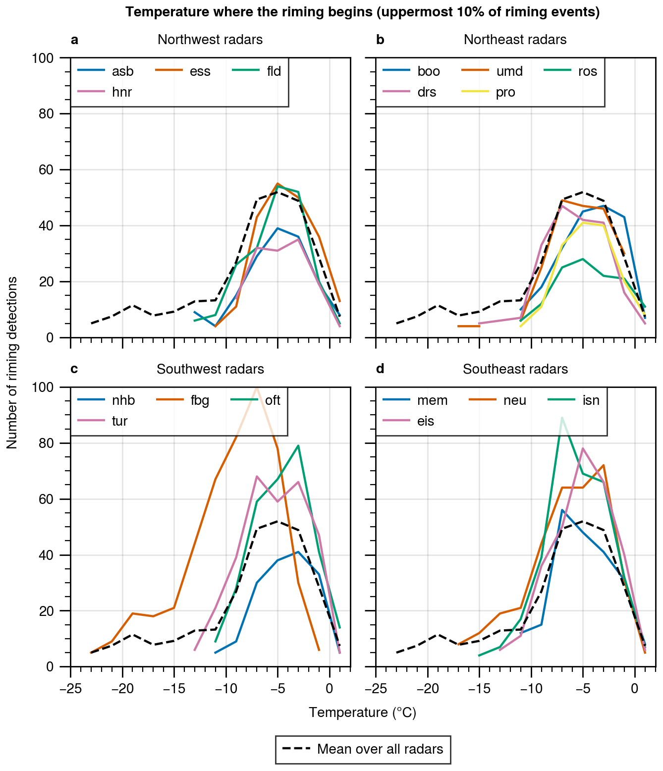
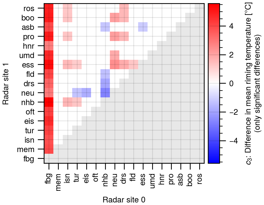
Figure C2 Difference in the average riming onset temperature. Shown are only significant differences with a significance level of better than 0.01. Red colors mean that radar 1 has a higher mean than radar 0.