A novel framework for automatic scanning radar pointing calibration using the Sun

A high accuracy of antenna beam pointing is essential for weather and cloud radars in order to precisely locate clouds and precipitation. It is also a critical requirement for estimating the horizontal wind field or retrieving particles' vertical motions.

We present a general framework for radar pointing calibration using the Sun as a reference target. The workflow is structured into three steps: (i) measurement and analysis of individual Sun scans, (ii) estimation of scanner inaccuracies from a series of scans, and (iii) correction of these inaccuracies. Our approach is radar-agnostic and applicable to any instrument equipped with a two-axis pan-tilt scanner and a parabolic antenna. General recommendations for Sun scan implementation are given, and the full calibration process is demonstrated using a Mira-35 cloud radar. The method allows retrieval of a comprehensive set of parameters, including beamwidth in two orthogonal directions, pedestal tilt, axis misalignments, encoder offsets, gear backlash, and the receiver-scanner time offset. With this approach, absolute pointing accuracy better than 0.1° can be achieved, and relative changes as small as 0.01° can be detected. To facilitate automatic application, we provide the open-source Python library SunscanPy for radar pointing calibration. This toolset is especially valuable for stationary radars and radar networks, where it enables automatic monitoring of long-term pointing stability. Finally, we introduce a novel automatic pointing correction scheme based on inverse kinematics. Once the scanner inaccuracies are estimated, the required motor positions can be computed to compensate for the inaccuracies, without mechanical adjustments. Such functionality is particularly advantageous for mobile radars, research campaigns, or remote deployments, where frequent mechanical leveling is necessary but often difficult to perform.

1 Introduction

Accurate antenna pointing is crucial for a wide range of radar applications. Applications that rely on precise georeferencing, such as scanning weather radars, are particularly sensitive, since even small pointing errors lead to spatial displacements of observed features. For example, a 1° change in pointing direction leads to 3.5 km displacement at a distance of 200 km. For vertically pointing radars, pointing accuracy is equally critical for the correct measurement of vertical velocities. Since vertical air motion and particle sedimentation speeds are typically an order of magnitude smaller than horizontal wind, even small pointing errors can lead to large biases. A simple calculation illustrates this: assuming a horizontal wind speed of 30 m s⁻¹, as is common in the higher atmosphere (Holton and Hakim, 2013), a mispointing of 0.2° produces an apparent vertical velocity of ±10.5 cm s⁻¹, depending on the wind direction. This is a non-negligible error, given the typical sedimentation velocity of ice around 30 to 50 cm s⁻¹ (Houze, 2014). In principle, modern Doppler radars are capable of measuring velocities with a precision of less than 5 cm s⁻¹ (METEK GmbH, 2013). Furthermore, precise pointing is also indispensable in advanced applications such as multi-frequency measurements, where two radars must probe the same volume simultaneously, which demands near-perfect beam alignment (Kneifel et al., 2016; Tridon and Battaglia, 2015).

To ensure accurate pointing, a variety of calibration methods have been developed. One straightforward approach is the use of hard targets at a known position or ground-clutter (e.g. Altube et al., 2016). While effective in principle, hard targets are not always available, probe only one specific scanner configuration, and ground-clutter-based methods may be compromised by precipitation or anomalous atmospheric propagation conditions (Altube et al., 2016). A widely adopted alternative is to use the Sun, which acts as a natural microwave source. The advantage of Sun-based calibration is that it requires minimal additional effort: operational radar measurements occasionally intersect the solar disk by chance, and these data can be used even without specific campaigns. For scanning research weather radars, dedicated solar scans are often performed as part of calibration routines. The benefits of solar calibration are now widely acknowledged (e.g. Holleman et al., 2022), and some radar manufacturers have integrated corresponding procedures into their operational software (e.g. Radiometer Physics GmbH (RPG), 2024).

A number of studies have investigated the use of the Sun for radar calibration, with different emphases on pointing accuracy and antenna characterization. Early work by Baars (1973) discussed cosmic sources such as the Sun for large antenna calibration. In addition to antenna pointing, other antenna parameters, such as aperture or antenna beam pattern, were derived from measurements on radio sources. Later, Mano and Altshuler (1981) discussed the Sun as a potential calibration target with a well-known position, focusing primarily on elevation biases. In a review of radar calibration methods, also Manz et al. (2000) highlight the Sun as an excellent source to calibrate position accuracy. Arnott et al. (2003) demonstrated that solar observations could also be used to estimate the azimuth orientation of a mobile radar system mounted on a truck. Similarly, Darlington et al. (2003) explored the potential of solar signals for calibrating operational weather radars in the United Kingdom. Their study emphasized the advantage of performing the calibration without disturbing the ongoing operational scan strategy. Due to the limited maximum elevation angle of their radar (4°), their analysis was restricted to azimuth biases. Further developments were made by Huuskonen and Holleman (2007) and later by Holleman et al. (2010), who refined the methodology for operational weather radars. In particular, they introduced corrections for atmospheric refraction, which is especially relevant for low-elevation measurements where the apparent solar position is significantly displaced. Muth et al. (2012) proposed a technique based on the analogy between radar and theodolite systems, using solar observations to quantify and correct pointing errors in both azimuth and elevation. Their evaluation of a single Sun scan is based on Huuskonen and Holleman (2007). More recently, Altube et al. (2015) demonstrated how the Sun can be used for online monitoring of the antenna alignment of an operationally scanning weather radar. In a subsequent study, Altube et al. (2016) then compared ground-clutter-based and Sun-based antenna pointing calibration methods and found the methods based on the Sun to be generally superior. Recently, Frech et al. (2019) assessed the antenna pointing accuracy in both azimuth and elevation for a polarimetric research radar based on dedicated solar box scans. In addition to pointing, the Sun has also been used to characterize the antenna beam pattern. Reimann and Hagen (2016) employed solar scans to measure the antenna beam shape and demonstrated good agreement with the expected response to a point source. While our work focuses on antenna pointing calibration, the beam pattern retrieval comes as a natural by-product of the same procedure.

Although these studies have shown in the past that the Sun provides an excellent target for antenna pointing calibration, two important deficiencies remain. First, there is no general, radar-agnostic framework to calibrate the pointing from Sun scans. While manufacturers provide proprietary tools, these are often tailored to specific radar systems and are not easily transferable. Yet, the underlying geometry is universal: virtually all weather and cloud radars operate on a two-axis pan-tilt mechanism, and once the solar data are recorded, the processing steps are conceptually identical across platforms. Second, existing calibration workflows typically assume that mechanical correction of the scanner is required once biases are identified. We argue that an alternative is possible: active, software-based correction of mispointing. By interpreting the radar scanner as a simple kinematic chain with two rotational joints, the problem is directly analogous to inverse kinematics in robotics. Inverse kinematics is the process of determining the joint positions of a kinematic chain, which correspond to a desired location and orientation of the chain end. Using inverse kinematics, the radar controller software can compensate for misalignments, instead of requiring mechanical adjustment of the system.

The objective of this publication is therefore twofold. First, we present a novel, generic framework for scanning radar pointing calibration, subdividing the process into three well-defined, consecutive steps. By combining multiple Sun scans, our method is able to derive the full set of scanner offsets and inaccuracies in both axes, including velocity-dependent dynamic biases. To make this methodology accessible to the broader community, we provide SunscanPy (Ockenfuß and Köcher, 2026a), a general and open-source Python package for radar antenna pointing calibration using solar observations. The software is designed to be radar-independent and provides a standardized way to derive scanner inaccuracies. Second, we demonstrate a method for software-based pointing correction, in which identified biases are incorporated into the radar controller, thereby avoiding the need for mechanical realignment.

The remainder of this publication is organized as follows. Section 2 describes the theoretical background of antenna pointing calibration using the Sun and introduces a mathematical nomenclature. Section 3 demonstrates the process using measurements of a cloud radar. Both sections contain three dedicated subsections, reflecting the three steps of the calibration method. The achievable pointing accuracy of the method is discussed in Sect. 4.2. Section 5 introduces the SunscanPy Python implementation. Section 6 summarizes the results and provides perspectives on possible areas of application.

2 Methods

The whole process of scanner calibration with the Sun can be divided into three distinct steps, as illustrated in Fig. 1. In step 1, we use the Sun as a source of microwave emission in the sky with a precisely defined trajectory. Probing this source with the radar antenna, we can record the position of the scanner axis encoders when looking at a defined position relative to the Sun, e.g. the center of the solar disk. Repeating step 1 over the course of multiple days and times, we obtain a collection of scanner positions with the corresponding beam locations in the sky. In step 2, we use this dataset to estimate unknown parameters that define the scanner system. In step 3, we apply the knowledge of these parameters when pointing to a target. We can either correct the scanner mechanically like illustrated in step 3a, or do a software-based correction like depicted by step 3b.

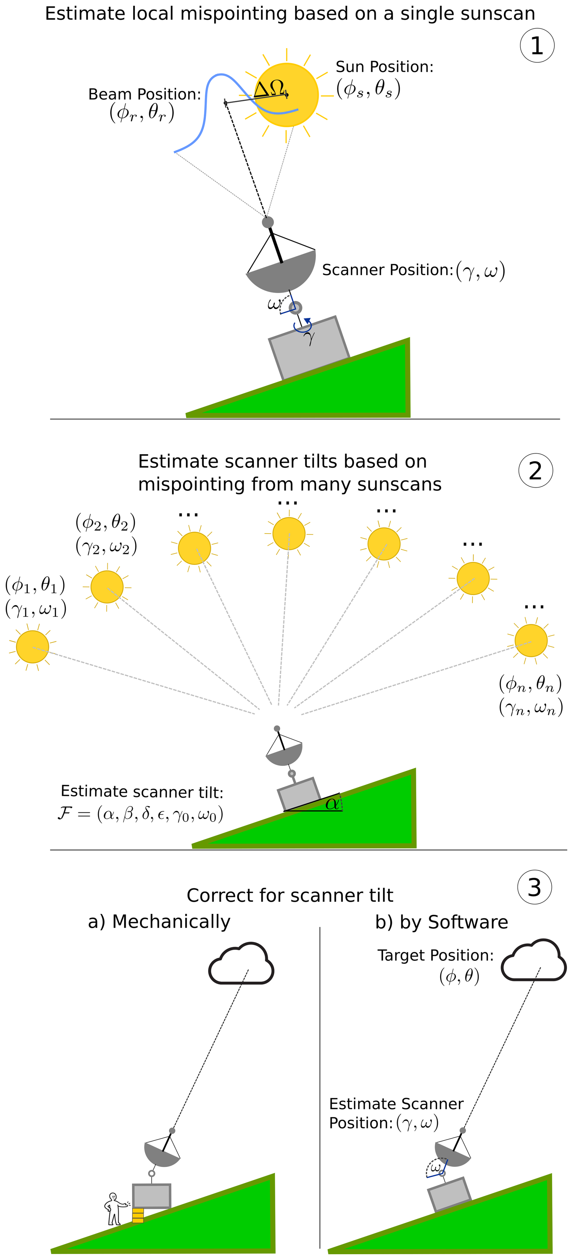
Figure 1 Schematic illustration of the full pointing calibration procedure. Step 1: estimation of local mispointing from a single Sun scan. Step 2: estimation of scanner inaccuracies based on multiple Sun scans. Step 3: correction of scanner inaccuracies.

2.1 Scanner Inaccuracies

Pointing directions in the sky can be described by two spherical coordinates, where $\mathit{\varphi }\in \left[\mathrm{0}\mathit{°},\mathrm{360}\mathit{°}\right]$ denotes the azimuth angle and $\mathit{\theta }\in \left[\mathrm{0}\mathit{°},\mathrm{90}\mathit{°}\right]$ is the elevation angle. We follow the common convention in radar science that 0° elevation corresponds to pointing horizontally. Scanning radars usually have a two-axis scanner mechanism, where one axis corresponds to the movement in azimuth direction and another axis on top of the first moves in elevation direction. We denote the position of those axes by γ and ω, respectively. Usually, it is assumed that a movement in γ directly corresponds to a movement in ϕ and similarly for ω and θ. However, this is only the case for a perfect scanning mechanism. In reality, axis positions are not perfectly equal to pointing directions, due to multiple system imperfections: axis encoders can have offsets, the axes are not perfectly orthogonal, or the whole system is tilted with respect to the celestial hemisphere. Therefore, a strict separation between axis positions (γ,ω) and celestial pointing (ϕ,θ) is necessary. We describe the mapping between axis positions and celestial pointing of the radar by a forward model M_𝒫:

$$\begin{array}{}\text{(1)}& M_{\mathcal{P}}:(\mathit{\gamma },\mathit{\omega })\mapsto (\mathit{\varphi },\mathit{\theta }).\end{array}$$

Finding M_𝒫 is the main goal of the methods described here. M_𝒫 depends on multiple parameters 𝒫, which describe the imperfections of the scanner alignment and mechanics. There are seven static parameters:

$$\begin{array}{}\text{(2)}& \mathcal{P}=\left(\mathit{\alpha },\mathit{\beta },\mathit{\delta },\mathit{ϵ},{\mathit{\gamma }}_{\mathrm{0}},{\mathit{\omega }}_{\mathrm{0}},\mathit{\chi }\right).\end{array}$$

The individual static scanner parameters are illustrated in Fig. 2 and defined as follows:

• α: pedestal tilt towards West or East

• δ: pedestal tilt towards North or South

• ϵ: ideally the radar beam should be perpendicular to the axis of the elevation rotation of the scanner. ϵ describes the offset from this goal.

• β: gimbal tilt. Ideally the axis of the elevation and axis of the azimuth rotations of the scanner should be perpendicular. β describes the offset from this goal. The gimbal tilt β and the antenna tilt ϵ have the same effect if the scanner is pointed vertically or close to vertically. If the beam is pointing at the horizon or close to the horizon then the antenna tilt ϵ causes an azimuth offset but the effect of the gimbal tilt β vanishes.

• γ₀: offset between actual azimuth axis position and the value returned by the scanner motor encoder. This value is sometimes known as the “northangle”.

• ω₀: offset between actual elevation axis position and the value returned by the scanner motor encoder.

• χ: if not pointing vertically, the weight of the antenna can cause elastic deformations, which cause the scanner structure to bend. This causes an elevation offset, which depends on the current elevation position. We model this effect as an elevation position offset of the form ω_flex = χcos (ω). χ is usually negative.

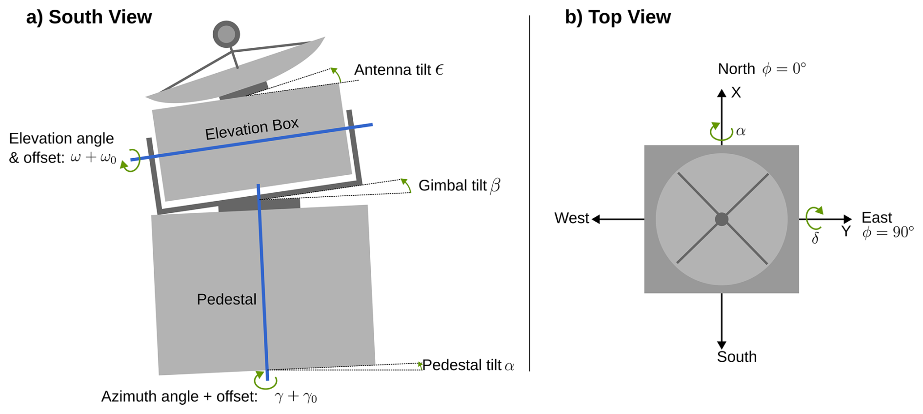
Figure 2 Inaccuracies of the scanner leading to beam pointing offsets, with the axes positioned at γ = 0° and ω = 90°. (a) View from the South. (b) View from the top. The sign convention of each parameter is indicated by green arrows, which point into the positive direction of movement. Positive α tilts the radar West, positive δ tilts the radar North. Positive γ tilts the dish clockwise, if viewed from the top. For γ = 0° and ω = 0°, the dish points to the North. For γ = 0°, positive ω tilts the elevation box clockwise, if viewed from the West.

We denote a perfectly accurate scanner as M_ℐ, with $\mathcal{I}=(\mathrm{0},\mathrm{0},\mathrm{0},\mathrm{0},\mathrm{0},\mathrm{0},\mathrm{0})$. For such a perfect scanner, axis positions and celestial pointing are identical (at least, as long as ω ≤ 90°): γ=ϕ and ω=θ.

In addition to the static scanner parameters, there are also dynamic parameters. Dynamic means that their effect on the beam pointing depends on the velocity of the axes $(\dot{\mathit{\gamma }},\dot{\mathit{\omega }})$. We consider the following dynamic parameters:

• b_γ: backlash in the azimuth axis. For example, this can be caused by play in the gears of the azimuth axis. As a consequence, this creates a hysteresis in the system, where the beam is always lagging behind the position indicated by the scanner motors. The backlash only depends on the direction of movement. The effect of the backlash on the actual position $\stackrel{\mathrm{̃}}{\mathit{\gamma }}$ of the azimuth axis can be modeled as $\stackrel{\mathrm{̃}}{\mathit{\gamma }}=\mathit{\gamma }+b_{\mathit{\gamma }}\text{sign}\left(\dot{\mathit{\gamma }}\right)$

• t₀: time offset between the time of recording of the motor positions and the time of recording of the signal. It causes a lag between motor positions and beam, but in contrast to the lag caused by the backlash, the lag due to the time offset depends on the speed of motion. In the absence of acceleration of the motors, the actual positions can be calculated as $\stackrel{\mathrm{̃}}{\mathit{\gamma }}=\mathit{\gamma }+t_{\mathrm{0}}\dot{\mathit{\gamma }}$ and $\stackrel{\mathrm{̃}}{\mathit{\omega }}=\mathit{\omega }+t_{\mathrm{0}}\dot{\mathit{\omega }}$.

We assume that the effect of the dynamic parameters is the same, regardless of the scanner pointing position in the sky. Therefore, they can simply be modeled as offsets to the scanner coordinates:

$$\begin{array}{}\text{(3)}& M_{\mathcal{P}}\left(\mathit{\gamma }+b_{\mathit{\gamma }}\text{sign}\left(\dot{\mathit{\gamma }}\right)+t_{\mathrm{0}}\dot{\mathit{\gamma }},\mathit{\omega }+t_{\mathrm{0}}\dot{\mathit{\omega }}\right).\end{array}$$

2.2 Step 1: Estimate Local Mispointing

If the Sun were a perfect point source and the radar emitted an infinitely narrow beam, step 1 would not be necessary to get a pair of referenced scanner coordinates. In that idealized case, we could simply scan across the sky until the beam intersects the point-like Sun, record the corresponding scanner coordinates, and directly assign them to the absolute solar position.

In reality, the Sun appears as an extended, moving disk and the radar beam exhibits a finite width. Consequently, the measured signal represents a broadened response, and we must determine the apparent center of the Sun within the data. Similar to Huuskonen and Holleman (2007), we will do so by fitting a simulated response to all data points. In addition, we will also obtain information about the radar beam shape, scanner backlash and signal time offset. To achieve this, we perform multiple measurements in the region where the Sun is expected to be located. This procedure yields a set of N samples, each containing the measurement time, scanner coordinates and velocities, and recorded signal:

$$\begin{array}{}\text{(4)}& \text{Sample i}:\left(t_i,{\mathit{\gamma }}_i,{\mathit{\omega }}_i,{\dot{\mathit{\gamma }}}_i,{\dot{\mathit{\omega }}}_i,S_i\right).\end{array}$$

According to the measurement time t_i, we compute the apparent solar position $({\mathit{\varphi }}_{\mathrm{s},i},{\mathit{\theta }}_{\mathrm{s},i})$, accounting for the radar position and altitude.

If the scanner operated without inaccuracies, the corresponding celestial beam position at time t_i would be given by the ideal mapping

$$\begin{array}{}\text{(5)}& M_{\mathcal{I}}\left({\mathit{\gamma }}_i,{\mathit{\omega }}_i\right)=\left({\mathit{\varphi }}_{\mathrm{b},i},{\mathit{\theta }}_{\mathrm{b},i}\right).\end{array}$$

However, with a single Sun scan it is not feasible to determine the full set of inaccuracy parameters 𝒫 of a general scanner model M_𝒫, since the observations cover only a small portion of the sky. We therefore restrict the model to two parameters (Δ_γ, Δ_ω), which capture the local mispointing of the system in the scanned region. In this approximation, the effective beam direction is

$$\begin{array}{}\text{(6)}& M_{\mathcal{I}}\left({\mathit{\gamma }}_i+\mathrm{\Delta }\mathit{\gamma },{\mathit{\omega }}_i+\mathrm{\Delta }\mathit{\omega }\right)=\left({\mathit{\varphi }}_{b,i},{\mathit{\theta }}_{b,i}\right).\end{array}$$

To estimate (Δγ,Δω), we simulate the expected signal strength $Q({\mathit{\varphi }}_{\mathrm{b}},{\mathit{\theta }}_{\mathrm{b}},{\mathit{\varphi }}_{\mathrm{s}},{\mathit{\theta }}_{\mathrm{s}})$ as a function of beam and solar position, as well as several other parameters listed in Table 1. The optimal parameters are then obtained by minimizing the root-mean-squared deviation (RMSD) between measured and simulated signals:

$$\begin{array}{}\text{(7)}& \underset{\text{(Q Parameters)}}{min}\left(\sqrt{{\displaystyle \frac{\mathrm{1}}{N}}\sum _{i=\mathrm{1}}^N(S_i-Q_i{)}^{\mathrm{2}}}\right).\end{array}$$

With Δγ and Δω available, we can finally calculate a reference pair of scanner coordinates γ_r, ω_r with a reference position in the sky ϕ_r, θ_r:

$$\begin{array}{}\text{(8)}& M_{\mathcal{I}}\left({\mathit{\gamma }}_{\mathrm{r}}+\mathrm{\Delta }\mathit{\gamma },{\mathit{\omega }}_{\mathrm{r}}+\mathrm{\Delta }\mathit{\omega }\right)=\left({\mathit{\varphi }}_{\mathrm{r}},{\mathit{\theta }}_{\mathrm{r}}\right).\end{array}$$

γ_r and ω_r can be chosen arbitrarily from all samples (γ_i, ω_i).

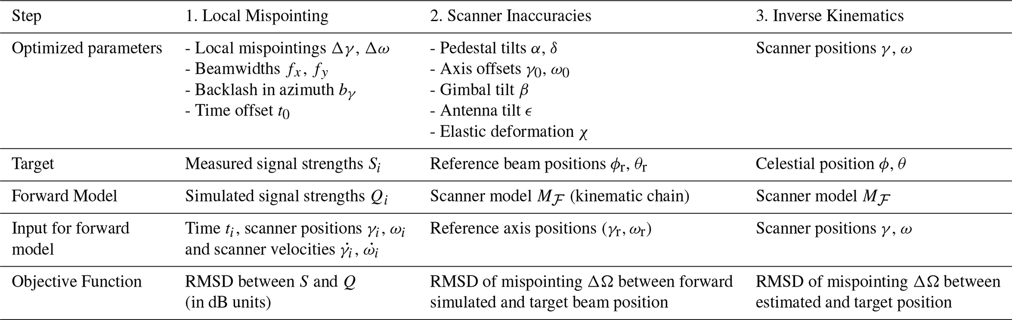
Table 1 Overview of the optimized parameters in each step. The steps are illustrated in Fig. 1.

2.2.1 Sun Scan Signal Simulation

Given a beam and Sun position, the expected signal in the receiver is determined by the convolution of the antenna's receiving pattern with the Sun's emission pattern. By the reciprocity theorem of electromagnetics, the receiving and transmitting patterns of the antenna are identical. In the following, we therefore refer to both as the radar beamshape.

Huuskonen and Holleman (2007) assume that the convolved signal distribution follows a Gaussian function. This assumption is valid, if the beam opening angle is significantly broader than the Sun opening angle, but leads to inaccuracies for narrower beams. Therefore, we numerically simulate the expected signal based on the convolution of a discretized version of the sky and antenna patterns.

We assume that the Sun and beam positions differ only by a small angular offset ±ν.¹ This allows us to approximate the celestial hemisphere as locally flat and to transform both positions into a Cartesian reference frame centered on the beam direction (illustrated in Fig. 3).

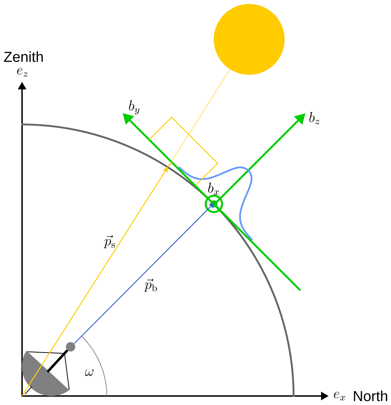
Figure 3 2D illustration of the definition of the beam centered coordinate frame (green). The radar beam pointing and antenna pattern are illustrated in blue, the Sun pointing vector and emission pattern are illustrated in yellow.

The beam-centered axes are defined as follows: the local b_z axis points radially outward along the beam, the local b_x axis lies orthogonal to b_z and e_z in the cross-elevation direction, and the local b_y axis completes the right-handed system.

$$\begin{array}{}\text{(9)}& b_z=\left(\begin{array}{c}\cos {\mathit{\varphi }}_{\mathrm{b}}\cos {\mathit{\theta }}_{\mathrm{b}}\\ \sin {\mathit{\varphi }}_{\mathrm{b}}\cos {\mathit{\theta }}_{\mathrm{b}}\\ \sin {\mathit{\theta }}_{\mathrm{b}}\end{array}\right),b_x={\displaystyle \frac{e_z\times b_z}{|e_z\times b_z|}},b_y=b_z\times b_x\end{array}$$

The beamshape of a parabolic antenna can be expressed by a two-dimensional Airy pattern (Kraus, 1988). In the beam-centered system, this is described by Eq. (10), which contains the first-order Bessel function J₁.

$$\begin{array}{}\text{(10)}& G\left(r\right)=G_{\mathrm{0}}{\left({\displaystyle \frac{\mathrm{2}{J}_{\mathrm{1}}\left(r\right)}{r}}\right)}^{\mathrm{2}},r=\sqrt{{\left({\displaystyle \frac{x}{x_{\mathrm{0}}}}\right)}^{\mathrm{2}}+{\left({\displaystyle \frac{y}{y_{\mathrm{0}}}}\right)}^{\mathrm{2}}}\end{array}$$

The coefficients in Eq. (10) are defined as

$$\begin{array}{}\text{(11)}& x_{\mathrm{0}}={\displaystyle \frac{f_x}{\mathrm{2}{r}_{\mathrm{0.5}}}},y_{\mathrm{0}}={\displaystyle \frac{f_y}{\mathrm{2}{r}_{\mathrm{0.5}}}},r_{\mathrm{0.5}}=\mathrm{1.6163399}.\end{array}$$

f_x and f_y are the beam full widths at half maximum (FWHM) in the x and y directions, respectively, r_0.5 is the value where the main lobe has half the maximum value: G(r_0.5) = $\frac{G_{\mathrm{0}}}{\mathrm{2}}$. G₀ is chosen such that the integral over G is one.

In a first approximation, the solar emission in the microwave region can be modeled as a bivalued function (Selhorst et al., 2003),

$$\begin{array}{}\text{(12)}& H(x,y)=\left\{\begin{array}{ll}{H}_{\mathrm{0}}& \text{if}(x,y)\text{lies outside the solar disk},\\ H_{\mathrm{1}}& \text{if}(x,y)\text{lies inside the solar disk},\end{array}\right.\end{array}$$

where H₀ is the background sky brightness and H₁ the solar disk brightness. The Sun is represented as a circle of angular radius

$$\begin{array}{}\text{(13)}& r_{\mathrm{s}}=\arcsin \left({\displaystyle \frac{r_{\text{planetary}}}{d_{\text{S-E}}}}\right),\end{array}$$

with planetary solar radius r_planetary = 695 660 km (Haberreiter et al., 2008). In the process of developing SunscanPy, we included a factor to allow for changes in the solar disk brightness near the limb, but found no significant improvements in the fit quality. The Sun–Earth distance d_S-E varies by about 3 % throughout the year due to Earth's orbital eccentricity and is evaluated for the scan time using the Skyfield library (Rhodes, 2019). At 35 GHz, the electromagnetic thermal emission of the sky is at least 13 dB lower than the emission of the Sun at 5800 K. Since for the Mira35 system, the Sun emission is around 4 dB higher than the noise floor of the receiver, this sky emission cannot be detected and is set to H₀ = 0. Figure 4 illustrates G(x,y) and H(x,y) in the beam-centered coordinate system.

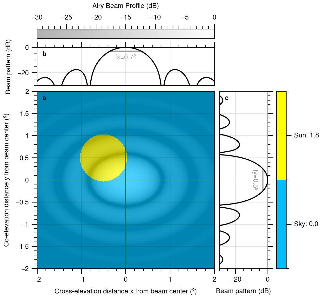
Figure 4 (a) Illustration of the Sun and sky emission pattern in beam centered coordinates, as “seen” by the radar. The background consists of just two emission values: the Sun (yellow) and the sky around (blue). This background is overlayed with an airy beampattern with f_x = 0.7, f_y = 0.5. The beampattern is illustrated by brighter and darker regions in the image. Darker means the radar is less sensitive in these regions. The top grey-white colorbar shows the sensitivity in dB. Panels (b) and (c) show horizontal and vertical cross sections of the beampattern. The expected signal detected by the radar is the summed product of background and beam pattern plus receiver noise. For this case, it yields a value of 0.8 dB, in between the brightness of the pure Sun and pure sky.

The simulated signal Q is then the convolution of the solar emission function H and the beamshape G plus the receiver noise H_n:

$$\begin{array}{}\text{(14)}& Q=H\times G+H_{\mathrm{n}}=H_{\mathrm{1}}\underset{\text{sundisk}}{\int }G(x,y)\mathrm{d}x\mathrm{d}y+H_{\mathrm{n}}.\end{array}$$

To evaluate Q, both H_n and H₁ must be determined. The receiver noise H_n can be measured directly by pointing the antenna sufficiently far from the Sun, i.e. by at least one expected beamwidth plus the pointing uncertainty. The solar brightness H₁, however, cannot directly be measured. Instead, it is inferred from the maximum measured signal S_max. Assuming that S_max originates from a beam direction close to the center of the solar disk, we can solve Eq. (14) for H₁:

$$\begin{array}{}\text{(15)}& H_{\mathrm{1}}={\displaystyle \frac{S_{max}-H_{\mathrm{n}}}{{\int }_{\text{centered sundisk}}G\mathrm{d}x\mathrm{d}y}}.\end{array}$$

This approach implies that the simulated signal at the disk center is by construction equal to S_max. Thus, the beam shape influences only the relative decay of the signal from the Sun's center towards the edge. A narrow beam produces a sharp transition between Sun and sky, while a wide beam yields a smoother decay.

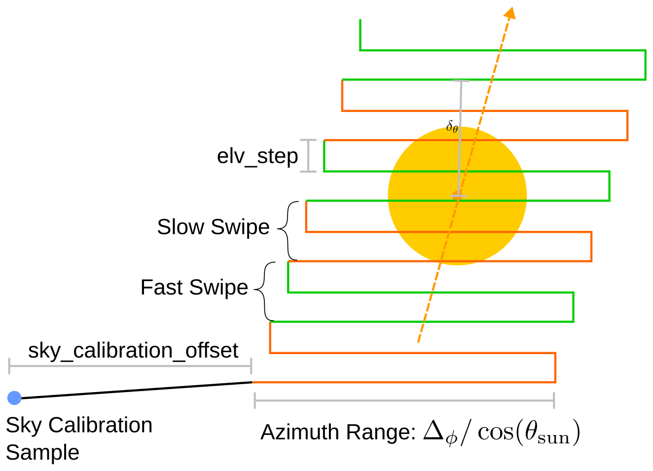
2.2.2 Proposed Scanning Pattern

Before conducting a Sun scan, we recommend adjusting the radar scanner to a moderate pointing precision, e.g. ν = 2°. This avoids the need to “search” the Sun across the entire celestial hemisphere. The adjustment can usually be performed visually or with a simple spirit level and compass. Once this preliminary alignment is completed, multiple samples are recorded within a region of angular size 2ν around the expected Sun position:

$$\begin{array}{}\text{(16)}& \mathit{\gamma }\in \left[{\mathit{\varphi }}_{\mathrm{s}}-\mathit{\nu },{\mathit{\varphi }}_{\mathrm{s}}+\mathit{\nu }\right],\mathit{\omega }\in \left[{\mathit{\theta }}_{\mathrm{s}}-\mathit{\nu },{\mathit{\theta }}_{\mathrm{s}}+\mathit{\nu }\right].\end{array}$$

The specific scanning pattern used within this region is not critical, since all sample tuples $(t_i,{\mathit{\gamma }}_i,{\mathit{\omega }}_i,\dot{{\mathit{\gamma }}_i},\dot{{\mathit{\omega }}_i},S_i)$ are treated independently. In practice, rectangular or rhombus-shaped “zigzag” scans are often employed. However, any pattern is acceptable provided that the following criteria are satisfied:

• 1.

  Coverage of the solar disk. The data must contain some measurements with the beam probing the solar disk's central region. If this is not the case, the search region ν must be enlarged.

• 2.

  Measurement of background sky noise. At least one sample must be taken sufficiently far from the Sun to record the receiver noise H_n. As a rule of thumb, this can be achieved at an azimuth offset of at least ν + f_x, i.e. at least the uncertainty in radar pointing plus the expected beamwidth (including sidelobes).

• 3.

  Use of multiple azimuth velocities. Ideally, the scan should include at least two different azimuth velocities. Since mechanical backlash depends only on the velocity sign, this enables the setup of two independent equations, which allow simultaneous estimation of both the backlash b_γ and the timing offset t₀:

  $$\begin{array}{}\text{(17)}& \begin{array}{c}{b}_{\mathit{\gamma }}\text{sign}\left(\dot{{\mathit{\gamma }}_{\mathrm{1}}}\right)+t_{\mathrm{0}}\dot{{\mathit{\gamma }}_{\mathrm{1}}}=b_{\mathit{\gamma }}+t_{\mathrm{0}}\dot{{\mathit{\gamma }}_{\mathrm{1}}},\\ b_{\mathit{\gamma }}\text{sign}\left(\dot{{\mathit{\gamma }}_{\mathrm{2}}}\right)+t_{\mathrm{0}}\dot{{\mathit{\gamma }}_{\mathrm{2}}}=b_{\mathit{\gamma }}+t_{\mathrm{0}}\dot{{\mathit{\gamma }}_{\mathrm{2}}}.\end{array}\end{array}$$

Apart from these requirements, the absolute axis velocities, sampling rate, and ordering of samples may be chosen freely according to the capabilities of the scanner and the signal processing system. Appendix A presents our specific scan pattern in the form of pseudocode.

2.2.3 Reverse Scanning

Many scanner systems permit elevation angles greater than 90°. In such cases, most points on the celestial hemisphere can be reached by the scanner in two different configurations: a forward configuration with ω ≤ 90° and a reverse configuration with ω > 90° (Fig. 5).

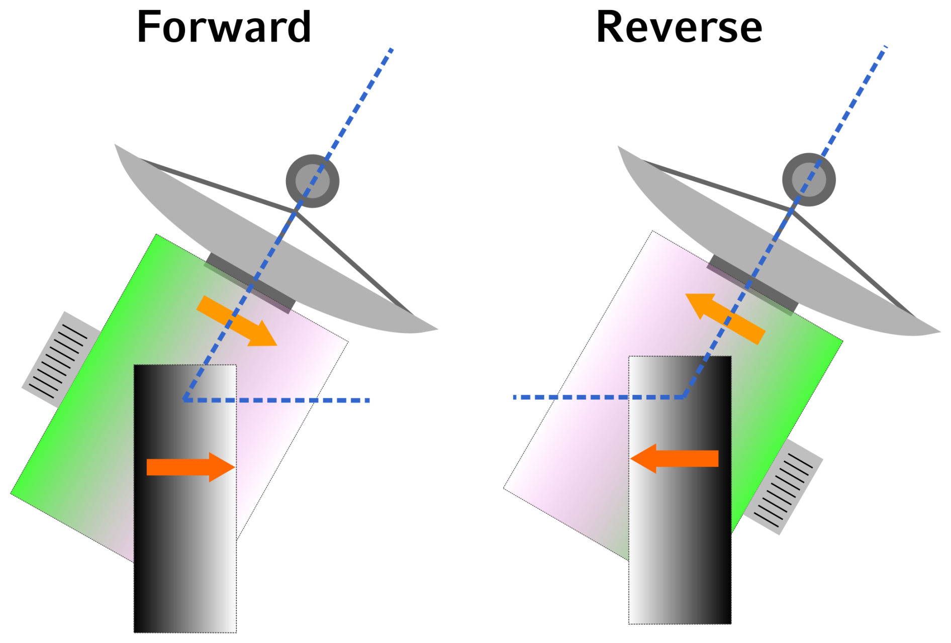
Figure 5 Illustration of the forward and reverse configuration of a two axis scanner. In both cases, the scanner points to the same location in the sky. However, in the reverse configuration, the scanner has turned by 180° in azimuth and the elevation angle (angle between the dashed, blue lines) is over 90°. The color gradients and arrows illustrate the orientation of the pedestal and scanner box.

Assuming an ideal scanner M_ℐ, forward and reverse positions are related by a rotation of 180° in azimuth combined with the complementary elevation:

$$\begin{array}{}\text{(18)}& {\mathit{\gamma }}^{\prime }=\mathit{\gamma }+\mathrm{180}\mathit{°},{\mathit{\omega }}^{\prime }=\mathrm{180}\mathit{°}-\mathit{\omega }.\end{array}$$

Performing Sun scans in both forward and reverse configurations is advantageous because it allows to resolve ambiguities in the scanner parameters. For instance, consider the case where a positive elevation mispointing Δω is observed, meaning the radar is pointing above the Sun. This deviation could originate either from an elevation axis offset or from a tilt of the scanner pedestal. In the reverse configuration, however, the two effects manifest differently: a pedestal tilt still produces a positive Δω, whereas an elevation offset causes a sign flip, leading the radar to point below the Sun. The reverse scan must satisfy the same requirements as the forward scan regarding coverage of the solar disk, measurement of sky noise, and inclusion of multiple scanning velocities.

2.3 Step 2: Estimate Scanner Inaccuracies

A single Sun scan provides information only about the local mispointing in one specific region of the sky. However, in other regions the mispointing may differ, depending on the specific inaccuracies of the scanner introduced in Sect. 2.1. To estimate these inaccuracies systematically, we implemented the forward model M_𝒫(γ,ω) as a kinematic chain using ikpy, a Python library for robotics and inverse kinematics (Manceron, 2024). The kinematic chain consists of four links: Origin, Azimuth joint, Elevation joint, and Antenna. Each link defines a rotated coordinate frame relative to the previous one, with the rotations depending on the parameters α, δ, β, ϵ, $\stackrel{\mathrm{̃}}{\mathit{\gamma }}$, and $\stackrel{\mathrm{̃}}{\mathit{\omega }}$. The effects of backlash b_γ, time offset t₀, angle offsets γ₀ and ω₀, as well as structural flexibility χ, are combined into the effective angles $\stackrel{\mathrm{̃}}{\mathit{\gamma }}$ and $\stackrel{\mathrm{̃}}{\mathit{\omega }}$.

A single Sun scan is not sufficient to unambiguously determine all parameters in 𝒫. For example, when scanning the Sun in the South, no information can be inferred about a potential East-West pedestal tilt α. To resolve such ambiguities, Sun scans at multiple positions across the sky are required, ideally covering the course of a full day in the summer months. Each Sun scan yields a pair of referenced coordinates (γ_r, ω_r) in the scanner system and the corresponding celestial reference coordinates (ϕ_r, θ_r).

For a given set of estimated parameters ℱ, we define an objective function based on the mispointing angle between the predicted beam position and the celestial reference position:

$$\begin{array}{}\text{(19)}& \mathrm{\Delta }\mathrm{\Omega }\left(M_{\mathcal{F}}({\mathit{\gamma }}_{\mathrm{r}},{\mathit{\omega }}_{\mathrm{r}}),({\mathit{\varphi }}_{\mathrm{r}},{\mathit{\theta }}_{\mathrm{r}})\right).\end{array}$$

The objective is defined as the RMSD of the mispointing across all referenced pairs:

$$\begin{array}{}\text{(20)}& O=\sqrt{{\displaystyle \frac{\mathrm{1}}{N}}\sum _{i=\mathrm{1}}^N\mathrm{\Delta }{\mathrm{\Omega }}_i^{\mathrm{2}}}.\end{array}$$

Minimizing this objective yields the set of parameters ℱ that best explains the observed radar pointing across all Sun scans. To carry out the minimization, we employ a two-step strategy: first, a three-point brute-force search provides reasonable starting values; second, a Nelder-Mead simplex optimization minimizes the objective (Gao and Han, 2010).

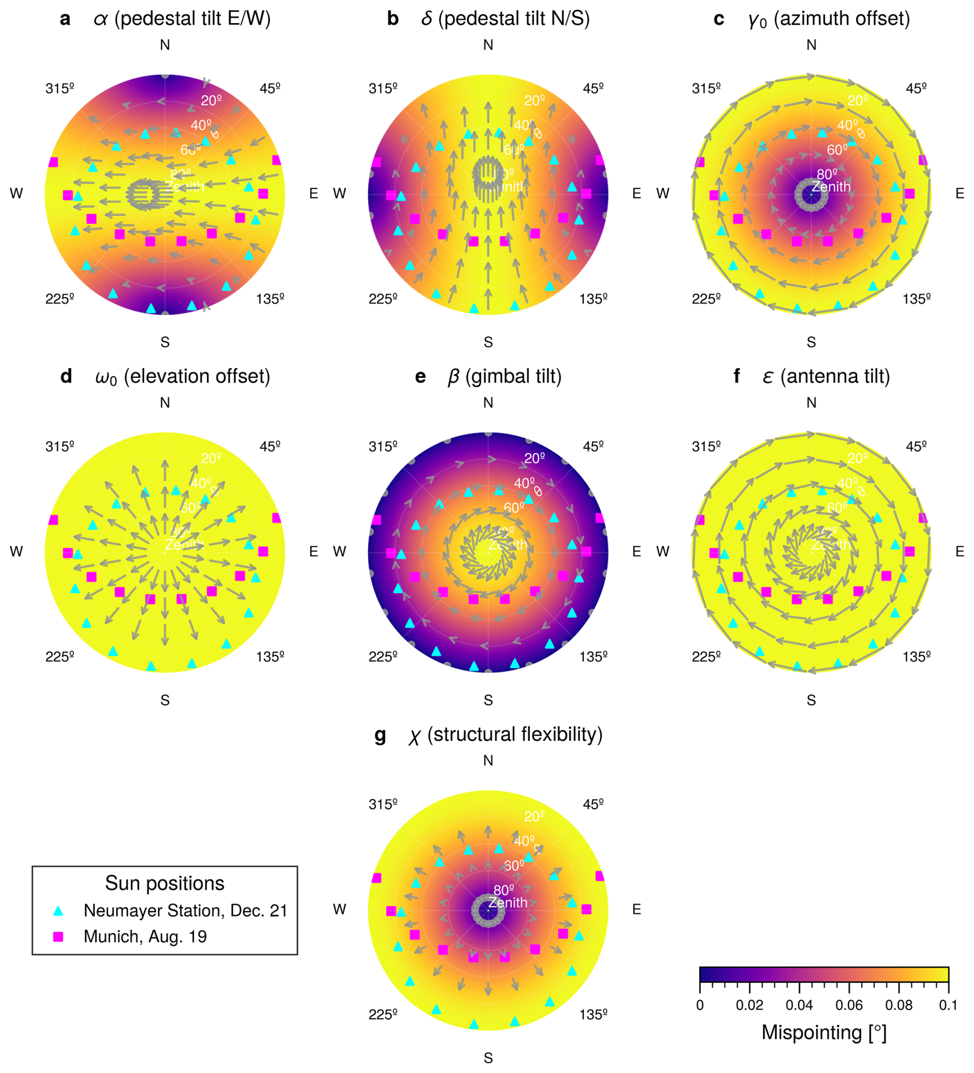
Global optimization in a high-dimensional parameter space is challenging, and simultaneous fitting of all parameters can cause the optimizer to become trapped in local minima. We found that sequential fitting, leveraging the specific mispointing signatures of each parameter, avoids this issue. Figure 6 shows the mispointing caused by each static scanner parameter over the celestial hemisphere. In our approach, previously fitted parameters are held fixed as best guesses in subsequent steps:

• 0.

  Backlash b_γ and time offset t₀. As described in Sect. 2.1, the dynamic parameters are assumed constant across the sky and can be estimated from a single Sun scan. We recommend averaging the results from multiple scans.

• 1.

  Azimuth offset γ₀ and antenna tilt ϵ. Near the horizon, azimuth mispointing Δγ can only be caused by γ₀ and ϵ (Fig. 6c and f). The contributions differ between forward and reverse scans: γ₀ produces the same sign in both, while ϵ produces opposite signs in forward and reverse (compare e.g. Figs. 6f and A1f).

• 2.

  East-West tilt α and elevation offset ω₀. Near the horizon in the East or West, elevation mispointing Δω can only be caused by East-West pedestal tilt α or elevation offset ω₀ (Fig. 6a and 6d). In analogy to the previous step, forward and reverse scans allow these effects to be distinguished.

• 3.

  North-South tilt δ and gimbal tilt β. At high elevation in the South (or North in the Southern Hemisphere), elevation mispointing Δω can be caused by North-South pedestal tilt δ or by ω₀ (Fig. 6b and 6d), with the latter already known from step (2) β causes mainly an azimuth offset Δγ, but can also have a contribution to Δω (Fig. 6e).

• 4.

  α, δ, β, ϵ, γ₀, ω₀, χ. Using the previous results as initial guesses, all parameters are jointly re-optimized against the full set of reference positions. At this stage, the flexibility parameter χ is included to account for residual elevation mispointings. Unlike α, δ, or ω₀, the effect of χ on the elevation mispointing depends on the absolute elevation (Fig. 6g).

Given a list of reference positions, the SunscanPy Python implementation automatically identifies the relevant sky regions and performs the sequential fitting procedure.

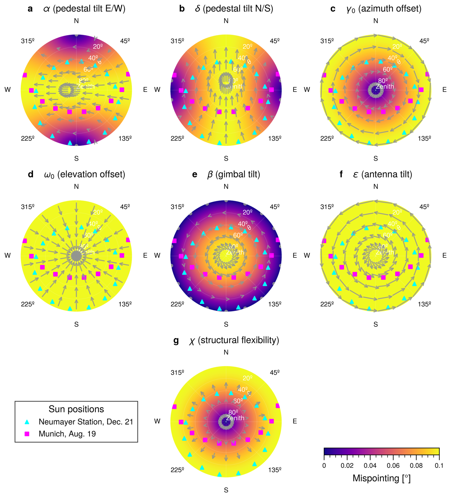
Figure 6 Mispointing caused by the static scanner parameters, as a function of position in the sky. Each panel shows the effect of a change in the corresponding parameter of 0.1° (χ: −0.1°), the other parameters are kept at 0.0°, respectively. Shown is the forward scanner configuration. The markers show the path of the Sun for Munich and an Antarctic location (Neumayer III station at 70°40^′ S, 008°16^′ W). The arrows show the direction and magnitude of the mispointing (magnitudes enhanced). Reading example for panel (d) An elevation offset of 0.1° causes a constant mispointing of 0.1° everywhere in the sky (colormap). The mispointing is always directed towards zenith (arrows).

2.4 Step 3: Inverse Kinematics

Once an estimate of the pan-tilt system parameters ℱ is available, misalignments can either be corrected mechanically – for example, by leveling the scanner pedestal – or compensated for in software. The latter requires inverting the forward model M_ℱ, such that for a desired celestial position (ϕ, θ), the corresponding scanner axis positions (γ, ω) are determined:

$$\begin{array}{}\text{(21)}& (\mathit{\gamma },\mathit{\omega })=M_{\mathcal{F}}^{-\mathrm{1}}(\mathit{\varphi },\mathit{\theta }).\end{array}$$

This inversion can be performed numerically by minimizing the mispointing between the desired celestial coordinates and the beam position predicted by the forward model, i.e., by finding the scanner position (γ, ω) that minimizes

$$\begin{array}{}\text{(22)}& \mathrm{\Delta }\mathrm{\Omega }\left(M_{\mathcal{F}}(\mathit{\gamma },\mathit{\omega }),(\mathit{\varphi },\mathit{\theta })\right).\end{array}$$

The feasibility of such inversion depends on the specific set of parameters. For example, offsets in the azimuth or elevation encoders (γ₀,ω₀) can be compensated straightforwardly. By contrast, an antenna tilt ϵ renders the zenith position unreachable, as will be discussed further in Sect. 3.3.

To test whether the inversion is successful, the obtained scanner position (γ, ω) is inserted back into the forward model, and the resulting pointing is evaluated against the target celestial position:

$$\begin{array}{}\text{(23)}& \begin{array}{rl}& \mathrm{\Delta }\mathrm{\Omega }\left(M_{\mathcal{F}}\right(\mathit{\gamma },\mathit{\omega }),(\mathit{\varphi },\mathit{\theta }\left)\right)\\ & =\mathrm{\Delta }\mathrm{\Omega }\left(M_{\mathcal{F}}\right(M_{\mathcal{F}}^{-\mathrm{1}}(\mathit{\varphi },\mathit{\theta })),(\mathit{\varphi },\mathit{\theta }\left)\right)\stackrel{!}{=}\mathrm{0}\mathit{°}.\end{array}\end{array}$$

3 Results

3.1 Step 1: Local Mispointing

Sun scans were carried out in August 2025 in Munich, southern Germany, using a Mira-35 Doppler cloud radar manufactured by Metek GmbH² (Görsdorf et al., 2015). The system operates in the Ka-band at 35.2 GHz and is equipped with a 1.2 m Cassegrain antenna. The radar is mounted on a steel platform at the top of the Munich Institute for Meteorology, supported by four adjustable anchor points. This setup provides a nearly unobstructed field of view down to 2° above the horizon. The antenna is mounted on a two-axis scanner with a nominal pointing precision of less than 0.1° in both azimuth and elevation. The signal transmission between the radar and control unit is performed via slip rings and a fiber-optic rotary joint, which allows unrestricted continuous rotation in azimuth. The scanner joints operate in a temperature- and humidity-controlled environment, ensuring stable mechanical performance during the measurements.

In principle, Sun scans can be performed even in cloudy conditions and with the radar still emitting radiation. In this case, the Sun signal is visible as enhanced receiver noise in target-free sections along the beam, preferably in the far range. We focus on the radar range gates between 3 and 27 km. We calculate the Sun signal as the average noise level in all cloud-free range gates. In general, for very low elevation angles, it is possible that there are not enough cloud-free far range gates, in which case the scan is excluded from analysis. We performed all scans on almost cloud-free days.

Figure 7a shows the measurements from a Sun scan performed on 19 August 2025 at 13:44 local time. The scan pattern follows the procedure described in Appendix B, with a radar averaging time of 0.3 s. Five samples (equivalent to 1.5 s) in the lower left corner were acquired to determine the background sky noise. The Sun is visible as an elongated region of enhanced signal strength. The two azimuth velocities used during the measurement, 0.2 and 0.4° s⁻¹, are clearly visible as more separated data points for faster azimuth velocity. Depending on the direction of azimuthal motion, a “zigzag” shift of the solar signal becomes visible, which indicates either mechanical backlash or a timing offset in the scanner system.

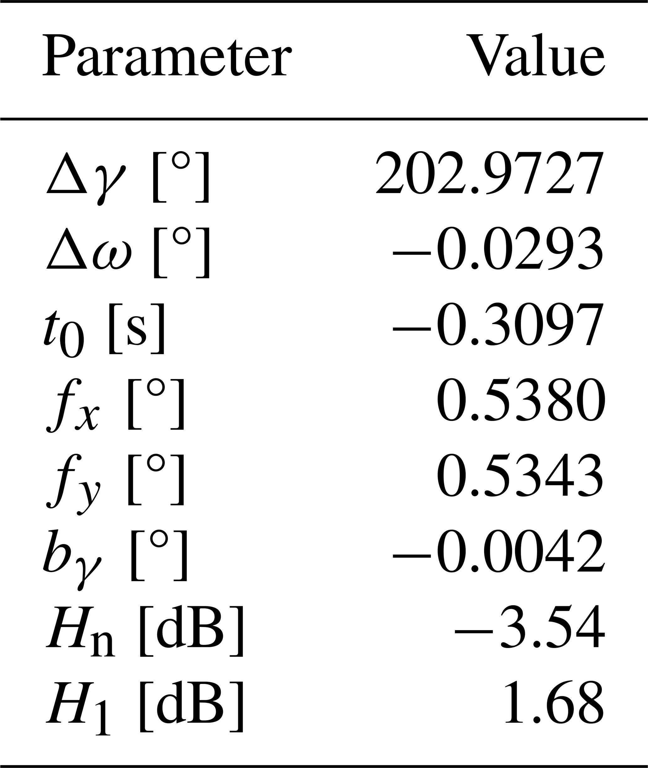
In Fig. 7b, the optimal fit of the simulated signal strength to the measured signal is shown. We see that the simulated samples reproduce both the overall shape of the solar response and the azimuth-dependent displacement. The corresponding best-fit parameters are listed in Table 2.

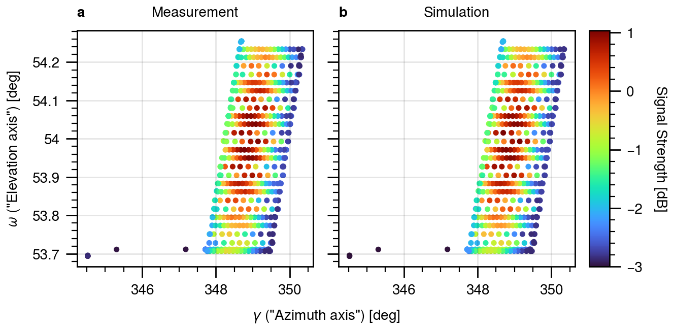
Figure 7 (a) Measurements of the Mira35 cloud radar when scanning the Sun. In azimuth, the scanner is alternating between two different azimuth velocities. (b) Simulated signal strength, using the parameters of Table 2. The parameters are determined as a best fit of the simulation to the measurements in panel (a).

Table 2 Parameters obtained from an optimal fit to the single Sun scan depicted in Figs. 7 and 8. Azimuth mispointing Δγ, elevation mispointing Δω, time offset between signal and scanner axis recording t₀, beam full width at half maximum in cross elevation f_x, beam full width at half maximum in co elevation f_y, scanner backlash b_γ, sky sample (receiver noise) H_n, Sun brightness H₁.

With these parameters, the Sun's position can be transformed into beam-centered coordinates. Figure 8a and b show the measured and simulated signal strength in this coordinate frame. Since the transformation incorporates the corrections for Δγ, Δω, t₀, and b_γ, the solar pattern appears undistorted and is centered at the origin. Figure 8c presents the residuals between measured and simulated signal strengths, with a mean deviation of 0.0013 dB (±0.1065 dB standard deviation).

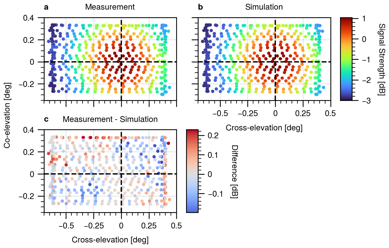
Figure 8 (a, b) Same as Fig. 7, but depicted in beam centered coordinates. (c) The difference between the signal strengths in panels (a) and (b).

Repeating such Sun scans throughout the day allows us to assess the variability of the derived parameters. Figure 9 summarizes these results as a function of solar elevation angle. Figure 9a and b show the beamwidths at half maximum in co- and cross-elevation directions. The cross-beamwidth is derived to approximately 0.55° across all scans, with a slight 0.01° decreasing tendency for higher solar elevation angles. The co-beamwidth is on average about 0.515°. There is an overall uncertainty of ±1.5 % in both beamwidths.

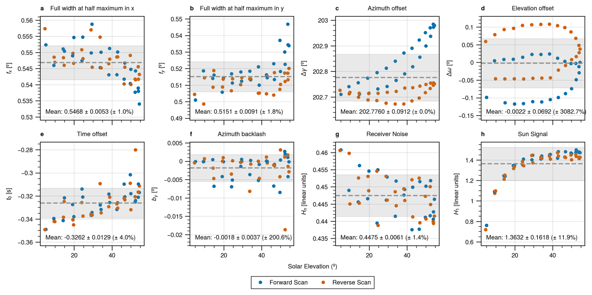
Figure 9 Variability of parameters over the course of one day, visualized as a function of solar elevation angle. The mean and standard deviation are indicated at the bottom of each panel and visualized as a dashed line and grey region, respectively.

Figure 9c and d display the mispointing corrections Δγ and Δω. Both exhibit systematic patterns over the course of the day, which will be further analyzed in Sect. 3.2. Figure 9e shows the time offset, with t₀ = −0.33 s, indicating that the recorded signal corresponds to the scanner position approximately one-third of a second earlier. Such a timeshift is expected, since the Mira35 radar stores the time at the end of the 0.3 s averaging interval, plus an additional processing time of the central processing unit (CPU). A positive correlation between Sun elevation and time offset is observed, amounting to a small change of approximately 0.03 s over the full day. We suspect that this might be due to solar heating and resulting changes in temperature of the system, affecting the CPU processing times of signal and axis encoders. Importantly, the time offset accounts for more than 95 % of the dynamic azimuthal mispointing in the scans. The contribution from gear backlash (Fig. 9f) is negligible at 0.002°.

The solar signal amplitude (Fig. 9g) increases strongly from 0.8 linear units (−1.0 dB) near the horizon to 1.5 linear units (1.8 dB) at 20° solar elevation, reflecting the reduced atmospheric path length and hence lower path integrated gas attenuation of the direct solar radiation. At higher elevations, the changes in path length and signal are less significant. At the same time, the signal of the sky sample decreases slightly from 0.45 linear units (−3.5 dB) by about 1 % to 0.445 linear units from horizon towards high noon.

3.2 Step 2: Scanner Inaccuracies

As described in Sect. 2.2, each Sun scan provides a referenced pair of scanner and celestial coordinates (γ_r,ω_r) and (ϕ_r,θ_r). With Sun scans distributed over the course of a full day, these data can be used to estimate the scanner inaccuracies following the procedure outlined in Sect. 2.3.

Figure 10a presents Sun scans performed on 11 and 12 August 2025. The figure shows both the actual beam positions (ϕ_b,θ_b) in the celestial hemisphere and the expected beam positions obtained from the scanner coordinates mapped into the sky using the identity scanner model,

$$\begin{array}{}\text{(24)}& ({\mathit{\varphi }}_I,{\mathit{\theta }}_I)=M_{\mathcal{I}}({\mathit{\gamma }}_{\mathrm{r}},{\mathit{\omega }}_{\mathrm{r}}).\end{array}$$

The comparison reveals large discrepancies between expected and actual beam positions, due to an uncorrected north angle γ₀ = 202.7°. After adding the northangle, the residual differences are much smaller (< 1°), as shown in Fig. 10b. For visibility, in Fig. 10b, the residuals are enhanced.

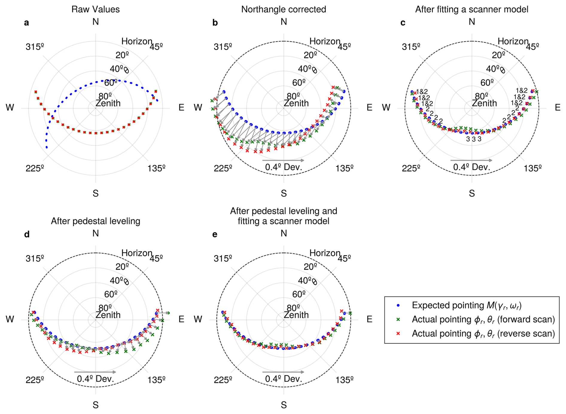
Figure 10 Difference between expected beam pointing (assuming a specific scanner model M, blue dots) and actual beam pointing (crosses), derived from multiple Sun scans over the course of one day. Since in panels (b) to (e), the differences are small, the actual beam pointing markers (crosses) are shifted into the direction of the deviation along the grey arrows. (a) Expected pointings are calculated from the raw axis positions and assuming an ideal scanner M_ℐ. (b) After correcting for the northangle in azimuth, the remaining differences are small and therefore enhanced in the plot. We see that in the southwest, for both the forward and reverse configuration, the radar points lower (closer to the horizon) than expected for an ideal scanner. The difference is about 0.2° (compare the length of the shift arrows with the 0.4° reference arrow). This is an indication for a southwest tilt of the scanner pedestal. (c) If the expected positions are calculated using the fitted scanner model M_ℱ1, the difference to the actual pointing is much smaller. (d) Situation after leveling the pedestal, assuming an ideal scanner M_ℐ. (e) After leveling the pedestal, with expected positions calculated using the fitted scanner model M_ℱ2.

Over the course of the day, the discrepancies exhibit a characteristic pattern. The largest deviations occur in the southwest, where the beam consistently points lower than expected. Since this effect is present in both forward and reverse scans, it indicates a pedestal tilt of approximately 0.2° towards the southwest.

We apply the sequential fitting procedure introduced in Sect. 2.3 to the data in Fig. 10a. Table 3 lists the optimal scanner parameters ℱ₁ obtained from this procedure. As expected, a positive α and negative δ confirm the southwest tilt. Compared to the pedestal tilt, the other inaccuracy parameters are about an order of magnitude smaller.³

Table 3 Scanner inaccuracies before and after manual leveling, as obtained from an optimal fit to multiple Sun scans. Azimuth offset γ₀, elevation offset ω₀, West-East pedestal tilt α, North-South pedestal tilt δ, gimbal tilt β, antenna tilt ϵ, signal-scanner time offset t₀, scanner backlash b_γ, elastic elevation deformation χ.

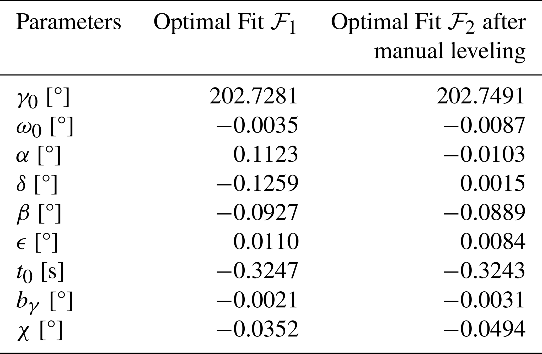
Figure 10c shows the expected scanner positions when the optimal parameters ℱ₁ are taken into account. The numbers next to the points in Fig. 10c indicate which samples are used for which step of the sequential fit, as presented in Sect. 2.3. Relative to Fig. 10b, the discrepancies are reduced by a factor of seven, yielding an average residual of only 0.02°. The remaining deviations are likely caused by effects not explicitly represented in the scanner model, such as position-dependent offsets, nonlinear elastic deformations, or differential thermal expansion of the steel support structure during the day.

With precise knowledge of the pedestal misalignment, we can proceed to correct it mechanically. Our radar is mounted on four adjustable screws arranged in a 977 mm by 1328 mm rectangle. Each full turn of a screw raises the corresponding corner by 2 mm, enabling fine adjustments. Figure 10d presents the results from a second series of Sun scans after adjusting the feet to compensate for the pedestal tilt. The remaining discrepancies are now dominated by other scanner inaccuracies, such as motor offsets, gimbal tilt β, and antenna tilt ϵ. As a consistency check, we re-estimated the optimal scanner parameters ℱ₂ from these new scans. The results, shown in Table 3 (second column), confirm that the pedestal is now aligned to within 0.01°, while the other parameters remain similar to their previous values. Taking M_ℱ2 as the basis for the expected pointing in Fig. 10e, the remaining discrepancies almost vanish and we get a similar agreement between expectation and measurement as in Fig. 10c.

3.3 Step 3: Inverse Kinematics

Instead of correcting the pointing errors mechanically, the ability to invert the scanner model M_𝒫 allows for an automatic correction in software. For example, if the radar is required to point to $(\mathit{\varphi }=\mathrm{0}\mathit{°},\mathit{\theta }=\mathrm{30}\mathit{°})$ in the sky, the corresponding scanner coordinates according to the fitted parameter set ℱ₁ are:

$$\begin{array}{}\text{(25)}& \begin{array}{rl}& M_{\mathcal{F}\mathrm{1}}^{-\mathrm{1}}(\mathit{\varphi }=\mathrm{0}\mathit{°},\mathit{\theta }=\mathrm{30}\mathit{°})\\ & =\left\{\begin{array}{ll}\mathit{\gamma }=\mathrm{157.30}\mathit{°},& \mathit{\omega }=\mathrm{29.91}\mathit{°},\\ \mathit{\gamma }=\mathrm{337.38}\mathit{°},& \mathit{\omega }=\mathrm{150.10}\mathit{°}.\end{array}\right.\end{array}\end{array}$$

The two solutions correspond to the forward and backward scanner configurations. Both solutions account for the complete set of inaccuracies represented in the scanner model. For cloud radar applications, the zenith position is typically the most critical. In this case, the inversion yields:

$$\begin{array}{}\text{(26)}& \begin{array}{rl}& M_{\mathcal{F}\mathrm{1}}^{-\mathrm{1}}(\mathit{\varphi }=\mathrm{0}\mathit{°},\mathit{\theta }=\mathrm{90}\mathit{°})\\ & =\left\{\begin{array}{ll}\mathit{\gamma }=\mathrm{171.06}\mathit{°},& \mathit{\omega }=\mathrm{89.85}\mathit{°},\\ \mathit{\gamma }=\mathrm{47.47}\mathit{°},& \mathit{\omega }=\mathrm{90.15}\mathit{°}.\end{array}\right.\end{array}\end{array}$$

At zenith, the prescribed azimuth ϕ = 0° is irrelevant for the pointing accuracy. The scanner azimuth positions γ listed in Eq. (26) were chosen to optimize the final pointing.

Figure 11a and b illustrate the corrections required to be added to the scanner coordinates γ and ω, respectively, to achieve perfect pointing across the full celestial hemisphere. Figure 11a is dominated by the system's north angle of 157.3°. Near zenith, the azimuth corrections increase, reflecting the reduced effectiveness of azimuth corrections at high elevation angles. Figure 11b is dominated by the southwest tilt of the pedestal: in the southwest, the elevation axis must be increased by about 0.2°, while in the northeast it must be reduced by roughly 0.1°.

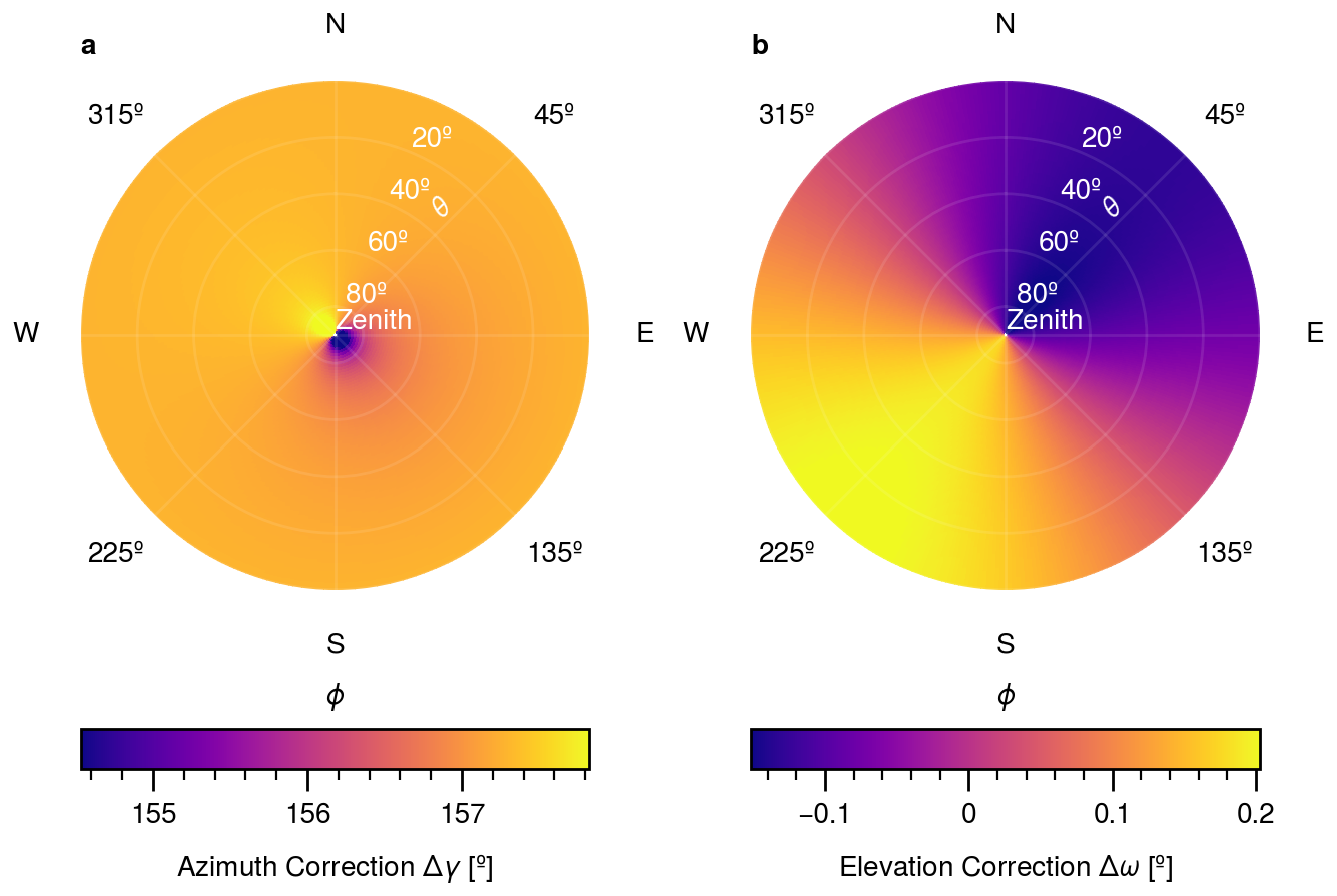
Figure 11 Corrections to be added to the scanner azimuth and elevation axis position in order to achieve perfect beam pointing accuracy, for all locations of the celestial hemisphere. (a) Azimuth correction. (b) Elevation correction.

It should be noted that inverse kinematics does not always allow for complete correction. Certain scanner configurations restrict accessibility to specific sky regions. For illustration, consider the extreme case where the dish is tilted by ϵ = 90°, effectively aligning the beam with the elevation axis. In this configuration, the elevation motor no longer affects the beam pointing, making it obviously impossible to reach the zenith position. Figure 12a shows the hypothetical case of an antenna tilt of ϵ = 10°. Here, the maximum achievable beam elevation is 80°, leaving the zenith position unreachable. Above this limit, the residual mispointing after inverse kinematics correction increases continuously, reaching up to 10° at zenith.

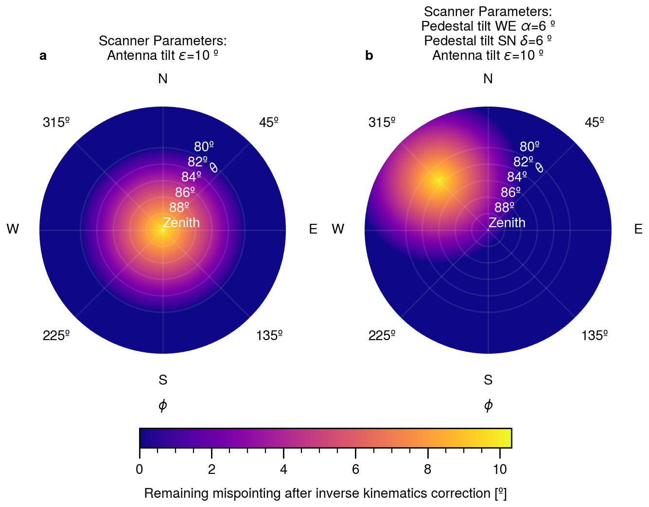
Figure 12 Simulated pointing deviation from desired location after inverse kinematics correction for two different scanner configurations. (a) A perfectly leveled scanner with an antenna tilt of 10°. (b) Like panel (a), but with the scanner pedestal tilted towards North and West by 6°.

A straightforward solution for Doppler cloud radars is to deliberately shift the unreachable polar region away from zenith by tilting the pedestal. Figure 12b illustrates this effect for a virtual scanner tilted by 6° towards both the west and north. The unreachable region is displaced accordingly, and zenith can again be reached with nearly perfect accuracy. In fact, the same result would be achieved for a sufficiently large pedestal tilt into any direction. This leads to the paradoxical effect that with the ability to perform inverse kinematics corrections, a perfectly leveled pedestal represents the least favorable configuration, as it maximizes the risk of an unreachable zenith.

4 Discussion

4.1 Dependence on Latitude and Seasonality

As described in Sect. 2 and Fig. 1, the Sun scan method requires multiple Sun scans at different positions in the sky. However, the accessible positions may be restricted by a limited solar path, for example at high latitudes or during winter months, or by radar-specific constraints such as surrounding obstacles or mechanical limitations of the scanner.

To assess the impact of such restrictions on the applicability of the method, Fig. 6 shows the mispointing caused by a deviation of 0.1° in each scanner parameter across all sky positions. In general, a parameter can only be inferred from Sun scans if measurements are available from sky regions where the pointing is sensitive to that parameter. The markers in each panel illustrate the Sun positions for Munich and a high-latitude site (Neumayer III station, 70°40^′ S, 008°16^′ W). For the polar site, the Sun traverses at least one sensitive region for all parameters except the gimbal tilt β. Hence, even in polar regions with only low solar elevation angles available, we expect that all parameters except β can be estimated.

For campaigns and mobile radars, the pedestal tilts α and δ are likely the most relevant parameters. As described in Sect. 2.3, their estimation requires only samples close to the horizon in the West and East, or North and South, respectively. However, during polar winter conditions, when the Sun remains confined to the North or South, α cannot be reliably estimated because no sensitivity exists near the horizon in the North or South (Fig. 6a).

These considerations apply analogously to local obstacles or mechanical constraints. In the latter case, reverse scans may not be feasible. Consequently, certain parameter pairs, such as γ₀ and ϵ, cannot be determined independently (see also Sect. 2.3). In such situations, we recommend fixing one parameter and excluding it from the fit. For example, the gimbal tilt β and the antenna tilt ϵ may be assumed small and prescribed according to manufacturer specifications.

4.2 Pointing Uncertainty

Figure 9 already provides a measure of the relative uncertainty of the Sun scan parameters by showing the variability of repeated scans throughout the day. Beyond this variability, sources of absolute bias must also be considered.

A potential source for uncertainty is the accuracy of the solar position algorithm. We compared four different algorithms. Skyfield (Rhodes, 2019), Sunpy (The SunPy Community et al., 2020) and PySolar (Stafford, 2021) are free and open source Python modules. SolCalc (NOAA Global Monitoring Laboratory, 2025) is the solar position calculator from the US National Oceanic and Atmospheric Administration. We found general agreement in the solar azimuth and elevation of better than 0.02° between the libraries. The main cause for this difference is whether refraction is considered and how a correction is implemented. For the calculations in this manuscript and SunscanPy, we rely on the geometrical (i.e. not refraction corrected) position provided by Skyfield. We then apply the microwave refraction formula proposed by Huuskonen and Holleman (2007). Their coefficients were fitted to simulations of the Starlink positional astronomy library (Currie et al., 2014), which uses the refractivity model from Rueger (2002a). The Starlink implementation is generally valid for microwave radiation in the GHz range, with a reported accuracy better than 1^′′. It does not include an explicit wavelength dependency. According to Rueger (2002b), dispersion of the refractive index would be most relevant near oxygen and water vapor resonance lines, which are deliberately outside of the frequency bands used by weather and cloud radars. Figure 13a shows the correction to the geometric solar elevation as a function of Sun elevation. The effect is largest near the horizon, but already at elevations above 10°, the correction remains below 0.1°. The dominant source of uncertainty in this parameterization is atmospheric humidity. Figure 13b illustrates how the apparent solar elevation changes when relative humidity increases from 0 % to 50 %, and from 50 % to 85 %. Above 10°, the associated effect is less than 0.01°. For the calculations in the previous sections, we assumed a constant humidity of 50 %. While future refinements could incorporate vertical humidity profiles from radiosonde measurements, this level of detail is not necessary to achieve an absolute calibration accuracy well below 0.1°. This conclusion is confirmed by sensitivity tests: repeating our calculations with 85 % humidity altered the derived scanner parameters by in general less than 10^′′.

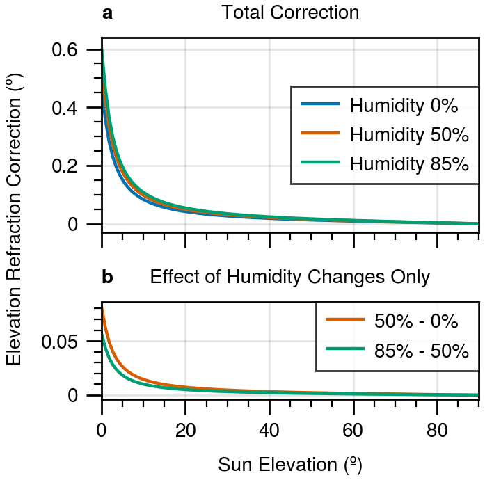
Figure 13 Apparent shift in elevation of the solar disk due to atmospheric refraction of GHz radio waves, as a function of solar elevation. (a) Absolute shift. (b) Differences between the curves in panel (a), with the 0 % humidity curve taken as a reference.

In order to estimate the Sun position accurately, precise timing is important. As described in Sect. 2.1, we use different azimuth velocities to estimate the relative time offset between signal and scanner encoder readings. However, this method cannot correct for an absolute time offset being present in signal processor and scanner encoder alike. Absolute time offsets will cause an apparent mispointing, which is always directed along the trajectory of the Sun. Depending on the latitude and season, it may therefore be possible to derive an absolute time offset from the characteristic misalignment pattern of multiple Sun scans. Nevertheless, for practical applications, we recommend simply synchronizing the time of the radar before a Sun scan calibration. Using for example GPS time or the standard network time protocol (NTP) synchronization available in modern operating systems, an accuracy of 100 ms or better should be easily achieved (Mills, 1994). From sensitivity tests, we found time shifts of 1 s to cause in general less than 10^′′ shift in the derived scanner parameters.

5 SunscanPy Python Implementation

The calibration framework developed in this study is provided as an open-source Python library SunscanPy. The library is written in a modular, object-oriented style and reads data in the form of one-dimensional numpy arrays. This facilitates the inclusion of the methods into existing data pipelines and operational environments. Figure 14 provides a schematic overview of the data processing. This processing chain was also used for the results in this study. Together with the library, we provide two detailed tutorial notebooks covering signal estimation and scanner estimation, guiding users through the full solar pointing calibration process. In addition, the library includes various utility functions for atmospheric refraction correction, solar position calculation, Sun scan data plotting, and an interactive 3D visualization of the scanner geometry. For usage, the recommended starting point is the project homepage at https://github.com/Ockenfuss/sunscanpy (last access: 24 April 2026), where the tutorial notebooks are also provided.

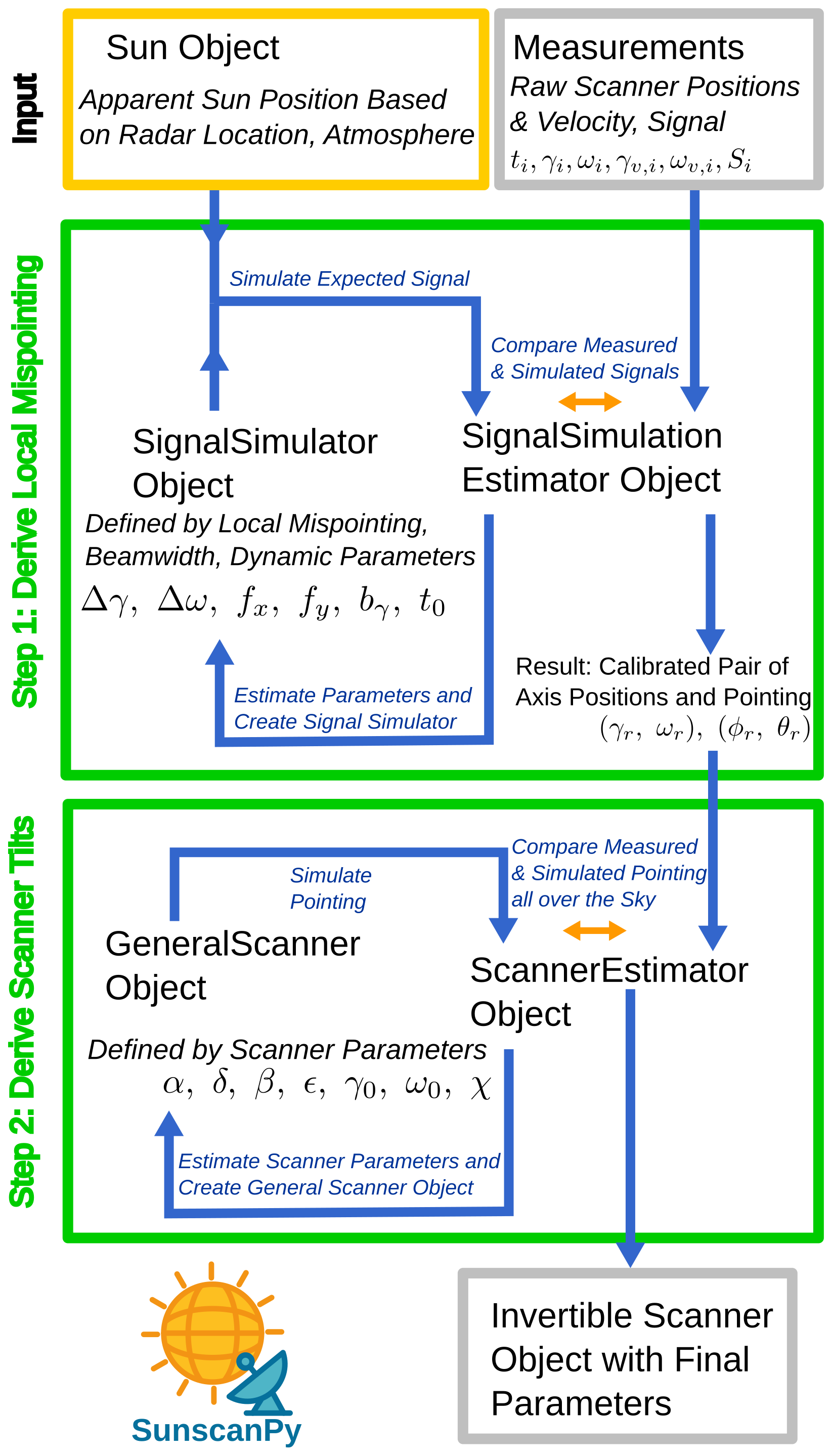
Figure 14 Overview of the modules and dataflow in the SunscanPy Python library. The two green boxes represent the two major processing steps in SunscanPy and correspond conceptually to step one and two in Fig. 1, respectively. The core of each step is a loop (as illustrated by the blue arrows), in which the parameters of an object are fitted iteratively to the given data. In step one, the data consists of values (radar measurements and scanner position) of a single sunscan and the parameters are the local mispointing, beamwidth and dynamic coefficients. In step two, the data consists of the referenced coordinate pairs produced by step one and the parameters are the scanner coefficients. Please refer to the methods in Sect. 2 and the list of symbols at the end of this publication for a definition of the parameters in the figure.

6 Conclusions

We have presented a generic theory and workflow for radar pointing calibration using the Sun as a reference source. The procedure is structured into three major steps: (i) recording and evaluation of individual Sun scans, (ii) derivation of scanner inaccuracies, and (iii) correction of these inaccuracies. In total, the method allows the derivation of 13 distinct parameters. These include the radar beamwidth in co- and cross-elevation directions, the scanner pedestal tilt, axis misalignments, encoder offsets, gear backlash, and the receiver-scanner time offset. Our results demonstrate that, with this approach, a pointing accuracy on the order of 0.01° can be achieved.

Although the workflow is demonstrated here with a Mira-35 cloud radar, the methodology has been deliberately designed to be radar-agnostic. The procedures apply to any instrument equipped with a parabolic antenna mounted on a two-axis scanner, whether the radar is a cloud research radar or used for weather surveillance.

To facilitate the application, we provide a novel open-source Python package SunscanPy, which contains a suite of tools together with comprehensive tutorials and example data for radar pointing calibration. We also discuss the possibility of fully automatic radar pointing calibration. SunscanPy implements an inversion method for the scanner model, enabling calculation of the scanner coordinates required to achieve a desired celestial pointing. This opens the possibility for active radar pointing calibration as an alternative to manual, mechanical adjustments: after performing Sun scans, a radar can infer its scanner misalignment and then compensate for any bias in subsequent measurements. Such functionality will be highly valuable for mobile radars, for example deployed in field campaigns, where uneven ground or snow may cause significant pedestal misalignment.

Stationary scanning radars likewise benefit from our workflow. SunscanPy makes it possible to monitor pointing accuracy over long time scales, or, if the scanner configuration is assumed to be stable over time, to retrospectively improve the pointing accuracy of existing datasets. For these reasons, we think that our tool will be of interest to network-level initiatives such as the European Aerosol, Clouds and Trace Gases Research Infrastructure (ACTRIS, Laj et al., 2024) or the U.S. Atmospheric Radiation Measurement (ARM, Mather and Voyles, 2013) program. Long-term cloud radar datasets are increasingly used to infer statistics of, for example, hydrometeor sedimentation velocities or vertical air motion (e.g., Kalesse and Kollias, 2013). Also new satellite missions, such as EarthCare, benefit from well-calibrated ground-based radar datasets to evaluate their novel Doppler velocity capabilities.

Last, but not least, while not investigated in this study, we believe that our methodology and the SunscanPy package can also be applied to other scanning, two-axis instruments like Sun photometers or microwave radiometers. Particularly step (ii) and (iii) of the workflow have the potential to be transferred with minor to no adaptations to those instruments.

Appendix A: Reverse Parameter Sensitivity

Figure A1 shows the effect of the static scanner parameters on the mispointing in the sky for the reverse scanner configuration.

Figure A1 Same as Fig. 6, but for the reverse scanner configuration. Note how the direction of the mispointing (arrows) changes for some of the parameters, compared to Fig. 6.

Appendix B: Implementation of a Sun Scan Pattern

As explained in Sect. 2.2.2, any scanning pattern which yields sufficient samples around the Sun can be evaluated. For practical applications, some patterns are more efficient in terms of scanning time and spatial resolution. Given the huge variety of hardware and programming languages used to control scanning weather and cloud radars, it is difficult to provide ready-to-run scripts for every radar. Instead, in Algorithm B1 we provide a pseudocode implementation of the scan pattern we used for our measurements. The only radar specific command in the pseudocode is move to, which steers the scanner to a given pair of axis positions. If such a command is available, it should be straightforward to implement a Sun scan in any programming language. Figure B1 illustrates the resulting pattern. Our code takes the movement of the Sun into account and dynamically follows the expected position of the solar disk. If the Sun is located at high elevations in the sky, the azimuth range and azimuth speed are enhanced to sample a constant solid angle in the sky. To perform a reverse scan, the only adaption is to exchange the move to function in Algorithm B1 with the move reverse function described in Algorithm B2.

Figure B1 Illustration of the scan pattern used in Fig. 7. Algorithm B1 gives an example how this can be implemented in code.

Algorithm B1 Sun scan pattern algorithm.

Require:

Δ_ϕ, Δ_θ, elv_step, speed_fast, speed_slow, sky_calibration_offset

Input parameters:

Δ_ϕ: Azimuth width of the search pattern

Δ_θ: Elevation width of the search pattern

elv_step: Step width in elevation

speed_fast: Speed in azimuth for the fast swipes

speed_slow: Speed in azimuth for the slow swipes

sky_calibration_offset: Additional offset in azimuth to measure the sky calibration sample

${\mathit{\varphi }}_{\mathrm{sun}},{\mathit{\theta }}_{\mathrm{sun}}\leftarrow \text{compute\_sun\_location()}$

$\text{azimuth\_factor}\leftarrow \mathrm{1}/\cos \left({\mathit{\theta }}_{\mathrm{sun}}\right)$

// correct the azimuth range for the elevation of the Sun

$\text{azimuth\_factor}\leftarrow min(\text{azimuth\_factor},\mathrm{4})$

// limit to avoid too large speeds and ranges if the Sun is close to zenith

${\mathrm{\Delta }}_{\mathit{\varphi }}\leftarrow {\mathrm{\Delta }}_{\mathit{\varphi }}\times \text{azimuth\_factor}$

$\text{speed\_fast}\leftarrow \text{speed\_fast}\times \text{azimuth\_factor}$

$\text{speed\_slow}\leftarrow \text{speed\_slow}\times \text{azimuth\_factor}$

$\text{sky\_calibration\_offset}\leftarrow \text{sky\_calibration\_offset}\times \text{azimuth\_factor}$

move to $({\mathit{\varphi }}_{\mathrm{sun}}-{\mathrm{\Delta }}_{\mathit{\varphi }}-\text{sky\_calibration\_offset},{\mathit{\theta }}_{\mathrm{sun}}-{\mathrm{\Delta }}_{\mathit{\theta }})$

// move to the sky calibration position

sleep(1)

// wait one second to measure some sky background values

${\mathit{\varphi }}_{\mathrm{sun}},{\mathit{\theta }}_{\mathrm{sun}}\leftarrow \text{compute\_sun\_location()}$

// update Sun position

${\mathit{\delta }}_{\mathit{\theta }}\leftarrow -{\mathrm{\Delta }}_{\mathit{\theta }}$

// current elevation of the beam relative to the (moving) sun

move to $({\mathit{\varphi }}_{\mathrm{sun}}-{\mathrm{\Delta }}_{\mathit{\varphi }},{\mathit{\theta }}_{\mathrm{sun}}+{\mathit{\delta }}_{\mathit{\theta }})$

// move to the exact starting position

iteration←0

while δ_θ<Δ_θ do

if iteration  mod  2=0 then

ϕ_v←speed_slow

else

ϕ_v←speed_fast

end if

move to $({\mathit{\varphi }}_{\mathrm{sun}}+{\mathrm{\Delta }}_{\mathit{\varphi }},{\mathit{\theta }}_{\mathrm{sun}}+{\mathit{\delta }}_{\mathit{\theta }})$ at speed ϕ_v

// move right

${\mathit{\varphi }}_{\mathrm{sun}},{\mathit{\theta }}_{\mathrm{sun}}\leftarrow \text{compute\_sun\_location()}$

// update Sun position

${\mathit{\delta }}_{\mathit{\theta }}\leftarrow {\mathit{\delta }}_{\mathit{\theta }}+\text{elv\_step}$

// update relative elevation

move to $({\mathit{\varphi }}_{\mathrm{sun}}+{\mathrm{\Delta }}_{\mathit{\varphi }},{\mathit{\theta }}_{\mathrm{sun}}+{\mathit{\delta }}_{\mathit{\theta }})$ at speed ϕ_v

// move up

move to $({\mathit{\varphi }}_{\mathrm{sun}}-{\mathrm{\Delta }}_{\mathit{\varphi }},{\mathit{\theta }}_{\mathrm{sun}}+{\mathit{\delta }}_{\mathit{\theta }})$ at speed ϕ_v

// move left

${\mathit{\varphi }}_{\mathrm{sun}},{\mathit{\theta }}_{\mathrm{sun}}\leftarrow \text{compute\_sun\_location()}$

// update Sun position

${\mathit{\delta }}_{\mathit{\theta }}\leftarrow {\mathit{\delta }}_{\mathit{\theta }}+\text{elv\_step}$

// update relative elevation

move to $({\mathit{\varphi }}_{\mathrm{sun}}-{\mathrm{\Delta }}_{\mathit{\varphi }},{\mathit{\theta }}_{\mathrm{sun}}+{\mathit{\delta }}_{\mathit{\theta }})$ at speed ϕ_v

// move up

$\text{iteration}\leftarrow \text{iteration}+\mathrm{1}$

end while

Algorithm B2 Move reverse function.

Require:

γ, ω

Input parameters:

γ: Desired forward azimuth position in the sky.

ω: Desired forward elevation position in the sky.

γ_reverse← (γ+180°) mod 360°

${\mathit{\omega }}_{\mathrm{reverse}}\leftarrow \mathrm{180}\mathit{°}-\mathit{\omega }$

move to (γ_reverse,ω_reverse)

Appendix C: List of Symbols

α	Pedestal tilt towards West or East
β	Gimbal tilt
bγ	Azimuth backlash
δ	Pedestal tilt towards North or South
ϵ	Antenna tilt
γ	Azimuth axis position
γ0	Azimuth axis offset
γr	Azimuth axis position, belonging to a referenced position in the sky (ϕr, θr)
$\dot{\mathit{\gamma }}$	Azimuth axis velocity
ω	Elevation axis position
ω0	Elevation axis offset
ωr	Elevation axis position, belonging to a referenced position in the sky (ϕr, θr)
$\dot{\mathit{\omega }}$	Elevation axis velocity
t0	Time offset between axis positioners and signal recorder
χ	Elastic elevation deformation
θ	Elevation angle (celestial coordinates)
ϕ	Azimuth angle (celestial coordinates)
ϕs	Solar azimuth position
θs	Solar elevation position
ϕb	Beam azimuth position
θb	Beam elevation position
ϕr	Azimuth position in the sky, providing the reference to a scanner position (γr, ωr)
θr	Elevation position in the sky, providing the reference to a scanner position (γr, ωr)
Δγ	Local azimuth mispointing
Δω	Local elevation mispointing
ΔΩ	Angular mispointing
fx	Beam full width at half maximum in cross-elevation direction
fy	Beam full width at half maximum in co-elevation direction
G	Antenna beam pattern function
H	Solar emission pattern function
H0	Sky brightness
H1	Solar disk brightness
Hn	Receiver noise level
Q	Simulated signal strength
S	Measured signal strength
rs	Angular radius of solar disk
M𝒫	Forward scanner model with parameters 𝒫
Mℐ	Ideal scanner model
𝒫	Set of scanner inaccuracy parameters
ℱ	Fitted scanner parameters
J1	First-order Bessel function
bx, by, bz	Beam-centered coordinate axes
x0, y0	Beam shape coefficients
r0.5	Radius where beam has half maximum value