Hybrid methodology for optimised water vapour mixing ratio profiles from Raman lidar measurements

This study presents a hybrid methodology to obtain high temporal resolution calibration constants for water vapour Raman lidar measurements, and posteriorly retrieve high-accuracy water vapour mixing ratio profiles. The hybrid method combines correlative measurements of collocated precipitable water vapour and Numerical Weather Prediction data to reconstruct the profile within the incomplete overlap region. The hybrid methodology is applied to the Raman lidar system, which operated at the EARLINET/ACTRIS station of the University of Granada, Spain, for the period 2009–2022. The system has been continuously updated to meet EARLINET/ACTRIS requirements for aerosol measurements, but the hybrid method has allowed tracking the impact of these changes on calibration constants for water vapour retrievals, and consequently to exploit water vapour mixing ratio profiles that were previously unavailable. The hybrid method was optimised for the Granada station by selecting Global Navigation Satellite System precipitable water vapour data as the most appropriate due to its better agreement with collocated and simultaneous radiosonde data (coefficient of determination of 0.95). Furthermore, the ERA5 reanalysis model was selected as the most appropriate because of its better temporal and spatial resolution and its accuracy when evaluated against radiosonde data. The advantages of the hybrid methodology were evaluated in comparison to traditional calibration methods such as those based on radiosondes or precipitable water vapour data assuming a constant water vapour mixing ratio in the incomplete overlap region. Although all methods generally provided good calibration constants, the hybrid method presented the best assessments under conditions where atmospheric layers were not well-mixed. Comparison with radiosonde data revealed excellent agreement, with a mean bias of −0.1 ± 0.3 g kg⁻¹, a standard deviation of 1.0 ± 0.4 g kg⁻¹ and a coefficient of determination of 0.87 across the entire period and vertical range (0–6 $\mathrm{km}\mathrm{a}.\mathrm{g}.\mathrm{l}.$). The most important result of this study is the ability to continuously evaluate calibration constants in a system that its configuration has been changing over 14 years of operation. This new methodology expanded the dataset from 31 initial cases using collocated radiosondes to more than 2000 values through the hybrid methodology. The posterior application of the hybrid methodology to all Raman lidar measurements enabled the generation of a comprehensive database of water vapour mixing ratio profiles for the entire period 2009–2022. Illustrative cases under different atmospheric conditions are presented to showcase the potential of Raman lidar measurements in monitoring water vapour and to investigate its role in climate dynamics and weather prediction.

1 Introduction

Water vapour is one of the most important constituents in the Earth's atmosphere due to its key role in determining the thermodynamic state of the atmosphere. It is considered the most important and variable greenhouse gas (Douville et al., 2021), accounting for about 60 % of the natural greenhouse effect under clear skies (Kiehl and Trenberth, 1997) and providing the largest positive feedback in model projections of climate change (Held and Soden, 2000). Moreover, changes in water vapour concentration can significantly affect radiative balance and energy transport mechanisms in the atmosphere (Whiteman et al., 1992; Ferrare et al., 2000; Niemeier et al., 2023), as well as photochemical processes (Haefele et al., 2008). Water vapour also contributes indirectly to the radiative budget through microphysical processes that lead to the formation and development of clouds, and by affecting the size, shape, and chemical composition of aerosol particles (Reichardt et al., 2012; Navas-Guzmán et al., 2019), thus modifying the role of aerosols in radiative forcing (DeTomasi and Perrone, 2003). All of these considerations imply that systematic and accurate observations of water vapour are required to achieve a comprehensive understanding of its role on local and global scales and ultimately improve climate projections (Foth et al., 2015).

Advances in remote sensing techniques have enabled more frequent measurements of precipitable water vapour (W), which is defined as the total atmospheric water vapour contained in a vertical column of unit cross section (American Meteorological Society, 2014). Most of these measurements exploit observations in water vapour absorption bands (e.g., sun/star photometry, Pérez-Ramírez et al., 2012, 2014, or microwave radiometry, Foth et al., 2015). These physical principles are also applied in satellite measurements of W, allowing observations in remote regions (Grossi et al., 2015; Roman et al., 2016; Pérez-Ramírez et al., 2019; Küchler et al., 2022). However, such measurements require clear skies. The Global Navigation Satellite System (GNSS) partially addresses this limitation, as it operates in most weather conditions (Bruyninx et al., 2019; Gong and Liu, 2021; Ding et al., 2022; Vaquero-Martínez et al., 2022; Yuan et al., 2023), extending W measurements at many stations around the world (Blewitt et al., 2018). Nevertheless, none of these measurement techniques can provide information on the vertical distribution of water vapour, which is critical because water vapour concentration typically varies by three orders of magnitude between the surface and the upper troposphere (Held and Soden, 2000; Tompkins, 2002). In this context, radiosondes (RS) are considered a reference method for determining water vapour content with high vertical resolution (World Meteorological Organization (WMO) et al., 2024). However, these measurements are spatially sparse and have a low temporal resolution, which depends on the launch frequency (Vaughan et al., 1988). Microwave radiometers (MWR) can partly solve this problem (Foth et al., 2015) but with low vertical resolution (Westwater et al., 2005), especially for upper troposphere water vapour measurements, and they are affected by the presence of clouds and rainfall (Turner et al., 2002; Foth et al., 2015). Despite this, W by MWR can be accurately estimated, allowing MWR to be used as a reference instrument to retrieve the total column concentration of water vapour (Turner et al., 2007; Cadeddu et al., 2013; Hocke et al., 2017).

Active remote sensing has proven to be an ideal technique for obtaining water vapour mixing ratio (r) profiles with high vertical and temporal resolution. The most common techniques used are Differential Absorption Lidar (DIAL) (e.g., Di Girolamo et al., 2020; Mariani et al., 2020) and Raman lidars (e.g., Whiteman et al., 1992; Guerrero-Rascado et al., 2008; Navas-Guzmán et al., 2014; Kulla and Ritter, 2019; Mariani et al., 2020). DIAL systems are specifically designed for detecting greenhouse gases, while the Raman technique offers more versatility because the use of optical filtering allows the system to measure water vapour, aerosols and temperature (Whiteman et al., 2006; De Rosa et al., 2020). Technological advances in recent decades have enabled Raman lidar systems to provide high vertical (up to a few metres) and temporal (even below 1 min) resolutions. Nonetheless, these resolutions ultimately depend on signal-to-noise ratio (SNR), which is influenced by system specifications and capabilities (e.g., laser power, optical devices, Whiteman et al., 2006, 2011). The potential of these new Raman lidar systems lies in their ability to cover from almost the surface to the lower stratosphere (Leblanc et al., 2012; Sica and Haefele, 2016). In this sense, the Raman lidar technique for monitoring water vapour is widely used in observational programs such as the Network for the Detection of Atmospheric Composition Change (NDACC, De Mazière et al., 2018). Other observational networks, such as the Aerosol, Clouds, and Trace Gases Research Infrastructure (ACTRIS, Laj et al., 2024) and the Latin American Lidar Network (LALINET, Guerrero-Rascado et al., 2016) focus on aerosol profiling, but many of the ACTRIS operational systems also include water vapour channels.

Accurate retrievals of water vapour mixing ratio from Raman lidars critically depend on robust and well-characterised calibration procedures. Without reliable calibration, systematic biases propagate throughout the vertical profile, particularly in the lower troposphere where humidity gradients are strongest and most relevant for atmospheric processes. Several independent calibration strategies have been investigated over the past decades, including the use of solar background signals (Sherlock et al., 1999b), internal reference lamps (Leblanc and McDermid, 2008), trajectory-based methods (Hicks-Jalali et al., 2019) or long-term trend analysis (Hicks-Jalali et al., 2020). Although a first-principles calibration of Raman water vapour channels is theoretically feasible (Venable et al., 2011), in practice, calibrations are more commonly achieved through intercomparisons with collocated RS profiles (e.g., Guerrero-Rascado et al., 2008; Brocard et al., 2013; Navas-Guzmán et al., 2014; Stachlewska et al., 2017; Kulla and Ritter, 2019). This approach, however, is constrained by the low temporal frequency of RS launches. To exploit the large number of lidar measurements when RS data are unavailable, alternative strategies rely on column-integrated precipitable water vapour from collocated instruments with high temporal resolution, such as microwave radiometers (e.g., Foth et al., 2015), sun photometers (SP) (e.g., Ferrare et al., 2006; Dai et al., 2018), or GNSS receivers (e.g., Whiteman et al., 2006; David et al., 2017). Nonetheless, lidar retrievals are further challenged by the incomplete overlap region, which limits sensitivity near the surface. In principle, the ratio of Raman water vapour to molecular reference (MR) signals should cancel overlap effects, but differences in the optical transmission of the two channels in the near field result in incomplete overlap. For example, Whiteman et al. (2006) found errors of approximately 6 % at an altitude of 300 m above the lidar system. These layers close to the ground are the most affected by moisture processes and, therefore, can introduce uncertainties in fitting the water vapour mixing ratio profile to the W measured with other instruments. Recent works have also investigated the long-term stability and evolution of calibration constants in mobile Raman lidar systems, highlighting the need for continuous evaluation over operational periods (Chazette et al., 2025).

This article presents a hybrid methodology to calibrate Raman lidar water vapour measurements by combining correlated W data with water vapour patterns provided by numerical weather prediction (NWP) models for the incomplete overlap region. Once calibration is performed, the methodology for routine measurements involves assuming that the water vapour mixing ratio in the incomplete overlap region follows the profile provided by the NWP models, scaled to match the first available data point in the complete lidar overlap region. The hybrid methodology is applied to the Raman lidar, operated at the EARLINET/ACTRIS Granada station. Although the system has undergone several upgrades over the years to comply with network quality standards for aerosol retrievals (Wandinger et al., 2018). The approach ensures consistent calibration of the water vapour channel across configuration changes. The methodology was applied to the entire Raman lidar dataset, enabling the calculation of calibration constants for water vapour measurements throughout 2009–2022 and, subsequently, the generation of a long-term database of calibrated profiles for this period, providing high vertical resolution of water vapour profiles, which has not yet been possible for the multi-wavelength Raman lidars on EARLINET/ACTRIS.

The paper is structured as follows: Sect. 2 describes the experimental site and instrumentation. Section 3 reviews methodologies for water vapour retrievals from active and passive remote sensing and provides a detailed description of the proposed hybrid approach for Raman lidars. Section 4 presents the main results and their discussion. Finally, Sect. 5 summarises the conclusions and offers perspectives for future work.

2 Experimental site, instrumentation and data

2.1 The Andalusian Global ObseRvatory of the Atmosphere

The experimental part of this research was conducted using the instrumentation operated by the Atmospheric Physics Group (GFAT) at the Andalusian Global ObseRvatory of the Atmosphere (AGORA), located in Southeastern Spain. The measurements presented in this study were acquired at the urban station in Granada (UGR, 37.16° N, 3.60° W, 680 m above sea level (m a.s.l.)). Granada is a lightly industrialized medium-size city, located in a natural basin surrounded by mountains with altitudes over 1000 m. The climate of Granada exhibits Continental Mediterranean characteristics, with cool winters and hot summers. The region also experiences periods of low humidity, particularly during summer. Additionally, the study area is relatively close to the African continent (about 200 km) and approximately 50 km from the Western Mediterranean basin. This particular geographical location implies that different air masses affect the station (Pérez-Ramírez et al., 2016).

2.2 Raman lidar system

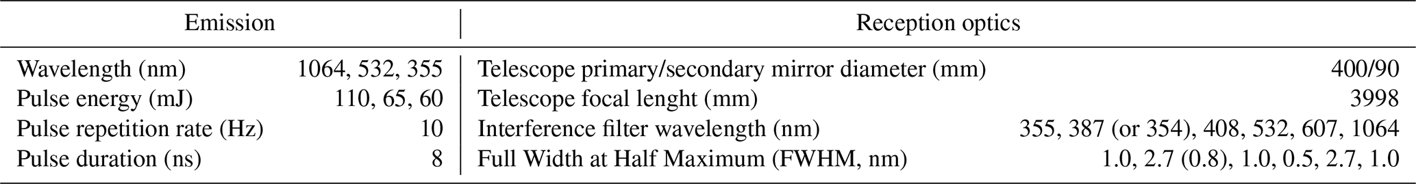
Lidar measurements were performed using the multi-wavelength Raman lidar (model LR331D400 Raymetrics S.A., Greece). A technical description of the main instrumental features is detailed in Table 1. The system is configured in a monostatic biaxial alignment pointing vertically to the zenith. A Nd:YAG laser emits pulses at 1064 nm (110 mJ), 532 nm (65 mJ) and 355 nm (60 mJ), with a repetition rate of 10 Hz and pulse duration of 8 ns. A 400 mm diameter Cassegrain telescope collects radiation due to scattering by atmospheric molecules and particles. The receiving subsystem also includes a wavelength separation unit with dichroic mirrors, interference filters, and a polarization cube. Detection is performed in seven channels: elastic wavelengths at 1064 nm, 532 nm (parallel and perpendicular polarisations), and 355 nm, as well as inelastic wavelengths at ∼607 nm (nitrogen Raman signal excited by 532 nm), ∼387 nm (nitrogen Raman signal excited by 532 nm radiation), and ∼408 nm (water vapour Raman signal excited by 355 nm). Since May 2017, the nitrogen Raman channel has been updated to 354 nm, serving as the molecular reference (nitrogen and oxygen). The instrument operates with a vertical resolution of 7.5 m. The system was incorporated into EARLINET in April 2005 and it is currently part of the ACTRIS research infrastructure (Laj et al., 2024), which has involved numerous instrument upgrades to fulfil ACTRIS requirements. In 2015, the dichroic mirror responsible for reflecting 355 nm and transmitting 532 and 1064 nm in the emitter system was replaced. In 2016, the optical path was checked, and the optimal tilt of the involved elements was adjusted. In December 2016, rotational Raman filters were implemented in the system to improve its capability for retrieving aerosol extinction at 355 nm (Veselovskii et al., 2015; Ortiz-Amezcua et al., 2020). As part of this update, the ∼387 nm interference filter was replaced by one centred at ∼354 nm. Until May 2017, the optical configuration to retrieve the water vapour mixing ratio used a vibrational-rotational (VR) nitrogen filter centred at ∼387 nm. Afterwards, the new configuration used the pure rotational (RR) Raman signal near 354 nm as the molecular reference. In both configurations, the water vapour Raman signal was measured with a VR filter at ∼408 nm. Consequently, all these modifications during the period 2009–2022 affected the overlap functions and the calibration constants to calculate the water vapour mixing ratio. More details about the system are provided in Díaz-Zurita et al. (2025).

Table 1 Technical details of the main optical elements of the Raman lidar system operated at the University of Granada.

2.3 Additional instrumentation

In this study, different reference instruments were used to calibrate lidar water vapour measurements, including in situ sensors such as radiosondes and remote sensing instruments like microwave radiometers and GNSS receivers. RS data were obtained using the GRAW DFM-09 RS (GRAW Radiosondes GmbH & Co., Germany), a lightweight radiosonde that provides measurements of temperature (resolution 0.01 °C, accuracy 0.2 °C), pressure (resolution 0.1 hPa, accuracy 0.3 hPa) and relative humidity (RH, resolution 1 %, accuracy better than 4 %) (Navas-Guzmán et al., 2014). Data acquisition and processing were carried out using the Grawmet software version 5.16 and a GS-E ground station from same RS manufacturer. This RS model has already been used as a reference measurement to retrieve water vapour content (e.g., Navas-Guzmán et al., 2014; Bedoya et al., 2017). In total, 148 radiosondes were launched during the period from 2009 to 2022. From them, only 31 radiosondes coincided with simultaneous nighttime Raman lidar measurements under clear sky conditions (clear skies being preferred for optimum radiosonde comparisons).

Microwave measurements were performed using the HATPRO microwave radiometer (RPG-HATPRO, Radiometer Physics GmbH), which has been operating at the UGR urban station since 2010. The MWR measures the sky brightness temperature continuously and automatically, with a precision of 0.3 and 0.4 K at a 1.0 s integration time. The radiometer uses direct detection receivers within two bands: 22–31 and 51–58 GHz. The first band provides information about the humidity profile of the troposphere and cloud liquid water content, while the second band contains information about the temperature profile due to homogeneous mixing of O₂ (Navas-Guzmán et al., 2016). Precipitable water vapour retrieval is obtained using a neural network approach with brightness temperature as the input, which provides a root mean square precision of ±0.2 kg m⁻² and a random uncertainty of 0.05 kg m⁻² for W product (https://www.radiometer-physics.de/, last access: 11 May 2026). Bedoya-Velásquez et al. (2019) analysed the MWR performance by comparison with RS measurements at the UGR urban station, finding that temperature and RH biases were lower under cloud-free conditions.

Ground-based GNSS stations were also used for W measurements, which are computed from the zenith total delay (ZTD) experienced by the signal travelling between the satellite and the ground receiver. ZTD is the sum of the zenith hydrostatic delay (ZHD) and zenith wet delay (ZWD), the latter being exclusively due to water vapour (Bevis et al., 1992). This can be converted into W using a multiplication factor, known as Davis temperature (Davis et al., 1985), that depends on the mean temperature of the atmosphere weighted by the water vapour profile. The processing of the GNSS data to produce ZTD values is carried out using Jet Propulsion Laboratory’s (JPL) GipsyX 1.0 software, which is fed with JPL’s Repro 3.0 orbits and clocks data, and Vienna Mapping Function 1 (Boehm et al., 2006) gridded data and mapping function parameters. JPL’s data and software can be obtained from https://gipsyx.jpl.nasa.gov/ (last access: 11 May 2026). All processing is performed by the Nevada Geodetic Laboratory (Blewitt et al., 2018). GNSS measurements have high temporal resolution (one measurement every 5 min), high accuracy (between 0.35 and 2 mm), and long-term stability (Schreiner et al., 2007; Teke et al., 2011). The selected station for our study is located at the Andalusian Institute of Geophysics (37.18° N, 3.59° W), approximately 2 km in a straight line from the UGR urban station.

2.4 Model data

Numerical Weather Prediction models are used to complement experimental measurements. In particular, this study uses ERA5, CAMS (Copernicus Atmosphere Monitoring Service) and MERRA2 (The Modern-Era Retrospective Analysis for Research and Applications, version 2) models. ERA5 is the fifth-generation European Centre for Medium-Range Weather Forecasts (ECMWF, Hersbach et al., 2020) reanalysis for global climate and weather. The data used have a spatial resolution of 0.25°×0.25°, with hourly temporal resolution, and 137 vertical levels (hybrid pressure/sigma). CAMS global reanalysis (EAC4, ECMWF Atmospheric Composition Reanalysis 4, Inness et al., 2019), which is the fourth version produced by ECMWF, provides data at 0.75°×0.75° spatial resolution, 3 h intervals and 60 vertical levels. Finally, MERRA2 (Gelaro et al., 2017) is the latest atmospheric reanalysis of the modern satellite era produced by NASA’s Global Modelling and Assimilation Office (GMAO) and offers data with a spatial resolution of 0.50°×0.625°, temporal intervals of 3 h, and 72 vertical model levels. The pressure and geopotential on model levels, as well as the geopotential height and geometric height, can be computed following the procedures described in the ECMWF documentation (https://confluence.ecmwf.int/display/CKB/ERA5%3A+data+documentation, last access: 11 May 2026).

3 Methodology

This section presents the water vapour Raman lidar technique, the retrieval of W and the calibration methods used to derive water vapour mixing ratio from Raman lidar measurements, based on water vapour profiles from RS data or W values from collocated reference instruments. Finally, a hybrid methodology is presented as a solution to the limitations of traditional radiosonde-based calibration methods.

3.1 Water vapour mixing ratio profiles from Raman lidar measurements

The water vapour Raman lidar technique uses the ratio of Raman scattering intensities from the water vapour molecule and a molecular reference, providing a direct measurement of the atmospheric water vapour mixing ratio (Whiteman et al., 1992, 2006). In this sense, the lidar equation can be expressed for the molecular reference and water vapour Raman signals as:

$$\begin{array}{}\text{(1)}& \begin{array}{rl}P(z,{\mathit{\lambda }}_i)& =P\left({\mathit{\lambda }}_{\mathrm{0}}\right)\cdot K_i\cdot {\displaystyle \frac{O_i\left(z\right)}{z^{\mathrm{2}}}}\\ & \cdot F_i\left[T\right(z\left)\right]N_i\left(z\right)\left[\mathrm{d}{\mathit{\sigma }}_i\right({\mathit{\lambda }}_{\mathrm{0}},\mathit{\pi })/\mathrm{d}\mathrm{\Omega }]\\ & \cdot \exp \left\{-\underset{\mathrm{0}}{\overset{z}{\int }}\left[\mathit{\alpha }\right(z^{\prime },{\mathit{\lambda }}_{\mathrm{0}})+\mathit{\alpha }(z^{\prime },{\mathit{\lambda }}_i\left)\right]\mathrm{d}{z}^{\prime }\right\}\end{array}\end{array}$$

where the sub-index i indicates the MR species or water vapour (H₂O); P(z,λ_i) is the backscattered signal from range z at the Raman shifted wavelengths; P(λ₀) is the emitted laser power at wavelength λ₀; ; O_i(z) is the overlap function; F_i[T(z)] is the temperature-dependent function of the Raman scattering (Whiteman, 2003; Whiteman et al., 2006), N_i(z) is the number density and $\mathrm{d}{\mathit{\sigma }}_i({\mathit{\lambda }}_{\mathrm{0}},\mathit{\pi })/\mathrm{d}\mathrm{\Omega }$ is the Raman backscatter cross section at the Raman shifted wavelength; α is the total extinction coefficient at wavelength λ₀, λ_MR, ${\mathit{\lambda }}_{{\mathrm{H}}_{\mathrm{2}}\mathrm{O}}$, respectively.

The water vapour mixing ratio is defined as the ratio of the mass of water vapour to the mass of dry air in a sample of the atmosphere (Goldsmith, 1998). Consequently, the ratio $N_{{\mathrm{H}}_{\mathrm{2}}\mathrm{O}}\left(z\right)/N_{\text{MR}}\left(z\right)$ is proportional to the water vapour mixing ratio (Whiteman et al., 1992, 2006). Assuming identical overlap factors and the range-independent Raman backscatter cross sections for the two signals, this ratio can be expressed as:

$$\begin{array}{}\text{(2)}& \begin{array}{rl}{\displaystyle \frac{N_{{\mathrm{H}}_{\mathrm{2}}\mathrm{O}}\left(z\right)}{N_{\text{MR}}\left(z\right)}}& ={\displaystyle \frac{P(z,{\mathit{\lambda }}_{{\mathrm{H}}_{\mathrm{2}}\mathrm{O}})}{P(z,{\mathit{\lambda }}_{\text{MR}})}}\cdot {\displaystyle \frac{F_{\text{MR}}\left[T\right(z\left)\right]}{F_{{\mathrm{H}}_{\mathrm{2}}\mathrm{O}}\left[T\right(z\left)\right]}}\cdot {\displaystyle \frac{K_{\text{MR}}{\mathit{\sigma }}_{\text{MR}}}{K_{{\mathrm{H}}_{\mathrm{2}}\mathrm{O}}{\mathit{\sigma }}_{{\mathrm{H}}_{\mathrm{2}}\mathrm{O}}}}\\ & \cdot \exp \left\{\underset{\mathrm{0}}{\overset{z}{\int }}\left[\mathit{\alpha }\right(z^{\prime },{\mathit{\lambda }}_{{\mathrm{H}}_{\mathrm{2}}\mathrm{O}})-\mathit{\alpha }(z^{\prime },{\mathit{\lambda }}_{\text{MR}}\left)\right]\mathrm{d}{z}^{\prime }\right\}\end{array}\end{array}$$

and thus,

$$\begin{array}{}\text{(3)}& \begin{array}{rl}r\left(z\right)& ={\displaystyle \frac{P(z,{\mathit{\lambda }}_{{\mathrm{H}}_{\mathrm{2}}\mathrm{O}})}{P(z,{\mathit{\lambda }}_{\text{MR}})}}\cdot {\displaystyle \frac{F_{\text{MR}}\left[T\right(z\left)\right]}{F_{{\mathrm{H}}_{\mathrm{2}}\mathrm{O}}\left[T\right(z\left)\right]}}\cdot K\\ & \cdot \exp \left\{\underset{\mathrm{0}}{\overset{z}{\int }}\left[\mathit{\alpha }\right(z^{\prime },{\mathit{\lambda }}_{{\mathrm{H}}_{\mathrm{2}}\mathrm{O}})-\mathit{\alpha }(z^{\prime },{\mathit{\lambda }}_{\text{MR}}\left)\right]\mathrm{d}{z}^{\prime }\right\}\end{array}\end{array}$$

where the term $P(z,{\mathit{\lambda }}_{{\mathrm{H}}_{\mathrm{2}}\mathrm{O}})/P(z,{\mathit{\lambda }}_{\text{MR}})$ represents the backscattered signal ratio, $F_{\text{MR}}\left[T\right(z\left)\right]/F_{{\mathrm{H}}_{\mathrm{2}}\mathrm{O}}\left[T\right(z\left)\right]$ is the ratio of the temperature-dependent functions for the Raman molecular reference and H₂O channels, and K is the calibration constant of the instrument that takes into account the fractional volume of nitrogen in the atmosphere (78.08 %), the ratio of the molecular masses, the range independent calibration constants K_MR and $K_{{\mathrm{H}}_{\mathrm{2}}\mathrm{O}}$, and the range-independent Raman backscatter cross sections σ_MR and ${\mathit{\sigma }}_{{\mathrm{H}}_{\mathrm{2}}\mathrm{O}}$. The determination of K using reference measurements and different methods is the cornerstone of this study. The assumption of identical overlap functions for molecular reference and H₂O might not be true in real applications and differences between both overlap functions are found in the near range (Whiteman et al., 2006).

The temperature dependence of RR and VR Raman scattering must also be considered. Whiteman (2003) assessed the required passbands for Raman scattering at various spectral widths using Nd:YAG excitation and determined the required filter passbands for water vapour measurements with minimal temperature sensitivity. According to this assessment, the filters used in the Raman lidar for water vapour (centred at ∼408 nm, FWHM=1 nm) and molecular reference (centred at ∼387 nm, FWHM=2.7 nm, or centred at ∼354 nm, FWHM=0.8 nm) select the Raman Stokes spectrum (∼387 nm) or Raman Anti-Stokes spectrum (∼354 nm), resulting in measurements essentially independent of temperature and making it reasonable to approximate the ratio $F_{\text{MR}}\left[T\right(z\left)\right]/F_{{\mathrm{H}}_{\mathrm{2}}\mathrm{O}}\left[T\right(z\left)\right]$ to 1.

The exponential term in Eq. (3) represents the difference in atmospheric transmission between the molecular reference and water vapour Raman wavelengths. In Díaz-Zurita et al. (2025), they evaluated this term at our station for two different optical configurations used to retrieve the water vapour mixing ratio: the first one using a VR nitrogen filter centred at ∼387 nm and the second one using a RR filter centred at ∼354 nm for the molecular reference. Both used a VR water vapour filter centred at ∼408 nm (Díaz-Zurita et al., 2025). The results demonstrated that this term should not be neglected for accurate water vapour lidar measurements and it ultimately depends on the aerosol load and its spectral dependence. Specifically, this term can deviate from the unit by up to 5.1 % at 6 km when using nitrogen at ∼387 nm, whereas with the RR Raman filter at ∼354 nm, the difference can reach up to 15 % at the same altitude. Under high aerosol load conditions, these deviations can increase by an additional 2 % and 6 %, respectively, relative to molecular conditions. This implies that neglecting the difference in atmospheric transmission would induce a systematic bias in the system. Conversely, when this term is calculated, the systematic bias is transformed into a random uncertainty (JCFG/GUM, 2020). To achieve this, we first calculate the molecular contribution using Rayleigh scattering based on temperature T(z) and pressure P(z) profiles (Bucholtz, 1995; Mattis et al., 2002) from ECMWF model data for Granada (O'Connor, 2025), available from the ACTRIS Data Centre (https://hdl.handle.net/21.12132/1.16d392060df54287, last access: 11 May 2026). The aerosol contribution is then estimated from sun photometer aerosol optical depth (AOD) values, modelling the vertical distribution of aerosol extinction using an exponential decay function with altitude (Díaz-Zurita et al., 2025). Both contributions allowed the estimation of the differential atmospheric transmission term, enabling its systematic calculations across the water vapour mixing ratio dataset.

3.2 Precipitable water vapour

Precipitable water vapour is defined as the total atmospheric water vapour contained in a vertical column of unit cross section, extending in terms of the height to which that water substance would stand if completely condensed and collected in a vessel of the same unit cross section (American Meteorological Society, 2014). Its units are expressed in terms of length (cm or mm), which are equivalent to surface concentration units (g cm⁻² or kg m⁻²) when assuming the density of liquid water in 1 g cm⁻³ (Vaquero-Martínez et al., 2019). Mathematically, W can be obtained as the integration along the vertical path of the water vapour density ${\mathit{\rho }}_{{\mathrm{H}}_{\mathrm{2}}\mathrm{O}}\left(z\right)$ as a function of height.

$$\begin{array}{}\text{(4)}& W=\underset{\mathrm{0}}{\overset{z}{\int }}{\mathit{\rho }}_{{\mathrm{H}}_{\mathrm{2}}\mathrm{O}}\left(z^{\prime }\right)d{z}^{\prime }\end{array}$$

The computation of ${\mathit{\rho }}_{{\mathrm{H}}_{\mathrm{2}}\mathrm{O}}\left(z\right)$ can be done from Raman lidar r(z) and dry air density ρ_air(z) profiles as:

$$\begin{array}{}\text{(5)}& {\mathit{\rho }}_{{\mathrm{H}}_{\mathrm{2}}\mathrm{O}}\left(z\right)=r\left(z\right)\cdot {\mathit{\rho }}_{\text{air}}\left(z\right)\end{array}$$

where, ρ_air(z) can be calculated from pressure and temperature profiles as (Dai et al., 2018):

$$\begin{array}{}\text{(6)}& \begin{array}{rl}& {\mathit{\rho }}_{\text{air}}\left(z\right)=\mathrm{348.328}\cdot {\displaystyle \frac{P\left(z\right)}{T\left(z\right)}}\\ & \cdot \left[\mathrm{1}+P\left(z\right)\left(\mathrm{57.9}\times {\mathrm{10}}^{-\mathrm{8}}-{\displaystyle \frac{\mathrm{0.94581}\times {\mathrm{10}}^{-\mathrm{3}}}{T\left(z\right)}}+{\displaystyle \frac{\mathrm{0.25844}}{T(z{)}^{\mathrm{2}}}}\right)\right]\end{array}\end{array}$$

The first limitation in the computation of W using Raman lidar measurements is the incomplete overlap region, which is typically the region with the highest water vapour content. This limitation requires the use of assumptions in the incomplete overlap region, which are detailed in the following section. Another limitation is the need to exclude noisy regions or cases where lidar measurements do not adequately represent the entire atmospheric profile. To address this, the W calculation is performed only within the height range where the SNR of the lidar water vapour mixing ratio profile is greater than 0.3. If the upper limit of this range is less than 5 km above ground level (km a.g.l.), the W value is not computed. The 0.3 threshold was determined to ensure data quality as proposed by Miri et al. (2024). Additionally, lidar W values were evaluated against RS W values to verify their quality.

3.3 Calibration methods from Raman lidar water vapour observations

3.3.1 Traditional radiosonde-based calibration methods

The first calibration method used in this research is the traditional radiosonde calibration, which is based on simultaneous and collocated RS and lidar measurements. In particular, two different approaches for this method were evaluated, from which the calibration constant K₁ was determined. The first approach is the profile method (Whiteman et al., 1992; Mattis et al., 2002; Reichardt et al., 2012), which estimates the calibration constant K_i as the mean ratio between the water vapour mixing ratio from RS and the uncalibrated lidar profile ($r_{\text{lidar}}^{\prime }$) within a selected height range (z₁, z₂):

$$\begin{array}{}\text{(7)}& K_i={\displaystyle \frac{\mathrm{1}}{N}}\sum _{m=z_{\mathrm{1}}}^{z_{\mathrm{2}}}{\displaystyle \frac{r_{\text{RS}}\left(z_m\right)}{r_{\text{lidar}}^{\prime }\left(z_m\right)}}\end{array}$$

where z₁ and z₂ represent the lower and upper limits of the selected height range, respectively, and N is the total number of data points within this range.

The second approach is the iterative method, which determines the calibration constant K_j through an iterative least squares fitting within the selected height range. The approach is optimised by removing points that deviate from the regression line by more than one standard deviation (SD). The remaining points are used again to perform a new least squares regression. This process is repeated until the slope of the linear regression changes by less than 1 %. If the number of remaining points is less than 50 % of the initial number, the calibration is considered invalid. The slope of the linear regression is taken as the value of K_j (Navas-Guzmán et al., 2014).

In both approaches, different height ranges are analysed within the 1.0–4.5 km interval (e.g., 1.0–4.5, 2.0–4.5, 2.5–4.0, and 3.0–4.5 km). The chosen layers corresponded to regions with a high water vapour mixing ratio. The upper limit for the lidar was set at 4.5 $\mathrm{km}\mathrm{a}.\mathrm{g}.\mathrm{l}.$ to ensure a sufficiently high SNR in the lidar measurements and to minimise the effects of sonde drift with altitude due to winds. Once both approaches are evaluated, the final calibration constants K₁ is selected between K_i and K_j as the one that best fits the lidar water vapour mixing ratio profile to that of the RS. It is evaluated using several fitting parameters, including the slope, intercept, and coefficient of determination (R²), as well as statistical metrics such as mean bias, SD, and root mean square error (RMSE).

3.3.2 Integrated column calibration method

The second calibration method is the well-known integrated column method, which is based on W measurements from a collocated reference instrument (Dai et al., 2018). The calibration constant, K₂, is computed as:

$$\begin{array}{}\text{(8)}& K_{\mathrm{2}}={\displaystyle \frac{W_{\text{ref}}}{W_{\text{lidar}}^{\prime }}}\end{array}$$

where W_ref is the W value from a reference instrument, and $W_{\text{lidar}}^{\prime }$ is the integrated value from the uncalibrated lidar profile.

The advantage of this method is the use of existing reference instruments, which provide a high availability of water vapour observations, resulting in the determination of the calibration constant with higher temporal resolution. However, the incomplete overlap in lidar measurements presents a disadvantage for this calibration method, as assumptions must be made about water vapour measurements in that region. In our computations, K₂ is determined by assuming constant uncalibrated lidar values from the ground to the first point where complete overlap is achieved. The altitude of complete overlap was determined by comparing the lidar water vapour mixing ratio with collocated radiosonde profiles, identifying the point at which the profiles show consistent behaviour.

3.3.3 Hybrid calibration method

The third method proposed in this study is the hybrid methodology, which aims to address the limitations caused by the low number of correlated RS profiles and the issues related to the incomplete overlap region inherent to lidar systems. The hybrid method employs correlative W observations from a reference instrument (e.g., GNSS or MWR) with higher data availability than other sources, thereby increasing the number of calibration cases. This method also corrects and optimises the uncalibrated lidar profile in the incomplete overlap region by fitting the water vapour mixing ratio shape in this region to that provided by the NWP model (Sect. 2.4). Consequently, the new uncalibrated lidar profile ($r_{\text{lidar}}^{\prime \prime }$) is a combination of the model derived shape in the incomplete lidar overlap region and the uncalibrated lidar profile above this zone, obtained as follows:

$$\begin{array}{}\text{(9)}& r_{\text{lidar}}^{\prime \prime }\left(z\right)=\left\{\begin{array}{ll}{r}_{\text{model}}^{\prime }\left(z\right),& \text{for }\mathrm{0}\le z\le z_{\text{overlap}}\\ r_{\text{lidar}}^{\prime }\left(z\right),& \text{for }{z}_{\text{overlap}}<z\le z_n\end{array}\right.\end{array}$$

where $r_{\text{model}}^{\prime }(\mathrm{0},z_{\text{overlap}})$ represents the profile shape from the reanalysis model, which was used to scale the uncalibrated lidar profile in the incomplete overlap region. To do so, the model's profile is forced to match the first uncalibrated lidar value measured in the complete overlap region. The uncalibrated lidar profile above this zone is $r_{\text{lidar}}^{\prime }(z_{\text{overlap}},z_n)$, where z_overlap represents the height at which complete overlap is achieved, and z_n is the upper limit defined up to the first height where the SNR of the lidar profile is less than 0.30. A validation of this method is presented in Sect. 4.3.

The calibration constant (K₃) for the new uncalibrated lidar profile is determined as follows:

$$\begin{array}{}\text{(10)}& K_{\mathrm{3}}={\displaystyle \frac{W_{\text{ref}}}{W_{\text{lidar}}^{\prime \prime }}}\end{array}$$

where $W_{\text{Lidar}}^{\prime \prime }$ is the integrated value from the new uncalibrated lidar profile.

Thus the hybrid calibration method relies on the accurate computation of W from lidar measurements, it is essential that the lidar measurements adequately represent the entire atmospheric profile used for W integration. While clear-sky conditions are preferred mainly to avoid limitations associated with noisy profiles during vertical integration, the methodology can also be applied under partly cloudy conditions, if the cloud base is located above the altitude range used for W integration and if the lidar SNR remains sufficiently high (greater than 0.3). Its applicability in the presence of low clouds depends on the size, frequency, and distribution of cloud-free gaps. Provided these gaps are sufficiently large and frequent, the lidar can acquire measurements with adequate SNR, enabling reliable vertical integration and temporal averaging. It should be noted that the achievable SNR depends strongly on specific system characteristics, such as laser power, optical configuration, and detector performance. Therefore, the hybrid methodology can be applied under partly cloudy conditions but depends explicitly on these system characteristics.

Once the lidar system is calibrated, the hybrid methodology does not use lidar measurements in the incomplete overlap region. Indeed, it assumes that the water vapour mixing ratio profile follows the profile described by a reanalysis model in the complete overlap region down to the ground. This method, which estimates the lidar water vapour mixing ratio profile in the lower troposphere, enables reliable measurements and provides the vertical distribution of water vapour in these layers without assuming any predefined shape (e.g., constant, exponential decay).

4 Results and discussion

This section provides a detailed analysis of the calibration methods applied to retrieve water vapour from Raman lidar measurements. The evaluation includes comparisons of lidar-derived water vapour mixing ratio profiles for each calibration method with RS data. The methodology also enables the generation of a high temporal resolution dataset of lidar calibration constants. Furthermore, this section explores the temporal and vertical variability of water vapour, emphasizing its importance in atmospheric studies.

4.1 Radiosonde-based calibration of Raman lidar water vapour mixing ratio profiles

Water vapour mixing ratio values were retrieved from Raman lidar data for the period 2009–2022 using traditional (Sect. 3.3.1) and integrated column (Sect. 3.3.2) calibration methods, both based on RS measurements. Only nighttime data were used to avoid the high background noise from daylight. The temporal resolution of the lidar profiles was 30 min, coinciding with radiosonde launches, whose profiles were interpolated to match the lidar vertical resolution of 7.5 m.

It should be noted that, due to the different upgrades of the lidar system, there were changes in the region affected by incomplete overlap. During the first period, before May 2017, the overlap zone extended up to 700 $\mathrm{m}\mathrm{a}.\mathrm{g}.\mathrm{l}.$ (Fig. 1c). Following significant adjustments to the system’s optical configuration, the incomplete overlap region was reduced to 300 $\mathrm{m}\mathrm{a}.\mathrm{g}.\mathrm{l}.$ during the second period (from June 2017 onwards) (Fig. 1h). Considering the 31 simultaneous RS launches made alongside lidar measurements, this region accounted for 29 % ± 5 % and 11 % ± 2 % of the total lidar W during the first and second periods, respectively.

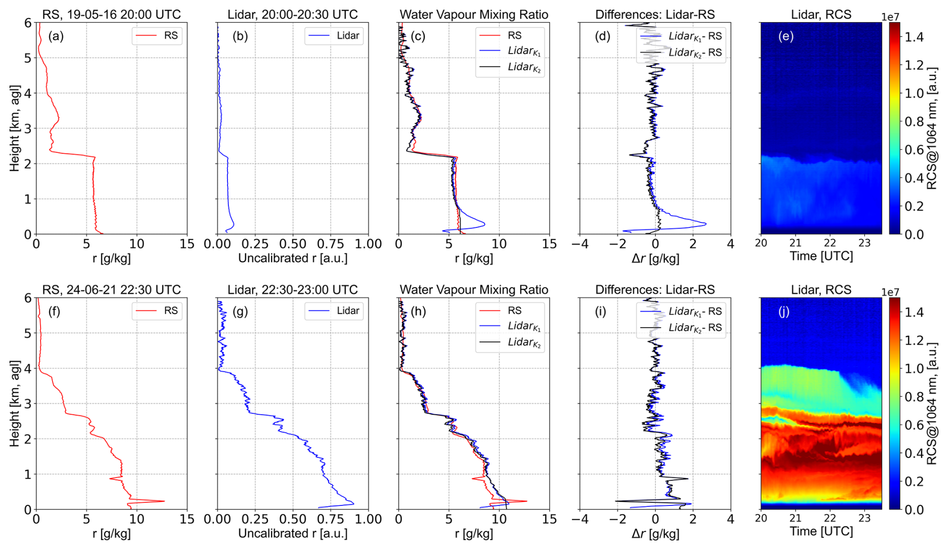
Figure 1 (a) Radiosonde water vapour mixing ratio profile. (b) Uncalibrated lidar profile. (c) RS and calibrated lidar water vapour mixing ratio profiles. (d) Differences between calibrated lidar and RS profiles. (e) Temporal evolution of vertical profiles of RCS at 1064 nm. The upper panels correspond to 19 May 2016, and the lower panels show the same information for 24 June 2021.

Figure 1 presents two different cases that were studied to evaluate the performance of the traditional methods based on correlative RS and precipitable water vapour measurements. The days selected were 19 May 2016 (Case I, upper panels) and 24 June 2021 (Case II, lower panels). Table 2 shows the calibration constants (K₁ and K₂) for these two nights, including also the linear fit parameters and statistics of the differences in water vapour mixing ratio between lidar and RS. In both case studies, the differences observed between Raman lidar and RS above the incomplete lidar overlap region are very small and may be attributed to radiosonde drift caused by the wind and to the noise in the lidar signal at higher altitudes (Brocard et al., 2013; Foth et al., 2015; Dai et al., 2018).

Table 2 Linear fit parameters (slope, intercept, and R²) and statistics of the differences in water vapour mixing ratio between lidar and radiosondes. The incomplete overlap region was excluded from the calculation. Calibration constants were obtained using traditional (K₁, Sect. 3.3.1) and integrated column (K₂, Sect. 3.3.2) methods, both based on RS measurements.

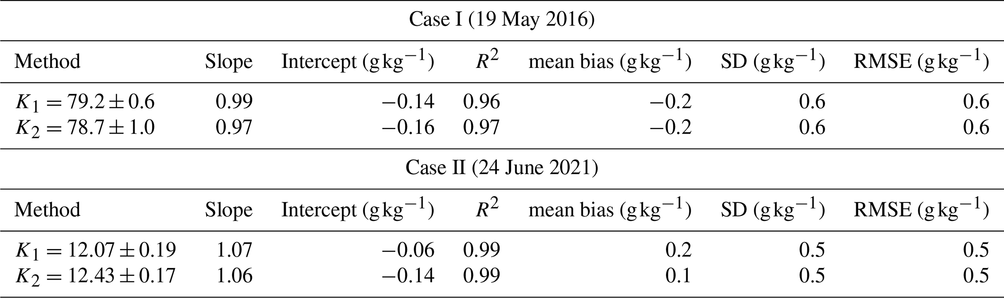
For Case I (Fig. 1, upper panels), the temporal evolution of the lidar Range Corrected Signal (RCS) at 1064 nm between 20:00 and 23:30 UTC (Fig. 1e) reveals the presence of an aerosol layer extending up to 2.3 $\mathrm{km}\mathrm{a}.\mathrm{g}.\mathrm{l}.$ Within this layer, the RCS at 1064 nm, RS water vapour mixing ratio profile (panel a), and the uncalibrated lidar profile (panel b) were almost constant with height, suggesting homogeneity and stability in the lower troposphere with a well-mixed layer during this period (Granados-Muñoz et al., 2015; Navas-Guzmán et al., 2019). Figure 1c displays the RS (red curve) and the calibrated lidar water vapour mixing ratio profiles obtained using the first and second calibration methods (blue and black curves, respectively), for the period from 20:00 to 20:30 UTC. As discussed in Sect. 3.3, the traditional method based on RS determines the calibration constants for different height ranges, the final value of K₁ being the best fit between lidar and RS profiles. For this particular case, the selected range was 1–2 $\mathrm{km}\mathrm{a}.\mathrm{g}.\mathrm{l}.$, resulting in a K₁ value of 79.2 ± 0.6 g kg⁻¹. On the other hand, with the correlative W measurements (black curve), the K₂ value obtained was 78.7 ± 1.0 g kg⁻¹. The difference between K values was negligible (below 1 % and within the uncertainty ranges), suggesting that assuming constant water vapour values in the incomplete overlap region can be a good approximation in the presence of well-mixed layers, such as the one observed that night (Granados-Muñoz et al., 2015; Navas-Guzmán et al., 2019).

The differences between lidar and RS are illustrated in Fig. 1d. A good agreement between the calibrated lidar water vapour mixing ratio profiles retrieved using the different methods and the RS profile was obtained above the incomplete overlap region, with a mean bias and SD of −0.2 ± 0.6 g kg⁻¹ (Table 2) for both methods. However, below this zone, the differences were larger for the RS calibration method (blue line), with a mean bias of 1.0 ± 1.3 g kg⁻¹; therefore, lidar data in the incomplete overlap region are clearly unreliable (Fig. 1d), and must be corrected. For data using the integrated column method, which assumes constant water vapour values in the incomplete overlap region, the differences are very small (0.14 ± 0.14 g kg⁻¹), as expected, since it assumes a reasonably constant behaviour in the incomplete lidar overlap region. Results from Table 2 also demonstrate a good agreement between both profiles, with a linear correlation coefficient of 0.96 and 0.97, a slope close to one, and a low intercept (−0.16 g kg⁻¹).

Case II (Fig. 1, lower panels) is representative of a situation with a more heterogeneous aerosol distribution in the vertical range, characterised by the presence of decoupled layers (Fig. 1j). RS water vapour mixing ratio and uncalibrated lidar profiles are shown in Fig. 1f and g, respectively, for the period from 22:30 to 23:00 UTC. Radiosonde data reveal two very distinct structures of water vapour mixing ratio, showing a constant decrease from surface values of 10 g kg⁻¹ to approximately 6.8 g kg⁻¹ at 2 $\mathrm{km}\mathrm{a}.\mathrm{g}.\mathrm{l}.$ Above 2 $\mathrm{km}\mathrm{a}.\mathrm{g}.\mathrm{l}.$, water vapour continues decreasing with values of 3.4 g kg⁻¹ at 2.7 km where the decoupled layer appeared. Figure 1h displays the water vapour mixing ratio profiles obtained by RS and lidar, while the differences (lidar-RS) are shown in Fig. 1i. The values of the calibration constants were K₁=12.07 ± 0.19 g kg⁻¹ (calibration ranges: 1.0 to 4.5 $\mathrm{km}\mathrm{a}.\mathrm{g}.\mathrm{l}.$) and K₂=12.43 ± 0.17 g kg⁻¹. The difference between the K values for this case (3 %) was greater than that observed in Case I (which were below 1 %, Fig. 1, upper panels), suggesting that the assumption of constant water vapour values for the incomplete overlap region (first 300 $\mathrm{m}\mathrm{a}.\mathrm{g}.\mathrm{l}.$) is less appropriate. Overall, there was a good agreement between lidar and RS using both calibration methods, with the only notable difference observed in the incomplete overlap region (Fig. 1i). The linear fit parameters and statistical metrics between lidar and RS (Table 2) confirmed the good performance of water vapour measurements above this zone, with a higher determination coefficient (0.99) and a low intercept (−0.14 g kg⁻¹), as well as a mean bias and SD of 0.2 ± 0.5 and 0.1 ± 0.5 g kg⁻¹ for the traditional RS calibration and integrated column methods, respectively.

Figure 2a shows the temporal evolution of K values obtained using the first and second calibration methods for the period 2009–2022, based on 31 simultaneous RS and lidar measurements. The main outcome is that the calibration constants exhibited significant temporal variability, with values ranging from approximately 200 g kg⁻¹ in 2011 to 10 g kg⁻¹ in 2022. The maximum K value was 198 ± 5 g kg⁻¹ on 28 July 2011, which agrees with the previous study by Navas-Guzmán et al. (2014). The minimum K value was 10.5 ± 0.1 g kg⁻¹ on 26 May 2020. The significant differences in K between 2014 and 2017 can be explained by the modifications made in the Raman lidar optical configuration (see Sect. 2.2). Similar variabilities in the calibration constants when changing system design have also been reported for other systems in the EARLINET network (e.g., Stachlewska et al., 2017).

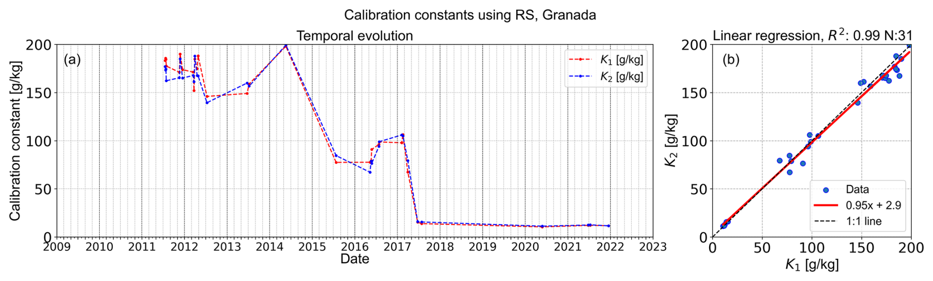
Figure 2 (a) Temporal evolution of K values using RS data. (b) Scatter plot of K values from the integrated column (y axis) and traditional RS (x axis) calibration methods. The red line represents the regression line, while the dashed black line represents the identity line.

The differences in calibration between the two methods based on correlative RS measurements, K₂ and K₁, were evaluated for the two identified periods. In the first period (up to May 2017, Fig. 2a), the mean bias was −3 ± 8 g kg⁻¹, with the largest discrepancies between 2011 and 2014 (mean bias of −5 ± 8 g kg⁻¹). These differences could be associated with the larger incomplete overlap region of the system (Navas-Guzmán et al., 2011), as well as the assumption of constant water vapour values in this region, leading to a relative difference of −1 % ± 7 % compared to RS W for this period. In the second period (after June 2017, Fig. 2a), the differences between K values were smaller than in the first period, with a mean bias of 0.6 ± 0.5 g kg⁻¹, likely due to improved system optimisation that resulted in a smaller overlap region (around 300 $\mathrm{m}\mathrm{a}.\mathrm{g}.\mathrm{l}.$). Figure 2b presents a direct inter-comparison of K₂ versus K₁. The 1:1 line and the linear fit are also plotted. A strong agreement between the two calibration constants was observed, with a high correlation (R²=0.99) and data closely aligned to the 1:1 line, exhibiting a slope of 0.95. The intercept (2.9 g kg⁻¹) suggests that assuming constant water vapour values in the incomplete overlap region may not always be appropriate. Due to the high variability (SD=45 g kg⁻¹) and the limited number of K values available (only 31) during the study period (2009–2022), this dataset may be insufficient to evaluate how changes in the setup of the Raman lidar system with time affected its capability to retrieve high-accuracy water vapour mixing ratio profiles.

4.2 Hybrid calibration method for Raman lidar water vapour mixing ratio profiles

The hybrid methodology introduced in Sect. 3.3.3 addresses the limitations of the traditional RS-based methods discussed in Sect. 4.1. First, it is necessary to study the optimal W database at the AGORA station. To achieve this, the W values obtained from remote sensing measurements (GNSS and MWR) and from reanalysis models (ERA5, CAMS, and MERRA2) were evaluated against those retrieved by radiosondes. For this study, the availability of RS data was not limited to those correlated with lidar observations, allowing the analysis of a larger database that includes 73 simultaneous RS launches with corresponding W measurements. To ensure data quality, outliers and incorrect data were removed by applying quality control filters. MWR data were excluded during precipitation, and GNSS W data with uncertainties exceeding 5 % were omitted. Figure 3 shows these different W measurements and values from models versus radiosonde data. The plots also contain the 1:1 line with the ordered pairs (W_RS, W_i), where i stands for the various other W sources (GNSS, MWR, ERA5, CAMS, and MERRA2), along with the linear fits. The parameters of the linear fits, as well as other statistical parameters, are summarised in Table 3.

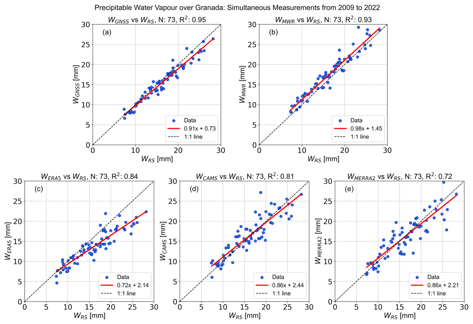
Figure 3 Precipitable water vapour scatter plots of GNSS, MWR, ERA5, CAMS, and MERRA2 (y axis, panels a–e, respectively) versus RS (x axis). The red lines represent the regression lines, and the dashed black lines represent the identity line.

Table 3 Linear fit parameters (slope, intercept and R²) between W from various sources and RS. The table also includes statistics of the differences of precipitable water vapour from different datasets and RS.

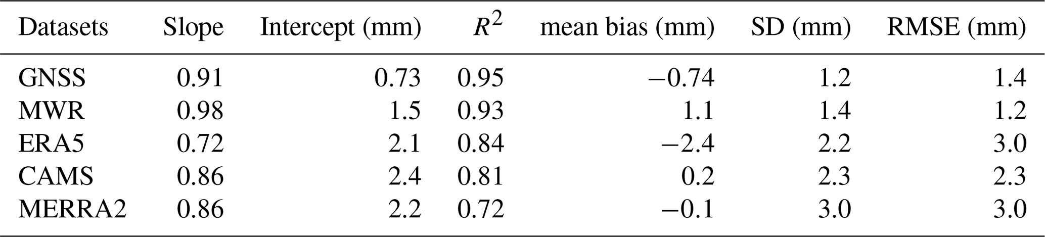
Results from Fig. 3 and Table 3 show very good agreement in W between measurements by remote sensing instrumentation and RS (top panels), with an excellent correlation (R²≥0.93) and slopes close to one (0.91 for GNSS and 0.98 for MWR). The negative bias (−0.74 mm) observed for GNSS suggests that GNSS slightly underestimates the RS values. This underestimation of W (by approximately 4 %) appears to be dependent on W values, becoming pronounced at higher W values (Fig. 3a). These results are in agreement with other studies (e.g., Schneider et al., 2010; Bock et al., 2016; Vaquero-Martínez et al., 2019; Huang et al., 2021; Paz et al., 2023). On the other hand, MWR slightly overestimated W by approximately 8 %, which is in agreement with the literature (e.g., Foth et al., 2015; Fragkos et al., 2019; Vaquero-Martínez et al., 2023). This bias appears rather independent of W value (Fig. 3b). This can be considered as a very good result because typical uncertainties in W estimations by MWR are around 10 % (Foth et al., 2015). Overall, the statistical analysis of the differences (Table 3) revealed that the best agreements versus RS are found for GNSS (mean bias and SD of −0.74 ± 1.2 mm, RMSE of 1.4 mm), and therefore GNSS data are selected as the most appropriate data to be used in the hybrid methodology.

Evaluations of model data versus RS also reveal good agreements (Fig. 3, lower panels), although with greater dispersion compared to GNSS and MWR. The bias in the models also exhibits a dependence on W values. In fact, in Table 3, the largest differences and the lowest correlations were obtained for W model values. There are some important points to make when assessing the comparisons of each model with RS. ERA5 had the smallest SD (2.2 mm) compared to CAMS and MERRA2 (2.3 and 3 mm), and achieved a higher R² value (0.84 versus 0.81 and 0.72, respectively). However, the RMSE was higher for ERA5 than for the CAMS model.

Since model data are available for the entire study period, the complete RS database from the AGORA station was used, including 148 launches between 2009 and 2022. In addition, the models provide vertical information on the distribution of water vapour mixing ratio, which can be evaluated against RS observations. Figure 4a illustrates an example that demonstrates the improved capability of the models to reproduce the water vapour mixing ratio patterns within the incomplete overlap region. Lidar profiles are also shown. This case corresponds to 25 July 2011 at 20:41 UTC, when a radiosonde was launched at the UGR station, and clearly shows that the models reproduce the RS profile behaviour in the incomplete overlap region more accurately. This is supported by the statistical analysis of the differences in water vapour mixing ratio profiles between models and RS, as shown in Table 4 and Fig. 4b–d.

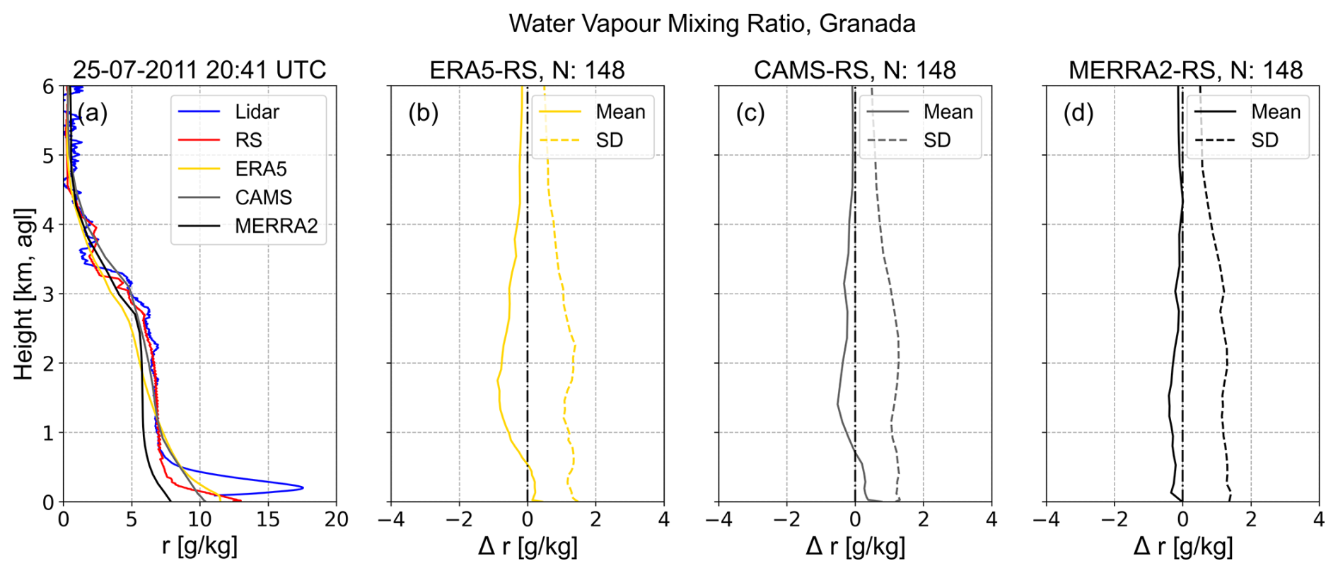
Figure 4 (a) Water vapour mixing ratio profiles from Raman lidar (blue), RS (red), ERA5 (gold), CAMS (gray), and MERRA2 (black) on 25 July 2011 at 20:41 UTC. Differences between models and RS data for ERA5 (b), CAMS (c), and MERRA2 (d). Solid curves represent the mean bias, while dashed curves indicate the standard deviation.

Table 4 Statistics of the differences in the water vapour mixing ratio between lidar and RS measurements, as well as between models and RS data, within the first 700 $\mathrm{m}\mathrm{a}.\mathrm{g}.\mathrm{l}.$ Mean bias and SD are expressed as mean values ± standard deviation for the height range.

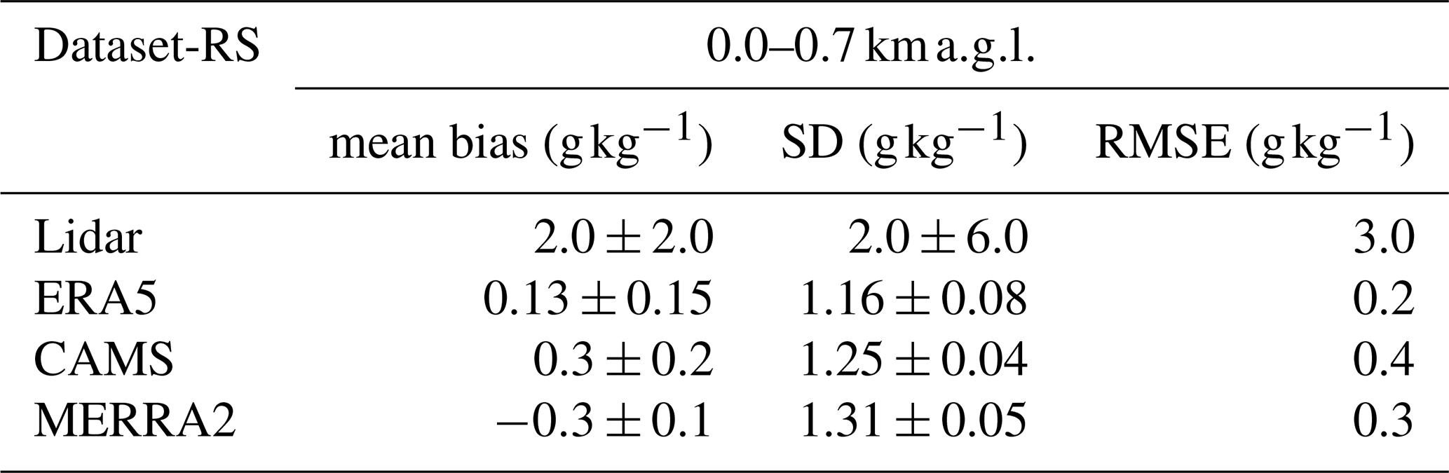
A detailed analysis of these differences for the 148 RS launches is presented in Fig. 4b–d, including both day and night data, and across a wide range of meteorological conditions. Solid curves represent the mean bias, while dashed curves show the standard deviations of the differences. Table 4 summarises the main statistical parameters (mean bias, SD, RMSE) for the incomplete overlap region (below 700 $\mathrm{m}\mathrm{a}.\mathrm{g}.\mathrm{l}.$). Only the statistics of the differences within the first 700 m are presented, as this represents the maximum incomplete overlap region encountered by our Raman lidar system.

Table 4 clearly shows that within the incomplete overlap region, the differences in water vapour mixing ratio profiles between NWP models and radiosondes are smaller (e.g., RMSE less than 0.4 g kg⁻¹), demonstrating a clear improvement over lidar measurements in that region, which exhibited a RMSE of 3 g kg⁻¹. More specifically, ERA5 (Fig. 4b) presented the best agreements, with the lowest mean bias (0.13 ± 0.15 g kg⁻¹), SD (1.16 ± 0.08 g kg⁻¹), and RMSE (0.2 g kg⁻¹). Also, from Fig. 4b and c, it can be observed that both ERA5 and CAMS overestimate the RS values below 700 $\mathrm{m}\mathrm{a}.\mathrm{g}.\mathrm{l}.$, while MERRA2 (Fig. 4d) showed a slight underestimation. At greater heights, NWP models generally underestimated RS values, likely because the models become less reliable, which can be attributed to greater uncertainty associated with the lower concentration of water vapour (Noh et al., 2016). Additionally, warm biases in temperature at higher altitudes may also contribute to these discrepancies (Noh et al., 2016). Nevertheless, NWP data above the incomplete overlap region are not critical for the hybrid calibration methodology. Finally, although the differences among the models were not statistically significant (Table 4), the ERA5 model was selected for the hybrid methodology due to its higher temporal and spatial resolution. This is consistent with the study by Huang et al. (2021), who indicated that ERA5 outperformed MERRA2 at most RS stations, largely due to its higher spatial resolution.

Based on the preceding analysis, the hybrid methodology uses GNSS-derived W as a reference for water vapour content and combines the uncalibrated lidar profile with the ERA5 model shape in the lower part to correct the incomplete overlap region. This method provides a reliable solution to the temporal limitations of traditional RS-based calibration methods and provides the vertical distribution of water vapour within the incomplete lidar overlap region. In contrast, the integrated column method presented previously assumed that water vapour mixing ratio in the incomplete overlap region is constant and equal to the first data point in the complete overlap region. To compare the hybrid methodology and the integrated column method, Fig. 5 presents several examples of water vapour mixing ratio profiles from Raman lidar measurements using both methods, along RS profiles. The four examples correspond to 25 July 2011 (20:41–21:11 UTC), 19 May 2016 (20:00–20:30 UTC), 25 July 2016 (20:09–20:39 UTC), and 26 May 2020 (21:33–22:03 UTC) (panels a to d). Insets within each panel provide a zoom of the water vapour mixing ratio profiles within the first km a.g.l.

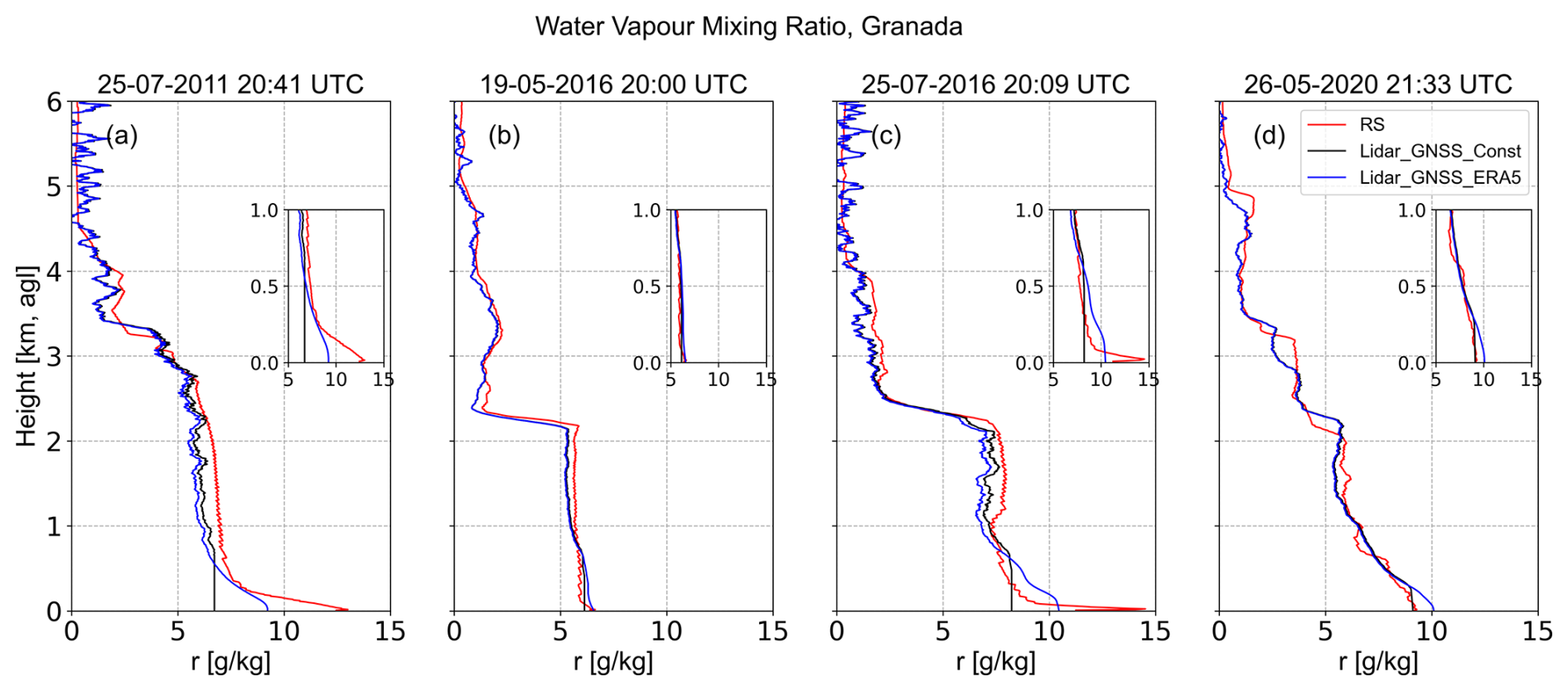
Figure 5 Calibrated lidar water vapour mixing ratio profiles using the integrated column and hybrid methods for 25 July 2011, 19 May 2016, 25 July 2016, and 26 May 2020 (panels a–d, respectively). The red curves represent RS profiles, while the black and blue curves show lidar profiles assuming constant values and the shape of the model in the incomplete lidar overlap region, respectively.

Results from Fig. 5 reveal very good agreement in water vapour mixing ratio between both methodologies and RS (red curves) in regions with complete overlap, with SDs ranging from 0.6–1.3 and 0.5–1.2 g kg⁻¹ for the integrated column (black curves) and hybrid methods (blue curves), respectively. The minimum SD was observed on 19 May 2016, while the maximum SD occurred on 25 July 2016. However, even though there are still good agreements, some remarkable peculiarities are observed in the incomplete overlap region. In particular, when the Atmospheric Boundary Layer (ABL) was well-mixed (e.g., 19 May 2016, Fig. 5b), lidar water vapour mixing ratio profiles obtained with both calibration methods can be considered adequate. In this case, the K values obtained with the integrated column method (K₂=78.7 ± 1.6 g kg⁻¹) or the hybrid methodology (K₃=77.9 ± 1.6 g kg⁻¹) showed no significant differences (0.8 g kg⁻¹). However, remarkable differences were observed when the conditions were not well-mixed (panels a, c, and d). The profiles obtained with the hybrid methodology show the best agreement, yielding SDs of 0.9, 1.0, and 0.4 g kg⁻¹, compared to SDs of 1.7, 1.4, and 0.3 g kg⁻¹ when assuming constant water vapour values in the incomplete overlap region. In these cases, significant differences were observed between the K values, with values of K₂=172 ± 3 g kg⁻¹ and K₃=164 ± 2.4 g kg⁻¹ on 25 July 2011, and K₂=93.5 ± 1.7 g kg⁻¹ and K₃=88.7 ± 1.6 g kg⁻¹ on 25 July 2016. These examples demonstrate that a good estimation of the vertical distribution of water vapour in the lower regions can be obtained with the hybrid method under both stable and unstable conditions. In addition, it should be noted that assuming constant values for water vapour is not always an appropriate approximation.

4.3 Evaluation of water vapour mixing ratio profiles with Raman lidar versus radiosonde measurements

A validation of water vapour mixing ratio profiles with the calibrated Raman lidar system versus RS was carried out. Again, there were only 31 correlative RS with lidar during nighttime clear-sky conditions, which are typically associated with more stable atmospheric conditions. Figure 6 illustrates the differences between water vapour mixing ratio obtained with lidar and RS, showing the analyses for the whole period (2009–2022) and also differentiating between the first (until May 2017) and second (from June 2017 onwards) periods, which facilitates an assessment of the impact of the different ranges of the incomplete overlap region. Table 5 provides statistics of differences for different height ranges: the entire profile (0–6 $\mathrm{km}\mathrm{a}.\mathrm{g}.\mathrm{l}.$), the maximum incomplete overlap region (0–0.7 $\mathrm{km}\mathrm{a}.\mathrm{g}.\mathrm{l}.$), and the region above 0.7 $\mathrm{km}\mathrm{a}.\mathrm{g}.\mathrm{l}.$

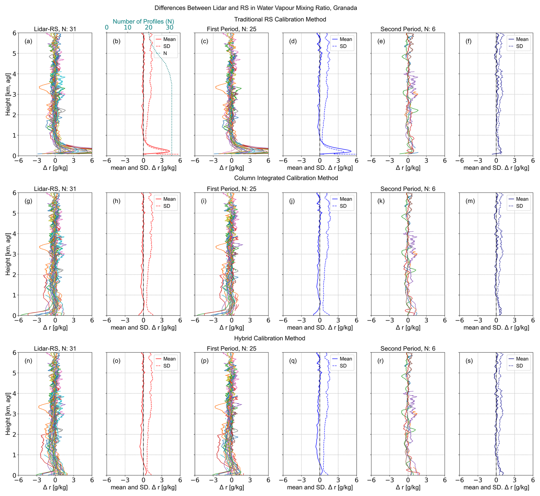
Figure 6 Nighttime differences between Raman lidar and RS water vapour mixing ratio profiles, using calibration constants from the traditional RS (K₁), integrated column (K₂) and hybrid (K₃) methods (upper, middle and lower panels, respectively). Panels (a), (b), (g), (h), (n), and (o) show the differences for the entire period, while panels (c), (d), (i), (j), (p), and (q) display results for the first period (until May 2017), and panels (e), (f), (k), (m), (r), and (s) for the second period (from June 2017 onwards). Continuous curves represent the mean bias (lidar-RS), and dashed curves indicate the SD of water vapour mixing ratio profiles.

Table 5 Statistics of the differences in the water vapour mixing ratio between lidar and radiosonde data at different layers, using calibration constants from the traditional RS (K₁), integrated column (K₂) and hybrid (K₃) methods. Values are presented for the entire period, as well as for the first and second periods. Mean bias and SD are expressed as mean values ± standard deviation for the height range. Correlations between lidar and RS measurements are also presented (R²).

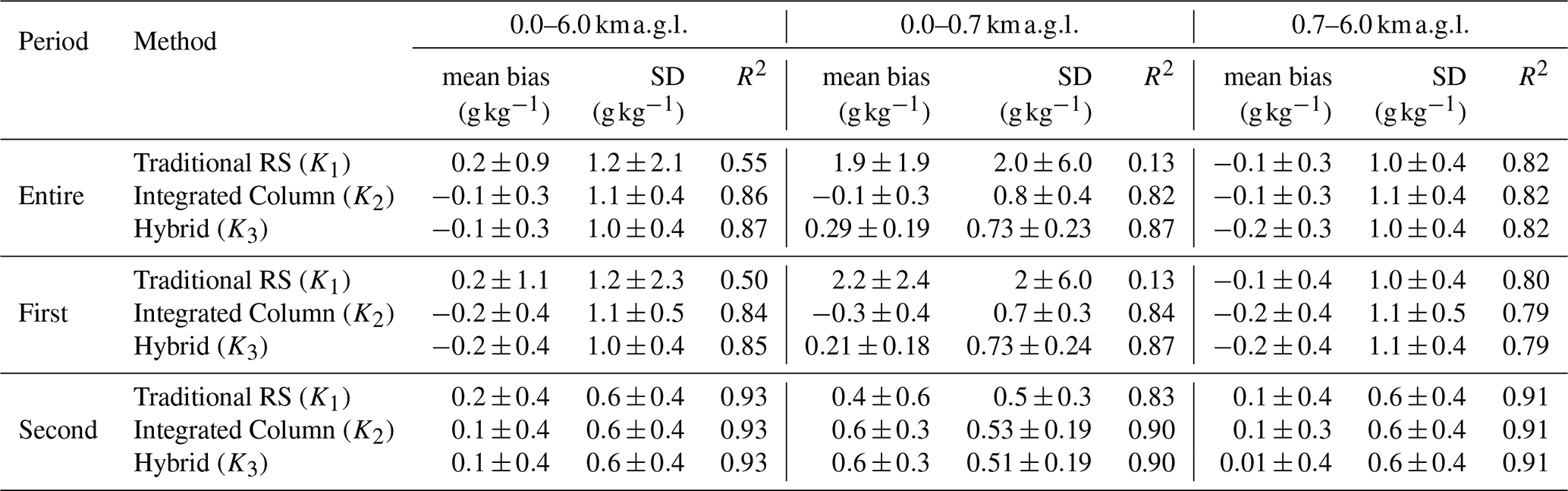
The comparison in Fig. 6, for the entire study period (2009–2022) and the entire profile (up to 6 $\mathrm{km}\mathrm{a}.\mathrm{g}.\mathrm{l}.$), reveals good agreement between calibrated lidar water vapour mixing ratio retrieved using different calibration methods – traditional RS (Fig. 6b), integrated column (Fig. 6h), and hybrid (Fig. 6o) – and the RS profiles. However, the best agreement was observed when using the hybrid method proposed (R²=0.87, slope=0.97, intercept of −0.06 g kg⁻¹, SD=1.0 ± 0.4 g kg⁻¹). The traditional RS-based method (R²=0.55, slope=1.13, $\text{intercept}=-\mathrm{0.21}$ g kg⁻¹, SD=1.2 ± 2.1 g kg⁻¹) and the integrated column method (R²=0.86, slope=0.94, $\text{intercept}=-\mathrm{0.01}$ g kg⁻¹, SD=1.1 ± 0.4 g kg⁻¹) showed less agreement (Fig. 6b and h). The best performance of the hybrid method is mainly due to the fact that it incorporates a correction for the incomplete overlap region, which improves the agreement between the calibrated lidar profiles and the RS measurements. When differentiating between different layers, negative differences in water vapour mixing ratio are observed in the range 0.7–4 $\mathrm{km}\mathrm{a}.\mathrm{g}.\mathrm{l}.$, while these differences become positive at higher altitudes (Fig. 6b, h, and o). Above 0.7 $\mathrm{km}\mathrm{a}.\mathrm{g}.\mathrm{l}.$, the mean differences confirmed the accuracy of all the methods in retrieving water vapour mixing ratio profiles using Raman lidar (with R²=0.82 for entire period and each method). Although some issues are observed, as the increase in SD with height (Fig. 6) which may be attributed to radiosonde drift caused by wind that can result in sampling different air parcels compared to lidar measurements, as well as increased noise in the lidar signal at higher altitudes (Brocard et al., 2013; Foth et al., 2015; Dai et al., 2018).

When separating the two different periods, Table 5 values suggest that the differences were more pronounced during the first period (Fig. 6d, j, and q), with mean bias values of 0.2 ± 1.1, −0.2 ± 0.4, and −0.2 ± 0.4 g kg⁻¹ for the traditional RS calibration, integrated column, and hybrid methods, respectively. This may be associated with the larger incomplete lidar overlap region in the first period that extended up to 700 $\mathrm{m}\mathrm{a}.\mathrm{g}.\mathrm{l}.$ In this region and over the complete study period, the traditional RS calibration method yielded a mean bias of 2.2 ± 2.4 g kg⁻¹, confirming an overestimation of water vapour relative to RS and lower reliability of lidar data below 0.7 $\mathrm{km}\mathrm{a}.\mathrm{g}.\mathrm{l}.$ (where R²=0.13). The R² values for the entire profile also confirm that differences were more significant during the first period (Fig. 6d, j, and q), with values of 0.50, 0.84, and 0.87, compared to the second period (Fig. 6f, m, and s), where the values were 0.93 for all methods.

Results from Table 5 and Fig. 6b, h, and o indicated a notable reduction in the discrepancies between lidar and RS within the incomplete overlap region for the hybrid and integrated column methods. Over the entire period, the traditional RS calibration method exhibited greater mean bias and SD compared to the integrated column and hybrid methods. Furthermore, R² improved from 0.13 to 0.87. The best agreement was obtained using the hybrid calibration method, which showed the lowest SD (0.73 ± 0.23 g kg⁻¹) and the highest R² (0.87). The positive bias observed in the hybrid method could result from the ERA5 model tendency to overestimate water vapour near the surface, as previously reported by Noh et al. (2016), Huang et al. (2021) and Zhu et al. (2022).

Although both the hybrid and integrated column methods generally provide good calibration constants and show good agreement between water vapour mixing ratio measurements from lidar and RS, the results in Table 5 do not show statistically significant differences between the two methods, perhaps due to the limited sample size of 31 simultaneous RS and lidar observations. However, it is important to note that W ranged from 0.5 to 25 mm, which corresponds to the typical range of minimum and maximum W registered at the Granada station (Vaquero-Martínez et al., 2023). Meteorological conditions can, however, influence the behaviour of water vapour profiles in the incomplete lidar overlap region and, consequently, in the W computation. Despite this, when analysing individual cases (Fig. 5), the hybrid methodology emerges as the most reliable method to calibrate Raman lidar water vapour measurements. This is because it can provide accurate vertical water vapour mixing ratio values in the lower layers (Fig. 5a, c, and d), allowing the detection of potential changes in the vertical structure of water vapour. This represents a significant advance in the correction of lidar measurements, which are often limited near the surface due to incomplete overlap. The detailed characterisation of water vapour variations near the surface, enabled by the hybrid method, offers an advantage over the integrated column method, which assumes constant water vapour values in this region, an assumption that is not always appropriate in the ABL (Fig. 5a, c, and d). The lower layers, more influenced by moisture processes, are prone to uncertainties when fitting the water vapour mixing ratio lidar profile to precipitable water vapour measurements from other instruments, highlighting the need to understand both the temporal and vertical behaviour of water vapour to accurately account for these variations. Furthermore, during periods with the largest incomplete overlap (until May 2017), assuming constant water vapour values can introduce greater uncertainties in determining the calibration constant (Fig. 2) compared to periods with a smaller incomplete overlap (from June 2017 onwards). In contrast, the hybrid method offers a more robust method, as demonstrated in Sect. 4.2 (Fig. 5). Additionally, the validation of the ERA5 model against RS data (Table 4 and Fig. 4) showed that the model can reproduce the behaviour of RS profiles in the incomplete overlap region, both during the day and at night, and across a wide range of meteorological conditions (148 profiles analysed from 2011–2023). These results suggest that the applicability of the hybrid methodology is largely independent of atmospheric conditions, avoiding the need for assumptions in this region (e.g., linear interpolation or the assumption of constant water vapour mixing ratio values).

4.4 High temporal evolution of Raman lidar calibration constants for water vapour measurements

The assessment of lidar water vapour mixing ratio against RS measurements demonstrated that the hybrid method can effectively address the limitations in evaluating the calibration constants because of the method significantly expands the number of available data due to the large temporal and spatial resolution of ERA5. Using the hybrid methodology (Eqs. 9 and 10), a dataset of calibration constants (K₃) with high temporal resolution was generated for the Raman lidar system. This methodology allows the calculation of a calibration constant for each uncalibrated lidar profile under cloud-free conditions and a high SNR response. This represents a significant advantage versus previous approaches for the our Raman lidar system when calibration was restricted only for short periods (e.g., Guerrero-Rascado et al., 2008; Navas-Guzmán et al., 2014). But the most remarkable is that the hybrid methodology significantly increases the number of calibrations, from 31 using radiosondes to 2300 using GNSS and model data. The obtained K₃ values were averaged to obtain monthly means, and their temporal evolution from 2009 to 2022 is shown in Fig. 7. The error bars represent the standard deviation of the monthly means. The vertical red band (lidar) and grey band (GNSS) indicate data gaps because there were no lidar measurements until June 2009 and in the period June 2014–May 2015. Also, there were no GNSS measurements between August 2019 and April 2020.

Figure 7 shows three different periods in terms of K₃ values that are similar to those observed in Fig. 2. These periods correspond to changes in the lidar system configuration, as discussed in Sect. 2.2, which are reflected in the variations of K₃ values. In general, the monthly mean calibration constants exhibited low standard deviations, supporting the reliability of the hybrid methodology and highlighting its potential for continuous evaluation of the calibration constant. The relative SD associated with each individual K₃ value was averaged to obtain the mean relative SD (2.4 %), which suggests low variability and supports the feasibility of the hybrid calibration methodology. We note that previous studies have shown that typical uncertainties in K estimation range from 2 % to 5 % when using high precision collocated radiosondes (e.g., Sherlock et al., 1999a; Mattis et al., 2002; Whiteman, 2003; Tratt et al., 2005; Reichardt et al., 2012; Froidevaux et al., 2013; Navas-Guzmán et al., 2014; Sica and Haefele, 2016; Martucci et al., 2018; Kulla and Ritter, 2019; Di Girolamo et al., 2020). In contrast, Brocard et al. (2013); Foth et al. (2015); Stachlewska et al. (2017); Dai et al. (2018) reported standard deviations in K close to 14 % when using the method based on precipitable water vapour, assuming constant water vapour mixing ratio values within the incomplete overlap region. Therefore, it can be concluded that the hybrid methodology applied at the AGORA station allows for the generation of high temporal resolution K values with high precision.

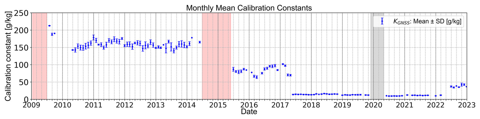
Figure 7 Temporal evolution of the monthly mean calibration constants from 2009 to 2022 over Granada. The error bars indicate the standard deviation. The shaded rectangles correspond to gaps in the lidar (red) or GNSS (grey) measurements.

The high temporal resolution of K₃ permits a detailed evaluation of the Raman lidar system. Results from Fig. 7 show that the K₃ values were initially higher in 2009. For the period 2011–2013, great stability in K₃ was observed, with mean value of 159 ± 9 g kg⁻¹ (6 %). From 2015 to May 2017, K₃ ranges from 64 ± 3 g kg⁻¹ (5 %) to 102 ± 2 g kg⁻¹ (2 %), before decreasing to 15.0 ± 1.0 g kg⁻¹ (6 %) in June 2017. However, the hybrid methodology reveals that these changes in K₃ are smooth and can be tracked. During the subsequent period (June 2017–2021), the average K₃ was 13.0 ± 2.0 g kg⁻¹, with values ranging from a minimum of 9.4 ± 0.6 g kg⁻¹ to a maximum of 16.6 ± 0.9 g kg⁻¹. In May 2022, the average increased to 38 ± 3 g kg⁻¹, but the low standard deviations allow again for effective tracking of changes in calibration constants. Although significant changes in K₃ are evident across different stages of its temporal evolution, the low standard deviations in the monthly means suggest a more stable and reliable system, linked to the optimisations made to our Raman lidar. Nevertheless, the high temporal resolution of K₃ allows for appropriate corrections in water vapour mixing ratio retrievals and facilitates the detection of potential system changes, such as photomultiplier tube deterioration or dichroic mirror degradation.

4.5 Temporal evolution of water vapour mixing ratio profiles during different case studies

The proposed hybrid methodology applied to the Raman lidar (Sects. 3.3 and 4.2) permits continuous analysis of the water vapour at the UGR station for a period of 14 years (2009–2022). Figure 8 illustrates four examples of the temporal evolution of water vapour mixing ratio profiles for different seasons and atmospheric conditions. The examples correspond to nighttime observations on 18 August 2016, 15 May 2017, 28 January 2021, and 1 September 2022. Temporal resolution is 30 min and the vertical resolution is 7.5 m. Figure 8 shows the potential of the hybrid method applied to the Raman lidar system to obtain continuous water vapour mixing ratio profiles, allowing for detailed characterisation of water vapour variations in the troposphere with high temporal and vertical resolution. Results from Fig. 8 also highlight the importance of monitoring water vapour variability with time and height because it effectively captures different structures both within the ABL and in the free troposphere. Moreover, the most relevant issue is that the hybrid methodology can address the limitations of lidar data in the incomplete overlap region.

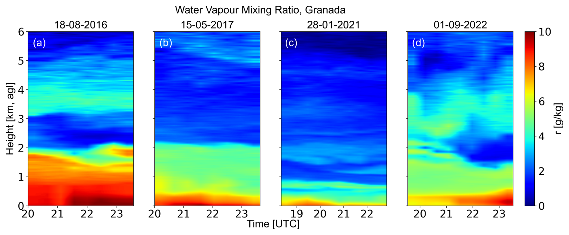
Figure 8 Temporal evolution of water vapour mixing ratio profiles over Granada on 18 August 2016 (a), 15 May 2017 (b), 28 January 2021 (c), and 1 September 2022 (d).

Figure 8 shows that the case with the highest water vapour mixing ratio is in summer on 18 August 2016 (Fig. 8a), while the case in winter on 28 January 2021 (Fig. 8c) exhibited the lowest; the other two cases in spring/autumn present intermediate values of water vapour and they are similar to each other. This seasonal pattern is consistent with the findings from the statistical analysis of water vapour at Granada reported by Navas-Guzmán et al. (2014). Additionally, to better understand the observed variations in water vapour, geopotential height maps at different atmospheric levels (data analysed from the NCEP/NCAR reanalysis model, https://psl.noaa.gov/data/composites/hour/, last access: 11 May 2026) can additionally be used to understand the atmospheric conditions. Five day backward trajectories were also analysed using the NOAA HYSPLIT model (https://www.ready.noaa.gov/hypub-bin/trajtype.pl?runtype=archive, last access: 11 May 2026). Note that maps and backwards trajectories are not shown for clarity.

On 18 August 2016 water vapour mixing ratio profiles (Fig. 8a) showed three different decoupled layers: a humid layer extending up to 2 $\mathrm{km}\mathrm{a}.\mathrm{g}.\mathrm{l}.$, with water vapour mixing ratio values decreasing from 10 to 4 g kg⁻¹; a dry layer between 2.0 and 3.0 $\mathrm{km}\mathrm{a}.\mathrm{g}.\mathrm{l}.$, where water vapour decreases from 3 to 1.5 g kg⁻¹; and another humid layer above 3 km, characterised by an increase in water vapour from 1.5 to 4 g kg⁻¹. Additionally, the temporal evolution shows that heights at which water vapour mixing ratio exceeds 6 g kg⁻¹ decrease with time, being observed at 1.8 $\mathrm{km}\mathrm{a}.\mathrm{g}.\mathrm{l}.$ at 20:00 UTC and descending to 1.45 $\mathrm{km}\mathrm{a}.\mathrm{g}.\mathrm{l}.$ by 23:00 UTC. For this day, the geopotential height maps indicated an extratropical low-pressure system over the Bay of Biscay, with an associated cold front that extended southward to 30° N. The southwesterly winds associated with the cold front may favour the advection of humid air from the North Atlantic toward the Iberian Peninsula. The instability linked to this type of system may have contributed to the decoupling of atmospheric layers observed in Fig. 8a. Backward trajectory analysis indicated that air masses reaching Granada originating in the North Atlantic.

The case on 15 May 2017 (Fig. 8b) shows a moist layer near the surface, with water vapour mixing ratio values reaching up to 10 g kg⁻¹, and a well-mixed layer between 0.7 and 2.0 $\mathrm{km}\mathrm{a}.\mathrm{g}.\mathrm{l}.$, characterised by slight variations in water vapour with height. Above this layer, the water vapour content gradually decreases up to 5 $\mathrm{km}\mathrm{a}.\mathrm{g}.\mathrm{l}.$, with values ranging from 4 to 1.8 g kg⁻¹. At greater heights, a layer that can be considered moist for those heights is observed, with water vapour mixing ratio values around 4 g kg⁻¹. The analysis of synoptic conditions indicates the influence of an anticyclonic system over the Iberian Peninsula, followed by a dissipating cold front. The winds resulting from the interaction between these systems are likely to favour the advection of moist air from the Atlantic. This is confirmed by the backward trajectory analysis with air masses originating in the North Atlantic. The dissipating cold front supports the formation of stratiform clouds, including low clouds and cirrus, as observed in satellite images provided by the Cooperative Institute for Meteorological Satellite Studies (CIMSS, https://tropic.ssec.wisc.edu/archive/, last access: 11 May 2026). These high clouds may be related to the humidity values observed above 5 $\mathrm{km}\mathrm{a}.\mathrm{g}.\mathrm{l}.$

A marked anticyclonic influence was observed on 28 January 2021. This situation is indicative of stable atmospheric conditions, with an air mass characterised by low water vapour content, as shown in Fig. 8c. Water vapour mixing ratio values were less than 7 g kg⁻¹ and were mostly found in the first kilometre. This concentration in the lower layer can be attributed to atmospheric stability, which limits vertical mixing. Above this layer, the values gradually decreased to 1 g kg⁻¹ at 5 km, and further upward, they approached zero, reflecting the typical pattern of decreasing moisture with height.

Finally, on 1 September 2022 (Fig. 8d), strong winds at mid and high levels (300 and 200 hPa, approximately 9.5 to 12 $\mathrm{km}\mathrm{a}.\mathrm{s}.\mathrm{l}.$) were observed in the wind maps, resulting from the interaction between a trough extending from a low geopotential centre over western Ireland and a high geopotential centre over northern Africa. The presence of strong winds at altitude can lead to convection and instability, resulting in low and middle cloudiness, as observed in satellite images analysed by CIMSS, graphs are not shown for brevity. This may explain the presence of humid layers in this case (Fig. 8d), with the first layer extending up to 2 $\mathrm{km}\mathrm{a}.\mathrm{g}.\mathrm{l}.$, where the water vapour mixing ratio values decrease from 9 to 3 g kg⁻¹, and a second layer between 2.5 and 4.0 $\mathrm{km}\mathrm{a}.\mathrm{g}.\mathrm{l}.$, with water vapour values decreasing from 5 to 3 g kg⁻¹. Additionally, a dry layer appeared around 21:00 UTC, with values decreasing to 1 g kg⁻¹, positioned between the two previously mentioned decoupled humid layers. This decoupling may have been caused by atmospheric instability.

5 Summary and Conclusions

In this study, a hybrid methodology has been presented that allows obtaining high temporal resolution calibration constants for Raman lidar measurements and the subsequent retrieval of improved accuracy water vapour mixing ratio profiles. This methodology was developed to optimise the retrieval of water vapour measurements using the Raman lidar, which operated at the UGR urban station and is part of the EARLINET/ACTRIS network. During the period 2009–2022, only 31 correlative radiosondes were available for direct intercomparisons, significantly limiting the evaluation using calibration constants K through traditional RS-based methods. Another method to obtain K is based on precipitable water vapour (W) measured by collocated remote sensing instruments. Nevertheless, this integrated method faced the particular difficulty of an incomplete overlap region that varies over time, ranging between 700–300 $\mathrm{m}\mathrm{a}.\mathrm{g}.\mathrm{l}.$ We highlighted that the classical assumption of constant values for water vapour is not always appropriate in the Atmospheric Boundary Layer (ABL), particularly in conditions of atmospheric instability.

The new hybrid method exploits correlative W measurements, which significantly increase the number of calibration cases, and optimise the lidar profile in the incomplete overlap region by incorporating the water vapour mixing ratio shape provided by the NWP model. The first optimisation step of this methodology involved assessing which instrument provided the most reliable estimates of W; to this end, correlative measurements were evaluated. The dataset now includes 73 simultaneous RS measurements collected during both daytime and nighttime. The best agreement with RS was found for GNSS measurements (determination coefficient of 0.95, mean bias of −0.74 ± 1.2 mm, and relative difference of −4 %), and therefore GNSS W was chosen as the reference. For the optimisation of the most appropriate NWP we again performed evaluations of ERA5, CAMS and MERRA-2 versus radiosondes. Now the database for the intercomparisons was even larger with 148 simultaneous RS, both at daytime and nighttime, and the ERA5 model was selected for correcting the lidar profile within the lidar incomplete overlap region, due to its higher temporal and spatial resolution. The mean bias and standard deviation between ERA5 and RS in the first 0.7 $\mathrm{km}\mathrm{a}.\mathrm{g}.\mathrm{l}.$ were 0.13 ± 0.15 and 1.16 ± 0.08 g kg⁻¹, respectively, indicating strong agreement.

The Raman lidar system was first calibrated using traditional methods by intercomparisons with the 31 available collocated radiosondes. Significant changes in K with time were observed for the entire period 2009–2022, but with very low temporal resolution due to the few RS available. This issue was addressed through the development and application of the hybrid calibration method, which expanded the number of available measurements to over 2000 for the entire period, making it possible to accurately evaluate the performance of our Raman lidar system and detect how the changes in the system affected the calibration constants K. The hybrid methodology was evaluated against the 31 simultaneous RS nighttime measurements, indicating that the new method significantly reduces biases and discrepancies compared to traditional RS calibration methods in the incomplete lidar overlap region. Specifically, in the incomplete overlap region, the mean bias and SD were 0.29 ± 0.19 and 0.73 ± 0.23 g kg⁻¹ (hybrid method), with R² 0.87. Thus, the hybrid methodology ensures more robust and consistent measurements of water vapour mixing ratio profiles, enabling the detection of potential changes in the vertical structure of water vapour, regardless of atmospheric conditions. The detailed characterisation of water vapour variations near the surface, made possible by the hybrid method, offers an advantage over the integrated column method, which assumes constant water vapour values in this region, an assumption that is not always appropriate in the ABL. This assumption can introduce uncertainties when fitting the water vapour mixing ratio lidar profile to W measurements from other instruments, as these layers tend to have higher humidity.

Once the instrument was appropriately calibrated, the hybrid methodology was applied to the period 2009–2022, enabling the creation of a unique database of water vapour mixing ratio profiles in the region. Several case studies demonstrate the capabilities of the our Raman lidar system to obtain high temporal resolution profiles of water vapour mixing ratio under different seasonal and atmospheric conditions. These cases highlight the potential of this technique to describe vertical variations of water vapour in the troposphere and underscore the importance of understanding water vapour variability over time and altitude. The hybrid methodology could be used to generate additional water vapour datasets from instruments within the EARLINET/ACTRIS network that were originally designed for aerosol measurements. In addition, this work will contribute to the objectives of the new COST Action European Atmospheric Research LIdar COoperation on Science and Technology (EARLICOST, CA24135), which aims to enhance water vapour retrieval capabilities. Therefore, it represents a step forward in the state of the art of lidar water vapour calibration methods, opening new possibilities for water vapour data assimilation in NWP, and ultimately enhancing the scientific community's capabilities in weather forecasting, understanding the impact of water vapour on direct radiative forcing, as well as the role of water vapour in cloud formation and aerosol hygroscopic growth.