Arctic Weather Satellite assessment and assimilation at ECMWF

The Arctic Weather Satellite (AWS) is a ground-breaking small satellite from ESA. Its goal is to measure microwave sounding radiances of sufficient quality for improving weather forecasts from a rapidly developed, low-cost mission. AWS is a pathfinder for the proposed EUMETSAT Polar System (EPS) Sterna constellation, which would represent a paradigm shift for operational satellite meteorology. The payload of AWS is a newly developed passive microwave (MW) sounder, with traditional temperature and humidity sounding channels near 50 and 183 GHz, plus novel humidity sounding channels near 325 GHz. In this paper, first the radiometric performance of AWS is evaluated in reference to the ECMWF data assimilation system and heritage sounders, and then assimilation trials are presented to gauge the impact of AWS on forecast performance. The assimilation of AWS follows the all-sky method as applied to other MW radiometers in the ECMWF system, with the notable addition of the first-ever sub-millimetre wavelengths from the 325 GHz channel suite. Channel biases and noise estimates are generally in line with those of heritage instruments; AWS performance is similar to that of equivalent channels of AMSU-A and MWHS-2 in the 50 and 183 GHz bands, respectively, but effective noise for temperature sounding is higher than that of ATMS after spatial averaging. Nine months of experimentation show that adding AWS to the assimilation improves short-range forecasts of humidity, winds, and temperature. Geopotential height and winds are improved in the Southern Hemisphere through day 4. Despite its small size, AWS is a high-performing radiometer with data quality sufficient for operational assimilation in NWP. It has been assimilated operationally at ECMWF since July 2025.

1 Introduction

Microwave sounders are a key pillar in the global observing system of meteorological satellite instruments. Simply put, the assimilation of microwave sounder radiances leads to improved weather forecasts globally (Duncan et al., 2021) as well as for extreme events (Magnusson et al., 2025) in the ECMWF Integrated Forecasting System (IFS), and this is also seen in machine-learning based systems (Laloyaux et al., 2025). The number of microwave sounders in orbit has been limited, but if more of these sensors could be flown then we should expect further improvements in forecasts (Lean et al., 2025; Rivoire et al., 2024).

In recent years, a raft of “new space” concepts has swept through satellite meteorology, bringing increased miniaturisation of instruments, independent platforms, and rapidly deployed new technology (Stephens et al., 2020). This has led to numerous low-cost demonstration missions in space, but has not yet led to missions that meet the stringent operational requirements for use in numerical weather prediction (NWP) in terms of radiometric stability, data latency, and overall lifetime. For passive radiances, most NWP centres exclusively assimilate data from the bus-sized platforms that typify the old paradigm of large, heavily instrumented satellites.

The Arctic Weather Satellite (AWS) from ESA is a relatively low-cost mission about the size of a washing machine (Voosen, 2024). Measuring about one cubic metre and weighing 125 kg, AWS has a microwave radiometer as its sole payload. It was launched on a ride-share rocket in August 2024, just 36 months after the original contracts were signed, typifying the new space concept despite being agency-led. AWS serves as a pathfinder and proto-flight model for the proposed EUMETSAT Polar System (EPS) Sterna constellation, which would fly pairs of AWS-class satellites in three orbits to complement the so-called “baseline” orbits of 01:30, 05:30, and 09:30 (local solar time at the equator for sun-synchronous orbits) agreed by the Coordination Group for Meteorological Satellites (CGMS) for operational microwave and infrared sounding instruments.

The goal of AWS is to observe operational-quality radiances from a small, rapidly developed, and low-cost mission. With this in mind, this paper will assess the radiometric performance of AWS and explore its impact on forecast quality in a global NWP system. The paper is structured as follows: the AWS instrument and relevant aspects of data pre-processing at ECMWF are introduced in the next section; Sect. 3 briefly explains all-sky assimilation and then the NWP-based method of assessing the radiometric performance of microwave sounders; Sect. 4 analyses the radiometric performance of AWS; Sect. 5 gives results on the forecast impact in the ECMWF system; the paper finishes with conclusions and some discussion.

2 Data

In this section, first the AWS radiometer is introduced with the details necessary for this study. For a more in-depth description of the instrument, see Eriksson et al. (2025). Second, we describe the observation pre-processing that is applied to AWS data prior to ingestion to the data assimilation system.

2.1 The AWS instrument and orbit

With 19 channels across four instrument feedhorns, AWS spans three key absorption bands for atmospheric sounding. These include temperature sounding near 50 GHz and humidity sounding near the 183 and 325 GHz water vapour absorption lines. Most of these channels are for atmospheric sounding, but there are also three window channels at 50.3, 89.0, and 165.5 GHz to aid in retrieval of surface properties. This channel complement (see Table 1) is similar to that of heritage instruments like the Advanced Technology Microwave Sounder (ATMS; Weng et al., 2012) or the combination of AMSU-A and MHS, but without lower-frequency window channels at 23 and 31 GHz and without channels sounding the mid and upper stratosphere.

Table 1 Specifications for centre frequency, bandwidth, footprint NEDT (noise equivalent differential temperature), and measured field of view (FOV) size for AWS. All channels have quasi-vertical polarisation (QV). The FOV is defined as the average diameter of the −3 dB ellipse at nadir. The NEDT values given are the specified requirements for maximum noise levels for the defined footprint size, rather than sample NEDT (see text). The last columns give the equivalent ATMS and MWHS-2 channel numbers, if applicable.

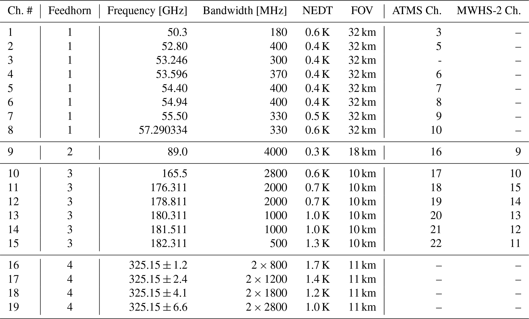
Some key differences between AWS and heritage MW sounders are worth noting. First, AWS holds the first channels above 300 GHz – sub-millimetre wavelengths and thus “sub-mm” channels – on an instrument intended for near-real time, operational use (Duncan et al., 2025b); these channels provide unprecedented sensitivity to atmospheric ice mass and presage the capabilities of the next-generation Ice Cloud Imager (ICI) from EUMETSAT (Eriksson et al., 2020), expected to launch in 2026. Second, to enable a compact design and save weight, the AWS radiometer does not use a quasi-optical network with beam co-alignment, which many heritage instruments rely upon to co-locate all channels (Albers et al., 2023). This means that the four feedhorns of AWS point in slightly different directions, leading to disparate geolocations, incidence angles, and swaths on the ground between channel sets. Third, AWS 183 GHz channels feature single-sidebands, whereas on heritage sounders these channels typically feature dual-sidebands. This instrument design choice does not significantly impact the geophysical characteristics, and herein we consider them equivalent for sake of comparison, e.g. 183.31 ± 3 GHz on ATMS and 180.31 GHz on AWS.

AWS was designed to fly in a variety of sun-synchronous and low-inclination orbits, as the specifications for the EPS-Sterna constellation had not yet been determined. From the ride-share launch in August 2024, AWS was inserted into a 22:30 local time (LT) of the ascending node (LTAN) sun-synchronous orbit. This puts it slightly after the Metop series at 21:30 LT and before the operational NOAA satellites at 01:30 LT on their descending node. During the first months of AWS there were three legacy NOAA satellites in drifting sun-synchronous orbits (NOAA-15, -18, -19), but these were decommissioned in June 2025. Figure 1 demonstrates the importance of orbital crossing times for sounder data, putting AWS observations in the context of cross-track sounder radiances used operationally at ECMWF in a given 90-minute window in late 2025.

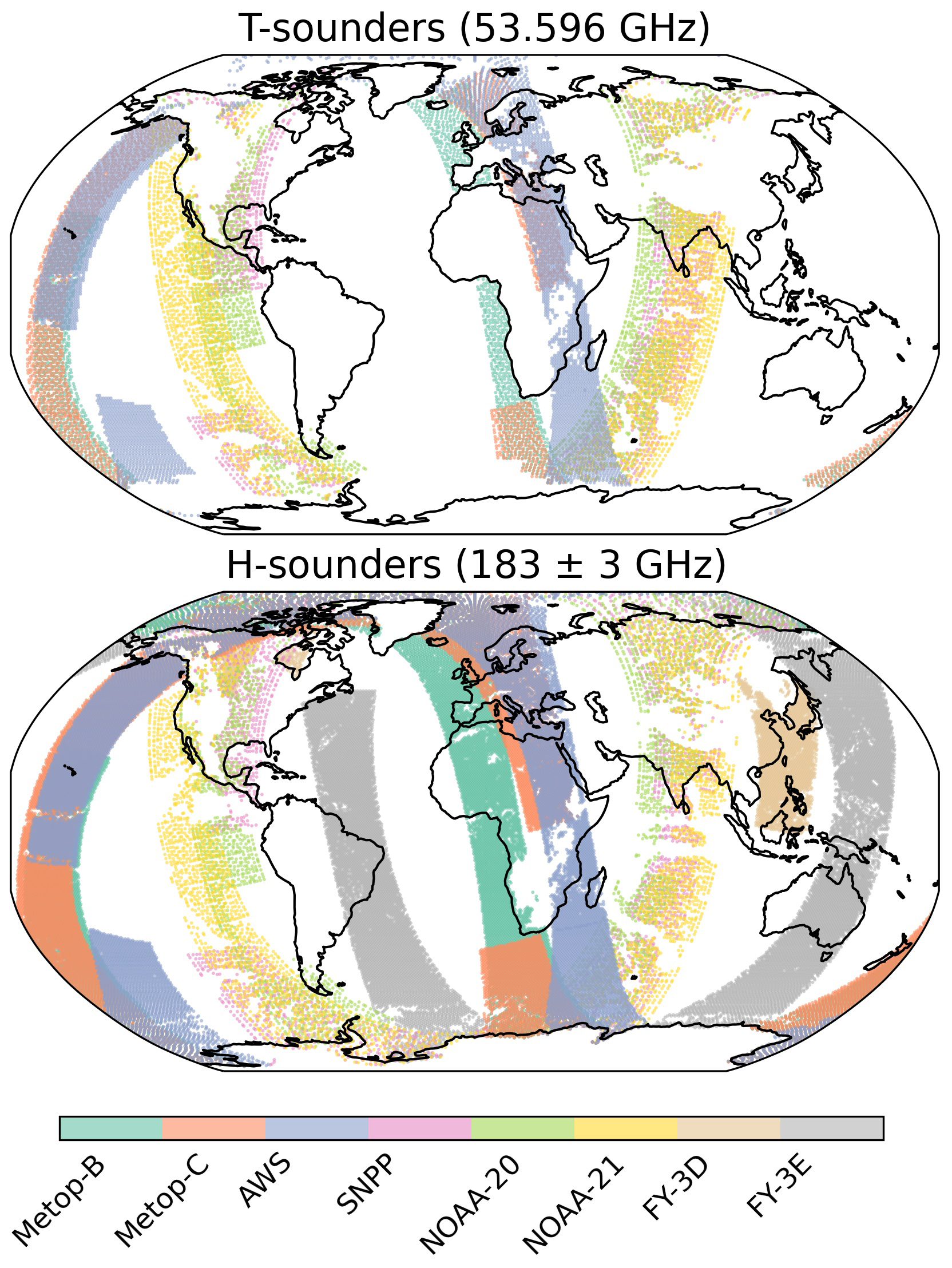
Figure 1 Data assimilated from cross-track MW sounders in the last 90 min of the 12:00Z long-window assimilation, 19:30–21:00Z on 3 December 2025, from ECMWF operations. The top panel shows used data points from temperature sounders with a 53.596 GHz channel (equivalent to AWS 4); the bottom panel shows the same for the 183 ± 3 GHz humidity sounding channels (equivalent to AWS 13 at 180.31 GHz). Colours indicate the satellite platform. 183 GHz channels from conical scanners are excluded here.

AWS orbits at approximately 600 km altitude, lower than the Metop and NOAA platforms at about 830 km. This lower altitude allows for relatively small field of view (FOV) sizes on the ground, with 10 km FOVs achieved at the higher frequencies from an antenna with effective diameter of only 0.16 m. Linked to its lower orbiting altitude, to achieve a roughly 2000 km swath width from all feedhorns, AWS observes out to scan angles of 54.5°, greater than the 52.725 of ATMS or 49.44 of MHS, for example. This leads to larger zenith angles that can reach 70° in some cases.

The AWS scan pattern features higher incidence angles at swath edge and greater spatial oversampling along- and across-track than most heritage instruments. AWS rotates at 50.4 rpm, producing 145 Earth-view samples per scan line in 110° of scan angle from a 2.5 ms integration time, and the near-nadir cross-track samples are separated by about 8 km. We can contrast this with ATMS, which samples with 16 km scan spacing and 90 spots per scan. An illustration of the differing swaths and the FOV variation across the scan can be seen in Fig. 2. This figure also displays the different geolocations of the four feedhorns.

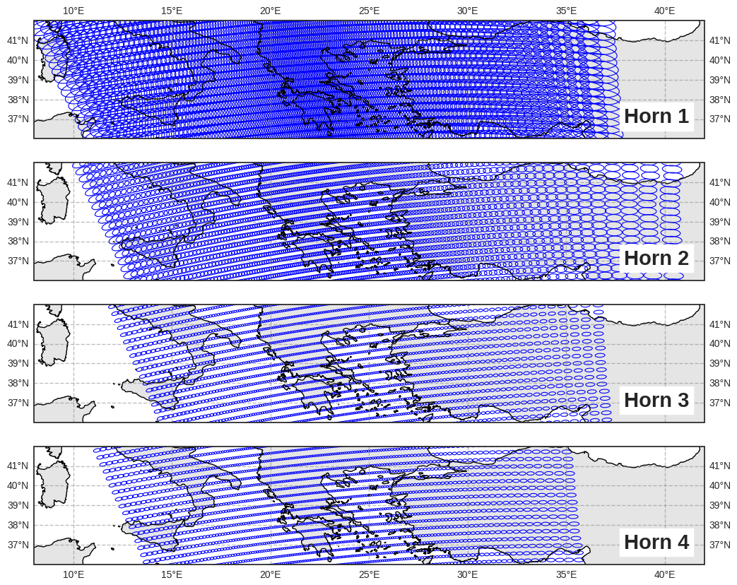
Figure 2 Approximate FOV sizes for each feedhorn of AWS at the −3 dB power contour. All scan positions are shown but only every 5th scan is plotted for clarity. This means that in practice even feedhorns 3 and 4 are over-sampled along track.

2.2 AWS pre-processing at ECMWF

Due to the different geolocations of the feedhorns on AWS, a method is needed to bring the observations together into a single observation vector. Although this is not strictly necessary, it is what data assimilation systems and radiative transfer models are built to handle, and it provides certain scientific synergies such as allowing lower frequencies to retrieve the surface emissivity for higher frequencies that have less surface sensitivity.

The problem of co-locating the AWS fields of view is solved by superobbing onto a common equal-area grid of around 50 km. Superobbing is a method to spatially average the original observations (Geer et al., 2010; Duncan et al., 2024a), with the feedhorn geolocations determining which box a given observation is assigned to. It is a simple average, with antenna response patterns disregarded. Once each feedhorn has been averaged separately, we can build 19-channel observation vectors at a single geolocation due to the exact spatial matches, i.e. match the horns together. At swath edges where not all horns overlap, superobs may be populated by one or two horns only (for example over western Sicily in Fig. 2). Zenith angle information is retained on a per-feedhorn basis, which is necessary for realistic simulation of the radiances. The superobbing and horn-matching method simplifies downstream processing, reduces data volume considerably, and importantly reduces representation errors (Janjić et al., 2018) for later assimilation. For example, 35 AWS observations can be averaged together into one 50 km superob in the middle of the swath; this also has a significant impact on effective instrument noise, as we will see later.

Superobbing AWS radiances to 50 km resolution follows the method applied to other humidity sounders MHS and MWHS-2 for assimilation in the IFS (Duncan et al., 2024a). In contrast, the temperature sounder AMSU-A has much larger footprints and thus its observations are not superobbed. For ATMS, it is currently assimilated in clear-sky conditions only after 3 × 3 superobbing (Bormann et al., 2013), and remains assimilated by this method in experimentation herein. However, for comparisons of radiometric behaviour in this paper, ATMS is treated as AWS, i.e. 50 km superobs in all-sky conditions.

3 Method

The assessment of AWS radiometric performance is done in reference to the ECMWF data assimilation system, which compares hundreds of millions of observed radiances with model equivalents from a short-range forecast (i.e. computes O–B) on a daily basis. The model background (B) in observation space provides a tight constraint on expected radiometric behaviour of MW sounder observations (O), with model fields interpolated to the observation location in time and space and simulated by the forward model, providing a realistic 3D snapshot of all radiatively significant species in the profile. Background errors at MW sounder frequency bands range from about 0.1 to 1 K in clear skies; due to larger errors over complex surfaces and in areas of thick cloud or precipitation, this method avoids such scenes where appropriate.

In this section, first the relevant elements of the all-sky microwave radiance assimilation at ECMWF are briefly discussed. Second, aspects specific to AWS assimilation are described. Third, the method for assessing instrument performance using the NWP background is given for microwave sounders.

3.1 All-sky microwave radiance assimilation at ECMWF

This section briefly describes newer developments of all-sky assimilation at ECMWF and those relevant for the remainder of the paper. Fuller descriptions of the all-sky assimilation method can be found elsewhere in the literature (e.g Geer et al., 2010, 2014; Duncan et al., 2022), as well as in the official IFS documentation (ECMWF, 2024).

All-sky radiance assimilation is underpinned by a radiative transfer model that simulates the effects of clouds and precipitation in addition to atmospheric gases. In this study we use RTTOV-SCATT version 13.2, which importantly includes updated scattering properties of frozen hydrometeors (Geer et al., 2021) and the SURFEM-Ocean emissivity model over sea (Kilic et al., 2023). Both of these developments were done with the advent of sub-mm radiances in mind, and are included in the IFS version used in this study, Cycle 49r1 (ECMWF, 2024). In addition, RTTOV-SCATT takes as input ozone profiles from the IFS (rather than climatological profiles), which is important for AWS due to non-negligible ozone sensitivity for sub-mm frequencies (Duncan et al., 2024b; Eriksson et al., 2025). Lastly for radiative transfer, RTTOV uses the measured spectral response functions (SRFs) from laboratory measurements of AWS to compute absorption coefficients.

To assimilate radiances from cloudy and precipitating scenes, the IFS uses a symmetric observation error model (Geer and Bauer, 2011) that equally weights observed and modelled cloud amounts when determining the observation error. This relies on a cloudiness proxy to indicate clear-sky and cloudy scenes, as representation error is the main driver of all-sky observation errors and this is highly correlated with cloudiness. Whereas heritage sounders like AMSU-A and MHS use window channel differences for cloud proxies (Geer et al., 2014; Duncan et al., 2022), AWS lacks the low-frequency channels used by AMSU-A and also has a new sub-mm channel set that may need a different approach. Thus a useful indicator of cloudiness for AWS is the cloud impact (CI; see Eq. 1), which has been used previously in the infrared (Okamoto et al., 2014). CI is defined as

$$\begin{array}{}\text{(1)}& \text{CI}=\left|(O-\text{BiasCorr})-B_{\mathrm{clr}}\right|/\mathrm{2}+\left|B-B_{\mathrm{clr}}\right|/\mathrm{2}\end{array}$$

with B denoting the short-range forecast in observation space (i.e. model background), simulated for both all-sky conditions and in clear-sky (B_clr). A bias correction term (BiasCorr) is included from the variational bias correction (VarBC) scheme (Dee, 2004) to remove systematic offsets between observations (O) and model.

3.2 Assimilation aspects specific to AWS

In general, the assimilation of AWS radiances in the IFS follows the methods in place for AMSU-A and humidity sounders MHS and MWHS-2 (Duncan et al., 2022; Lawrence et al., 2018; Duncan et al., 2024a). However, three aspects of AWS require additional methodological consideration: its lack of low-frequency channels for liquid water path (LWP) retrieval, its novel 325 GHz channels, and the dependency of effective instrument noise on scan position due to superobbing. These are covered here in order.

As defined above, CI is a relatively simple way to define cloudiness in terms of brightness temperatures (TBs). As investigated by Lean et al. (2023), the lack of 23.8 and 31.4 GHz low-frequency window channels relative to AMSU-A does not hinder assimilation of the 50 GHz sounding band in all-sky conditions. Instead of LWP, we use the cloud impact at AWS channel 2 (CI₂; equivalent to AMSU-A channel 4) to guide the observation error model for channels 4 to 7. In Fig. 3, the left panels show the observation error models for the AWS temperature sounding channels on horn 1 as a function of CI₂. AWS uses CI over both land and sea, in contrast to AMSU-A, which uses LWP over sea and scattering index (SI) over land. Following the all-sky implementation of instruments like AMSU-A, the observation error models shown have been determined empirically by the behaviour of O–B standard deviations as a function of the symmetric cloud proxy. For 183 GHz channels, the SI approach of Geer et al. (2014) is retained, using a difference of AWS channels at 89 and 165.5 GHz (see middle panels in Fig. 3).

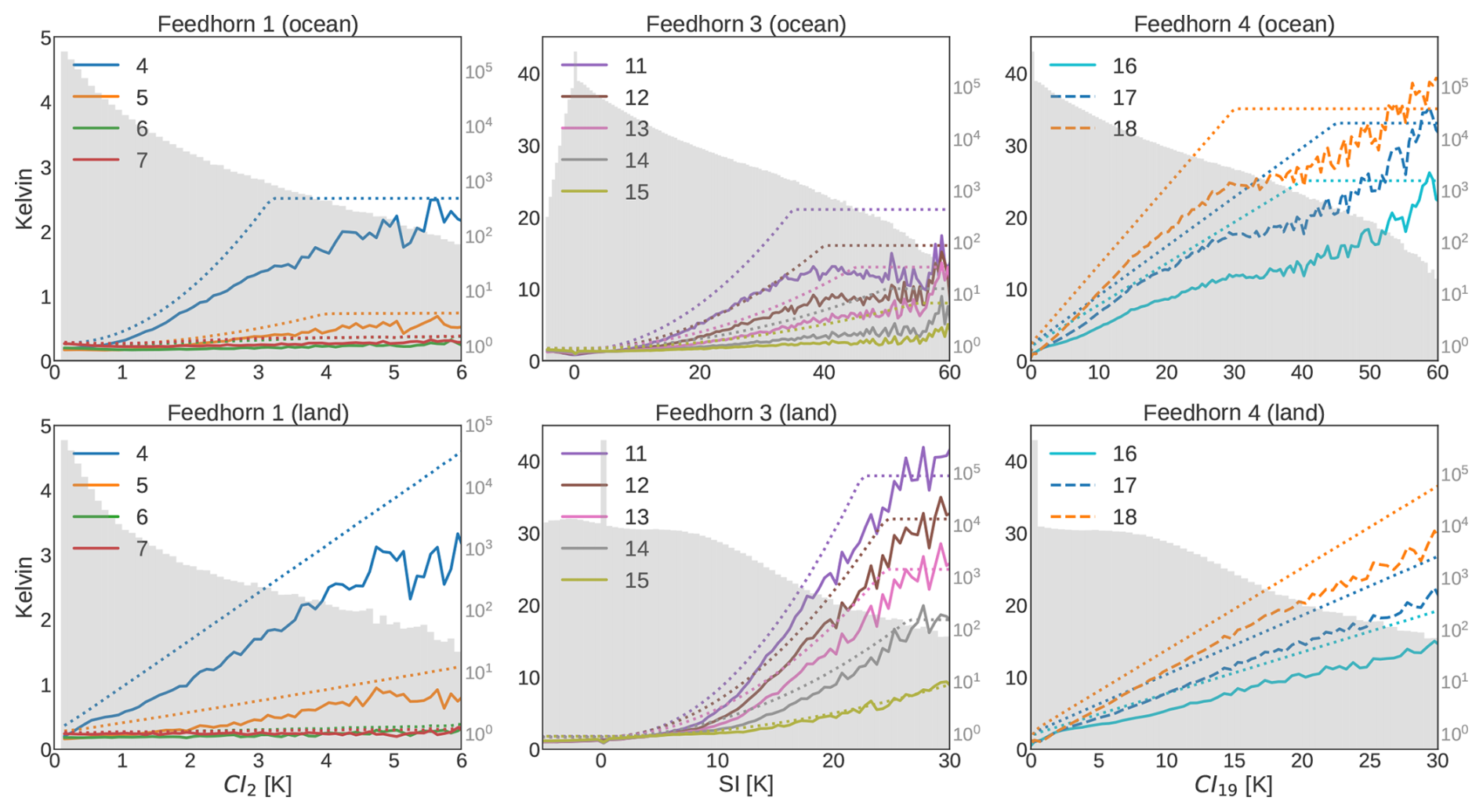
Figure 3 Observation error models (dotted lines) and standard deviation of background departures (SD(O−B); solid and dashed lines) for assimilated AWS channels. Panels are split into assimilated channels from horns 1 (left), 3 (middle), and 4 (right), with sea on top and land on bottom. Data cover assimilated observations from 29 October to 12 November 2025. Grey bars illustrate the number of observations per CI or SI bin. Here SI is the symmetric scattering index, following Geer and Bauer (2011).

The novel 325 GHz humidity sounding channels on AWS have greater sensitivity to ice particle scattering than 183 GHz channels, and it follows that the cloud proxies previously used at 183 GHz may not be sufficient at sub-mm frequencies. Lean and Bormann (2024) analysed this in detail and determined that a CI-based approach was preferred, using the lowest-peaking 325 GHz channel (19 on AWS). CI₁₉ is thus used for the observation error model of 325 GHz channels over both land and sea, with values seen in the right panels of Fig 3. In terms of quality control decisions, 325 GHz channels follow exactly what is done for 183 GHz channels with equivalent sensitivity (e.g. channel 18 is treated the same way as channel 13; see Geer et al., 2022).

Superobbing decreases effective instrument noise in a way that is significant for temperature sounding channels but largely negligible for humidity-sensitive frequencies (Duncan et al., 2024a). This is because background errors for temperature sounding channels are an order of magnitude smaller than those of humidity sounding and window channels, with sample NEDT typically larger than background errors. When employing grid-based superobbing, cross-track sounders like AWS achieve greater noise reduction where more observations are averaged together. Near the middle of the swath roughly 30 observations are averaged together and thus noise is greatly reduced near nadir, compared to little noise reduction at scan edge where perhaps only 2 or 3 observations constitute one superob.

With effective instrument noise a key driver of observation errors, it becomes necessary to augment the all-sky observation error model for superobbed temperature sounding channels on cross-track instruments. Here we use zenith angle as a proxy for the number of observations per superob, and define a noise term (σ_zen) that is scaled as a function of the zenith angle in radians (θ), given in Eq. (2). This term is added in quadrature to the total observation error as output by the standard all-sky error model in clear or cloudy conditions (σ_clr+cld), seen below in Eq. (3).

$$\begin{array}{}\text{(2)}& {\displaystyle }{f}_{\mathrm{scale}}\left(\mathit{\theta }\right)=\mathrm{0.1}+\mathrm{0.9}\exp (-\mathrm{0.8}{\mathit{\theta }}^{\mathrm{2}})\text{(3)}& {\displaystyle }{\mathit{\sigma }}_{\mathrm{total}}=\sqrt{{\mathit{\sigma }}_{\mathrm{clr}+\mathrm{cld}}^{\mathrm{2}}+{\left({\mathit{\sigma }}_{\mathrm{zen}}/f\left(\mathit{\theta }\right)\right)}^{\mathrm{2}}}\end{array}$$

This error model augmentation is applied to AWS channels 4 to 7, with σ_zen ranging from 0.10 to 0.14 (see Table 11 in Duncan et al., 2025a). The values for σ_zen and the functional form for f_scale were determined empirically from statistics of O–B standard deviations as a function of scan position, endeavouring to flatten the curve and improve Gaussianity of normalised departures overall. As formulated, the additional term causes no inflation at nadir and produces enough inflation at scan edges to account for greater effective noise in superobs with fewer observations.

3.3 Performance assessment via NWP departures

3.3.1 Screening definitions

Assessment of radiometric performance via NWP departures is not a new concept (e.g. Bell et al., 2008; Lawrence et al., 2018; Newman et al., 2020). But previous methods have relied upon a cloud-cleared sample for analysis. This idea breaks down for higher-frequency channels such as those on feedhorn 4 of AWS, in that cloud effects are crucial to simulate because of their pervasive nature. The cirrus sensitivity of 325 GHz means that a strict “clear-sky” sample would exclude a large fraction of total observations and also skew the distribution, as perfect screening of all cirrus-effected radiances is practically impossible. Hence the approach offered here is to simulate the all-sky radiative effects on AWS radiances and only remove the scenes with the largest signals of cloud and surface impacts. This provides an all-sky sample for performing calibration and validation assessments, but limited to the scenes in which forward modelling is known to be sufficiently accurate. The underlying idea is to maximise the available sample for analysis whilst removing the scenes with known forward model biases, like thick clouds or scenes with large radiometric contributions coming from poorly simulated surfaces. This method was developed originally for Metop-SG imagers (Duncan et al., 2024b), and is here developed further for cross-track sounders.

To define the all-sky sample for analysis, we first split the channels of AWS into the broad categories of window and sounder channels, essentially split by surface sensitivity. Atmospheric transmittance typically less than 2 % (τ < 0.02) defines the sounder channels, with window channels the remainder; these definitions are based on average RTTOV transmittance in the IFS and are fixed for all scenes. This division of channels is mainly driven by surface sensitivity, but it also splits by cloud sensitivity to some degree, as lower-peaking channels will observe larger cloud signals due to penetrating deeper into the troposphere. The sounder channels can thus employ tighter cloud screening criteria than the window channels, a necessary feature for channels in the 50 GHz band for which 1 K is a large cloud signal in contrast to window channels like 165.5 GHz that regularly see 10 K cloud signals.

Next we employ the cloud impact (CI) defined earlier, as this provides a channel-specific and scene-dependent measure of the radiometric impact of cloud. Furthermore, CI as given in Eq. (1) effectively provides symmetric sampling of observations and model in the spirit of Geer and Bauer (2011), in that it contains equally-weighted terms for both observed and forecasted cloud effects. This is a key consideration, as most previous studies have screened out observed clouds only, whereas this method screens based on CI and thus modelled thick clouds are also screened out by a simple CI check. As laid out in Table 2, window channels employ a basic CI < 2 K screening, whereas sounding channels use a more nuanced check that is a function of the assigned clear-sky observation error (σ_clr). This is an important distinction, as σ_clr implicitly accounts for the model background error (it has been fitted to O–B curves) as well as noise by scan position (see previous section); thus humidity and temperature sounding channels are treated in the same framework despite background error contributions that are quite different. For example, clear-sky observation errors for channels 4–7 are of order 0.2 K, whereas humidity sounding channels' σ_clr is about 2.0 K (for full list of observation error values, see Table 11 in Duncan et al., 2025a).

Table 2 Data selection criteria for AWS channel groups. “Land” refers to the model land fraction. Window channels' selection criteria limits model sea surface temperature (SST > 277 K) due to known forward model biases for cold seas (Geer et al., 2024). Designations of window and sounder channels can be found in Table 3.

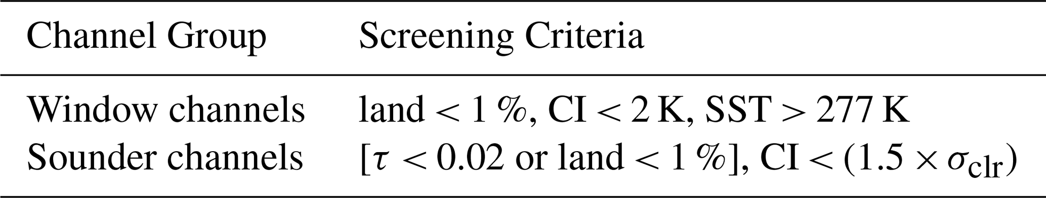
Lastly, other checks remove poorly modelled surface contributions, following quality control procedures used for all-sky assimilation. The checks screen out land, cold seas and sea-ice for window channels, as well as sounder channels with too much surface sensitivity over land (τ > 0.02). For window channels, screening of cold seas is driven by potential sea-ice and generally poor modelling of scenes over cold seas, both in terms of emissivity model biases and so-called “cold air outbreak” regions where the IFS struggles to produce sufficient cloud liquid water.

3.3.2 Screened data sample

The outcome of this screening can be seen in Fig. 4 for two AWS channels in a 12 h period. In the top panels, the full data sample of background departures is seen, with the cal/val screened sample shown in the bottom panels. The figure shows two sounding channels at different ends of the AWS frequency spectrum (53.596 and 325 ± 4.1 GHz), with quite different cloud sensitivity. The main biases relative to the model are fairly clear from even a few hours of data like this. Channel 18 exhibits little bias as a function of scan or location, whereas channel 4 has a cross-scan bias structure and slightly warm-biased observations at higher latitudes. Most of the larger cloud signals have been removed by the screening, but not all by any means. Most channel 4 scenes over land are removed, as the screening is conservative regarding surface sensitivity for sounding channels, though higher zenith angles at the scan edges typically make it past the screening due to low enough τ values.

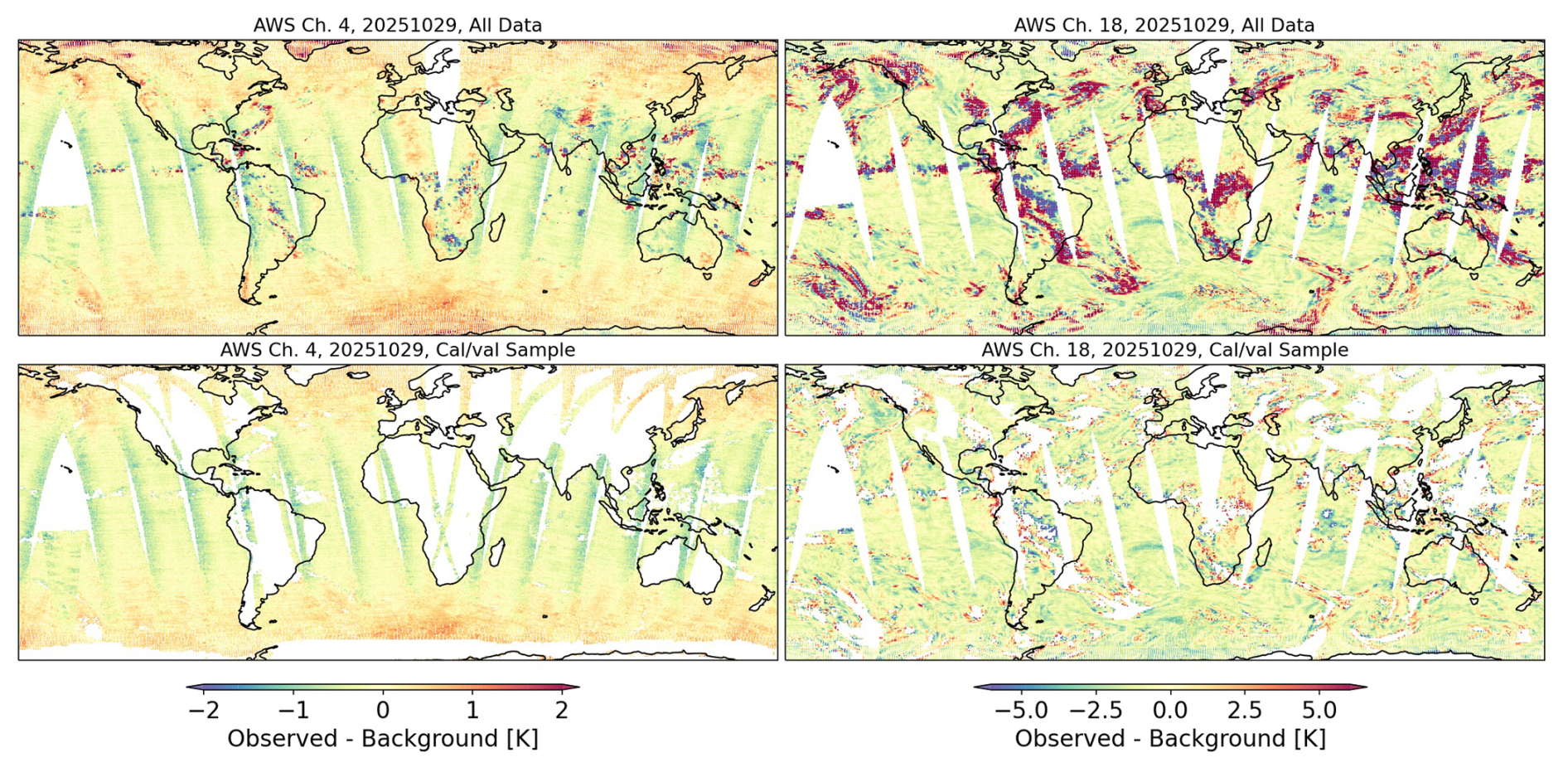
Figure 4 O–B from AWS channels 4 (left) and 18 (right) on 29 October 2025, showing the full data sample (top) and the cal/val sample after screening (bottom). No bias correction has been applied.

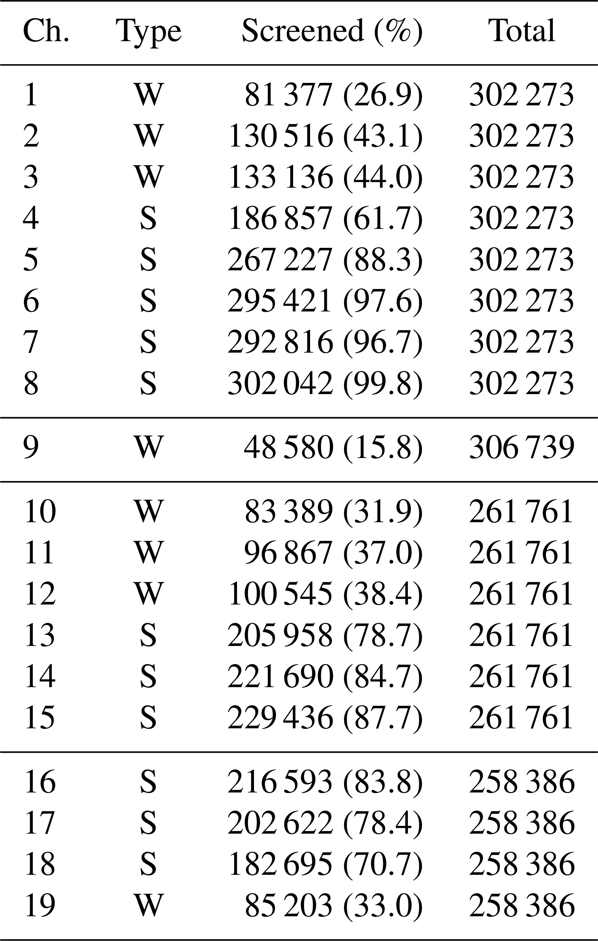
Using the same data, Table 3 illustrates how much of the total data remains after screening. Linked to the figure, 61.7 % and 70.7 % of the departures of the two channels shown are considered in the cal/val sample. The highest-peaking sounding channels (6–8) have very little data removed by the screening, and most of the true sounding channels witness 70 % of observations or more retained in the cal/val sample. The more surface- and cloud-sensitive window channels typically have 30 %–40 % of the data retained. 89 GHz is the most cloud-sensitive window channel, and this has the least data entering the cal/val sample. In this table we can also see the differing numbers of total superobs per feedhorn, driven by the swath overlap differences discussed earlier.

Table 3 Per channel, total data points (superobs) available in one 12 hr period on 29 October 2025, and those in the screened cal/val sample. Percentages of the total are given in parentheses. Channels are also defined as either window (W) or sounding (S) channels.

4 Results of radiometric performance assessment

Global biases relative to the IFS are given for all AWS channels in Fig. 5 for a 2-week period in autumn 2025, following the sampling strategy outlined above and using the assimilation system setup defined in the following section. For cross comparison, biases are also shown for multiple satellites carrying ATMS and MWHS-2 instruments, using the same sampling method. All AWS channels exhibit a mean bias against the IFS of about ±1 K or less. The sounding channel suites of AWS have relatively consistent biases within a given horn, with horns 1 and 3 slightly warmer than IFS, and horn 4 slightly cooler than IFS. Channel 14 is an outlier within horn 3, being about 0.5 K warmer than any other 183 GHz channel. Seen in the grey bars, a large majority of the total data available are retained in the cal/val sample for most channels.

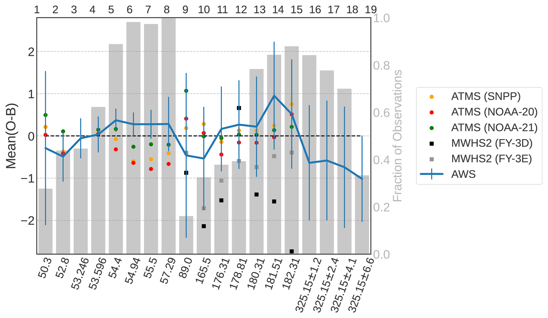
Figure 5 Global mean departures of AWS observations from cal/val sample, spanning 29 October to 12 November 2025. Equivalent channels (see Table 1) from ATMS and MWHS-2 are given by dots and squares, respectively, using the same sampling method. Blue vertical lines represent the standard deviation of departures within the cal/val sample for AWS, with grey bars showing the fraction of total observations in the sample. AWS channel numbers are given across the top, with corresponding frequencies across the bottom.

These global biases for AWS are comparable to the magnitudes seen for ATMS. As seen in the figure, most ATMS sounding channels are slightly cooler than IFS, but all are within ±0.75 K. MWHS-2 is also shown for comparison of 183 GHz suite biases, and its biases are typically larger in magnitude than those of AWS; FY-3E biases are generally more consistent and of smaller magnitudes than those of FY-3D (Steele et al., 2023). It is worth noting that mean biases relative to IFS do not preclude successful assimilation if VarBC is able to correct the biases adequately, but radiometric consistency within and between instruments is still valuable.

Along with global mean biases, the Gaussianity of departures is a good check of calibration quality, particularly for sounding channels, as skewed PDFs can point to bias structures such as orbital or scene temperature-dependent biases. Figure 6 shows the departure histograms for AWS data over sea from the same assimilation window seen in Fig. 4. This figure illustrates how much of the PDF “tails” are removed by the cal/val screening, more in line with the Gaussian curves shown in black. In most cases, the screening results in a more symmetric distribution of departures, for example by removing much of the positive tail seen for cloud-sensitive channels. The panels also illustrate how the cal/val sample mean can differ from that of the full data sample, particularly for the most cloud-sensitive channels (e.g. 9 and 19). The mode (as estimated by eye) appears to be almost identical in both samples, and typically very close to the mean of the screened sample, which also gives confidence in the screened sample mean providing a robust characterisation of the bias. In general, AWS departure histograms show relatively Gaussian behaviour for the sounding channels, indicative of limited or negligible structural biases on the global scale, and a general suitability for assimilation.

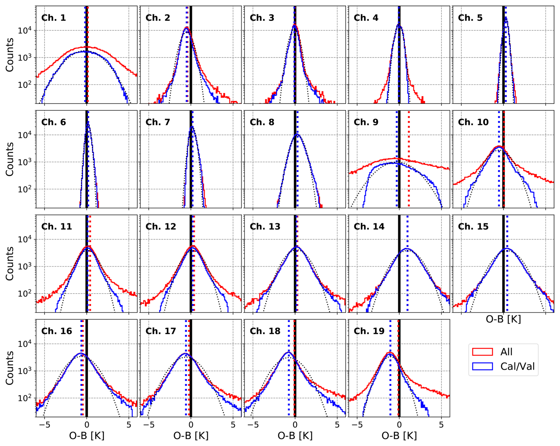
Figure 6 Histograms of AWS departures over ice-free oceans, 29 October 2025. Dashed vertical lines show the means of the full (red) and cal/val (blue) samples, respectively. A dotted black curve provides a Gaussian with mean and standard deviation of the cal/val sample for comparison.

Another important way to assess radiometric performance is to view biases as a function of scan position or zenith angle. This is a key test, as persistent biases at scan edges have been a limiting factor in assimilation of sounder radiances before, notably for AMSU-A and some channels on MWHS-2 (Duncan et al., 2022; Bormann et al., 2021). Figure 7 shows most of the purely sounding channels on AWS as a function of the scan position from feedhorn 1 (noting that scan positions between horns do not coincide, see Fig. 2). The feedhorn 1 channels exhibit relatively stable biases across-scan, but show slightly larger biases near scan edges. Especially for channel 7, the outer scan positions see a positive bias several tenths of a degree higher than the middle of the swath. The cause for this residual bias near scan edge for horn 1 is uncertain, but could be driven by insufficient spillover and near sidelobe corrections (Catalina Medina and Roland Albers, personal communication, 2026). Feedhorn 3 shows linearly increasing bias as a function of scan position, with the established cause of debris in the feedhorn (Eriksson et al., 2025). Feedhorn 4 displays very little bias that depends on scan position.

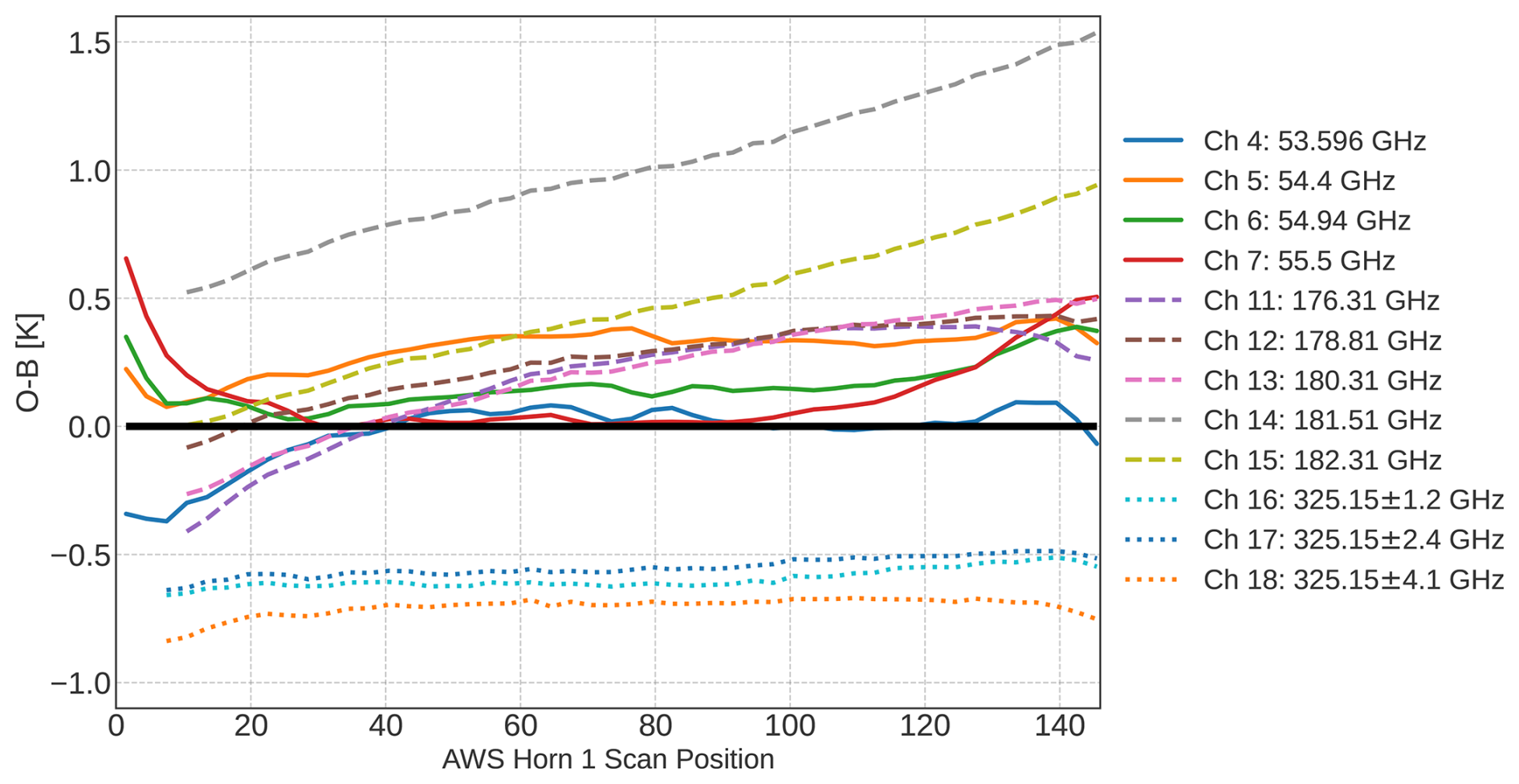
Figure 7 Cross-scan biases for assimilated channels, shown as a function of horn 1 scan positions. Global data from the screened cal/val sample, 29 October to 12 November 2025.

The magnitude of background errors is sufficiently small for temperature sounding channels (of order 0.1 K), that analysis of SD(O−B) is an effective way to assess NEDT. In contrast, humidity and cloud displacement errors in the background are typically an order of magnitude larger (1–2 K), and thus a similar analysis is not fruitful for establishing NEDT for window and humidity sounding channels. Hence we limit analysis of noise performance to feedhorn 1. Figure 8 shows SD(O−B) for the screened data sample, comparing AWS with equivalent channels from ATMS and AMSU-A on different platforms. AMSU-A shows nearly constant effective noise across the scan (as it is not superobbed in the IFS). For Metop-B and Metop-C AMSU-A, NEDT is mainly in the 0.15 to 0.20 K range for these tropospheric channels, though NEDT for some channels like Metop-C 5 and Metop-B 6 is now out of specification and significantly larger. AMSU-A channel 5, the lowest-peaking channel analysed here, shows a slight increase in SD(O−B) for low zenith angles, which is driven by larger background errors from greater cloud visibility near nadir rather than effective NEDT (Duncan et al., 2022). The same pattern is seen in ATMS channel 6 and AWS channel 4 for low zenith angles. ATMS observes out to higher zenith angles than AMSU-A, and we see a moderate increase in effective noise near scan edges where fewer observations make up a single superob. At the 50 km superob resolution, ATMS tropospheric channels achieve roughly 0.10 K noise near nadir, with slightly lower values seen for NOAA-20 (not shown) and NOAA-21 when compared to SNPP.

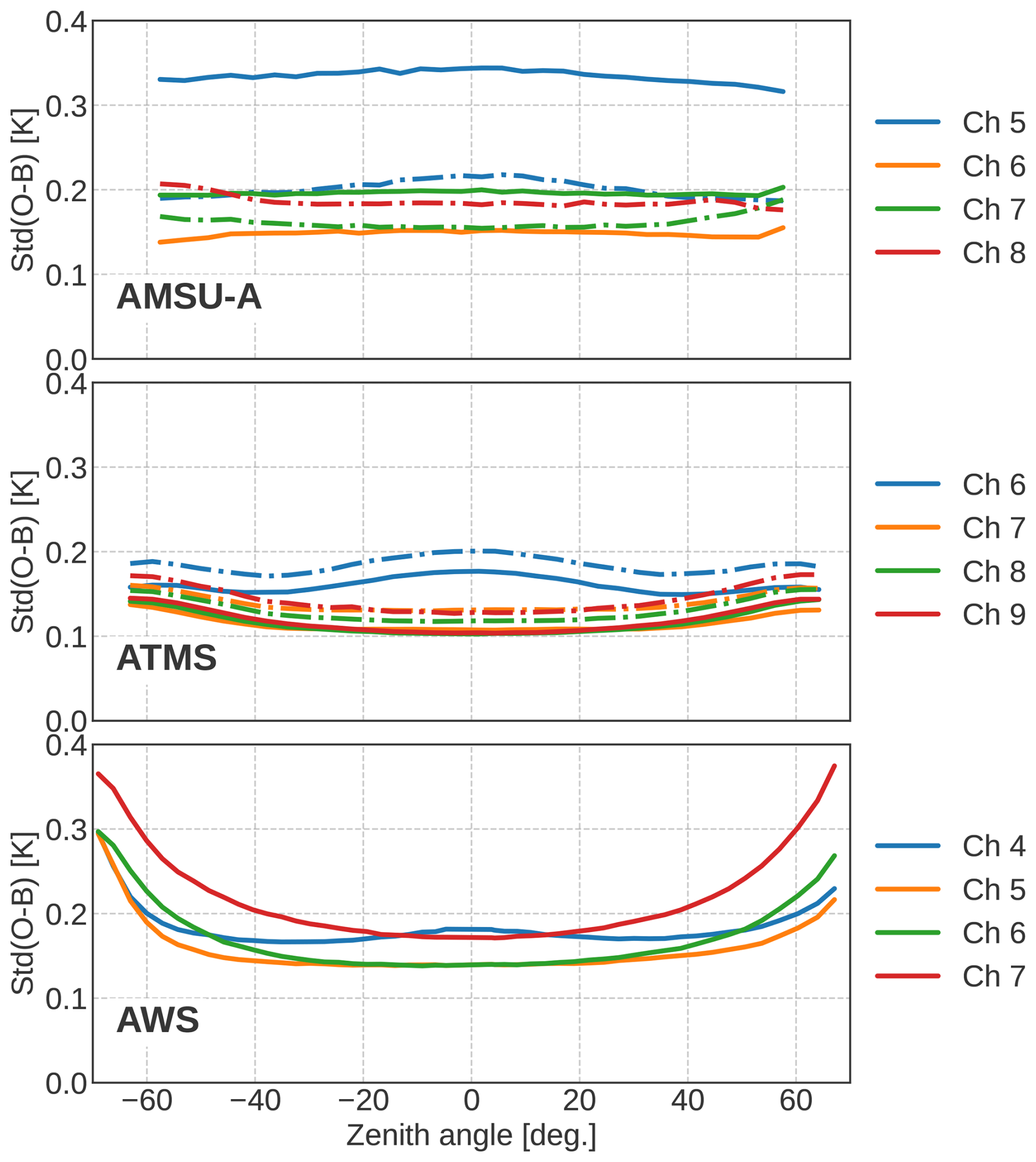
Figure 8 Standard deviations of background departures for AMSU-A (top), ATMS (middle) and AWS (bottom) as a function of zenith angle across the scan, after bias correction and for the cal/val screened sample. AMSU-A data are un-averaged whereas AWS and ATMS are superobbed to 50 km. For AMSU-A, Metop-C (solid) and Metop-B (dash-dot) are shown; for ATMS, SNPP (dash-dot) and NOAA-21 (solid) are shown.

AWS effective noise in the middle of the swath is comparable to that of AMSU-A and ATMS, with values of about 0.15 to 0.20 K SD(O−B) observed. Channel 5 is the best-performing for effective noise, achieving nearly ATMS level SD(O−B). Not shown is channel 8, which was known to be out of specification pre-launch (Eriksson et al., 2025), and even after superobbing does not fit on this plot. It is worth emphasising that outer scan positions of AWS observe at larger zenith angles than seen on heritage sounders, necessitating appropriate treatment of observation errors as discussed in Sect. 3.2.

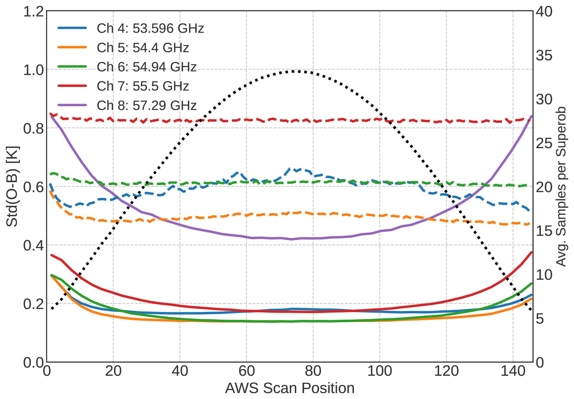
Figure 9 Standard deviations of background departures for AWS channel 4–8 with (solid) and without (dashed) superobbing. The mean number of observations per superob is given in the dotted black line. Data from 16–19 March 2025.

Lastly, while the noise performance for averaged data is what matters for assimilation, it is instructive to look at SD(O−B) for un-averaged radiances as well, because these values are closely tied to true sample NEDT of the instrument. Sample NEDT is the noise of individual observations, not to be confused with the footprint NEDT values given in Table 1 which represent averaging over the −3 dB FOV size (in the scan direction only); these can be quite different for heavily over-sampled instruments. Figure 9 shows results from a special experiment in which superobbing was switched off for AWS, comparing SD(O−B) for the same dates with and without superobbing. As un-averaged AWS data account for about 100 million observations per 12 hr assimilation window, this was run for only a few days. With the expanded y-axis, we can see the out of specification channel 8, and the un-averaged SD(O−B) values of about 0.48 to 0.82 for channels 4 to 7. This plot also shows the number of observations per average superob, peaking at over thirty near nadir and tailing off to fewer than ten for outer scan positions. For a purely white noise distribution, effective noise should decrease as a function of $\mathrm{1}/\sqrt{\left(N\right)}$ where N is observations per superob. As an example, channel 7 sample NEDT of 0.80 K with 30 observations per superob could achieve a maximum noise reduction to about 0.15 K, and this is close to what we observe. This analysis is also a check on the in-orbit NEDT values given by Eriksson et al. (2025), verifying that channels 4 to 7 are indeed within the specified NEDT of 0.4 K for the −3 dB sample (see Duncan et al., 2025a for details).

A final point worth emphasising is that calibration for most AWS channels has changed since launch, with several updates made to the level 1 processing. Most of the analysis of radiometric performance in this paper focuses on data after a key calibration update by ESA in late October 2025, whereas the assimilation trials were performed over an earlier period before this update, January through September of 2025. A previous report (Duncan et al., 2025a) analysed these earlier level 1 data, and some global biases have significantly improved since then. There is thus potential for AWS calibration to improve further in the future. Temporal stability of AWS radiances is not addressed here, but time series of AWS departures are publicly available from ECMWF monitoring pages (https://charts.ecmwf.int/catalogue/packages/obstat/, last access: 28 May 2026).

5 Assimilation results

The results herein use IFS model cycle 49r1, the operational ECMWF model version as of early 2026 (ECMWF, 2024). Experiments were run at Tco399 (27 km) horizontal resolution with 137 vertical levels. The data assimilation uses incremental 4D-Var with three outer loops and a final inner-loop resolution of 80 km, with flow-dependent background error covariances coming from the operational ensemble of data assimilations (EDA). Two 12 h long-window assimilation cycles are run daily, spanning windows from 09:00–21:00 and 21:00–09:00 UTC. Other than AWS, the remainder of the global observing system is unchanged from that used operationally for those dates, including other MW instruments like AMSU-A and ATMS.

Two observing system experiments (OSEs) are compared, covering nine months from January to September, 2025. In the control, observations are assimilated just as in ECMWF operations; in the AWS experiment, assimilation of AWS is added. As presented in Sect. 3.2, actively assimilated channels include 4–7 and 11–18. These are equivalent frequencies to ATMS 6–9 and 18–22, plus three of the four sub-mm channels on AWS. AWS radiances are assimilated over both land and sea with limited exceptions for sea-ice, frozen surfaces, and high orography, depending on the frequency (see Table 3 in Geer et al., 2022). The full swath width of feedhorns 3 and 4 is assimilated; due to residual biases at outer scan positions after VarBC is applied, outer scan positions from feedhorn 1 (zenith angles 62° and greater) are not assimilated.

5.1 Impact on short-range forecasts

Short-range forecast impact can be judged by changes in background fits to independent observations. Figure 10 shows the normalised change in SD(O−B) for six different observation types spanning temperature, humidity, and wind measurements. The 100 % line represents the control experiment (i.e. without AWS assimilated), so points below this indicate an improved fit between the observations and the model background after adding AWS to the assimilation, i.e. an improved short-range forecast. AWS clearly improves the short-range forecasts of humidity, with decreased SD(O−B) seen for ATMS humidity channels 18–22, several of IASI's humidity-sensitive wavenumbers of 1367 to 1994, and water vapour channels from GOES-18 and Meteosat-9, though radiosonde humidity fits appear largely neutral. There are also some small but significant improvements in fits to wind observations in the upper troposphere, seen in panel (c). The impact on short-range temperature forecasts is relatively small, with an overall neutral change seen in hyperspectral infrared instruments like IASI but some slight improvements seen for radiosonde temperature in the mid troposphere and ATMS channels 6–9.

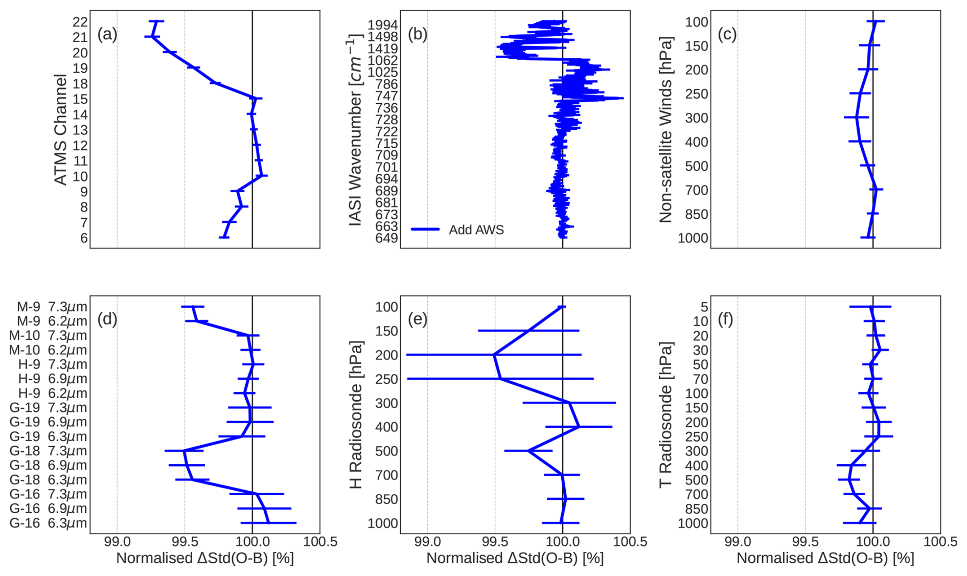
Figure 10 Global changes in SD(O−B) for independent observations from ATMS (a), IASI (b), non-satellite winds (c), geostationary infrared radiances (d), humidity (e) and temperature (f) radiosondes. Confidence intervals for 95 % statistical significance are given in horizontal bars. In panel (d), M, H, and G represent Meteosat, Himawari, and GOES, respectively.

Not every signal in Fig. 10 is positive, but this picture is generally consistent with activations of MW sounders from heritage platforms in the IFS (e.g. Steele et al., 2023). Due to the large number of humidity-sensitive channels on AWS (five at 183 GHz plus three active at 325 GHz), it is not surprising that the main impact from AWS is on humidity. An interesting feature here is that fits to GOES-18 and Meteosat-9 are quite significantly improved but impacts are neutral for the others in the “geo ring”. This is linked to strong improvements in background fits to observations in two distinct longitude bands near 45° E and 135° W. This appears to be linked to the orbital crossing time of AWS (10:30 LT), filling in a gap between other sounder overpasses (see Fig. 1). AWS provides extra constraint for humidity late in the 12 h assimilation window for these longitude bands, which has a larger impact on the forecast in a well-documented effect (McNally, 2019). It is a timeslot that otherwise has limited MW data at these longitude bands (being about 1 h after Metop-B and -C), and this manifests in improved fits to GOES-18 and Metosat-9 infrared radiances once AWS is added.

5.2 Impact in medium range

To analyse the medium-range impact we examine analysis-based forecast verification. Statistical significance testing of medium-range forecast impacts follow Geer (2016), with 95 % confidence levels given. Forecast impacts are gauged by forecast error reduction in reference to the control, with negative values signifying less error in the experiment and thus a positive impact on the forecast from assimilation of AWS.

Figure 11 presents the changes in RMSE for winds at two levels (850 and 200 hPa) and geopotential height at 500 hPa, spanning forecast lead times of 2 to 7 d. Significant improvements in forecast skill can be seen in the Southern Hemisphere through day 4, with relatively neutral impacts seen in the tropics and Northern Hemisphere. This is roughly in line with the impacts seen from adding another MWHS-2 into the IFS (Steele et al., 2023), but with a slightly larger impact on temperature. This indicates that AWS is able to positively affect medium-range forecast skill in a similar way as heritage MW sounders assimilated in the IFS.

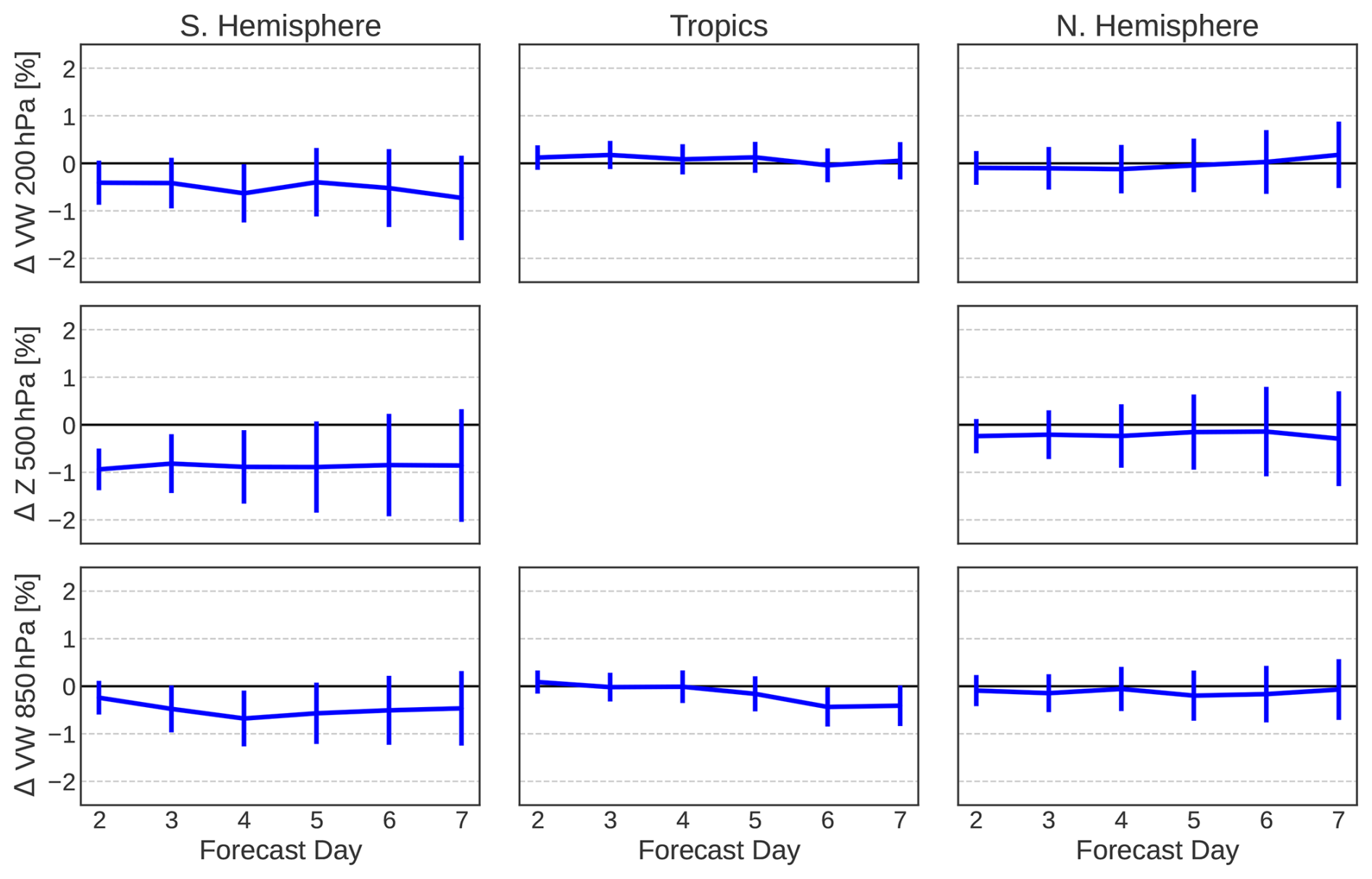
Figure 11 Changes in RMSE for forecast scores at day 2 to 7 caused by assimilation of AWS. Shown are vector wind at 200 hPa (VW; top), geopotential height at 500 hPa (Z; middle), and vector wind at 850 hPa (bottom) for the Southern Hemisphere (90 to 20° S), Tropics (20° S to 20° N), and Northern Hemisphere (20 to 90° N). Geopotential scores in the Tropics are not informative and hence not included.

To visualise the spatial distribution of these impacts, Fig. 12 shows the normalised change in RMSE for winds at four forecast lead times. These plots indicate that the majority of the forecast improvements from AWS are seen at high latitudes in both hemispheres. From the free troposphere down to the surface, winds are improved by about 1 % to 3 % at short-range near the poles and some of this signal lasts through to day 4 forecasts. Similar signals are witnessed in verification of humidity forecasts (not shown).

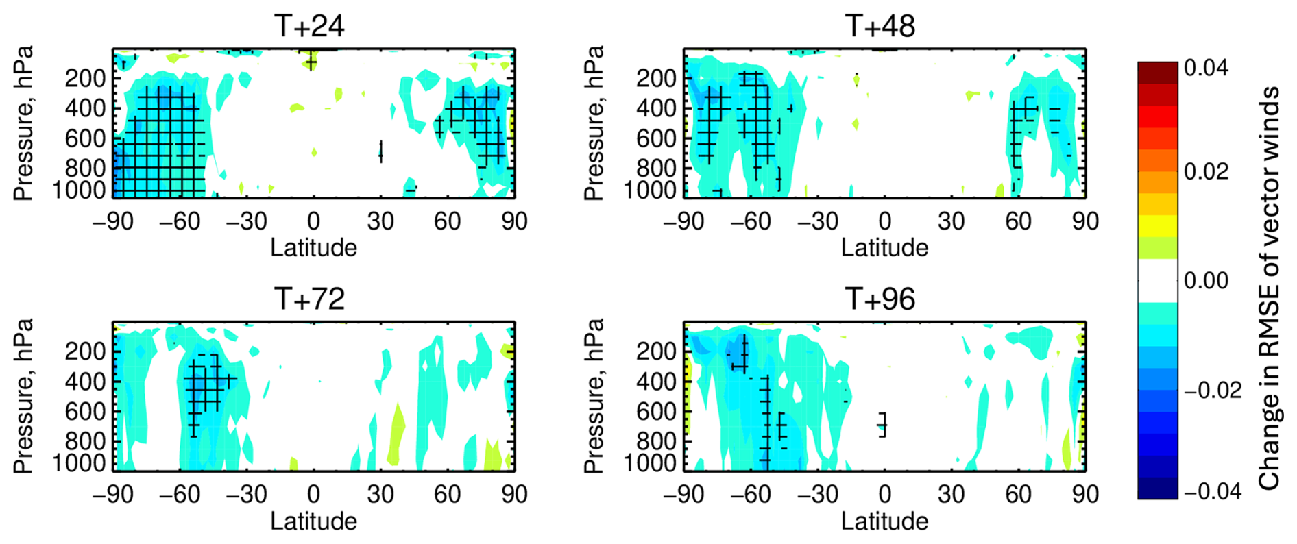
Figure 12 Change in vector wind RMSE when adding AWS to the assimilation, normalised by the standard deviation of the control RMSE. Verification is given at 24, 48, 72, and 96 h forecast lead time. Hatching shows statistical significance at the 95 % confidence level. Here the verification reference is the operational analysis to avoid own-analysis artefacts at 24 h.

5.3 Forecast sensitivity to observation impact (FSOI)

Another way to characterise the influence of assimilated observations in NWP is through the adjoint-based Forecast Sensitivity to Observation Impact (FSOI). The FSOI metric estimates whether each observation reduced or increased forecast errors at a 24 h lead time based on analysis verification with respect to a dry total energy norm (Cardinali, 2009). Here we will use FSOI from the operational system, which uses 12 h assimilation windows as before but runs at 9 km horizontal resolution with a final inner-loop resolution of 40 km. AWS has been assimilated operationally since 10 July 2025, and the statistics here run from this date through October 2025. Note that FSOI statistics give only broad estimates of short-range forecast impacts of contributing observations in the presence of the full observing system used, and limitations of FSOI and its complementarity to OSEs are further discussed by Healy et al. (2024).

The geographic distribution of total FSOI for AWS channel groups 4–7, 11–15, and 16–18 is shown in Fig. 13. As discussed above, the main impact of AWS assimilation is felt in distinct longitude bands that correspond to the last hours of the 12 h assimilation window observed by AWS with its 10:30 orbital crossing time (see Fig. 1). In terms of relative magnitudes, the 183 GHz channels are the most impactful set, followed by the 50 GHz temperature sounding channels. The 325 GHz channels do provide positive impact, most notably in regions near Antarctica, but less in aggregate than the 183 GHz suite. Though FSOI can be a noisy diagnostic especially on short timescales, it is interesting that some regions exhibit what appears to be sustained negative impact. For instance, temperature sounding channels off the Horn of Africa and the 183 GHz suite east of Asia show some small but non-negligible degradation in FSOI. These seem to coincide with areas of known SST biases, and warrant further investigation.

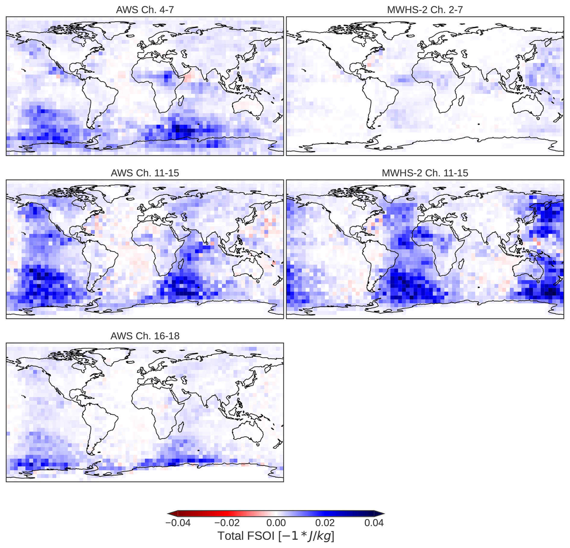
Figure 13 Total FSOI on a 5° grid for AWS (left) and FY-3E MWHS-2 (right) from ECMWF operations, 10 July to 7 October 2025. Channels from AWS and MWHS-2 are grouped by temperature sounding (top), 183 GHz (middle), and 325 GHz for AWS (bottom). Note that “good” FSOI is typically negative but the sign has been changed here to aid interpretation.

Alongside the total FSOI maps for AWS channel groups, Fig. 13 also shows MWHS-2 from FY-3E. As FY-3E flies in a sparsely sampled orbit (05:30 or “early morning”), and MWHS-2 has five equivalent 183 GHz channels, it provides a useful point of comparison. Following AWS, the channels of MWHS-2 are grouped, now with 118 GHz temperature sounding channels (2–7) and 183 GHz humidity channels (11–15) shown together. The total FSOI patterns for FY-3E MWHS-2 are remarkably similar to AWS for the 183 GHz suite, albeit shifted as expected from the different equator crossing time, with large impacts in the Southern Ocean especially. FY-3E also shows the clear signal of impacts maximising in two longitude bands, again linked with timeslots late in the 12 h assimilation windows (compare with Fig. 1). The FSOI results thus back up the background fits to geostationary infrared radiances (Fig. 10), linking impact to orbital crossing time. Lastly, if we compare the impact for MWHS-2 118 GHz channels with those of AWS 50 GHz channels, it is clear that the 50 GHz suite is more impactful. This is especially the case in the persistently cloudy Southern Ocean, where the 50 GHz suite penetrates clouds better than at 118 GHz, which is much more sensitive to attenuation from cloud and precipitation. In addition, the 50 GHz suite typically displays lower sensor noise than 118 GHz, which is crucial for temperature increments.

In late 2025, AWS and FY-3E MWHS-2 are typically two of the most impactful satellite instruments assimilated in the IFS as judged by FSOI. The large FSOI totals seem largely driven by the unique orbital crossing times of these two satellites. It is also clear that AWS achieves significant impact from each suite of sounding channels, though the sub-mm suite is currently the least impactful of the three. As this is the first time that sub-mm channels are assimilated in global NWP, there is surely scope for refinement, and these achieved contributions are already very encouraging.

6 Conclusions

This paper has presented two main analyses. First was an assessment of AWS instrument performance through the lens of an NWP system. Second was presentation of the results of assimilating AWS in an all-sky framework in the ECMWF data assimilation system. These two halves complement each other, as poor radiative performance would have precluded successful assimilation of AWS, and we should thus discuss them in order.

The all-sky NWP method of calibration/validation analysis described herein allowed rapid assessment of AWS radiances early in the mission lifetime. With the NWP fields serving as a reference, double differences with heritage instruments are readily analysed by employing the same sampling criteria, with millions of comparisons available daily to quickly accrue a large statistical sample. Comparisons were made to operationally assimilated sounders ATMS, AMSU-A, and MWHS-2.

AWS calibration biases are within 1.0 K of the IFS reference globally. Some channels on feedhorn 1 exhibit more complex biases near the scan edge, with unclear mechanisms at play. The high zenith angles observed by AWS are also a challenge for the forward model, but given the channel-specific nature of these bias structures, it appears to be a calibration issue on feedhorn 1. Some aspects of the antenna pattern characterisation may warrant further consideration to remove these biases at source. The 183 GHz channels on feedhorn 3 show a linear cross-scan bias that has been documented by Eriksson et al. (2025) as likely due to debris in the feedhorn from the shared launch. In contrast, the novel 325 GHz channels exhibit effectively no bias concerns and have been consistently close to the IFS reference since the earliest data available. Effective noise levels for feedhorn 1 channels are comparable to AMSU-A after spatial averaging but typically higher than equivalent ATMS channels treated the same way. The NWP analysis of un-averaged sample noise corroborates reported in-orbit NEDT estimates from Eriksson et al. (2025) and shows that most channel noise estimates are within specifications.

Given the quality of AWS radiometric performance, assimilation trials were performed. AWS has shown a significant, positive impact on forecast skill over a 9-month period of experimentation. This manifested as improved short-range forecasts of winds and humidity as seen in background fits to independent observations, as well as medium-range impact judged by analysis-based verification. Winds at upper and lower levels in the Southern Hemisphere are improved through forecast day 4. AWS also performs well when quantified by the adjoint-based FSOI. Here we have linked this to the orbital crossing time of AWS, contrasted with that of FY-3E, whilst noting that FSOI magnitudes do not translate directly to medium-range impact. The novel 325 GHz channels are the first sub-mm radiances assimilated operationally in global NWP. This new frequency band shows positive impact in the IFS, but is not as impactful as the 183 GHz suite; here only FSOI has been shown to analyse 325 GHz suite impact, whereas an OSE analysis has been performed previously (Duncan et al., 2025a). Work is ongoing to better understand the physical mechanisms underlying sub-mm assimilation impacts in 4D-Var.

AWS assimilation was previously assessed over a shorter time period and against a depleted observing system that anticipated the loss of the legacy satellites NOAA-15, -18, and -19 (Duncan et al., 2025a). These platforms constituted four sounders assimilated at ECMWF (three AMSU-A instruments and one MHS), with NOAA-15 AMSU-A a mainstay of the global observing system since the late 1990s; they were all decommissioned in June 2025, in the middle of the time period analysed here. The addition of AWS to the ECMWF operational assimilation in July 2025 thus helped fill a gap for sounding left by the decommissioning of these legacy platforms. The positive results here contained NOAA-15, -18, and -19 sounders for a majority of the time period analysed, and the forecast impact of AWS addition remained positive both before and after June 2025 (not shown).

Further work will be needed to maximise the total forecast impact of AWS assimilation. Future work should include optimising the assimilation strategy for 325 GHz channels, especially how this channel suite can complement the well-known 183 GHz suite in various atmospheric conditions. Surface emissivity modelling is also of interest in this band, as sufficient characterisation of the surface contributions to measured radiances could unlock assimilation over places like Greenland and Antarctica that are typically dry aloft but with significant cloud amounts present near the surface. Lastly, the lower-peaking temperature sounding channels have not been assimilated here (AWS channels 2 and 3), but should be considered in the future.

AWS has proven that a small-satellite MW radiometer can achieve radiometric performance sufficient for assimilation in operational NWP; the even smaller CubeSat class of satellites have not yet proven this level of data quality. However, this area of satellite meteorology is rapidly evolving. Part of the rationale for EPS-Sterna is to place sounders in between the three baseline orbits covered by NOAA, EUMETSAT, and CMA. The results presented here demonstrate that there is significant benefit to global NWP from placing a high-quality sounder at a different orbital crossing time. The results have also shown benefit from assimilation of sub-mm radiances, which bodes well for future instruments with sub-mm channels such as ICI. Assuming that more AWS-style radiometers are launched, the future is bright for achieving even greater forecast improvements from microwave sounder assimilation.