Processing multiple GNSS RO data using FSI and ROPP: results from the ROMEX

Global Navigation Satellite System (GNSS) Radio Occultation (RO) is a vital technique in atmospheric remote sensing, providing all-weather, high-resolution vertical observations that support numerical weather prediction (NWP) and atmospheric research. To enhance understanding of GNSS RO processing uncertainties and inter-algorithm consistency, NOAA/STAR developed an independent RO inversion algorithm based on the Full Spectrum Inversion (FSI) technique to derive bending angle and refractivity profiles from excess phase data. As part of the international Radio Occultation Modeling Experiment (ROMEX), endorsed by the International Radio Occultation Working Group (IROWG), STAR's FSI results were systematically compared with outputs from the community standard Radio Occultation Processing Package (ROPP) and EUMETSAT datasets. Leveraging multi-GNSS RO observations from both commercial and government-funded missions, the study evaluates consistency across processing approaches using the European Centre for Medium-Range Weather Forecasts (ECMWF) Reanalysis v5 (ERA5) as the reference and structural differences against the three-dataset mean for the ROMEX period. Results reveal high overall agreement, while identifying variations linked to the signal-to-noise ratio (SNR) and mission characteristics, providing critical insights for interpreting ROMEX forecast impact studies and improving GNSS RO data assimilation systems.

1 Introduction

Global Navigation Satellite System (GNSS) Radio Occultation (RO) has become a cornerstone of atmospheric remote sensing, offering high vertical resolution, global coverage, long-term stability, and minimal bias (Kursinski et al., 1997; Anthes et al., 2008; Ho et al., 2020). By measuring the bending of GNSS signals as they pass through the atmosphere, RO enables retrievals of refractivity, temperature, pressure, and humidity profiles. As a limb-sounding technique, it is largely unaffected by clouds and precipitation, providing an all-weather observing capability essential for weather forecasting and climate monitoring (Cucurull et al., 2007; Healy, 2008; Steiner et al., 2020).

Over the past two decades, the expansion of GNSS constellations (e.g., GPS, GLONASS, Galileo, BeiDou) and the increasing availability of RO missions, including government-funded programs (e.g., COSMIC-1/2, Metop-A/B/C, Sentinel-6) and commercial ventures (e.g., Spire, GeoOptics, PlanetiQ), have significantly increased the volume of RO observations (Anthes, 2011; Schreiner et al., 2020; Ho et al., 2023). Today, global RO data counts exceed 35 000–40 000 profiles per day, with substantial contributions from commercial providers through initiatives such as NOAA's Commercial Data Purchase (CDP) program. While this growth enhances the value of RO for numerical weather prediction (NWP) and climate applications, it also introduces challenges due to differences in instrument design, tracking strategies, sampling patterns, and processing methodologies.

RO retrievals involve several steps: (i) deriving clock-synchronized excess phase and signal-to-noise ratio (SNR) data, (ii) inverting excess phase to bending angle (BA) profiles, and (iii) retrieving refractivity from BA via Abel or statistical methods (Gorbunov, 2002a, b). In the lower troposphere, strong gradients and multipath propagation complicate retrievals, motivating advanced inversion techniques such as Full Spectrum Inversion (FSI) (Jensen et al., 2003; Adhikari et al., 2016, 2021), Canonical Transform Type 2 (CT2) (Gorbunov et al., 2005), and Phase Matching (PM) (Jensen et al., 2004; Sokolovskiy et al., 2010). FSI relies on explicit signal localization to enhance vertical resolution and mitigate multipath by reducing spectral mixing, whereas CT2 achieves an implicit, physics-based localization in impact parameter space, enabling more robust separation of multipath contributions. While FSI is designed to leverage full-spectrum information for potentially enhanced sensitivity to fine-scale atmospheric structures, it is also generally more noise-sensitive. CT2, in contrast, provides more stable retrievals in strong multipath conditions, sometimes at the expense of reduced small-scale resolution. Consequently, the effective vertical resolution of both methods is highly dependent on specific implementation and tuning choices, such as filter settings and truncation strategies.

The international RO community is currently undertaking a coordinated effort to evaluate the impact of large volumes of RO data on NWP. This initiative, known as the Radio Occultation Modeling Experiment (ROMEX), is endorsed by the International Radio Occultation Working Group (IROWG) (https://irowg.org/ro-modeling-experiment-romex/, last access: 27 May 2026) and provides a collaborative platform for data providers and processing centers to assess RO retrievals under a standardized framework (Anthes et al., 2024). GNSS RO observations from a broad range of government-funded and commercial missions were submitted to EUMETSAT for centralized processing, and the resulting products were distributed via the Radio Occultation Meteorology Satellite Application Facility (ROM SAF). ROMEX provides a standardized framework for assessing inter-mission and inter-algorithm differences. Central questions include whether assimilating larger RO volumes improves forecasts, and how variations in data quality and inversion methods affect the outcome.

In support of ROMEX, the NOAA Center for Satellite Applications and Research (STAR) contributed independent datasets processed using the FSI algorithm (RFSI), which was integrated into version 10.0 of the Radio Occultation Processing Package (ROPP) (Culverwell, 2020). This customized system, hereafter referred to as STAR ROPP, retains compliance with ROPP standards while incorporating STAR-developed retrieval capability, including both the CT2 and FSI methods for bending angle retrieval. Here, STAR RFSI denotes the STAR implementation of the FSI-based bending angle retrieval, while STAR ROPP refers to the customized ROPP v10.0 framework developed at STAR that supports both CT2 and FSI processing. This system is distinct from the official ROM SAF ROPP, which serves as the community standard. In this study, the community-standard dataset refers specifically to data generated using the STAR ROPP CT2 method. Maintaining this distinction is essential, as it enables an independent assessment of algorithmic effects on RO data quality.

FSI offers a specific approach for resolving fine-scale atmospheric structures and handling multipath in the lower troposphere (Jensen et al., 2003; Adhikari et al., 2021), a key source of uncertainty for NWP. The use of the STAR RFSI algorithm within ROMEX is therefore to quantify the structural uncertainty associated with this alternative retrieval approach, which is sensitive to small-scale features, relative to community-standard methods, thereby providing critical insight for optimizing multi-mission data assimilation strategies.

This study evaluates the STAR FSI-based processing system within the ROMEX framework. Retrievals from RFSI are compared against those from the STAR ROPP with the CT2 method and the EUMETSAT-processed ROMEX dataset (with COSMIC-2 data provided by UCAR). The analysis focuses on November 2022 and utilizes the European Centre for Medium-Range Weather Forecasts (ECMWF) Reanalysis v5 (ERA5) (Hersbach et al., 2023) as a reference to evaluate algorithmic performance across various missions. The STAR RFSI dataset for ROMEX is one of the three RO datasets, along with those from EUMETSAT and UCAR, that were released to ROMEX participants through ROM-SAF (Shao and Folsche, 2024).

Intercomparisons included statistical evaluations (mean biases, standard deviations) and inter-algorithm consistency. This design helps isolate processing-related uncertainties (e.g., structural uncertainty; Ho et al., 2012) and ensures that differences in NWP impact can be attributed to data quality and processing methodology rather than uncontrolled input or evaluation effects.

The paper is organized as follows: Sect. 2 describes the GNSS RO observations and datasets used in this study. Section 3 presents the FSI algorithm in detail. Section 4 provides inter-algorithm and inter-mission comparison results using ROMEX RO data. Conclusions are summarized in Sect. 5.

2 GNSS RO Observations and Data Used in this Study

2.1 GNSS RO Observations

Modern satellite missions, including COSMIC-2, Spire, and PlanetiQ, have significantly increased the volume of GNSS radio occultation data. These missions track signals from multiple constellations, including GPS, GLONASS, Galileo, and BeiDou, thereby improving global spatial and temporal coverage for atmospheric profiling.

Table 1 RO Missions are included in ROMEX.

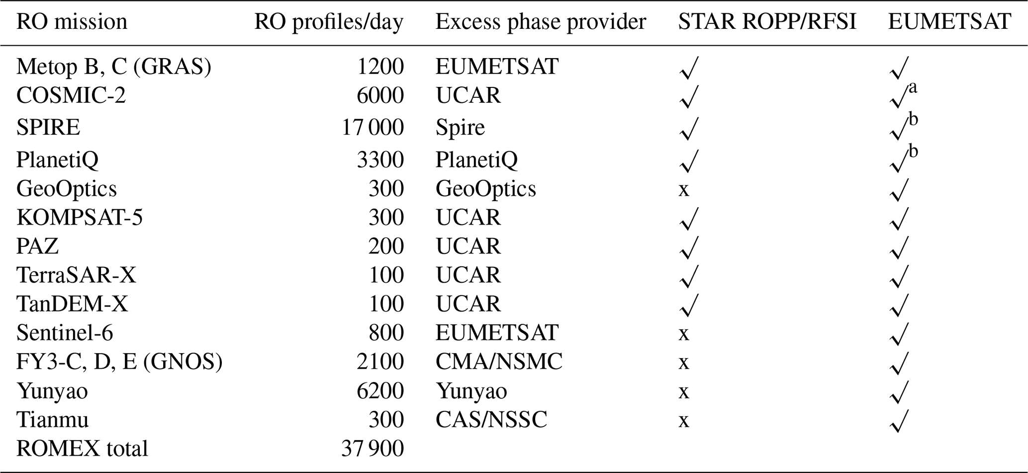
^∗ UCAR provided both bending angle and refractivity in the EUMETSAT ROMEX dataset. ^b No refractivity available in the EUMETSAT dataset for PlanetiQ and Spire, only bending angle.

LEO satellite receivers track GNSS signals using two primary methods: Closed Loop (CL) and Open Loop (OL). CL tracking ensures stable signal acquisition in the upper atmosphere but may fail under rapidly varying conditions in the lower troposphere. OL tracking, by contrast, is specifically designed to capture multipath-affected signals in the lower atmosphere. The combination use of CL and OL tracking was traditionally adopted to ensure reliable performance across the full vertical extent of the atmosphere. However, recent GNSS radio occultation missions, including COSMIC-2, Spire, and PlanetiQ, primarily employ OL tracking throughout the occultation in order to maximize tracking robustness and data continuity across all atmospheric layers.

The raw data, consisting of signal phase and amplitude measurements, are processed to calculate bending angle and refractivity profiles. A critical step in this process is correcting ionospheric effects. This is achieved by using dual-frequency signals (e.g., L1 and L2), which allow separation of the frequency-dependent ionospheric interference from the non-dispersive signal of the neutral atmosphere. This isolation is essential for accurate atmospheric retrievals.

2.2 RO Data Used in this Study

This study utilizes Level 1b atmospheric excess phase data (in conPhs/atmPhs format) from the ROMEX campaign. The dataset includes contributions from commercial providers, such as PlanetiQ, Spire, and GeoOptics, as well as government-funded missions, including Metop-B/C and COSMIC-2. A summary of mission-specific data coverage for the period 1 September to 30 November 2022 is provided in Table 1. These excess phase datasets, delivered in NetCDF format and available exclusively to ROMEX participants, serve as the primary input for deriving neutral atmospheric bending angle and refractivity profiles. On average, the dataset comprises approximately 37 900 profiles per day.

The high scientific value and cost-effectiveness of GNSS RO technology have driven increased private-sector participation in recent years. US companies Spire Global, PlanetiQ, and GeoOptics, along with Yunyao Aerospace in China, have deployed RO receivers on commercial satellites to supply high-quality data to the scientific community. Among them, Spire Global Inc. contributes approximately 17 000 profiles per day to ROMEX, followed by Yunyao Aerospace with about 6200, PlanetiQ with about 3300, and GeoOptics with roughly 300.

Several government-funded RO satellite missions were routinely processed by the UCAR COSMIC Data Analysis and Archive Center (CDAAC) and made available to both the research and operational communities during the ROMEX period. These missions include COSMIC-2 (∼ 6 000 profiles/day), KOMPSAT-5 (∼ 300), PAZ (∼ 200), and both TerraSAR-X and TanDEM-X (∼ 100 each). RO data from Metop-B/C and Sentinel-6 were provided by EUMETSAT, delivering approximately 1200 and 800 profiles per day, respectively. RO profiles from FY-3C/D/E and Tianmu were supplied by the National Satellite Meteorological Center (NSMC) of the Chinese Meteorological Administration (CMA) and the National Space Science Center (NSSC) of the Chinese Academy of Sciences (CAS), respectively, with average daily counts of approximately 2100 and 300.

For this study, we processed RO data from all ROMEX missions except Sentinel-6 and GeoOptics, as well as from the Chinese government or Chinese companies (e.g., FY-3, Yunyao, and Tianmu). For each processed mission, we generated bending angle and refractivity profiles using both the STAR RFSI and STAR ROPP (CT2) algorithms. These datasets were submitted to EUMETSAT and distributed to ROMEX participants through the ROM SAF. By processing multiple missions with independent algorithms, we ensured consistent inputs across platforms. We enabled a direct assessment of algorithm-dependent uncertainties, thereby clarifying how data processing influences the interpretation of ROMEX NWP impact experiments. Table 2 summarizes the typical SNR characteristics of GNSS receivers across different missions, supporting the discussion of mission-dependent performance and structural uncertainties.

Table 2 Signal-to-Noise Ratio (SNR)^∗ characteristics of GNSS receivers across different missions.

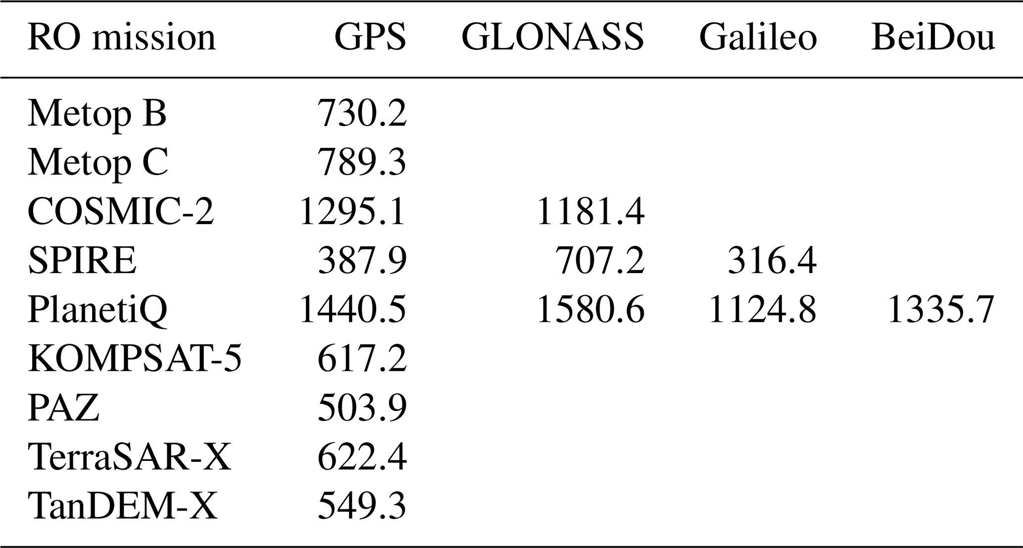
^∗ Mean SNR between altitudes 60 and 80 km, with unit (volt/volt).

3 Full Spectrum Inversion Algorithm and Processing Chain

The core FSI algorithm remains consistent with that described in Adhikari et al. (2021). The novelty of the present work is not in the invention of the FSI algorithm, but in the successful development and systematic application of the complete STAR RFSI end-to-end processing framework and its subsequent inclusion in the ROMEX intercomparison as an independent data source.

The scientific contribution is distinct from previous FSI work in three key ways. (1) Systematic Multi-Mission Application: This study provides the first comprehensive, cross-mission validation of the STAR RFSI system using a large and diverse ROMEX dataset (including commercial and government-funded missions) against other major community processing centers (such as EUMETSAT and UCAR). (2) Quantification of Structural Uncertainty: The primary objective and scientific value of this study is the quantification of the structural uncertainty among different processing approaches, FSI, STAR CT2, and the EUMETSAT ROM SAF ROPP CT2, under a ROMEX framework. This analysis provides critical metrics for interpreting ROMEX forecast impact studies. (3) Operational Documentation: The manuscript documents the complete STAR RFSI processing chain (including data preprocessing, quality control, and statistical optimization), which is essential for transparency and future operational use within NOAA STAR. The STAR RFSI algorithm provides a robust framework for generating bending-angle and refractivity profiles from GNSS RO measurements, particularly in the presence of lower-tropospheric multipath. As described by Chen et al. (2024), the STAR RFSI algorithm has been integrated into ROPP version 10.0 customized at NOAA STAR. RFSI processes dual-frequency excess phase and SNR data along with satellite position and timing information. It supports a wide range of satellite missions and tracking configurations.

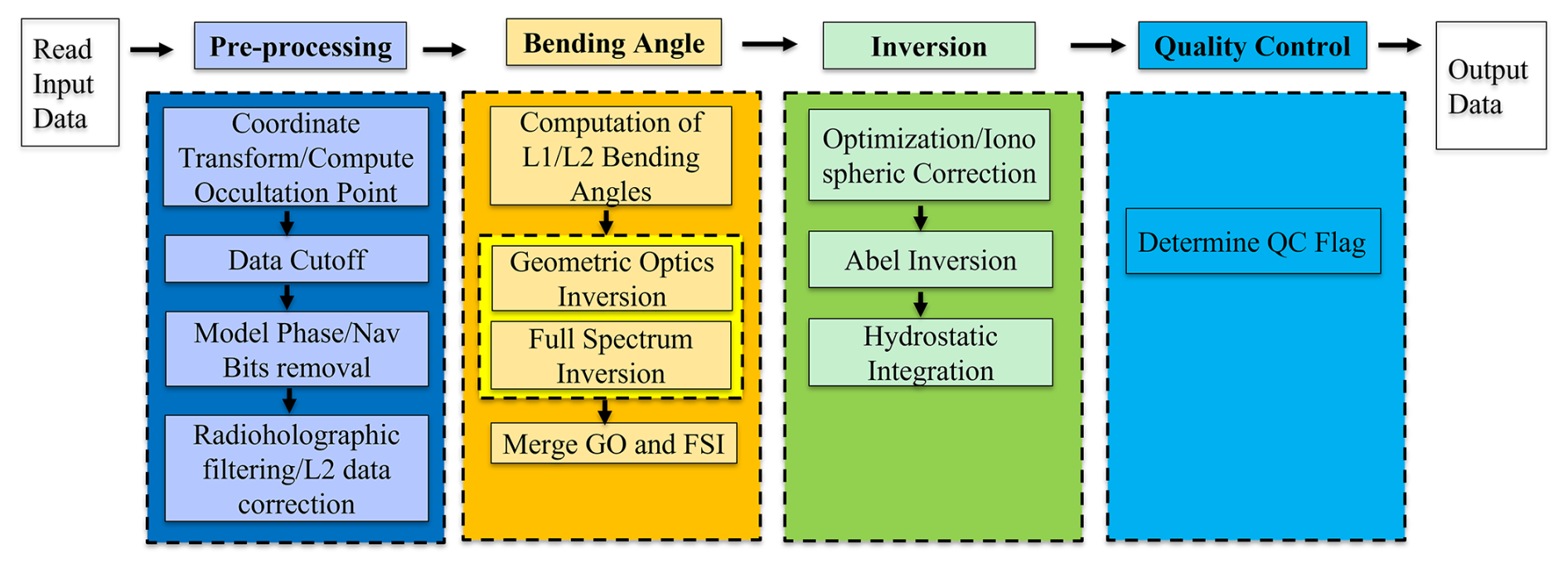
Figure 1 Flow chart depicting the steps used in the FSI RO data processing of the geometry and phase data.

The STAR RFSI end-to-end process involves four main steps (see Fig. 1):

1. data input and pre-processing: RO data, including satellite geometry, excess phase, and SNR measurements, are ingested and prepared for further processing. Satellite coordinates, if provided at lower frequencies, are interpolated to align with the sampling time using clock bias-corrected transmitter and receiver times (see Sect. 3.1).

2. bending angle calculation: excess phase data are converted to bending angles, with ionospheric corrections applied using dual-frequency measurements (see Sect. 3.2).

3. inversion to refractivity and dry temperature: bending angles are inverted using Abel integration to derive refractivity profiles, which can subsequently be used to compute dry atmospheric temperature (see Sect. 3.3).

4. quality control (QC): a comprehensive quality assessment is conducted by applying quality flags based on threshold criteria for bending angle differences, determined through comparisons with ERA5 simulations. This process ensures that only high-quality profiles are retained as valid (see Sect. 3.4). Additionally, we have developed an internal quality control system designed explicitly for near-real-time processing. This internal check was not included in the ROMEX data when it was generated.

Figure 1 illustrates the complete RO data processing workflow implemented in the STAR FSI system, highlighting the transition from raw signal acquisition to the generation of quality-controlled atmospheric profiles (bending angle and refractivity).

3.1 Data Input and Pre-processing

The STAR RFSI system ingests Level 1b dual-frequency excess phase and SNR data, along with satellite position and time information, to generate high-resolution atmospheric profiles. The geometry files typically contain satellite position vectors at a lower sampling rate (e.g., 1 Hz), whereas the excess phase and SNR are sampled at higher rates (e.g., 50–100 Hz). To align these data, satellite coordinates are interpolated to the excess-phase sampling times using clock-bias-corrected receiver and transmitter times. Satellite geometry and excess phase/SNR time series are interpolated into a common sampling rate. Given start time (t_s), sampling time (t), and clock bias-corrected receiver time (t_orb) and transmitter time (t_txm), the interpolated receiver coordinates (r_leo), transmitter time (t_txmHR), and GNSS coordinates (r_gns) can be calculated using cubic spline interpolation as:

$$\begin{array}{}\text{(1)}& {\displaystyle }& {\displaystyle }{r}_{\text{leo}}=\text{interpolate}(r_{\text{leoLR}},t_{\text{orb}},t+t_{\mathrm{s}},/\text{cubic\_spline})\text{(2)}& {\displaystyle }& {\displaystyle }{t}_{\text{txmHR}}=\text{interpolate}(t_{\text{txm}},t_{\text{orb}},t+t_{\mathrm{s}})\text{(3)}& {\displaystyle }& {\displaystyle }{r}_{\text{gns}}=\text{interpolate}(r_{\text{gnsLR}},t_{\text{txm}},t_{\text{txmHR}},/\text{cubic\_spline})\end{array}$$

where r_leoLR and r_gnsLR are the original coordinates.

The time series of satellite positions is initially provided in the Earth-Centered Inertial (ECI) J2000 frame. These positions are converted to Earth-Centered Earth-Fixed (ECEF) coordinates according to the IERS 2010 conventions, which include corrections for polar motion and Earth rotation (Adhikari et al., 2021; Petit and Luzum, 2010; Luzum and Petit, 2012). This transformation enables geolocation of the occultation tangent point at each time step.

To satisfy the assumption of local spherical symmetry during inversion, occultation geometry is reprojected to the local center of curvature. The tangent point location on the reference ellipsoid (WGS84) is determined where the straight line between the transmitter and receiver touches the ellipsoid. The latitude, longitude, local radius of curvature, and the center of curvature are computed at this reference tangent point and used to shift both GNSS and LEO positions into a local spherical coordinate system. This step ensures accurate mapping of impact parameters and tangent altitudes for each ray path.

RO signals acquired using OL tracking may contain low-SNR regions near the surface due to signal fading or tracking loss (see Fig. 5 in Adhikari et al., 2021). An appropriate cut-off height is essential to ensure the accuracy and reliability of tropospheric information retrieved from GNSS signals in OL tracking mode (Sokolovskiy et al., 2009, 2010; Adhikari et al., 2021; Paolella et al., 2025). To prevent the propagation of noise-contaminated signals through the inversion chain, a systematic signal truncation method is employed using SNR-based thresholds in this study. The truncation procedure includes the following steps: (1) initial cut-off impact height: the initial threshold of impact height is set based on the LEO satellite's altitude, as it influences the signal's penetration depth and the quality of retrieved atmospheric profiles; (2) dynamic background SNR calculation: the background SNR is estimated for each time series using the lowest 10 s of the smoothed data. A 3 s moving average is applied to the time series to smooth out high-frequency fluctuations; (3) initial SNR threshold determination: starting from the lowest point in the time series, the first point where the SNR exceeds three times the calculated background SNR in step (2) is identified as a preliminary threshold. (4) final cut-off point selection: moving backward from the uppermost point identified in step (3), the cut-off point is determined as the first point where the SNR drops below 1.5 times the background SNR, and the associated impact height is higher than the threshold established in step (1).

This filtering removes anomalous low-level SNR spikes, which can occur due to OL tracking artifacts, particularly in tropical and high-humidity conditions. Improper truncation can degrade the quality of bending angle measurements: truncating too high removes real signals, introducing a negative bias, while truncating too low retains noise, leading to oscillations in the retrieved profiles. The chosen thresholds aim to maximize vertical coverage without sacrificing data quality.

3.2 Computation of Bending Angles using Full Spectrum Inversion

Bending angle retrieval is performed in two steps: (1) computation of the model phase and correction of navigation bit jumps, and (2) inversion of observed signals using FSI to retrieve bending angles as a function of impact parameter.

3.2.1 Calculation of model phase

The model phase is derived from a reference refractivity profile computed using the MSIS-90 climatology (Hedin, 1991), assuming 90 % relative humidity below 15 km. Refractivity (N) is calculated as

$$\begin{array}{}\text{(4)}& N=\mathrm{77.6}{\displaystyle \frac{P}{T}}+\mathrm{3.73}\times {\mathrm{10}}^{\mathrm{5}}{\displaystyle \frac{e}{T^{\mathrm{2}}}}\end{array}$$

where P s pressure, T is temperature, and e is water vapor. The model impact parameter (a) at altitude z is calculated as

$$\begin{array}{}\text{(5)}& a=n(R+z)=nr\end{array}$$

where, $n=\mathrm{1}+N\times {\mathrm{10}}^{-\mathrm{6}}R$ is the local radius of curvature of the Earth, and $r=R+z$.

The bending angle (α) profile is derived from n and a using Abel integration

$$\begin{array}{}\text{(6)}& \mathit{\alpha }\left(p\right)=\mathrm{2}p\underset{r\mathrm{1}}{\overset{\mathrm{\infty }}{\int }}{\displaystyle \frac{a}{\sqrt{n^{\mathrm{2}}{r}^{\mathrm{2}}-a^{\mathrm{2}}}}}{\displaystyle \frac{\mathrm{d}\text{ln}\left(n\right)}{\mathrm{d}r}}\mathrm{d}r\end{array}$$

The impact parameter and bending angle profiles, along with occultation time (t), satellite positions, and velocities, are then used to derive the Doppler shift associated with the atmospheric refractivity n(z). The model phase, computed from occultation time and the Doppler shift, provides a reference for identifying navigation bit jumps.

In most RO data, navigation bits embedded in the excess phase and coordinate time series can introduce discontinuities of ± π. These phase jumps are identified by comparing the measured excess phase with the model phase, especially at high sampling rates (≥ 50 Hz). Once detected, the navigation bit pattern is applied to correct discontinuities in the measured phase, ensuring continuity and accuracy in the processed phase time series. Although the MSIS model is used to calculate the reference phase for these corrections, it introduces a known source of uncertainty in the lower troposphere. This uncertainty highlights the critical need for an external navigation bit stream, since standard navigation-bit-free cycle slip correction routines (such as those in ROPP) often struggle with atmospheric multipath in this region. To mitigate this issue, processing is often terminated above a 7–10 km impact height. However, this challenge can be circumvented by using pilot signals (Galileo E1C and E5BQ, GPS L2C, and BeiDou B1CP and B2AP), which are not modulated with navigation bits and can therefore yield reliable results in the lower troposphere even without external bit stream data (Jonathan Brandmeyer, personal communication, June 2025).

3.2.2 Full Spectrum Inversion

To retrieve bending angles from RO signals, it is essential to reduce high-frequency noise in the excess phase. This is typically achieved using low-pass or radio-holographic filters (Gorbunov et al., 2005). In the current RFSI inversion system, a 0.5 s low-pass Fourier filter is applied to the excess Doppler signal (the time derivative of excess phase). The filtered Doppler is then reintegrated to recover a smoothed excess phase. The 0.5 s window approximately matches the vertical resolution of RO observations, corresponding to the first Fresnel zone (Kursinski et al., 1997). To better resolve fine-scale refractivity structures in the lower atmosphere, a shorter, height-dependent smoothing window is used below 10 km: 0.05 s for 100 Hz data and 0.1 s for 50 Hz, enabling noise reduction while preserving small-scale features. The choice of these parameters is based on systematic tuning experiments in which multiple configurations were evaluated. The selected values showed here provide the most consistent statistical agreement with model outputs, such as ERA5, yielding reduced bending angle bias and standard deviation compared with other tested configurations.

Bending angles are computed using geometric optics (GO) above 25 km and the full spectrum inversion method below this altitude. In FSI, the received signal is expressed as a sum of narrowband sub-signals in the open-angle domain θ:

$$\begin{array}{}\text{(7)}& u\left(\mathit{\theta }\right)={\sum }_p{A}_p\left(\mathit{\theta }\right)e^{i{\mathit{\phi }}_{p\left(\mathit{\theta }\right)}}\end{array}$$

where, A_p and φ_p are the amplitude and phase of the pth sub-signal, respectively. The Fourier transform of Eq. (7) is:

$$\begin{array}{}\text{(8)}& F\left(\widehat{\mathit{\omega }}\right)={\sum }_p\underset{{\mathit{\theta }}_{\mathrm{1}}}{\overset{{\mathit{\theta }}_{\mathrm{2}}}{\int }}{A}_p\left({\mathit{\theta }}^{\prime }\right)e^{i({\mathit{\phi }}_p-{\widehat{\mathit{\omega }}}^{\prime })}\mathrm{d}{\mathit{\theta }}^{\prime }\end{array}$$

where θ₁ and θ₂ represent the open angles at the start and end of the occultation, respectively.

Applying the method of stationary phase (MSP) (Born and Wolf, 1999; Jensen et al., 2003), the transform simplifies to:

$$\begin{array}{}\text{(9)}& F\left(\widehat{\mathit{\omega }}\right)\approx B{e}^{i({\mathit{\phi }}_{\mathrm{q}}-{\widehat{\mathit{\omega }}}_{\mathrm{q}}{\mathit{\theta }}_{\mathrm{s}})}\end{array}$$

where B is an approximately constant amplitude, and the pseudo frequency ${\widehat{\mathit{\omega }}}_{\mathrm{q}}$ satisfies

$$\begin{array}{}\text{(10)}& {\widehat{\mathit{\omega }}}_{\mathrm{q}}={\displaystyle \frac{\mathrm{d}{\mathit{\phi }}_{\mathrm{q}}}{\mathrm{d}\mathit{\theta }}}{\mathrm{|}}_{\mathit{\theta }={\mathit{\theta }}_{\mathrm{s}}}\end{array}$$

The stationary points θ_s is then given by:

$$\begin{array}{}\text{(11)}& {\mathit{\theta }}_{\mathrm{s}}=-{\displaystyle \frac{\mathrm{d}\mathit{\psi }}{\mathrm{d}\widehat{\mathit{\omega }}}}\text{where }\mathit{\psi }={\mathit{\phi }}_{\mathrm{q}}-{\widehat{\mathit{\omega }}}_{\mathrm{q}}{\mathit{\theta }}_{\mathrm{s}}\end{array}$$

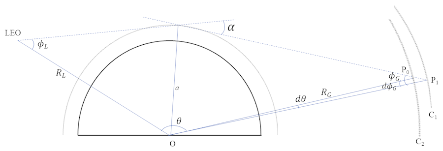
Figure 2 Projection of a non-circular orbit relative to the local center of curvature to a circular orbit.

The derivative of the phase (φ_q) with respect to θ, accounting for the signal path from the GNSS to LEO satellite, is:

$$\begin{array}{}\text{(12)}& \begin{array}{rl}{\displaystyle \frac{\mathrm{d}{\mathit{\phi }}_{\mathrm{q}}}{\mathrm{d}\mathit{\theta }}}={\widehat{\mathit{\omega }}}_{\mathrm{q}}=& ka+k{\displaystyle \frac{\mathrm{d}{R}_{\mathrm{L}}}{\mathrm{d}\mathit{\theta }}}\sqrt{\mathrm{1}-{\left({\displaystyle \frac{a}{R_{\mathrm{L}}}}\right)}^{\mathrm{2}}}\\ & +k{\displaystyle \frac{\mathrm{d}{R}_{\mathrm{G}}}{\mathrm{d}\mathit{\theta }}}\sqrt{\mathrm{1}-{\left({\displaystyle \frac{a}{R_{\mathrm{G}}}}\right)}^{\mathrm{2}}}\end{array}\end{array}$$

where k is the wavenumber of the carrier signal, R_L and R_G are the distances from the GNSS and LEO satellites to the local center of curvature, respectively, and a is the impact parameter.

Assuming circular orbits, the derivatives of R_L and R_G vanish, reducing Eq. (11) to:

$$\begin{array}{}\text{(13)}& {\displaystyle \frac{\mathrm{d}{\mathit{\phi }}_{\mathrm{q}}}{\mathrm{d}\mathit{\theta }}}=ka\end{array}$$

Differentiating with respect to $\widehat{\mathit{\omega }}$ gives:

$$\begin{array}{}\text{(14)}& \mathrm{d}a={\displaystyle \frac{\mathrm{1}}{k}}\mathrm{d}\widehat{\mathit{\omega }}\end{array}$$

The spectral resolution of the Fourier transform phase, $\mathrm{d}\widehat{\mathit{\omega }}$, is given by (Adhikari et al. 2016):

$$\begin{array}{}\text{(15)}& \mathrm{d}\widehat{\mathit{\omega }}={\displaystyle \frac{\mathrm{2}\mathit{\pi }}{\mathrm{\Delta }\mathit{\theta }}},\text{ where }\mathrm{\Delta }\mathit{\theta }={\mathit{\theta }}_{\mathrm{2}}-{\mathit{\theta }}_{\mathrm{1}}\end{array}$$

Finally, with the impact parameter a and the open angle θ, the bending angle is computed as:

$$\begin{array}{}\text{(16)}& \mathit{\alpha }\left(a\right)=\mathit{\theta }+\text{arcsin}\left({\displaystyle \frac{a}{R_{\mathrm{L}}}}\right)+\text{arcsin}\left({\displaystyle \frac{a}{R_{\mathrm{G}}}}\right)-\mathit{\pi }.\end{array}$$

3.2.3 Correction for non-spherical trajectory

The assumption underlying Eq. (14) is invalid in realistic occultation scenarios due to the Earth's oblateness and the non-coplanar nature of GNSS and LEO satellite orbits. To account for these effects, a correction must be applied to the observed phase to project the signal path onto circular, coplanar trajectories. As illustrated in Fig. 2, the actual GNSS satellite orbit is represented by arc C₁, with each point along the trajectory projected onto a circular orbit, C₂. Notably, the impact parameter (a) remains unchanged during this projection. In this process, the GNSS position is shifted from P₁ on arc C₁ to P₀ on arc C₂. This projection alters the open angle (θ), the signal ray (ϕ_G), and the phase of the signal. Although Fig. 2 focuses on the GNSS orbit, the same projection method is also applied to the LEO receiver orbit. Given the known positions of the GNSS and LEO satellites, the resulting changes in phase and open angles can be determined geometrically. Note that the radius and center of curvature are treated as fixed for a given RO event and are not dynamically reprojected. The projection is performed with respect to the precomputed local center of curvature, ensuring a consistent coordinate system throughout the inversion process.

After calculating bending angles for the L1 and L2 frequencies separately, the profiles are truncated using the FSI amplitude. This step is necessary because the FSI method produces bending angle and impact parameter pairs over an infinite range of impact parameters. Determining the lowest impact parameter and its corresponding bending angle is critical. In the current STAR FSI inversion approach, the pair with the lowest impact parameter and bending angle is identified based on the amplitude of the Fourier transform. The amplitude is first normalized using the signal's mean amplitude within the 10–50 km range. The lowest point is defined as the altitude at which the normalized amplitude drops below 0.35. This threshold is empirically determined based on extensive testing within the STAR FSI system. It represents an optimal balance between maximizing vertical penetration depth and minimizing noise-induced artifacts into the retrieved bending angle profile.

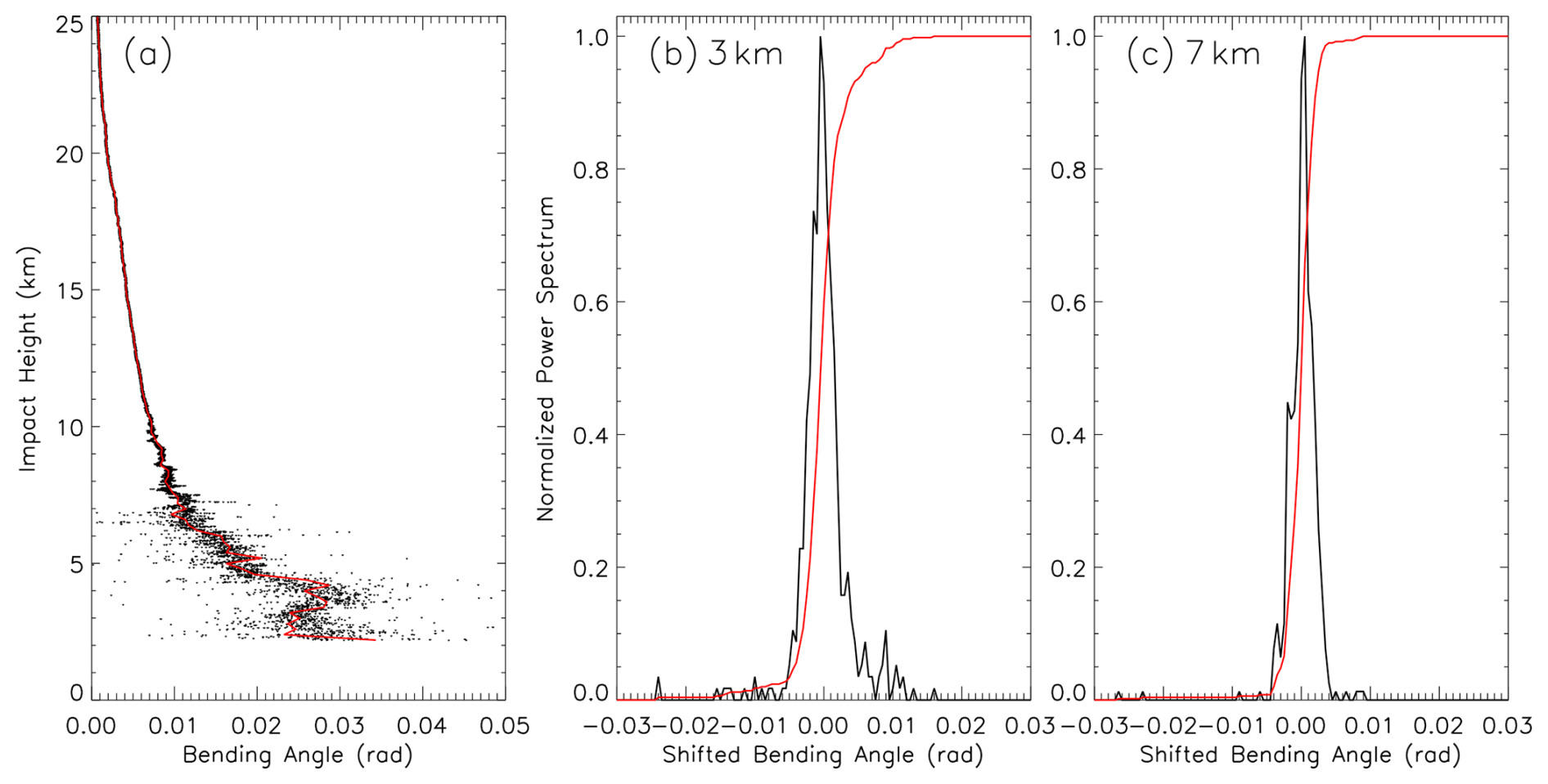
Figure 3 (a) Spectrogram of the RO signal, power spectrum at (b) 3 km, and (c) 7.5 km impact heights.

3.2.4 Bending Angle Uncertainty Calculation

The uncertainty in the bending angle is estimated using a sliding spectrogram with a 500 m window. First, a smoothed bending angle profile is generated to identify the central component. Then, the bending angle from the unsmoothed signal is calculated at 1 m impact height resolution. With each spectral window, deviations from the central component are used to construct a local power spectrum of the shifted bending angle, computed using a finite bending angle increment (δα = 0.0005 rad). The shifted bending angle (α_s), is defined as the instantaneous bending angle minus the central component. The spectral width (Δs) is determined as the mean of the absolute value of the shifted bending angle weighted by the spectral power (ρ) of each component, as follows (which is similar to Liu et al., 2018):

$$\begin{array}{}\text{(17)}& \mathrm{\Delta }s=\sqrt{{\displaystyle \frac{{\sum }_{i=\mathrm{1}}^n{\mathit{\rho }}_{\mathrm{i}}{\mathit{\alpha }}_{\mathrm{s}}^{\mathrm{2}}\mathit{\delta }\mathit{\alpha }}{{\sum }_{i=\mathrm{1}}^n{\mathit{\rho }}_{\mathrm{i}}\mathit{\delta }\mathit{\alpha }}}}\end{array}$$

Figure 3a presents a representative bending angle profile at 1 m resolution as a function of the impact height (black dots), along with its central component (red line). Figure 3b and c show the corresponding normalized power spectrum (black line) and accumulated power spectrum (red line) at impact heights of 3 and 7 km, respectively. As illustrated, the spectral range at 3 km is broader than at 7 km, indicating greater atmospheric variability at lower altitudes. The bending angle uncertainty is quantified as half the spectral width, calculated using Eq. (15).

3.3 Bending angle Inversion

3.3.1 Ionospheric Correction and Optimization

To remove first-order ionospheric effects, and as an approximation for the neutral atmosphere bending angle, a linear combination of L1 and L2 bending angles (α₁(a) and α₂(a)) is computed (Vorob'ev and Krasil'nikova, 1994):

$$\begin{array}{}\text{(18)}& {\mathit{\alpha }}_{\text{LC}}\left(a\right)={\displaystyle \frac{{\mathit{\alpha }}_{\mathrm{1}}\left(a\right)f_{\mathrm{1}}^{\mathrm{2}}-{\mathit{\alpha }}_{\mathrm{2}}\left(a\right)f_{\mathrm{2}}^{\mathrm{2}}}{f_{\mathrm{1}}^{\mathrm{2}}-f_{\mathrm{2}}^{\mathrm{2}}}}\end{array}$$

where f₁ and f₂ are the RO frequencies.

This is followed by statistical optimization (Gorbunov, 2002c):

$$\begin{array}{}\text{(19)}& \mathit{\alpha }\left(a\right)={\mathit{\alpha }}_{\text{BG}\left(a\right)}+{\displaystyle \frac{{\mathit{\sigma }}^{\mathrm{S}}}{{\mathit{\sigma }}^{\mathrm{S}}+{\mathit{\sigma }}^{\mathrm{N}}}}\left({\mathit{\alpha }}_{\text{LC}}\right(a)-{\mathit{\alpha }}_{\text{BG}}(a)\end{array}$$

where, σ^S and σ^N are the covariances of the neutral atmospheric signal and residual noise, respectively, and α_BG(a) is the background bending angle from a climatological model (MSIS-90 model).

Covariance matrices are estimated from the deviation (Δα) of L1 and L2 bending angles from the background model (${\mathit{\alpha }}_{L\mathrm{1},L\mathrm{2}}-{\mathit{\alpha }}_{\mathrm{m}}$). For ionospheric signal and noise, deviations in the impact heights (impact parameter minus local center of curvature) of 50–70 km are used; for neutral atmospheric signal, the 12–35 km range is used. In the lower troposphere, near the surface, where the L2 signals weaken, a constant correction is applied based on the lowest valid L2 altitude.

3.3.2 Abel Inversion

Refractivity is retrieved from ionosphere-corrected bending angles using the Abel transform (Fjeldbo et al., 1971). The bending angle profile is extended up to 150 km using climatological data (MSIS-90 model) to stabilize the upper boundary condition. Tangent point locations are recovered by interpolating the occultation time and satellite positions. Since time information is lost during the Fourier transform of the RO signal, the occultation time is reconstructed from the bending angle-impact parameter profile and used to infer the latitude and longitude of each tangent point.

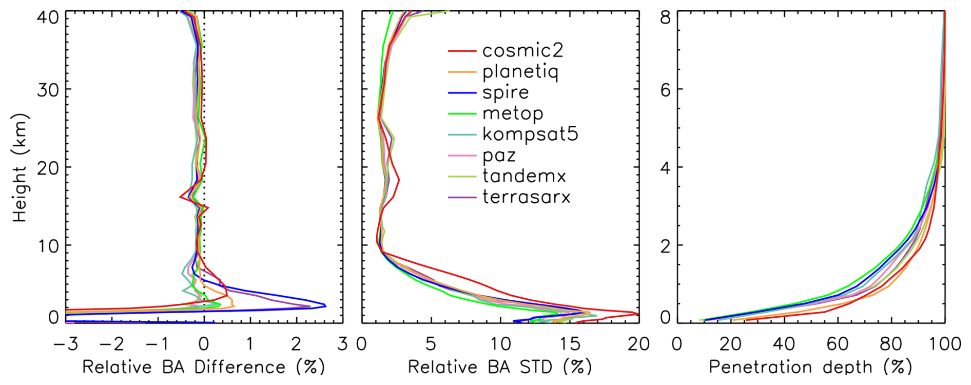
Figure 4 Comparison of height-dependent fractional bending angle between RO observations and ERA5 simulations (O−B) among different RO missions. BA mean biases (left), standard deviations (middle) in terms of fractional BA difference (%), and (right) penetration depth below 8 km for RFSI over November 2022.

3.4 Quality control

Due to the lack of effective internal quality control in the ROPP v10 package, we rely on external quality control procedures to identify bad profiles. The fractional difference between the observed (O) and simulated (B) bending angles, calculated from ERA5 forecast fields, is used to assess the quality of the RO data at each altitude level:

$$\begin{array}{}\text{(20)}& {\text{BA}}_{\text{diff}}={\displaystyle \frac{O-B}{B}}\end{array}$$

The annual mean standard deviation (σ_year) from 2020 is used as a benchmark. A profile is flagged as “bad” if the bending angle difference exceeds 7σ_year at any altitude level between 10 and 40 km, where RO data quality is highest and model-observation agreement is strongest. A sensitivity study confirmed that using a 7σ year threshold provides an optimal balance between data retention and data quality.

In addition, profiles are also flagged as “bad” under any of the following conditions: (1) The fractional BA difference exceeds 7σ_year; (2) The top height of the profile is below 20 km; (3) The bottom height is above 20 km; and (4) A negative bending angle is detected below 50 km. The QC rejection rate for the ROMEX dataset depends on the mission. For example, the QC pass rates are 85.7 %, 94.8 %, and 93.9 % for COSMIC-2, Spire, and PlanetiQ, respectively. These values are comparable to those from CDAAC-processed data: 87.6 %, 95.7 %, and 90.6 %, respectively. Note that quality control is not applied to PlanetiQ and Spire data processed by EUMETSAT. To ensure a consistent comparison in this study (Sect. 4), we applied our standard quality control procedure to the EUMETSAT dataset where quality control was absent.

It is important to note that this quality control procedure applies only to bending angles within a specific height range (10–40 km). In rare cases, even when the bending angle passes QC, anomalies in refractivity or dry temperature may still occur due to limitations in the Abel inversion. Future updates to the QC procedures will address such issues. This process ensures that only high-quality profiles are retained as valid. An internal quality control system tailored for near-real-time processing is under development; however, it was not incorporated into the ROMEX data when that dataset was produced.

4 Comparison Results

4.1 Bending angle comparison with STAR RFSI, STAR ROPP, and EUMETSAT

Figure 4 shows the height-dependent fractional bending angle differences between RO observations and ERA5 background fields (O−B) for multiple satellite missions processed using the RFSI algorithm during November 2022. The selected missions include COSMIC-2, Spire, PlanetiQ, Metop-B, Metop-C, Kompsat5, PAZ, TerraSAR-X, and TanDEM-X. The comparison serves as a proxy for evaluating the quality and inter-mission consistency of RFSI-processed RO data relative to a widely used global reanalysis.

In the middle and upper troposphere through the lower stratosphere (8–35 km), all missions exhibit excellent agreement with ERA5. Mean O−B differences are generally within ± 0.2 %, and standard deviations remain below 3 %, indicating high internal consistency among the RO datasets and strong alignment with ERA5 in this well-observed atmospheric region.

In the lower troposphere (below 8 km), larger biases and variability are evident, especially near the surface. Spire and TerraSAR-X show mean biases up to 1 %–2 % at 2 km, with standard deviations exceeding 10 %. COMSIC-2 exhibits the highest variability in this region, with standard deviations approaching 20 % at approximately 1 km. These discrepancies are likely attributed to increased atmospheric variability in the lower troposphere, limitations in signal tracking during multipath propagation at tropical/subtropical regions where high water vapor variability makes OL tracking difficult, and the sensitivity of bending angle retrievals to SNR cut-off thresholds. In contrast, PlanetiQ, Metop-B, and Metop-C demonstrate smaller near-surface biases (typically < 0.5 %) and reduced variability, suggesting robust signal tracking and/or more effective pre-processing of low-altitude data.

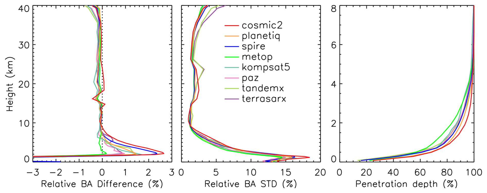
Figure 5 Same as Fig. 4, but for RO data generated from the ROPP package using the CT2 method.

Above 35 km, mean biases increase to approximately 0.6 %, and standard deviations increase with height and can exceed 5 % at 40 km. These deviations are primarily due to limitations in ionospheric correction at higher altitudes, where residual ionospheric effects are more challenging to remove completely. The ionospheric conditions during September-November 2022 were generally moderate and typical for the ascending phase of Solar Cycle 25, but intermittently disturbed (including several geomagnetic storms and enhanced irregularities). They are not representative of worst-case conditions, but also not purely quiet-average; they are better described as moderately active with episodic disturbances.

Among the evaluated missions, PlanetiQ consistently shows low mean biases and standard deviations across nearly the entire vertical range, indicating strong data stability and processing robustness. Metop-B and Metop-C also exhibit excellent performance, likely due to mature sensor platforms and the use of well-established pre-processing procedures in the ROPP system. Spire data, while reliable in the mid- to upper troposphere, shows elevated near-surface variability, likely due to its higher sensitivity to excess phase pre-processing (e.g., cycle-slip removal and parameter tuning).

COSMIC-2 displays distinct behavior relative to other missions, with positive biases of 8–35 km and increased variability near the tropopause. These features are likely influenced by its low-inclination orbit and limited latitudinal coverage (± 45°), which concentrates observations in tropical and subtropical regions with higher atmospheric variability. Similar features and their impact on data assimilation performance have been discussed in previous studies (Ho et al., 2023; Miller et al., 2025).

The penetration depth is defined as the minimum height above ground level where a valid (i.e., not filled or missing) bending angle or refractivity is obtained for a given RO event. Smaller penetration depths indicate that the RO signal reaches closer to the Earth's surface. Penetration depth depends on the signal cutoff criteria applied during processing (see Sects. 3.1 and 3.2.3); therefore, comparisons among different missions should be made using the same processing center and algorithm. The right panel of Fig. 4 shows the penetration depth profile below 8 km, expressed as the percentage of profiles reaching different altitudes relative to 8 km, for the FSI method. As discussed by Gorbunov et al. (2022a, b), higher SNR generally improves tropospheric penetration. Consistent with Table 2, COSMIC-2 and PlanetiQ exhibit the greatest penetration depth among the missions. Most missions achieve more than 80 % of occultations reaching 2 km or lower, and more than 50 % reaching 1 km or lower. The penetration depths are noticeably higher for Metop-B and Metop-C (green line), while Spire, despite having the lowest SNR, achieves a slight better penetration than Metop.

Figure 5 shows O−B bending angle differences for the same missions and period, but with data processed using the STAR ROPP-CT2 method. The vertical structure of mean biases and variability is broadly similar to that in the RFSI results, reflecting consistent retrieval behavior between the two approaches. In the 8–35 km range, both methods yield small biases (within ± 0.2 %) and standard deviations below 3 %, confirming the reliability of both retrievals in the core atmospheric region. One exception is KOMPSAT-5, which shows a slight negative bias (∼ −0.2 %) between 17 and 23 km.

Standard deviations increase above 35 km and below 8 km in both datasets, highlighting common challenges in the upper and lower atmospheric regions, including multipath effects, signal noise, and uncertainty in ionospheric corrections. However, the CT2 retrievals generally exhibit larger near-surface biases than those of RFSI. For all missions except Metop-B and Metop-C, the CT2-processed profiles exhibit biases of 1 %–2 % near the surface, likely due to the more conservative use of signals and stronger smoothing.

In contrast to Fig. 4, the penetration depth profiles among missions are much narrower below 1 km, indicating that CT2 is less sensitive to SNR. Consistent with Fig. 4, COSMIC-2 and PlanetiQ show the deepest penetration depth among the missions. The penetration depths are noticeably higher for Metop-B and Metop-C than for Spire.

Figure 6 Same as Fig. 4, but for RO data provided from EUMETSAT.

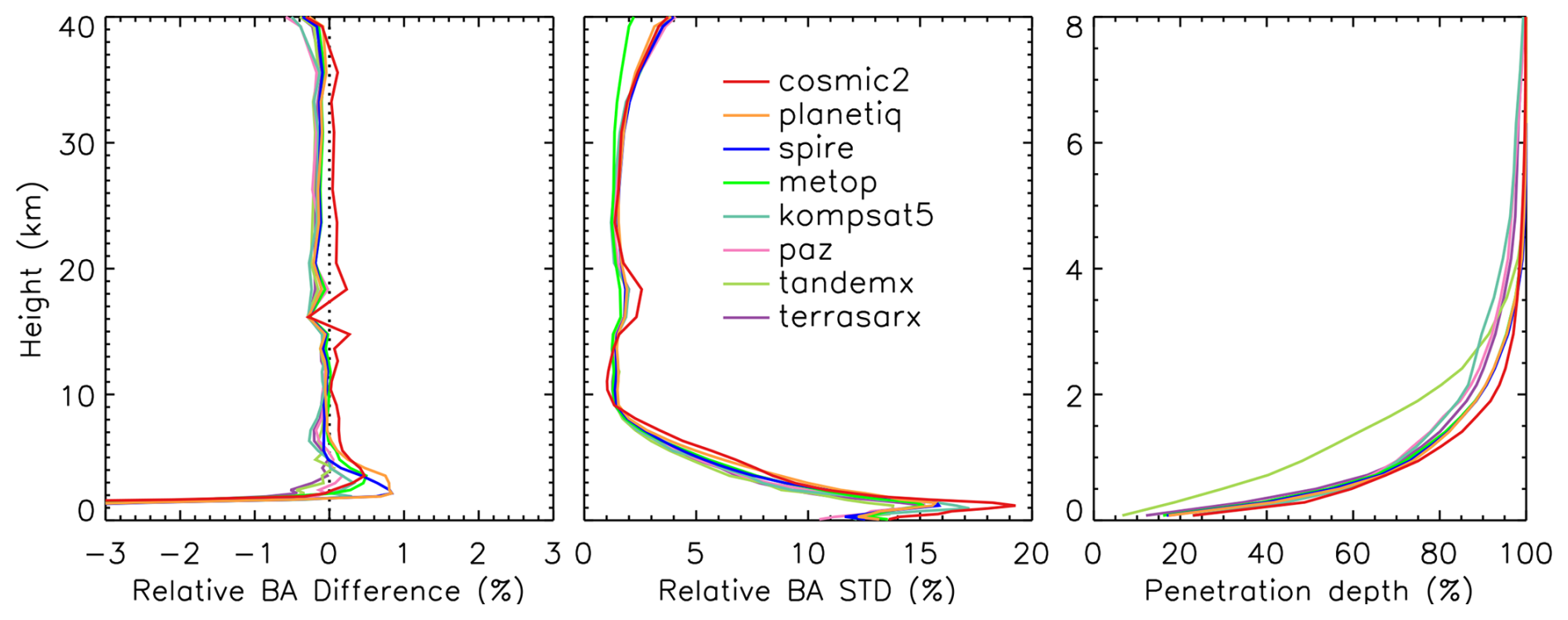
Figure 6 displays ERA5 O−B differences for RO profiles processed by EUMETSAT, covering the same missions and period. The EUMETSAT-processed data (excluding COSMIC-2) utilized ROM SAF ROPP as the internal processing system, employing the CT2 method in the troposphere. Consistent with the other two datasets, EUMETSAT results show high consistency in the 8–35 km range, with mean biases within ± 0.2 % and standard deviations below 3 %. COSMIC-2 again stands out, showing a positive bias of ∼ 0.2 %, while most other missions exhibit slightly negative biases, suggesting a systematic offset in COSMIC-2 data relative to the ensemble.

In the lower troposphere, EUMETSAT retrievals exhibit the smallest mean biases (< 1 % at 2 km) among the three datasets, suggesting more effective mitigation of noise and multipath effects near the surface. By comparison, RFSI-processed profiles for Spire and TerraSAR-X show near-surface biases of up to ∼ 2 %, while STAR ROPP CT2 retrievals yield 1 %–2 % biases for most missions. COSMIC-2 exhibits high variability below 8 km across all three datasets, although the CT2 method appears to reduce it slightly. Note that while STAR ROPP and EUMETSAT ROPP both use CT2 method in the troposphere, their specific configuration parameters may differ.

Above 35 km, the bending angle uncertainty increases in all datasets. However, EUMETSAT results exhibit more uniform performance across missions, with mean biases generally below 0.5 % and smaller inter-mission variability. Metop-B and Metop-C show the lowest standard deviations across all datasets in this altitude range, indicating highly stable performance at high altitudes.

The penetration depth from TanDEM-X is noticeably higher than that of other missions in the EUMETSAT-processed data. For Metop-B and Metop-C, penetration depths are substantially improved compared with STAR FSI and STAR ROPP CT2, and approach those of COSMIC-2 and PlanetiQ below 1.5 km.

The comparatively shallower penetration depths observed for Metop (in Fig. 5) and TanDEM-X (in Fig. 6) relative to missions like COSMIC-2 and PlanetiQ are linked to a combination of mission-specific characteristics (specifically SNR) and the data truncation strategies employed by the processing algorithm: (1) Impact of lower SNR: Penetration depth is fundamentally dependent on the signal cutoff criteria applied during processing, and higher SNR is known to improve tropospheric penetration. Metop-B/C and TanDEM-X exhibit lower mean SNRs (e.g., Metop-B GPS SNR is 730.2, TanDEM-X is 549.3) compared to the missions with the deepest penetration (COSMIC-2 at 1295.1 and PlanetiQ at 1440.5). This lower SNR makes them more susceptible to noise and multipath effects in the lower troposphere, leading to a shallower signal cutoff. (2) Truncation strategy: The systematic signal truncation used in the STAR RFSI method is based on SNR thresholds to prevent noise-contaminated signals from propagating. For lower-SNR missions like Metop and TanDEM-X, these thresholds are reached at higher altitudes, resulting in shallower penetration. (3) Processing algorithm variation: The choice of processing algorithm also contributes to variation. The CT2 method, used in both ROPP systems (STAR ROPP and ROM SAF ROPP), is less sensitive to SNR and resulted in generally narrower penetration depth profiles below 1 km compared to RFSI. This is further reflected by the fact that Metop-B/C penetration is substantially improved when processed by EUMETSAT's CT2 compared to STAR's algorithms, suggesting differences in the specific configuration parameters used by the processing centers.

Together, these intercomparisons highlight key trade-offs among the different retrieval approaches. The RFSI method leverages the full frequency content of the RO signal, offering enhanced sensitivity to fine-scale atmospheric features. However, it is also more sensitive to noise, particularly near the surface. In contrast, the STAR ROPP CT2 method employs a canonical transformation that simplifies retrieval but is more conservative in its use of signal data, resulting in smoother profiles and slightly larger near-surface biases. EUMETSAT's processing strikes a balance between these extremes, achieving consistent results across the full vertical range while effectively suppressing noise in the lower troposphere and upper stratosphere.

4.2 Refractivity comparison with STAR RFSI, STAR ROPP, and EUMETSAT

Figure 7 presents the fractional refractivity differences between RO observations processed using the RFSI algorithm and ERA5 background fields for November 2022. The vertical structures of refractivity O−B statistics largely mirror those of the bending angle differences shown in Fig. 4, reflecting the propagation of bending angle quality into the refractivity retrieval. In the well-constrained 8–30 km region, all missions show excellent agreement with ERA5. Mean biases remain within ± 0.15 %, and standard deviations are typically below 1 %, indicating that refractivity retrievals in this core region retain the stability and consistency of the underlying bending angle data.

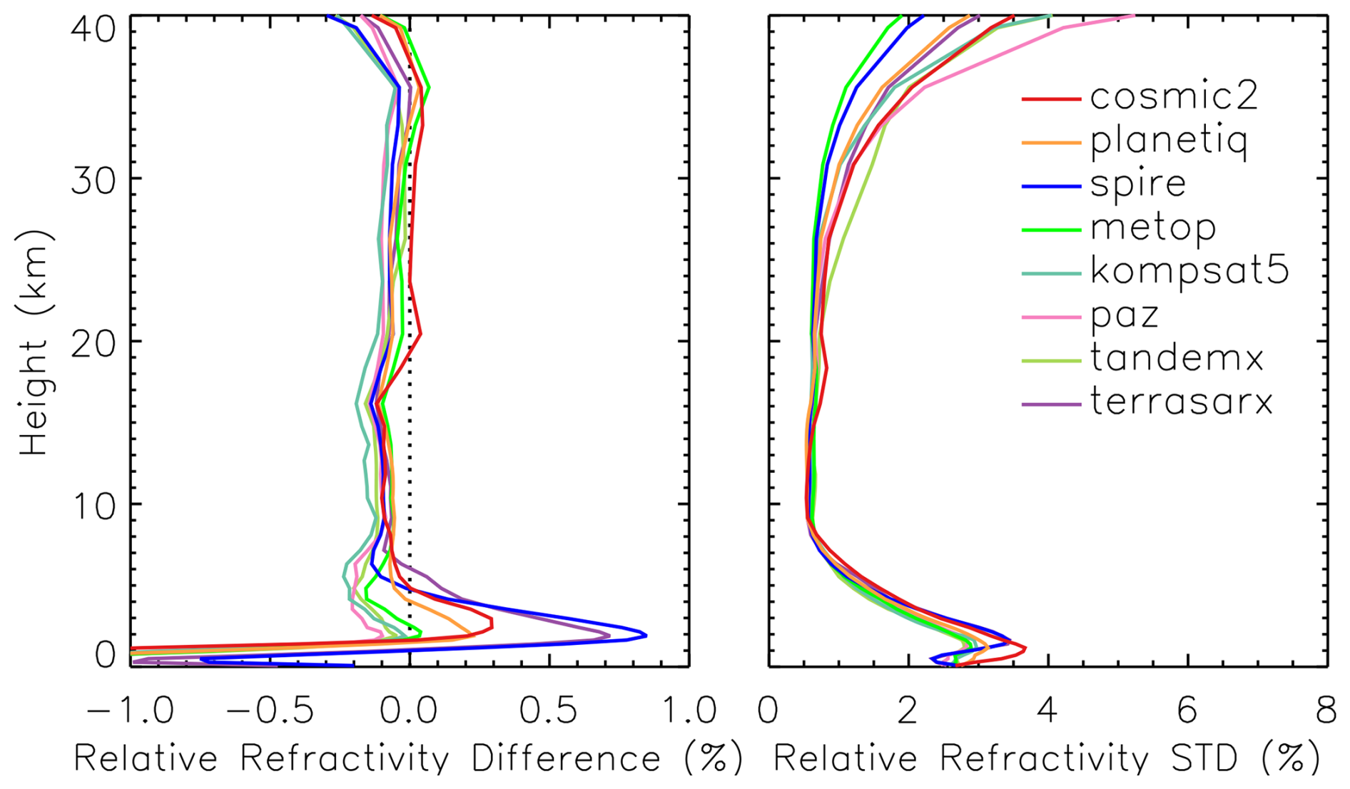
Figure 7 Comparison of height-dependent fractional refractivity between RO observations and ERA5 simulations (O−B) among different RO missions. Refractivity mean biases (left) and standard deviations (right) in terms of fractional difference (%) for RFSI over November 2022.

In the lower troposphere (below ∼ 8 km), refractivity differences exhibit a significantly larger inter-mission spread, consistent with Fig. 4, although both biases and standard deviations are generally reduced. Spire and TerraSAR-X exhibit the most pronounced positive biases, reaching ∼ 0.7 %–0.8 % near 2 km, along with elevated standard deviations exceeding 3 %. COSMIC-2 again exhibits high variability below 5 km, with standard deviations peaking at over 3.5 % near 1 km. However, its mean refractivity bias remains relatively small compared to those from Spire or TerraSAR-X, suggesting increased random error rather than systematic offset.

In the upper atmosphere (above ∼ 35 km), where refractivity is less sensitive to the RO signal due to the exponential decrease in atmospheric density, the mean biases for all missions begin to increase negatively, reaching values of ∼ −0.2 % to −0.4 % near 40 km. Standard deviations also rise, ranging from ∼ 2 % to 5 %, consistent with the increased variability observed in the bending angle differences shown in Fig. 4. These errors are primarily attributed to residual ionospheric correction uncertainties and the influence of high-altitude extrapolation assumptions in the RFSI algorithm. The use of climatological models in the upper atmosphere also introduces additional variability, as refractivity becomes more sensitive to model inaccuracies in this region.

Figure 8 shows the refractivity O−B differences derived from RO data processed with the ROPP CT2 method. Between 8 and 15 km, CT2 results exhibit improved inter-mission consistency in mean bias compared to RFSI, although the standard deviations are generally larger. In the lower troposphere (below ∼ 8 km), CT2 retrievals produce larger positive biases, typically around 0.5 %–1 % near 2 km (except for Metop-B, Metop-C, and TerraSAR-X), with the largest bias observed for COSMIC-2 (∼ 1 %). These biases are notably larger than those from RFSI, which remain below 0.3 % for most missions, except for Spire and TerraSAR-X. Between 15–25 km, the CT2 results show a greater inter-mission spread in both mean bias and standard deviation compared to RFSI. Above 25 km, CT2 and RFSI show broadly similar behavior, with rising uncertainty consistent with bending angle trends. Note that both RFSI and CT2 used geometric optics method above 25 km.

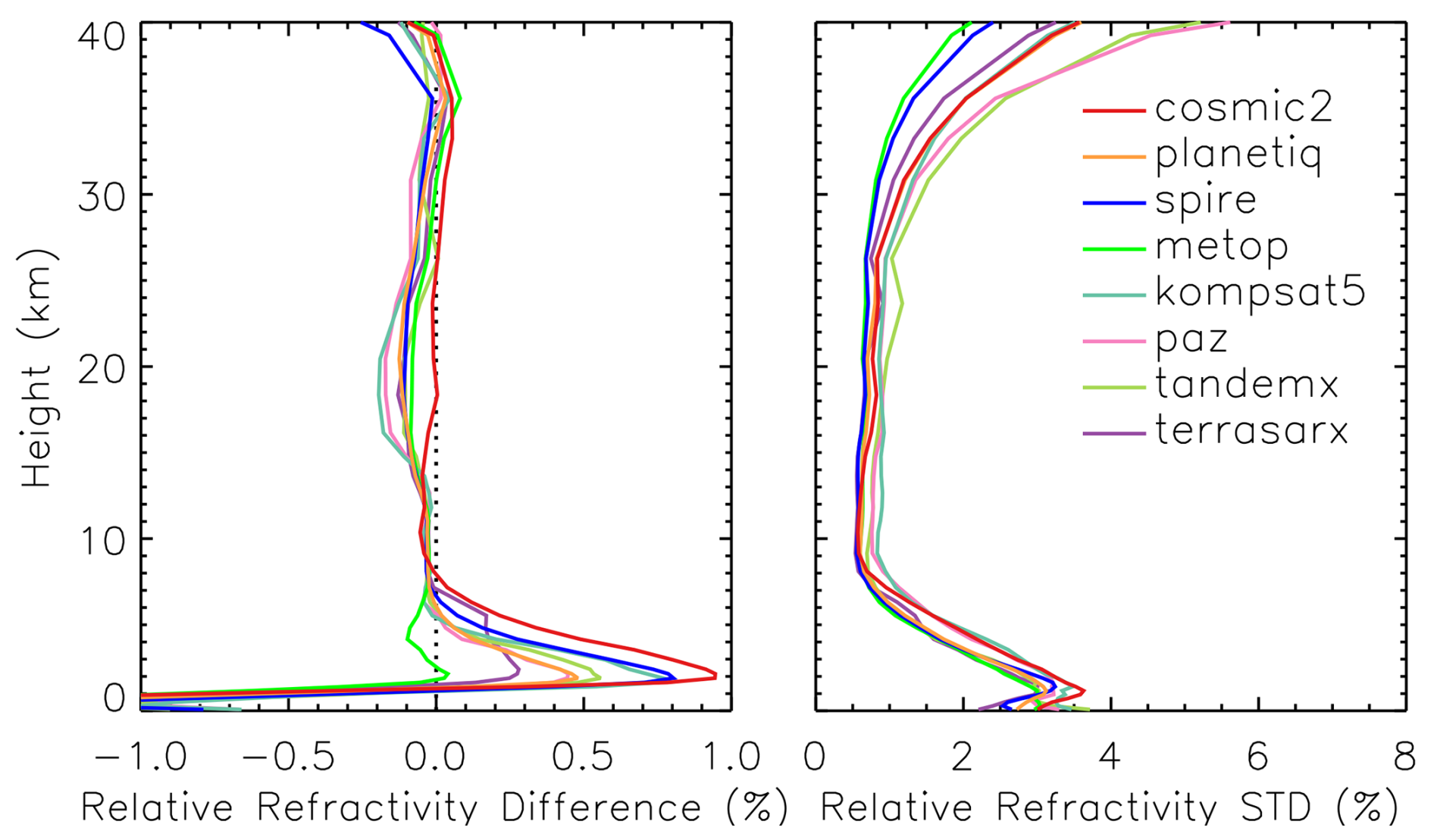
Figure 8 Same as Fig. 7, but for RO refractivity processed using the ROPP package with the CT2 method.

Figure 9 presents the refractivity O−B differences from the EUMETSAT dataset. Note that refractivity profiles are not available for PlanetiQ and Spire in this dataset. Similar to bending angle results, COSMIC-2 exhibits a distinct positive bias in the 4–30 km region, along with a notably larger inter-missions spread in the 8–40 km range compared to CT2 (Fig. 8) and RFSI (Fig. 7) results. In contrast, in the lower troposphere (below ∼ 8 km), the EUMETSAT retrievals show the smallest near-surface mean biases, generally within ± 0.2 % above 2.5 km, and the lowest standard deviation across all available missions. These results suggest that the refractivity data from EUMETSAT are particularly effective at mitigating noise and multipath effects near the surface.

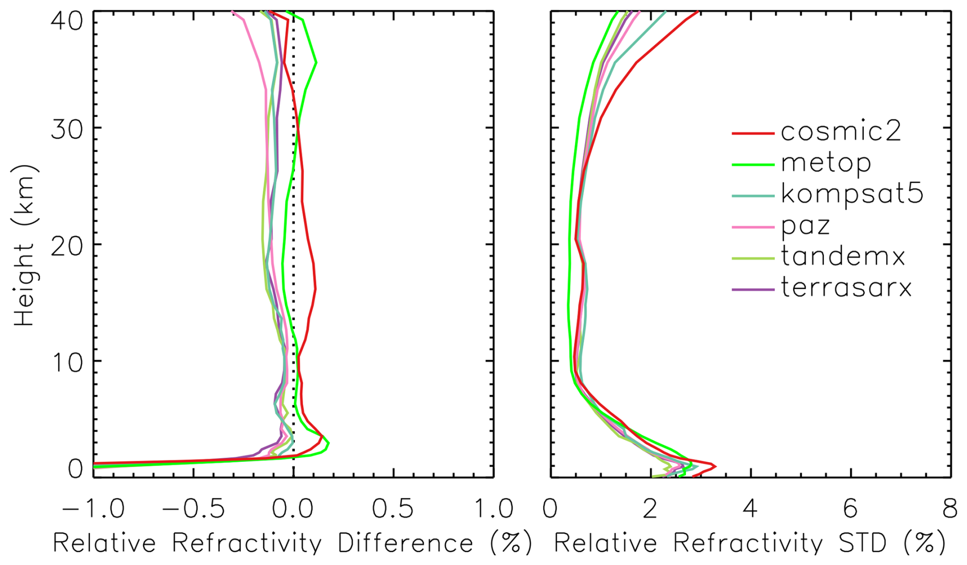
Figure 9 Same as Fig. 7, but for RO data provided from EUMETSAT. Note that refractivity data is not available in the EUMETSAT dataset for PlanetiQ and Spire.

Taken together, the comparisons between Figs. 4 and 7, Figs. 5 and 8, and Figs. 6 and 9 reveal that many mission-specific features observed in bending angle retrievals persist in the refractivity domain. This reinforces the importance of bending angle quality, particularly near the surface and in the upper atmosphere, for achieving accurate refractivity retrievals. The heightened sensitivity of refractivity to small-scale errors at the profile boundaries also underscores the need for robust quality control, optimized signal tracking, and careful algorithm design in future RO missions and processing systems.

4.3 Structural Uncertainty among Different Processing Methods

Figure 10–14 illustrate the structural bending angle uncertainty associated with the ROPP (CT2), RFSI, and EUMETSAT processing algorithms for five representative GNSS RO missions: COSMIC-2, Spire, PlanetiQ, Metop-B, and Metop-C. For each mission, the figure shows the height-dependent relative mean differences and standard deviations of bending angles with respect to the three-dataset mean, along with the number of common profiles processed for each algorithm.

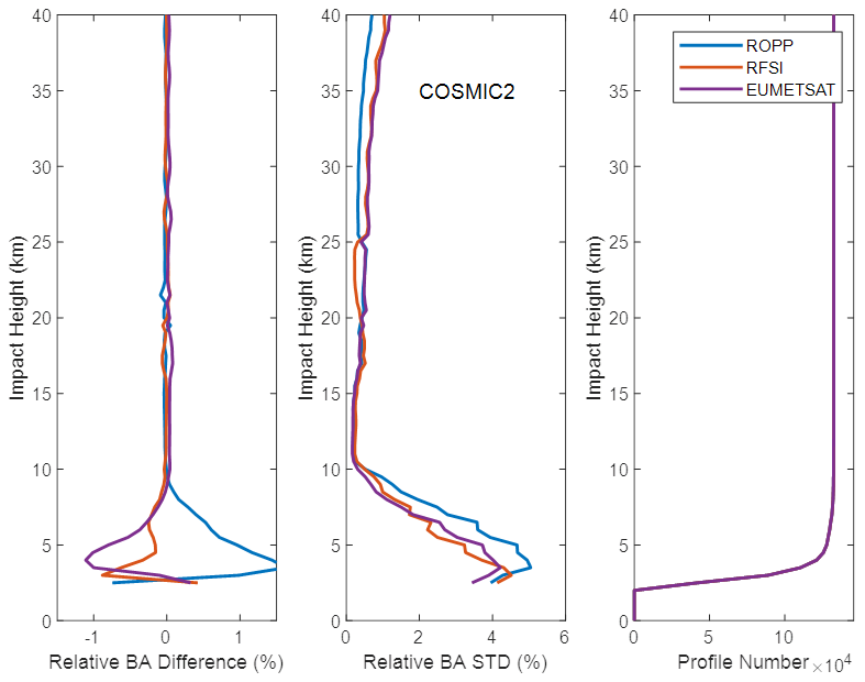
Figure 10 Structural bending angle uncertainty among different processing methods for COSMIC-2. Note that the bending angle profiles from the EUMETSAT dataset are processed by the UCAR CDAAC using the phase-matching method.

Several important structural differences emerge from these comparisons:

For COSMIC-2 (Fig. 10), the three processing methods demonstrate strong consistency in the middle and upper troposphere and stratosphere (above ∼ 10 km), where both the relative differences and standard deviations of bending angles remain below approximately 0.1 % and 1 %, respectively, indicating minimal structural uncertainty. Below 10 km, method-dependent differences become more pronounced. The largest deviations are observed near the surface, with relative differences of approximately 1.5 % for ROPP, −1.0 % for EUMETSAT, and −0.5 % for RFSI. Additionally, the ROPP algorithm exhibits higher bending angle standard deviations in the lowest 10 km, indicating greater sensitivity to retrieval ambiguities under conditions of multipath propagation. In contrast, above 25 km, ROPP shows slightly lower standard deviations than RFSI and EUMETSAT. Despite these lower-tropospheric differences, the overall structural agreement among the three COSMIC-2 processing methods is robust. Although the number of available profiles (right panel) decreases significantly near the surface, sufficient observations are present throughout the vertical domain to enable meaningful statistical comparisons.

Figure 11 Same as Fig. 10, but for Spire.

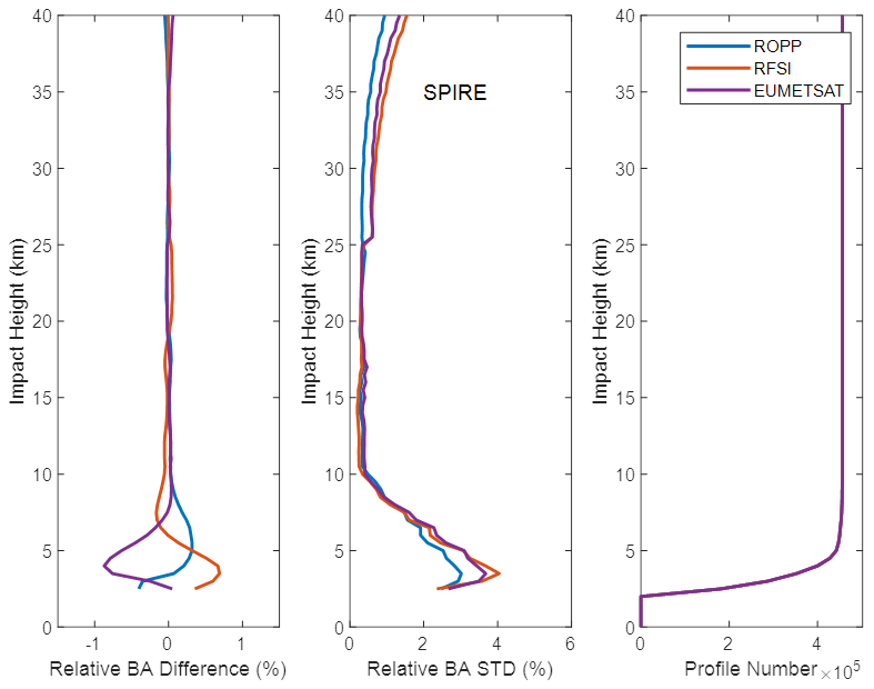
For Spire (Fig. 11), a similar pattern of agreement is observed. Above approximately 10 km, the relative bending angle differences across the three methods are generally within ± 0.1 %, and the standard deviations remain below 1 % up to approximately 35 km, indicating good consistency in the upper atmosphere. However, RFSI exhibits a distinct pattern in the 8–25 km range, with a relative positive difference in the 19–25 km region and a negative difference in the 8–19 km region, compared to the nearly identical ROPP and EUMETSAT solutions. As with COSMIC-2, larger discrepancies emerge below 10 km. Notably, the ROPP and RFSI solutions show small positive differences near the surface (up to ∼ 0.7 % and ∼ 0.3 %, respectively), whereas the EUMETSAT solution exhibits a negative deviation of up to −1.0 %. The bending angle standard deviations in the lower troposphere are higher for RFSI and EUMETSAT, reaching ∼ 4 %, while ROPP shows slightly lower variability (below 3 %) near the surface. Above 25 km, ROPP again yields lower standard deviations compared to the other two methods, consistent with the COSMIC-2 results.

Figure 12 Same as Fig. 10, but for PlanetiQ.

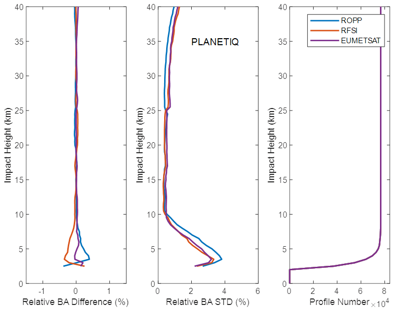
For PlanetiQ (Fig. 12), a higher level of consistency is observed among the three processing methods across the vertical profile compared to those from COSMIC-2 and Spire. Above ∼ 10 km, the solutions are nearly identical, except for a slight positive deviation in the 19–25 km region from the RFSI solution. Relative bending angle differences remain within ± 0.05 %, and standard deviations are below 1 % up to ∼ 38 km, indicating excellent agreement in the middle and upper atmosphere. Below 10 km, small but systematic differences become evident. The ROPP solution shows a modest positive bias, peaking at approximately +0.4 % near a 3 km impact height, while the RFSI solution exhibits a slight negative bias of similar magnitude. The EUMETSAT data remain close to zero throughout this region. As with COSMIC-2, the standard deviations increase toward the surface, with ROPP exhibiting greater variability below 10 km than RFSI and EUMETSAT. However, for PlanetiQ, the overall variability is lower, reaching a standard deviation of ∼ 3 % near the surface. This improved consistency suggests enhanced robustness in PlanetiQ's onboard processing, a more stable tracking geometry and antenna design, and higher SNR, which may reduce sensitivity to differences among retrieval algorithms.

Figure 13 Same as Fig. 10, but for Metop-B.

Figure 14 Same as Fig. 10, but for Metop-C.

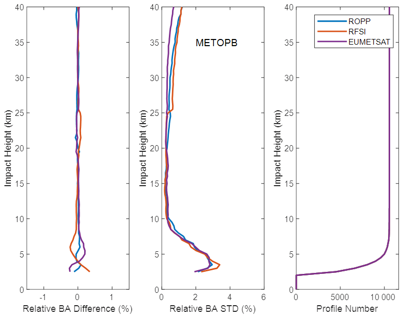
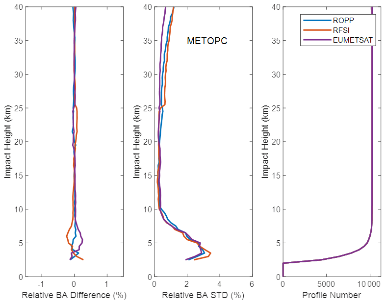
Metop-B (Fig. 13) and Metop-C (Fig. 14), both long-operational polar-orbiting satellites with mature and well-characterized instrumentation, exhibit nearly identical inter-method structural uncertainties. For brevity, the discussion here focuses on Metop-B. Below an impact height of ∼ 8 km, the standard deviation profiles from all three algorithms converge closely, indicating similar variability near the surface. Relative bending angle differences show a maximum positive deviation of approximately +0.2 % for the EUMETSAT solution and a negative deviation of about −0.2 % for RFSI near 5 km.

In contrast, the ROPP solution remains close to zero. A slight negative bias is also observed in the RFSI solution below ∼ 13 km (∼ −0.1 %). In the upper stratosphere, above 25 km, a clear separation in variability emerges: RFSI exhibits the largest standard deviations, followed by ROPP, with EUMETSAT showing the lowest variability. This divergence in STD differences near 25 km for Metop-B/C, compared to COSMIC-2, PlanetiQ, and Spire, suggests that the upper-atmospheric retrievals for Metop-B/C are more sensitive to processing methodology. This is supported by the data showing that in the upper stratosphere (above 25 km), the EUMETSAT algorithm exhibits the lowest variability. Given that Metop-B/C are EUMETSAT missions and their data are routinely processed by EUMETSAT, this superior performance suggests that the EUMETSAT processing methodology is likely fine-tuned and highly stable for their mature sensor platforms, enabling effective mitigation of noise and uncertainties at high altitudes, and resulting in the lowest variability observed across all datasets.

Except for COSMIC-2, RFSI shows a small positive bias (< 0.1 %) at 20–25 km for Spire, PlanetiQ, and Metop-B/C relative to STAR ROPP and EUMETSAT. Possible causes include spectral windowing and filtering choices, as RFSI applies a sliding polynomial filter below 25 km and an optimal estimation filter above 25 km, potentially introducing systematic offsets. Degraded L2 signals and reduced GNSS SNR at ∼ 20–25 km further amplify noise, and because FSI is more noise-sensitive than geometric optics or canonical transform methods, incomplete noise suppression may yield small positive biases. The exact causes are under active investigation to further mitigate this effect.

These results highlight that structural uncertainty is both algorithm- and mission-dependent, influenced by signal quality, onboard processing, antenna design, and orbit characteristics. The findings highlight the crucial role of processing methodology in ensuring consistency and accuracy in retrieving RO bending angle data, particularly when data from diverse missions are used in operational weather forecasting systems. Future efforts in GNSS RO should focus on developing harmonized processing standards and conducting inter-comparison studies to quantify and mitigate structural uncertainty in bending angle datasets.

5 Discussions and Summary

This study presents the first comprehensive cross-mission intercomparison of the STAR-developed Full Spectrum Inversion algorithm with the community-standard ROPP CT2 and EUMETSAT dataset within the framework of ROMEX. Using bending angle and refractivity profiles from key GNSS RO missions (e.g., COSMIC-2, Spire, PlanetiQ, Metop-B/C) during the ROMEX period (September–November 2022), we assessed inter-algorithm consistency against ERA5 reanalysis and structural uncertainty against the three-dataset mean.

A significant finding is the excellent agreement among all three processing methods in the middle and upper troposphere and lower stratosphere (8–35 km). In this region, the mean bending angle differences remained within ± 0.2 % and the standard deviations were below 3 %, demonstrating the maturity and robust internal coherence of RO observations across diverse missions. Similarly, refractivity retrievals in this core region exhibited high stability, with mean biases within ± 0.15 % and standard deviations typically below 1 %.

Anthes et al. (2025) reported that the UCAR-processed COSMIC-2 bending angles included in ROMEX exhibit a positive bias of approximately 0.1 %–0.15 % relative to ERA5 in the lower stratosphere, larger than the biases seen for Spire and other ROMEX datasets. Similar lower-stratospheric positive biases for UCAR COSMIC-2 have also been documented by Ho et al. (2024, 2025). This difference is predominantly a representativeness effect associated with orbit-dependent sampling over a non-spherical Earth (the azimuth effect), rather than a true systematic bias, and therefore does not significantly impact data assimilation. The remaining small component (less than 0.05 %) is attributed to the sideways displacement of the occultation plane and can be mitigated by impact height correction during RO processing (Anthes et al., 2025). Figure 15 provides a zoomed-in comparison of the height-dependent fractional O−B bending-angle differences for the COSMIC-2, Spire, and PlanetiQ missions, between the EUMETSAT/UCAR processing and the STAR RFSI processing. In Fig. 15a, the COSMIC-2 data are from UCAR, while the Spire and PlanetiQ datasets are processed by EUMETSAT; in Fig. 15b, all three missions are processed consistently by STAR RFSI.

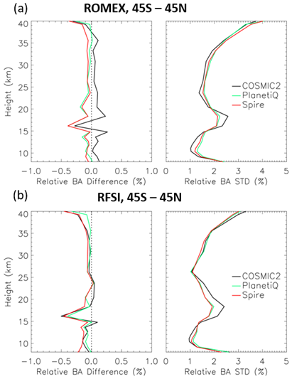
Figure 15 Zoomed-in height-dependent fractional bending-angle differences (O−B) between RO observations and ERA5 simulations are shown for COSMIC-2, Spire, and PlanetiQ. Panels (a) and (b) display the mean bending-angle biases (left) and standard deviations (right) for RO data processed by EUMETSAT and by STAR RFSI, respectively.

While the UCAR-provided COSMIC-2 ROMEX datasets show a small positive O−B bias compared to EUMETSAT-processed Spire and PlanetiQ data in the lower stratosphere (Fig. 15a), the STAR RFSI-processed COSMIC-2 bending angles exhibit improved consistency with the Spire and PlanetiQ results (Fig. 15b). One contributing factor may be the treatment of horizontal tangent-point sliding within the RFSI framework. While a consistent occultation point definition is applied across missions in this study, differences in occultation point definitions (or georeferencing) among processing centers can affect the magnitude of the sliding-related correction. As noted in Anthes et al. (2025), UCAR defines the occultation point as the location where the L1 excess phase exceeds 500 m, typically in the lower troposphere. In contrast, RFSI defines it as the location where the straight-line tangent altitude equals zero, typically in the upper troposphere-lower stratosphere (UTLS). This sideways sliding effect can introduce a positive bias in COSMIC-2 bending angles of up to ∼ 0.05 %. The underlying cause of the subtle differences in the lower-stratospheric O−B bending-angle among the processing centers (STAR, EUMETSAT, UCAR) will be examined further in future work.

Conversely, larger discrepancies and heightened variability emerged in the lower troposphere (below ∼ 8 km) and upper atmosphere (above ∼ 35 km). These regions are challenged by multipath effects, increased tracking noise, and varying SNR. The FSI method, designed to resolve fine-scale atmospheric structures by leveraging full-spectrum signal information, demonstrated improved sensitivity in the lower atmosphere (Adhikari et al., 2021), particularly for missions such as PlanetiQ and Metop-B/C. However, it also showed increased variability and greater dependence on SNR cut-off and quality control thresholds, as seen with Spire and TerraSAR-X near the surface. In contrast, the CT2 method, while generally yielding smoother profiles with reduced noise, sometimes showed larger near-surface biases (e.g., CT2 for COSMIC-2 and Spire), suggesting a more conservative approach that might underestimate bending in complex conditions. EUMETSAT's dataset, in particular, achieved the smallest near-surface bending angle and refractivity biases across missions, indicating effective mitigation of noise and multipath.

A crucial finding of this study is that structural uncertainty depends on both the processing algorithm and the satellite mission. A greater inter-method spread was observed across all missions below 8 km, likely due to their distinct approaches to handling multipath, noise, and signal truncation. This structural uncertainty complicates the consistent use of multi-mission RO data. For instance, COSMIC-2 data processed by ROPP CT2 showed higher near-surface variability than those processed by RFSI and EUMETSAT. In contrast, missions like Metop-B/C exhibited stronger consistency across all three methods, while PlanetiQ demonstrated the highest inter-method consistency throughout the profile. These mission-specific patterns, clearly illustrated in Figs. 10–14, underscore the critical need to characterize and account for algorithmic effects when assimilating multi-mission RO data into operational weather forecasting systems. The explicit comparison of the total O−B standard deviation (Figs. 4–6) with the structural uncertainty (Figs. 10–14) quantifies the contribution of retrieval algorithm differences to the total error budget, demonstrating that structural differences account for approximately one-fourth of the total O−B standard deviation over all the altitudes, providing a critical metric for interpreting ROMEX forecast impact studies and refining GNSS RO data assimilation systems.

The ROMEX results unequivocally highlight the importance of quantifying algorithm-related structural uncertainty for data assimilation applications. To ensure a consistent and optimal representation of RO data in numerical weather prediction systems, it may be necessary to harmonize retrieval strategies across different processing centers or to apply mission- and algorithm-specific bias corrections.

The successful integration of STAR's FSI algorithm into ROPP version 10.0 represents a significant advancement, providing users with a robust and flexible alternative to existing algorithms. This enhancement facilitates consistent RO data processing across both government-funded and commercial missions, offering customizable settings to meet specific scientific and operational requirements.

In summary, this study demonstrates the critical influence of algorithm choice, particularly in the lower troposphere; confirms strong consistency among processors in the mid-to-upper atmosphere; identifies distinct mission-dependent structural uncertainties; and recommends applying bias correction or ensemble strategies to improve data assimilation. The findings strongly support continued efforts to harmonize across agencies through collaborative initiatives, such as ROMEX. As the volume and diversity of GNSS RO data continue to expand, these insights underscore the paramount need for robust algorithm development, thorough uncertainty quantification, and coordinated processing strategies to fully leverage RO observations and advance weather forecasting and climate monitoring capabilities.