A new approach to inversion of multi-spectral data with applications to FUV remote sensing

Many atmospheric measurement techniques involve inversion of photon counts detected by multi-spectral sensors spanning the X-ray to microwave regions of the electromagnetic spectrum. Although photon counts follow Poisson statistics, commonly used inversion techniques often rely on statistical assumptions that disregard the Poisson nature of the sensor data, limiting the scientific utility of datasets. Motivated to overcome this limiting assumption, this study focuses on retrieval techniques that involve the ratio of counts received in different sub-bands and introduces a new computationally efficient and robust approach to this type of inverse problem that respects the underlying count statistics. The method assumes that the received photon counts in each channel are a realization of a binned point process, allowing the ratio of the channel intensities to be modeled within a hierarchical Bayesian framework. This allows us to directly incorporate correlation between the bins via the prior that is modeled using a permanental process. It further enables more accurate uncertainty quantification without costly sampling procedures common in Bayesian inversion methods. The method is verified and validated on thermospheric column-integrated neutral temperature retrievals from simulated top-of-atmosphere far-ultraviolet (FUV) disk emission data corresponding to 2–8 November 2018, which includes a minor geomagnetic storm. The sub-bands associated with the N₂ Lyman-Birge-Hopfield (2,0) transition are used for the ratio calculation. The method is also demonstrated on calibrated photon counts data from the NASA Global-scale Observations of the Limb and Disk (GOLD) mission from the same time period and from 11 May 2024 during a severe geomagnetic storm. The study demonstrates the method's ability to accurately recover neutral temperature in a variety of geophysical conditions, attesting to its potential to extend the fidelity of neutral temperature retrievals over a broader range of solar zenith angles (0–100°), compared to the current limit of (0–80°) available with existing techniques.

1 Introduction

In recent decades, far-ultraviolet (FUV) remote sensing has played a key role in advancing space physics by providing valuable measurements of space plasma and neutral species. In the upper atmosphere, these emissions are primarily caused by various physical processes such as photoionization, photoexcitation, charge exchange and recombination that depend on thermospheric composition and temperature and ionospheric plasma density. The fact that these FUV emissions are observable from space without contending with significant background emissions makes FUV remote sensing attractive for upper atmosphere research (Paxton et al., 2017). In particular, the Lyman-Birge-Hopfield (LBH) bands, which arise from the transition ${\mathrm{N}}_{\mathrm{2}}(a^{\mathrm{1}}{\mathrm{\Pi }}_g,v^{\prime })\to {\mathrm{N}}_{\mathrm{2}}(X^{\mathrm{1}}{\mathrm{\Sigma }}_g^{+},v^{\prime \prime })$, where $(v^{\prime },v^{\prime \prime })$ denote the vibrational levels of the upper (excited electronic) and lower (ground electronic) states, are some of the most prominent emission features in the FUV spectrum. Short-wavelength N₂ LBH bands, such as (3,0) and (2,0), are absorbed by O₂, so their observed emissions decrease with increasing O₂ density. Comparing these absorbed bands to less-absorbed bands allows retrieval of the O $/$ N₂ composition ratio in the thermosphere. The rotational structure of N₂ LBH bands, arising from transitions between rotational levels within the upper a¹Π_g and lower $X^{\mathrm{1}}{\mathrm{\Sigma }}_g^{+}$ electronic states, can be used to retrieve the thermospheric temperature. Temperature and compositions are fundamental physical properties of the upper atmosphere and are important parameters for space weather research due to their relationship to aerodynamic drag experienced by objects in low Earth orbit (e.g., Aksnes et al., 2006; Doornbos and Klinkrad, 2006; Krywonos et al., 2012; Leonard et al., 2012; Emmert, 2015; Zesta and Huang, 2016; Mehta et al., 2023). Current inverse modeling techniques, however, often make assumptions on the statistical nature of photon count data that are especially problematic when photon counts are low, such as when solar zenith angle (SZA) is large. Even when photon counts are moderate to high, inversion techniques assuming Gaussian statistics have been observed to introduce bias into retrievals that can be on the order of statistical uncertainty (e.g., Humphrey et al., 2009; Yamada et al., 2019; Nicolaou et al., 2024). Additionally, commonly used inversion techniques do not take into account the spatial structure of the photon count sensor data, limiting their ability to recover the underlying spatially correlated physical parameters.

One class of inversion methods used to estimate properties of the thermosphere from FUV emissions is based on ratios of total observed counts in sub-bands of the received spectra. For example, changes in the shape of the LBH bands are correlated with the changes in ambient temperature (e.g., Aksnes et al., 2006), and the ratios of some of these channels have been shown to have an approximately linear relationship with temperature under typical geophysical conditions (e.g., Cantrall and Matsuo, 2021). Ratio-based techniques are widely used for $\mathrm{\Sigma }\mathrm{O}/{\mathrm{N}}_{\mathrm{2}}$ and QEUV data products using the ratio of atomic oxygen and LBH emissions (e.g., Strickland et al., 1995; Zhang et al., 2004; Meier, 2021; Correira et al., 2021) as well as estimates of ionospheric structure (Yin et al., 2023). Outside of FUV sensing, these techniques are also used in LiDAR profiling (Jia and Yi, 2014), spectrometry (Coath et al., 2013), x-ray astronomy (Park et al., 2006; Jin et al., 2006; Wang et al., 2024), astrochemistry (Boersma et al., 2012), and synthetic aperture radar (Gallardo i Peres et al., 2024), among others. The relative simplicity of the two-channel ratio inversion techniques makes them amenable to integration of spatial models.

Following the work by Jin et al. (2006) and Park et al. (2006), we reformulate the problem of estimating a quantity of interest from ratios of disjoint channels as a hierarchical Bayesian inference problem. Specifically, the photon count data are used to infer the ratio of Poisson means, which we consider the geophysically relevant variable. This formulation allows us to rigorously characterize the effect of shot noise on the estimate of channel means, leading to a better understanding of the uncertainties in the estimates due to the shot noise. It is particularly relevant to upper atmosphere FUV remote sensing as shot noise effects are a major source of uncertainty in the radiance measurements from which the GOLD mission data products are retrieved, including the neutral temperature (McClintock et al., 2020; Evans et al., 2024b). Additionally, this new formulation facilitates explicitly introducing spatial structure into the estimation by treating the received photon count data as a realization of a Poisson point process (Streit, 2010).

Among a variety of methods proposed to estimate the Poisson intensity from point process data, including the work by Nowak and Kolaczyk (2000); Antoniadis and Bigot (2006); De Oliveira (2013), we choose to model the intensity with a permanental process model (McCullagh and Møller, 2006), allowing us to use the theory of reproducing kernel Hilbert spaces to recover the intensity and perform uncertainty quantification (Flaxman et al., 2017; Walder and Bishop, 2017). Once the ratio of Poisson means Z is estimated, the effective neutral temperature is then recovered using the approximate linear relationship (Cantrall and Matsuo, 2021)

$$\begin{array}{}\text{(1)}& Z\approx m{T}_{\mathrm{eff}}+z_{\mathrm{0}}\end{array}$$

where T_eff is the effective neutral temperature and m and z₀ are slope and intercept parameters that depend on the specific LBH band and the observation geometry. These parameters are fit using the Budzien vibrational-rotational model (Budzien et al., 2001). The method is verified and validated with simulated GOLD disk emission photon count data generated using an instrument simulator (Cantrall, 2022) and the NOAA Whole Atmosphere Model (WAM, Akmaev, 2011) for 2–8 November 2018. The method is furthermore demonstrated on calibrated, geolocated photon count data collected by GOLD for the same time period, as well as data from the Gannon storm in May 2024 (Grandin et al., 2024). These examples show that the proposed new approach is able to accurately retrieve the column-integrated temperature in a wide variety of geophysical conditions, both during geomagnetically quiet and severely disrupted periods, and attest to the potential for extending temperature retrievals with uncertanty quantification based on the LBH band emission to higher SZAs than currently made available. In addition, the method yields robust results with a computational cost that is feasible as an operational algorithm. Specifically, it achieves a full characterization of the posterior distribution of the neutral temperature without computationally intense sampling procedures that are common in Bayesian inversion methods. The method is implemented in an R package (R Core Team, 2025) that is publicly available (LeDuc and Matsuo, 2026).

In Sect. 2 we introduce the statistical modeling framework for temperature inference. In Sects. 3 and 4, we illustrate the new inversion procedures on simulated and actual GOLD disk emission data, respectively. Section 5 contains discussion of the computational performance, as well as directions for future research. Lastly, in Sect. 6 we provide the conclusion.

2 Hierarchical Bayesian Inverse Method

In this section, we derive the inversion procedure as a hierarchical Bayesian method and discuss potential sources of error in the procedure. Since this work is motivated by estimation of thermospheric column-integrated neutral temperature from channel ratio data, we focus on that particular application. However, we believe that this method is more generally applicable due to the other areas where channel ratio data are used in inverse problems described previously.

2.1 Building on Previous Work: The Forward Model

We seek to estimate the column-integrated thermospheric temperature from the top-of-atmosphere LBH band emission sensed by the GOLD instrument. Specifically, photon counts from radiometrically calibrated, geolocated L1C GOLD science data products are considered (McClintock et al., 2020). The column-integrated (effective) temperature T_eff can be given as a function of the wavelength λ as

$$\begin{array}{}\text{(2)}& T_{\mathrm{eff}}\left(\mathit{\lambda }\right)={\displaystyle \frac{{\int }_{\mathrm{0}}^{\mathrm{\infty }}V(r,\mathit{\lambda })\exp (-\mathit{\tau }(r,\mathit{\lambda }\left)\right)T_n\left(r\right)\text{d}r}{{\int }_{\mathrm{0}}^{\mathrm{\infty }}V(r,\mathit{\lambda })\exp (-\mathit{\tau }(r,\mathit{\lambda }\left)\right)\text{d}r}}\end{array}$$

where r (cm) is the slant path distance, $V(\mathrm{photons}\times {\mathrm{s}}^{-\mathrm{1}}{\mathrm{cm}}^{-\mathrm{3}}$) is the LBH volume emission rate, τ the optical depth, and T_eff (K) the neutral temperature (Evans et al., 2024b). This represents a weighted average of the neutral temperature along the line of sight, with the weight determined by the product $V(r,\mathit{\lambda })\exp (-\mathit{\tau }(r,\mathit{\lambda }\left)\right)$. The LBH volume emission rate depends on neutral temperature, collisional quenching by O₂ and other species, and the local excitation rate from electron impact or solar radiation (Solomon, 2017; Cantrall and Matsuo, 2021). Since LBH emissions derive from the same electronic transition of N₂ and there is only a weak wavelength dependence in absorption, effective temperature is nearly independent of wavelength in the LBH system. As shown in Fig. 4 of Evans et al. (2024b), the most weight is assigned to altitudes around 120–200 km. Since these observations are integrated quantities, they cannot be assigned to a specific altitude without a-priori knowledge of the temperature structure (e.g., Cantrall et al., 2019; Cantrall and Matsuo, 2021; Evans et al., 2024b). Despite this limitation, the NASA GOLD mission data product of column-integrated temperature (TDISK) has broad scientific applications and has been widely used in research (Evans et al., 2024b).

The forward modeling of the neutral temperature is based on the vibrational-rotational band model (Budzien et al., 2001), which supplies laboratory LBH spectra across a range of neutral temperatures given vibrational populations of N₂. For the purposes of the study, we use the populations in Ajello et al. (2020), which are derived from laboratory data. The modeled spectra are convolved with the spectral point-spread function of the instrument to approximate the intensities as seen by the detector. Principal component analysis of simulated GOLD data has shown that under typical geophysical conditions the intensity in the upper portion of the LBH (2,0) band, from wavelength 138.56–139.2 nm, is positively correlated with temperature, while the intensity in the lower portion from 138–138.56 nm is negatively correlated with temperature (Cantrall and Matsuo, 2021). A similar structure is shown to hold in the (1,1) and (2,3) bands as well (Cantrall et al., 2019). So, as the column-integrated temperature increases, the observed photon counts in the upper portion of the band increases while the observed counts in the lower portion of the band decrease. This leads to the approximately linear relationship between the ratio of the long wavelength to short wavelength portions of the band and the neutral temperature (Cantrall and Matsuo, 2021), which is used in the study. As noted in Zhang et al. (2019) and Cantrall and Matsuo (2021), two-channel ratio approaches have several potential advantages. These include the ease of calculating a ratio compared to fitting a full spectral model and the traceability of uncertainty by not requiring knowledge of variation in instrument performance across the whole band, rather just a small section of it (Cantrall and Matsuo, 2021).

2.2 Modeling the Intensity Ratio

The first step is to model the two-channel intensity ratio as a random process. To motivate the choice of model we first consider the case where the inversion is done without consideration to spatial or temporal correlation, as in Park et al. (2006) and Jin et al. (2006). Throughout the remainder of the paper, the notation X∼F means that the random variable X has the distribution F. If we assume that the count data from the channels are independently Poisson distributed with different mean parameters Λ_a and Λ_b, so that

$$\begin{array}{}\text{(3)}& \begin{array}{rl}\mathit{\left\{}{a}_i{\mathit{\}}}_{i=\mathrm{1}}^{n_a}\right|{\mathrm{\Lambda }}_a& \sim \mathrm{Poisson}\left({\mathrm{\Lambda }}_a\right)\\ \mathit{\left\{}{b}_i{\mathit{\}}}_{i=\mathrm{1}}^{n_b}\right|{\mathrm{\Lambda }}_b& \sim \mathrm{Poisson}\left({\mathrm{\Lambda }}_b\right)\end{array}\end{array}$$

then the posterior distribution of the ratio $Z={\mathrm{\Lambda }}_a/{\mathrm{\Lambda }}_b$ given the data is a generalized Beta-Prime distribution $BP(\mathit{\alpha },\mathit{\beta },p,q)$, which has a density of the form

$$\begin{array}{}\text{(4)}& p_Z\left(z\right)={\displaystyle \frac{p}{qB(\mathit{\alpha },\mathit{\beta })}}{\displaystyle \frac{(z/q{)}^{\mathit{\alpha }p-\mathrm{1}}}{(\mathrm{1}+(z/q{)}^p{)}^{\mathit{\alpha }+\mathit{\beta }}}}\end{array}$$

if z>0, and 0 elsewhere, where $\mathit{\alpha }>\mathrm{0},\mathit{\beta }>\mathrm{0},p>\mathrm{0}$ and q>0 are parameters and B(α,β) is the Beta function. In this parameterization, α and β are shape parameters that control behavior near 0 and ∞ respectively, and p and q are respectively “peakedness” and location parameters (McDonald and Xu, 1995). A proof of this is given in Appendix A, and further discussion of this distribution along with applications can be found in McDonald and Richards (1987) and McDonald and Xu (1995).

We extend this to incorporate spatial information by utilizing Poisson point processes (Streit, 2010). A Poisson point process is a random measure defined on a space S, which for our application becomes a spherical cap domain, such that, for all measurable subsets R of S, we have that N(R) the number of points in R is Poisson distributed with

$$\begin{array}{}\text{(5)}& \mathbb{E}\left(N\left(R\right)\right)=\mathrm{\Lambda }\left(R\right)=\underset{R}{\int }\mathit{\lambda }\left(\mathit{s}\right)\mathrm{d}w\left(\mathit{s}\right)\end{array}$$

for some intensity λ(s), where w(s) is the ambient measure on S and s is a point in S, for example a spatial location. These are extended by the Cox process model, where λ(s) is itself a random function (Cox, 1955). We are interested in a special kind of Cox process known as the permanental process, where the assumption is that $\mathit{\lambda }\left(\mathit{s}\right)=\frac{\mathrm{1}}{\mathrm{2}}cf(\mathit{s}{)}^{\mathrm{2}}$, with f(s) a Gaussian process (Møller, 2005; McCullagh and Møller, 2006). The estimation of λ(s) then becomes a problem of estimating the latent process f(s). In our specific case, the underlying point process has been binned, losing knowledge of the emission latitude and longitude. For this reason, instead of estimating λ(s) we estimate Λ(R_i) for each bin. However, our model can be generalized to the model of Walder and Bishop (2017) if, instead of binned data, the raw point process data are available.

Consider a region S divided into disjoint bins R_i such that $S={\bigcup }_{i=\mathrm{1}}^d{R}_i$. Given a point process on S, our data become pairs of counts a_i in each bin R_i, $i=\mathrm{1},\mathrm{\dots },d$. We assume each a_i is Poisson distributed with intensity $\mathrm{\Lambda }\left(R_i\right)=\frac{c}{\mathrm{2}}{f}_i^{\mathrm{2}}$ and attempt to recover the latent vector $\mathit{f}={\left(f_{\mathrm{1}},f_{\mathrm{2}},\mathrm{\dots },f_d\right)}^T$. The log-likelihood of f is given by

$$\begin{array}{}\text{(6)}& \mathrm{\ell }\left(\mathit{f}\right|\mathit{\left\{}{a}_i{\mathit{\}}}_{i=\mathrm{1}}^d\right)=\sum _{i=\mathrm{1}}^d{a}_i\log \left({\displaystyle \frac{c}{\mathrm{2}}}{f}_i^{\mathrm{2}}\right)-{\displaystyle \frac{c}{\mathrm{2}}}〈\mathit{f},\mathit{f}〉.\end{array}$$

where $〈\cdot ,\cdot 〉$ is the standard inner product on ℝ^d. Adding the prior $\mathit{f}\sim \mathcal{N}(\mathrm{0},\frac{\mathrm{1}}{\mathit{\gamma }}\mathbf{K})$ for some positive definite Hermitian matrix K, we have that the log-posterior is

$$\begin{array}{}\text{(7)}& \mathrm{\ell }\left(\mathit{f}\right|\mathit{\left\{}{a}_i{\mathit{\}}}_{i=\mathrm{1}}^d\right)=\sum _{i=\mathrm{1}}^d{a}_i\log \left({\displaystyle \frac{c}{\mathrm{2}}}{f}_i^{\mathrm{2}}\right)-{\displaystyle \frac{c}{\mathrm{2}}}〈\mathit{f},\mathit{f}〉-{\displaystyle \frac{\mathit{\gamma }}{\mathrm{2}}}〈\mathit{f},{\mathbf{K}}^{-\mathrm{1}}\mathit{f}〉.\end{array}$$

Since K is a covariance matrix, it can be written as K=ΦHΦ^T with Φ_ij the value of the jth eigenvector at location i and H=diag(η_j), with η_j the eigenvalues of K. Then the inner products can be combined to generate an equivalent norm as

$$\begin{array}{}\text{(8)}& {\displaystyle \frac{c}{\mathrm{2}}}〈\mathit{f},\mathit{f}〉+{\displaystyle \frac{\mathit{\gamma }}{\mathrm{2}}}〈\mathit{f},{\mathbf{K}}^{-\mathrm{1}}\mathit{f}〉={\displaystyle \frac{\mathrm{1}}{\mathrm{2}}}〈\mathit{f},\left(c\mathbf{I}+\mathit{\gamma }{\mathbf{K}}^{-\mathrm{1}}\right)\mathit{f}〉.\end{array}$$

This new norm defines a norm on an equivalent kernel space with kernel $\stackrel{\mathrm{̃}}{\mathbf{K}}$ which we can write as

$$\begin{array}{}\text{(9)}& \begin{array}{rl}\stackrel{\mathrm{̃}}{\mathbf{K}}=& \mathbf{\Phi }\stackrel{\mathrm{̃}}{\mathbf{H}}{\mathbf{\Phi }}^T,\\ \stackrel{\mathrm{̃}}{\mathbf{H}}=& \mathrm{diag}\left({\displaystyle \frac{{\mathit{\eta }}_j}{c{\mathit{\eta }}_j+\mathit{\gamma }}}\right).\end{array}\end{array}$$

As in the infinite-dimensional case, we can say that the solution has the form $\widehat{\mathit{f}}=\stackrel{\mathrm{̃}}{\mathbf{K}}\widehat{\mathit{\psi }}$ for some coefficients ψ¹. This leads to the likelihood

$$\begin{array}{}\text{(10)}& \mathrm{\ell }\left(\mathit{\psi }\right|\mathit{\left\{}{a}_i{\mathit{\}}}_{i=\mathrm{1}}^d\right)=\sum _{i=\mathrm{1}}^d{a}_i\log \left({\displaystyle \frac{c}{\mathrm{2}}}{\left(\stackrel{\mathrm{̃}}{\mathbf{K}}\mathit{\psi }\right)}_i^{\mathrm{2}}\right)-{\displaystyle \frac{\mathrm{1}}{\mathrm{2}}}{\mathit{\psi }}^T\stackrel{\mathrm{~}}{\mathbf{K}}\mathit{\psi }\end{array}$$

with ${\left(\stackrel{\mathrm{̃}}{\mathbf{K}}\mathit{\psi }\right)}_i$ the ith entry of $\stackrel{\mathrm{̃}}{\mathbf{K}}\mathit{\psi }$. This is the form of the log-posterior distribution of ψ with log-likelihood function given by the first term in Eq. (10) and prior distribution $\mathit{\psi }\sim \mathcal{N}\left(\mathrm{0},{\stackrel{\mathrm{~}}{\mathbf{K}}}^{-\mathrm{1}}\right)$.

The posterior distribution here has no closed form, and typically requires a sampling algorithm such as Markov Chain Monte Carlo to estimate it. However, using a Laplace approximation (Rasmussen and Williams, 2005) for the posterior we can avoid the sampling, which is computationally intense for problems of this size. Using this approximation we find that the predictive mean is given by $\widehat{\mathit{f}}=\stackrel{\mathrm{̃}}{\mathbf{K}}\widehat{\mathit{\psi }}$, where $\widehat{\mathit{\psi }}$ is the maximum a-posteriori (MAP) estimate, and the predictive covariance of f is approximated by

$$\begin{array}{}\text{(11)}& \begin{array}{rl}\widehat{\mathbf{\Sigma }}& =\stackrel{\mathrm{̃}}{\mathbf{K}}-\stackrel{\mathrm{̃}}{\mathbf{K}}{\left({\mathbf{D}}^{-\mathrm{1}}+\stackrel{\mathrm{̃}}{\mathbf{K}}\right)}^{-\mathrm{1}}\stackrel{\mathrm{̃}}{\mathbf{K}},\\ \mathbf{D}& =\text{diag}\left({\displaystyle \frac{{\widehat{\mathit{\psi }}}_i^{\mathrm{2}}}{\mathrm{2}{a}_i}}\right).\end{array}\end{array}$$

See Appendix B for the derivation. Then the distribution of $\widehat{\mathrm{\Lambda }}\left(R_i\right)=\frac{c}{\mathrm{2}}{\widehat{f}}_i^{\mathrm{2}}$ given the data is well-approximated by

$$\begin{array}{}\text{(12)}& \begin{array}{rl}\widehat{\mathrm{\Lambda }}\left(R_i\right)& \sim \mathrm{\Gamma }(\widehat{\mathit{\alpha }},\widehat{\mathit{\beta }}),\mathrm{with}\widehat{\mathit{\alpha }}={\displaystyle \frac{{\left({\mathit{\mu }}^{\mathrm{2}}+{\mathit{\sigma }}^{\mathrm{2}}\right)}^{\mathrm{2}}}{\mathrm{2}{\mathit{\sigma }}^{\mathrm{2}}\left(\mathrm{2}{\mathit{\mu }}^{\mathrm{2}}+{\mathit{\sigma }}^{\mathrm{2}}\right)}},\\ & \widehat{\mathit{\beta }}={\displaystyle \frac{{\mathit{\mu }}^{\mathrm{2}}+{\mathit{\sigma }}^{\mathrm{2}}}{{\mathit{\sigma }}^{\mathrm{2}}c\left(\mathrm{2}{\mathit{\mu }}^{\mathrm{2}}+{\mathit{\sigma }}^{\mathrm{2}}\right)}}\end{array}\end{array}$$

where μ and σ are the posterior mean and standard deviation of the estimate of ${\widehat{f}}_i$ from the Laplace approximation and $\widehat{\mathit{\alpha }}$ and $\widehat{\mathit{\beta }}$ are the shape and rate parameters of the gamma distribution (analogous to Walder and Bishop, 2017 Sect. 4.1.5, which uses the shape/scale parameterization).

With the above derivations, we can proceed as in the previous section to determine the parameters of the distribution of Z at a given spatial location. Once we know that ${\widehat{\mathrm{\Lambda }}}_a\sim \mathrm{\Gamma }({\widehat{\mathit{\alpha }}}_a,{\widehat{\mathit{\beta }}}_a)$ and ${\widehat{\mathrm{\Lambda }}}_b\sim \mathrm{\Gamma }({\widehat{\mathit{\alpha }}}_b,{\widehat{\mathit{\beta }}}_b)$ we have

$$\begin{array}{}\text{(13)}& Z={\displaystyle \frac{{\widehat{\mathrm{\Lambda }}}_a}{{\widehat{\mathrm{\Lambda }}}_b}}\sim BP\left({\widehat{\mathit{\alpha }}}_a,{\widehat{\mathit{\alpha }}}_b,\mathrm{1},q\right),\end{array}$$

where $q={\widehat{\mathit{\beta }}}_b/{\widehat{\mathit{\beta }}}_a$, analogous to the pointwise model in Eq. (4). Due to the construction of the intensities as spatial processes, the parameters of the marginal posteriors are calculated using spatial information and thus endow spatial structure on the resulting temperature field.

2.3 Modeling the Temperature

From Eq. (1) we know that $Z\approx m{T}_{\mathrm{eff}}+z_{\mathrm{0}}$. Since $Z\sim BP\left({\widehat{\mathit{\alpha }}}_a,{\widehat{\mathit{\alpha }}}_b,\mathrm{1},q\right)$, the temperature $T_{\mathrm{eff}}=\frac{\mathrm{1}}{m}\left(Z-z_{\mathrm{0}}\right)$ has the distribution and MAP and posterior mean estimates

$$\begin{array}{}\text{(14)}& \begin{array}{rl}{T}_{\mathrm{eff}}\sim & -{\displaystyle \frac{z_{\mathrm{0}}}{m}}+BP\left({\widehat{\mathit{\alpha }}}_a,{\widehat{\mathit{\alpha }}}_b,\mathrm{1},{\displaystyle \frac{q}{m}}\right)\\ {\widehat{T}}_{\mathrm{eff}}^{\left(\mathrm{MAP}\right)}& =-{\displaystyle \frac{z_{\mathrm{0}}}{m}}+\left\{\begin{array}{ll}\frac{q}{m}\frac{{\widehat{\mathit{\alpha }}}_a-\mathrm{1}}{{\widehat{\mathit{\alpha }}}_b+\mathrm{1}},& {\widehat{\mathit{\alpha }}}_a>\mathrm{1}\\ \mathrm{0},& \mathrm{else}\end{array}\right.\\ {\widehat{T}}_{\mathrm{eff}}^{\left(PM\right)}& =-{\displaystyle \frac{z_{\mathrm{0}}}{m}}+\left\{\begin{array}{ll}\frac{q}{m}\frac{{\widehat{\mathit{\alpha }}}_a}{{\widehat{\mathit{\alpha }}}_b-\mathrm{1}},& {\widehat{\mathit{\alpha }}}_b>\mathrm{1}\\ \mathrm{\infty },& \mathrm{else}.\end{array}\right.\end{array}\end{array}$$

The MAP and posterior mean estimates rely on the estimated parameters ${\widehat{\mathit{\alpha }}}_a$ and ${\widehat{\mathit{\alpha }}}_b$ respectively being greater than 1. For all cases examined in the study, the minimal estimated values are considerably larger than this limit, suggesting that it does not present an obstacle for either estimate. This allows estimation of the posterior of the neutral temperature without any sampling, leading to fast inference once the intensities are known. It also allows extension to problems where $Z\approx {\left(m{T}_{\mathrm{eff}}+z_{\mathrm{0}}\right)}^p$ for some exponent p, in which case $T_{\mathrm{eff}}\sim -\frac{z_{\mathrm{0}}}{m}+BP\left({\widehat{\mathit{\alpha }}}_a,{\widehat{\mathit{\alpha }}}_b,p,\frac{\mathrm{1}}{m}{q}^{\mathrm{1}/p}\right)$.

2.4 Sources of Error

Due to the construction following that of Cantrall and Matsuo (2021), this method inherits many of the sources of error described therein, and additionally in Evans et al. (2024b) and Eastes et al. (2025). We divide these errors into two types: measurement error, such as variations in detector performance, and model misspecification error in addition to the effects of shot noise which the model is designed to account for.

2.4.1 Measurement Error

The first sources of measurement error are due to systematic biases caused by variations in spectral registration and resolution in the photon count data. In the case of neutral temperature estimation, these have been found to have a potentially significant effect on temperature estimation, with errors in spectral registration of 0.1 Å having been shown to lead to errors of 50 K in temperature estimation, and resolution errors of 1 Å leading to similar biases (Cantrall and Matsuo, 2021). We consider the GOLD L1C data to have sufficiently accounted for these sources of uncertainty for the purposes of our exploratory analyses, but this assumption should be revisited for future operational application of these methods. It is always desirable to quantify biases due to these errors as accurately as possible. In the case of neutral temperature estimation it has been shown that including multiple independent measurements of the neutral temperature can decrease these biases (Cantrall, 2022), but this is outside the scope of our current efforts, and such concurrent estimates may not always be available depending on the domain of application.

One important source of error in this estimation scheme is variation in the sensitivity of the instrument along the slit. Some consequences of this can be seen in Sect. 4. Because the method is constructed as a spatial model, it is possible such spatially correlated biases may be spread into otherwise unaffected areas of the detector. Variations in instrument sensitivity both spatially and in the frequency domain should ideally be better considered for future applications of this technique.

2.4.2 Model Misspecification Error

The most prominent source of model misspecification error in our method could come from choosing the kernel matrix K. Our method works by determining the emission intensities that best fit the model jointly over the entire domain, rather than at each location independently. This allows the method to mitigate the effects of shot noise, which is assumed uncorrelated across space. This effectively increases the SNR at each location. However, it is possible that small-scale structures, such as traveling ionospheric disturbances, can be smoothed over by this approach. This may be an acceptable tradeoff, particularly in low-SNR estimation scenarios, however its effects should be understood when interpreting the estimation results. The best kernel for a given application likely varies, and in the future a careful study of the effects of kernel choice on estimation is desirable. Note that this is a limitation associated with all Bayesian methods, as inclusion of a prior introduces some bias into estimates that must be understood in scientific and operational applications.

Our method, as currently described, contains no way to estimate the background contamination, including from sources such as braking radiation. This contamination is removed by GOLD L1C data, and so is considered negligible for this application so long as the high background flag in the GOLD L1C data is not activated. Discussion of how to account for this is left to Sect. 5.

Our method does not rigorously propagate error in the forward model. This error is assumed negligible, however in certain scenarios it may not be. For example, the linear relationship between temperature and channel ratio assumed in Cantrall and Matsuo (2021) was derived under typical geophysical conditions, and becomes less accurate when a larger range of conditions must be accounted for (Evans et al., 2024b; Eastes et al., 2025). This motivates the inclusion of models of the form $Z=(mT+z_{\mathrm{0}}{)}^p$, which can reduce errors relative to the linear forward model. However, these errors are still not accounted for. The RMS error in the fit can be added in quadrature to the error estimates derived from our techniques for an approximation of the total error. Other sources of error in the forward model that are more specific to neutral temperature estimation are described in Sect. 5. These include the variation of the cutoff wavelength with temperature (Evans et al., 2024b) and dependence on vibrational populations (Cantrall and Matsuo, 2021; Eastes et al., 2025). For this analysis, we used the vibrational populations of Ajello et al. (2020). However, in an operational setting using instrument-derived populations (e.g. Aryal et al., 2022) should be considered.

3 Application to Simulated Data

To verify and validate the new approach, we apply the method developed in Sect. 2 to simulated GOLD LBH disk emission data generated using the NOAA National Weather Service Whole Atmosphere Model (WAM, Akmaev, 2011). The simulation study corresponds to 2–8 November 2018. Synthetic GOLD emission data are generated as follows. WAM simulations conducted with realistic solar and magnetosphere forcing are used as input to the Global Airglow Model (GLOW, Solomon, 2017) which calculates the volume emission rates. These volume emission rates are passed into a GOLD instrument simulator developed in Cantrall (2022), which returns the slant column brightness (in units of counts per Angstrom) at each location on the detector. These brightnesses are convolved with the GOLD instrument point spread function to account for instrument effects and then used to simulate Poisson-distributed photon counts to include the effects of shot noise. Finally, these data are binned spatially, as done in the GOLD mission TDISK algorithm, to 250×250 km² resolution at satellite nadir, corresponding to about 1500 bins (Evans et al., 2024b). The emission location is assigned to the middle of the combined spatial bins. The column-integrated effective temperatures directly calculated from WAM temperature fields using Eq. (2) in the same resolution serves as the ground truth.

Each full-disk retrieval takes approximately 40 s and uses less than 2 GB of memory on a desktop computer with 16 GB RAM and an Intel i7 CPU. Most of the computing time is spent solving the optimization problem in Eq. (10) twice, although for large problems generating the equivalent kernel matrix is also costly. Because we have a closed form approximation to the posterior given by Eq. (14), we are able to avoid costly sampling algorithms that are common in other Bayesian retrievals, making the computations relatively efficient on these datasets. See Sect. 5.1 for more discussion on computational performance.

3.1 Choice of Kernel

Since the process we are interested in is observed on a section of a spherical shell by GOLD, we choose a kernel given by

$$\begin{array}{}\text{(15)}& k({\mathit{s}}_{\mathrm{1}},{\mathit{s}}_{\mathrm{2}})=\sum _{l,m}{\displaystyle \frac{\mathrm{1}}{l^{\mathit{\nu }}(\mathrm{1}+l{)}^{\mathit{\nu }}}}{V}_{lm}\left({\mathit{s}}_{\mathrm{1}}\right)V_{lm}\left({\mathit{s}}_{\mathrm{2}}\right)\end{array}$$

where the V_lm are spherical cap harmonics (SCHAs), which are eigenfunctions of the Laplacian on the spherical cap (Haines, 1985). Then the kernel matrix is given by ${\mathbf{K}}_{i,j}=k({\mathit{s}}_i,{\mathit{s}}_j)$ and s_i is the reference latitude and longitude of R_i. These functions are well-studied in geophysics, especially in inverse problems that involve estimating the gradient of a process from incomplete measurements, where only a small portion of the globe can be observed at a time (e.g., Haines, 1988; Richmond and Kamide, 1988; Hwang and Chen, 1997). Further details on the construction of the spherical cap harmonics are included in Haines (1985) and Hwang and Chen (1997). The parameter ν, which we call the smoothness parameter, controls the decay of the coefficients in the eigenvector expansion, leading to smoother fields with suppressed high-frequency variation when ν is large. In the context of random function estimation, for example when the data come from a realization of an unbinned point process, f(s) is in H^ν(S) the Sobolev space of order ν when ν>1, and the Sobolev embedding theorem implies that f(s) has n derivatives if $\mathit{\nu }>\mathrm{1}+n$ (Hunter and Nachtergaele, 2020). For this reason, we focus our analysis on the cases $\mathit{\nu }=\mathrm{0.5},\mathrm{1}+{\mathrm{10}}^{-\mathrm{8}},\mathrm{2}+{\mathrm{10}}^{-\mathrm{8}}$, with the latter two corresponding to a continuous and differentiable random field, respectively. When applying this method operationally, a cross-validation procedure should be used to select the best value of ν. This can be done as a function of K_p index, D_st index, solar activities, or other geophysical variables since we expect that the optimal value of ν will change during disturbed periods. It is also desirable to include other kernels in cross-validation analysis. A more in depth discussion of the SCHA kernel along with a comparison with other common choices is included in Appendix C. For the purposes of the simulation study we chose γ=1. Since there is no ground truth to compare to, this should be chosen via a cross-validation procedure or by kriging the latent vector f onto held out spatial locations and selecting the value that minimizes some error measure.

3.2 Model Evaluation

We evaluate the model performance primarily using the continuous ranked probability score (CRPS) and RMS error. The CRPS is given by

$$\begin{array}{}\text{(16)}& \mathrm{CRPS}\left(F\right|y)=\underset{\mathbb{R}}{\int }{\left(F\left(x\right)-H(x-y)\right)}^{\mathrm{2}}\text{d}x\end{array}$$

where F is the predictive cumulative distribution function (CDF) of the neutral temperature, y the true neutral temperature, and H the Heaviside step function. This is a strictly proper scoring rule, meaning its unique minimizer is the deterministic CDF H(x−y) (Gneiting and Rafferty, 2007). Since it incorporates the entire distribution rather than just a point estimate it allows us to assess the quality of the posterior beyond the error in estimation. CRPS is negatively-oriented in that smaller values indicate superior predictive models.

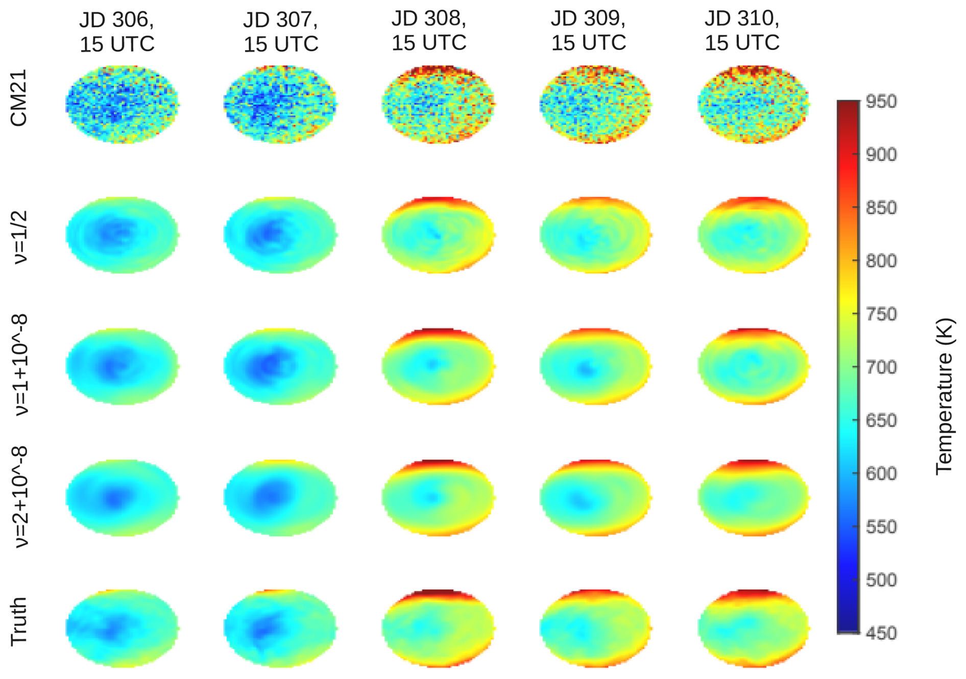
Figure 1 Estimated neutral temperature (first 4 rows) vs simulated field (last row), JD 306-310 at 15:00 UTC (Noon satellite local time) for the model of Cantrall and Matsuo (2021) (top row, CM21) and parameters ν=0.5 (2nd row), $\mathrm{1}+{\mathrm{10}}^{-\mathrm{8}}$ (3rd row), and $\mathrm{2}+{\mathrm{10}}^{-\mathrm{8}}$ (4th row). The algorithm is able to generate accurate estimates of the neutral temperature regardless of the smoothness parameter selected (see Figs. 2 and 3), although the parameter has a noticeable effect on the smoothness of the retrieved field.

As a first pass, we test how our model performs in estimating the neutral temperature at 15:00 UTC, or local noon at satellite nadir. At this time the largest portion of the instrument's viewing area is sunlit, meaning that the algorithm is expected to perform best in this situation. The retrieved fields from JD 306 – JD 310 are shown in Fig. 1, along with the estimates derived using the method of Cantrall and Matsuo (2021) (top row, CM21) and the “true” field from WAM simulations (bottom row). The algorithm closely tracks the true temperature field for all cases, with variations in ν leading to smoother or rougher estimates of the underlying field. It also appears to be much more robust to shot noise than the algorithm of Cantrall and Matsuo (2021).

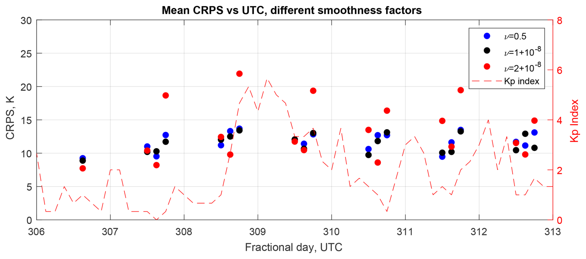
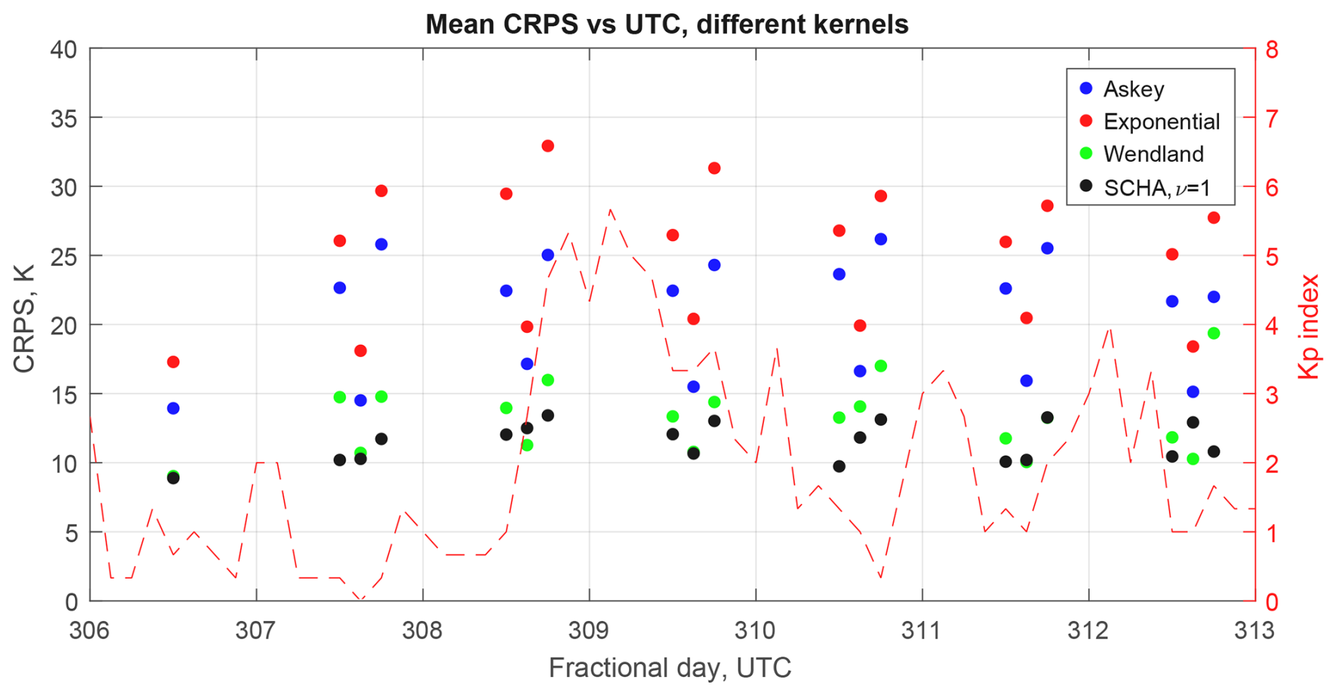
Figure 2 CRPS vs UTC for different kernel smoothness parameters, along with the K_p index from Matzka et al. (2021). The performance of the model depends strongly on local time and decreases slightly during storm time, especially in the case $\mathit{\nu }=\mathrm{2}+{\mathrm{10}}^{-\mathrm{8}}$.

In addition to performance at local noon, we are interested in the performance of our algorithm in low-light conditions. Currently, the GOLD mission does not report TDISK values at an observing zenith angle (OZA) greater than 75° or SZA greater than 80°, which are conservative limits designed to avoid biases in the data products that may arise in these situations (Evans et al., 2024b). This partially motivates our investigation, as we believe that including spatial structure can allow us to obtain accurate estimates of the temperature even at high SZAs. To investigate this, we processed data from 12:00 and 18:00 UTC as well. In this situation, a portion of the viewing area has a solar zenith angle higher than the nominal observation boundary of 80° used by the GOLD mission, however there is still a large portion of the viewing area that is sunlit. At UTC 12:00 and 18:00 approximately 30 % of the viewing area has less than 50 expected counts in the upper band, and about 14 % less than 25. In the lower band, these numbers are about 15 % and 10 % respectively. In this regime, the assumption that counts are Gaussian breaks down, introducing biases and inhibiting uncertainty quantification. Additionally, there are portions of the viewing area where the solar zenith angle exceeds 80° at local noon. These results for the average CRPS at each time are shown in Fig.  2 along with the K_p index. What we see is that the CRPS of the models for ν=0.5 and $\mathit{\nu }=\mathrm{1}+{\mathrm{10}}^{-\mathrm{8}}$ are roughly constant with time and show only a slight increase with the K_p index, never exceeding a CRPS of 15 K. However, the CRPS of the model with $\mathit{\nu }=\mathrm{2}+{\mathrm{10}}^{-\mathrm{8}}$ increases significantly, especially in the afternoon, and exceeds 20 K at 18:00 UTC on JD 308. This is because the onset of even this relatively minor storm generates structure in the field that the model is unable to capture.

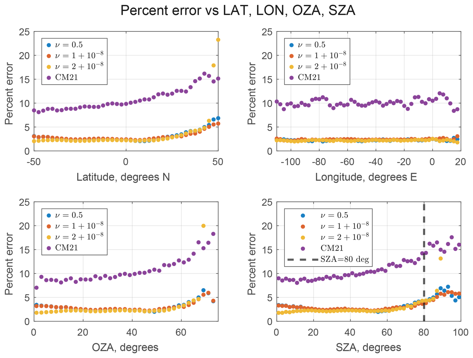
Figure 3 RMS error in percent for varying latitude, longitude, observing angle, and solar zenith angle for the simulated data study. All latitudes and longitudes are included when determining the RMSE as a function of latitude, observing angle, and solar zenith angle, while only latitudes between ±10° are considered when determining the RMSE as a function of longitude.

We have plotted the RMS error in estimation over latitude, longitude, OZA, and SZA in Fig. 3. The permanental process model reduces error by half or more relative to the model of Cantrall and Matsuo (2021) and maintains errors less than 6 % up to nearly 90° SZA. This suggests that the method may be able to extend the scientific utility of FUV disk emission data by allowing analysis of data collected from areas with high SZA.

3.3 Uncertainty Quantification

Our model provides a full posterior distribution of the intensity ratio, and therefore the temperature. In this section, we examine how accurately our model captures uncertainty. This exercise is important to ensure that the model handles uncertainty induced by shot noise properly and that the estimates of the neutral temperature are reliable. We quantify the uncertainty captured by the model by determining the highest posterior density sets with coverage rate r (r-HPD set) for varying values of r. The r-HPD set is the set I_r such that ${\int }_{I_r}f\left(x\right)\mathrm{d}x=r$ and that $\forall \left(x\in I_r,y\in I_r^C\right),f\left(x\right)\ge f\left(y\right)$ (Amaral Turkman et al., 2019). If the posterior distribution accurately quantifies the uncertainty, then the true parameter lies in the r-HPD set with probability r. To determine how well the posterior HPD matches the nominal coverage for varying coverage parameters r, we compare the probability that the true value is within I_r for varying values of r from 0.05 to 0.95. These results are shown in Fig. 4 for the SCHA kernel with $\mathit{\nu }=\mathrm{0.5},\mathrm{1}+{\mathrm{10}}^{-\mathrm{8}},\mathrm{2}+{\mathrm{10}}^{-\mathrm{8}}$, and have been divided into times where K_p<3, indicating calmer conditions, and K_p≥3, indicating higher levels of geomagnetic disturbance.

The coverage probabilities are estimated from 10 retrievals for each simulated field, and then compiled according to K_p index. The plots in Fig. 4 show the median coverage probability over all applicable times and spatial locations from the simulations, and error bars show the 10th and 90th percentiles of coverages. The mean uncertainties at nominal coverage of 0.95 are shown in Table 1 in units of percent of the estimated temperature. Since the intervals are asymmetric, we provide upper and lower uncertainties. The model with ν=0.5 provides the widest uncertainty intervals, and we can see from Fig. 4 that these intervals are too wide, since the achieved coverage greatly exceeds the nominal coverage in all conditions. Practically, this model leads one to believe that estimates of T_eff are more uncertain than they actually are. In a data assimilation scheme, for example, these inflated observation errors can cause the estimated state to artificially biased toward the model, leading to poorly constrained model forecasts. In calm conditions corresponding to a true temperature of 600 K, this model would lead to approximate uncertainties of approximately $(-\mathrm{44},+\mathrm{45})$ K, while the $\mathit{\nu }=\mathrm{1}+{\mathrm{10}}^{-\mathrm{8}}$ model would report uncertainties of about ($-\mathrm{32},+\mathrm{33})$ K and the $\mathit{\nu }=\mathrm{2}+{\mathrm{10}}^{-\mathrm{8}}$ model would report uncertainties of about ±27 K, which Fig. 4 suggests are more accurate representations of the uncertainty due to shot noise. Generally, we see that the $\mathit{\nu }=\mathrm{1}+{\mathrm{10}}^{-\mathrm{8}}$ and $\mathit{\nu }=\mathrm{2}+{\mathrm{10}}^{-\mathrm{8}}$ models appear to be the best at quantifying uncertainty, especially in geomagnetically calm conditions, and their performance degrades in geomagnetically active time periods. The $\mathit{\nu }=\mathrm{2}+{\mathrm{10}}^{-\mathrm{8}}$ model appears especially affected by this transition. This is due to the fact that setting ν higher makes the retrieved field smoother, so it cannot properly recover the structured temperature fields due to geomagnetic disturbances.

Table 1 Average length of 95 % HPD intervals, in units of percent of the temperature estimate, for each value of ν in both calm (K_p<3) and storm (K_p≥3) conditions.

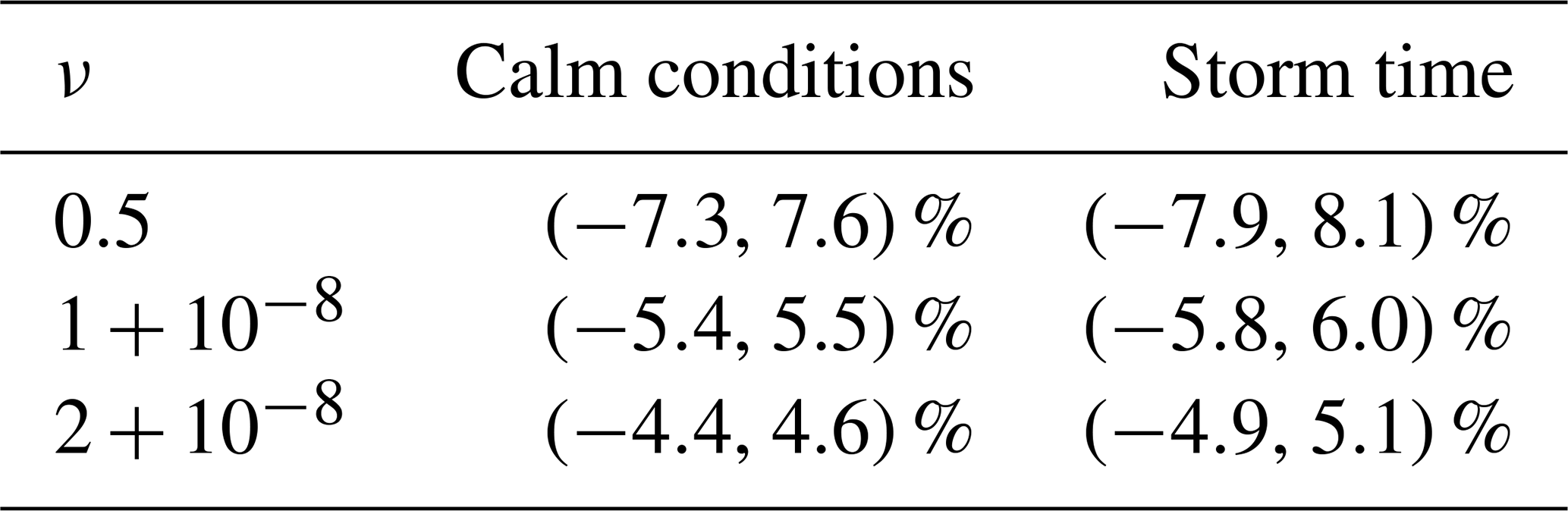
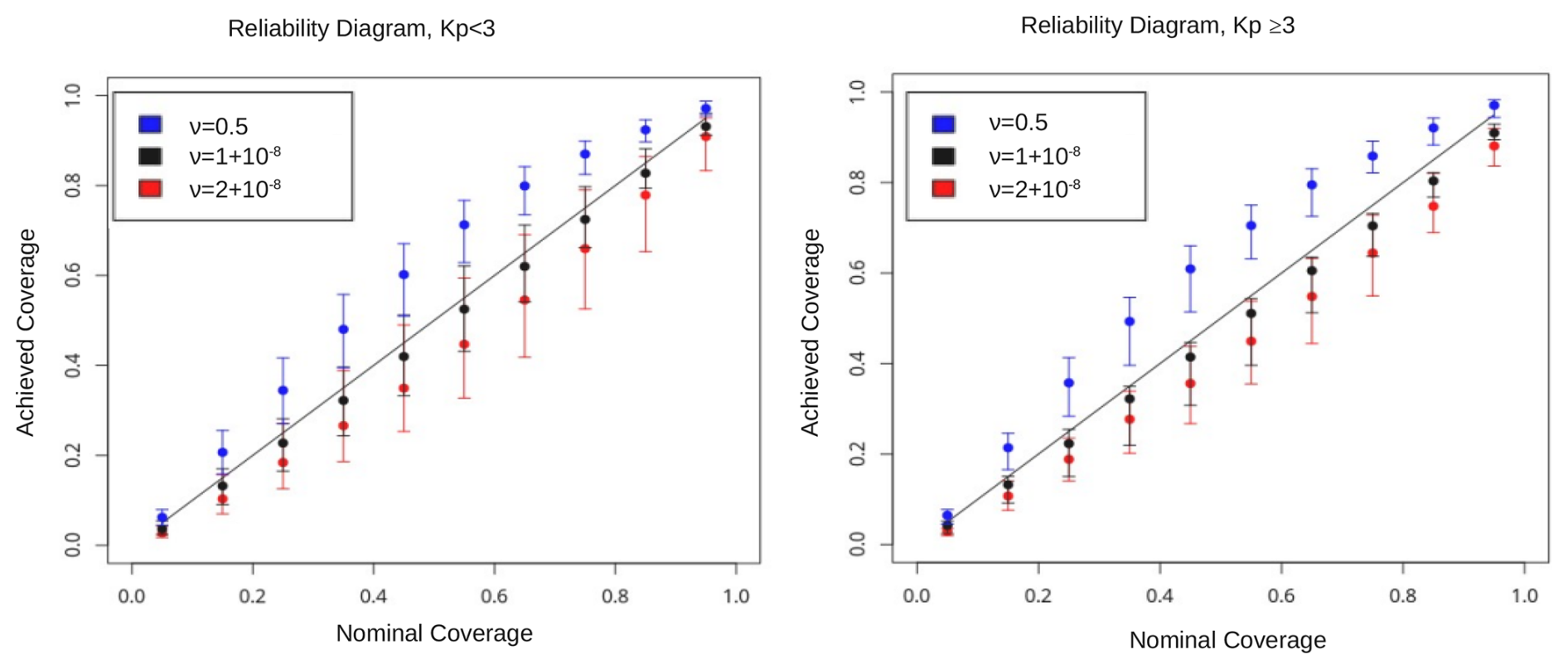
Figure 4 Reliability diagram for the model with varying smoothness parameters and K_p indices. Dots show median coverage probability of a highest-posterior density interval with nominal coverage probability along the x axis, error bars are 10th and 90th percentiles. The models perform worse at uncertainty quantification as K_p increases, however for calm conditions the $\mathit{\nu }=\mathrm{1}+{\mathrm{10}}^{-\mathrm{8}}$ model captures the uncertainty very well.

4 Application to GOLD Disk Emission Data

4.1 November 2018 Geomagnetic Storm

As a first demonstration of the method on real GOLD data, we apply it to background corrected GOLD L1C data from 2–6 November 2018. This is the same time period studied using WAM simulations in Sect. 3, and includes a minor geomagnetic storm on 4–5 November (JD 308-309).

Since the GOLD instrument scans each hemisphere independently, the inversion incorporates two consecutive scans into each retrieval. The start times of these scans are separated in time by 12 min, which is short enough relative to the nominal thermospheric timescales to ignore the time difference between the scans. Since the scans overlap, we average the data in the overlap region, which reduces (but does not completely eliminate) the bias in the retrievals caused by the varying sensitivity of the detector along the slit (Evans et al., 2024b). Again we selected γ=1.

The results of this inversion are shown in Fig. 5. While we obtain similar results to TDISK at high latitudes, as well as on average over SZA and OZA (Fig. 6), there is a visible discrepancy near the equator, corresponding to the lower portion of the scan of the northern hemisphere and the upper portion of the scan of the southern hemisphere. Upon examination of the L1C data, we can see a corresponding enhancement in the count ratio at the same location that is present in the scan of the northern hemisphere, but not the southern hemisphere. This, coupled with the fact that similar artifacts are not seen in the results on simulated data (Fig. 1) suggests that this variation is due to the varying sensitivity of the detector along the slit. Similar artifacts can also be found in earlier versions of the TDISK data (e.g. Fig. 7 of Cantrall and Matsuo, 2021). These artifacts lead to a significant bias in the estimates relative to TDISK at the equator (Fig. 6). It is therefore important to have an understanding of the variations in the detector sensitivity and eliminate artifacts in the retrievals.

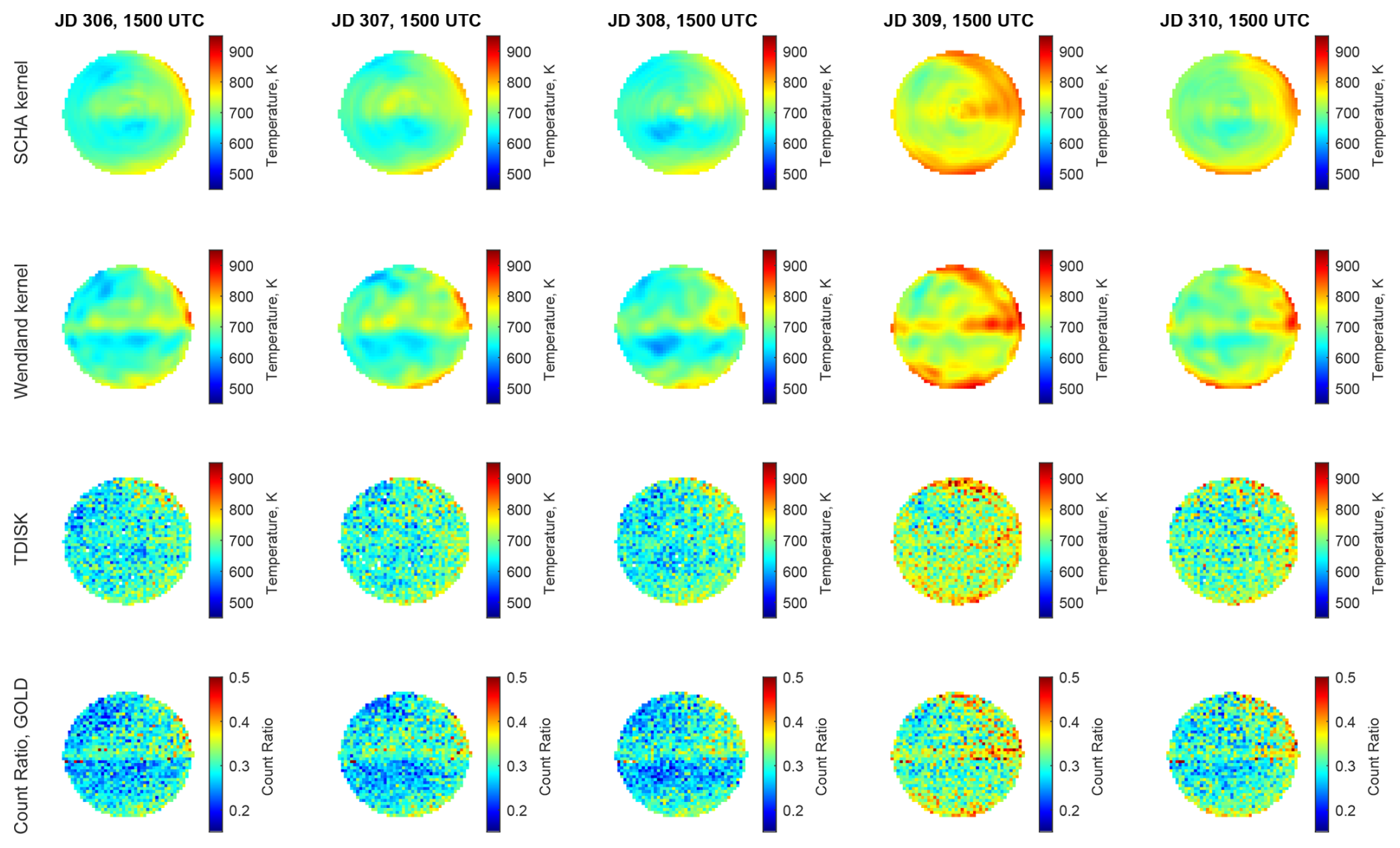
Figure 5 Retrieved temperature using a spherical cap and Wendland kernel (top two rows) compared to TDISK (third row) and the ratio of counts in the upper and lower portion of the LBH (2,0) band (4th row) for JD 306-310, 2018 (2–6 November 2018) at around 15:00 UTC, local noon. The retrieved temperatures contain nonphysical structure near the equator inherited from biases in the data due to differences in the sensitivity of the instrument in the different scans of the equatorial region. Similar artifacts can be seen in older versions of the TDISK data.

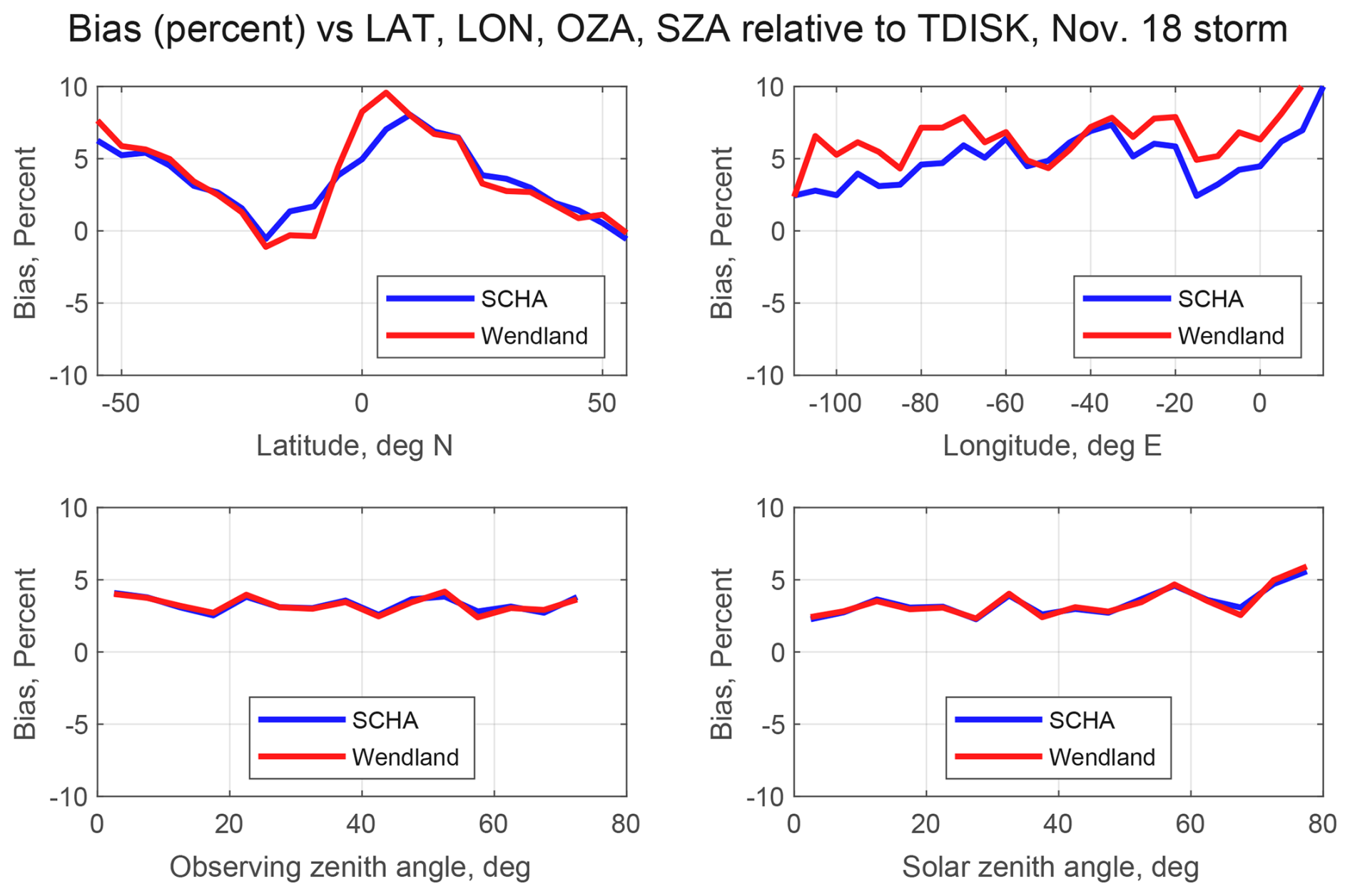
Figure 6 Bias (percent) of estimated temperatures relative to TDISK as a function of latitude, longitude, observing zenith angle, and solar zenith angle during the period of 2–6 November 2018. Our estimates are routinely biased high, in large part due to the variation in detector sensitivity that is not accounted for.

4.2 May 2024 Geomagnetic Storm

The second demonstration example includes a major geomagnetic storm that occurred in May 2024 (also known as the Gannon Storm, Grandin et al., 2024). With the Dst index reaching below −400 nT and a peak K_p index of 9, this storm resulted in a major expansion of the upper atmosphere causing the neutral temperature to elevate, leading to orbital decay of low Earth orbit satellites due to increased atmospheric drag.

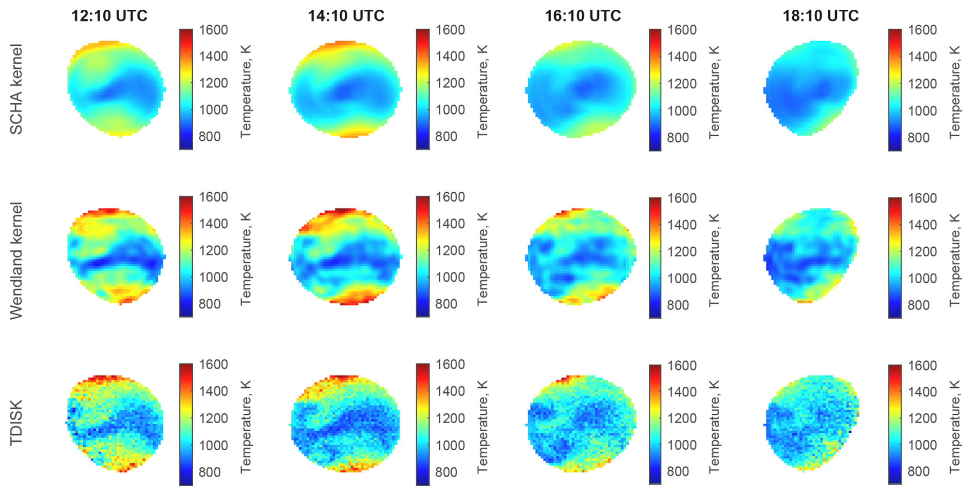
Figure 7 Retrieved temperatures for 12:10–18:10 UTC on 11 May 2024 using both a spherical cap harmonic and Wendland kernel (top two rows) compared with TDISK (bottom row).

The GOLD mission detected previously unseen structure in the thermosphere during this event, simultaneously seen in both LBH and 135.6 nm radiances, as well as retrievals of neutral temperature, atmospheric composition, and total electron content. The detected equator-to-pole differences in neutral temperature of over 400 K, with high-latitude temperatures in excess of 1400 K (Evans et al., 2024a) are well beyond a typical FUV observation and retrieval scenario under nominal conditions. Similar structures have since been observed in other storms as well (Correira et al., 2025). To investigate the performance of our algorithm with the corresponding GOLD L1C data under extreme conditions, we compare our results to the TDISK data product using both the SCHA kernel and a Wendland kernel function given by (Wendland, 1995)

$$\begin{array}{}\text{(17)}& K(d;r)=\left\{\begin{array}{ll}\frac{\mathrm{1}}{\mathrm{3}}{\left(\mathrm{1}-\left|\frac{d}{r}\right|\right)}^{\mathrm{6}}\left(\mathrm{35}{\left|\frac{d}{r}\right|}^{\mathrm{2}}+\mathrm{18}\left|\frac{d}{r}\right|+\mathrm{3}\right),& \left|d\right|<r\\ \mathrm{0},& \left|d\right|\ge r\end{array}\right.\end{array}$$

Note that in the model evaluation with simulated data for November 2018 the Wendland kernel is found to perform similarly to the SCHA kernel, albeit with slightly worse uncertainty quantification (see Appendix C for details). The results of the retrieval for May 2024 are shown in Fig. 7 using $r=\mathrm{1}/\mathrm{3}$ and $\mathit{\nu }=\mathrm{1}+{\mathrm{10}}^{-\mathrm{8}}$ in the Wendland and SCHA kernels respectively. Due to the extreme nature of the storm, we selected a slightly smaller $\mathit{\gamma }=\mathrm{1}/\mathrm{5}$, corresponding to a less informative prior distribution. We see that both models are able to recover spatial structure in the field, especially earlier in the day, however the SCHA kernel tends to oversmooth the estimated field. The retrievals can be improved by more careful selection of the parameters of the kernel, allowing capture of smaller scale structure such as the vortices that are apparent in TDISK, or traveling ionospheric disturbances in more typical scenarios. Our method primarily improves upon Cantrall and Matsuo (2021) by allowing rejection of uncorrelated noise, however small spatial structures can be washed out as well if kernel parameters are not chosen carefully.

We have also included a plot of the relative biases between our two estimates and TDISK during the Gannon storm (Fig. 8). We see that the Wendland kernel results are biased slightly high on average over OZA and SZA, with varying bias with latitude and a low bias at the equator. The SCHA result is generally biased low. The largest bias is less than 8 %, and the average 95 % random uncertainties in TDISK across the plotted estimates are approximately $\mathrm{8.6}\mathit{\%},\mathrm{7.6}\mathit{\%},\mathrm{7.8}\mathit{\%},$ and 8.7 %. The uncertainties in the SCHA and Wendland estimates due to shot noise are approximately ±3 % and ±6 % respectively. The uncertainties from the SCHA appear to be too low, as seen in Fig. 4 when the prior is too smooth. However, using the Wendland kernel leads to uncertainties due to shot noise that are more in line with the estimates provided by TDISK, which incorporate other sources of uncertainty as well (Evans et al., 2024b).

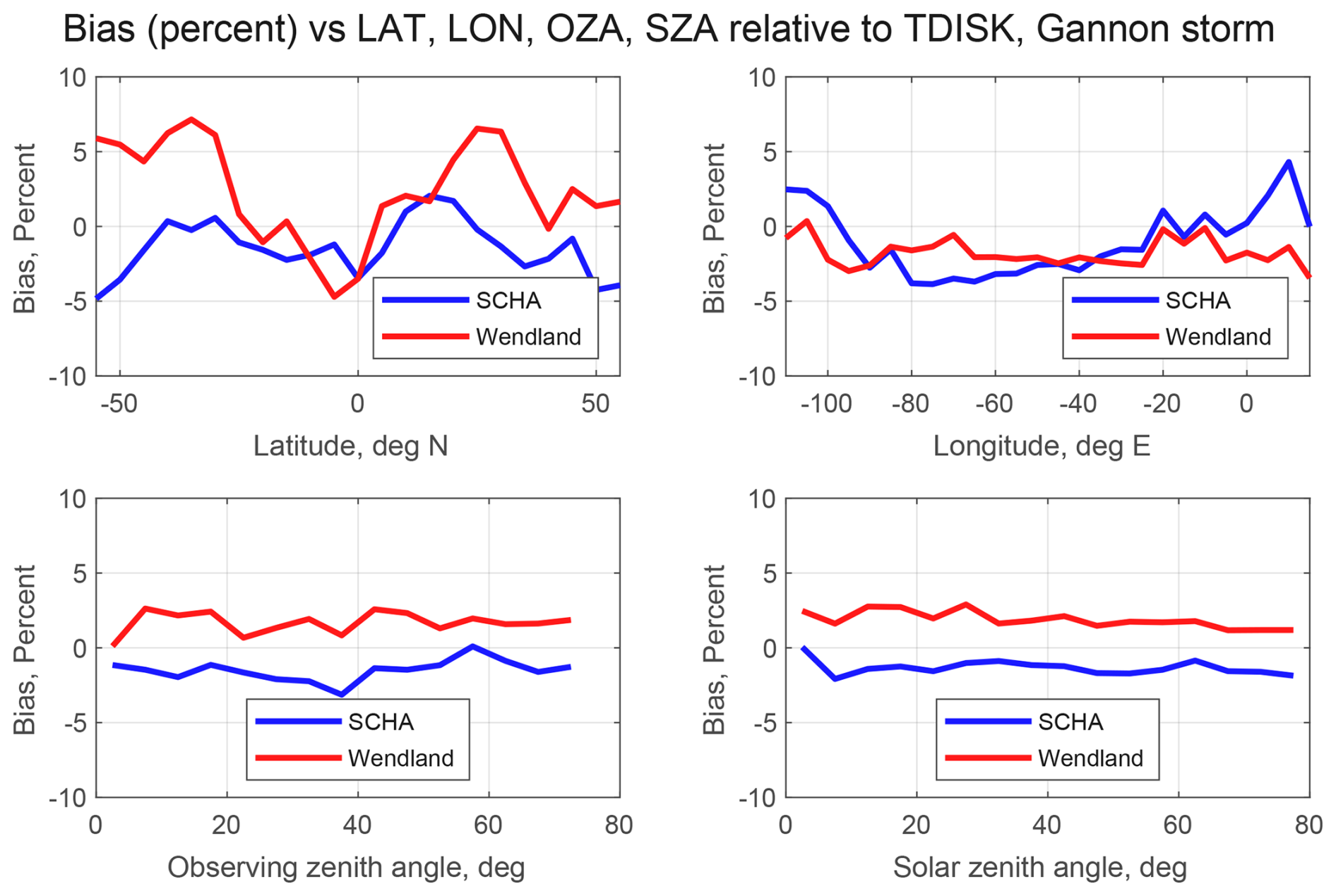
Figure 8 Bias (percent) of estimated temperatures relative to TDISK as a function of latitude, longitude, observing zenith angle, and solar zenith angle during the Gannon storm. Our estimates generally differ from TDISK by less than 5 %, well within the TDISK random uncertainty.

5 Discussion

5.1 Computational Performance

One of the drawbacks of Bayesian methods as practical retrieval algorithms is their computational load. Often, these methods require generating samples from the posterior distribution using an algorithm such as Markov Chain Monte Carlo, which can be computationally expensive. This work overcomes this problem with the use of a closed form approximation to the posterior distribution, shifting the computational load to maximizing the likelihood in Eq. (10). Other options, such as a variational inference approach, are possible (e.g. Lloyd et al., 2015); however, as shown in Walder and Bishop (2017), variational inference is much less efficient than the techniques described in this paper.

The algorithm presented in the previous section is timed on a small runtime analysis study to recover the intensity function:

$$\begin{array}{}\text{(18)}& Z\left(x\right)={\displaystyle \frac{\mathrm{25}\sin {\left(\frac{\mathit{\pi }}{\mathrm{2}}x\right)}^{\mathrm{2}}+\mathrm{10}}{\mathrm{8}\cos {\left(\frac{\mathit{\pi }}{\mathrm{2}}x\right)}^{\mathrm{2}}+\mathrm{10}}},-\mathrm{1}\le x\le \mathrm{1}\end{array}$$

a plot of which is shown in the upper portion of Fig. 9, using logarithmically spaced numbers of bins from 10 to 5600. A Wendland kernel with $r=\mathrm{3}/\mathrm{4}$ is used for the timing study. The minimization is performed with the implementation of conjugate gradient in the optim function in base R using the analytic gradient of Eq. (10) as an input. The results of the timing study are shown in Fig. 9.

With 1500 bins, the average time to retrieve the ratio function is about 40 s on a desktop computer with 16 GB RAM and an Intel i7 CPU. For problems involving less than 500 bins, the algorithm converges in an average of about 3 s, and in about 30 min for problems involving 5600 bins. This suggests that the model can be made fast enough to run in an operational capacity if desired, especially for problems involving data sets in the low to mid thousands of points or less. Due to the eigenvalue decomposition necessary to determine $\stackrel{\mathrm{̃}}{\mathbf{K}}$ the algorithm scales asymptotically as O(n³), which can be mitigated by using a low-rank decomposition, sparse kernel matrices, or precomputing the eigendecomposition of the kernel. Additionally, if the kernel has an explicit Mercer expansion, the need for the eigenvalue decomposition can be avoided altogether. Precomputing the eigendecomposition reduces the runtime for problems involving 1500 bins to about 15 s. The rest of the algorithm does not require any matrix inversions and scales approximately as O(n²). For problems with 1500 bins the peak usage is approximately 2 GB, making it easily small enough to run on commercially available laptops.

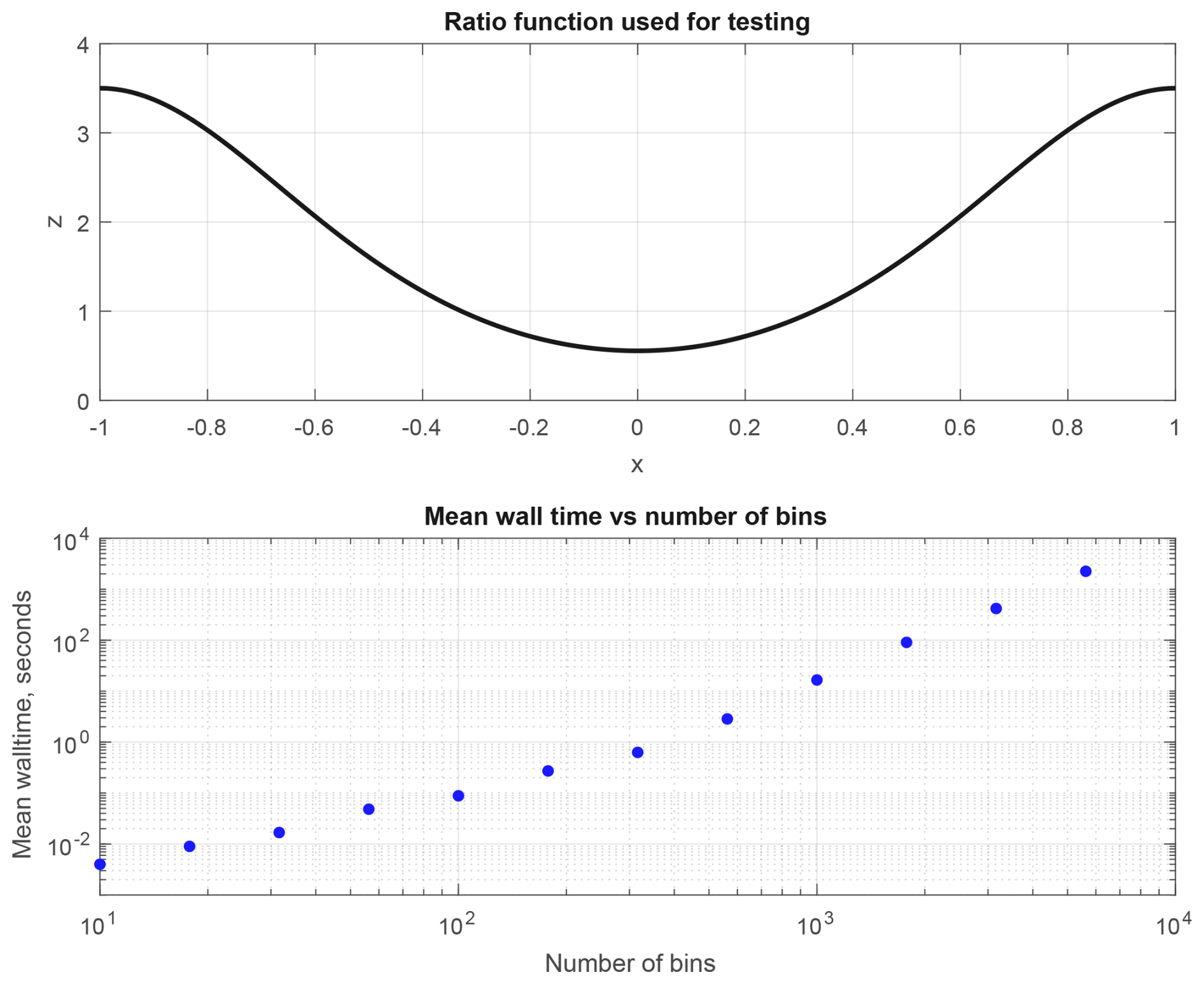
Figure 9 On the top: The ratio function Z(x) estimated in the timing study. On the bottom: timing study results. Times shows are the mean wall times (in s) for the code to execute on a desktop computer over 5 repetitions.

5.2 Future Work

The LBH (1,1) and (2,3) bands are not used in this study in part because they are not considered to have sufficient SNR for temperature retrievals on their own using the two channel ratio method (Cantrall and Matsuo, 2021; Cantrall, 2022). However, both of these bands may be beneficial to consider in the future. While the (2,0) band is not isolated from other LBH emissions, with the lower portion of the band overlapping with the (5,2) band, the (1,1) and (2,3) bands are. This means that, in principle, retrievals using these bands are independent of the specified populations of molecular nitrogen, removing a significant source of model specification error (Cantrall and Matsuo, 2021). Although several works, such as Aryal et al. (2022), Ajello et al. (2020), and Nicholls (1961), have attempted to determine these populations, any errors in the relative populations of the $v^{\prime }=\mathrm{2}$ and $v^{\prime }=\mathrm{5}$ species will contribute to errors in the temperature estimation. For this reason, extending these techniques in a way to allow estimates of the neutral temperature using the (1,1) and (2,3) bands, which have too low of SNR to get accurate T_eff estimates with the band ratio technique (Cantrall and Matsuo, 2021; Cantrall, 2022), or developing a technique that incorporates uncertainty in the vibrational populations may be of interest to practitioners.

One drawback of the two channel ratio method is that it is not robust to wavelength specification errors (Cantrall and Matsuo, 2021; Eastes et al., 2025). This can be partially overcome by using multiple bands, such as the (1,1) and/or (2,3) bands in conjunction with the (2,0) band, to do estimation and weighting observations by their inverse variance, as observed in Cantrall (2022). Under our model the posterior distribution no longer takes on a closed form, being given by the Lauricella D function (Pham-Gia and Turkkan, 2002). One avenue of future research is to determine whether there are suitable approximations to these distributions that would allow incorporation of additional spectral information into the retrieval approach while maintaining efficient computational performance.

One significant advantage of spatial models is the ability to leverage the correlation structure for optimal estimation of the underlying field at unobserved locations, for example via kriging (Stein, 1999). By kriging the latent vector f onto unobserved locations we are able to derive statistically optimal estimates of the neutral temperature at these locations given the model, as well as covariances between observed and unobserved locations. This would allow estimation of the quantity of interest at arbitrary resolution, and additionally allows simulation of spatial fields given observations via conditional simulation (Chiles and Lantuéjoul, 2005). The spatial correlation may also allow estimates of the quantity of interest to be derived without having to perform binning, which is sometimes necessary due to low SNR. The conditions under which such estimation can be done with this model are yet to be studied, but provide a potential avenue for future research.

While we have developed this method with the assumption that the data contain counts generated by a single process, that is not necessarily true. Photons from other sources inhibit retrieval, especially when the source counts are low, and the GOLD instrument's geostationary orbit means it can be subjected to high energy particles from outside sources (Evans et al., 2024b). While the GOLD mission L1C data product used mitigates most of the effect of the background (McClintock et al., 2020), an algorithm that can account for it independently is desirable for further improvement and application to other domains, as uncertainty in the background measurement will necessarily propagate forward into the estimation of the quantity of interest. For instance, the model of Park et al. (2006) handled this by adding a separate term for the background count intensity and estimating both jointly. It is feasible to adopt such an approach to extend this work in the future.

6 Conclusions

While Poisson-distributed multi-spectral sensor data are common in many atmospheric remote sensing applications, current inversion methods used for retrieval of physical parameters often rely on statistical assumptions that may disregard the real statistical properties of sensor data, limiting the scientific utility of datasets. To address this limitation, we introduce a retrieval approach that is based on ratios of photon counts in non-overlapping spectral bands with a focus on FUV upper atmospheric remote sensing applications. This two-channel intensity ratio approach facilitates the development of a computationally efficient and robust method that respects the underlying statistics of the sensor data and naturally incorporates spatial structure. Specifically, the method uses a Poisson point process model with the intensity for each channel independently modeled with a squared Gaussian prior distribution. The new inverse modeling approach is shown to accurately recover spatial structure observed in the true fields and provide a complete posterior distribution of the physical parameter of interest that more faithfully captures variability of underlying geophysical process. The approach is demonstrated on thermospheric neutral temperature retrievals from simulated top-of-atmosphere FUV disk emission data during a minor geomagnetic storm period in November 2018, and from actual calibrated disk emission (L1C) data from the GOLD mission for the same period as well as a major geomagnetic storm that occurred in May 2024. We show that the overall features of retrieved column-integrated temperature are generally consistent with the GOLD mission (TDISK v5) data product and demonstrate the potential for providing reliable uncertainty quantification, as well as enabling retrieval of thermospheric neutral temperature in low-SNR scenarios, including at extremely high solar zenith angles.

Appendix A: Derivation of Eq. (4)

In Eq. (4), we present without proof the posterior distribution of the intensity ratio in the case of pointwise inversion with no background, as done in Jin et al. (2006) and Park et al. (2006), as a BP($\mathit{\alpha },\mathit{\beta },p,q)$ distribution. This model contains as a special case priors of the form $x^{-k_i}$, equivalent to ${\mathit{\alpha }}_i=\mathrm{1}-k_i$ and β_i=0. The proofs for the cases $n_a=n_b=\mathrm{1}$ with $k_a=k_b=\mathrm{0}$ and $k_a=k_b=\mathrm{0.5}$ are given in Jin et al. (2006), but the distributions are not named as the $BP(a+\mathrm{1}-k_a,b+\mathrm{1}-k_b,\mathrm{1},\mathrm{1})$ distribution.

Assume that the count data $\mathit{\{}{a}_i{\mathit{\}}}_{i=\mathrm{1}}^{n_a}$ from the upper channel and $\mathit{\{}{b}_i{\mathit{\}}}_{i=\mathrm{1}}^{n_b}$ from the lower channel are independent with

$$\begin{array}{l}{\displaystyle }{a}_i|{\mathrm{\Lambda }}_a\stackrel{\mathrm{iid}}{\sim }\text{Poisson}\left({\mathrm{\Lambda }}_a\right)\\ {\displaystyle }{b}_i|{\mathrm{\Lambda }}_b\stackrel{\mathrm{iid}}{\sim }\text{Poisson}\left({\mathrm{\Lambda }}_b\right)\end{array}$$

for all i, where n_a and n_b are the number of independent observations of the total counts in each channel. In the case of GOLD data where we do 2x2 spatial binning prior to processing, $n_a=n_b=\mathrm{4}$. Now consider the prior ${\mathrm{\Lambda }}_i\sim \mathrm{\Gamma }({\mathit{\alpha }}_i,{\mathit{\beta }}_i)$ for each Λ_i. Let $a={\sum }_{i=\mathrm{1}}^{n_a}{a}_i$ and $b={\sum }_{i=\mathrm{1}}^{n_b}{b}_i$. Then since the Gamma distribution is the conjugate prior of Λ we have that ${\mathrm{\Lambda }}_a\sim \mathrm{\Gamma }(a+{\mathit{\alpha }}_a,{\mathit{\beta }}_a+n_a)$ and ${\mathrm{\Lambda }}_b\sim \mathrm{\Gamma }(b+{\mathit{\alpha }}_b,{\mathit{\beta }}_b+n_b)$.

So, the intensity ratio $Z=\frac{{\mathrm{\Lambda }}_a}{{\mathrm{\Lambda }}_b}$ has the distribution

$$\begin{array}{}\text{(A1)}& \begin{array}{rl}\mathbb{P}\left[Z\le z\right]& =\mathbb{P}\left[{\displaystyle \frac{{\mathrm{\Lambda }}_a}{{\mathrm{\Lambda }}_b}}\le z\right]=\underset{\mathrm{0}}{\overset{\mathrm{\infty }}{\int }}\mathbb{P}\left[{\displaystyle \frac{{\mathrm{\Lambda }}_a}{{\mathrm{\Lambda }}_b}}\le z|{\mathrm{\Lambda }}_b=x\right]\\ & \text{d}\mathbb{P}\left[{\mathrm{\Lambda }}_b=x\right]\\ & =\underset{\mathrm{0}}{\overset{\mathrm{\infty }}{\int }}\mathbb{P}\left[{\mathrm{\Lambda }}_a\le z{\mathrm{\Lambda }}_b|{\mathrm{\Lambda }}_b=x\right]\text{d}\mathbb{P}\left[{\mathrm{\Lambda }}_b=x\right]\\ & ={\displaystyle \frac{({\mathit{\beta }}_a+n_a{)}^{a+{\mathit{\alpha }}_a}({\mathit{\beta }}_b+n_b{)}^{b+{\mathit{\alpha }}_b}}{\mathrm{\Gamma }(a+{\mathit{\alpha }}_a)\mathrm{\Gamma }(b+{\mathit{\alpha }}_b)}}\underset{\mathrm{0}}{\overset{\mathrm{\infty }}{\int }}\\ & \left[\underset{\mathrm{0}}{\overset{zx}{\int }}{y}^{a+{\mathit{\alpha }}_a-\mathrm{1}}{e}^{-({\mathit{\beta }}_a+n_a)y}\text{d}y\right]\\ & x^{b+{\mathit{\alpha }}_b-\mathrm{1}}{e}^{-({\mathit{\beta }}_b+n_b)x}\text{d}x\end{array}\end{array}$$

The integrand is differentiable in z and is an ℒ¹ function in x, so by Lebesgue's Dominated Convergence Theorem we can pass derivatives into the integral. Then the probability density is given by

$$\begin{array}{}\text{(A2)}& \begin{array}{rl}{p}_Z\left(z\right)& ={\displaystyle \frac{({\mathit{\beta }}_a+n_a{)}^{a+{\mathit{\alpha }}_a}({\mathit{\beta }}_b+n_b{)}^{b+{\mathit{\alpha }}_b}}{\mathrm{\Gamma }(a+{\mathit{\alpha }}_a)\mathrm{\Gamma }(b+{\mathit{\alpha }}_b)}}\underset{\mathrm{0}}{\overset{\mathrm{\infty }}{\int }}{\displaystyle \frac{\partial }{\partial z}}\\ & \left[\underset{\mathrm{0}}{\overset{zx}{\int }}{y}^{a+{\mathit{\alpha }}_a-\mathrm{1}}{e}^{-({\mathit{\beta }}_a+n_a)y}\text{d}y\right]x^{b+{\mathit{\alpha }}_b-\mathrm{1}}{e}^{-({\mathit{\beta }}_b+n_b)x}\text{d}x\\ & ={\displaystyle \frac{({\mathit{\beta }}_a+n_a{)}^{a+{\mathit{\alpha }}_a}({\mathit{\beta }}_b+n_b{)}^{b+{\mathit{\alpha }}_b}}{\mathrm{\Gamma }(a+{\mathit{\alpha }}_a)\mathrm{\Gamma }(b+{\mathit{\alpha }}_b)}}\\ & \underset{\mathrm{0}}{\overset{\mathrm{\infty }}{\int }}{x}^{a+b+{\mathit{\alpha }}_a+{\mathit{\alpha }}_b-\mathrm{1}}{e}^{-({\mathit{\beta }}_b+n_b+({\mathit{\beta }}_a+n_a\left)z\right)x}\text{d}x\end{array}\end{array}$$

Letting $t=({\mathit{\beta }}_b+n_b+({\mathit{\beta }}_a+n_a\left)z\right)x$ we see that

$$\begin{array}{}\text{(A3)}& \begin{array}{rl}{p}_Z\left(z\right)& ={\displaystyle \frac{({\mathit{\beta }}_a+n_a{)}^{a+{\mathit{\alpha }}_a}({\mathit{\beta }}_b+n_b{)}^{b+{\mathit{\alpha }}_b}}{\mathrm{\Gamma }(a+{\mathit{\alpha }}_a)\mathrm{\Gamma }(b+{\mathit{\alpha }}_b)}}\\ & \underset{\mathrm{0}}{\overset{\mathrm{\infty }}{\int }}{x}^{a+b+{\mathit{\alpha }}_a+{\mathit{\alpha }}_b-\mathrm{1}}{e}^{-({\mathit{\beta }}_b+n_b+({\mathit{\beta }}_a+n_a\left)z\right)x}\text{d}x\\ & ={\displaystyle \frac{\mathrm{1}}{B(a+{\mathit{\alpha }}_a,b+{\mathit{\beta }}_b)}}{\displaystyle \frac{{\left(\frac{{\mathit{\beta }}_a+n_a}{{\mathit{\beta }}_b+n_b}\right)}^{a+{\mathit{\alpha }}_a}{z}^{a+{\mathit{\alpha }}_a-\mathrm{1}}}{{\left(\mathrm{1}+\frac{{\mathit{\beta }}_a+n_a}{{\mathit{\beta }}_b+n_b}z\right)}^{a+b+{\mathit{\alpha }}_a+{\mathit{\alpha }}_b}}}\end{array}\end{array}$$

which is a $BP(a+{\mathit{\alpha }}_a,b+{\mathit{\alpha }}_b,\mathrm{1},\frac{{\mathit{\beta }}_b+n_b}{{\mathit{\beta }}_a+n_a})$ distribution as desired.

Appendix B: Derivation of the Posterior Mean and Covariance from Eq. (10)

From Eq. (10) we know that

$$\mathrm{\ell }\left(\mathit{\psi }\right|\mathit{\left\{}{a}_i{\mathit{\}}}_{i=\mathrm{1}}^d\right)=\sum _{i=\mathrm{1}}^d{a}_i\log \left({\displaystyle \frac{c}{\mathrm{2}}}{\left(\stackrel{\mathrm{̃}}{\mathbf{K}}\mathit{\psi }\right)}_i^{\mathrm{2}}\right)-{\displaystyle \frac{\mathrm{1}}{\mathrm{2}}}{\mathit{\psi }}^T\stackrel{\mathrm{̃}}{\mathbf{K}}\mathit{\psi }$$

In order to derive the posterior mean and covariance, we will first write f=Φ^Tβ. Then the likelihood becomes

$$\begin{array}{}\text{(B1)}& \mathrm{\ell }\left(\mathit{\alpha }\right|\mathit{\left\{}{a}_i{\mathit{\}}}_{i=\mathrm{1}}^d\right)=\sum _{i=\mathrm{1}}^d{a}_i\log \left({\displaystyle \frac{c}{\mathrm{2}}}{\left({\mathbf{\Phi }}^T\mathit{\beta }\right)}_i^{\mathrm{2}}\right)-{\displaystyle \frac{\mathrm{1}}{\mathrm{2}}}〈\mathit{\beta },\left(c\mathbf{I}+\mathit{\gamma }{\mathbf{H}}^{-\mathrm{1}}\right)\mathit{\beta }〉\end{array}$$

where H=diag(η_i). From this we can see that the posterior mode estimate of β must satisfy

$$\begin{array}{}\text{(B2)}& \begin{array}{rl}\widehat{\mathit{\beta }}& ={\left(c\mathbf{I}+\mathit{\gamma }{\mathbf{H}}^{-\mathrm{1}}\right)}^{-\mathrm{1}}{\mathrm{\nabla }}_{\mathit{\beta }}\left[\sum _{i=\mathrm{1}}^d{a}_i\log \left({\displaystyle \frac{c}{\mathrm{2}}}{\left({\mathbf{\Phi }}^T\widehat{\mathit{\beta }}\right)}_i^{\mathrm{2}}\right)\right]\\ & ={\left(c\mathbf{I}+\mathit{\gamma }{\mathbf{H}}^{-\mathrm{1}}\right)}^{-\mathrm{1}}\sum _{i=\mathrm{1}}^d{\displaystyle \frac{\mathrm{2}{a}_i{\mathbf{\Phi }}_{:,i}}{{\left({\mathbf{\Phi }}^T\widehat{\mathit{\beta }}\right)}_i}}\end{array}\end{array}$$

where ${\mathbf{\Phi }}_{:,i}$ is the ith column of Φ. Then the posterior mode estimate of f is then given by

$$\begin{array}{}\text{(B3)}& \widehat{\mathit{f}}={\mathbf{\Phi }}^T\widehat{\mathit{\beta }}=\sum _{i=\mathrm{1}}^d\left[{\mathbf{\Phi }}^T{\left(c\mathbf{I}+\mathit{\gamma }{\mathbf{H}}^{-\mathrm{1}}\right)}^{-\mathrm{1}}{\mathbf{\Phi }}_{:,i}\right]{\displaystyle \frac{\mathrm{2}{a}_i}{{\left({\mathbf{\Phi }}^T\widehat{\mathit{\beta }}\right)}_i}}\end{array}$$

From this, we can see the posterior mode has the form $\widehat{\mathit{f}}=\stackrel{\mathrm{̃}}{\mathbf{K}}\widehat{\mathit{\psi }}$ by applying the eigenvector expansion of $\stackrel{\mathrm{̃}}{\mathbf{K}}$. This implies that, in our situation, ${\widehat{\mathit{\psi }}}_i=\frac{\mathrm{2}{a}_i}{\widehat{{\mathit{f}}_i}}$, which is analogous to Eq. (11) in Walder and Bishop (2017). This posterior mode is used as the posterior mean in the Laplace approximation of the posterior distribution.

The inverse of the posterior covariance of β is given by the Hessian matrix at the posterior mode, given by

$$\begin{array}{}\text{(B4)}& \begin{array}{rl}{\mathbf{Q}}^{-\mathrm{1}}& =-{\displaystyle \frac{{\partial }^{\mathrm{2}}}{\partial \mathit{\beta }\partial {\mathit{\beta }}^T}}L\left(\mathit{\beta }\right|\mathit{\left\{}{a}_j{\mathit{\}}}_{j=\mathrm{1}}^d\right){|}_{\widehat{\mathit{\beta }}}=\left(c\mathbf{I}+\mathit{\gamma }{\mathbf{H}}^{-\mathrm{1}}\right)\\ & +\sum _{i=\mathrm{1}}^d{\displaystyle \frac{\mathrm{2}{a}_i}{{\left({\mathbf{\Phi }}^T\widehat{\mathit{\beta }}\right)}_i^{\mathrm{2}}}}{\mathbf{\Phi }}_{:,i}{\mathbf{\Phi }}_{:,i}^T\end{array}\end{array}$$

Now letting $\mathbf{Z}=\left(c\mathbf{I}+\mathit{\gamma }{\mathbf{H}}^{-\mathrm{1}}\right)$ and $\mathbf{D}=\text{diag}\left(\frac{{\widehat{\mathit{\psi }}}_j^{\mathrm{2}}}{\mathrm{2}{a}_j}\right)$ we have that ${\mathbf{Q}}^{-\mathrm{1}}=\mathbf{Z}+\mathbf{\Phi }\mathbf{D}{\mathbf{\Phi }}^T$ and can apply the Woodbury-Morrison formula to write that

$$\begin{array}{}\text{(B5)}& \mathbf{Q}={\mathbf{Z}}^{-\mathrm{1}}-{\mathbf{Z}}^{-\mathrm{1}}\mathbf{\Phi }{\left({\mathbf{D}}^{-\mathrm{1}}+{\mathbf{\Phi }}^T{\mathbf{Z}}^{-\mathrm{1}}\mathbf{\Phi }\right)}^{-\mathrm{1}}{\mathbf{\Phi }}^T{\mathbf{Z}}^{-\mathrm{1}}\end{array}$$

The posterior covariance matrix of f is then given by

$$\begin{array}{}\text{(B6)}& {\displaystyle }\widehat{\mathbf{\Sigma }}& {\displaystyle }={\mathbf{\Phi }}^T\mathbf{Q}\mathbf{\Phi }\text{(B7)}& {\displaystyle }& {\displaystyle }=\stackrel{\mathrm{̃}}{\mathbf{K}}-\stackrel{\mathrm{̃}}{\mathbf{K}}{\left({\mathbf{D}}^{-\mathrm{1}}+\stackrel{\mathrm{̃}}{\mathbf{K}}\right)}^{-\mathrm{1}}\stackrel{\mathrm{̃}}{\mathbf{K}}\end{array}$$

as desired.

Appendix C: The kernel

Since we wish to retrieve a field whose domain is the surface of the sphere, one option for constructing the eigenvector expansion of the kernel would be to use spherical harmonics. However, since we are only observing a portion of the sphere this would mean that the underlying intensity field is assumed to be 0 outside the viewing area and so is not continuous. Thus, using spherical harmonics, which are nonlocalized analytic functions, to represent the field can lead to nonphysical ringing in the retrieved fields. Instead, we choose the expansion of the kernel to be given in terms of spherical cap harmonics V_lm (SCHAs, Haines, 1985). These functions form an orthonormal basis for the Hilbert space of square integrable functions on the spherical cap, making them a natural basis for this problem. They have been used extensively in geoscience, for example in determining electrodynamics of the polar ionosphere (Richmond and Kamide, 1988), statistical analysis of TOPEX/POSEIDON data (Hwang and Chen, 1997), and mapping of total electron content over China and Iran (Liu et al., 2011; Razin and Voosoghi, 2017).

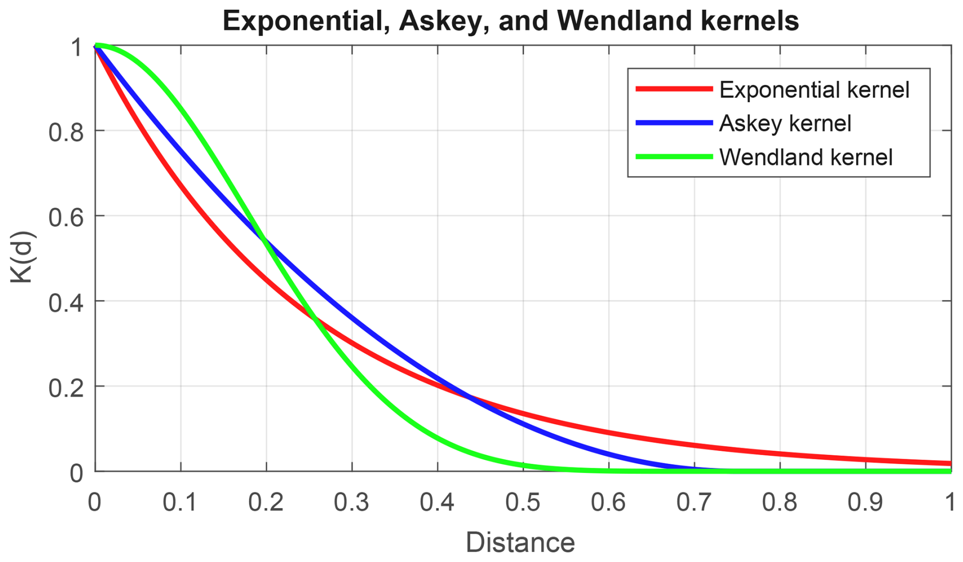
Figure C1 Askey (blue), exponential (red) and Wendland (green) kernels. The Askey and exponential kernels give rise to a rough process, while the Wendland kernel gives rise to a smoother process.

Figure C2 CRPS vs time for the Askey, exponential, Wendland, and SCHA kernels.

There are two families of spherical cap harmonics. One is the so-called even harmonics, which are calculated by solving the eigenvalue problem (Haines, 1985)

$$\begin{array}{}\text{(C1)}& \begin{array}{rl}\mathrm{\Delta }{V}_{lm}(\mathit{\theta },\mathit{\varphi })& ={\displaystyle \frac{\mathrm{1}}{{\mathit{\eta }}_{lm}}}{V}_{lm}(\mathit{\theta },\mathit{\varphi })\\ V_{lm}(\mathit{\theta },\mathit{\varphi })& =V_{lm}(\mathit{\theta },\mathit{\varphi }+\mathrm{2}\mathit{\pi })\\ {\displaystyle \frac{\partial }{\partial \mathit{\varphi }}}{V}_{lm}(\mathit{\theta },\mathit{\varphi })& ={\displaystyle \frac{\partial }{\partial \mathit{\varphi }}}{V}_{lm}(\mathit{\theta },\mathit{\varphi }+\mathrm{2}\mathit{\pi })\\ {\displaystyle \frac{\partial }{\partial \mathit{\theta }}}{V}_{lm}({\mathit{\theta }}_{\mathrm{0}},\mathit{\varphi })& =\mathrm{0}\\ V_{lm}(\mathrm{0},\mathit{\varphi })& =\mathrm{0}\text{, }m=\mathrm{0}\\ {\displaystyle \frac{\partial }{\partial \mathit{\theta }}}{V}_{lm}(\mathrm{0},\mathit{\varphi })& =\mathrm{0},m\ne \mathrm{0}\end{array}\end{array}$$

where θ₀ is the co-latitude of the cap boundary, taken for our purposes to be 64°. The odd harmonics are retrieved when the boundary condition $\frac{\partial }{\partial \mathit{\theta }}{V}_{lm}({\mathit{\theta }}_{\mathrm{0}},\mathit{\varphi })=\mathrm{0}$ is replaced by $V_{lm}({\mathit{\theta }}_{\mathrm{0}},\mathit{\varphi })=\mathrm{0}$. The even harmonics allow for the reconstruction of an arbitrary function on the boundary, and the odd harmonics allow reconstruction of a field with an arbitrary derivative at the boundary. Each of these sets of functions form an orthonormal basis of ℒ²(S), however they are not mutually orthogonal. Since we are concerned with reconstruction of the temperature field and not its derivatives, we choose to represent the field with the even harmonics. The solutions to this problem are the eigenvalue/eigenfunction pairs

$$\begin{array}{}\text{(C2)}& \begin{array}{rl}{V}_{lm}(\mathit{\theta },\mathit{\varphi })& =e^{im\mathit{\varphi }}{P}_{lm}\left(\cos \right(\mathit{\theta }\left)\right)\\ {\mathit{\eta }}_{lm}& ={\displaystyle \frac{\mathrm{1}}{l(l+\mathrm{1})}}\end{array}\end{array}$$

where P_lm are the associated Legendre functions, and l need not be an integer, but m∈ℤ and $l>\left|m\right|$. The associated Legendre functions are not polynomials, but instead are related to the hypergeometric function (Hwang and Chen, 1997). Due to the computational difficulty of solving the eigenvalue problem for various l,m we only calculate the SCHAs up to m=20, corresponding to 441 basis functions. Thus, the kernel K is given by Eq. (15), and the equivalent kernel is then given by

$$\begin{array}{}\text{(C3)}& {\stackrel{\mathrm{̃}}{\mathbf{K}}}_{ij}=\sum _{l,m}{\displaystyle \frac{\mathrm{1}}{c+\mathit{\gamma }{l}^{\mathit{\nu }}(\mathrm{1}+l{)}^{\mathit{\nu }}}}{V}_{lm}({\mathit{\theta }}_i,{\mathit{\varphi }}_i)V_{lm}\left({\mathit{\theta }}_j,{\mathit{\varphi }}_j\right)\end{array}$$

Figure C3 Reliability diagram for the different kernels, all K_p values.

As was shown in the body of the paper, the best of the SCHA kernels studied in terms of uncertainty quantification and retrieval accuracy was the one where $\mathit{\nu }=\mathrm{1}+{\mathrm{10}}^{-\mathrm{8}}$. We will compare this specific kernel with several other popular kernels that are positive definite on the sphere. A list of some possible kernels is included in Gneiting (2013). We choose to compare the SCHA kernel to the Askey kernel, given by

$$\begin{array}{}\text{(C4)}& K(d;r)=\left\{\begin{array}{ll}{\left(\mathrm{1}-\left|\frac{d}{r}\right|\right)}^{\mathrm{2}}& \left|d\right|<r\\ \mathrm{0}& \left|d\right|\ge r,\end{array}\right.\end{array}$$

the exponential kernel, given by

$$\begin{array}{}\text{(C5)}& K(d;r)=\exp \left(-\left|{\displaystyle \frac{d}{r}}\right|\right),\end{array}$$

and the Wendland kernel given by Eq. (17). These kernels are plotted in Fig. C1. In all cases, the distance measure is the angular distance. From this figure, we see one feature that separates the Wendland from the other kernels: the number of derivatives that a kernel function has at d=0 is related to the number of mean-square derivatives of the field (Stein, 1999), and the Askey and exponential kernels do not have any derivatives at d=0, while the Wendland kernel does. This suggests that the Wendland kernel will generate smoother fields than the other two. Additionally, the Askey and Wendland kernels are compactly supported, meaning that they give rise to sparse kernel matrices. This property could make them useful in the analysis of large datasets, where correlations being zero outside a cutoff distance means that the algorithm can take advantage of sparsity in the resulting matrices. The exponential kernel is the covariance of an AR-1 process, leading to a sparse precision matrix for f.

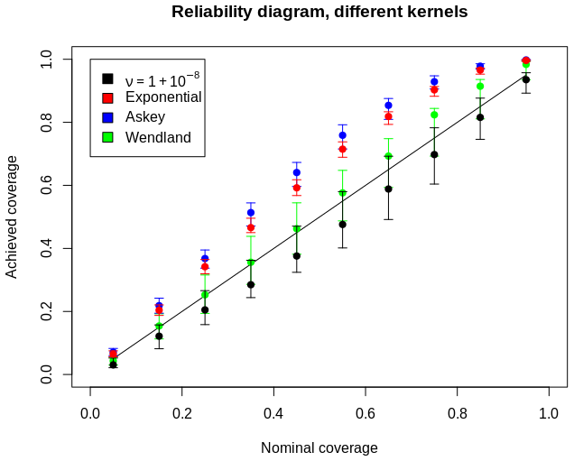
We performed temperature retrievals on the simulated data examined in Sect. 3. In general, we found that the Wendland kernel had similar retrieval performance in terms of CRPS, with slightly worse uncertainty quantification as the nominal coverage increases. The other two kernels were not competitive in either metric. These results are shown in Figs. C2 and C3. We expect that this is due to the implied roughness of the fields from the Askey and exponential kernels. Since the retrieved field is an integrated quantity, we expect it to be relatively smooth, and from the data we see that in most conditions it is. This makes the Askey and exponential kernels less appropriate for the retrieval and less accurate in quantifying the uncertainty. The SCHA kernel with ν=0.5 showed similar levels of overdispersion in the posterior distribution, suggesting that incorrectly specifying the smoothness of the field is to blame.

While these results show that the SCHA kernel is the best option for our analysis on the simulated data, we want to stress that any operational choice of kernel should involve careful cross-validation and other thorough testing before use. This is especially important because the application of the SCHA kernel to time periods where most of the disk is not illuminated could cause problems akin to the ringing issue experienced with spherical harmonics. In a situation like this, a Wendland kernel or another one not investigated here may be preferable. In fact, we see already in Sect. 4 that in the case of the Gannon storm a Wendland kernel is preferable to the SCHA kernel.