Characterisation of spectroscopic properties of DOAS instruments using high-resolution solar spectra

The characterisation of spectroscopic properties of DOAS instruments is important for accurate trace gas retrievals. In this study, we investigate and extend existing methods for the determination of spectroscopic properties using high-resolution solar spectra (also known as Kurucz fit, KF, approaches). We apply these methods to long-term zenith-sky DOAS measurements in Kiruna (northern Sweden). This unique data set allows to study the performance and precision of such fitting procedures under different environmental and observational conditions. Also, the effect of the change of the detector from a photodiode array to a modern CCD is investigated. One key finding of our study is that the so-called Ring effect (caused by rotational Raman scattering) leads to a systematic broadening (by typically about 10 %) of the width of the instrument spectral response function (ISRF) derived from a KF compared to the true ISRF derived from atomic line lamp measurements. Especially for measurements of trace gases located close to the ground this broadening can lead to errors of the trace gas results if a KF-derived ISRF is used for the preparation of trace gas reference spectra and Ring spectra. Here it is important that the strength of the Ring effect can strongly change due to clouds, in particular in the presence of optically thick clouds. Measurements in the presence of optically thick clouds should thus not be chosen for the application of the KF. Another specific finding for the Kiruna measurements (also relevant for other high latitude stations) is that the Ring effect changes systematically with season because of the changing surface albedo (caused by snow cover in the winter). From KF, different instrument properties can be obtained. We give specific recommendations for different KF variants for the determination of the ISRF, intensity offsets (e.g. caused by spectrograph straylight), or the wavelength dependence of the light throughput of the instrument. We also show that a strong wavelength dependence of the light throughput (e.g. caused by the Fabry–Pérot etalon effect) can lead to wrong trace gas results. This finding might also be relevant for other instruments affected by strong Fabry–Pérot etalon effects, or containing other optical elements with strong wavelength-dependent light throughputs. Finally, we introduce a method to correct such a wavelength-dependent light throughput using the results of a modified KF.

1 Introduction

The exact knowledge of the spectroscopic properties of a DOAS (Differential Optical Absorption Spectroscopy) instrument (Platt and Stutz, 2008) is crucial for the correct analysis of atmospheric trace gases, in particular for weak absorbers with optical depths of about 0.1 % or below. Probably the most important spectroscopic property is the so-called instrumental spectral response function (ISRF), frequently referred to as “slit function”. Other important properties are the light throughput and the straylight level (and their wavelength dependencies), or the spectral sampling (i.e. the number of detector pixels per wavelength). Information on these properties is usually provided by the instrument manufacturer or can be determined from dedicated measurements in the laboratory. However, such measurements are often difficult to perform and analyse (and typically require extra hardware like wavelength calibration lamps), and – probably more important – the determined spectroscopic properties often change via transport from the laboratory to the field. Such problems can be avoided by the determination of the spectroscopic properties from the routine measurements of a DOAS instrument. From the comparison (usually by a fitting procedure) of the measured spectra of (scattered) sun light to a high-resolution catalog (e.g. from Kurucz et al., 1984), the spectroscopic properties can be continuously monitored during operation of the instrument in the field. As another advantage, potential effects of different illumination of the spectrometer grating by the calibration lamps and the atmospheric measurements are avoided. Continuous monitoring of the spectroscopic properties of DOAS instruments from routine measurements is especially important for trend studies to make sure that the retrieved trends are not introduced by instrumental artefacts.

The characterisation of the ISRF and the pixel to wavelength assignment derived from fits to high-resolution solar spectra is a well-established technique (Fayt and Roozendael, 2001; Aliwell et al., 2002; Danckaert et al., 2017). Often these fits are referred to as “Kurucz procedure” or “Kurucz fit” (KF), because the high-resolution solar spectral atlas from Kurucz et al. (1984) is frequently used for that purpose (also in this study). But of course, other high-resolution solar spectra (e.g. Chance and Kurucz, 2010, and references therein) can be used in a similar way. During the KF, the high-resolution sun spectrum is convolved and shifted/squeezed until best agreement with the measured low-resolution spectrum is achieved. In practice, usually the parameters of prescribed shapes of the ISRF (e.g. a Gaussian or super-Gaussian shape or the width of a measured line lamp spectrum) are varied. This procedure can be performed in several wavelength intervals (in the following referred to as sub-windows, for details see Sect. 3), from which also the wavelength dependence of the ISRF can be derived. The obtained ISRF and wavelength calibration can then be used for the convolution and I_o correction of trace gas absorption cross sections (Aliwell et al., 2002) and for the calculation of Ring spectra (Chance and Spurr, 1997). The Ring effect describes the filling-in of solar Fraunhofer lines by rotational Raman scattering on molecules in spectra of scattered sun light (Grainger and Ring, 1962; Solomon et al., 1987; Vountas et al., 1998; Chance and Spurr, 1997; Wagner et al., 2009a).

KF implementations are included in commonly used DOAS software tools like WINDOAS (Fayt and Van Roozendael, 2001) and QDOAS (Danckaert et al., 2017). Although the KF approach is widely used there are few systematic investigations of its performance. In this study, we explore different variants of the KF method based on long-term zenith-sky measurements in Kiruna (northern Sweden) from 1995 to 2025. These measurements are well suited for different applications of the KF for several reasons: First, the Kiruna measurements (over a period of 30 years) are predestined for trends studies of stratospheric trace gases. To make sure that the derived trends are not caused by changes of the instrument properties, the continuous monitoring of the instrument properties is important. Second, as a consequence of the location at high latitude, the environmental conditions change strongly with season. Thus, it is interesting to see how these changes affect the results of the KF. As will be shown below, e.g. the changing surface albedo (due to the snow cover during the long winters) leads to changes of the effective FWHM of the ISRF obtained from the KF. Thirdly, the effect of a change of the detector type in 2013 from a photodiode array (which is strongly affected by the Fabry–Pérot etalon effect) to a modern CCD detector (without a strong Fabry–Pérot etalon effect) can be studied. The Fabry–Pérot etalon effect (Pérot and Fabry, 1899) is an interference effect (here between reflecting surfaces on top of the detector) and will be discussed in more detail in Sect. 4.2. The obtained results are also relevant for other measurements affected by similarly strong wavelength modulations.

The paper is organised as follows: in Sect. 2, the instrument properties and measurement conditions of the zenith-sky measurements in Kiruna are described. In Sect. 3, the dependencies of the results of the classical KF on different fit settings are investigated and recommendations for the choice of the fit settings are given. Also, the specific influence of the Ring effect on the determined ISRF and other fit results are discussed, and a method for the correction of the effect of Raman scattering prior to the application of a KF is introduced. Then, the ISRF derived from KF is compared to atomic line (e.g. mercury) wavelength calibration lamp measurements. In Sect. 4, the modification of the classical KF procedure in order to minimise the interference between the width of the ISRF and the intensity offset or Ring effect are introduced. With the modified KF, possible additive intensity biases (e.g. caused by spectrograph straylight) and the wavelength-dependent light throughput of the instrument can be monitored. Also the influence of strong wavelength modulations of the light throughput on the DOAS fit results is investigated. Section 5 provides a summary of the most important findings.

2 Zenith-sky DOAS measurements in Kiruna

Kiruna is located about 150 km north of the Arctic circle and has a subarctic climate with short, mild summers and long, cold winters. Snow cover generally lasts from late September to mid-May. Polar day lasts from 28 May to 16 July (50 d), and polar night lasts from 11 December to 1 January (22 d). Zenith-sky DOAS measurements at Kiruna are well suited to study polar stratospheric chemistry (e.g. Pommereau and Goutail, 1988; Otten et al., 1998), because in winter Kiruna is often (about half the time) located within the polar vortex. Our zenith-sky DOAS instrument was first used on a campaign basis at the European Space and Sounding Rocket Range (Esrange, 67.88° N, 21.07° E, https://sscspace.com/esrange/, last access: 12 June 2026), see Fig. 1a. It was employed at the end of the polar nights in the years 1995 and 1996 from January to April in order to study the disturbance of the stratospheric chemical composition and corresponding ozone depletion (Otten et al., 1998). Since December 1996 the instrument has been permanently installed at the Swedish Institute of Space Physics (IRF, 67.84° N, 20.41° E, https://www.irf.se/en/, last access: 12 June 2026), until October 1999 in a small hut at the roof of the institute. Thereafter, it was moved to a room inside the institute. For the whole time period from January 1995 until present, the spectrometer and the entrance optics stayed unchanged, but in January 2013 the original photodiode array (PDA) detector (Stutz and Platt, 1997) was replaced by a new charge-coupled device (CCD) detector. Unfortunately, between 2006 and 2013 many measurement gaps occurred due to technical problems (Fig. 1b). The instrument employs a spectrometer covering the wavelength range from about 300 to 400 nm with a spectral resolution of about 0.6 nm (Full width at half maximum, FWHM). More information about the instrument properties and data processing is given in Appendix A1.

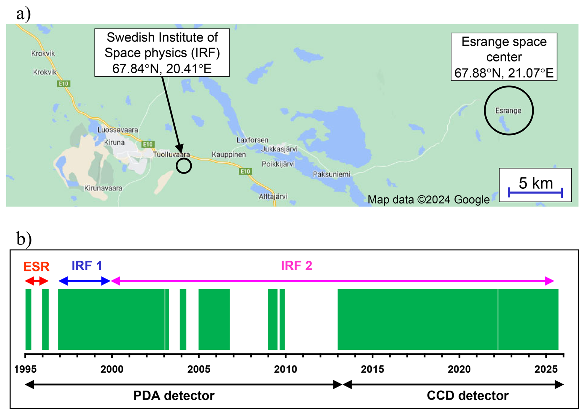
Figure 1 (a) Map with the two locations of the instrument (© Google maps); (b) timeline of the zenith DOAS measurements. ESR and IRF 1/2 indicate measurements at ESRANGE and the Swedish Institute of Space Physics near Kiruna, respectively. IRF 1 represents the period between December 1996 and October 1999 when the instrument was installed in a small hut on the roof of the institute; after October 1999 (IRF 2), the instrument was operated in a room inside the institute. Until 2013 a photodiode array detector (PDA), and since then a CCD detector was used.

3 Dependence of the high-resolution solar fit results on the fit settings

In this study, the KF is performed with the QDOAS software (Danckaert et al., 2017). For most applications, the overall wavelength range was set to 320–390 nm, and for all cases an ozone absorption cross section for 221 K (Burrows et al., 1999) was included in the fit. Optionally, also an intensity offset (Aliwell et al., 2002) or a Ring spectrum (calculated from the zenith-sky spectra, see Wagner et al., 2009a) were included. The number of spectral sub-windows was varied between 5 and 15, and the degree of the DOAS polynomial was varied between 3 and 5. Gaussian or super-Gaussian (Beirle et al., 2017) parameterisations were chosen to describe the ISRF. In this study we use the formulation of the super-Gaussian shape S(x) as function of the FWHM ω and the exponent k:

$$\begin{array}{}\text{(1)}& S\left(x\right)=A\cdot \exp \left[-\ln \mathrm{2}\cdot {\left(\mathrm{4}\cdot {\displaystyle \frac{{\left(x-x_{\mathrm{0}}\right)}^{\mathrm{2}}}{{\mathit{\omega }}^{\mathrm{2}}}}\right)}^k\right]\end{array}$$

with A the amplitude, x the wavelength, and x₀ the center wavelength. An alternative formulation as function of the variance σ² and the exponent k can be found in Beirle et al. (2017). We apply the KF to spectra measured around a solar zenith angle (SZA) of 90° (±0.5°), because such measurements are usually selected for the analysis of stratospheric trace gases (e.g. Götz et al., 1934; Noxon, 1975; Solomon et al., 1987; Aliwell et al., 2002). For measurements during twilight the light paths through the stratosphere can become very long (up to several hundred kilometers) making the measurements very sensitive for stratospheric absorbers. For smaller SZA, similar results of the KF are obtained, but the derived FWHM is usually (for clear days) smaller, because the strength of the Ring decreases with decreasing SZA (see also Sect. 3.3).

3.1 Sensitivity studies for selected spectra

Figure 2 shows results of KFs for two zenith-sky spectra, one measured with the old detector (left column) and the other with the new detector (right column). The first spectrum on 6 September 2002 was selected, because close to that day (3 September 2002) also Mercury line lamp measurements were made, to which the calibration results will be compared in Sect. 3.4 (between 3 and 5 September 2002 no zenith-sky measurements were made). The second spectrum on 6 September 2014 was chosen to have similar measurement conditions for both detectors. Figure 2a shows the FWHM as a function of wavelength obtained with a Gaussian parameterisation (as will be shown in Sect. 3.4, a Gaussian parameterisation fits the true ISRF of our measurements already quite well). The different symbols represent the results for different numbers of sub-windows. The black line is a 4th order polynomial fitted to the results using 10 sub-windows. The obtained FWHM for both spectra is around 0.6 nm and shows a weak wavelength dependence. The results for the different numbers of sub-windows vary by about ±0.01 nm. The variation is slightly larger for the old detector. In Fig. 2b results for a super-Gaussian parameterisation are shown. The FWHM is slightly larger (in particular at the ends of the spectral range) than for the Gaussian parameterisation. This is a reasonable result, because the second fit parameter (the exponent k) shows values somewhat larger than 2 (Fig. 2c), indicating that the ISRF has a slightly more box-like shape than a simple Gaussian parameterisation. Compared to the results for the Gaussian parameterisation, the fit results show slightly larger scatter. For wavelengths below about 330 nm often unrealistic fit results were found with FWHM up to larger than 1 nm (outside the range displayed in the figure) probably because of non-linearities caused by the increased ozone absorption.

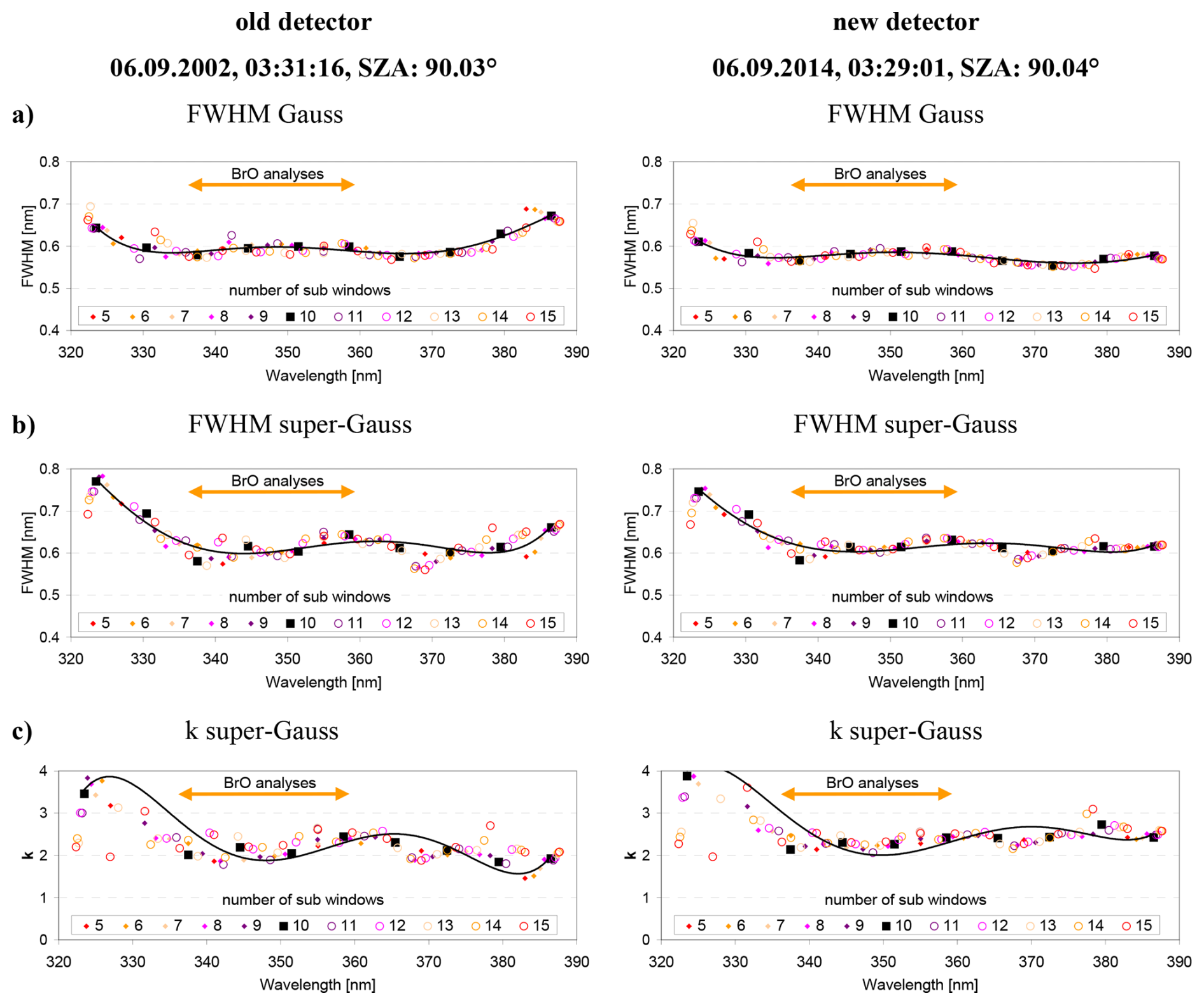
Figure 2 Results of the KF for two selected zenith-sky spectra taken at a SZA of about 90°, one from the old detector (left) and one for the new detector (right). The FWHM was either derived assuming a Gaussian (a) or super-Gaussian (b) parameterisation. From the fit with the super-Gaussian parameterisation also the second fit parameter k (see Beirle et al., 2017) was derived (c). The different symbols represent results for different numbers of fit windows. The black line is a polynomial of 4th order fitted to the results for 10 sub-windows. The horizontal arrow indicates the spectral range typically used for BrO analyses.

Also, the effect of additional fit parameters was tested. If a Ring spectrum or an intensity offset were also included in the KF, a larger variation of the FWHM was found for the old detector, while the results of the new detector were almost unchanged (Fig. A2). For the second fit parameter k of the super-Gaussian parameterisation, also larger variations for the old detector were found (values between 2 and 3). Finally, the effect of a third free fit parameter (describing the asymmetry) was tested for the super-Gaussian parameterisation. Almost unchanged results were obtained for the FWHM and the second fit parameter k, which is reasonable, since the line shape was found to be almost perfectly symmetric (the asymmetry parameter derived from the fit was close to zero). We also varied the order of the DOAS polynomial in the individual sub-windows (from 3 to 5) with a negligible effect on the KF results (not shown).

From these findings we conclude that (at least for this instrument) the most stable results are obtained for a Gaussian or super-Gaussian parameterisation without including a Ring spectrum or intensity offset. This finding is further explored and discussed in the following 2 sections. Using about 10 sub-windows (each covering 7 nm for the chosen total wavelength range) seems to be a good choice to obtain stable results and at the same time provide sufficient details about the wavelength dependency.

3.2 Results for the whole measurement time series

For a “perfect” instrument the ISRF would not change with wavelength and time. In this section these dependencies are tested for the whole period (1995 to 2025, with more than 1.1 million spectra) of the Kiruna measurements using daily measurements around SZA = 90°. Figure 3 presents time series of the FWHM obtained by KFs for 4 selected sub-windows (334–341, 341–348, 348–355, 355–362 nm), which cover the overall range of typical BrO fit windows (Aliwell et al., 2002; Hendrick et al., 2008, 2009; Rozanov et al., 2011; Parrella et al., 2013). The different panels show results for a Gaussian parameterisation with or without a Ring spectrum or intensity offset included (Fig. 3a–c) and for a super-Gaussian parameterisation (Fig. 3d). Several important findings are obtained:

1. Systematic seasonal variations are found, which could not be explained by variations of any instrumental or meteorological properties. It turned out that they are caused by the seasonal variation of the Ring effect between winter (with snow at the ground) and summer (without snow), for more details, see Sect. 3.3).

2. There is a rather large scatter of the results from day to day. This finding is caused by variations of the strength of the Ring effect due to the varying cloud cover (see e.g. Wagner et al., 2004, 2014), while noise of the measured spectra hardly contributes to this variation. A detailed discussion of the effect of clouds on the Ring effect is provided in Sect. 3.3.

3. The day-to-day variation is larger for the old detector than for the new detector. This may be caused to a small extent (see point 2) by the lower signal to noise ratio of the old detector. But the main reason is that frequent instrumental problems, e.g. re-starts of the instrument, change the instrumental properties, in particular the periodic structure of the instrumental light throughput caused by the Fabry–Pérot-etalon effect (see Sect. 4).

4. Only for the Gaussian parameterisation without including a Ring spectrum or an intensity offset (Fig. 3a), a consistent seasonal variation of the FWHM for the different spectral ranges is found. This finding indicates that if additional free fit parameters are allowed (Fig. 3b, c, d), varying parts of the initial change (here caused by the changing Ring effect) will be assigned to other free fit parameters. This interference is probably caused by the imperfect description (approximations) of the different effects (intensity offset, ISRF, and Ring correction) by their parameterisations in the KF.

5. The FWHM increases towards the end of the time series (since about beginning of 2023). This behavior is most clearly found for the Gaussian parameterisations without including a Ring spectrum nor an intensity offset, and is most probably caused by a real change of the ISRF. The reason for that change is unclear. Unfortunately, no atomic line lamp measurements during that period are available. In principle, it could also be indirectly caused by changes of other instrument properties like the straylight level (see point d). However, in a later analysis (Sect. 4.1) it is found that the intensity offset (or strength of the Ring effect) shows no systematic change during that period. Further results of the KF (spectral shift, intensity offset, strength of the Ring effect, and the exponent k of the super-Gaussian parametersation) are shown in Fig. A3 in the Appendix. The strength of the Ring effect is represented by the so-called Raman scattering probability (RSP, Fig. A3c), which describes the average probability of a measured photon to have undergone at least one Raman scattering event (Wagner et al., 2009a).

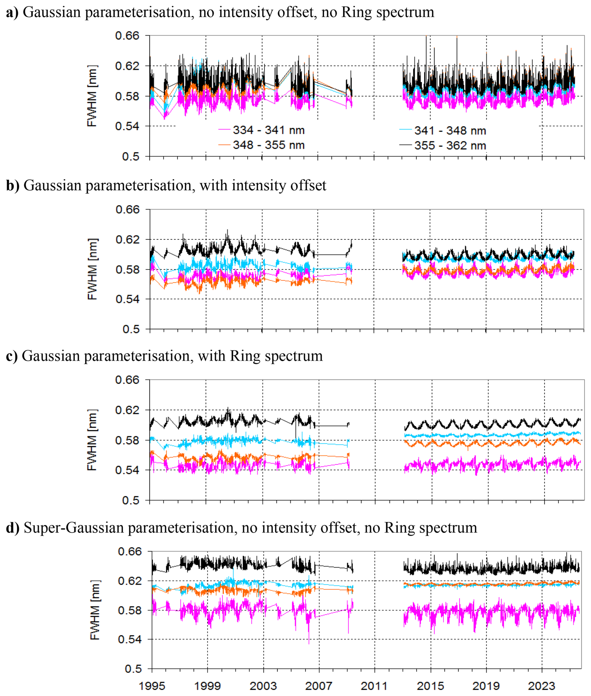
Figure 3 Time series of the FWHM determined for daily measurements (SZA between 89.5 and 90.5°) for the whole time series for 4 selected wavelength ranges. The different panels show results for different settings of the KF as described in the text.

Based on the above findings (1, 2, 3, 4) we recommend to use KFs with a rather simple ISRF parameterisation (preferably with only one free parameter). Also, no intensity offset nor Ring spectrum should be included. Only for such fit conditions, for our measurements consistent ISRF results as function of the wavelength and season are obtained. Here it is important to note that because of the broadening caused by the Ring effect the derived ISRF in general does not represent the true ISRF (as derived from atomic line lamp measurements). However, as will be shown in Sect. 3.4, at least for observations of stratospheric trace gases, the ISRF derived from the KF will be the better choice for the preparation of the reference spectra than the true ISRF.

Table 1 Reference spectra and further fit parameters used for the BrO analyses in this study (covering 2 to 4 BrO bands). The settings from Aliwell et al. (2002) are also shown. For the different fit ranges, different fit settings are used, mainly to account for the effects of the increasing ozone absorption towards shorter wavelengths. For the smallest fit range, a lower polynomial degree and only one Ring spectrum was used, because of the weak effect of the wavelength dependence of the atmospheric scattering processes.

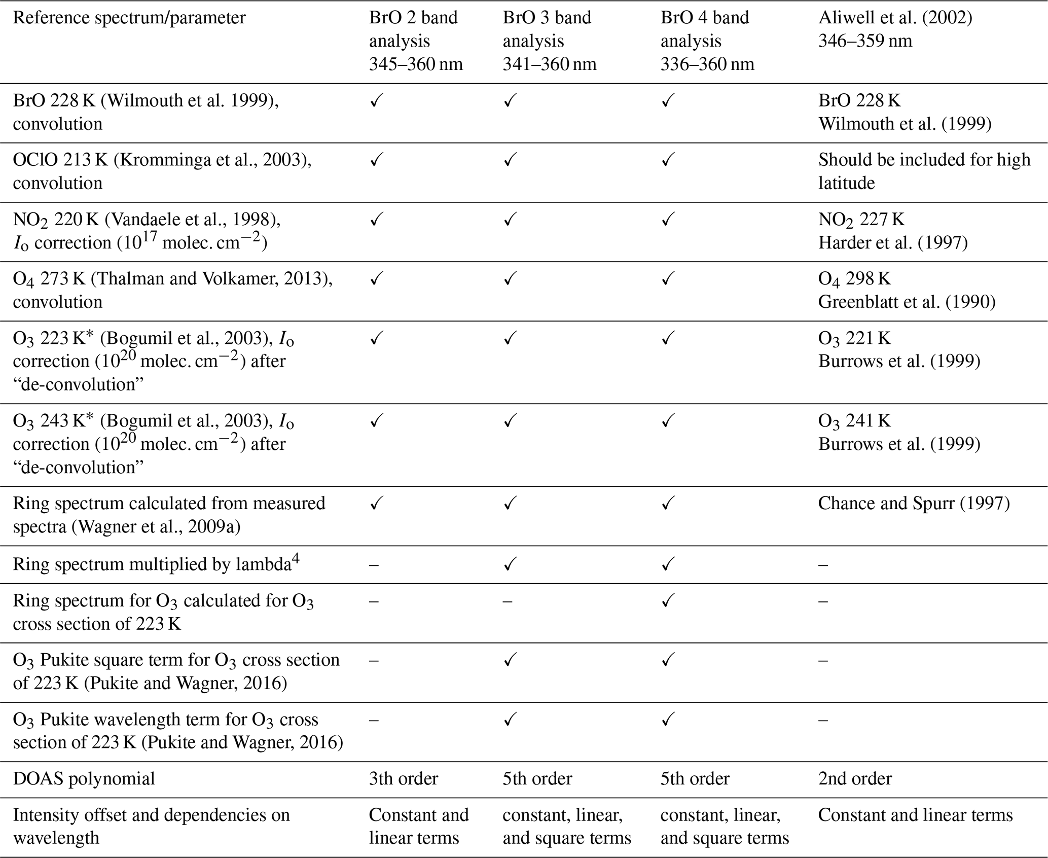
^∗ The original O₃ cross sections were de convolved before the I_o correction (as in Vandaele et al., 2005).

Finally, we performed DOAS analyses of BrO for the whole Kiruna measurement time series using trace gas reference spectra prepared based on the ISRF results from different KFs (Gaussian and super-Gaussian, see Fig. A7 in the Appendix). The KFs were performed for spectra from 17 February of the different years. On that day of the year, the SZA reaches 80° for the first time after the polar night (daily Fraunhofer reference spectrum, FRS, at 80° SZA are used for the BrO analysis). Further fit settings are provided in Table 1. For both analyses (using either Gaussian or super-Gaussian parameterisations) very similar results are found indicating that for our measurements the exact choice of the parameterisation is not critical. This might of course be different for other instruments and analyses and should be checked in individual cases.

3.3 Cause of the seasonal variation of the FWHM

The observed systematic seasonal variation of the FWHM (and also other parameters) derived from the KF was an unexpected finding. After various sensitivity studies it turned out that it is caused by the seasonal variation of the strength of the Ring effect, which depends (besides other factors) on the surface albedo. Because of its location in the far north, Kiruna is covered by snow during long periods in the winter. The seasonal variation of the snow depth at Kiruna for the years 2022 to 2025 is shown in Fig. 4a). Between about mid-May to mid of October, the snow depth is zero indicating a snow free surface. This seasonality is also represented by the measured zenith scattered light intensity (Fig. 4b), which depends strongly on the surface albedo because of the high backscattering probability of the Rayleigh scattering phase function.

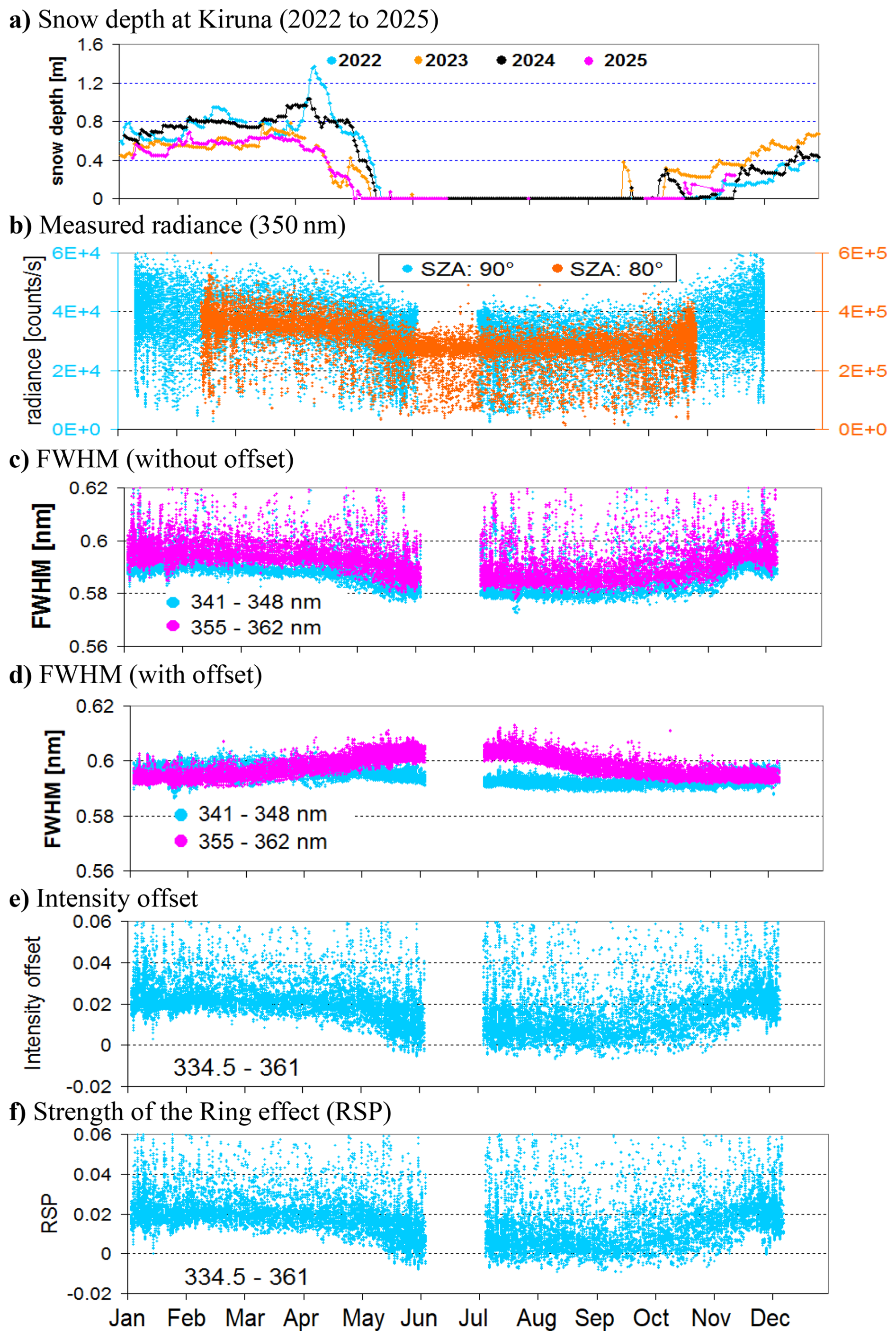
Figure 4 Seasonal variation (2014–2023) of (a) the snow depth (data obtained from the Swedish Meteorological and Hydrological Institute, https://www.smhi.se/data, last access: 17 November 2025). A snow depth of zero indicates a snow-free surface; (b) measured radiance (counts per second) for measurements with SZA between 79.5 and 80.5° (red) and 89.5 and 90.5° (blue); (c) FWHM derived from a KF without intensity offset; (d) FWHM derived from a KF with intensity offset; (e, f) intensity offset and RSP derived from an analysis with a pre-convolved high-resolution solar spectrum used as Fraunhofer reference spectrum (see Sect. 4).

The zenith scattered intensities show a systematic decrease during May and an increase during October to November. The different data points (blue and red) represent measurements for two different SZA ranges to cover the whole year including polar night and polar day. Figure 4c and d show the FWHM derived from the KF including or excluding an intensity offset (same data as in Fig. 3, but for clarity, only results for two wavelength ranges and for the new detector are shown). As discussed before, only for the fit results without allowing to fit an intensity offset, a consistent seasonal variation of the FWHM for the different wavelength ranges is found. Figure 4e and f show results from the modified fit procedure, which will be introduced in detail in Sect. 4. It uses pre-convolved (with the ISRF of the instrument) high-resolution solar spectra as FRS to avoid that part of the variation of the Ring effect is compensated by a variation of the ISRF. For that modified fit, larger wavelength intervals could be used, because the variation of the ISRF was already considered in the preparation of the FRS. From this fit, a consistent seasonal variation is also found for the derived intensity offset or the strength of the Ring effect. Correlation analyses of the quantities shown in Fig. 4b–f versus the snow depth (Fig. 4a) are presented in Fig. A4 in the Appendix. The variability caused by clouds dominates the variability of all quantities, but still for all quantities (except for the KF results including an intensity offset) a positive dependence versus the snow depth is found. These findings support the hypothesis that the observed seasonal variation of the FWHM derived from the “classical” Kurucz fit is caused by the variation of the Ring effect as a consequence of the changing surface albedo.

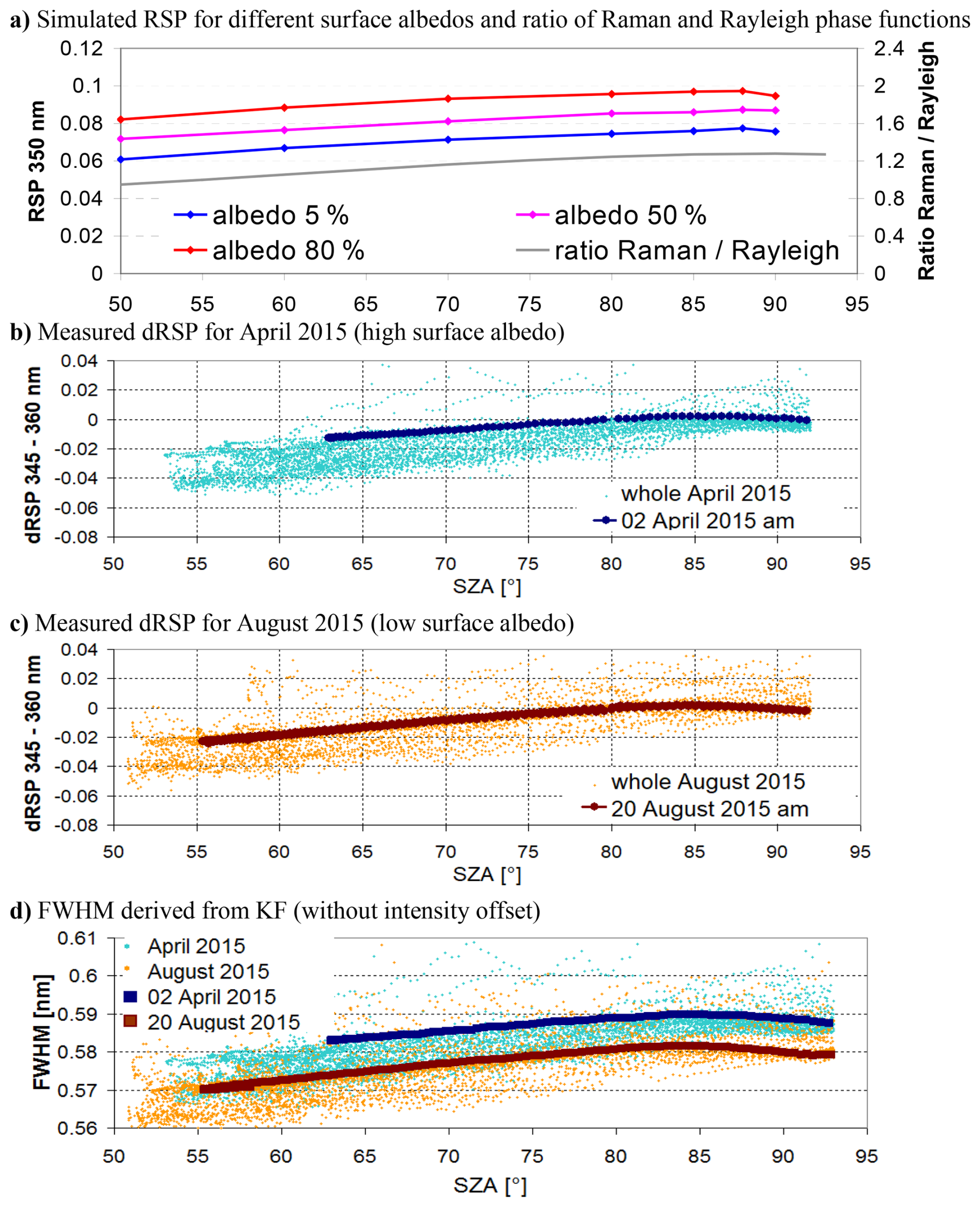
Figure 5 Dependence of different quantities on the SZA and surface albedo. (a) simulated RSP at 350 nm for different surface albedos and ratio of the Raman and Rayleigh scattering phase functions; for the radiative transfer simulations, the aerosol profile was assumed as box-profile from the surface to 1 km with an AOD of 0.2. The single scattering albedo and asymmetry parameter are set to 0.95 and 0.68, respectively. (b, c) Measured differential RSP (dRSP, relative to a FRS at 80° SZA) for April (high surface albedo) and August (low surface albedo) 2015. The big dots represent measurements on clear-sky days. (d) FWHM derived from KFs for the same measurements as in panels (b) and (c).

Further confidence for the Ring effect as cause for the variation of the FWHM arises from the investigation of its SZA dependence. In Fig. 5a radiative transfer simulations of the strength of the Ring effect (expressed as Raman scattering probability, RSP) for different surface albedos and as function of the SZA are shown. The RSP increases monotonously up to a maximum around 88° SZA. This increase is caused by the different phase functions for Rayleigh and Raman scattering as indicated by the similarity of the ratio of both phase functions (also shown in Fig. 5a) and the radiative transfer simulation results. It should be noted that for SZA above 90°, the radiative transfer simulations do not yield realistic results for the RSP because of the specific treatment (forcing) of the light paths between the sun and the first atmospheric scattering event (see Deutschmann et al., 2011). Figure 5b and c show the strength of the Ring effect (expressed as RSP) retrieved from measurements for two selected months, one with high surface albedo (April) and one with low surface albedo (August). For both months, also results for selected clear days are shown (filled markers). For the clear days, a similar monotonic increase of the RSP with increasing SZA until about 88° is found, in agreement with the simulation results (Fig. 5a). The RSP is analysed with respect to fixed Fraunhofer reference spectra at 80° SZA, one from 02 April 2015, and the other from 20 August 2015. Thus, no absolute RSP values are derived from the measurements, and similar (relative) RSP results are found for both months. It should also be noted that no fit of the intensity offset was allowed in the analysis in order to minimise the “cross-talk” between the fitted Ring spectrum and intensity offset. The results for the whole months (small dots) show a large variability caused by the influence of changing cloud cover (for the influence of clouds on the Ring effect, see e.g. Wagner et al., 2004, 2014), which also explains most of the scatter seen in Figs. 3 and 4. Figure 5d shows results of the FWHM derived from the KF without intensity offset for both months in 2015. A similar SZA dependence as for the other quantities is found, again confirming the Ring effect as cause for the change of the FWHM derived from the KF (without intensity offset).

The influence of clouds was further investigated as illustrated in Fig. A5 in the Appendix. In Fig. A5a the diurnal variation of the strength of the Ring effect and the O₄ dSCD for two selected days is shown. For the clear day, both quantities show a smooth and similar variation. In contrast, for the cloudy day both quantities show strong simultaneous short-term variations caused by light path changes (mainly affecting O₄) and changes of the number and type of atmospheric scattering events (mainly affecting the Ring effect). The different sensitivities to cloud effects also explain why the variation of the two quantities is not aways consistent. Figure A5b presents correlation analyses of both quantities for all measurements shown in Fig. 5. Also, results of radiative transfer simulations are shown. The comparison of the measurements and simulation results further confirms that the large variations of both quantities are caused by clouds, while the results for a clear day show only rather small variations. Figure A5c displays the correlation between the FWHM and the strength of the Ring effect for the measurements shown in Fig. 5. The strong correlation between both quantities confirms that the large variability of the FWHM derived for the KF is caused by the effects of clouds.

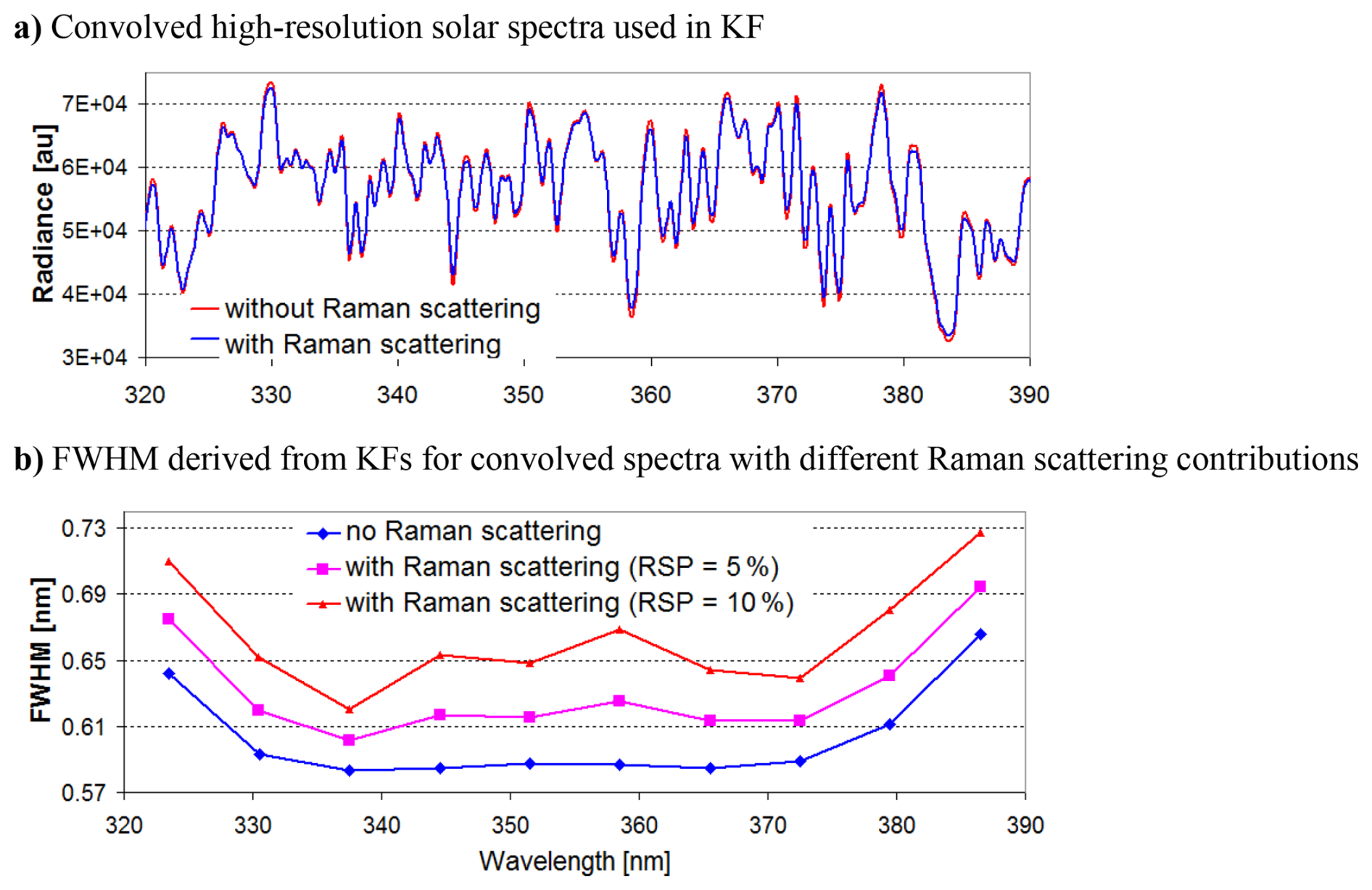
Figure 6 (a) Convolved high-resolution solar spectrum without and with the contribution of rotational Raman scattering (RSP of 10 %). (b) FWHM derived from KFs (without intensity offset) for spectra with different contributions of Raman scattering.

As a final test, the effect of adding different Raman scattering contributions to a simulated spectrum on the FWHM derived by a KF from that spectrum is investigated. For that purpose, a high-resolution solar spectrum is first convolved to the resolution of our instrument using the results of a KF to a measured spectrum. Then the contribution of Raman scattering is calculated for different strengths of the Ring effect and added to the convolved spectrum. Figure 6a shows the original convolved solar spectrum without the effect of Raman scattering (red) and with the contribution of Raman scattering (for a RSP of 10 %) added (blue). The optical depth of the Fraunhofer lines is clearly reduced in the blue spectrum (i.e. when including Raman scattering) compared to the red spectrum. In Fig. 6b the FWHM derived by a KF (without intensity offset) for spectra with different contributions of Raman scattering is shown. An increasing contribution of Raman scattering leads to an increasing FWHM. Since for zenith-sky measurements around SZA of 90°, the RSP (at 350 nm) is typically around 10 % (see Fig. 5a) the FWHM derived from the KF for such measurements is systematically broader than the true FWHM of the instrument (around 0.59 nm) by about 10 %. Even for lower SZA, the overestimation of the true FWHM will be quite substantial. As noted above, this is an important finding, because often the ISRF determined from a KF is used for the convolution of trace gas cross sections and the calculation of Ring spectra. Here it should be noted that the Ring spectra used in our DOAS analyses are not affected by the choice of the ISRF, because they are directly calculated from the measured spectra (Wagner et al., 2009a). The strength of the Ring effect increases with decreasing wavelength (see Fig. A6). Thus, its effect on the FWHM derived from the KF in the visible spectral range is smaller than for the examples discussed in this study.

Fortunately, for most stratospheric absorbers, the overestimation of the true FWHM caused by the Ring effect is not critical, since usually the last scattering event happens below the trace gas layer. Thus, the filling-in of stratospheric trace gas absorptions is similar to the filling-in of solar Fraunhofer lines (this hypothesis is further confirmed in Sect. 3.4). Nevertheless, for the analysis of trace gases located close to the surface, the overestimation of the FWHM might become a critical effect.

3.4 Comparison of the ISRF derived from the KFs to a measured line lamp spectrum

In the same way as the contribution of Raman scattering was added to a spectrum without Raman scattering contribution (Sect. 3.3, Fig. 6), it can also be subtracted from a measured spectrum. We perform such a correction for a measured spectrum on 6 September 2002, at 03:31 UTC (SZA = 90.028°). This spectrum was chosen, because 3 d before, Mercury line lamp measurements were performed, to which the ISRF derived from the KFs can be compared (no zenith-sky measurements closer in time to the Mercury line lamp measurements are available). The subtraction of the contribution of Raman scattering was performed assuming a RSP of 9 % (see Fig. 5a). Such a value is reasonable, because according to the measured radiance, colour index and O₄ absorption, no thick clouds were present during the acquisition of the spectrum. KFs were carried out in four ways: with Gaussian or super-Gaussian fit to the original spectrum (Fig. 7a), or with Gaussian or super-Gaussian fit to the original spectrum after removal of the Raman scattering contribution (Fig. 7b).

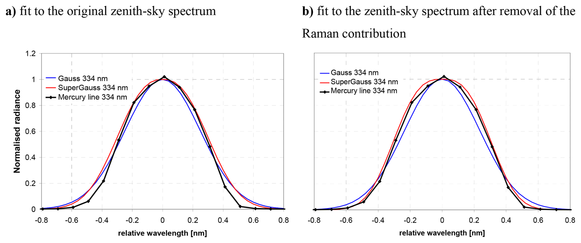
Figure 7 Measured slit function (black, Mercury line at 334 nm, measurement from 3 September 2002) and ISRF derived from KFs with Gaussian and super-Gaussian parameterisations to an original (a) and (b) Raman-corrected measured zenith-sky spectrum from 06 September 2002, 03:31 UTC (SZA: 90.028°). The Mercury lines in both plots are the same.

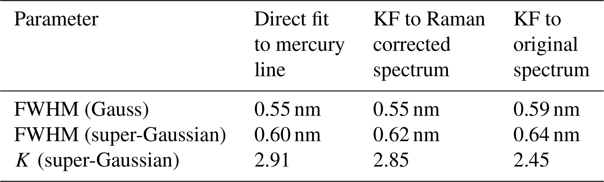
Best agreement with the measured ISRF is found for a KF to the Raman-corrected spectrum using a super-Gaussian parameterisation. Also, for the Gaussian parameterisation a slightly better agreement is found for the KF to the Raman-corrected spectrum than to the original spectrum, but the improvement is smaller. Here it should be noted that the better agreement to the measured ISRF does not necessarily mean that the ISRF derived from the Raman-corrected spectrum is a better choice for the preparation of the reference spectra for the analysis of stratospheric absorbers (see below). The results from the KFs and direct fits to the measured Mercury spectrum are summarised in Table 2 confirming the better agreement of the measured ISRF with the ISRF derived from the KF for the Raman corrected spectrum. In spite of this good agreement, it should be noted that the detailed procedure of the Mercury line lamp measurement on 3 September 2002 was not well documented. In particular, it is not clear how exactly the lamp light was fed into the telescope of the instrument. Therefore, such comparisons should be repeated in future studies with well controlled and documented measurement conditions.

Table 2 Gaussian and super-Gaussian parameters derived from KFs to zenith-sky spectra and from direct fits to a Mercury lamp spectrum (for more details see text).

In a next step, the four ISRF derived from the KFs to the spectrum from 6 September 2002, (1 – with Gaussian fit to the original spectrum; 2 – with super-Gaussian fit to the original spectrum; 3 – with Gaussian fit to the Raman corrected spectrum; 4 – with a super-Gaussian fit to the Raman corrected spectrum) were used to prepare 4 sets of trace gas reference spectra, which then were used for the BrO analyses in 3 spectral ranges for the year 2002 (Fig. A8). These sets of reference spectra were used for the analysis of the whole year. For the analyses using the ISRF from the original spectrum, reasonable and consistent BrO results are obtained. In contrast, for the analyses using the ISRF from the Raman-corrected spectrum, inconsistent results are found. Moreover, during summer, the BrO dSCDs are found to be very low, not in agreement with model results (e.g. Sinnhuber et al., 2002). This confirms the expectation from the end of Sect. 3 that the ISRF derived from the KF to the original spectrum is the best choice for the analysis of stratospheric absorbers, because the stratospheric trace gas absorptions are affected in a similar way by the Raman scattering as the solar Fraunhofer lines.

Finally, the question arises, which ISRF should be used for long-term trace gas analyses if the Ring effect changes with season (or also on a shorter time scale with changing cloud cover). For the measurements in Kiruna, the FWHM of an ISRF derived for measurements above terrain with high surface albedo will be too broad for measurements in summer, while the FWHM of an ISRF derived for measurements above low surface albedo will be too narrow for measurements in winter. To assess the resulting errors for the Kiruna measurements, we performed two BrO analyses using either a fixed ISRF (derived from a measured spectrum in February) for the whole year or varying ISRFs determined for individual 2-weeks periods. The comparison results are shown in Fig. A9. While overall, the results of both analyses are very similar, also systematic deviations (up to about 1 × 10¹³ molec. cm⁻²) occur in summer, when the ISRFs derived from measurements over snow do not fit the spectra measured over low surface albedo. Thus, we conclude that the analysis using a varying ISRF gives the more accurate results. Nevertheless, the differences are small, and also the analysis using a fixed ISRF could be sufficient for trend studies.

4 Analysis with pre-convolved high-resolution solar spectra

Because of the limitations of the KF in determining reasonable results for the intensity offset (or in general: possible biases caused by additive intensity components, e.g. spectrograph straylight), an alternative method is proposed in this Sect.. The basic idea is to perform a classical DOAS analysis, but to replace the measured FRS by a convolved (by the ISRF of the measured spectra) high-resolution solar spectrum. Such a method was already used by Lübcke et al. (2016) for the analysis of SO₂ in volcanic plumes. In that study the focus was on retrieving reliable SO₂ results without possible biases from contaminated FRS (having seen part of the SO₂ plume). They found that for the strong SO₂ absorption, this method worked quite well, and they also derived spectral structures caused by instrumental effects from these analyses by principal component analysis. Including these spectral structures in the SO₂ DOAS analysis as additional reference spectra largely improved the fit results.

In this section, we apply a similar, but more straight-forward method. We directly investigate the residual structures from a DOAS fit with a pre-convolved high-resolution solar spectrum as FRS. Our main aim is not the improvement of a DOAS fit, but we are interested in the low frequency structures of the fit residuals themselves, which are extracted from the DOAS polynomials p(λ) of the spectral analysis:

$$\begin{array}{}\text{(2)}& \begin{array}{rl}\ln \left(I_{\mathrm{measured}}\right):=& \ln (I_{\mathrm{solar},\mathrm{conv}}+I_{\mathrm{offset}})\\ & +\sum S_i\cdot {\mathit{\sigma }}_i+p\left(\mathit{\lambda }\right)+\mathrm{residual}.\end{array}\end{array}$$

Here I_measured, and I_solar,conv are the normalised (dimensionless) measured and convolved solar spectra, respectively. S_i and σ_i are the considered trace gas absorption cross sections and corresponding SCDs. I_offset is an intensity offset fitted to the convolved solar spectrum. In order to keep the fit simple, only the two most important trace gases (O₃ and NO₂) were included in the fit, and a constant intensity offset was chosen.

The ISRF and spectral calibration for the convolution of the solar spectrum are taken from a KF (without intensity offset) to the first measurement of a given year reaching a SZA of 80° after the polar night, which occurs at Kiruna around 17 February. The convolved high-resolution solar spectrum is then used as FRS for the analysis of all measured spectra of the chosen year.

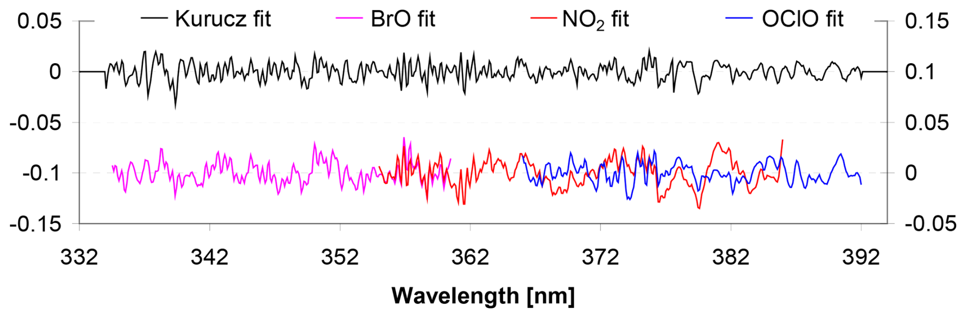
Figure 8 Residual structure for a KF without intensity offset (black, left y-axis) and the DOAS analysis with a convolved solar spectrum (coloured lines, right y-axis) of a measured spectrum from 6 September 2002, 03:31 UTC (the same spectrum as used in Fig. 7). The magenta line is the residual for the wavelength range 334.5–360.5 nm (labeled BrO fit), the red line for 355–386 nm (labeled NO₂ fit), and the blue line for 366–392 nm (labeled OClO fit) corresponding to typical fit windows for these trace gases.

Figure 8 shows a comparison of the residuals of the analysis of a measured spectrum with the convolved solar spectrum and a residual of the same spectrum using a classical KF. Overall, very similar residual structures are found with slightly higher values for the analysis with the convolved solar spectrum. This finding is not unexpected, because for the KF 10 sub-windows (with widths of 7 nm) were used, while for the analysis with the convolved solar spectrum three larger fit windows with widths between 26 and 31 nm were used. The three spectral ranges for the analysis with the convolved solar spectrum were chosen to cover typical fit windows for the analysis of BrO, NO₂, and OClO. In principle, also larger spectral ranges could have been chosen for the analysis with the convolved solar spectrum, but because of the very strong Fabry–Pérot etalon effect of the old detector (see below) and the limitation of the maximum degree (8) of the DOAS polynomial in the QDOAS software, no stable convergence was found for larger fit windows. The procedure described above will be used in the following sub-sections to quantify the (relative) intensity offset, Ring effect, and light throughput (and in particular their temporal variations) of the Kiruna measurements.

4.1 Time series of intensity offset and strength of the Ring effect

The results of the fitted intensity offset and strength of the Ring effect (RSP) derived from the analysis of daily measurements around 90° SZA with convolved solar spectra are shown in Fig. 9. For both quantities very similar results are found. Moreover, the values for the different spectral ranges show a consistent temporal evolution, and for the new detector also very similar absolute values. The systematic seasonal variation reflects the effect of the changing snow cover (see Sect. 3.3). For the old detector, larger values are found probably indicating larger contributions from spectrograph straylight or insufficient offset and dark current correction.

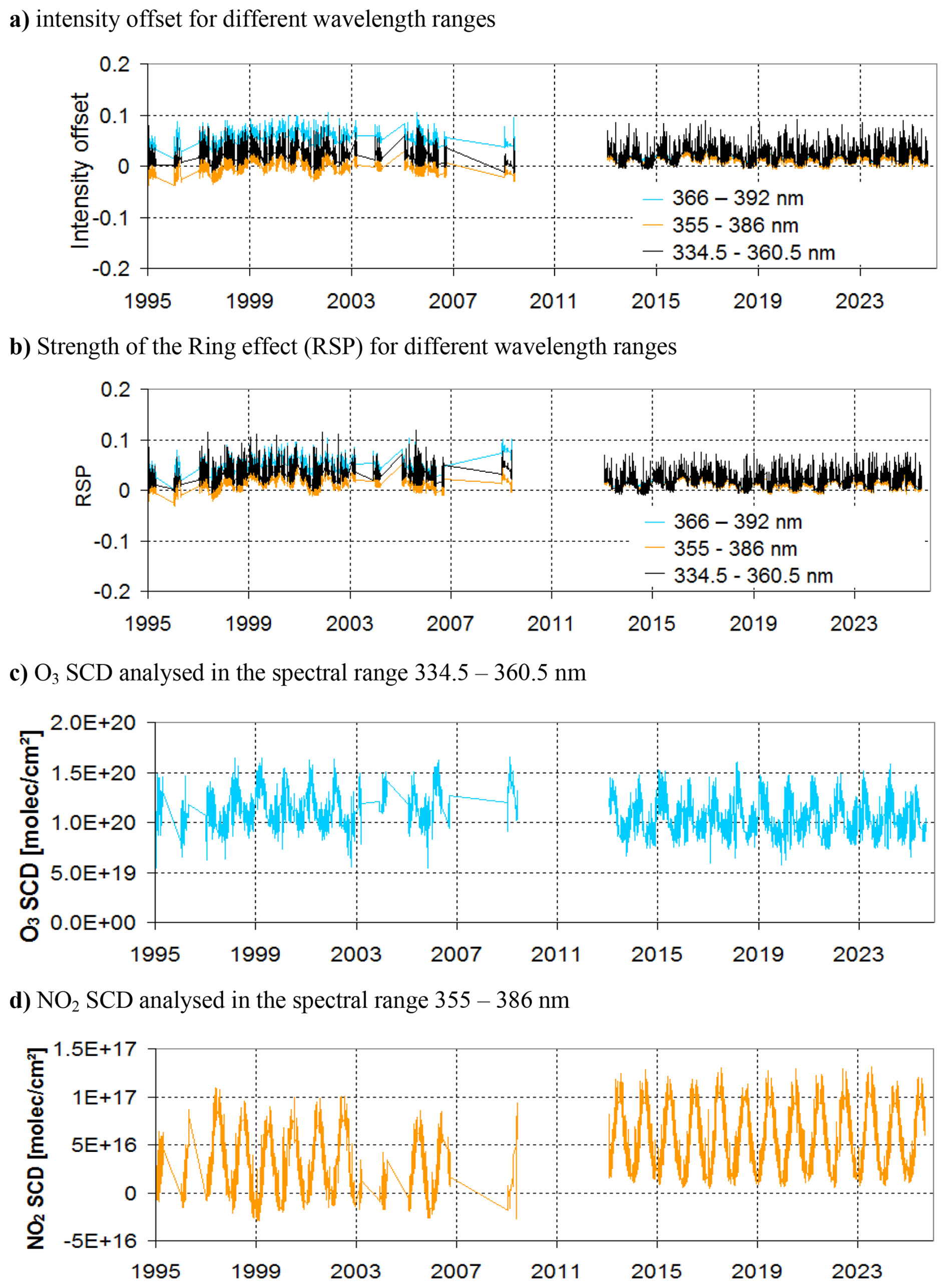
Figure 9 Retrieved intensity offset, RSP and the SCDs of O₃ and NO₂ from the DOAS analysis with convolved sun spectra. Results for daily measurements (SZA = 90 ± 0.5°) and for three different spectral ranges.

For the new detector, the values of the fitted intensity offset and the RSP are typically below 3 %. Here it should be noted that also the high-resolution solar spectrum might be affected by a non-zero intensity offset. Thus, the obtained values represent the differences between the measured spectra and the convolved solar spectrum (measured spectrum minus solar spectrum). Nevertheless, from these differential results it can still be derived how the intensity offset of the instrument changes with time. The results in Fig. 9 show that especially for the new detector, no substantial long-term changes occur. In particular, no changes are found towards the end of the time series. This indicates that the increase of the FWHM found after beginning of 2023 (Fig. 3) is not caused by an increasing intensity offset. It rather represents a real change of the ISRF. The reason for this change is not clear, but might be caused by changes of the whole instrumental setup due to material fatigue.

In Fig. 9 also the results for the dSCDs of O₃ and NO₂ are shown. Both results show reasonable seasonal variations, but for NO₂ also artefacts (e.g. negative values for the old detector and the jump between the results of both detectors) are seen. These results indicate that also trace gases (with large atmospheric optical depths) can be analysed using a convolved solar spectrum as FRS (as also found by Lübcke et al., 2016). However, the accuracy of the results is worse compared to analyses with FRS measured by the same instrument.

4.2 Determination of the light throughput of the instrument

The light throughput describes the amount of light that passes through an optical system. It is determined by the instrument's étendue (product of aperture angle and entrance area, e.g. Platt et al., 2021), but also by the spectral characteristics of the optical elements inside the instrument. In DOAS instruments, most important contributions come from the quantum efficiency of the detector, the efficiency of the grating, and the transmission of optical filters used to suppress instrument straylight. Additional contributions can arise from the Fabry–Pérot etalon effect (Pérot and Fabry, 1899), an interference effect between reflecting surfaces on top of the detector (see also Stutz and Platt, 1997). Since on the surface of a cooled detector thin ice layers can build up, the Fabry–Pérot etalon effect can also vary with time. Especially after a restart of an instrument (in particular after a restart of the detector cooling), discontinuities of the Fabry–Pérot etalon effect occur. The Fabry–Pérot etalon effect can be visualised and quantified from measurements with a halogen lamp, which provides a smooth spectrum. Such measurements are shown in Fig. 10, one for the old and another for the new detector. For the old detector, periodic structures with widths of about 10 nm are clearly visible. For the new detector no such Fabry–Pérot etalon structures are seen because of different properties of its detector coating. For both detectors a strong reduction of the intensity for wavelengths above 380 nm is found caused by an optical filter (UG-5) used to suppress the contribution to spectrograph straylight from longer wavelengths. Because of the relatively narrow spectral width and strong amplitude (about ±15 %), the Fabry–Pérot etalon effect of the old detector can have an impact on the trace gas results, especially if large temporal differences between the measured spectra and the FRS exist. Fortunately, for analyses using daily FRS, the Fabry–Pérot etalon effect is usually no problem, because the spectral structures in both the measured spectra and the daily FRS are almost identical.

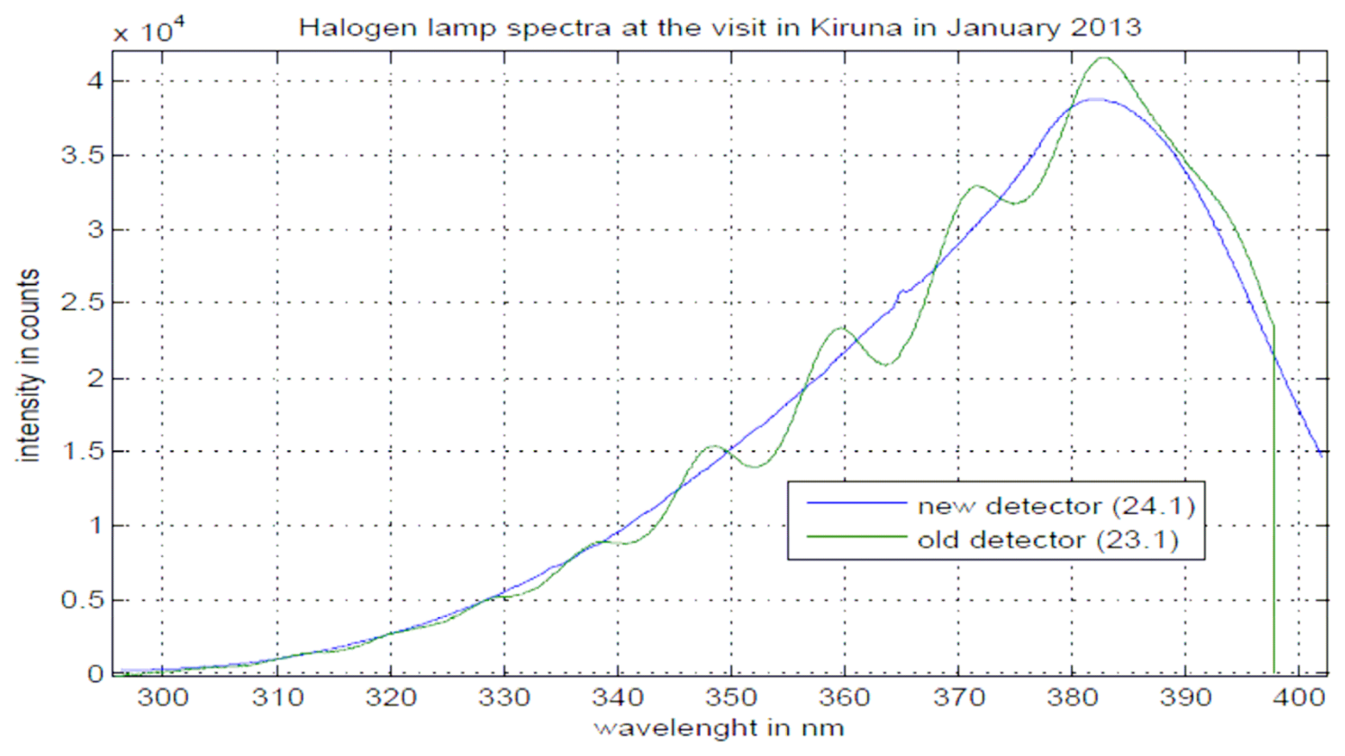
Figure 10 Halogen lamp spectrum of the old (green, 23 January 2013) and new detector (blue, 24 January 2013). Image from Gu (2019).

From the DOAS polynomial (see Eq. 2) of an analysis with a convolved solar spectrum the wavelength-dependent light throughput of a DOAS instrument can be determined. Here it should be noted that usually the DOAS instruments are not radiometrically calibrated. Thus, not the absolute light throughput can be determined from the DOAS fit using a convolved solar spectrum as FRS, but the fit results represent the light throughput relative to that of the high-resolution solar spectrum. Nevertheless, the most relevant property for DOAS analyses is the spectral variation of the (relative) light throughput of the instrument. In our analysis and interpretation it is assumed that the solar spectrum itself does not show significant wavelength-dependent modulations. As will be shown below, this assumption is well fulfilled for the spectral range considered here. Another important assumption is that the wavelength-dependence caused by atmospheric scattering is negligible. In Appendix A3 it is shown that for the selected zenith-sky spectra the wavelength-dependence is indeed small causing a reduction of the radiance at 330 nm of about 13 % compared to 390 nm.

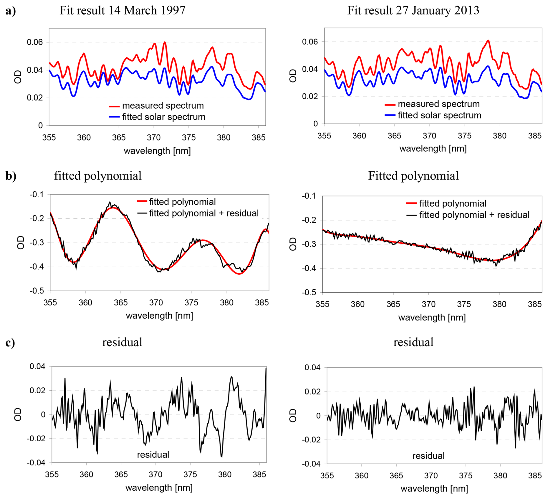
Figure 11 Fit results for selected spectra of the old (14 March 1997, 05:10 UTC, SZA: 90.2°) and new (27 January 2013, 13:15 UTC, SZA: 90.13°) detector using a convolved high-resolution sun spectrum as FRS. Results for the other spectral ranges (334.5–360.5 and 366–392 nm) are shown in Fig. A11 in the Appendix.

In Fig. 11 results of the analyses of spectra from both detectors using convolved high-resolution solar spectra as FRS are shown. In the top panel the fit results are shown. Already there, for the old detector the effect of the Fabry–Pérot etalon structure is clearly visible: the differences between the measured spectrum and the convolved solar spectrum vary strongly with wavelength. For example, small differences between both spectra are found around 355, 363 and 374 nm, while for wavelengths around 368 and 380 nm the differences are large. Such periodic variations are not seen for the new detector (right). The spectral variations caused by the Fabry–Pérot etalon effect are also clearly represented by the fitted DOAS polynomial (Fig. 11b left), while for the new detector the DOAS polynomial shows a smooth variation. Only above 380 nm the effect of the UG-5 filter becomes obvious in the DOAS polynomials obtained for both detectors. Similar results for the other chosen spectral ranges (334.5–360.5 and 366–392 nm) are shown in Fig. A11.

Next, the light throughputs derived from the DOAS polynomials (Fig. 11b) are compared to those derived from the halogen lamp measurements. Before the comparison is performed the following preparation steps are applied:

From the DOAS polynomial p(λ), the (relative) light throughput T_DOAS is calculated by inverting the Beer-Lambert law:

$$\begin{array}{}\text{(3)}& T_{\mathrm{DOAS}}=\exp \left(-p\left(\mathit{\lambda }\right)\right).\end{array}$$

From the lamp measurements the light throughput T_lamp is calculated by dividing the lamp measurement S_lamp by the emission spectrum (Planck function) of a black body of the temperature of the halogen lamp:

$$\begin{array}{}\text{(4)}& T_{\mathrm{lamp}}={\displaystyle \frac{S_{\mathrm{lamp}}}{B\left(T\right)}}.\end{array}$$

Best agreement between the lamp spectra and the black body emission spectra was found for temperatures of around 3100 and 2800 K for the selected lamp spectra of the old and new detector, respectively.

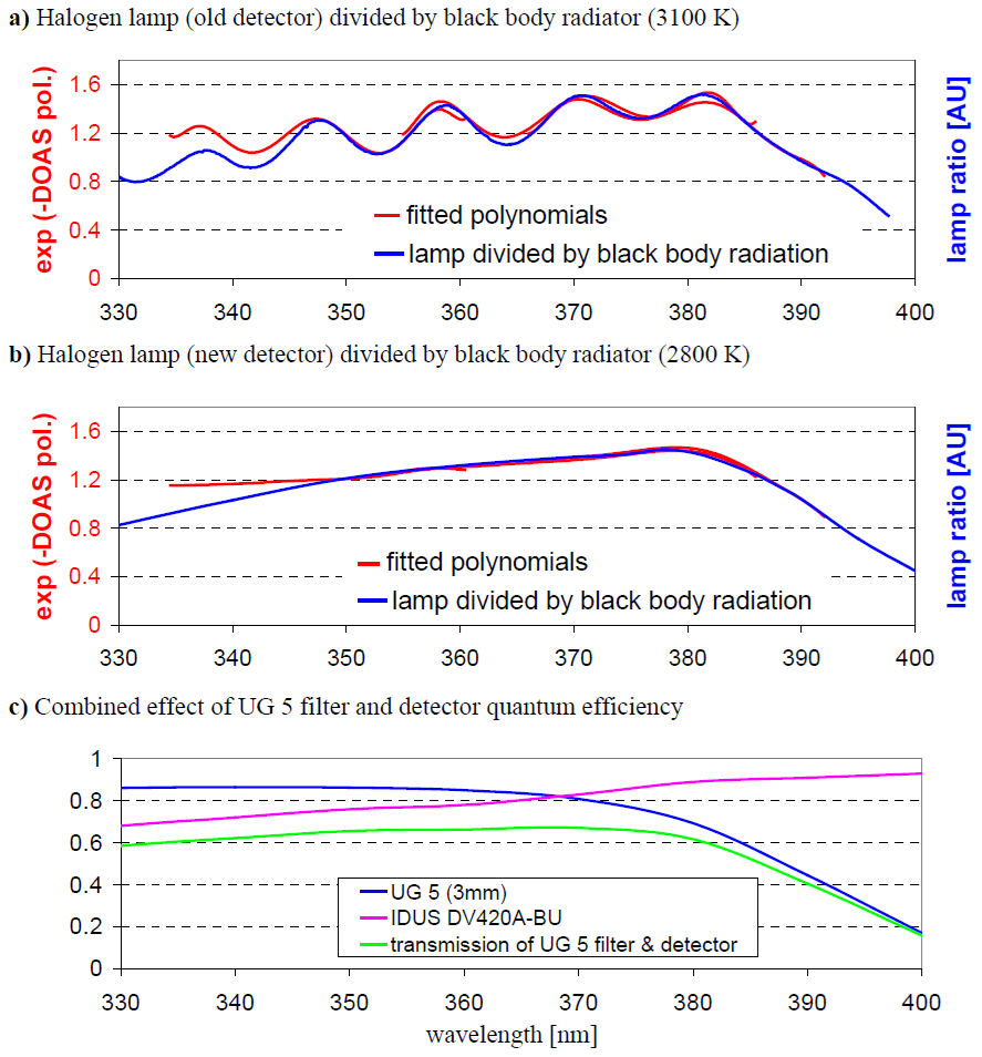
Figure 12 Comparison of the optical throughputs for measurements with the old detector (a) and new detector (b) derived from the fitted DOAS polynomials and lamp measurements (Eqs. 3 and 4). In panel (c) the combined transmission for the new detector (IDUS DV420A-BU) calculated from its quantum efficiency and the transmission of the UG-5 filter is shown.

The comparison of the light throughputs for the old and new detector derived from Eqs. (3) and (4) is shown in Fig. 12a, b. Different y-axes are used for the results from the lamp measurements and DOAS fits, because of the different absolute values. Here it should also be noted that the measured spectra and convolved solar spectra are normalised before the fit procedure, which explains the values derived from the DOAS polynomial close to unity.

Concerning the spectral variation of the light throughput, for both detectors good qualitative agreement is found. For the old detector, the Fabry–Pérot etalon effect is clearly visible in both curves, while for the new detector a flat wavelength dependence is found. For both detectors, also the influence of the UG-5 filter for wavelengths above 380 nm is seen. Interestingly, for both detectors, also the light throughput below about 350 nm derived from the DOAS polynomials is higher than from the lamp measurements. One probable explanation is a reduced transmission of the glass of the lamp bulb for such short wavelengths. Also, the missing knowledge of the exact lamp temperature and the effects of atmospheric scattering might contribute to the differences between both results. The overall good agreement between the results of the DOAS polynomials and the lamp measurements confirms that the high-resolution solar spectrum is not affected by strong wavelength-dependent modulations. In Fig. 12c the combined light throughput of the detector quantum efficiency and the UG-5 filter is shown (green line). The general spectral shape agrees roughly to that in Fig. 12b, but there are also differences, in particular for wavelengths above 380 nm. The reason for these differences is not completely clear, but might be related to the wavelength dependence of the efficiency of the grating. Unfortunately, no information about the wavelength-dependent efficiency of the grating could be found.

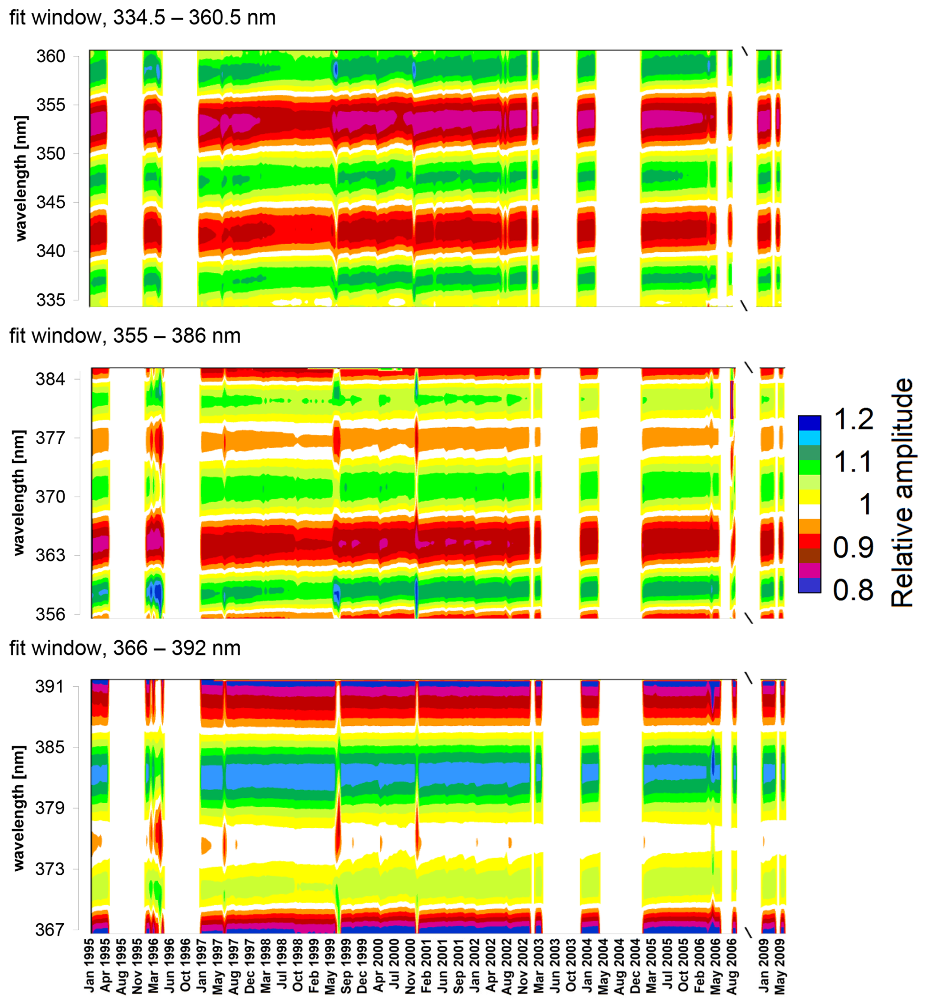
Figure 13 Time series of the wavelength-dependent Fabry–Pérot etalon structures for the three selected fit windows. Shown are the high-pass filtered (division by a linear fit) throughputs calculated from the DOAS polynomials according to Eq. (3) for every 1st and 15th day of a month from 1995 to 2009.

Figure 13 shows time series of the Fabry–Pérot etalon structures for the whole time period of the old detector (1995–2009) for the 3 selected fit ranges. The overall structure of the Fabry–Pérot etalon structures stays similar over the whole time period, but short and long-term variations, mainly after restarts of the instrument, are clearly visible.

4.3 Correction of the Fabry–Pérot etalon effect

The Fabry–Pérot etalon effect of the old detector causes amplitude variations of the measured spectra up to about ±15 % (see Figs. 11, 12, 13, and A11). With the knowledge of the wavelength-dependent light throughput (e.g. derived from the DOAS polynomial), this strong wavelength dependence can be corrected. We applied such a correction on a daily basis by dividing the measured spectra by the light throughputs obtained from the DOAS fits according to Eq. (3). In that way we created a second set of “corrected” spectra, to which we applied the BrO analyses in the same way as to the original spectra.

The results of both analyses are compared in Fig. 14. While for the new detector, almost identical results are found, strong and systematic differences appear for the old detector, related to the strong Fabry–Pérot etalon effect. The differences of the retrieved BrO dSCDs reach up to about 40 % for the fit windows 341–360 and 335–360 nm, and even up to about 60 % for the fit window 336–360 nm with different signs for the different fit windows. For the corrected spectra, better consistency between the 3 fit windows than for the original spectra is found indicating that the etalon correction leads to improved results.

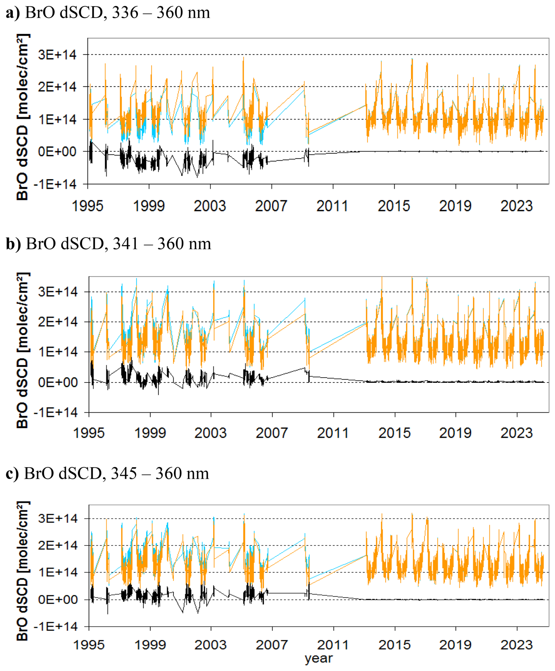
Figure 14 Comparison of the BrO results from DOAS analyses of the original (light blue) and corrected (orange) spectra. The black lines represent the difference between both results (original minus corrected).

At first glance, the differences between the BrO results for the original and corrected spectra seem surprising. Since the correction of the Fabry–Pérot etalon effect was consistently applied for the measured spectra including the daily FRS (measured zenith-sky spectra at 80° SZA), it was expected that the results for the original and corrected spectra should be identical (because the modulations of the Fabry–Pérot etalon effect cancel out in the DOAS analysis). But as shown in Fig. 14, strong and systematic differences were found. It turned out that these differences only occur if the BrO analysis was performed with a non-linear fit (the non-linearity is caused by the allowed spectral shift and fitted intensity offset). If, however, the fit was as a test reduced to a purely linear fit (with no shift and intensity offset allowed), identical results were obtained for the original and corrected spectra. The effect of excluding the free spectral shift or intensity offset in the DOAS analysis was further investigated. For that purpose, different DOAS analyses of the original spectra (no etalon correction applied) were performed for two weeks in May 1998. BrO dSCDs were retrieved with either no intensity offset allowed, no shift allowed, or no intensity offset and no shift allowed. The corresponding deviations from the results of the standard analyses (with shift and intensity offset allowed) are plotted versus the shift or intensity offset obtained from the standard analysis. The corresponding results are shown in Fig. A10. Systematically different results are found for the different fit windows indicating that each fit window is affected in a specific way by the respective part of the etalon modulation. The smallest deviations are found for the largest fit window, which contains most spectral information. Except for the smallest fit range, the largest differences from the standard analyses are found if no spectral shift is allowed, and these differences are correlated with the spectral shift. Similarly, if no intensity offset is allowed, the differences are correlated with the intensity offset. The systematic dependence on the spectral shift is similar to the so-called tilt effect (e.g. Rozanov et al., 2011; Lampel et al., 2017, and references therein), but the influence of the Fabry–Pérot etalon effect on the DOAS analyses is more complex. In contrast to the monotonic tilt effect, it causes periodic structures affecting different parts of the fit windows in opposite ways.

For stronger atmospheric absorbers, the differences of the results of the original and corrected spectra are much smaller: for ozone, they were found to be below 1 % for the fit window 345–360 nm, and below 3 % for the other two fit windows. For NO₂ they are below 3 % for all three fit windows (except for the winter months when the NO₂ dSCDs are close to zero). The findings from the results shown in Fig. 14 might be important also for measurements with other instruments with variable and wavelength-dependent light throughputs. Instrument operators should thus characterise the light throughputs of their instruments, e.g. by the method introduced in this study.

5 Summary and conclusions

The characterisation of spectroscopic properties of DOAS instruments is important for accurate trace gas retrievals. Especially for the analysis of trace gas trends from long-term measurements, the continuous monitoring of instrumental properties is crucial to ensure that the retrieved trends represent true atmospheric variations and are not caused by instrumental artefacts. In this study, we tested, refined, and extended an existing method (the so-called Kurucz fit, KF) for the characterisation of instrumental properties (e.g. the ISRF, intensity bias, or light throughput) using high-resolution solar spectra. We applied different variants of this fit to long-term zenith-sky DOAS measurements (1995–present) at Kiruna (northern Sweden). The main findings of our study are:

• a.

  The exact number of sub-windows and the choice of the degree of the DOAS polynomial of a KF are not critical. We recommend a spectral width of the sub-windows of about 5 to 10 nm. The accuracy of the FWHM derived for such settings is about ±0.01 nm.

• b.

  We tested Gaussian and super-Gaussian parameterisations of the ISRF. For the Kiruna measurements the exponent k of the super-Gaussian parameterisation was found to be between 2 and 2.3 indicating only small deviations from a pure Gaussian shape. Also, very similar BrO results were obtained using either a Gaussian or super-Gaussian parameterisation. For other instruments, the deviations from a Gaussian shape might be larger and a super-Gaussian parameterisation (or a measured ISRF) might be better choices.

• c.

  We found inconsistent results of the FWHM (different values and different temporal variations in neighboring spectral ranges) if an intensity offset or a Ring spectrum was included in the KF. For such fit settings there are probably too many free fit parameters which are sensitive to additive intensity contributions. For KFs without intensity offset nor a Ring spectrum included, consistent FWHM results were obtained. Therefore, in general such simple fit settings are recommended for the determination of realistic ISRF. If possible, also simple ISRF parameterisations (e.g. Gaussian parameterisations or measured slit functions, which are allowed to be squeezed during the KF) are recommended. These conclusions are derived for our zenith-sky DOAS measurements in the UV spectral range. Further studies should be carried out for different instruments and wavelength ranges. Possibly, for instruments with higher spectral resolution, the effects of rotational Raman scattering and the width of the ISRF could be better separated.

• d.

  We found that the Ring effect leads to a systematic broadening of the derived ISRF compared to the true ISRF (derived from measurements using atomic line lamps) by +10 % (for a typical UV zenith-sky spectrum at 90° SZA). The broadening of the FWHM can be weaker or stronger depending on the observational geometry, wavelength, surface albedo and cloud cover. The broadening effect of Raman scattering was also confirmed by the direct comparison of the ISRF derived from KFs to those derived from line lamp measurements. The dependence of the derived ISRF on the strength of the Ring effect is a fundamental effect and leads to the question, which ISRF is the correct one for the preparation of trace gas reference spectra. Here different choices should probably be made for different measurement geometries and trace gas locations: For zenith-sky measurements like those in Kiruna, the focus is typically on stratospheric trace gases, for which the first atmospheric scattering event is typically below the trace gas layer and thus the filling-in caused by the Ring effect is similar for the solar Fraunhofer lines and the trace gas absorptions. Hence, the ISRF derived from a KF of a measured spectrum (affected by the Ring effect) will be a good choice for the convolution of the trace gas reference spectra. Nevertheless, care should be taken that the spectra selected for the KF are not influenced by the presence of optically thick clouds, which can lead to a strong increase of the Ring effect caused by multiple scattering. In contrast, for measurements of trace gases located close to the surface, in particular for MAX-DOAS observations and satellite observations in nadir geometry, a spectrum without a contribution from Raman scattering, e.g. a direct sun spectrum (or an earth shine spectrum after the subtraction of the Raman scattering contribution), might be a better choice.

• e.

  Measurements at lower latitudes (without the presence of snow in winter) will be less affected by the seasonal changes of the Ring effect, but for measurements during twilight, the RSP at 90° SZA is still rather high (for a surface albedo of 0.05 it is about 0.075 for 350 nm and about 0.05 for 440 nm). Fortunately, for albedo values below about 0.1 the dependence of the RSP on surface albedo becomes almost negligible (changes are below about 0.002 at 320 nm, and below about 0.001 for wavelengths > 400 nm, see Fig. A6). For MAX-DOAS measurements, the situation is more complex than for zenith-sky observations, because the Ring effect depends not only on SZA, but also on the elevation and relative azimuth angles as well as on the aerosol load (Wagner et al., 2009b). However, since MAX-DOAS measurements are usually analysed for smaller SZA ranges than zenith-sky observations, in general the strength of the Ring effect is weaker than for zenith-scattered light during twilight (see Fig. A6). Moreover, for MAX-DOAS measurements the focus is usually on trace gases located close to the surface (and thus typically below the last molecular scattering event), and their absorptions are hardly affected by the broadening due to rotational Raman scattering. Thus, to obtain the ISRF for the convolution of the trace gas cross sections the Raman scattering contribution should be subtracted from the measured spectrum before a KF is performed. Since for longer wavelengths, the strength of the Ring effect decreases, also a clear-sky zenith spectrum at low SZA might be selected for the Kurucz fit, for which the Ring effect is rather small.

• f.

  For the correct monitoring of intensity offsets (caused e.g. by instrument straylight or incorrect offset and dark current correction), a modified KF procedure is recommended. A “classic” DOAS fit with a convolved (with the ISRF of the measured spectra) high-resolution sun spectrum as FRS and including an intensity offset as fit parameter should be performed. The derived intensity offsets probably not solely represent the intensity biases of the considered measurements, since also the high-resolution solar spectrum might be affected by an intensity offset. Moreover, also the Ring effect can contribute to the derived intensity offset values. Nevertheless, from such modified KFs, instrumental problems causing unrealistically high intensity biases can be identified. Moreover, even if the derived intensity offsets might be affected by a constant bias, still temporal variations of the instrument's properties can be monitored, which is important for long-term measurements.

• g.

  From such a modified KF, also the relative light throughput (and especially its wavelength dependence) of a DOAS instrument can be determined from the fitted DOAS polynomial. For the Kiruna measurements, good agreement between the wavelength-dependent light throughput obtained from the modified KF and from halogen lamp measurements for both detectors is found.

• h.

  For the old detector of the Kiruna measurements, a strong wavelength dependence of the relative light throughput, caused by the Fabry–Pérot etalon effect (Pérot and Fabry, 1899) was found with periods of about 10 nm and amplitudes of about ±15 %. We developed a method to correct this strong wavelength dependence of the light throughput (which might also occur for other detectors) using the results of the modified KF.

• i.

  The BrO results obtained from the Fabry–Pérot-corrected spectra differed substantially from those obtained from the original spectra (affected by the strong Fabry–Pérot etalon effect), and for the corrected spectra more consistent results were found. Since such a wavelength-dependent light throughput might also be caused by other optical components or properties like e.g. channel separators, mode mixers, polarisation scramblers, or the quantum efficiency of the detector, instrument operators and analysts should take care to characterise the wavelength dependency of the light throughput of their instruments and to assess its potential impact on the trace gas analyses.

Overall, based on the results of this study it is recommended to monitor the instrument characteristics of a DOAS instrument using high-resolution solar spectra while keeping the caveats described above in mind.

Appendix A

A1 Description of the instrument

The instrument consists of two parts: the entrance optics and the spectrometer (see Fig. A1). Both parts are connected via a quartz fibre bundle. During the spring campaigns in 1995 and 1996 the entrance optics was directed to the zenith through a hole in the roof. After the permanent installation at the IRF in December 1996, the entrance optic was located below a plexiglas dome. The zenith scattered sun light is collected by a telescope lens of 74 mm diameter and focal length of 265 mm (Fig. A1a). After passing through an optical filter (UG5) it is transferred via a quartz fibre bundle into the spectrograph. The quartz fibre bundle acts as a cross section converter with the individual fibres forming a vertical line of about 2.5 mm height at the spectrometer side. The set up of the custom-built spectrometer is shown in Fig. A1b. The light is first reflected by a flat mirror onto a spherical flat-field grating (#523 00 080, Jobin Yvon, USA) and is then projected on the detector. The spectrometer is encased by a 10 cm thick styrodur insulation, and its temperature is stabilised at 30 ± 0.1 °C. We cannot exclude that there are small remaining temperature instabilities, but we found no obvious temperature deviations on a diurnal or seasonal basis. We also checked the diurnal variation of the FWHM on clear days, but found only a systematic dependence on the SZA, which is caused by the SZA-dependence of the Ring effect (see e.g. Fig. 5). Besides that, no further dependency of the FWHM was observed. At the detector, the spectrum from about 300 and 400 nm has a width of about 26 mm. The linear photodiode array (EG&G Reticon, RL1024SR, 1024 photodiodes) which was used until 2013 has an area of 2.5 × 25.6 mm² and was cooled to −33 °C to reduce the dark current. In the spectral range covered by the instrument, it has a quantum efficiency of 30 % to 40 %. In January 2013, the PDA detector was replaced by a CCD detector (Andor Technology, IDUS DV420A-BU). It has 1024 pixels in horizontal and 255 pixels in vertical direction and covers an area of 6.6 × 26.6 mm². With a UV enhancing coating optimised for 350 nm, it has a quantum efficiency of 50 % to 90 % in the spectral range covered by the instrument. The CCD detector is cooled to −30 °C. The total integration time (including several scans) for individual spectra (for both detectors) is 6 min.

While from the PDA detector, one-dimensional spectra (counts versus pixel number) are directly obtained, the CCD images are vertically integrated to obtain one-dimensional spectra. All following preparation steps are then performed similarly for spectra from both detectors. The next step is the subtraction of electronic offset and dark current, which were measured without light entering the spectrometer. Small temporal variations of the offset and dark current (or possible spectrograph straylight contributions) are then corrected by subtracting a constant offset from the whole spectrum. This constant offset is individually determined for each spectrum around 300 nm, where no sun light reaches the surface. The effect of this postprocessing step was investigated by comparing trace gas analyses with and without the offset/DC postprocessing and was found to be very small (typically well below 1 %).

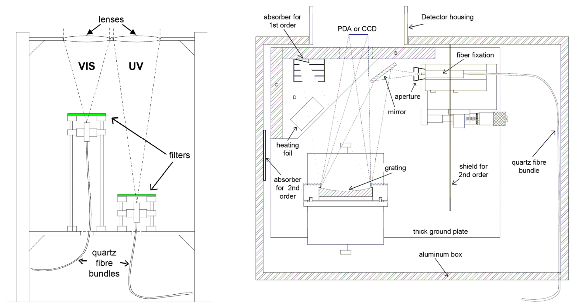
Figure A1 Entrance optics including telescope lenses, optical filters (UG5 for the UV spectrometer) and quartz fibre bundles (left). The spectrometer for the visible spectral range was operated until April 2004 and is not used in this study. Set-up of the UV spectrometer (adapted from Otten, 1997) (right).

A2 Additional fit results

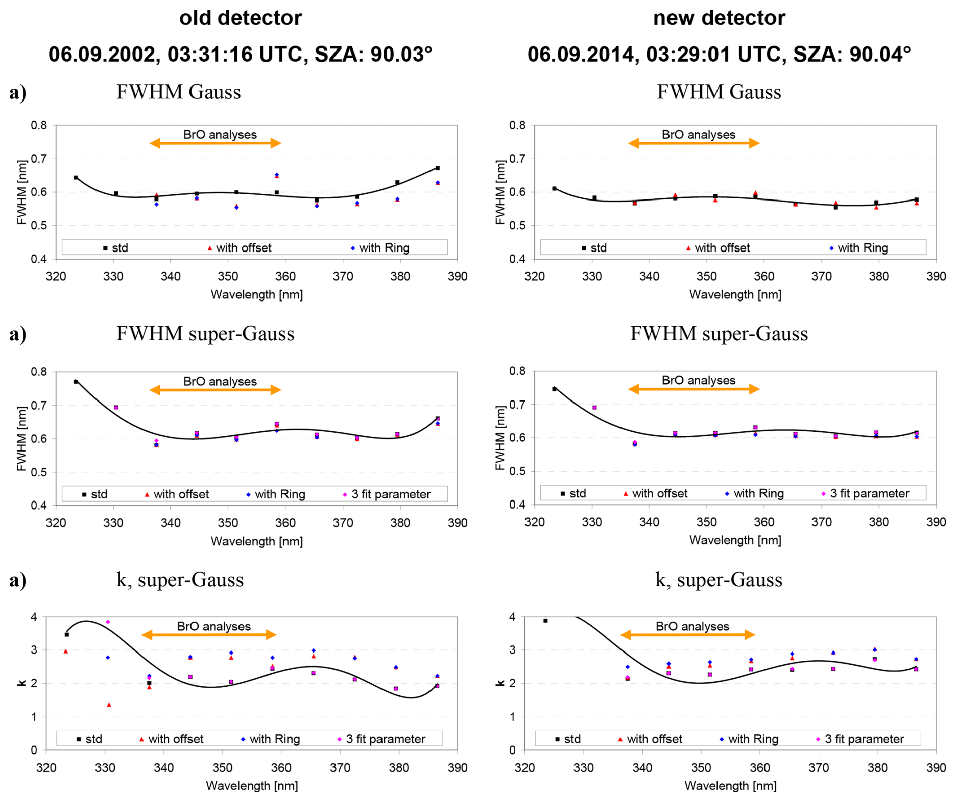
Figure A2 Same as Fig. 2, but including also a Ring spectrum or an intensity offset or for a freely fitted third fit parameter of the super-Gaussian parameterisation.

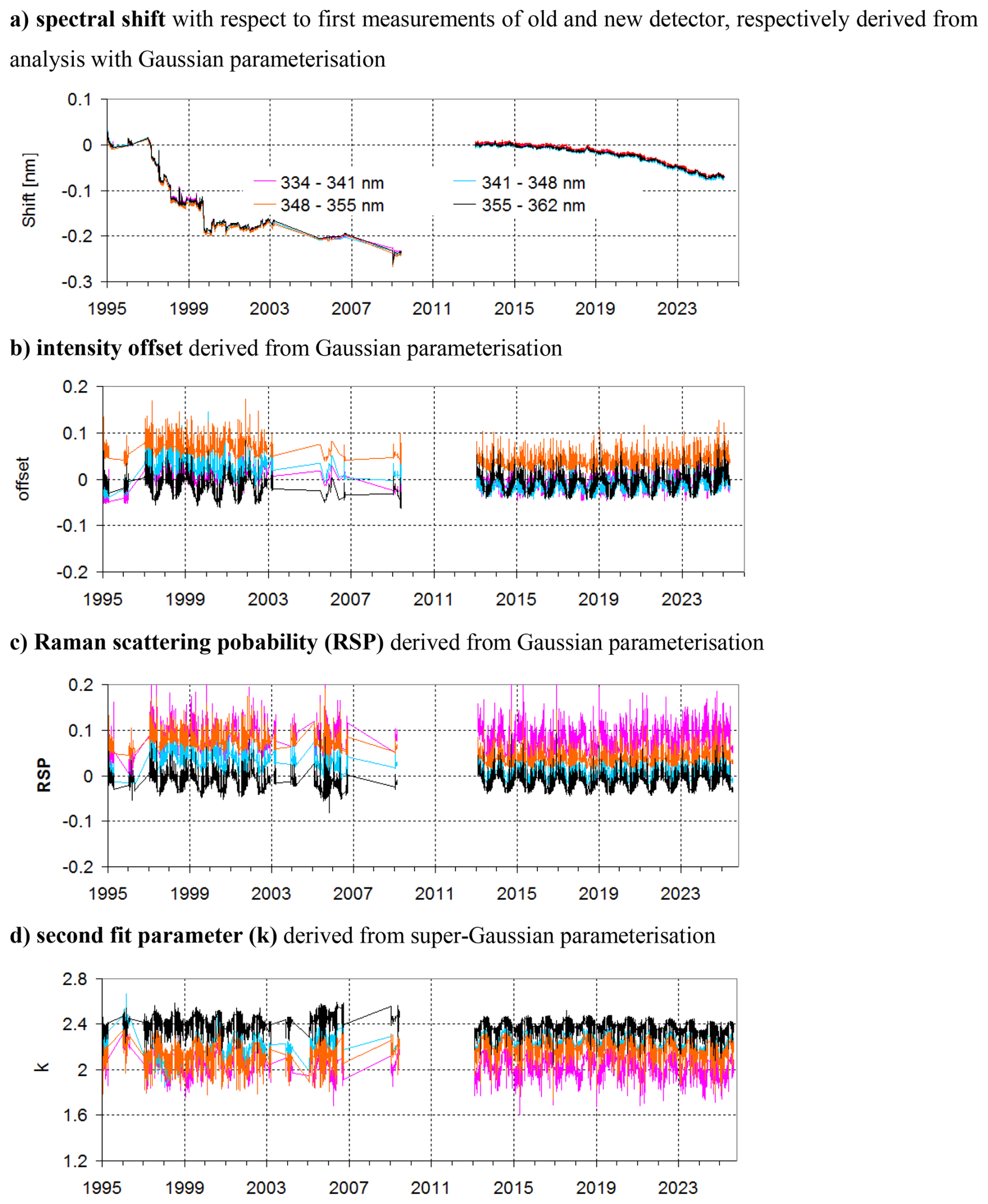
Figure A3 Time series of the further fit results determined for daily measurements (SZA between 89.5 and 90.5°) for the whole time series of the Kiruna zenith-sky measurements for 4 wavelength ranges.

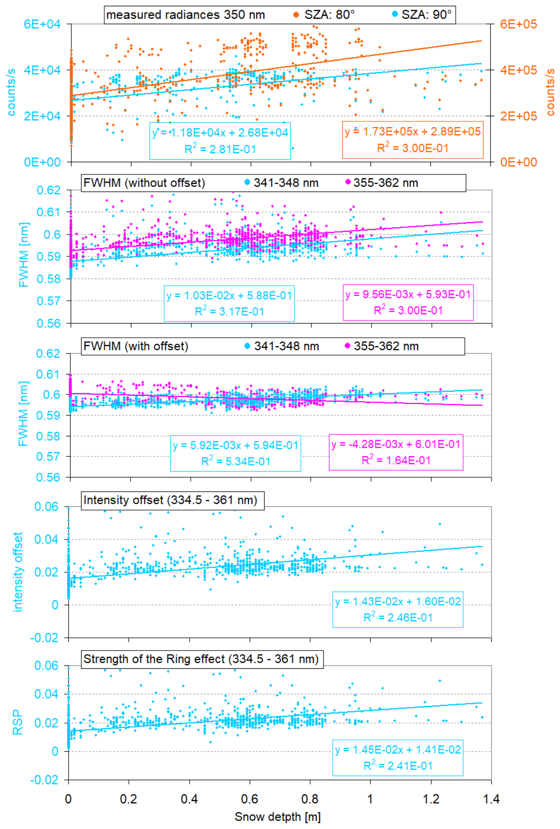
Figure A4 Correlation plots of the quantities shown in Fig. 4b to f versus the snow depth (Fig. 4a).

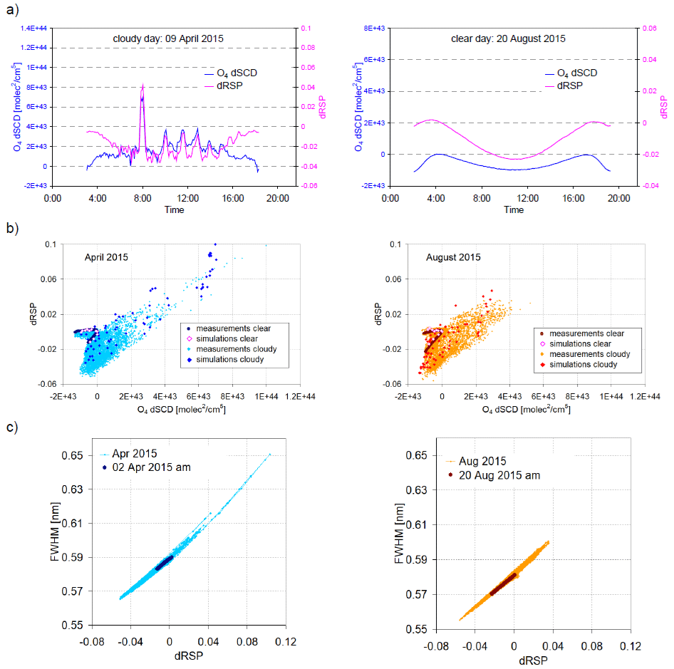
Figure A5 (a) Diurnal variation of the O₄ dSCD and strength of the Ring effect (dRSP) for a clear day (right) and a cloudy day (left). The O₄ dSCDs are analysed in the spectral range 353–387 nm. (b) Correlation plots of the dRSP and O₄ dSCD for the two selected months shown in Fig. 5. In addition, also results from radiative transfer simulations are shown. The clear sky data cover only a small part of the overall variability, which is dominated by the cloudy cases. For the radiative simulations, clouds with altitudes between 1 and 10 km and optical depths between 1 and 50 were assumed. (c) Correlation plots of the FWHM derived from the KF and the dRSP derived from the DOAS analysis for the two selected months shown in Fig. 5.

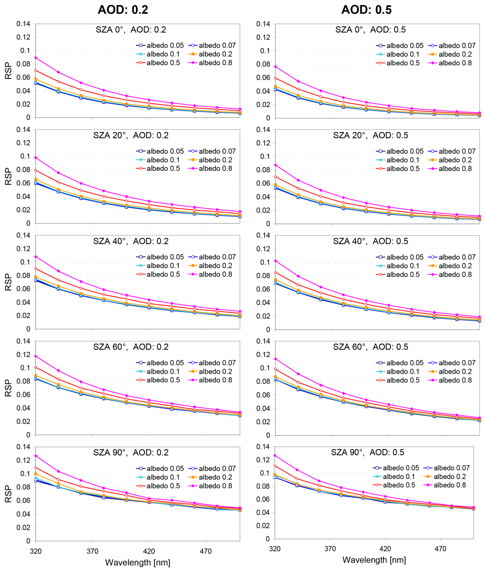
Figure A6 Dependence of the RSP on wavelength for different surface albedos, SZA and aerosol loads derived from radiative transfer simulations with the radiative transfer model MCARTIM (Deutschmann et al., 2011). The aerosol profile is assumed as box-profile from the surface to 1 km. Single scattering albedo and asymmetry parameter are set to 0.95 and 0.68, respectively.

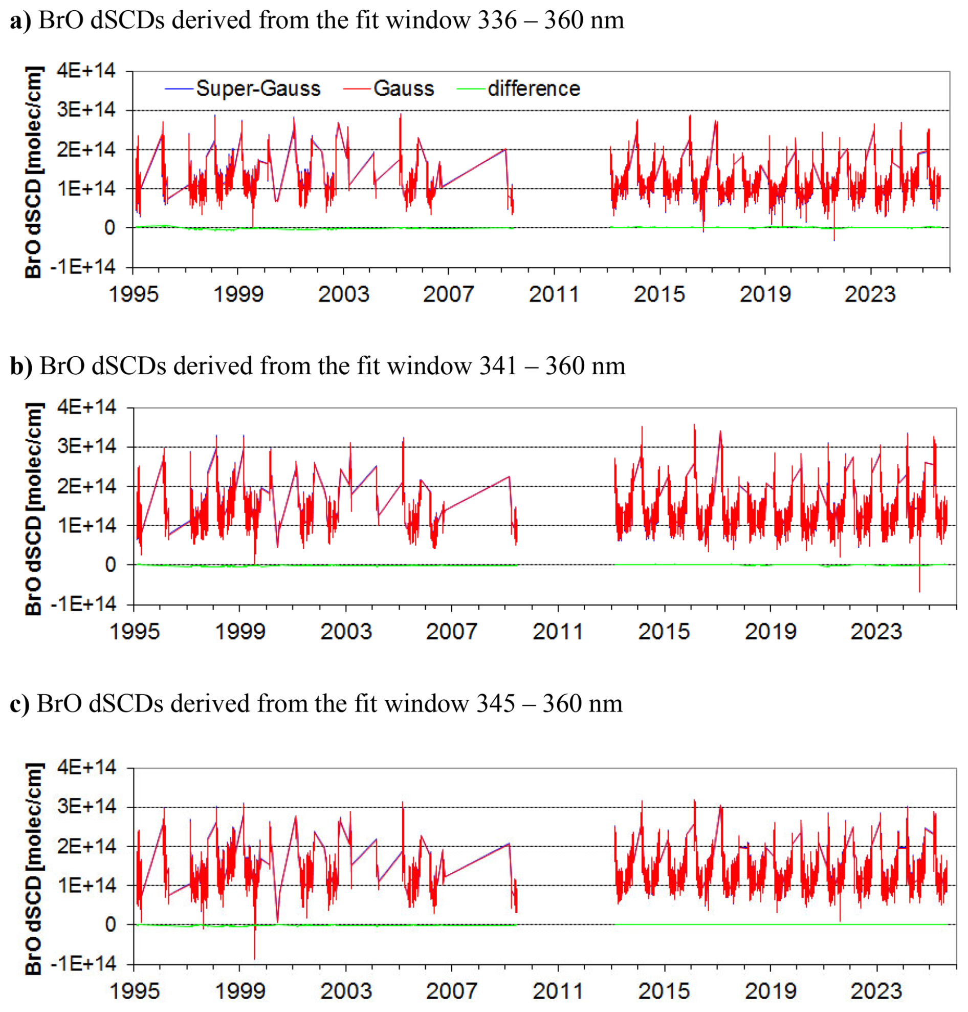
Figure A7 Time series of BrO dSCDs (90–80° SZA) obtained for different fit windows and ISRF parameterisations (red: Gauss; blue: super-Gauss). The green lines represent the differences. For both parametersiations, almost identical results are found.

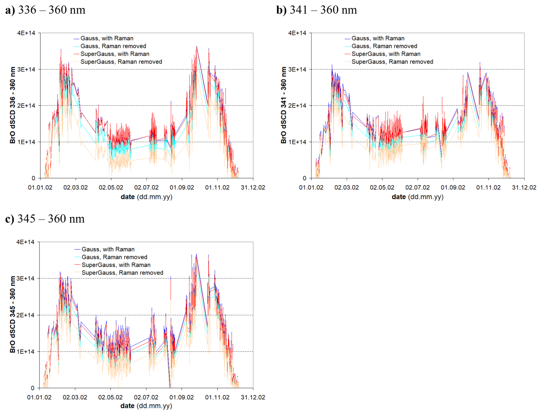
Figure A8 Retrieved BrO dSCDs (90–80° SZA) for the year 2002 using reference spectra created with different ISRF (see text).

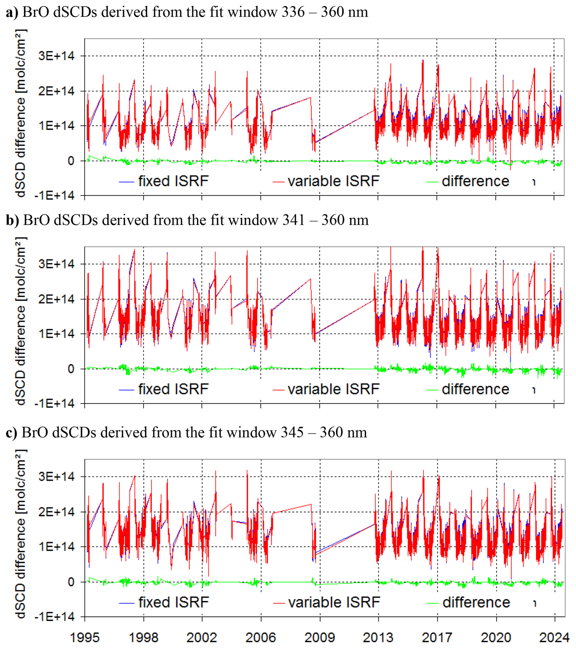
Figure A9 Time series of BrO dSCDs (90–80° SZA) for different fit windows and ISRFs (fixed or variable). The green lines represent the differences between both analyses (results with variable ISRF minus results with fixed ISRF).

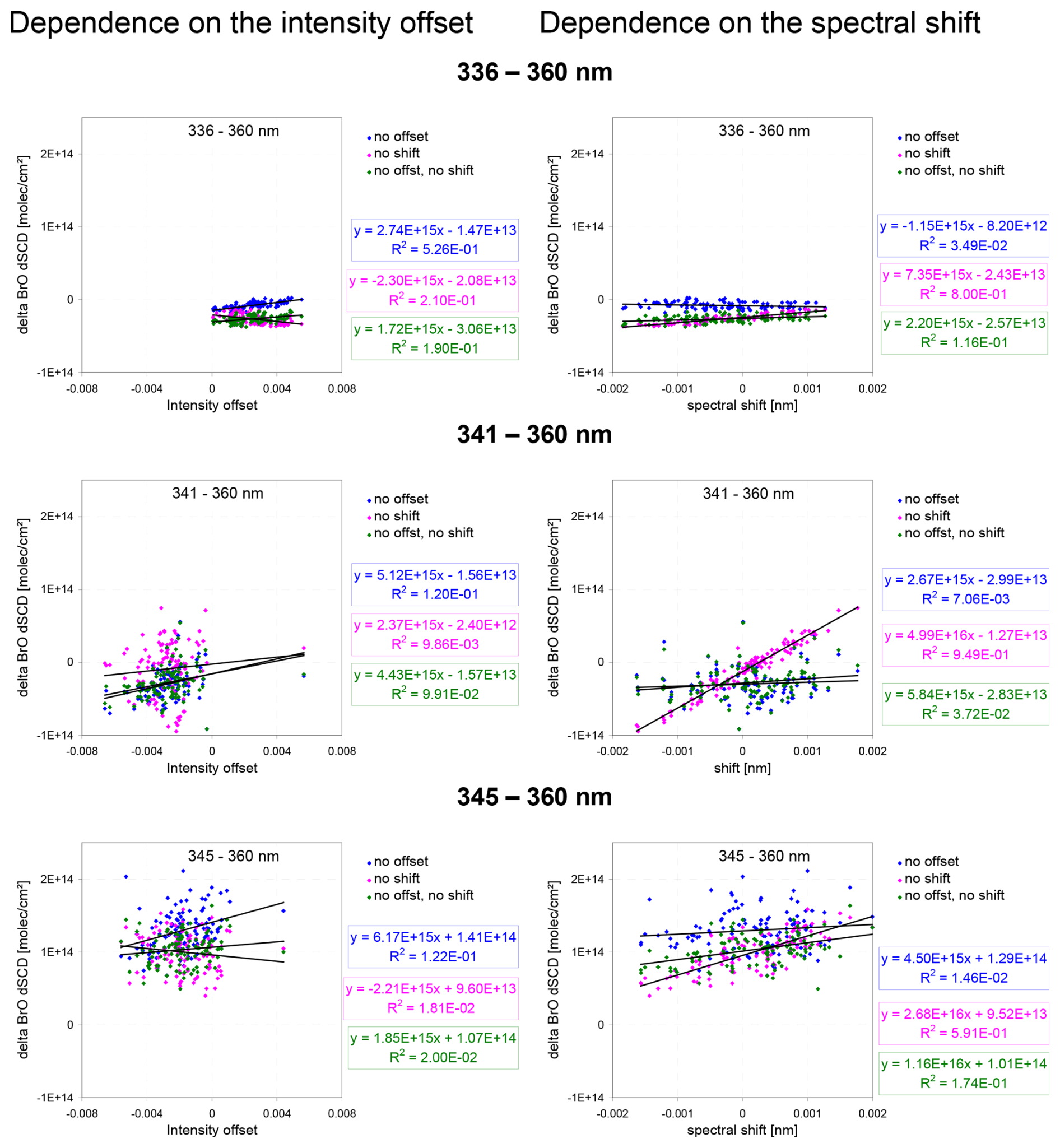
Figure A10 Correlation plots of the deviations of the BrO dSCDs from those of the standard analyses if the free fitting of a spectral shift, intensity offset, or both is deactivated versus the spectral shift (right) or intensity offset (left) derived from the standard analyses.

Figure A11 Same as Fig. 11, but for the fit ranges 334.5–360.5 and 366–392 nm.

A3 Effect of atmospheric scattering for the selected zenith measurements

In contrast to the high-resolution direct sun spectrum, the zenith-sky spectra are measurements of scattered sun light. Systematic differences between both types of measurements are caused by the effect of inelastic Raman scattering, which leads to a filling-in of the solar Fraunhofer lines (Ring effect; Grainger and Ring, 1962) as discussed in Sect. 3.3. Moreover, also the broadband wavelength dependence of both types of spectra is different because of the effects of atmospheric scattering (on molecules, aerosols and cloud particles). The measured light is attenuated by scattering processes along its way through the atmosphere. This effect is especially strong for the long light paths of the incoming direct sun light for high SZA. The attenuation is stronger for short wavelengths and leads to a “reddening” of the observed light. This reddening is counteracted by a “blueing” caused by scattering processes, which direct the sun light into the telescope of the instrument. Which process dominates the overall broadband wavelength dependence (colour) of the measured spectrum depends mostly on the SZA, but is also affected by the presence and properties of aerosols and clouds. The broadband wavelength dependence of measured spectra can be characterised by a so-called colour index (the ratio of radiances at selected wavelengths). In this study for the determination of the light throughput the wavelength pair 330 nm versus 380 nm was chosen, similar to the recommendation for the characterisation of the sky conditions (Wagner et al., 2016). But instead of 390 nm, a slightly shorter wavelength (380 nm) was chosen, which is not affected by the strong light attenuation of the optical filter (UG-5) for wavelengths above 380 nm. To quantify the absolute broadband wavelength dependence, the measured CI are compared to radiative transfer simulations for clear-sky conditions.

For the new detector a zenith-sky spectrum around 90° SZA from the first day (27 January 2013) of the measurements with the new detector was chosen. This spectrum was taken 3 d after the lamp measurement shown in Fig. 10. At the time of the measurement the sky was not (completely) clear. For the old detector a clear-sky spectrum around 90° SZA from the early phase of the permanent measurements was chosen (14 March 1997, 05:10 UTC, SZA: 90.2°). On that day, also lamp measurements are available.

In Fig. A12 the measured CI for both selected spectra are compared to simulations from the radiative transfer model MCARTIM (Deutschmann et al., 2011) for clear-sky conditions. Two aerosol scenarios were assumed: an atmosphere without aerosols and a scenario with (low) aerosol amounts in the troposphere (AOD of 0.05) and stratosphere (0.02). The results for both scenarios are almost identical for the SZA range relevant here. Thus, we conclude that the exact choice of the aerosol scenario is not critical.

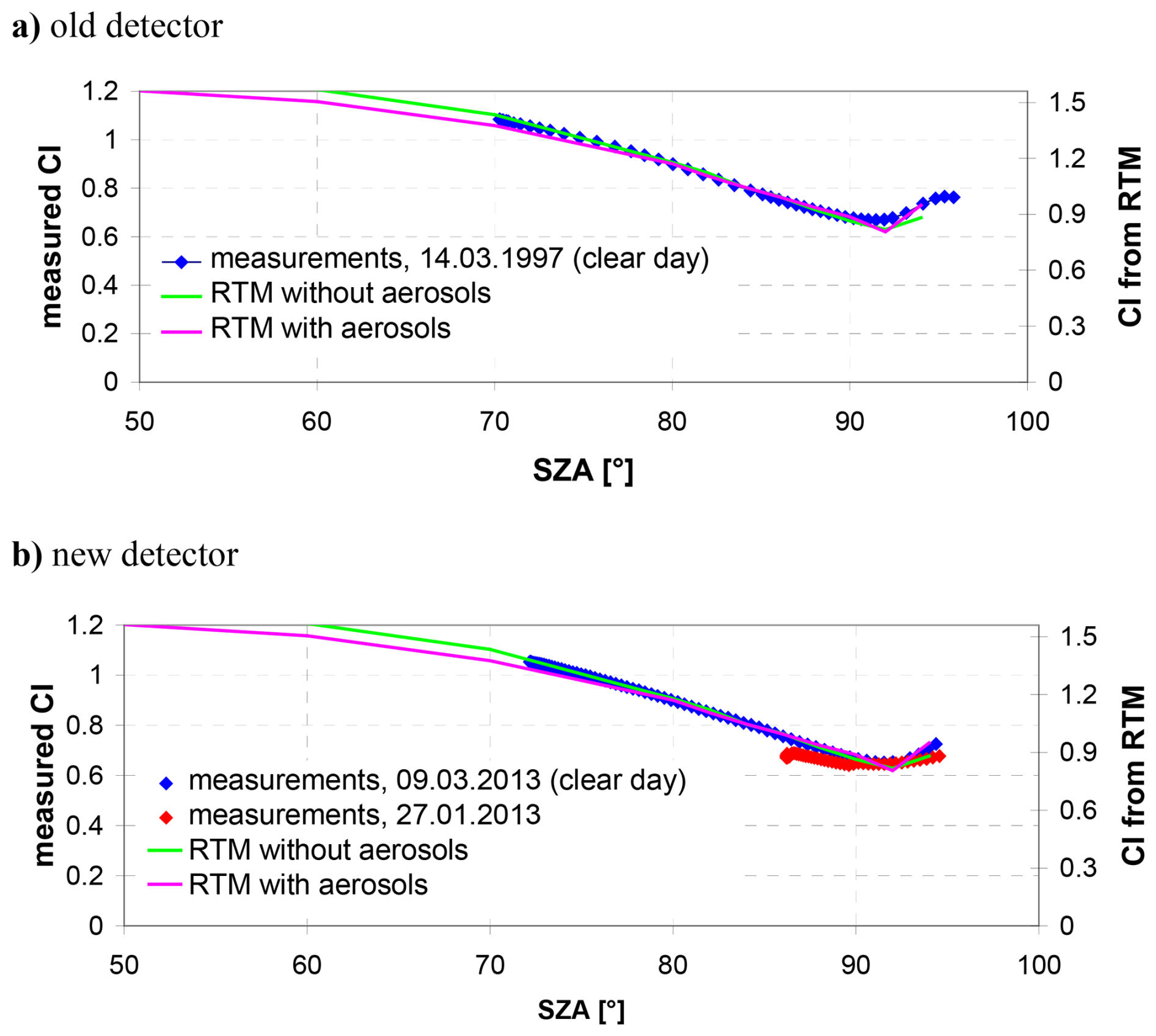
Figure A12 SZA dependence of the colour index (ratio of radiances at 330 and 380 nm) for measurements with the old (a) and new (b) detector. The blue dots represent measurements on a clear day, which can be directly compared to the radiative transfer simulations. The red dots represent measurements on a day which was affected by clouds (27 January 2013). The measured CI for this day are almost the same as for the clear day. The radiative transfer simulations were performed for two scenarios: either for an atmosphere with or without aerosols (for more details see text).

For the selected clear-sky measurements of both detectors, very good agreement of the relative SZA dependence with the radiative transfer simulations is found (the absolute values differ because of the specific instrument characteristics). For measurements around SZA of 90°, the simulated CI is close to unity (0.89) indicating that the broadband spectral dependence of the zenith-sky spectra differs from a “flat” light throughput by only about 13 % (between 330 and 390 nm). Because of the good agreement between measurements and simulations, this value can also be assumed for the selected zenith-sky spectra.