UV/Vis stratospheric air mass factors considering photochemistry at two Antarctic stations

The molecules NO₂, O₃, OClO and BrO play a major role in the photochemistry of stratospheric ozone, notably in the formation of the springtime Antarctic ozone hole. For this reason, these species have been monitored by Differential Optical Absorption Spectroscopy (DOAS) instrumentation for many decades. To transform DOAS Slant Column Densities (SCDs) into Vertical Column Densities (VCDs), independent of the viewing geometry, the Air Mass Factors (AMFs) relating these quantities are needed. Ground-based stratospheric trace gas measurements are performed in zenith-viewing geometry at twilight, around and beyond 90° solar zenith angle (SZA). At those solar angles, the Earth's sphericity and the rapid changes in photochemical parameters (e.g., photolysis rate coefficients) affect the calculation of the AMFs, particularly for photochemically active species such as NO₂, OClO and BrO. This study presents a methodology to infer AMFs that account for sphericity and photochemical effects. We estimate stratospheric AMFs of NO₂, O₃, OClO and BrO for Belgrano and Marambio Antarctic stations using the MYSTIC (Mayer, 2009; Emde et al., 2010) Radiative Transfer Model (RTM). The photochemical changes taking place during twilight are considered using a photochemical box-model based on the SLIMCAT chemistry transport model (Chipperfield, 1999, 2006). Vertical profile concentrations obtained by this model are “averaged” over the optical paths. That is, for each SZA observed at the station, a vertical concentration equivalent to all the concentrations encountered by the solar beams in different parts of the atmosphere is calculated, considering the different “local” SZAs and the partial optical paths in each layer. These concentration profiles, representative of a complete two-dimensional atmosphere, are then used as input for the one-dimensional fully-spherical version of MYSTIC RTM. The robustness of the proposed methodology is tested against measurements of NO₂, O₃, OClO and BrO SCDs obtained at Marambio Antarctic station. A good agreement is observed between modelled and measured values of NO₂, O₃ and OClO SCDs. For BrO, larger differences are obtained but they have been attributed to the tropospheric BrO contribution that has not been included in the model. Our results for Marambio 2018 show that monthly averaged AMFs can be considered as a good approximation for O₃ and BrO, but more temporally resolved sampling is recommended for NO₂ and especially OClO during July, probably due to vortex dynamics above that site. This work shows the large impact that photochemistry and Earth's sphericity can have on both the magnitude and the SZA dependence of the AMFs during twilight.

1 Introduction

Although evidence for a progressive recovery of the stratospheric ozone layer has been recently reported (WMO, 2025), the Antarctic ozone hole continues to form every year during austral spring (e.g., Solomon et al., 2014). Therefore, long-term observations of ozone and related key stratospheric trace gases such as NO₂ (e.g., Crutzen, 1979) and halogen compounds (e.g., Solomon et al., 1990; McElroy et al., 1986; Gil et al., 1996; Hendrick et al., 2007; Pinardi et al, 2022; Chong et al, 2024) remain essential. Ground-based observations performed with zenith-viewing Differential Optical Absorption Spectroscopy (DOAS) instruments (e.g., Yela et al., 2017; Yela et al., 2005) have allowed the accumulation of multi-decadal time-series of O₃, NO₂, BrO and OClO columns. OClO is formed from the reaction between BrO and ClO and can provide a good proxy for chlorine activation (Sander and Friedl, 1989).

Using the DOAS retrieval technique, differential Slant Column Densities (dSCDs) of gases absorbing in this UV-visible spectral region can be obtained:

$$\begin{array}{}\text{(1)}& \mathrm{dSCD}=\mathrm{SCD}-{\mathrm{SCD}}_{\mathrm{ref}},\end{array}$$

where SCD_ref refers to the chosen reference spectrum. SCDs represent the concentration of a given molecule integrated over the optical path of the sunlight through the atmosphere to the instrument. INTA has been operating UV-VIS DOAS spectrometers at the Belgrano (78° S) and Marambio (64° S) Antarctic stations since 1994 (Yela et al., 2017). Since 2016, both stations are part of the Network for the Detection of Atmospheric Composition Change (NDACC, https://www.ndacc.org, last access: 29 June 2026), that aims to monitor the evolution of the atmospheric composition, evaluate the impact of the observed changes, provide valuable data for satellite validation, fill in satellite data gaps and test atmospheric models. Currently, this network is composed of more than 70 stations and 160 ground-based remote sensing instruments.

During twilight, measured SCDs are mostly sensitive to the stratospheric trace gases. However, SCDs are dependent on the viewing and Sun geometry. Thus, to compare measurements performed at different times or places, SCDs are usually transformed into corresponding Vertical Columns Densities (VCDs), which are the integral of the concentration vertical profile of the considered molecule along altitude. The variable relating both quantities is the Air Mass Factor ($\mathrm{AMF}=\mathrm{SCD}/\mathrm{VCD}$ by definition). Formally, this relates to the optical definition of the AMF as described by Perliski and Solomon (1993):

$$\begin{array}{}\text{(2)}& \mathrm{AMF}=-\ln (I/I_{\mathrm{0}})/(\mathit{\sigma }\cdot \mathrm{VCD}),\end{array}$$

where I and I₀ are the intensities with and without the absorber, respectively, and σ is the absorption cross-section. In this work, we use the effective light path definition, where the SCD is the concentration integrated over the optical path. It should be noted that the equivalence between these two definitions is strictly valid for weak absorbers, where the change in intensity due to absorption does not significantly alter the radiation field (Platt and Stutz, 2008). While this approximation is appropriate for the species and spectral ranges investigated here, it could be problematic for strong absorbers, such as ozone in the short-wave UV (e.g., Rozanov and Rozanov, 2010). AMFs are a robust and well-established magnitude used for decades in many works (e.g., Perliski and Solomon, 1993; Wagner et al., 2007). They are usually computed using Radiative Transfer Models (RTM), which require an a-priori knowledge of the state of the atmosphere, i.e., vertical profiles of the different gases, temperature, pressure, etc.

Since 2012, the ground-based DOAS community working on stratospheric research (e.g., Hendrick et al., 2011; Adams et al., 2012; Yela et al., 2017), has used O₃ and NO₂ AMFs provided by NDACC (Hendrick et al., 2011). These NDACC AMFs are provided monthly in latitude bins of 10° between 85° S and 85° N and consider surface albedo equal to 0 and 1 and SZAs extending from 30 to 92° (for NO₂, AMF for 10° is also included). NDACC O₃ AMFs are computed from 440 to 580 nm in steps of 35 nm, and for NO₂ from 350 nm to 550 in steps of 40 nm, using the pseudo-spherical DISORT RTM (Kylling and Mayer, 2003). Input profiles are based on the Total Ozone Mapping Spectrometer (TOMS) v8.0 (Barthia et al., 2004) climatology for O₃ and on the Lambert et al. (1999, 2000) climatology supplemented by SAOZ balloon soundings for NO₂. NDACC O₃ AMFs consider the whole atmosphere from the surface up to the stratosphere, while for NO₂ the AMFs are exclusively stratospheric (from 12 km upward). Twilight photochemistry is neglected in NDACC AMFs.

Regarding BrO, there is little literature on stratospheric AMFs. In the recent work of Chong et al. (2024), BrO AMFs have been calculated with the Vector LInearized Discrete Ordinate Radiative Transfer Model (VLIDORT, Spurr, 2006, 2008; Spurr and Christi, 2019) using input from the Community Atmosphere Model with Chemistry (CAM-Chem) climatology (Fernandez et al., 2019), to analyse a decade of data obtained by the Ozone Mapping and Profiling Suite Nadir Mapper (OMPS-NM) onboard the Suomi National Polar-orbiting Partnership (Suomi-NPP) satellite (Flynn et al., 2014). In the work of Theys et al. (2007), Hendrick et al. (2007) and Koenig et al. (2024), BrO AMFs are used to analyse ground-based DOAS measurements from Reunion Island (21° S), Harestua (60° N) and Mauna Loa (19° N) stations, respectively. In Theys et al. (2007) and Hendrick et al. (2007), the setup applied for the BrO retrieval includes the DISORT pseudo-spherical RTM coupled with the SLIMCAT 3-D chemical transport model (CTM) and the stacked-box photochemical model PSCBOX (Errera and Fonteyn, 2001; Hendrick et al., 2004). A similar setup is used in Koenig et al. (2024) but based on the CAM-Chem model (Lamarque et al., 2012) profiles.

Regarding OClO, stratospheric AMFs are calculated in Puķīte et al. (2022) using the 3-D full spherical RTM McArtim (Deutschmann et al., 2011; Deutschmann, 2014) to analyse data from the TROPOspheric Monitoring Insrument (TROPOMI) onboard the Copernicus Sentinel-5 Precursor platform. In these studies, the AMF calculations are mostly limited to SZAs ≤90° and AMFs values are not explicitly provided. To our knowledge, the only publication showing OClO AMFs for SZA up to 95° obtained from actual measurements is Pinardi et al. (2022). In that work, ground-based DOAS instruments at 9 NDACC stations covering polar regions from both hemispheres are used to validate OClO measurements by the GOME-2 satellite instrument. Ground-based OClO values are offset-corrected using a Langley plot approach making use of empirically-derived OClO AMFs. To be more precise the AMF in Pinardi et al. is defined as the ratio of the measured slant column to the vertical column estimated at 70° of SZA, assuming that at this solar elevation a simple geometrical AMF can be used. Finally, in Kühl et al. (2004), OClO AMFs are estimated with the AMFTRAN radiative transfer model (Marquard et al., 2000) for different Gaussian vertical profiles and for SZAs between 40 and 95°.

In the present work, the stratospheric AMFs of NO₂, O₃, OClO and BrO are estimated for Marambio and Belgrano stations for SZAs (above the station) up to 94°. Photochemistry taking place during twilight is considered using a photochemical box-model based on the SLIMCAT 3-D CTM (Sect. 2.1, Denis et al., 2005; Chipperfield, 2006). Optical path averages of the concentration profiles are calculated following the method described in Sect. 2.2. Then, the AMFs are obtained by using the Monte-Carlo MYSTIC Radiative Transfer Model (RTM) (Mayer, 2009; Emde et al., 2010) (Sect. 2.3). Section 3 introduces the ground-based observations used to validate our approach. The observed AMF results are shown and compared with previous work and ground-based observations in Sect. 4. Our main conclusions are summarised in Sect. 5.

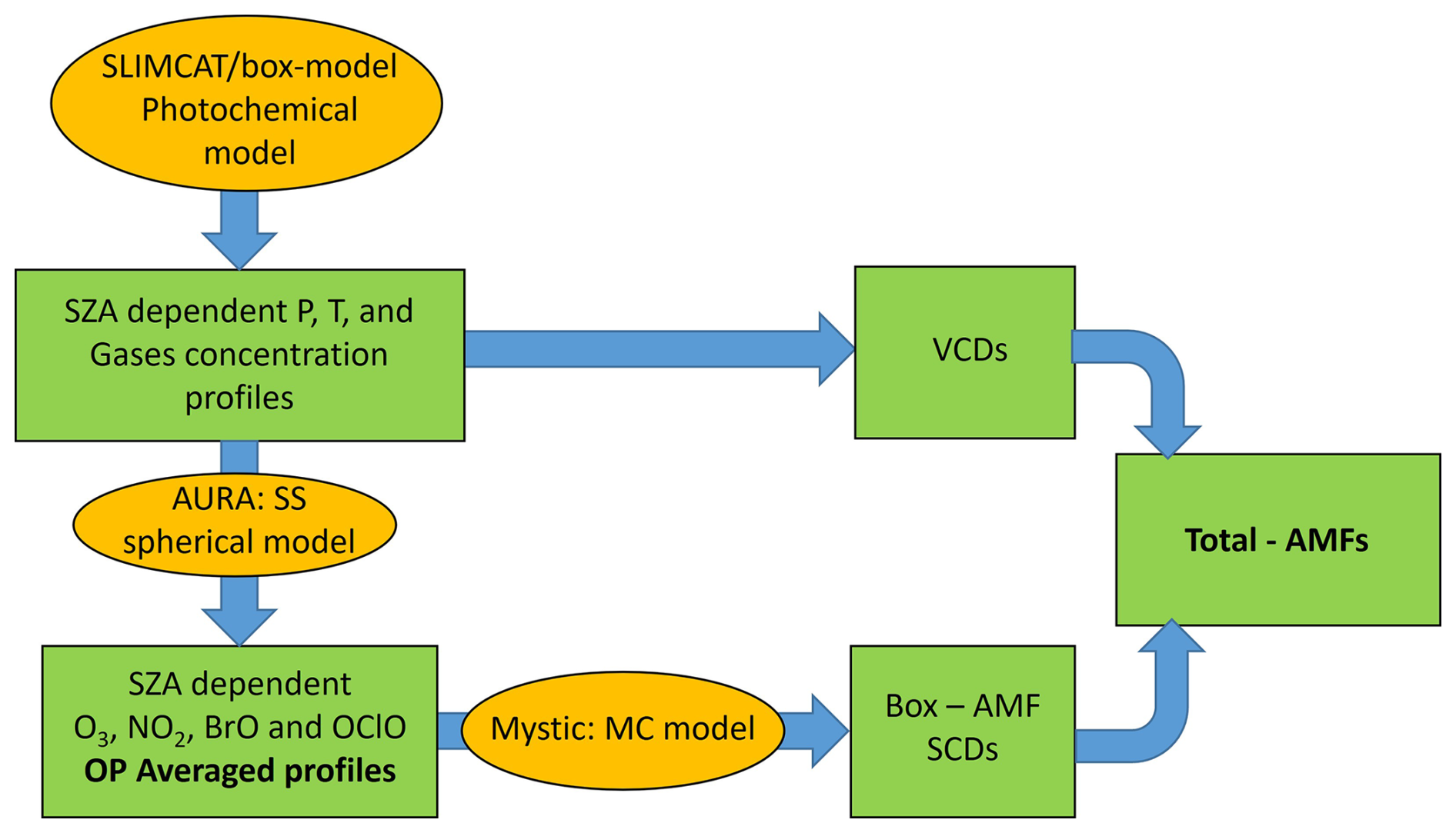
Figure 1 Summary of the AMF retrieval method. AURA (Averaged concentration estimator Using Ray-tracing Approximation) is a single scattering (SS) ray tracing model that estimates atmospheric gases concentrations averaged over the optical path (OP), (see Sect. 2.2).

2 AMF Calculation Method

The AMFs presented in this work are calculated in the UV and in the Vis spectral range: at 510 nm for O₃, 470 nm for NO₂, 351 nm for OClO and 355 nm for BrO at Marambio and Belgrano stations. The wavelengths used for O₃ and NO₂ correspond to those routinely applied in Marambio and Belgrano for NDACC retrievals. The wavelengths selected for BrO and OClO are chosen for being close to the maximum absorption of those species in the spectral range used in our DOAS measurements (see Sect. 3). We follow a four-step approach as depicted in Fig. 1:

1. In a first step, a photochemical 1-D stacked box-model coupled to SLIMCAT (Chipperfield, 1999, 2006) (see Sect. 2.1) is run with a 5 min timestep to obtain the daily SZA-dependent vertical profiles (288 SZAs per day) of O₃, OClO, BrO, NO₂, H₂O, pressure (P) and temperature (T) for Marambio and for Belgrano for a whole year. These are grouped as monthly (sunrise-am and sunset-pm) averaged profiles for SZAs from 80 to 94° in steps of 1°. The values of the SZAs at each station depend on the time of the year considered. Whenever possible, AMFs for SZA =50°, 60 and 70° are also calculated. The motivation for grouping the profiles monthly is to reduce data processing. The validity of using monthly averages versus 10 d-averaged values is evaluated in Sect. 2.2.2.

2. In a second step, (for each SZA above the station: θ) the concentration profiles obtained with the stacked box model are averaged over the SZAs encountered along the optical path for each atmospheric layer (c_l), taking into account the spherical geometry. This is described fully in Sect. 2.2.

3. Then, by using those averaged profiles as input, Box-AMFs (a_l) and SCDs are computed using the MYSTIC RTM (Mayer, 2009; Emde et al., 2010) for different SZA above the station.

4. Finally, total AMFs are calculated as explained in the following paragraph.

For each SZA above the station, box-AMFs (a_l) relate the optical path followed by sunlight at each atmospheric layer (ds_l) with the vertical layer thickness (dz_l):

$$\begin{array}{}\text{(3)}& a_{\mathrm{l}}={\displaystyle \frac{\mathrm{d}{s}_{\mathrm{l}}}{\mathrm{d}{z}_{\mathrm{l}}}},\end{array}$$

In this work, atmospheric layers of 1 km thickness have been considered from the surface to an altitude corresponding to 0.13 hPa (55–62 km, depending on the time of the year), treated here as the top of the atmosphere (TOA). From the vertical profiles of the considered gases and these Box-AMFs, the total VCDs, SCDs and the corresponding AMFs can be calculated by integrating concentration over the optical path (slant or vertical) from the surface to the TOA:

$$\begin{array}{}\text{(4)}& {\displaystyle }{\mathrm{vcd}}_{\mathrm{l}}=c_{\mathrm{l}}\mathrm{d}{z}_{\mathrm{l}},\text{(5)}& {\displaystyle }{\mathrm{VCD}}_{\mathrm{total}}={\sum }_{\mathrm{0}}^{\mathrm{TOA}}{\mathrm{vcd}}_{\mathrm{l}},\text{(6)}& {\displaystyle }{\mathrm{scd}}_{\mathrm{l}}={\mathrm{vcd}}_{\mathrm{l}}{a}_{\mathrm{l}}\mathrm{d}{z}_{\mathrm{l}},\text{(7)}& {\displaystyle }{\mathrm{SCD}}_{\mathrm{total}}={\sum }_{\mathrm{0}}^{\mathrm{TOA}}{\mathrm{scd}}_{\mathrm{l}},{\mathrm{AMF}}_{\mathrm{total}}={\displaystyle \frac{{\mathrm{SCD}}_{\mathrm{total}}}{{\mathrm{VCD}}_{\mathrm{total}\mathrm{\_}\mathrm{ph}}}},\end{array}$$

where c_l is the average concentration of the considered trace gas in each layer l, vcd_l and scd_l are the partial VCD and SCD in each layer, and SCD_total, VCD_total and AMF_total are total SCD, VCD and AMF values. Note that in all these equations, vcd_l are calculated using the averaged concentrations, but for AMF_total, we use the VCD_{total_ph} (Eq. 7) calculated from the vertical profiles obtained with the 1-D photochemical model, i.e. calculated from the vertical profiles not averaged and just above the station.

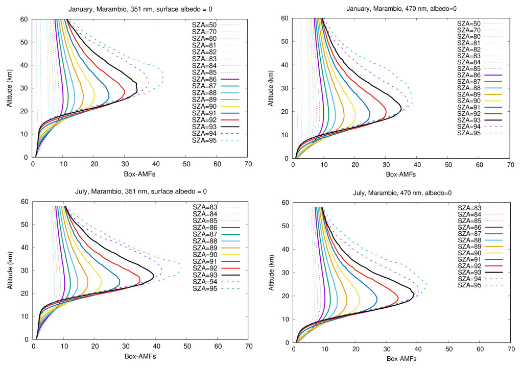
Figure 2 Box-AMFs computed for Marambio, corresponding to January (top) and July (bottom) 2018, for surface albedo =0 and different SZAs (see legend). Left panels are Box-AMFs in the UV (351 nm), right panels are Box-AMFs in the Vis (510 nm).

Figure 2 presents some examples of these Box-AMFs for Marambio with a surface albedo =0 in the UV and in the Vis. Note that, as expected for the higher SZA values, Box-AMFs below 10 km are small, due to the limited contribution of the troposphere to the optical path for this high SZA. Figure 2 shows that Box-AMFs peak at higher altitude at UV than at visible wavelengths, and the maxima of these peaks are also higher. Due to the lower attenuation of visible radiation, visible Box-AMFs extend to lower altitudes.

2.1 TOMCAT/SLIMCAT model simulations

Our analysis uses results from the TOMCAT/SLIMCAT (hereafter SLIMCAT) 3-D CTM (Chipperfield 1999, 2006). First the full 3-D model is used to perform a long-term simulation (see e.g., Dhomse et al., 2022). The model was run from 1979 to 2024 at a horizontal resolution of 2.8°×2.8° and 32 levels from the surface to around 60 km. This simulation was forced using meteorology from ECMWF ERA5 renalyses (Hersbach et al., 2020). The model has a detailed stratospheric chemistry scheme including long-lived source gases, such as CH₄, N₂O, halocarbons, and the chemical families O_x, NO_y, HO_x, Cl_y and Br_y. It also includes selected brominated and chlorinated very short-lived substances (VSLS), including CHBr₃ and CH₂Br₂. The chemistry is constrained by specified time-dependent monthly global mean surface mixing ratios of the long-lived tracers (WMO/UNEP, 2022). The two brominated VSLS both have constant tropospheric mixing ratios of 1 pptv, which together contribute a total 5 pptv to stratospheric bromine. Photochemical data used in the model is taken from NASA/JPL (Burkholder et al., 2019). In addition to gas-phase chemistry, the model includes a detailed treatment of heterogeneous chemistry on liquid sulfuric acid aerosols along with liquid and solid polar stratospheric clouds (PSCs).

Daily (00:00 UTC) outputs from the full 3-D simulation are stored for the locations of Marambio and Belgrano. This is then used as an input for daily simulations of a 1-D (stacked box) chemical model based on the same SLIMCAT chemical scheme without transport. The goal of this 1-D chemical model is to obtain the photochemical state of the atmosphere (i.e., concentrations of the different target gases) at much high temporal resolution than could be obtained directly from the 3-D model. The 1-D model is integrated each day with a 5 min timestep (meaning SZA step always lower than 0.6°) and the fields of the target gases are saved for each timestep, providing a dataset of concentrations at varying SZA for every day. The profiles at the SZAs used in our calculations are obtained linearly interpolating the photochemical model SZA values.

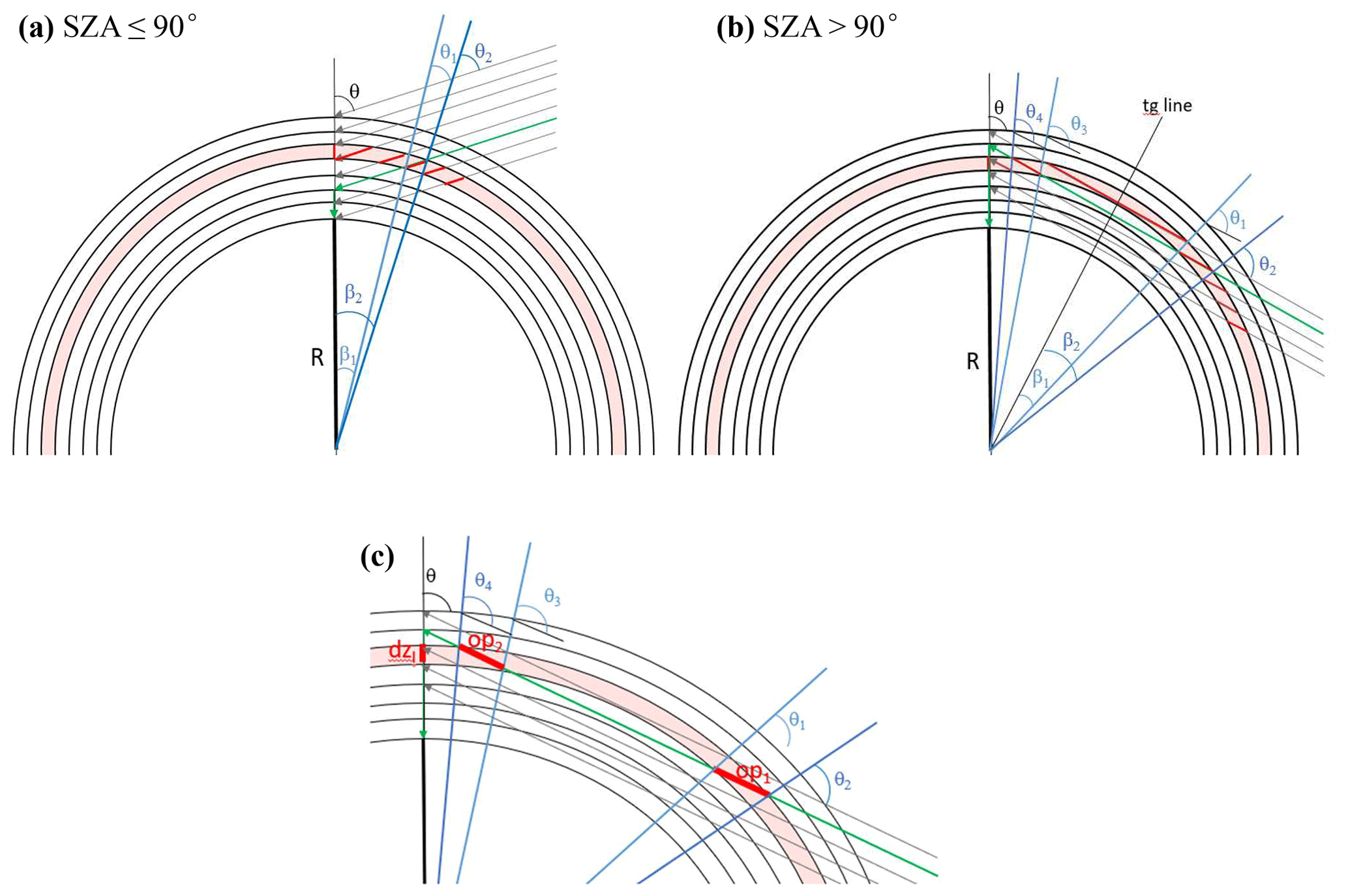
Figure 3 Schematic showing how spherical geometry is taken into account in the calculation of the averaged trace gas concentrations. Panel (a) shows the case for SZA 90° is shown. Panel (b) represents the case for SZA >90°. In panel (c) the partial optical paths for one beam and one layer are shown.

2.2 Accounting for photochemistry along the light path

The concentration profiles used in this work and provided by the photochemical model are representative for a resolution of 2.8° in latitude and longitude (the resolution of the SLIMCAT 3D-CTM). However, for large optical paths, the angle at which the solar beams reach each atmospheric layer (far away from the station) can be very different from the SZA over the station (Fig. 3), and thus the gas concentration can also differ substantially. The larger the SZA over the station, the greater the difference in the angle that each incident solar beam forms with each layer. Let (c_l,θ) be defined as the concentration of a specific gas observed by a ground-based instrument within an atmospheric layer and for a given SZA =θ. This concentration is represented as an average of the concentrations associated with all SZA values encountered by the various beams as they pass through the layer along their respective optical paths (see Fig. 3). To take this effect into account, we average the concentrations of the target species over the optical path using a ray-tracing model, AURA (Averaged concentration estimator Using Ray-tracing Approximation), developed for this purpose at INTA. There are two reasons to proceed in this way: (1) the multi-scattering Monte Carlo (MC) MYSTIC model used in this work is a 1-D model, which means that only one horizontally homogeneous vertical profile for each target species can be introduced in the model. Thus, we want to use a concentration profile representative of the whole atmosphere that takes photochemistry into account. (2) By doing this, we introduce a method that simplifies calculations and that can be used for other studies.

To average the concentrations along the light path, we make some approximations. First, we assume that solar rays are scattered only once before reaching the surface, and we divide the atmosphere into 1 km thick layers, with the top of the atmosphere (TOA) at 65 km. Note that, for an absorber above 15 km altitude and wavelengths between 350 and 650 nm, the single scattering is already a good approximation for zenith-sky stratospheric AMFs (see Figs. 2 and 3 of Perliski and Solomon, 1993). Figure 3 illustrates the geometry of the problem; panel (a) shows the optical path followed by the solar beams before reaching the surface for SZAs up to 90° at the vertical of the station; panel (b) shows the same information for SZAs >90°. In the first case, solar beams pass through each layer only once. In the second case, a solar beam can pass through a given layer once or twice slantwise and once vertically (see Fig. 3b and c). In these figures, we have labelled the SZA at which a solar beam crosses a layer as θ₁ (bottom of the layer) and θ₂ (top of the layer). Analogously, when the solar beam passes through the layer a second time, θ₃ and θ₄ are the SZAs at which the solar beam reaches the bottom and the top of the layer. Note that, when the scattering is produced above the layer considered, this layer is crossed vertically and the concentration at SZA =θ is then considered. For each SZA and each layer, the partial slant column, scd_l, can be calculated as follows:

$$\begin{array}{}\text{(8)}& {\mathrm{scd}}_{\mathrm{l}}=\sum _{\mathrm{b}}{\displaystyle \frac{I_{\mathrm{b}}}{I_{\mathrm{tot}}}}\left(\sum _i{c}_{\mathrm{b},\mathrm{l},i}{s}_{\mathrm{b},\mathrm{l},i}\right),\end{array}$$

where subscript b is for each solar beam, l is for each layer, and i is for all the partial optical paths, $s_{\mathrm{b},\mathrm{l},i}$ , and the corresponding concentrations, $c_{\mathrm{b},\mathrm{l},i}$, that each beam, b, finds when crossing the same layer, l, (red lines in Fig. 3: $s_{\mathrm{b},\mathrm{l},\mathrm{1}}=$ op${}_{\mathrm{1}},s_{\mathrm{b},\mathrm{l},\mathrm{2}}=$ op${}_{\mathrm{2}},s_{\mathrm{b},\mathrm{l},\mathrm{3}}=\mathrm{d}z$). The $c_{\mathrm{b},\mathrm{l},i}$ is obtained as the mean value between the concentration at the top of the layer and the “local” SZA at this point (θ₂ for op1 in Fig. 3c, for instance), and the concentration at the bottom of the layer for the “local” SZA at this point (θ₁ for op1 in Fig. 3c). This is true except if one beam does not reach the bottom of the layer (as optical path between op1 and op2 in Fig. 3c). In that case, the average is calculated from the values at the top of the layer and the minimum altitude reached (SZA =90°). I_b is the contribution of each beam to the total intensity, I_tot, measured at surface (Solomon et al., 1987). To simplify this, we can consider a concentration, $c_{\mathrm{b},\mathrm{l}}^{\prime }$, that is an average of all the concentrations, $c_{\mathrm{b},\mathrm{l},i}$, that a given beam experiences when crossing each layer, weighted by the ratio between the corresponding partial optical paths, $s_{\mathrm{b},\mathrm{l},i}$ , and the total optical path for that given beam and that given layer, s_b,l , (in Fig. 3: $s_{\mathrm{b},\mathrm{l}}=s_{\mathrm{b},\mathrm{l},\mathrm{1}}+s_{\mathrm{b},\mathrm{l},\mathrm{2}}+s_{\mathrm{b},\mathrm{l},\mathrm{3}}=$ op₁+ p₂+dz):

$$\begin{array}{}\text{(9)}& {\displaystyle }\sum _i{c}_{\mathrm{b},\mathrm{l},i}{s}_{\mathrm{b},\mathrm{l},i}={c^{\prime }}_{\mathrm{b},\mathrm{l}}\sum _i{s}_{\mathrm{b},\mathrm{l},i}={c^{\prime }}_{\mathrm{b},\mathrm{l}}{S}_{\mathrm{b},\mathrm{l}},\text{(10)}& {\displaystyle }{c^{\prime }}_{\mathrm{b},\mathrm{l}}=\sum _i{\displaystyle \frac{s_{\mathrm{b},\mathrm{l},i}}{S_{\mathrm{b},\mathrm{l}}}}{c}_{\mathrm{b},\mathrm{l},i},\end{array}$$

Introducing Eq. (9) into Eq. (8):

$$\begin{array}{}\text{(11)}& {\mathrm{scd}}_{\mathrm{l}}=\sum _{\mathrm{b}}{\displaystyle \frac{I_{\mathrm{b}}}{I_{\mathrm{tot}}}}{c^{\prime }}_{\mathrm{b},\mathrm{l}}{S}_{\mathrm{b},\mathrm{l}},\end{array}$$

Analogously, we now calculate the final averaged concentration for each layer, c_ave,l, as follows:

$$\begin{array}{}\text{(12)}& {\displaystyle }\sum _{\mathrm{b}}{\displaystyle \frac{I_{\mathrm{b}}}{I_{\mathrm{tot}}}}{c^{\prime }}_{\mathrm{b},\mathrm{l}}{S}_{\mathrm{b},\mathrm{l}}=c_{\mathrm{ave},\mathrm{l}}{S}_{\mathrm{l}},\text{(13)}& {\displaystyle }{c}_{\mathrm{ave},\mathrm{l}}=\sum _{\mathrm{b}}{\displaystyle \frac{I_{\mathrm{b}}}{I_{\mathrm{tot}}}}{\displaystyle \frac{S_{\mathrm{b},\mathrm{l}}}{S_{\mathrm{l}}}}{c^{\prime }}_{\mathrm{b},\mathrm{l}},\end{array}$$

where $S_{\mathrm{l}}={\sum }_{\mathrm{b}}{s}_{\mathrm{b},\mathrm{l}}$. If we now introduce Eq. (12) into Eq. (11), we have:

$$\begin{array}{}\text{(14)}& {\mathrm{scd}}_{\mathrm{l}}=c_{\mathrm{ave},\mathrm{l}}{S}_{\mathrm{l}},\end{array}$$

By doing this, we now have an averaged concentration for each SZA and each layer that represents all the concentrations found by all beams that pass through this layer.

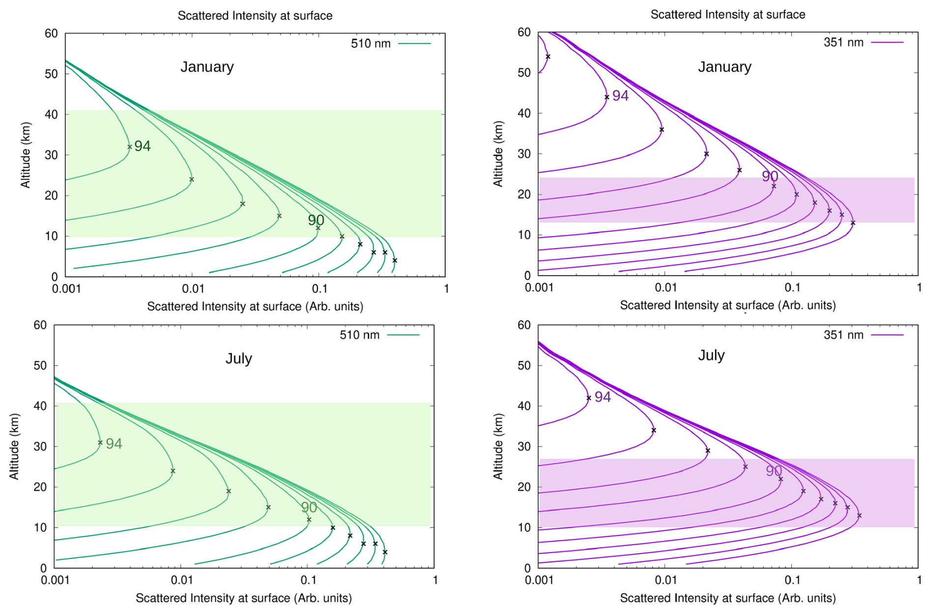
Figure 4 Scattered intensity reaching the surface for a zenith-looking instrument, as a function of the scattering altitude. Green lines (left) are the corresponding curves for the visible (510 nm) spectral range, and violet lines (right) correspond to the UV (351 nm) spectral range. Values for SZA from 85 to 94° (510 nm) and to 95° (351 nm) in steps of 1° are represented. The corresponding maxima of each of these curves (maximum scattering altitude) are represented by black crosses. Shadowed regions correspond to the altitudes where most of the O₃ or NO₂ (green) and BrO or OClO (violet) are found (from chemical model profiles used in this work). Calculations are performed for January (top panels) and July (bottom panels) 2018 at Marambio.

In some cases, the solar beam does not touch the bottom of the layer, for example see lower solar beam (grey arrows) in Fig. 3b, and the lower layer. In that case, the mean concentration is calculated between the concentration at the top of the layer and at the minimum altitude reached by the beam at that layer.

As has been indicated in the equations, the contribution of each beam to the SCD is weighted by its contribution to the total intensity observed at the surface, $I_{\mathrm{b}}/I_{\mathrm{tot}}$, (Solomon et al., 1987). In Fig. 4, the contribution of the intensity observed at the surface by an instrument looking at zenith as a function of the scattering altitude is represented for different SZAs, (the scattering altitude being the vertical distance from the instrument at which sunlight beams are scattered towards the instrument). UV solar beams are scattered towards the surface at higher altitudes compared to visible ones.

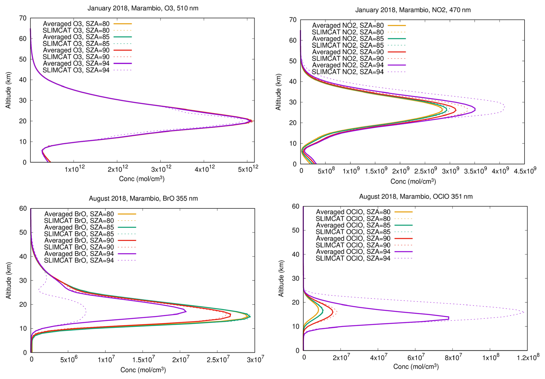
Figure 5 Comparison of vertical concentration profiles for Marambio as they are output by the 1-D chemical model above the station (dashed lines) and after averaging (solid lines) over the optical path as described in the text. Profiles for SZA =80° (above the station) are represented in yellow, for SZA =85° in green, for SZA =90° in red and for SZA =94° in violet. Top left: O₃ profiles calculated at 510 nm for January; Top right: NO₂ profiles calculated at 470 nm for January; Bottom left: BrO profiles calculated at 355 nm for August; Bottom right: OClO profiles calculated at 351 nm for August.

Figure 5 shows some examples of how the concentration profiles change after averaging their values as described above. For species such as O₃, or for low SZA for which solar beam optical paths stay close to the station, the concentration profiles do not change appreciably after averaging. However, for photochemically active species such NO₂, BrO or OClO, this can have a large impact on the profiles, especially for high SZAs. The impact of considering these averages in the final results is discussed in Sect. 3.

AURA is also able to provide the SCDs. AURA in 2-D mode calculates SCDs considering different vertical profiles for different SZAs, and AURA in 1-D mode calculates SCDs considering the same vertical profile for all SZAs. To check the validity of these approximations, a comparison between 2 set of data has been performed: (1) the SCDs of the four target species obtained using AURA in 2-D mode and considering the photochemical model concentration profiles (different for each SZA), (2) SCDs obtained with AURA in 1-D mode, using a single averaged concentration profile (Eq. 13) for the whole atmosphere. Results are almost identical (see Figs. S1–S4 in the Supplement), meaning that the calculated averaged profiles reproduce well SCDs obtained from the SZA-dependent profiles. In addition, SCDs obtained with AURA have been compared with a ray tracing model developed at BIRA that has been validated against other codes (Hendrick et al., 2006), showing similar results as AURA (see Figs. S1–S2).

2.3 MYSTIC radiative transfer simulations

MYSTIC (Mayer, 2009; Emde et al., 2010) is a fully spherical Monte Carlo (MC) radiative transfer code. Simulations performed with this code have been compared to different benchmark results (Emde et al., 2010) and other RTMs (Zawada et al., 2021) showing consistently good agreement. In MYSTIC, individual photons are traced on their random paths through the atmosphere to obtain solar-radiation-related quantities as radiances, irradiances, actinic fluxes, optical paths and Box-AMFs, for given viewing and solar geometries. Even though MYSTIC was originally conceived as a 3-D model to consider complex cloud shape (Mayer, 2009) and/or topography (Mayer et al., 2010; Schwaerzel et al., 2020), for the purpose of this work the standard Box-AMF output of 1D-MYSTIC provided in version 2.0.4 of libRadtran software package (Emde et al., 2016; Mayer and Kylling, 2005) has been used, since it is the only version available in libRadtran and clouds or complex surface topography are out of the scope of this work. An assessment of the polar stratospheric cloud effect can be found in e.g., Puķīte et al. (2022). The method used in this work does not intend to replace the powerful and straightforward 2D/3D RTM, but it provides a simplified and computationally less expensive approach accounting for photochemical changes along twilight light paths while still using 1D box-AMF calculations. Note that this study aims to systematically investigate the variability of AMFs across a wide range of SZAs, species, and timescales. Using the 1D (open source) version of MYSTIC in conjunction with our photochemical averaging allows us to maintain high vertical resolution while keeping the computational cost manageable for the large number of simulations required for this systematic study.

2.3.1 RTM settings

As explained above, O₃, OClO, BrO, NO₂, H₂O, P and T vertical profiles in our calculations are taken from the 1-D photochemical stacked box-model and averaged along the light path as explained in Sect. 2.2. Except in very rare cases when aerosols reach the stratosphere (i.e. volcanic or fire ashes), aerosols have a low influence. Thus, no aerosols are considered in our calculations. Sensitivity tests have been performed (not shown here) introducing aerosol with AOD =0.1, exponentially decreasing profile with a scale height =1 km, asymmetry parameter =0.6, and single scattering albedo =0.9. Differences in Box-AMFs with and without aerosols are less than 1 %. The solar spectrum of Kurucz (1992) is set as the solar source in our simulations. Two extreme cases of surface albedo (SA) are considered: SA =0 and SA =1. AMFs for intermediate values of SA can be estimated by interpolating between these two.

An important parameter to consider in the MC RTM is the number of photons used in the simulations. To avoid statistical instabilities in our results, we performed several calculations changing the number of photons for the different SZAs (see Fig. 6). The higher the SZA, the lower the probability of a photon reaching the ground-based instrument. Thus, the number of photons that need to be considered increases with the SZA. In our calculations, we have set the number of photons to 10⁶ for SZAs between 50 and 90°, 10⁷ for SZAs between 91 and 93°, and 5×10⁷ for SZA =94°. By using these numbers, we observe a smooth profile of the Box-AMFs in all cases (Fig. 6).

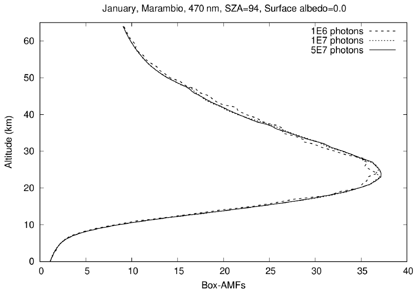
Figure 6 Box-AMFs computed for Marambio, January 2018, for SZA =94°, surface albedo =0, a wavelength of 470 nm and different number of photons: 1×10⁶ (dashed line), 1×10⁷ (dotted line), 5×10⁷ (solid line).

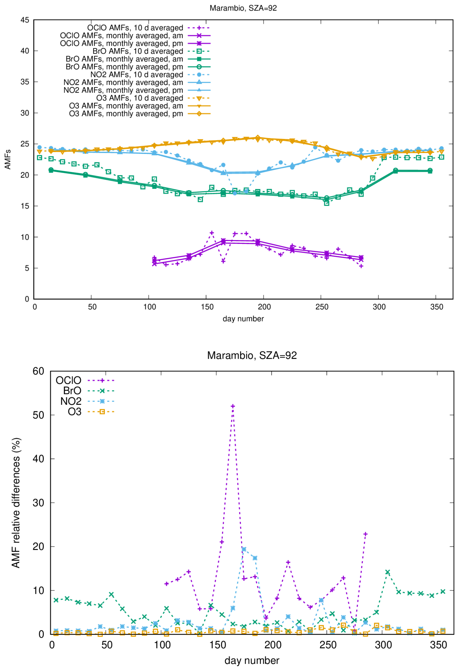
Figure 7 Top panel: OClO (violet), BrO (green), NO₂ (blue) and O₃ (yellow) stratospheric AMFs computed for Marambio 2018, for SZA =92°, and surface albedo =0. Continuous lines correspond to monthly averaged values; dashed lines correspond to 10 d averaged values. Bottom panel: Relative difference between monthly and 10 d averaged AMFs: OClO (violet), BrO (green), NO₂ (blue) and O₃ (yellow). Note that for OClO AMFs only the period in which OClO is observed is shown in the figure.

2.3.2 Temporal sampling of the AMFs

To evaluate if the use of monthly averaged AMFs is a good approximation, we have compared monthly averaged AMFs with 10 d averaged AMFs for O₃, OClO, BrO and NO₂ and for SA =0. Note that an even shorter period of time could have been chosen, daily averages for instance. However, to perform these calculations for two stations, four spectral ranges, two surface albedos and 36 time periods (10 d intervals in a year) means that the number of calculations is $\mathrm{2}\times \mathrm{4}\times \mathrm{2}\times \mathrm{36}=\mathrm{576}$ calculations with AURA and 576 with MYSTIC. Performing daily averages would mean that $\mathrm{2}\times \mathrm{4}\times \mathrm{2}\times \mathrm{365}=\mathrm{5840}$ calculations should be performed with AURA and then with MYSTIC, which is prohibitive. In addition, by performing 10 d averages, outlier values, not representative of the “normal” variability, are smoothed. Figure 7 (top panel) shows results for Marambio where, compared to Belgrano, a higher number of twilights (SZAs from 90 to 95°) are available. In the bottom panel of Fig. 7, relative differences between 10 d averages and interpolated monthly values for SZA =92° are shown. Similar results are obtained for SZA =93 and 94°, and for SA =1. The figure shows that, for Marambio, O₃ relative differences are always less than 2 %. Thus, since AMFs follow a smooth temporal variability, using monthly values can be considered as a good approximation. Maximum relative differences for BrO are below 7 % most of the year, except during summer where these differences increase up to 14 %. We conclude that monthly values are still a reasonable approximation. Also, for NO₂, relative differences are below 8 % except during the month of June (minimum in NO₂) when the differences reach 19 %. In contrast, OClO AMFs at Marambio show a high temporal variability during the chlorine activation period, probably linked to vortex dynamics above this site. Thus, if the goal of using the AMFs is to reveal annual or inter-annual variability, the use of monthly averages is justified. However, taking into account that for individual measurements these differences are expected to increase, for the study of specific episodes (a few days), daily sampling is recommended specially for OClO at stations close to the vortex edge as Marambio.

3 Ground-based DOAS observations

The measurements used for the validation of our AMF calculation approach rely on ground-based MAX-DOAS instruments (Platt and Stutz, 2008) operated at the Antarctic stations of Marambio (64°13^′ S, 56°37^′ W) and Belgrano II (77°52^′ S, 34°7^′ W). At each of these sites, INTA has deployed MAX-DOAS systems operating in the visible and UV spectral ranges (for O₃/NO₂ and BrO/OClO, respectively). At SZA <85°, these instruments perform vertical scans of the atmosphere with small telescopes moving from the horizon to the zenith, capturing scattered skylight. During morning and evening twilights, the telescopes are fixed in zenith-viewing geometry to focus on the measurement of stratospheric gases such O₃, NO₂, BrO and OClO. Details on the design of the instruments can be found in Prados-Roman et al. (2018) and Gomez-Martin et al. (2021). Spectral radiance data are analysed using INTA's analysis software LANA (Gil et al., 2008; Peters et al., 2017). NO₂ is processed in the spectral range 425–490 nm (Kreher et al., 2020), O₃ in 450–534 nm (Hendrick et al., 2011), BrO in 346–359 nm (Aliwell et al., 2002), with updated cross-sections: O₃: Serdyuchenko et al. (2014); O₄: Finkenzeller and Volkamer (2022), OClO: Kromminga et al. (2003), OClO in 345–389 nm (Pinardi et al., 2022). Measurements used in this work refer to observations performed in 2018.

Table 1 Models and concentration profiles referred in this work and used in Figs. 8 to 11.

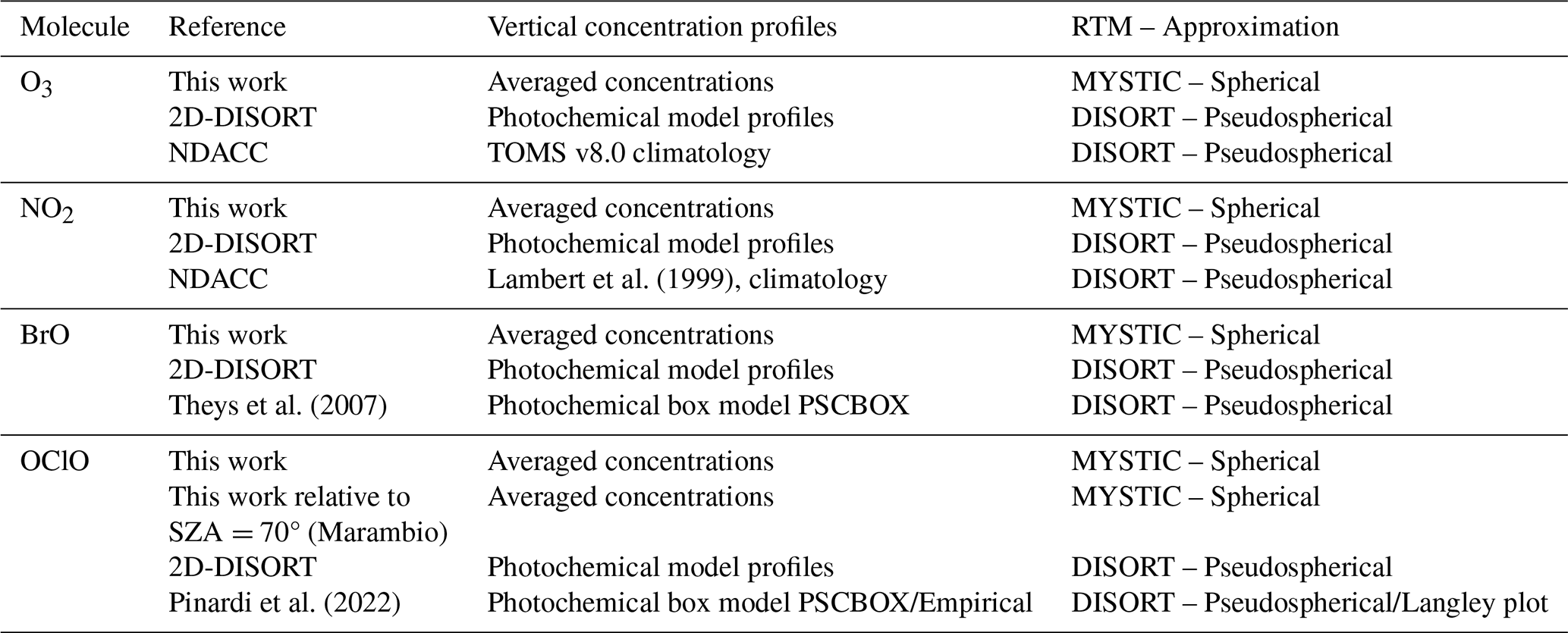
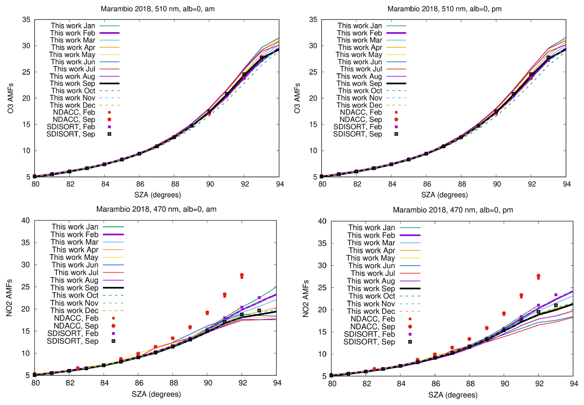
Figure 8 Total Visible AMFs: O₃ (top row), NO₂ (bottom row) computed for Marambio 2018, for surface albedo =0: Sunrise values at left and sunset values at right. Red symbols correspond to NDACC AMFs for O₃ and NO₂ (Hendrick et al., 2011). 2D-DISORT AMFs for February (violet crosses) and September (black squares) are also shown.

4 Results

4.1 AMF calculations for O₃, NO₂, BrO and OClO

Applying the method described in Sect. 2, stratospheric AMFs were calculated for the four target species O₃, NO₂, OClO and BrO. Results for surface albedo =0 are shown in Figs. 8 and 9 for Marambio, and Figs. 10 and 11 for Belgrano. Differences between AMFs calculated for albedo =0 and albedo =1 are very small (i.e., for 90° SZA, less than 0.8 % for O₃ and NO₂, up to 2 % for BrO and 3 % for OClO for September). The values of the AMFs calculated in this work are provided in the Supplement. The validity of our calculations in the Vis spectral range is tested by comparing our O₃ and NO₂ AMFs with those from NDACC which have been used since 2012 as a reference for the DOAS scientific community (e.g., Hendrick et al., 2011; Yela et al., 2017). The validity of our UV results is evaluated by comparing them with data available from the literature (Theys et al, 2007; Pinardi et al., 2022). For SZAs up to 93°, our results are also compared to AMFs obtained with the pseudo-spherical 2D-DISORT (Hendrick et al., 2004) (2D refers to using different vertical profiles for different SZAs). This comparison, which addresses both UV and visible AMFs, is restricted to albedo =0, since large differences are not observed in the AMFs for other albedo values. All the data used in Figs. 8 to 11 are included in Table 1.

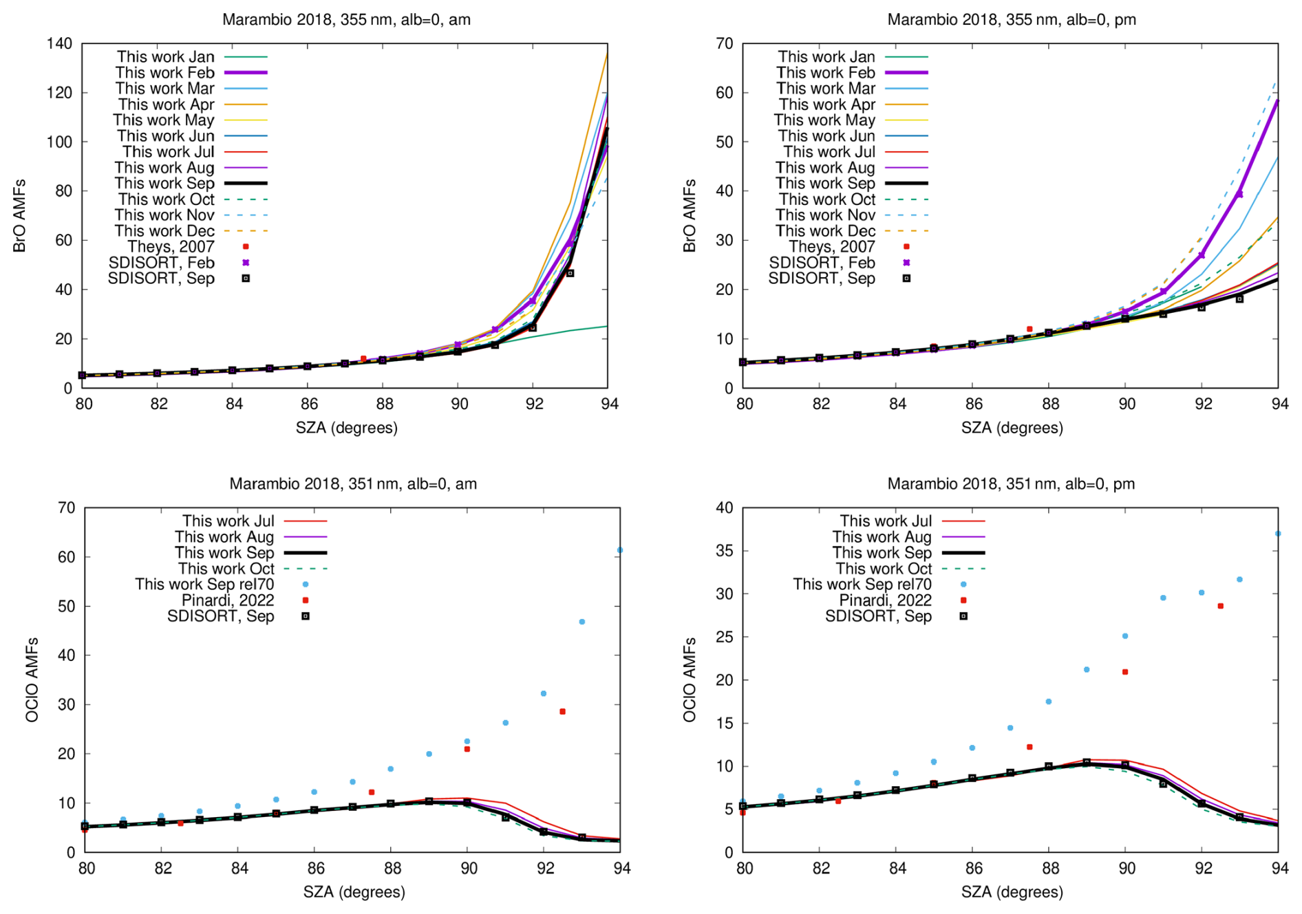
Figure 9 Total UV AMFs: of BrO (top row), OClO (bottom row) computed for Marambio 2018, for surface albedo =0: Sunrise values at left and sunset values at right. OClO AMFs from Pinardi et al. (2022) and BrO AMFs from Fig. 2 of Theys et al. (2007). 2D-DISORT AMFs for February (violet crosses) and September (black squares) are also shown.

In Fig. 8, for O₃ and NO₂ our results have been cross-checked with the February and September O₃ and NO₂ AMFs used for NDACC (red dot symbols in the figures), for the same surface albedos and wavelengths and for a latitude of 65° S (close to the latitude of Marambio) (Hendrick et al., 2011). In Fig. 10, our O₃ and NO₂ results for Belgrano have also been cross-checked with the February and September O₃ and NO₂ AMFs used for NDACC (red dot symbols), for the same surface albedos and wavelengths, and for a latitude of 75° S (close to the latitude of Belgrano). In the same figures, 2D-DISORT AMFs for the same example months (February: violet dots; September: black dots) are also shown. As SZA =90° is the value used to report VCDs within NDACC, we discuss results using the AMF values at this SZA as reference.

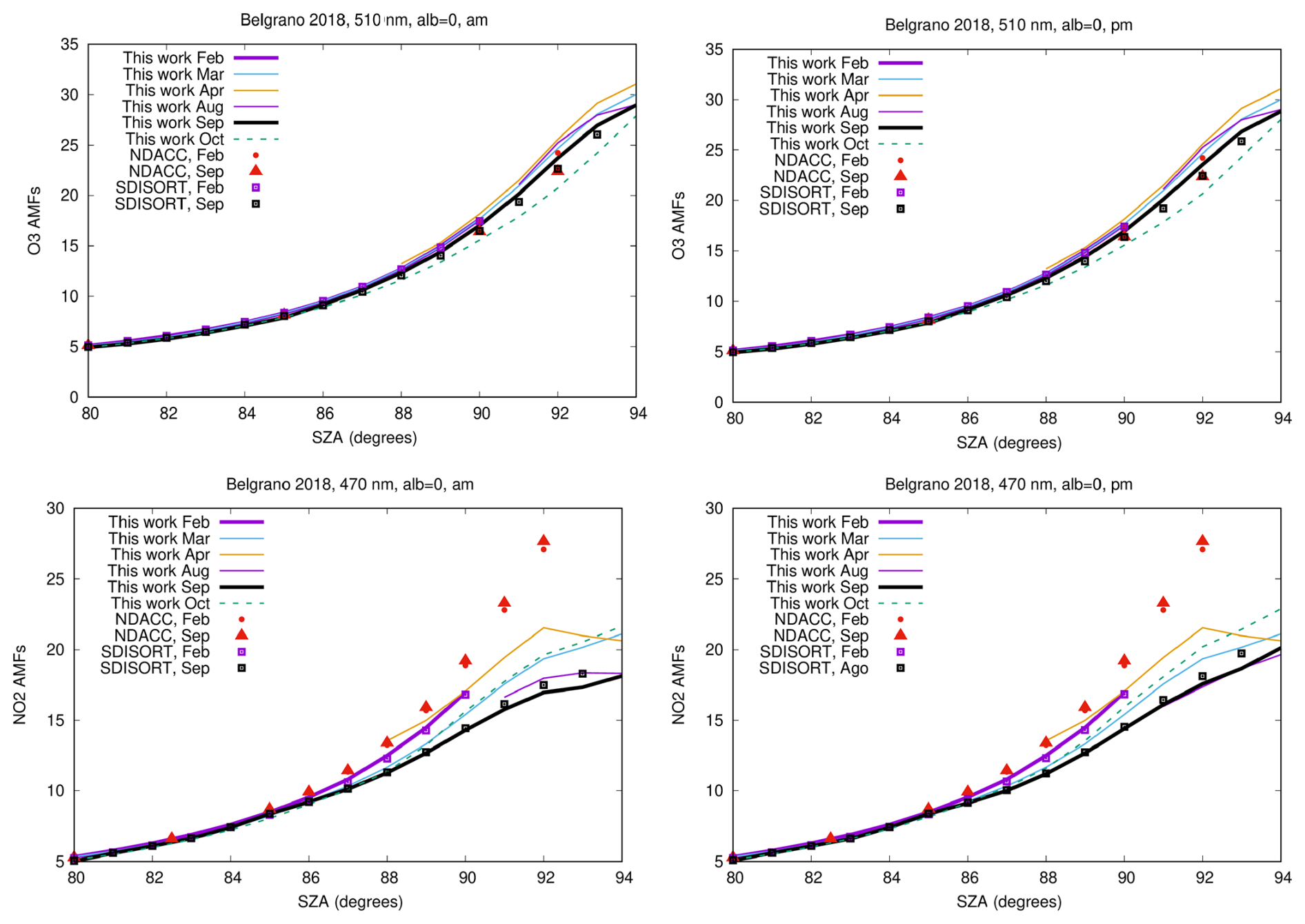
Figure 10 Total Visible AMFs: O₃ (top row), NO₂ (bottom row) computed for Belgrano 2018, for surface albedo =0: Sunrise values at left and sunset values at right. Red symbols correspond to NDACC AMFs for O₃ and NO₂ (Hendrick et al., 2011). 2D-DISORT AMFs for February (violet squares) and September (black squares) are also shown.

For O₃ at Marambio, our results are similar to NDACC as well as 2D-DISORT values, showing maximum relative differences of 1.8 % (NDACC) and 0.6 % (2D-DISORT) larger AMFs for September, with even smaller differences for February. However, these differences increase up to −26 % when comparing NO₂ AMFs from this study with NDACC data, while the difference with 2D-DISORT simulations remains low (1.2 %). Regarding Belgrano, our results for O₃ show differences with NDACC always below 3.5 % and the same with 2D-DISORT values. For NO₂ these differences increase with SZA up to −29.0 % for NDACC and remain below 1.0 % for 2D-DISORT. To better understand the origin of these deviations, we consider the differences between the methods used to obtain these different data sets. First, pseudo-spherical RTM have been used for NDACC and 2D-DISORT AMFs in contrast with the fully spherical RTM used in this work. However, given that DISORT and MYSTIC are providing similar results (see Figs. 8–11 and S5), this geometrical difference cannot explain the observed differences. Concerning vertical profiles, NDACC AMFs use the TOMS v8.0 (Barthia et al., 2004) climatology for O₃, and Lambert et al. (1999, 2000) climatology in combination with SAOZ balloon soundings for NO₂ as vertical profiles of these molecules, provided for latitudes from 85° S to 85° N in steps of 10°. Twilight photochemistry and optical path averages taken into account in this work are not considered in the NDACC AMF calculation. In the case of 2D-DISORT and MYSTIC, outputs of the photochemical model described in Sect. 2.1, specific for 2018, considering a region of 2.8° around the station, are used directly (DISORT) or averaged to obtain equivalent concentration profiles accounting for photochemistry (MYSTIC). That means that the geographical region considered in this work is significantly smaller than the latitude belt (10°) considered for NDACC. In addition, the concentration profiles used in this work are specific for the year 2018, while NDACC AMFs use climatological data published 25 years ago. Therefore, this seems to be the most probable factor causing the observed differences is the different concentration profiles considered in each set of data.

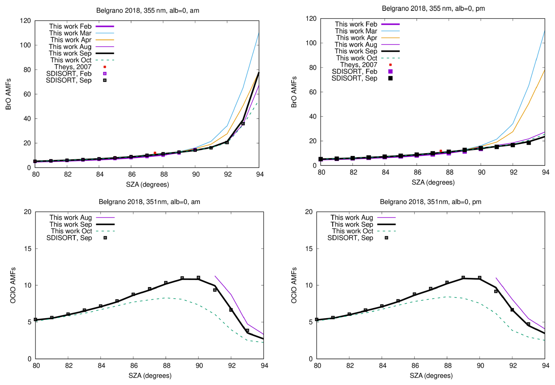
Figure 11 Total UV AMFs: of BrO (top row), OClO (bottom row) computed for Belgrano 2018, for surface albedo = 0: Sunrise values at left and sunset values at right. BrO AMFs from Fig. 2 of Theys et al. (2007) (red dots) and 2D-DISORT AMFs for February (violet squares) and September (black squares) are also shown.

For species like O₃, whose composition and distribution with altitude do not suffer large variation during twilights, these differences do not have a large impact on the results as can be seen in Fig. 8. For other species with larger variations in their vertical profiles during twilight (e.g., NO₂), the differences in AMFs are more important. This fact is of special relevance for the short-lived molecules BrO or OClO. In this case, there are very few AMF values available in the literature for comparison. In Figs. 9 and 11, we compare our results with those of Pinardi et al. (2022) for OClO, and Theys et al. (2007) for BrO. Note that for BrO, we have not found any published reference of the AMFs for SZA higher than 90°. In both cases, we have also compared MYSTIC with 2D-DISORT calculations. In the work of Pinardi et al. (2022), AMFs are obtained as the ratio between SCDs for different SZAs and the VCD at SZA =70°. To properly compare our results with those of Pinardi et al. (2022), AMFs referred to VCD =70° for September have also been included in Fig. 9 as blue dots. Differences in both sets of data are of 7 % for sunrise and 18 % for sunset (both at SZA =90°). Note that the evolution of the concentration profiles of photochemical species can be very different for sunrise and sunset, especially for high SZAs (see Fig. 12). However, in Fig. 9 the Pinardi et al. (2022) AMFs are empirical averaged (am–pm) values, corresponding to the AMFs provided to the several groups participating in that work. In contrast to other species, for which AMFs increase with SZA, the stratospheric OClO AMFs obtained in this work show a local minimum close to SZA =93° for most of the year, also observed in Kühl et al. (2004). This results from the strong increase of the OClO concentrations beyond 90° SZA. Comparisons with 2D-DISORT simulations show absolute differences lower than 0.5 for Marambio, and 0.3 for Belgrano. For BrO, both 2D-DISORT and MYSTIC present an important increase of the AMFs with SZA, due to the strong decrease of the BrO concentration beyond 90° SZA in this case. Note that in the visible spectral range, the maximum scattering altitude ranges between 12 and 42 km for SZA between 90° and 95° (see Fig. 4). This coincides with the bulk altitude of both O₃ and NO₂ concentrations (see Figs. 4 and 5). In the UV spectral range, the maximum scattering altitude ranges between 22 to 54 km for SZA (see Fig. 4), while the bulk of the OClO and BrO concentrations is located between 10 and 25 km (see Figs. 4 and 5), i.e., mostly below the scattering altitude. However, while OClO increases at low Sun and essentially remains in the same altitude range, BrO decreases and its maximum concentration moves towards higher altitudes, where the main scattering takes place (see Fig. 12). This fact was already observed in the work of Perliski and Solomon (1993).

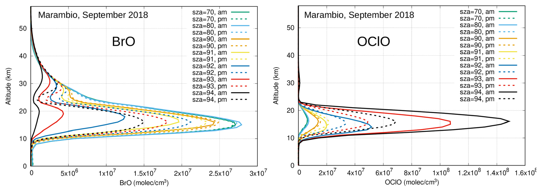
Figure 12 Evolution with SZA of the concentration of BrO (left) and OClO (right) over Marambio during September 2018. Concentration profiles have been obtained with the photochemical model based on SLIMCAT.

There is also another factor contributing to these differences in AMF behaviour between the various species. When photochemistry is not considered, the only factor changing with the SZA is the optical path that increases with the SZA. However, when photochemistry is considered, not only does the optical path change but also the vertical profile of the species (1) different profiles occur for different SZAs over the station, and (2) for each of these SZAs over the station, different profiles along the optical paths of the Sun beams. As the AMF is the ratio between the SCD and the VCD, the value of the AMF depends on the evolution of the VCD and SCD, which are influenced not only by the optical path but also by the changing concentration profile. Note that, when calculating the SCD average, we consider the concentration vertical profiles observed across the optical path, with SZA increasing up to the SZA above the station (see Fig. 4). These paths experience a lower SZA, corresponding to lower concentrations of NO₂ and OClO but higher concentrations of BrO (see Fig. 5). Thus, when the SZA increases, the SCD averaged over the optical path is lower than the SCD (obtained with the photochemical model) for the SZA just over the station for NO₂ and OClO and higher for BrO. As already noted, this also contributes to the evolution observed in the twilight AMFs of these molecules.

All of the features explained above are also applicable to the Belgrano station (see Figs. 10 and 11). In this case, the number of months for which the sunlight reaches our instrument is smaller than for Marambio, thus the number of AMFs is also smaller. However, the behaviour of the monthly mean AMFs is similar to that observed at Marambio.

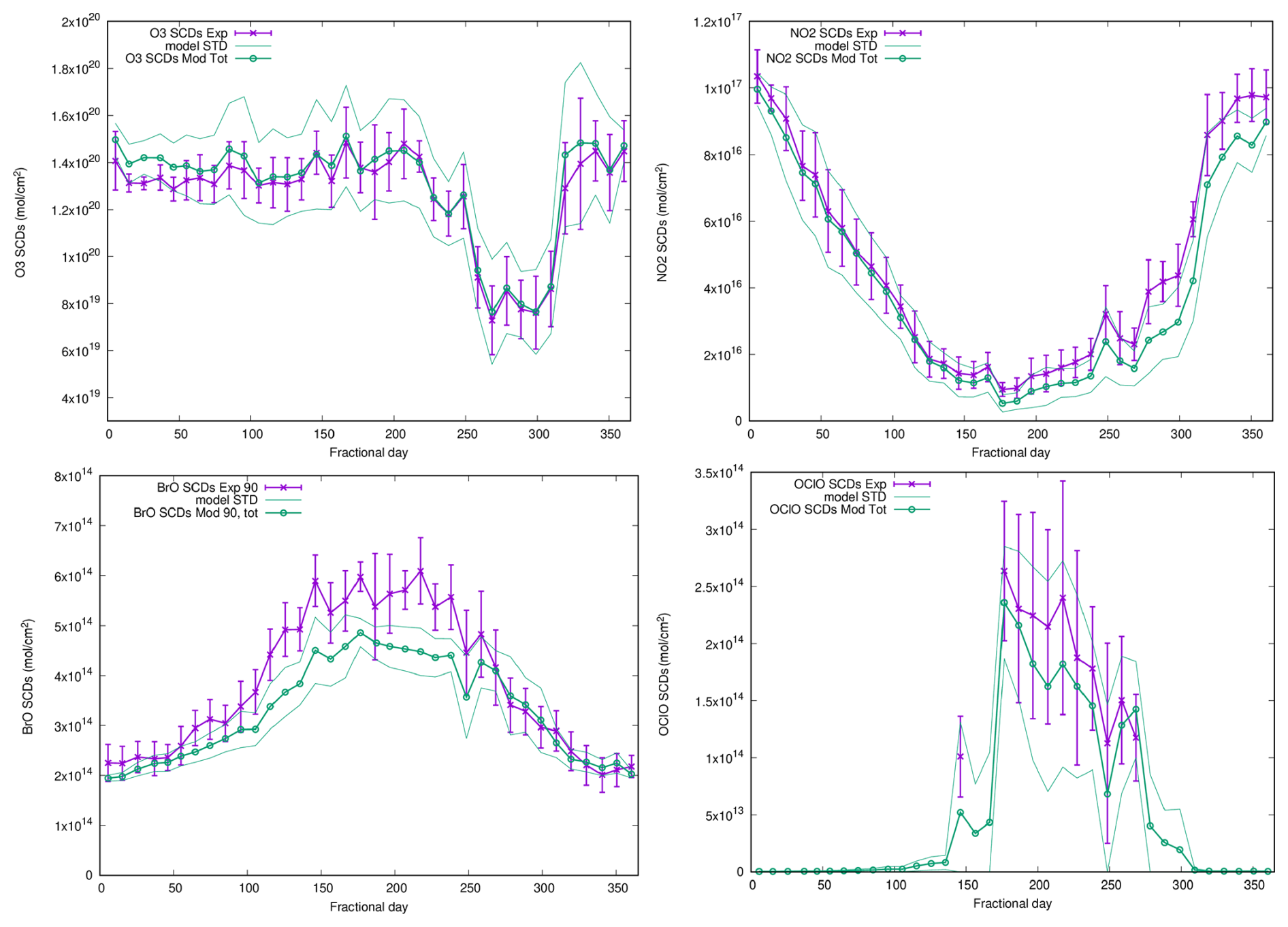
Figure 13 Measured (violet) and modelled (green) O₃ (top, left), NO₂ (top, right), BrO (bottom, left) and OClO (bottom, right) SCDs for Marambio 2018, and SZA =90°. For a given 10 d period, the photochemical model provides 2 profiles per SZA per day (am and pm), i.e. 20 profiles for a whole 10 d period. The mean profile and its standard deviation for each 10 d period are calculated. In this figure, the green dots represent the SCD obtained with the mean profiles, and the fine green lines the SCDs obtained with the mean profile plus/minus the standard deviation of the profiles.

4.2 Comparison with measurements

To further verify the validity of our results, experimental SCDs obtained in 2018 using INTA ground-based DOAS instrument in Marambio have been compared with modelled SCDs (see Fig. 13). Note that for OClO, the detection limit is about 1.0×10¹⁴ molec. cm⁻², thus measurements below this detection limit have not been included in the figure. We have compared SCDs calculated and measured at SZA =90° since that SZA is a good compromise in terms of instrumental signal-to-noise ratio for twilight observations. Similar results (not shown) have been found for SZA =92°. For comparison, experimental and modelled SCDs have been averaged in a 10 d period and represented in the middle of the period considered. Error bars of experimental data represent the standard deviation of all the points used in the average. Modelled SCDs are obtained from the calculated Box-AMFs, considering photochemistry, Earth sphericity and the optical path averages described in previous sections. In practice, the analysis of measured spectra provides differential SCDs (dSCDs) against a given reference (see Sect. 3). This reference is usually selected for conditions at which the contribution of the SCD of the target trace gas is a minimum. When studying stratospheric SCDs, the reference is also chosen to minimise the possible contribution from tropospheric absorbers. For the case of interest in this work, these conditions are met at the beginning or at the end of the calendar year. In Fig. 13, the modelled reference SCDs have been added to the experimental dSCDs to estimate the experimental SCDs. To do so, the exact experimental conditions (fractional day, SZA) of the reference have been used in the reference content calculation, obtaining a value of 1.34×10¹⁹ molec. cm⁻² for O₃, 5.76×10¹⁵ molec. cm⁻² for NO₂, 6.51×10¹³ molec. cm⁻² for BrO and 2.55×10¹¹ molec. cm⁻² for OClO.

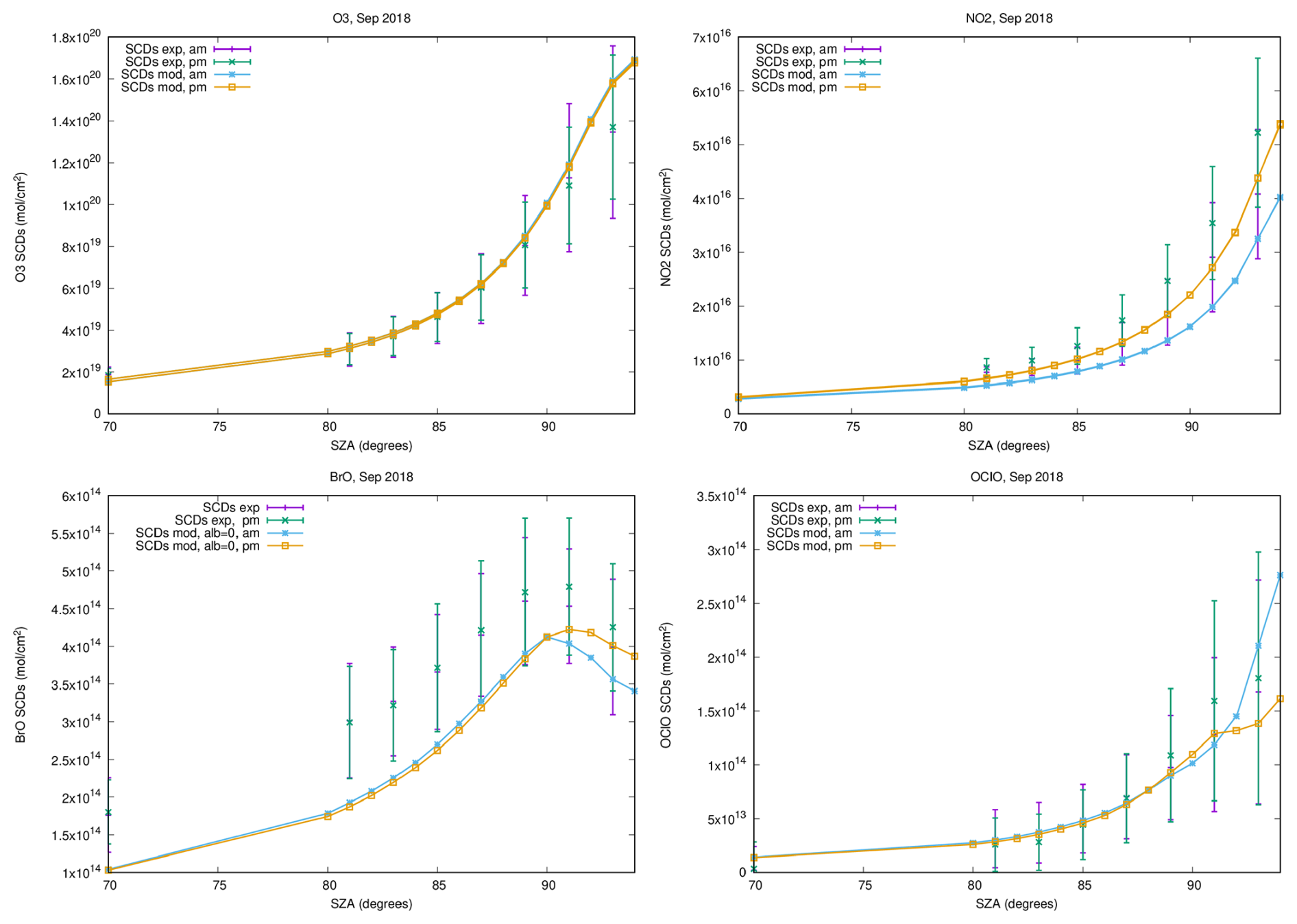
Figure 14 Solar zenith angle evolution of the monthly SCDs of O₃ (top left), NO₂ (top right), BrO (bottom left) and OClO (bottom right) over Marambio during September 2018. Violet and green lines are measured values (am and pm, respectively). Blue and yellow lines are modelled values (am and pm, respectively).

All year round, measured O₃ SCDs are very well captured by mean and std modelled values (less than 7.7 % difference), which give us confidence in the methodology used in this work. Regarding NO₂, measured and modelled SCDs agree within the one sigma std of the measurements accumulated in 10 d periods. Regarding BrO, modelled SCDs are smaller than observations, particularly for winter, with a maximum relative difference of ∼20 %. Similar differences can be seen for mean measured-modelled OClO, although in this case values fall within the one sigma variability of the measurements. Regarding BrO, frequent tropospheric bromine explosions have been reported at Marambio (Prados-Roman et al., 2025), which could lead to a contamination of the observed SCD by tropospheric BrO even at high SZA.

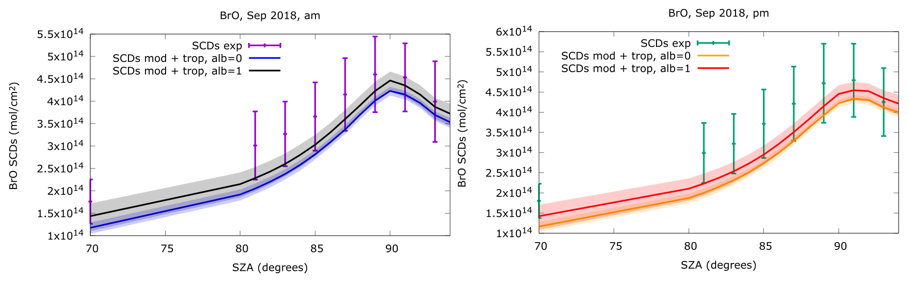
Figure 15 Solar zenith angle evolution of the monthly SCDs BrO over Marambio during September 2018. Violet and green lines are measured values (am and pm, respectively). Left panel: Blue and black lines are am modelled values (surface albedo =0 and =1, respectively). To take into account possible tropospheric BrO explosions, these simulated SCD values consider a tropospheric BrO contribution representative of the BrO values observed at Marambio during September (6.5×10¹² molec. cm⁻² in the first 2 km, Prados-Roman et al., 2025). Shaded aeras correspond to minimum (no tropospheric BrO) and maximum (12.0×10¹² molec. cm⁻² in the first 2 km, Prados-Roman et al., 2025) tropospheric values observed at Marambio during September. Right panel: Orange and red lines are pm modelled values (surface albedo =0 and =1, respectively). Shaded areas correspond to the same minimum and maximum tropospheric values as the left panel.

In Fig. 14, the evolution of the measured SCDs with the SZA (violet for am and green for pm) and the corresponding modelled values (yellow for am and blue for pm) have been represented for Marambio in September. In addition, to consider the possible impact of tropospheric BrO, SCDs simulated with an added tropospheric contribution representative of what is observed at Marambio at this time of the year (6.5×10¹² molec. cm⁻² in the lower 2 km of the atmosphere Marambio, Prados-Roman et al., 2025), are also plotted in Fig. 15. The left panel of Fig. 15 corresponds to sunrise (am) values and right panel to sunset (pm) values. Blue and orange lines correspond to surface albedo =0 and black and red lines to albedo =1. Shaded areas correspond to the range of values between the maximum tropospheric BrO observed at Marambio during September (12.0×10¹² molec. cm⁻²: median value from 2015 to 2023, Prados-Roman et al., 2025) and minimum (no) BrO. While the surface albedo has a small influence in the “pure” stratospheric SCDs, when considering an extra BrO tropospheric contribution, the role of the albedo becomes more important. As can be seen, when considering this tropospheric BrO contribution, modelled BrO SCDs fall within the error bars (std) of the measured SCDs. This strengthens the hypothesis that tropospheric BrO is the main cause for the observed differences between measured and modelled BrO SCDs shown in Fig. 13.

Additional possible sources of error for all measured SCDs represented in Fig. 13 could be the estimation of the SCD in the reference spectrum. Moreover, we must consider the limited spatial resolution of the SLIMCAT 3-D chemical transport model simulation used (2.8°×2.8°). During active vortex periods, this limited model resolution may complicate the comparison with observations, particularly in Marambio, which is highly affected by the dynamics of the polar volar edge. The photochemical model profiles are used as inputs of AURA and DISORT as if they were representative of the whole atmosphere. In the worst case, for SZA =94°, we are considering regions up to 8° distant from the station. Even if the solar beams arriving at the stations from such distances are the most attenuated, so they contribute less to the modelled quantities, it must be kept in mind that this is also an approximation. A further detailed analysis of the differences found herein is beyond the scope of this work and will be the subject of future studies.

5 Conclusions

Stratospheric AMFs for O₃, NO₂, BrO and OClO at Marambio and Belgrano Antarctic stations have been calculated for the year 2018. They have been obtained by using a spherical Monte-Carlo RTM. Temperature, pressure and optical-path-averaged concentration vertical profiles obtained from a photochemical box-model have been used as input in the RTM. These optical path averages have been calculated considering the trace gas concentrations encountered at the different SZAs during twilight. To our knowledge, BrO and OClO stratospheric AMFs are reported for the first time for SZAs up to 94° taking into account photochemistry and optical path averages of the concentrations.

To simplify the complex calculations, monthly averaged AMFs have been calculated (see values in Supplement). The impact of the temporal sampling in the calculation of these quantities has been studied at Marambio, concluding that for NO₂ and OClO shorter temporal sampling is recommended for this site, especially during the months of June and July. Comparing the obtained O₃ and NO₂ AMFs with those provided by 2D-DISORT, a good agreement is found. However, when comparing with NDACC AMFs, while all datasets show similar results for O₃, larger differences are observed for NO₂. Considering that 2D-DISORT and MYSTIC simulations produce similar results, these differences are attributed to the different concentration profiles used as input in NDACC as compared to the photochemical concentration profiles used in this work.

Our results show that, for the photoactive species considered in this work, the evolution of the AMFs and SCDs with the SZA depends primarily on their photochemical variations (total concentration and its vertical distribution), the optical path followed by the sunlight beams, i.e. the geometry of the problem (observation view, Earth sphericity, Sun position, etc), and the effective scattering altitude.

To validate our results, simulated SCDs of the four considered compounds have been compared to measurements performed in Marambio during 2018. A general good agreement is found for O₃, NO₂ and OClO. Although some discrepancies are found in winter for BrO, they can be attributed (mostly) to the contribution of the tropospheric BrO that is not taken into account in the photochemical profiles, but that have a significant influence on the total BrO SCDs even for zenith measurements. In that case (of large tropospheric contribution), surface albedo also significantly influences the results. In general, for all four species, a good agreement is found within one sigma standard deviation. Assuming that the photochemical model is accurate; this confirms the validity of the method employed and the approximations considered.

For future work, it would be interesting to study the influence that clouds and/or orography may have on calculations, as well as the influence of stratospheric dynamics.