The added value of new ground-based observations in improving China's methane emission quantification

China is one of the largest anthropogenic methane emitters, yet its current space- and ground-based observational network remains insufficient for robust emission quantification, particularly in southern regions. To address this gap, we develop an integrated framework, employing Bayesian analytical inversion and simulated annealing algorithms, to design optimal ground-based methane monitoring networks. In Bayesian theory, the degrees of freedom for signal (DOFS) is usually used to quantify the number of independent information provided by observations, with higher values indicating stronger constraint capability. Using GEOS-Chem at 50 km resolution, we estimate that current TROPOMI observations and existing surface measurements (13 in situ sites and 4 ground column sites in East Asia) can provide a DOFS of 134 for methane emissions in China. We further assess the performance of networks comprising 5 to 100 new stations across daily, weekly and monthly sampling frequencies. Optimized designs consistently prioritize new sites in southwestern and eastern China, where satellite coverage is sparse and emissions are high. Adding 50 optimally placed stations with weekly sampling can approximately double the DOFS (from 134 to 259). These results highlight the significant potential of combining optimized ground-based networks with satellite data to improve methane emission quantification in China.

1 Introduction

Methane is the second most important greenhouse gas, contributing approximately 0.6 °C of global warming since pre-industrial times (Naik et al., 2021). Owing to its relatively short atmospheric lifetime (9.1 ± 0.9 years) (Prather et al., 2012), methane mitigation is widely regarded as one of the most near-term strategies for keeping the 1.5 and 2 °C temperature targets (IPCC, 2023). China is one of the world's largest anthropogenic methane (CH₄) emitters, accounting for nearly 14 % (53 [34–66] Tg a⁻¹ out of 369 [350–391] Tg a⁻¹) of global anthropogenic emissions (Saunois et al., 2025). In November 2023, the Chinese government released its first national methane action plan, which prioritizes enhanced emission monitoring through integrated space- and ground-based observations (Methane Emission Control Action Plan, 2024). However, large discrepancies among existing methane inventories hamper the formulation of effective mitigation targets. Current bottom-up estimates, which rely on emission factors and activity data, differ by at least 30 % for national-scale anthropogenic methane emissions (e.g., 63 Tg a⁻¹ in EDGARv6, Crippa et al., 2026, versus 48 Tg a⁻¹ from Peking University CH₄ version 2 inventory, Liu et al., 2021). These inconsistencies underscore the need for observation-based, or “top-down” approaches to provide independent constraints and reduce uncertainty in methane emission estimates.

Current observations remain insufficient to robustly quantify China's methane budget. This limitation arises primarily from (1) inadequate spatiotemporal coverage of existing satellite observations and (2) sparse surface monitoring stations across China (Wang et al., 2025). Current “top-down” quantification primarily relies on Shortwave Infrared (SWIR) sensors (e.g., TROPOMI, GOSAT) that exhibit sufficient sensitivity to surface methane concentrations, but suffer from frequent data gaps due to cloud cover (particularly in southern China during the monsoon season) and complicated terrains (Southwest, Tibet, Northeast). For example, Zhong et al. (2025) showed that sectoral emission estimates for rice paddies, lakes, and wetlands – predominantly located in southern China – exhibit large posterior uncertainties (53 %–69 %), coinciding with low satellite data availability driven by monsoon-related cloudiness (Tang and Chen, 2006). These limitations underscore the urgent need for complementary ground-based networks to constrain these uncertainties. Despite this recognized need, the optimal design of such monitoring networks remains poorly understood – a key research gap our study aims to address.

While previous studies have optimized monitoring networks to improve CO₂ emission quantification (Kaminski and Rayner, 2017; Nickless et al., 2018, 2020; Park and Kim, 2020; Patra and Maksyutov, 2002; Rayner et al., 1996; Villalobos et al., 2025; Wang et al., 2023), far less attention has been given to designing CH₄ monitoring networks, particularly for China. Although a recent study (Zhang et al., 2023) employed proper orthogonal decomposition to optimize CH₄ monitoring locations in China, it focused on reducing the uncertainties of reconstructed methane concentrations rather than emission fluxes. Accurate emission inversion requires an additional step, which is typically achieved by using methods like Bayesian analytical inversion (Shen et al., 2022), the ensemble Kalman filter (Feng et al., 2023) and the 4D-Var inversion (Zhao et al., 2024) frameworks. Among these, Bayesian analytical inversion directly provides the full posterior error statistics (Nickless et al., 2018; Patra and Maksyutov, 2002; Rayner et al., 1996; Wang et al., 2023), whereas other methods generally yield approximate estimates. Separately, identifying the best-performing network requires an optimization algorithm. Previous studies on CO₂ networks typically use incremental optimization (Nickless et al., 2018, 2020; Patra and Maksyutov, 2002; Wang et al., 2023), genetic algorithms (Nickless et al., 2018), and simulated annealing (Rayner et al., 1996). So far, no study has addressed network optimization through the integration of satellite and ground-based observations to improve methane emission estimates.

This work aims to design an optimal CH₄ monitoring network to improve methane emission quantification across China. Building on existing observational networks (TROPOMI and ground stations), we integrate a Bayesian inversion framework, the GEOS-Chem chemical transport model, and the simulated annealing algorithm to maximize observational constraints through strategic placements of new ground stations. Our approach evaluates network configurations of 5–100 new stations at multiple temporal resolutions (daily, weekly and monthly). This Bayesian inverse modeling approach is adapted from our previous work (Zhong et al., 2025). That study demonstrated that while TROPOMI observations can effectively constrain China's total methane emissions, estimating individual sources remains challenging due to its insufficient spatiotemporal coverage. As China expands its CH₄ monitoring network, this work can inform the strategic placement of future stations to better support climate change mitigation efforts.

2 Data and methods

2.1 TROPOMI observations

The Tropospheric Monitoring Instrument (TROPOMI) aboard ESA's Sentinel-5 Precursor (S5-P) satellite provides a global coverage within a day. It retrieves the column-averaged dry-air methane mole fraction (XCH₄) for clear-sky scenes with a spatial resolution of up to 7 km × 7 km at nadir (5.5 km × 7 km since August 2019). We employ the blended TROPOMI+GOSAT product, which applies a machine learning model to correct biases between TROPOMI and GOSAT data (Balasus et al., 2023). To ensure data quality, we only use high-quality retrievals based on previous recommendations (Shen et al., 2022): (1) qa_value ≥ 0.5, (2) blended albedo ≤ 0.85, (3) surface albedo ≥ 0.05, (4) XCH₄ ≤ 3000 ppb, and (5) surface altitudes ≤ 2 km. Due to computational constraints, we limit our analysis to 2022 and rely on satellite observations available for that year.

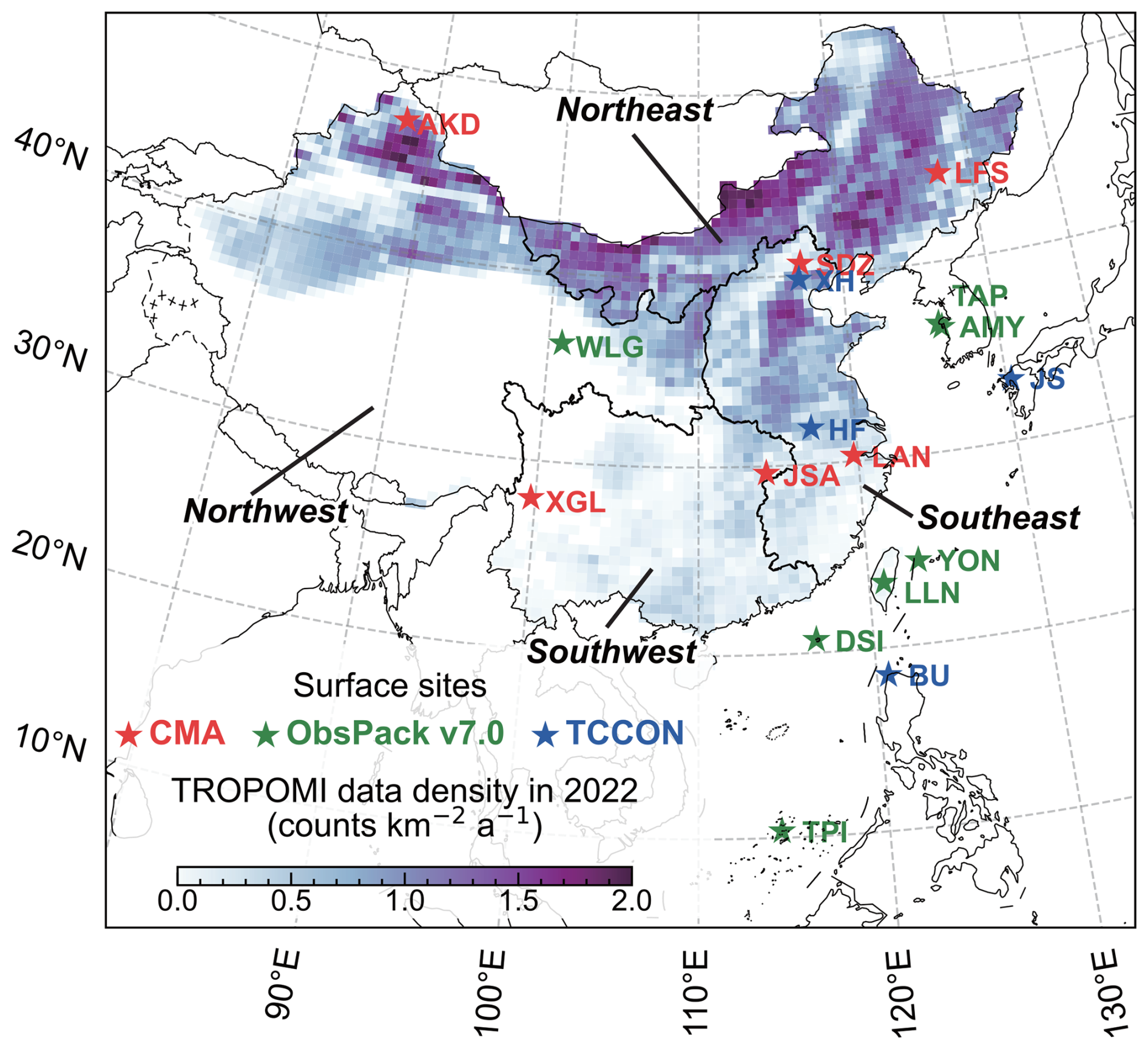
Figure 1 Spatial distribution of TROPOMI methane observation density ($\mathrm{counts}{\mathrm{km}}^{-\mathrm{2}}{\mathrm{a}}^{-\mathrm{1}}$) and ground-based monitoring stations for the year 2022. The surface stations are sourced from networks and databases including the China Meteorological Administration (CMA) (Fang et al., 2013; Wang et al., 2020; Zhang et al., 2022), NOAA GLOBALVIEWplus CH₄ ObsPack v7.0 (Schuldt et al., 2024) and the Total Carbon Column Observing Network (Laughner et al., 2024; Liu et al., 2026; Morino et al., 2026; Shiomi et al., 2026; TCCON Team, 2022; Wunch et al., 2011; Zhou et al., 2026). The TROPOMI observation density is shown at 0.5° × 0.625° horizontal resolution. Additional details regarding the surface site characteristics and TROPOMI observation information are provided in Table 1. The four regions (Northeast, Northwest, Southeast and Southwest) are spatially defined in Fig. 1. TROPOMI data © ESA/Copernicus. GLOBALVIEWplus CH₄ ObsPack data © NOAA. TCCON data © TCCON Team and contributing institutions. Surface station data © China Meteorological Administration (CMA).

After quality control and spatial regridding, approximately 3.8 × 10⁶ valid individual XCH₄ retrievals were obtained over China in 2022 (Fig. 1). It should be noted that regridding performed here is solely for visualization purposes; in the inversion system, each satellite retrieval is assimilated independently, as in previous studies (Shen et al., 2022; Zhong et al., 2025). Data density is highest in northern China, reaching up to ∼ 2.0 $\mathrm{counts}{\mathrm{km}}^{-\mathrm{2}}{\mathrm{a}}^{-\mathrm{1}}$ across Northeast China, Inner Mongolia, Xinjiang, and parts of the North China Plain (NCP). In contrast, retrieval coverage is sparse in southern China, primarily due to persistent cloud cover. Complex terrain further degrades data quality in mountainous regions, where a large fraction of observations is discarded during filtering. As a result, regions south of 33° N account for only 3.8 × 10⁵ valid retrievals – about 11 % of those available in northern China – highlighting a pronounced north–south observational imbalance. This pronounced observational gap in southern China suggests that strategic placement of new ground-based stations in this region may be essential to compensate for the limited satellite constraints.

Table 1 The information of ground-based and satellite observations used in this study.

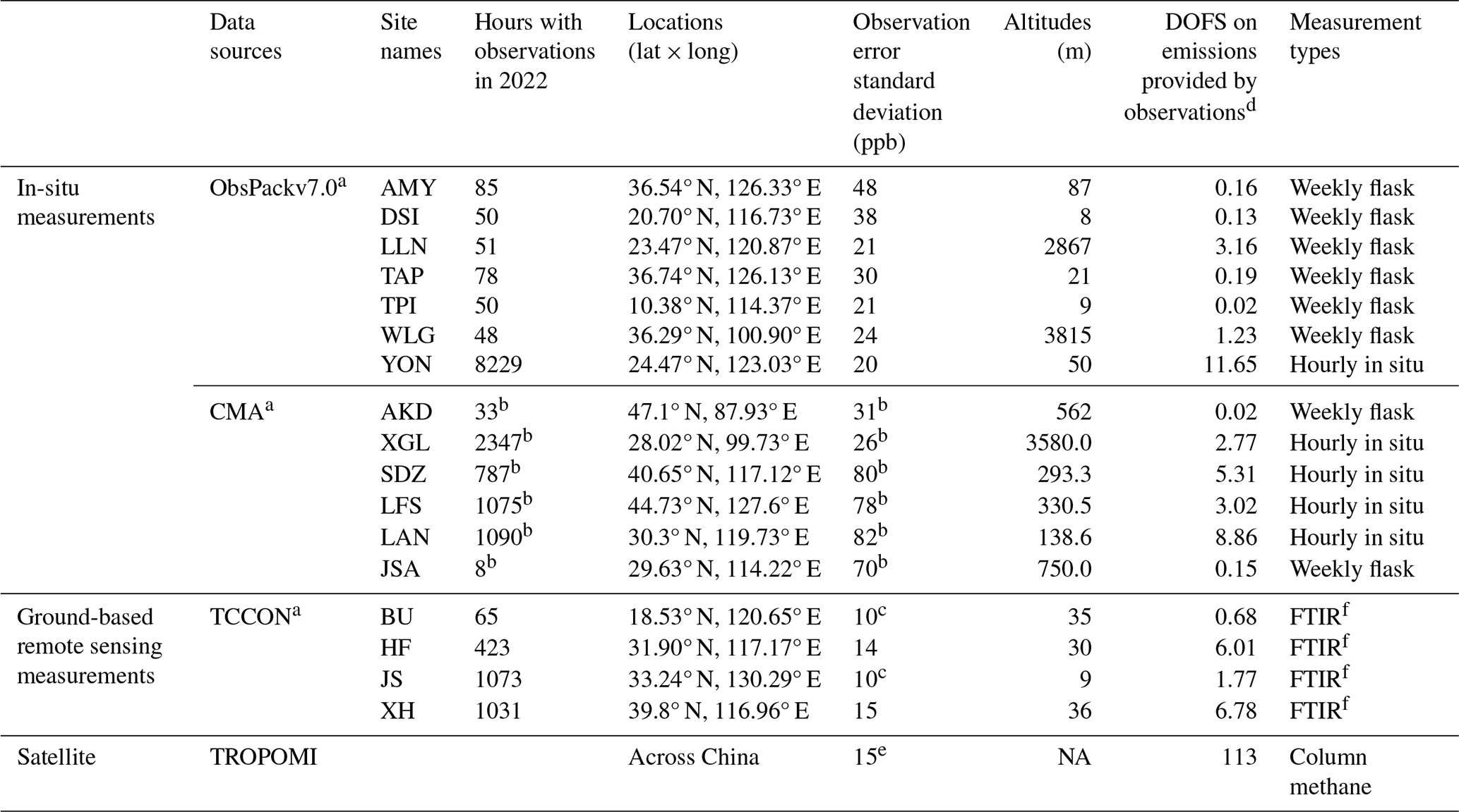
^a The surface observation stations are sourced from the China Meteorological Administration (CMA) (Fang et al., 2013; Wang et al., 2020; Zhang et al., 2022), NOAA GLOBALVIWEplus CH₄ ObsPack v7.0 (Schuldt et al., 2024) and the Total Carbon Column Observing Network (Laughner et al., 2024; Liu et al., 2026; Morino et al., 2026; Shiomi et al., 2026; TCCON Team, 2022; Wunch et al., 2011; Zhou et al., 2026). ^b We assume that the number of observations and the error standard deviation for CMA remain consistent with those from earlier years, as sourced from a previous study (Zhang et al., 2022). ^c The minimum observational error deviation in this study is 10 ppb. ^d Here, we quantify the individual contribution of each individual station and TROPOMI to constraining methane emissions over China, with each observation source evaluated independently. ^e This value represents the average observational error standard deviation (1σ) of TROPOMI retrievals within the grid cell. ^f Hourly Fourier Transform Infrared spectroscopy (FTIR) total column measurements. NA: not available.

2.2 Ground-based observations

This study uses ground-based methane observations from 17 stations across East Asia for the year 2022 (details in Table 1, spatial patterns in Fig. 1), comprising two types of measurements: (1) total column observations and (2) surface-air in situ measurements. The total column data are obtained from the Total Carbon Column Observing Network (Laughner et al., 2024; Liu et al., 2026; Morino et al., 2026; Shiomi et al., 2026; TCCON Team, 2022; Wunch et al., 2011; Zhou et al., 2026), which employs Fourier-transform spectrometers to provide reference abundances of numerous atmospheric species. Among the four TCCON stations in East Asia, two are located in China (Hefei and Xianghe; Fig. 1). For the TCCON data, we only use measurements with solar zenith angles < 60° to ensure high data quality, following a previous study (Liang et al., 2023). Hourly averages are then computed from these measurements.

The surface-air in situ measurements include China Meteorological Administration (CMA) methane monitoring data (Fang et al., 2013; Wang et al., 2020; Zhang et al., 2022) and GLOBALVIEWplus CH₄ ObsPack v7.0 data (Schuldt et al., 2024). For the CMA stations, we note that recent data are not publicly available. Therefore, we apply the observation error standard deviations derived from the documented period of 2010–2017 (Zhang et al., 2022) to our 2022 analysis. This approach is valid because our Bayesian framework, for the task at hand, requires not the actual measured CH₄ concentrations but rather the observation error standard deviation directly computed from residual errors for each surface station and model grid cell (Heald et al., 2004; Rodgers, 2000). For the ObsPack v7.0 dataset, we select East Asian stations (latitude 11° S–55° N, longitude 60–150° E) that recorded methane data during 2022 and remained active thereafter. Spatially, CMA sites are concentrated in densely populated regions of eastern China, whereas most ObsPack stations are located in more remote and sparsely populated areas, providing complementary observational constraints.

2.3 GEOS-Chem chemical transport model and prior emissions

We use the GEOS-Chem chemical transport model (v14.1.0) (Yantosca et al., 2023) to simulate atmospheric methane distributions. The model is driven by MERRA-2 reanalysis meteorological fields from the NASA Global Modeling and Assimilation Office (Gelaro et al., 2017). We conduct GEOS-Chem model simulations at a 0.5° × 0.625° resolution covering East Asia (4–58° N, 64–140° E). Emissions for energy sectors (coal, oil and gas) are from the Global Fuel Exploitation Inventory version 2.0 (GFEIv2) (Scarpelli et al., 2022). Other anthropogenic methane emissions are from the Emission Database for Global Atmospheric Research (EDGARv6) inventory (Crippa et al., 2026), termite methane emissions are from Fung et al. (1991), and aquatic system methane emissions are from Johnson et al. (Johnson et al., 2022). Natural wetland methane emissions are the mean of 18 members of the WetCHARTs v1.3.1 inventory ensemble (Ma et al., 2021).

Figure 2 shows the spatial distribution of the total prior methane emissions in China. Hotspot emissions are concentrated in eastern and southwestern regions, particularly in major coal-producing provinces (e.g., Shanxi and Guizhou) and large metropolitan areas where landfills and wastewater treatment dominate. Based on these bottom-up inventories, total methane emissions in China amount to 68 Tg a⁻¹, with 64 Tg a⁻¹ emitted by anthropogenic sources. Sectoral contributions are estimated as follows: coal mining 21.0 Tg a⁻¹, oil and gas 1.2 Tg a⁻¹, livestock 8.2 Tg a⁻¹, wastewater 9.5 Tg a⁻¹, landfills 5.2 Tg a⁻¹, rice paddies 13.7 Tg a⁻¹, wetlands 2.0 Tg a⁻¹, and lakes and aquaculture 1.3 Tg a⁻¹ (Fig. S1 in the Supplement).

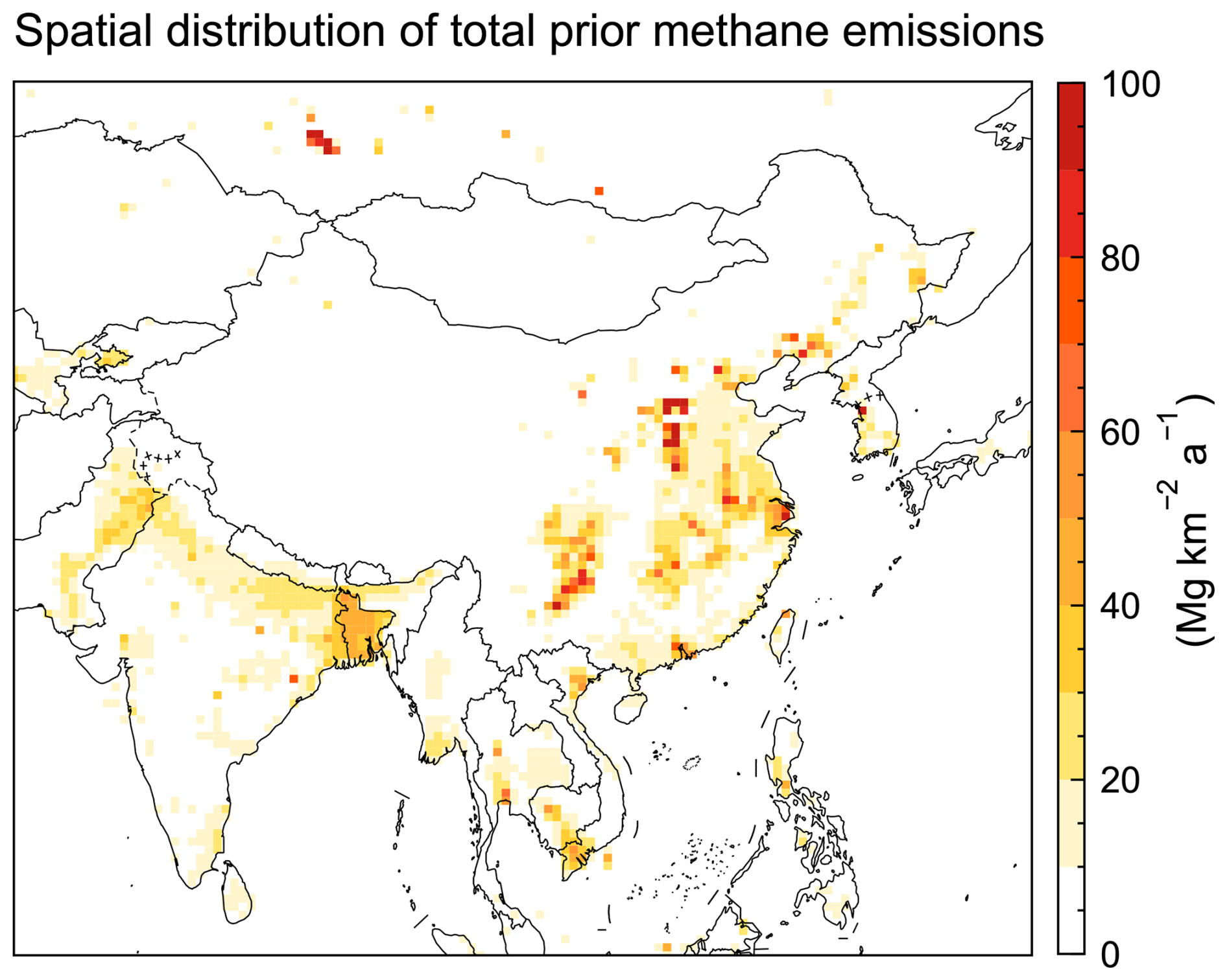
Figure 2 Spatial distribution of total prior methane emissions. See Methods for details about each prior inventory.

2.4 Bayesian analytical inversion

The posterior estimate ($\widehat{\mathit{x}}$) is obtained by minimizing a Bayesian cost function J(x), which assumes normal errors and is regularized by the prior estimate x_A.

$$\begin{array}{}\text{(1)}& \begin{array}{rl}J\left(\mathit{x}\right)=& (\mathit{x}-{\mathit{x}}_{\mathrm{A}}{)}^{\mathrm{T}}{\mathbf{S}}_{\mathrm{A}}^{-\mathrm{1}}(\mathit{x}-{\mathit{x}}_{\mathrm{A}})\\ & +\mathit{\gamma }(\mathit{y}-F(\mathit{x}\left){)}^{\mathrm{T}}{\mathbf{S}}_{\mathrm{O}}^{-\mathrm{1}}\right(\mathit{y}-F\left(\mathit{x}\right))\end{array}\end{array}$$

Our analysis preserves the native spatial resolution of high-emission grid cells (> 1 Gg a⁻¹), while low-emission grid cells (below 1 Gg a⁻¹) are aggregated via K-means clustering to reduce computational cost. This clustering makes use of each gridcell's latitudes, longitudes and 10 sectoral emissions (see Table S1 in the Supplement). Thus, the state vector (x) to be optimized in the inversions comprises 1340 native grid cells at 0.5° × 0.625° resolution, 1834 emission clusters created by the K-means algorithm and 4 elements representing boundary conditions, thus with a total length of 3178 (3178 = 1340 + 1834 + 4). This strategy enables optimization at native resolution for major point and regional sources – primarily in eastern China – while substantially reducing the computational burden associated with sensitivity calculations for diffuse, low-emission regions, which are mainly located in western China and outside the national domain. Note that for all inversions, we only solve for the annual mean correction ratios of the state vector. The relationship between the state vector of methane emissions (x) and GEOS-Chem concentrations (y=F(x)) is assumed to be linear and is expressed as $F\left(\mathit{x}\right)=\mathbf{K}\mathit{x}+c$, where $\mathbf{K}=\partial \mathit{y}/\partial \mathit{x}$ is the Jacobian matrix and c is a constant. This assumption allows us to to explicitly construct the Jacobian matrix using GEOS-Chem simulations. Specifically, we perturb each emission element by 50 % of its prior emission and each boundary condition by +5 ppb. After running the simulations over the inversion period, we compute the resulting concentration changes, which are then used to construct K.

We assume diagonal structures for the prior (S_A) and observational (S_O) error covariance matrices, a choice that offers significant computational advantages but also entails limitations regarding error characterization. On the one hand, this simplification allows us to evaluate the cost function by processing each individual observation independently, thereby avoiding the construction and inversion of a high-dimensional S_O. On the other hand, we acknowledge that a diagonal S_O may not fully account for potential spatial correlations in observation and model transport errors. This assumption can lead to overfitting, particularly when the number of observations far exceeds the number of state vector elements. To address these issues, previous studies have typically employed the parameterization of off-diagonal elements in S_O to represent spatiotemporal correlations (Liang et al., 2023; Zhang et al., 2022) or the super-observation method to aggregate dense retrievals (Chen et al., 2023; East et al., 2025; Pendergrass et al., 2025). However, these techniques cannot fully eliminate the correlation between observations. To prevent overfitting, a regularization factor (γ) is commonly applied to scale the observational covariance matrix (Brasseur and Jacob, 2017). This factor can be determined by (i) the graph-based L-curve method (Hansen, 2000) or (ii) aligning the posterior state cost function with its theoretical expectation (Lu et al., 2021). Following the latter approach, we use γ = 0.02 for TROPOMI observations. This value is the intermediate one from our tests of 0.01, 0.02 and 0.05, as reported in our previous work (Zhong et al., 2025). In contrast, for sparse ground-based observations, we assume uncorrelated observational errors and adopt a γ value of 1 following previous studies (Lu et al., 2021; Zhang et al., 2022).

For S_A, we assume a relative standard deviation of 50 % for each emission element. For S_O, we calculate the observational error standard deviations (σ_O) using the residual error method (Heald et al., 2004). The residual error (ε_O) is defined as the difference between observations (y) and GEOS-Chem prior simulations (y_a), after removing the mean model bias ($\stackrel{\mathrm{‾}}{\mathit{y}-{\mathit{y}}_{\mathrm{a}}}$), as expressed in Eq. (2). The standard deviation of ε_O then gives σ_O (see Table 1).

$$\begin{array}{}\text{(2)}& {\mathit{\epsilon }}_{\mathrm{O}}=\mathit{y}-{\mathit{y}}_{\mathrm{a}}-\stackrel{\mathrm{‾}}{\mathit{y}-{\mathit{y}}_{\mathrm{a}}}\end{array}$$

where y_a is the GEOS-Chem simulation using prior emissions, provided as native 47-layer vertical profiles methane mixing ratio. The observation vector (y) includes data from TROPOMI and ground stations (see Sect. 2.1 and 2.2 for details). Specifically, the inversion assimilates each valid TROPOMI retrieval individually rather than using gridded averages (e.g. super-observations). To generate XCH₄ for comparison with TROPOMI and TCCON total column observations, we apply their respective averaging kernels and prior profiles to the simulations. This transforms the model's vertical distribution into a representative total column. For surface in situ observations, we extract methane dry air mixing ratios from the surface layer of GEOS-Chem for comparison.

In part of the analysis, to account for the potential dependence of observational error on methane concentrations, we calculate the relative residual standard deviation (RRSD) as the standard deviation of the residual error (σ_O) divided by the modelled annual mean methane concentration in each grid cell. We adopt a reference RRSD of 3.3 %, derived from six existing urban sites (Fig. S2). Thus, the hourly observational error (ε_O,i) is calculated as:

$$\begin{array}{}\text{(3)}& {\mathit{\epsilon }}_{\mathrm{O},i}=\text{RRSD}\times y_{\mathrm{a},i}\end{array}$$

where y_a,i is the modeled methane concentration at hour i.

2.5 Error statistics of the Bayesian inversion and quantification of the constraint capability

A key advantage of analytical inversion can provide complete posterior error statistics including the posterior error covariance ($\widehat{\mathbf{S}}$) and the averaging kernel matrix (A):

$$\begin{array}{}\text{(4)}& {\displaystyle }& {\displaystyle }\widehat{\mathbf{S}}={\left(\mathit{\gamma }{\mathbf{K}}^{\mathrm{T}}{\mathbf{S}}_{\mathrm{O}}^{-\mathrm{1}}\mathbf{K}+{\mathbf{S}}_{\mathrm{A}}^{-\mathrm{1}}\right)}^{-\mathrm{1}}\text{(5)}& {\displaystyle }& {\displaystyle }\mathbf{A}={\displaystyle \frac{\partial \widehat{\mathit{x}}}{\partial \mathit{x}}}=\mathbf{I}-\widehat{\mathbf{S}}{\mathbf{S}}_{\mathrm{A}}^{-\mathrm{1}}\end{array}$$

where I is the identity matrix. The posterior error covariance $\widehat{\mathbf{S}}$ quantifies the remaining uncertainty after incorporating observational constraints. The averaging kernel matrix A characterizes the sensitivity of the optimized (posterior) state vector $\widehat{\mathit{x}}$ to the true state x. The diagonal elements of A (ranging from 0 to 1, with 1 indicating full constraint and 0 indicating no constraint) quantify how well the inversion recovers the true value for each state vector element.

The sum of these sensitivities, known as the degrees of freedom for signal (DOFS), quantifies the total number of independent pieces of information provided by the observations (Rodgers, 2000), which can be derived as:

$$\begin{array}{}\text{(6)}& \text{DOFS}=\text{tr}\left(\mathbf{A}\right)\end{array}$$

Thus, DOFS objectively measures the resolving power of an observing system and indicates how much the posterior uncertainty is reduced relative to the prior. A DOFS close to the total number of parameters (e.g. the length of the state vector 3178 in our case) indicates the observations strongly resolve the entire state vector, while a low DOFS implies the solution remains largely dependent on the prior estimate.

However, DOFS do not fully capture the reduction in posterior uncertainty, particularly when systematic or correlated errors are involved. Another useful metric is the information content, which is defined in terms of the Shannon entropy of probability density functions and conceptually linked to thermodynamic entropy (Rodgers, 2000). The information gain (ΔH) of a measurement when the prior error covariance is S_A and the posterior error covariance is $\widehat{S}$ can be written in bits as:

$$\begin{array}{}\text{(7)}& \mathrm{\Delta }H={\displaystyle \frac{\mathrm{1}}{\mathrm{2}}}\left({\text{log}}_{\mathrm{2}}\mathrm{|}{\mathbf{S}}_{\mathrm{A}}\mathrm{|}-{\text{log}}_{\mathrm{2}}\mathrm{|}\widehat{\mathbf{S}}\mathrm{|}\right)\end{array}$$

In this study, we primarily rely on DOFS to characterize information content, while ΔH is computed as a supplementary metric to account for posterior error reduction not captured by DOFS alone.

Following previous studies (Chen et al., 2022; East et al., 2025; Hancock et al., 2025; Nesser et al., 2024), we also quantify the averaging kernel sensitivities of individual source sectors in China by constructing a summation matrix W as follows:

$$\begin{array}{}\text{(8)}& {\displaystyle }& {\displaystyle }{\widehat{\mathit{x}}}_{\text{red}}=\mathbf{W}\widehat{\mathit{x}}\text{(9)}& {\displaystyle }& {\displaystyle }{\mathbf{A}}_{\text{red}}={\mathbf{WAW}}^{\ast }\end{array}$$

The summation matrix W represents a linear transformation that maps the posterior total emissions of the full state vector ($\widehat{\mathit{x}}$) to the reduced state vector (posterior sector-level emissions in China, ${\widehat{\mathit{x}}}_{\text{red}}$), where W is obtained by column-wise normalization of W_nW_cs. Here, W_n is a (p × n) binary mapping matrix, where the rows correspond to the p native GEOS-Chem grid cells, and the columns correspond to the n independent state-vector elements used in this study. W_cs is a (c ⋅ s × p) matrix, where the rows represent each of the s emission sectors within each of the c countries, and the columns represent the p grid cells. Each element of W_cs contains the prior emission of a given sector-country combination in a given grid cell. W_csW_n thus aggregates the prior emission of each sector-country pair (c ⋅ s) from the native grid cell (p) to the state-vector dimension (n). Each column of this matrix is then normalized by the column sum to obtain W. The Moore–Penrose inverse of W, denoted as ${\mathbf{W}}^{\ast }={\mathbf{W}}^{\mathrm{T}}({\mathbf{WW}}^{\mathrm{T}}{)}^{-\mathrm{1}}$, is subsequently used to construct the reduced averaging kernel matrix (A_red) (Calisesi et al., 2005). Consequently, the diagonal elements of A_red represent the average kernel sensitivity per source sector per country; here we present the results for each major source sector in China.

Because our inversion directly constrains only total methane emissions rather than individual sectors, this method attributes sectoral methane emissions based on their prior fractional contributions within each grid cell. This assumes that this prior sectoral contribution is correct in a given grid cell (Hancock et al., 2025). While the high spatial resolution of our inversion helps mitigate the impact of this assumption compared to coarser resolutions, this approach nevertheless introduces an additional source of uncertainty in the sectoral attribution of the posterior results (Cusworth et al., 2021).

2.6 Definition of objective function for simulated annealing algorithm

Simulated annealing (SA) is a heuristic optimization algorithm designed to find the global minimum (or maximum) of nonconvex optimization problems (Guilmeau et al., 2021). The algorithm mimics physical annealing where a solid is heated near its melting temperature and then gradually cooled to remove lattice defects and achieve a stable crystalline structure (Guilmeau et al., 2021; Kirkpatrick et al., 1983). Here, we seek the optimal solution $s^{\ast }\in \mathbf{S}$ that maximizes the DOFS over China. To align with the conventional minimization framework, we define the cost function c(s) as the negative DOFS:

$$\begin{array}{}\text{(10)}& {\displaystyle }& {\displaystyle }c\left(s\right)=-\text{DOFS}\text{(11)}& {\displaystyle }& {\displaystyle }{s}^{\ast }=\arg \underset{s\in \mathbf{S}}{min}c\left(s\right)\end{array}$$

where s represents the candidate grid cells suitable for site deployments and $\mathbf{S}=\mathit{\{}{s}_{\mathrm{1}},\mathrm{\dots },s_{\mathrm{n}}\mathit{\}}$ denotes all possible solutions. In SA, each candidate solution s and its objective function value c(s) correspond to a state and its energy in the thermodynamic analogy, respectively.

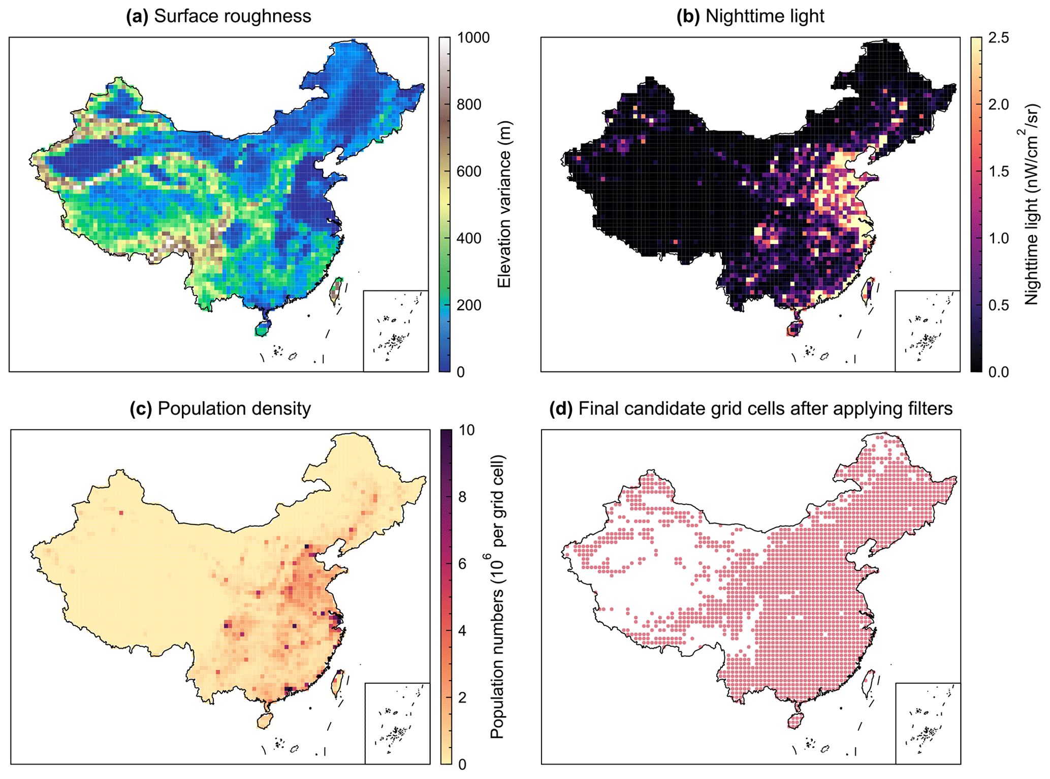
Figure 3 Grid cells suitable for new stations. Panels (a)–(c) illustrate the criteria that determine grid cells suitable for new stations. The following criteria are applied (excluding those containing existing stations): (a) Surface roughness, derived from DEM data (Geospatial Information Authority of Japan, 2025), calculated as the standard deviation of elevation across 30 arcsec pixels within each 0.5° × 0.625° grid cell. (b) Nighttime light intensity from (Elvidge et al., 2013), averaged over 0.5° × 0.625° grids. (c) Population density (Center for International Earth Science Information Network (CIESIN) – Columbia University, 2017). Panel (d) shows the final candidate grid cells after applying all selection filters, where grid cells are excluded if their surface roughness exceeds the 90th percentile, or if either population density or nighttime light intensity falls below the 20th percentile. These filtered grid cells are subsequently used in simulated annealing to identify the optimal locations for new stations. DEM data © Geospatial Information Authority of Japan (GSI). Nighttime lights data © NOAA. Population data © CIESIN, Columbia University.

Before applying SA to optimize station placement, we exclude unsuitable grid cells based on three criteria: (i) the presence of existing monitoring stations within the 0.5° × 0.625° grid cell, (ii) surface roughness (calculated from DEM data (Geospatial Information Authority of Japan, 2025) as the standard deviation of 30 arcsec elevation values within each 0.5° × 0.625° grid cell) exceeding the 90th percentile, and (iii) population density (Center for International Earth Science Information Network (CIESIN) – Columbia University, 2017) or nighttime light intensity (Elvidge et al., 2013) below the 20th percentile (Fig. 3a–c) across the country. These criteria exclude grid cells that are highly mountainous and sparsely populated, where site installation and maintenance are typically costly. Applying these filters yields 2023 candidate grid cells suitable for station placement (Fig. 3d).

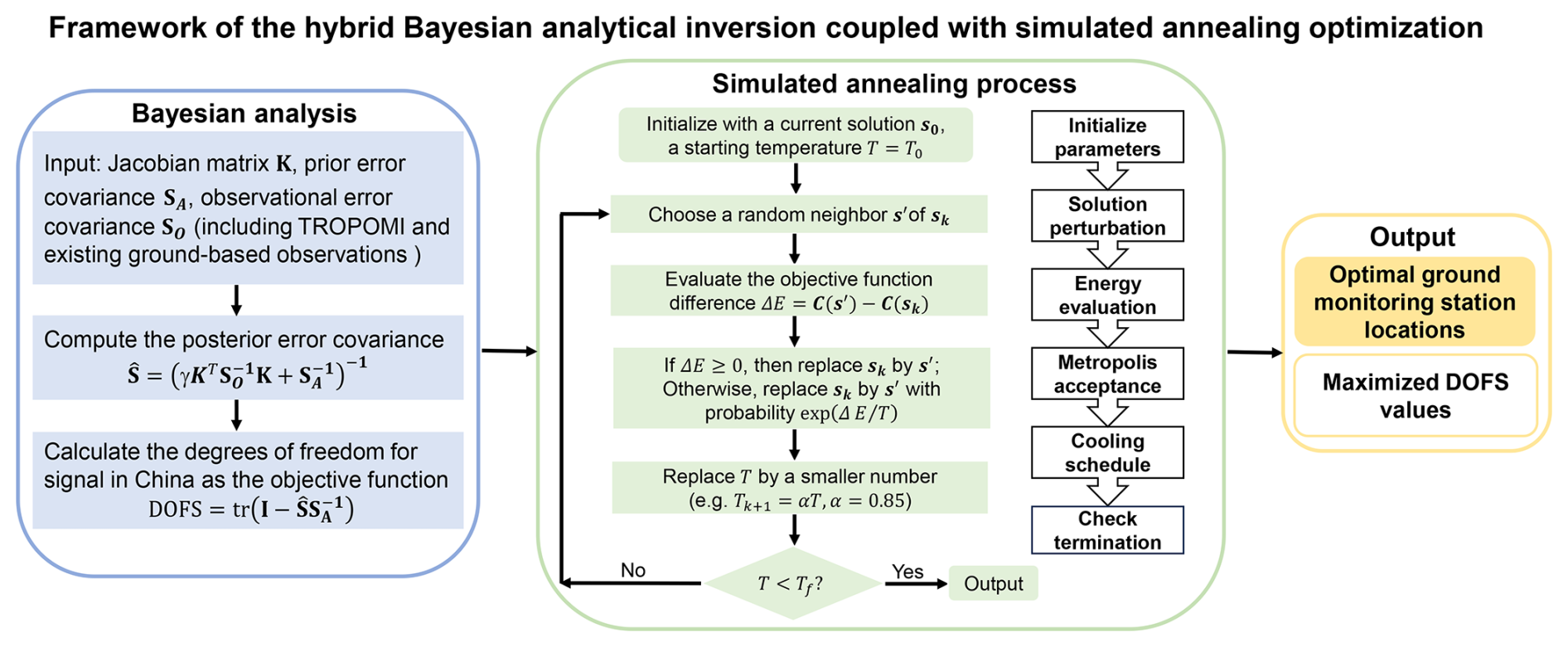
Figure 4 Our framework of the hybrid Bayesian analytical inversion integrated with the simulated annealing algorithm. This workflow integrates satellite and ground-based observations, GEOS-Chem simulations, Bayesian analytical inversion and the simulated annealing algorithm to design the optimal monitoring network. For the simulated annealing process, the left side illustrates the detailed implementation process, while the right side provides a summary of each step.

Four critical parameters must be defined when implementing the SA algorithm: (i) the initial temperature, (ii) the cooling schedule, (iii) the number of trials per temperature, and (iv) the stopping criterion (Souilah, 1995). Following the SA flowchart (Fig. 4), we adopt a geometric cooling schedule (T_k+1 = 0.85T_k) and the number of iterations at each temperature is fixed at 300. The initial temperature is set to T₀ = 1 × 10⁶ and the algorithm terminates when temperature reaches T_f = 1 × 10⁻⁸ after 199 cooling iterations.

2.7 Workflow of the optimization framework

Figure 4 illustrates the workflow of the framework developed in this study to identify optimal locations for a prescribed number of new ground-based observation sites. The approach integrates Bayesian analysis with a simulated-annealing optimization algorithm. The primary objective of this optimization framework is to maximize the total DOFS (a measure of the number of independent pieces of information provided by the observations) of the integrated observing system across China, which accounts for both existing networks and the proposed new sites. Since adding any measurement generally increases DOFS by construction within a Bayesian framework, our optimization focuses on identifying the optimal configurations that provide the maximum information gain.

We evaluate three sampling frequency scenarios for the hypothetical stations: monthly (observation numbersN=13), weekly (N=53), and daily (N=365). In our experimental setup, we assume one representative measurement is taken at the first hour (00:00 UTC, corresponding to 08:00 local time in China) of each day (or the respective week/month) to maintain temporal consistency across the network. While we utilize daily, weekly, or monthly observation data from these hypothetical stations, the state vector of inversion is optimized at an annual resolution. In general, flask-sampling sites typically operate on a weekly schedule within a globally distributed network (Lan et al., 2021); thus, our analysis primarily focuses on results derived from a weekly sampling frequency. For each iteration of the simulated annealing, we begin with a randomly generated set of candidate site locations, s₀, of dimension m (where m ranges from 5 to 100 in this work). The corresponding national total DOFS is then computed using Eqs. (4)–(6). Since s₀ is unlikely to be optimal, we propose a modified configuration by replacing one site in s₀. A proposed change is accepted if it increases the DOFS; otherwise, it may still be accepted with a defined probability to escape local optima. The process is repeated while gradually lowering the “temperature” parameter that controls the rate of energy (here, c(s), negative DOFS) reduction. Iterations continue until all predefined termination criteria are satisfied.

2.8 Evaluation of the performance of the new network

We quantify the benefit of optimizing the network with new stations by calculating the uncertainty reduction (UR) (Park and Kim, 2020; Villalobos et al., 2025).

$$\begin{array}{}\text{(12)}& \text{UR}=\mathrm{100}\times \left[\mathrm{1}-{\displaystyle \frac{{\mathit{\sigma }}_{\text{Posterior}}}{{\mathit{\sigma }}_{\text{Prior}}}}\right]\end{array}$$

where σ_Posterior and σ_Prior denote the 1σ standard deviations of the posterior and prior emission estimations, respectively. Given the stochastic nature of simulated annealing, we perform 50 independent realizations for weekly sampling (and 10 for monthly/daily sampling) for each network size (5–100 stations). To assess the consistency among the resulting optimal network solutions, we conduct pairwise Jaccard similarity analysis (Murphy, 1996) across all realizations. The Jaccard coefficient between two solutions, s₁ and s₂, is defined as:

$$\begin{array}{}\text{(13)}& J(s_{\mathrm{1}},s_{\mathrm{2}})={\displaystyle \frac{\left|s_{\mathrm{1}}\cap s_{\mathrm{2}}\right|}{\left|s_{\mathrm{1}}\cup s_{\mathrm{2}}\right|}}\end{array}$$

It quantifies the overlap between two solutions of selected sites, ranging from 0 (no common sites) to 1 (identical sites).

In summary, our inversion system optimizes a state vector (including native grid cells, clusters and boundary conditions) for the annual mean correction ratios. To evaluate the performance of the newly designed ground-based networks, we employ a multi-scale assessment framework (including DOFS, UR, ΔH and A_red) that spans from individual grid cells to national-level (native grid cells and clusters within China) contributions. First, we define national DOFS as the primary metric and objective function for our simulated annealing algorithm to identify the optimal ground-based network (see Sect. 2.5 and 2.6). Second, we evaluate the enhancement in national DOFS resulting from the addition of a single new site at different locations across China (see Sect. 3.3). Third, based on the optimized networks from the simulated annealing experiments (see Sect. 3.4), we calculate: (i) regional DOFS by aggregating the diagonal elements of the averaging kernel matrix (A) over specific domains (see Sect. 2.5); (ii) grid-scale and regional-scale uncertainty reduction (UR) based on prior and posterior error standard deviations (see Sect. 2.8); and (iii) information gain at the national scale to better capture the overall reduction in uncertainty (see Sect. 2.5). Finally, we derive sector-specific averaging kernel sensitivities (A_red) by employing a summation matrix W to project the high-dimensional A matrix onto sector-specific subspaces and grid-scale (see Sects. 2.5 and 3.5).

3 Results

3.1 Current observation density and error statistics

Current existing observations typically include satellite data and ground-based data. Satellite data coverage is dense in northern and northeastern China, where major coal, livestock, and anthropogenic emissions are concentrated (Fig. S2). In southern China, satellite coverage is sparse due to persistent cloud cover, despite the presence of significant emissions from urban landfills, wastewater and rice paddies. Ground-based stations partially compensate for this gap, including one site in southwest China (XGL) and three sites in central-eastern China (JSA, LAN, HF). Other stations are mainly located in northern China – where satellite density is already high – or in remote, low-emission regions that contribute limited information for quantifying emissions in highly populated or high-emission areas. Consequently, emission estimation remains particularly challenging in southern China (Fig. 1).

Here, we run GEOS-Chem model at the 0.5° × 0.625° resolution, using hourly outputs to estimate observational errors (sum of instrument error, representative error, and forward model error) via the residual error method (Eq. 2). We first compare GEOS-Chem simulated methane concentrations with TCCON and ObsPack v7.0 observations in 2022 (Fig. S3). Pearson correlation coefficients range from 0.57 to 0.88 for TCCON sites and 0.41 to 0.91 for ObsPack sites. The hourly time series show that GEOS-Chem captures temporal variability well, indicating reliable transport representation.

Table 1 summarizes the observation error standard deviations calculated using the residual error method (see Sect. 2.4) for different observation sources (TROPOMI and surface station observations). For ground-based observations representing boundary-layer concentrations (ObsPack and CMA), observation error standard deviations range from 20 to 82 ppb and generally increase from background to urban sites near emission sources. Larger observation errors at urban sites reflect the greater variability in airflow (alternating between polluted and background air) and the difficulty of capturing high-frequency transport features at the model's current resolution. For column-integrated measurements (TCCON and TROPOMI), observation error standard deviations are typically 10–15 ppb. This smaller uncertainty arises because most column methane originates from the free troposphere, where variability is lower, and boundary-layer fluctuations contribute only a small fraction of the total column signal. Based on Table 1, we use the mean observation error standard deviation from six urban sites (TAP, AMY, SDZ, LFS, JSA, and LAN) as a representative estimate for potential new stations (σ_O = 65 ppb). This is because new ground sites are likely to be deployed in eastern China (see Fig. 3d), where emissions are high, so the urban error statistics provide a realistic proxy for expected observational uncertainty in these regions.

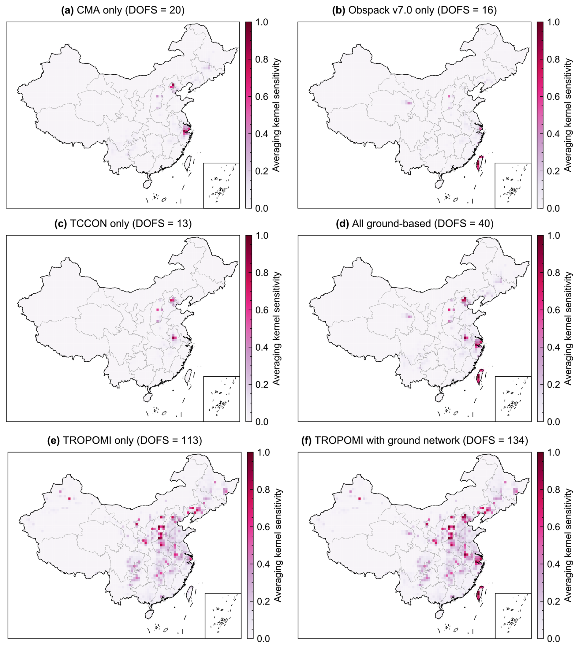
Figure 5 Spatial distributions of averaging kernel sensitivities in China using different observations in the Bayesian inversion. Panels (a)–(d) show observational constraints from (a) CMA (Fang et al., 2013; Wang et al., 2020; Zhang et al., 2022), (b) ObsPack 7.0 (Schuldt et al., 2024), (c) TCCON (Laughner et al., 2024; Liu et al., 2026; Morino et al., 2026; Shiomi et al., 2026; TCCON Team, 2022; Wunch et al., 2011; Zhou et al., 2026), and (d) all ground-based datasets combined. These observational constraints are only based on ground-based measurements and do not include any satellite observations. Panels (e) and (f) show observational constraints from (e) TROPOMI and (f) TROPOMI with all ground-based datasets combined. The DOFS value in each panel title indicates the national total DOFS in China contributed by the corresponding observational network. Surface station data © China Meteorological Administration (CMA). ObsPack data © NOAA. TCCON data © TCCON Team and contributing institutions. TROPOMI data © ESA/Copernicus.

3.2 Current TROPOMI and ground-based observational constraints on methane emissions

Figure 5a–d illustrates the spatial distribution of averaging kernel (AK, Eq. 5) sensitivities derived from the Bayesian inversion based on ground-based methane observations in 2022, excluding satellite data in calculation. These AK sensitivities and associated DOFS values quantify the observational constraints provided by atmospheric concentration measurements on methane emissions. The 17 individual stations, when evaluated independently without synergistic effects from other observations, exhibit DOFS values ranging from 0.02 to 11.65 over China (Table 1). Among all CMA sites, the highest sensitivities occur at SDZ (northern China) and LAN (Yangtze River Delta), both located in high-emission regions. Despite their relatively large observation error standard deviations (80 and 82 ppb), these sites still yield high DOFS values. Theoretically, since the prior error (S_A) and the regularization factor (γ) are kept consistent across all sites, variations in DOFS are primarily driven by the Jacobian matrix (K) and the observation error (S_O). For these two sites, the higher DOFS can be attributed to their stronger local emission fluxes (i.e., higher concentration sensitivity, see Fig. S4) and larger observation numbers, which allow for a greater accumulation of information in the term of the $\mathit{\gamma }{\mathbf{K}}^{\mathrm{T}}{\mathbf{S}}_{\mathrm{O}}^{-\mathrm{1}}\mathbf{K}$ term. Conversely, site such as YON lacks prior emissions within their respective grid cell, but maintains high DOFS values. This is because it can capture transported signals from adjacent sources; furthermore, its high-frequency observations provide robust constraints. The combined DOFS (Eq. 6) for all six CMA sites is 20. In contrast, ObsPack sites – mostly located in remote areas – have substantially lower sensitivity to local emissions, with a total DOFS of 16 across seven sites. The two TCCON sites in China (the other two BU and JS are far away from China), situated in high-emission regions in the North China Plain and Nanjing, contribute a total DOFS of 13, comparable to that of all ObsPack sites. These results indicate that monitoring sites near emission sources provide substantially greater constraints on emissions, and that the current ground network has limited effectiveness for emission quantification and thus requires optimization.

Similarly, we can calculate the total DOFS for satellite observations, excluding ground sites in calculation (Fig. 5e). The TROPOMI-only inversion constrains 113 pieces of information of methane emissions, with stronger AK sensitivities over central and eastern China, a pattern distinct from those obtained from ground sites in Fig. 5d. Weaker constraints are found in southern China due to lower data density as a result of persistent cloud cover, and in western China because of lower methane emission magnitudes (Fig. 2). This spatial pattern of AK sensitivities is consistent with previous findings from GOSAT measurements (Wang et al., 2025). When combined with 17 ground-based observations, the inversion yields a DOFS value of 134 (Fig. 5f), representing an increase of only 19 % relative to the TROPOMI-only case (Fig. 5e).

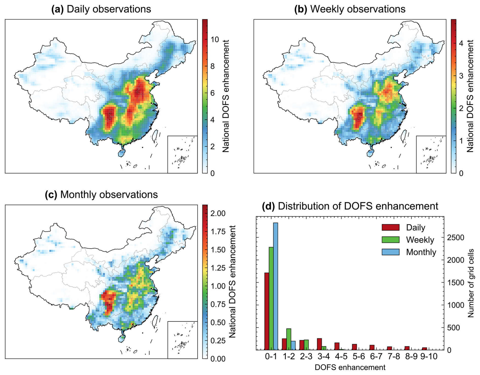
Figure 6 The degrees of freedom for signal (DOFS) enhancement in China by adding one ground station with different temporal frequencies. National total DOFS enhancement from adding one ground station per grid cell on the basis of the existing observational network assuming different sampling frequency: (a) Daily, (b) Weekly, and (c) Monthly. (d) Distribution of DOFS enhancement per grid cell for different sampling frequencies. The x axis represents the DOFS enhancement in each grid cell, divided into 10 evenly spaced bins from 0 to 10. The y axis represents the number of grid cells falling into each bin.

3.3 Added observational constraints from individual new ground sites

We further quantify the potential DOFS improvement by hypothetically adding a single surface station at one grid cell, assuming sampling at monthly (observation numbers N=13), weekly (N=53), and daily (N=365) frequencies (Fig. 6). This assessment builds on the current observing system, which includes TROPOMI and existing ground-based networks (Table 1). For each grid cell, we assume a station is deployed with a prescribed sampling frequency, compute the corresponding Jacobian matrix, and update the national total DOFS. The resulting DOFS increment relative to the current observing system represents the additional constraint provided by a new station at that location.

The results reveal that most significant DOFS enhancements consistently occur in high-emission, observation-sparse regions of eastern and southwestern China. Hotspots of enhancement include eastern Sichuan, northern Guizhou, and the North China Plain, with high gains along the Yangtze River corridor (e.g., Hubei, Henan, Anhui) and parts of Guangdong and Guangxi. These patterns indicate that new ground sites would be most effective if deployed in these regions. Also, the magnitude of these improvements is sensitive to sampling frequency, with maximum DOFS enhancements peaking at 2.1, 4.7, and 11.5 for monthly (N=13), weekly (N=53), and daily (N=365) sampling per station, respectively. In southwestern China, where ground observations are absent and satellite coverage is minimal, DOFS gains are consistently the highest across all sampling frequencies, highlighting an urgent need for new stations in this region. Figure 6d further summarizes the distribution of DOFS enhancement across China for different sampling frequencies. The proportion of grid cells with low DOFS enhancement (< 1) plummets from 94 % (monthly) to 74 % (weekly) and further to 56 % (daily), underscoring the critical role of temporal resolution in increasing the network's effectiveness. Under daily sampling, DOFS enhancements reach 5–10 in some grid cells, demonstrating the high effectiveness of adding ground-based measurements.

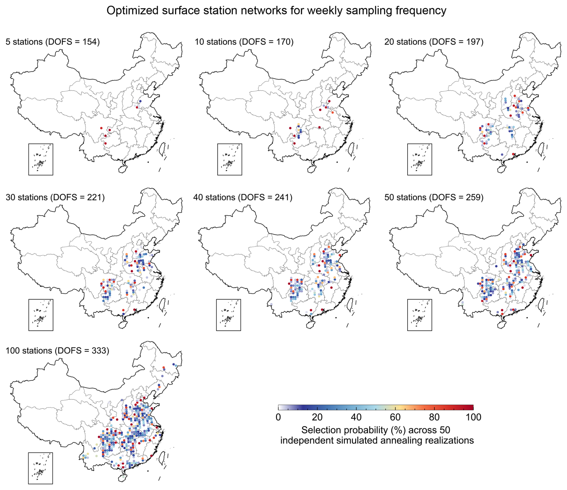
Figure 7 Optimized surface station networks for weekly sampling frequency. The panels show the selection probability (%) of each grid cell for a new site across 50 independent simulated annealing realizations, for network sizes ranging from 5 to 100 new stations. The corresponding increase in the degrees of freedom for signal (DOFS) is displayed within each panel.

Furthermore, to investigate the sensitivity of the observational constraints to the regularization factor and the observation error standard deviation when hypothetically adding a single surface station, we perform additional sensitivity experiments with γ = 0.7 (referencing Zhang et al., 2022) and observation error standard deviations of 75 and 55 ppb (corresponding to 65 ± 10 ppb). As shown in Fig. S5, the spatial distribution of enhancement hotspots remains largely unchanged compared to Fig. 6. Larger σ_O or a smaller γ results in weaker observational constraints.

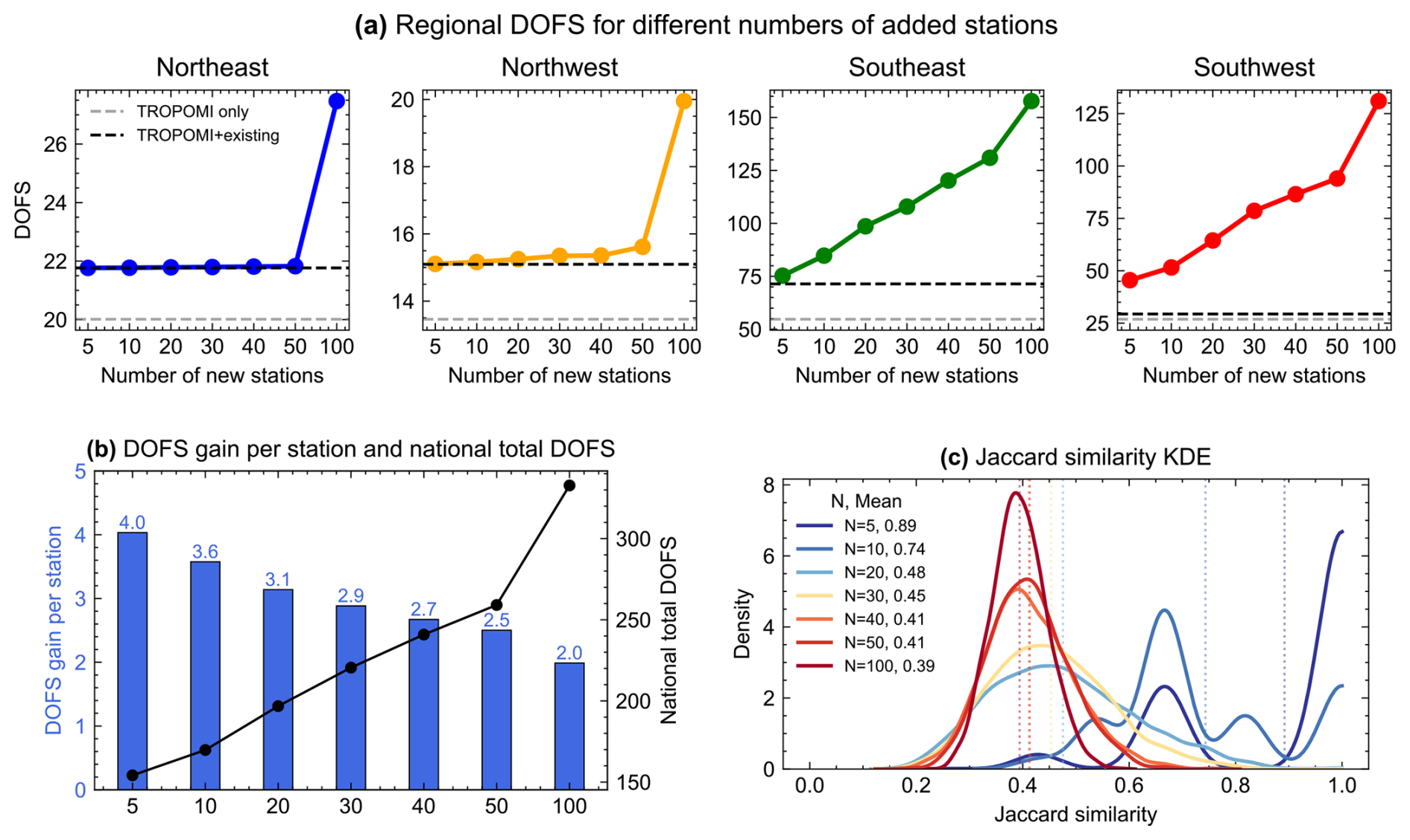
Figure 8 Performance of the simulated annealing algorithm under weekly sampling for different network sizes (5–100 stations) across 50 independent realizations. (a) Regional DOFS in China. Results are shown for four sub-regions (Northeast, Northwest, Southeast, Southwest; see Fig. 1 for regional definitions). (b) Average DOFS enhancement per each newly added station in China, calculated as the DOFS enhancement divided by the number of new sites. (c) Kernel density estimation of pairwise Jaccard similarity across 50 independent simulated annealing realizations. Solid colored curves show the probability density distributions. Vertical dotted lines indicate the mean similarity for each network size (mean values shown in legend).

3.4 Optimal locations for new surface monitoring stations and their posterior error reduction

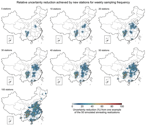
Figure 7 illustrates the optimal locations of surface stations for expanding the ground-based methane networks with 5 to 100 additional surface stations, assuming a weekly sampling frequency. These locations are derived from 50 independent realizations of simulated annealing. For small networks expansions (5–10 stations), new sites cluster primarily in southwestern China and NCP, consistent with the spatial pattern of DOFS enhancements inferred from the single-site sensitivity experiments (Fig. 6). These hotspot regions are characterized by high bottom-up emissions but relatively sparse observational coverage. As the network expands to a medium size (20–50 stations), optimal locations extend southward into Hubei, Hunan, Guangdong, and Guangxi, reflecting persistently low observation density across much of southern China. This spatial clustering directly addresses the critical observing gap previously identified, where the number of valid TROPOMI retrievals in southern China (south of 33° N) is only 11 % of that in northern China. When the network size increases further (e.g., 100 stations), additional sites begin to appear in regions already well covered by satellites (e.g., Northeast China and the Yangtze River Delta) and in lower-emission provinces such as Yunnan, Fujian, and Jiangxi, where the marginal gains in DOFS are comparatively small. Compared to the existing network (DOFS = 134), the optimized networks increase the DOFS by approximately 15 % (DOFS = 154 for 5 stations) and 149 % (DOFS = 333 for 100 stations). Notably, combining the existing network with the newly optimized 50 stations can increase the DOFS to 259, nearly doubling the constraint provided by the existing observation network. We also solve for the optimal locations using the error standard deviations calculated from the RRSD method under a weekly sampling assumption (Fig. S6). The resulting spatial distribution of the newly added stations is largely consistent with that obtained using a fixed standard deviation of 65 ppb.

To examine the spatial heterogeneity of observational constraints, we also calculate the DOFS values for four sub-regions of China (Northeast, Northwest, Southeast, Southwest; regional definitions illustrated in Fig. 1). As shown in Fig. 8a, the gray and black dashed lines represent DOFS values from TROPOMI-only and from TROPOMI combined with existing surface stations, respectively. The current observational network (TROPOMI + ground observations) yields regional DOFS values of 71 in the Southeast, 29 in the Southwest, 22 in the Northeast, and 15 in the Northwest. Notably, existing surface stations result in a significant DOFS improvement in the Southeast (ΔDOFS = 17), while the other three regions show smaller changes (ΔDOFS < 2.5) relative to TROPOMI-only observations. When hypothetical stations are added, the Northwest and Northeast show almost no increase in DOFS relative the baseline for network sizes of 5–50 stations, only with notable gains when the size increases to 100 stations. In contrast, the southern regions benefit substantially from newly deployed sites, with the DOFS increase by 6 %–121 % in the Southeast and by 55 %–345 % in the Southwest as network size grows from 5 to 100 sites.

The national average gains per every new station are shown in Fig. 8b. For example, under the weekly sampling frequency, when 100 new sites are added, the DOFS increases by 199 (from 134 to 333), corresponding to an average gain of 2 DOFS per site. The results exhibit diminishing returns, with DOFS dropping from 4 per site in a 5-station network to 2 in a 100-station network. This behavior indicates that relatively modest network expansions can already deliver substantial improvements; for instance, adding 50 stations yields DOFS gains comparable to those from the entire existing observing system.

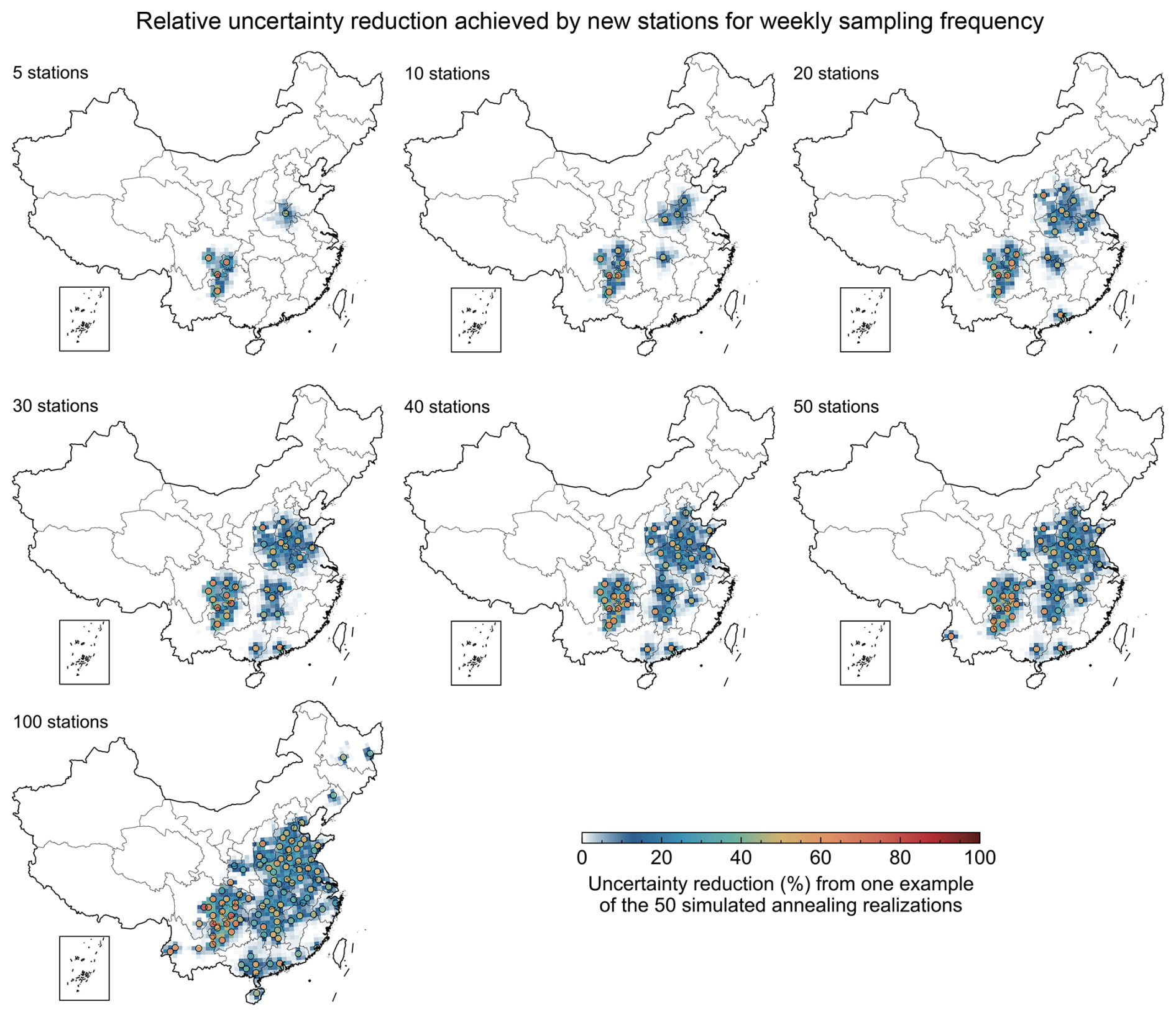
Figure 9 Spatial distribution of the relative uncertainty reduction achieved by expanding the existing observational network under weekly sampling frequency. The figure shows the result from one case of the 50 simulated annealing realizations for different numbers of new stations (ranging from 5 to 100). The existing observational network consists of TROPOMI satellite observations combined with the established ground-based stations. The relative uncertainty reduction (ΔUR) is calculated per 0.5° × 0.625° grid cell. Newly added station locations in each scenario are marked with black circles. TROPOMI data © ESA/Copernicus.

Because simulated annealing is a stochastic optimization method, we also evaluate the consistency of the results using pairwise Jaccard coefficients across 50 independent solutions (Eq. 13). High similarity indicates convergence toward a global optimum, whereas low similarity suggests trapping in local minima. As displayed in Fig. 8c, small networks (N=5, 10) achieve very high mean Jaccard similarity (∼ 0.7–0.9), indicating robust convergence to nearly identical optima, or very likely the global minimum of the objective function. In contrast, larger networks (N≥20) show lower mean Jaccard similarity (∼ 0.4–0.5), reflecting a much larger solution space. For instance, selecting 5 stations from 2023 candidate grid cells yields only 20 000 possibilities, but selecting 100 stations results in an astronomically large number of combinations (approximately 10¹⁷¹). This highlights the increasing complexity of the optimization problem and the greater difficulty in identifying unique optimal solutions as network size grows.

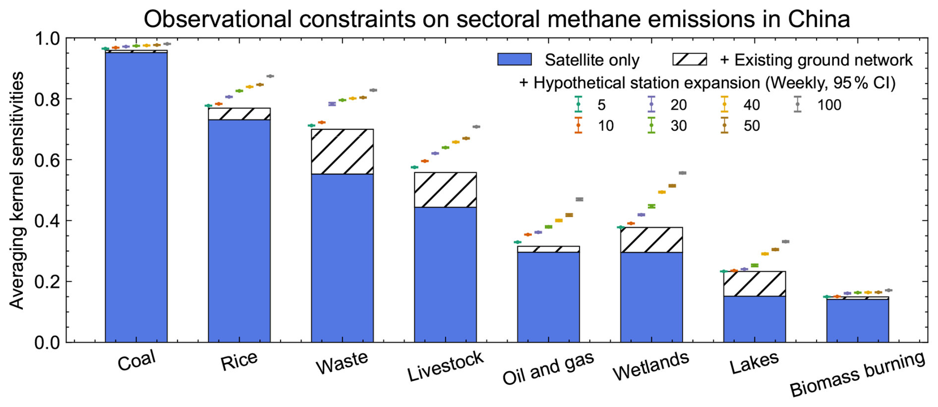
Figure 10 Observational constraint on sectoral methane emissions in China under different observational networks. The blue bars represent AK sensitivities derived from TROPOMI observations alone, while the hatched bars represent the increase in AK sensitivities achieved by incorporating existing ground-based measurements. Colored data points show the mean AK sensitivities after adding new ground stations (weekly sampling frequency), with error bars denoting 95 % confidence intervals from the 50 simulated annealing experiments.

Figure 9 illustrates the relative uncertainty reduction (ΔUR) achieved by a representative case (weekly sampling frequency) selected from 50 independent simulated annealing experiments (as presented in Fig. 7), quantified by comparing posterior uncertainties before and after ground-based network expansion (Eq. 12). The locations of the newly added stations are indicated by the black circles in the figure. As shown in Fig. 9, local relative uncertainty reductions near newly added stations can exceed 50 %–70 %, reflecting the ability of ground-based measurements to directly sample methane enhancements within the boundary layer and to better constrain nearby sources. Such an impact decreases with distance, with uncertainty reductions of 10 %–50 % within 100–200 km and of < 10 % beyond ∼ 200 km. To evaluate the posterior uncertainty reduction at a regional scale, we calculate the regional mean uncertainty reduction (Fig. S7) across the four regions defined in Fig. 1. The posterior uncertainty reduction exhibits significant spatial heterogeneity across regions as the number of added sites increases from 5 to 100. The Southeast and Southwest regions show the most substantial and continuous improvements, with reductions increasing from 9.2 % to 21.3 % and 4.3 % to 13.5 %, respectively. Conversely, the added value in northern regions is much smaller, reflecting the already strong observational constraints provided by the dense coverage of existing TROPOMI data.

In addition to DOFS and UR, we further evaluate the Shannon information gain in bits (Fig. S8). In the Bayesian inversion framework, the information gain quantifies the reduction in the entropy of the state vector from the prior to the posterior distribution. TROPOMI alone provides an information gain of approximately 122 bits, increasing to 156 bits when the existing surface network is included. With the addition of hypothetical stations, the information gain increases monotonically from 193 bits (N=5) to nearly 500 bits (N=100). The marginal increase is largest at the initial stage of network expansion and gradually decreases as more stations are added, reflecting diminishing returns as the newly added observations become increasingly redundant with the existing observational constraints.

To examine how the temporal resolution of observations influences the optimal station network, we conduct similar experiments but using monthly and daily sampling frequencies (Fig. S9). The identified priority regions – southwestern, eastern, and southern China – remain overall consistent across sampling frequencies. Also, the network optimized using daily sampling frequency exhibits a more spatially dispersed pattern. This occurs because the stronger constraint provided by high-frequency measurements at individual sites reduces the need for spatial clustering, allowing the optimization algorithm to prioritize broader geographical coverage over maximal local gains, thus extending sites to regions with lower individual DOFS improvements.

3.5 Observational sensitivity to sectoral emissions from new surface stations

Here we assess the AK sensitivity for each source sector (Eq. 9; see Methods for details). Figure 10 shows the sectoral AK sensitivity derived from different combinations of observations. TROPOMI alone strongly constrain high-emission sources such as coal mining (AK sensitivities = 0.95), providing moderate constraints on rice cultivation (0.73) and waste (0.55), and limited constraints on low-emission sources like lakes, biomass burning, wetlands and oil/gas (0.14–0.30). The addition of existing ground-based observations leads to improvements in the AK sensitivities for key sources like waste and livestock, with increase of +0.15 and +0.11, respectively. However, for other sources, such as oil/gas, wetlands, lakes and biomass burning, observational constraints remain low. The AK sensitivities of these sectors are below 0.5, indicating that their posterior estimates still rely heavily on prior information.

The deployment of new ground stations (at weekly sampling frequency) further enhances observational constraints. Each colored data point in Fig. 10 represents the sectoral AK sensitivity for a specific number of newly added stations, with vertical error bars indicating 95 % confidence intervals from the 50 independent realizations. The degree of improvement varies substantially across sectors. For coal mining and biomass burning, sensitivity improvements are minimal (∼ 0.02) even with 100 new stations. The AK sensitivity of the inversion depends on emission magnitudes and observation density. For coal mining, the minimal improvement in AK when adding new sites is primarily because these large sources are already well-constrained by the current network, with AK values already nearing unity (Fig. 10). For biomass burning, the limited improvement is primarily due to its small emission magnitude (∼ 0.2 Tg a⁻¹). In contrast, sectors such as wetland, oil/gas, livestock, waste, rice, and lakes exhibit much larger sensitivity increases, with maximum AK increments of 0.21, 0.18, 0.16, 0.14, 0.11, and 0.11, respectively, under 100 new stations. After adding 100 stations, the AK sensitivities for most sectors (except lakes and biomass burning) are above 0.5. Figure S10 presents results under monthly and daily sampling frequencies, which broadly align with the weekly-sampling findings. Daily sampling yields markedly stronger constraints, with AK sensitivities for coal, rice, waste and livestock exceeding 0.8. This represents a substantial improvement in posterior emission estimates through optimized ground observation expansion.

4 Discussion and Conclusion

In this study, we systematically evaluate and strategically optimize China's methane monitoring network by integrating TROPOMI observations with ground-based measurements, using a Bayesian inversion framework and the simulated annealing algorithm. The current observational network offers limited spatiotemporal coverage for methane monitoring. Satellite data (TROPOMI) alone provide 113 degrees of freedom for signal (DOFS), while the combination with ground-based observations increases the DOFS to 134 (Fig. 5e and f), which represents a 19 % enhancement. Under weekly sampling, the optimized network increases the DOFS to a range of 154–333, achievable with the addition of 5 to 100 new stations (Fig. 7). Notably, expanding to 50 optimally located stations would nearly double the current system's constraint capability (DOFS from 134 to 259). In addition, optimized designs consistently prioritize new sites in southwestern and eastern China, where satellite coverage is sparse and emissions are high.

While our network optimization framework represents a significant advance in monitoring design, this study is subject to several limitations. These uncertainties primarily stem from inversion assumptions and the limited availability of observational data. First, our framework assumes diagonal observational and prior covariance matrices. This assumption of independent errors is likely unrealistic and can lead to overfitting. We apply a regularization parameter (γ) to avoid overfitting. For ground-based stations, we test two values (0.7 and 1) and obtain consistent results (Sect. 3.3). Second, due to the lack of publicly available CMA recent data, the 2022 analysis relies on error characteristics from earlier years. Since the calculation of DOFS requires only error information rather than actual observations, this approach assumes that the error characteristics constant over time, which may introduce additional uncertainty. Third, the spatial patterns of prior inventories can substantially affect the estimates of DOFS (Chen et al., 2022). This may bias site selection toward regions where prior emissions are potentially overestimated. Furthermore, our current framework does not consider complementary information from other satellite datasets. In particular, thermal infrared (TIR) sensors such as IASI offer distinct vertical sensitivity profiles (Siddans et al., 2017), and China's Gaofen-5B also has the potential to enhance detection capabilities (He et al., 2024). Incorporating these observation platforms would represent meaningful directions for future improvements to the network design strategy.