Operational performance of the Vaisala CL61 ceilometer for atmospheric profiling

The Vaisala CL61 is a new generation elastic backscatter lidar that extends the capabilities of conventional automatic low-power lidars and ceilometers by providing depolarization ratio measurements. Reliable use of these measurements, however, requires thorough evaluation and characterization of the instrument performance and subsequent corrections applied. In this study, performance of multiple CL61 instruments across different sites over 3-year period has been assessed. Results indicate some differences between instruments, with most of these early production units exhibiting a pronounced decrease in laser power over time, accompanied by an increase in background noise likely due to weaker return signals. Normally, the instrument scales the internal calibration factor to compensate for changes in laser power and thus provide consistent attenuated backscatter coefficient values from profile to profile over time. However, for the instrument at the Lindenberg site, by performing manual calibration with atmospheric targets, it is noted that once the laser power dropped below 40 % there is no further compensation in the internal calibration factor.

The instrumental background noise and bias, characterized using the termination hood, are found to vary with temperature. A method has been developed for correcting the instrumental bias and for estimating the associated uncertainty. Additionally, an approach to estimate the uncertainty of volume and particle backscatter and linear depolarization ratio is presented. In a case study representing low aerosol load conditions in Finland, correcting for the instrumental bias changes the volume linear depolarization ratio by up to 0.005 relative to the instrument-provided values. On the other hand, the difference between volume linear depolarization ratio and particle linear depolarization ratio reached up to 0.1. These findings demonstrate that the CL61 firmware effectively removes the majority of the mean background bias, whereas accounting for the molecular contribution is important for quantitative interpretations of aerosol measurements at CL61's wavelength of 910.55 nm. Finally, signal loss in one unit has been traced to fogging of the inside surface of the window, and attributed to insufficient internal heating linked to the instrument's firmware behavior.

1 Introduction

Automatic low-power lidars and ceilometers (ALC) are ground-based elastic backscatter lidars originally developed for the automated detection of cloud base height to support aviation and meteorological operations. Over the past 2 decades, advancements in both hardware and data processing have greatly enhanced their capabilities (Cimini et al., 2020). Notably, improvements in signal quality, particularly in signal-to-noise ratio, now enable ALC to provide profiles of attenuated backscatter coefficient with sufficient dynamic range to permit the observation of a wide range of atmospheric phenomena, including rainfall (e.g. Rocadenbosch et al., 2020; Roschke et al., 2025), fog (e.g. Haeffelin et al., 2016; Ribaud et al., 2021), icing (e.g. Hämäläinen et al., 2020), and even the quantitative estimation of aerosol concentrations (e.g. Shang et al., 2021; Filioglou et al., 2025). ALC data are also increasingly used to estimate atmospheric boundary layer height (e.g. Kotthaus et al., 2023), which is a critical parameter for numerical weather prediction and air quality models (e.g. Uzan et al., 2020; Barragán et al., 2023). Their ability to operate autonomously and reliably in challenging environmental conditions, as well as being eye-safe, makes them well-suited for long-term monitoring and integration into operational networks of national meteorological services and research institutions (e.g. Hirsikko et al., 2014). Many such organizations are actively investigating the use of ALC profile data to improve forecast model performance (e.g. Warren et al., 2018; Illingworth et al., 2019).

Vaisala has recently introduced the CL61 ceilometer, which is an ALC with the capability of measuring the volume linear depolarization ratio δ_v. It is the ratio of the perpendicular to the parallel component of the backscattered signal relative to the emitted polarization. This ratio provides insight into particle sphericity (e.g. Burton et al., 2012; Mamouri and Ansmann, 2016; Baars et al., 2017) and is essential for distinguishing various aerosol types (e.g. Illingworth et al., 2015; Nicolae et al., 2018; Floutsi et al., 2023; Filioglou et al., 2023; Le et al., 2024) such as pollen, smoke, dust, marine, and volcanic ash. It is also utilized in determining cloud phase (Sassen, 1991) and in the retrieval of cloud microphysical properties (Donovan et al., 2015).

To fully leverage the broad range of applications enabled by the CL61, including its new capability to measure δ_v, careful quality control of the backscattered signal from both polarizations is essential. Environmental conditions, such as temperature and relative humidity, can influence lidar performance (Campbell et al., 2002), making it necessary to assess their impact on data quality. For instance, Hervo et al. (2016) identified and corrected a temperature-dependent effect on the overlap function of a Lufft CHM15K ceilometer, which arises from temperature-induced changes in the laser as well as in the instrument's optical and electronic components. Similarly, the older Vaisala CL31 ceilometer has been known to have backscatter artifacts below approximately 70 m (Van der Kamp, 2008; Martucci et al., 2010; Tsaknakis et al., 2011), prompting many studies to omit these near-surface measurements. Identifying and correcting such artifacts in the CL61 would enable reliable observations extending down to heights that overlap with surface-based observations. This capability is especially valuable for studying near-surface meteorological phenomena such as fog, haze, and emissions from ground-level aerosol sources.

In this study, we present a long-term evaluation of the CL61 ceilometers conducted at four different ACTRIS cloud profiling sites in Finland and Germany. Our analysis focuses on the impact of laser power on signal quality, the temperature sensitivity of the instrumental background and methods for its correction. Additionally, we demonstrate our calculation of the uncertainty in the volume and particle linear depolarization ratio (δ_v and δ_p respectively). Finally, we report instances of signal loss attributed to fogging of the inside surface of the window, observed in some of the CL61 units.

2 Instrument description

The CL61 ceilometer, manufactured by Vaisala, is a coaxial ALC system operating at a wavelength of 910.55 nm and equipped with depolarization measurement capability. Its key technical specifications are summarized in Table 1. In brief, the CL61 utilizes an InGaAs diode laser that emits linearly polarized pulses with an energy of 3.9 µJ at a repetition rate of 9.5 kHz. The instrument features a single-lens optical design and performs depolarization measurements using a single-receiver with an avalanche photodiode (APD) detector that switches between two polarizing filters (one perpendicular and one parallel to the polarization of the transmitted pulses) in the same coaxial optical path. The CL61 alternates the acquisition of each polarization every 0.2 s, while using the same receiver module for both channels. Consequently, receiver sensitivity calibration is not required. The maximum detection range of CL61 is 15.4 km.

Table 1 Specifications of the CL61 (CL61 User Guide: https://docs.vaisala.com/r/M212475EN-E/en-US, last access: 21 July 2025).

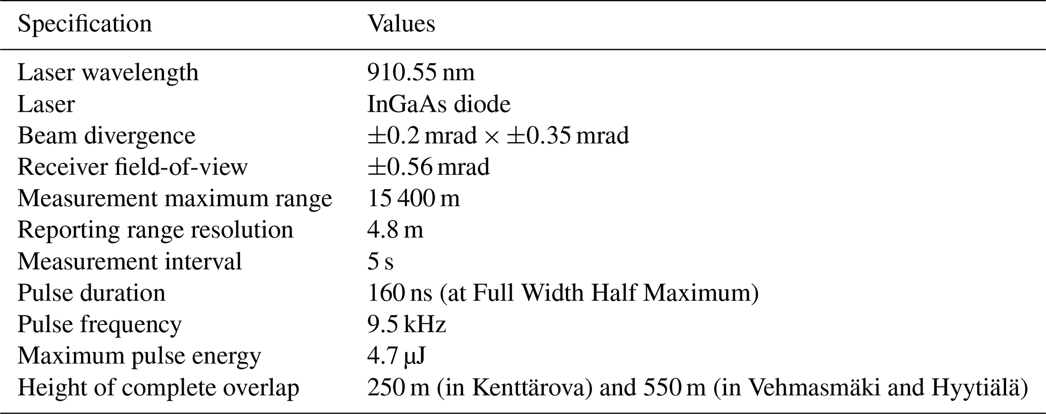
The overlap functions reported by the manufacturer are shown in Fig. S1 in the Supplement. Full overlap between the transmitted laser beam and the receiver field of view is achieved at approximately 250 m range for the instrument at Kenttärova. The instruments at Vehmasmäki and Hyytiälä have different overlap functions, with approximately 95 % overlap at 250 m range and complete overlap at approximately 550 m range. The overlap function is reported only in the new firmware (version 1.2.7), and no overlap function has been reported for the instrument at Lindenberg. Although the overlap function might change during operation, for example due to temperature variations (Hervo et al., 2016), the overlap correction applied to the data reported by the CL61 remains constant.

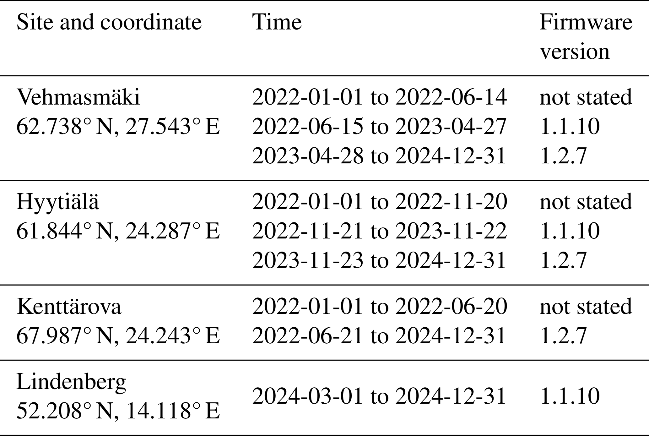
Data collected up to December 2024 from four CL61 deployed at four different ACTRIS Cloudnet sites were analyzed. Three of these instruments are situated in Finland: Hyytiälä, Vehmasmäki, and Kenttärova, while the fourth is located in Lindenberg, Germany. The firmware versions of the instruments (i.e., 1.1.10 and 1.2.7), along with their respective periods of validity, are presented in Table 2. The data from this study were obtained from the ACTRIS Cloudnet data portal (Görsdorf et al., 2025).

Table 2 Firmware version of the CL61 across all the site locations.

The CL61 is equipped with an internal heater to stabilize the temperatures of the laser and optical components. It includes a window heater and blower to maintain stable window conditions, as the window's transmission efficiency significantly affects the backscattered signal (see Sect. 4.3). The instrument's firmware continuously monitors and reports various housekeeping variables, such as internal temperature, laser temperature, window condition (calculated internally on a scale from 0 % for a fully obstructed window to 100 % for a clean window), and the status of the window blower heater. The quantity and type of variables reported may differ based on the firmware version.

3 Methods

The CL61 operates by emitting pulses of linear polarized laser light into the atmosphere and recording the backscattered signal. The received power per laser pulse is described by the lidar equation (Wandinger, 2005):

$$\begin{array}{}\text{(1)}& P\left(r\right)={\displaystyle \frac{\mathrm{1}}{r^{\mathrm{2}}}}{C}_{\mathrm{L}}O\left(r\right)\mathit{\beta }\left(r\right)e^{-\mathrm{2}{\int }_{\mathrm{0}}^r\mathit{\alpha }\left(r^{\prime }\right)\mathrm{d}{r}^{\prime }}+B.\end{array}$$

Here, O(r) is the overlap function that is unique to each instrument and is provided by the manufacturer. The coefficients α and β represent atmospheric extinction and backscatter, respectively, B is the background signal, and C_L represents the lidar constant. This constant encapsulates the system-specific characteristics of the lidar, such as its receiver optics and laser properties. It is initially determined and provided by the manufacturer, but it may drift over time as the instrument ages and its performance changes. Although the internal firmware attempts to monitor and compensate for these changes, additional calibration, such as absolute calibration using stratocumulus clouds (O'Connor et al., 2004; Hopkin et al., 2019), is still necessary.

The instrument provides two main output signals, ppol and xpol, in arbitrary units [a.u.], as they are reported prior to absolute calibration. These paremters represent the estimated normalized and background-, range- and overlap-corrected parallel- and cross-polarized components of the attenuated backscattered signal (${}^{\parallel }{\mathit{\beta }}^{\prime }$ and ${}^{⟂}{\mathit{\beta }}^{\prime }$ respectively). They can be defined as:

$$\begin{array}{}\text{(2)}& {\displaystyle }\text{ppol}{=}^{\parallel }{\displaystyle \frac{\left(P\right(r)-B_{\mathrm{estimated}})r^{\mathrm{2}}}{C_{\mathrm{L}}O\left(r\right)}}{=}^{\parallel }{\mathit{\beta }}^{\prime },\text{(3)}& {\displaystyle }\text{xpol}{=}^{⟂}{\displaystyle \frac{\left(P\left(r\right)-B_{\mathrm{estimated}}\right)r^{\mathrm{2}}}{C_{\mathrm{L}}O\left(r\right)}}{=}^{⟂}{\mathit{\beta }}^{\prime },\end{array}$$

where B_estimated is the internally estimated background signal by the instrument. The instrument also provides the total attenuated backscatter signal, which is the sum of the attenuated backscatter from all polarizations:

$$\begin{array}{}\text{(4)}& {\mathit{\beta }}^{\prime }{=}^{\parallel }{\mathit{\beta }}^{\prime }{+}^{⟂}{\mathit{\beta }}^{\prime },\end{array}$$

and the volume linear depolarization ratio being:

$$\begin{array}{}\text{(5)}& {\mathit{\delta }}_{\mathrm{v}}={\displaystyle \frac{{}^{⟂}{\mathit{\beta }}^{\prime }}{{}^{\parallel }{\mathit{\beta }}^{\prime }}}.\end{array}$$

3.1 Residual background signal

The observed backscattered signal detected by a lidar consists of the true atmospheric signal and the background signal (Cao et al., 2013). The true atmospheric signal consists of backscattered contributions from particles (β_p) and molecular scattering (β_mol), whilst the background signal includes contributions from both atmospheric background signal P_atmosphere (such as solar radiation, moonlight, or artificial light) and instrumental background P_instrument signal (dark signal). Although the instrument already determines and performs the background correction internally, residual background components may still remain in the measured signal, such as the dark signal observed during termination hood measurements (see Sect. 3.1.1). Therefore, we extend Eqs. (2) and (3) to account for the residual background signal (hereafter referred to as the background signal), B_res, that is not removed by the internal correction:

$$\begin{array}{}\text{(6)}& {\displaystyle }\begin{array}{rl}{}^{\parallel }{\mathit{\beta }}^{\prime }& {=}^{\parallel }{\displaystyle \frac{\left(P\right(r)-B_{\mathrm{estimated}})r^{\mathrm{2}}}{C_{\mathrm{L}}O\left(r\right)}}{+}^{\parallel }{\displaystyle \frac{B_{\mathrm{res}}\left(r\right)r^{\mathrm{2}}}{C_{\mathrm{L}}O\left(r\right)}}\\ & {=}^{\parallel }{\mathit{\beta }}_{\mathrm{corrected}}^{\prime }{+}^{\parallel }{\displaystyle \frac{B_{\mathrm{res}}\left(r\right)r^{\mathrm{2}}}{C_{\mathrm{L}}O\left(r\right)}},\end{array}\text{(7)}& {\displaystyle }\begin{array}{rl}{}^{⟂}{\mathit{\beta }}^{\prime }& {=}^{⟂}{\displaystyle \frac{\left(P\right(r)-B_{\mathrm{estimated}})r^{\mathrm{2}}}{C_{\mathrm{L}}O\left(r\right)}}{+}^{⟂}{\displaystyle \frac{B_{\mathrm{res}}\left(r\right)r^{\mathrm{2}}}{C_{\mathrm{L}}O\left(r\right)}}\\ & {=}^{⟂}{\mathit{\beta }}_{\mathrm{corrected}}^{\prime }{+}^{⟂}{\displaystyle \frac{B_{\mathrm{res}}\left(r\right)r^{\mathrm{2}}}{C_{\mathrm{L}}O\left(r\right)}}.\end{array}\end{array}$$

To eliminate the range dependence from the background terms, we divide each expression by r², yielding:

$$\begin{array}{}\text{(8)}& {\displaystyle \frac{{}^{\parallel }{\mathit{\beta }}^{\prime }}{r^{\mathrm{2}}}}={\displaystyle \frac{{}^{\parallel }{\mathit{\beta }}_{\mathrm{corrected}}^{\prime }}{r^{\mathrm{2}}}}{+}^{\parallel }{\displaystyle \frac{B_{\mathrm{res}}\left(r\right)}{C_{\mathrm{L}}O\left(r\right)}},\text{(9)}& {\displaystyle \frac{{}^{⟂}{\mathit{\beta }}^{\prime }}{r^{\mathrm{2}}}}={\displaystyle \frac{{}^{⟂}{\mathit{\beta }}_{\mathrm{corrected}}^{\prime }}{r^{\mathrm{2}}}}{+}^{⟂}{\displaystyle \frac{B_{\mathrm{res}}\left(r\right)}{C_{\mathrm{L}}O\left(r\right)}}.\end{array}$$

For simplicity, we define the background terms as:

$$\begin{array}{}\text{(10)}& P_{\mathrm{res}}\left(r\right)\equiv {\displaystyle \frac{B_{\mathrm{res}}\left(r\right)}{C_{\mathrm{L}}O\left(r\right)}},\end{array}$$

where P_res(r) = P_atmosphere(r)+P_instrument(r).

To derive the ${\mathit{\beta }}_{\mathrm{corrected}}^{\prime }$, the background signals need to be quantified. Since the measured ${}^{\parallel }{\mathit{\beta }}^{\prime }$ and ${}^{⟂}{\mathit{\beta }}^{\prime }$ signals include contributions from background signal in their respective polarization channels, it is necessary to estimate the background signal separately for each polarization (^∥P_res and ^⟂P_res). To achieve this, a background identification methodology has been developed. It identifies regions within the dataset that are free of aerosols and hydrometeors, where the $\frac{{}^{\parallel }{\mathit{\beta }}^{\prime }}{r^{\mathrm{2}}}$ and $\frac{{}^{⟂}{\mathit{\beta }}^{\prime }}{r^{\mathrm{2}}}$ values are assumed to predominantly represent background signal.

The methodology proceeds as follows. First, the data is averaged over 5 min intervals. The $\frac{{}^{\parallel }{\mathit{\beta }}^{\prime }}{r^{\mathrm{2}}}$ and $\frac{{}^{⟂}{\mathit{\beta }}^{\prime }}{r^{\mathrm{2}}}$ profiles are then decomposed using the stationary wavelet transform (SWT) with the bior.1 wavelet, implemented via PyWavelets (Nason and Silverman, 1995; Lee et al., 2019). Subsequently, the background signal variance is reduced by applying a hard-threshold shrinkage function to the approximation and detail coefficients from levels 1 through 7, using minimax thresholding (Nason and Silverman, 1995). The profile is reconstructed via the inverse stationary wavelet transform. Finally, the background range gates are identified as regions with values below half of the previously computed minimax threshold. The mean and variance of the background are computed from the original, non-averaged data with the identified background range gates using 5 min time intervals and 2 km range-bin intervals.

An example of this methodology applied to data in Kenttärova on 28 March 2024 is illustrated in Fig. 1. During daylight hours, solar radiation significantly increases the variance (${\mathit{\sigma }}_{{}^{\parallel }{P}_{\mathrm{res}}}^{\mathrm{2}}$ and ${\mathit{\sigma }}_{{}^{⟂}{P}_{\mathrm{res}}}^{\mathrm{2}}$) of the background signal, resulting in a daytime variance much higher than that observed at night, as shown in panels (g) and (h). Above the aerosol and cloud layers, both the mean (${\mathit{\mu }}_{{}^{\parallel }{P}_{\mathrm{res}}}$ and ${\mathit{\mu }}_{{}^{⟂}{P}_{\mathrm{res}}}$) and variance of the background signals in both polarizations remain relatively stable with range, or at least exhibit considerably smaller variations compared to the diurnal fluctuations.

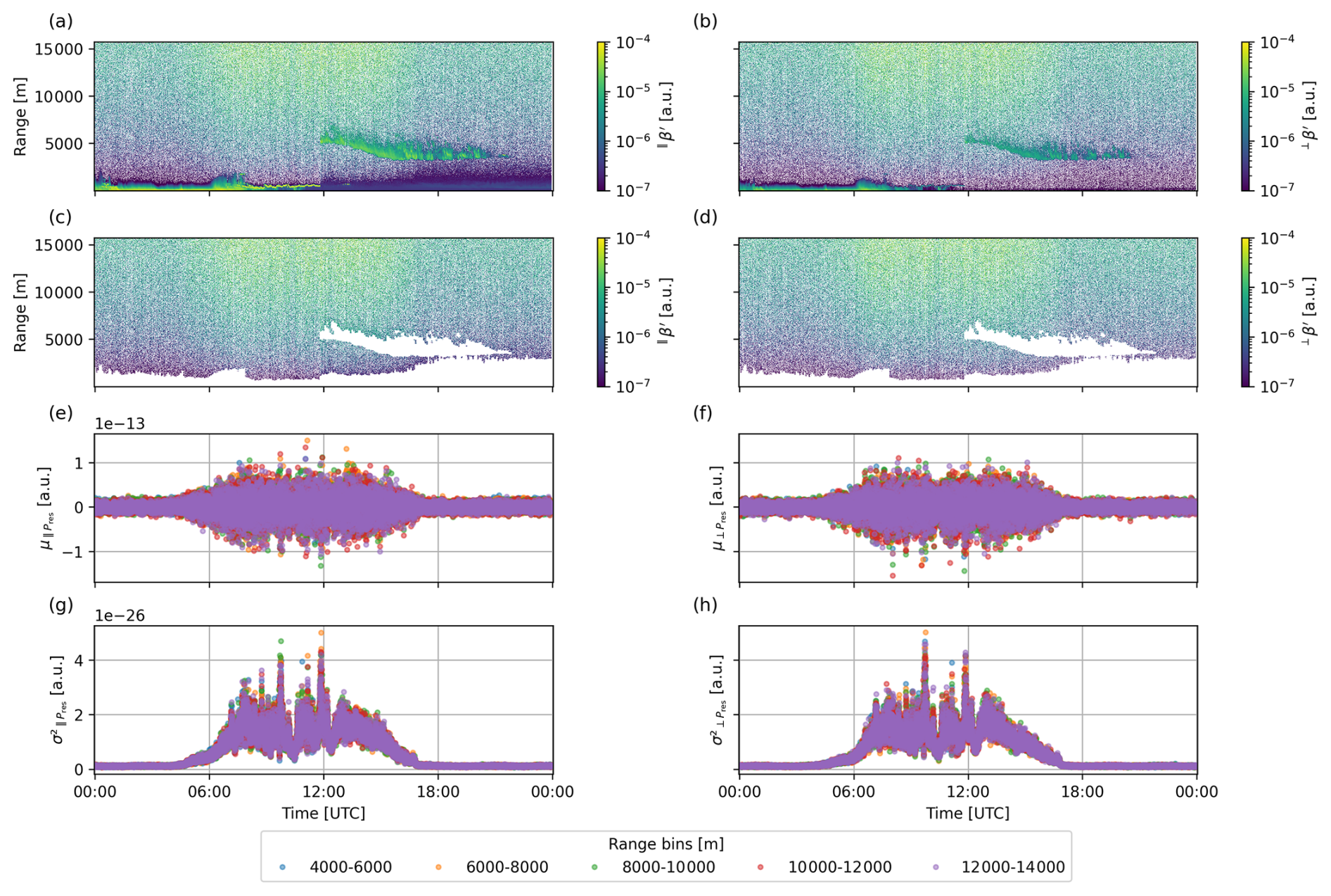
Figure 1 Time series from Kenttärova on 28 March 2024 showing: (a) ${}^{\parallel }{\mathit{\beta }}^{\prime }$, (b) ${}^{⟂}{\mathit{\beta }}^{\prime }$, (c) background ${}^{\parallel }{\mathit{\beta }}^{\prime }$, and (d) background ${}^{⟂}{\mathit{\beta }}^{\prime }$. Panels (e) to (h) display the background at different range bins from 4000 to 6000, 6000 to 8000, 8000 to 10 000, 10 000 to 12 000, and 12 000 to 14 000 m, with color indicating the range bin: (e) ${\mathit{\mu }}_{{}^{\parallel }{P}_{\mathrm{res}}}$, (f) ${\mathit{\mu }}_{{}^{⟂}{P}_{\mathrm{res}}}$, (g) ${\mathit{\sigma }}_{{}^{\parallel }{P}_{\mathrm{res}}}^{\mathrm{2}}$, and (h) ${\mathit{\sigma }}_{{}^{⟂}{P}_{\mathrm{res}}}^{\mathrm{2}}$. These parameters are computed at a 10 s temporal resolution using all data within each range bin.

By applying this methodology to the full dataset, we obtained the time series of P_res for all instruments in both polarizations. Comparing these background signals with other housekeeping parameters, such as laser power, enables us to evaluate the operational performance of each instrument. Moreover, since each background component is quantified independently, we can correct the signal and estimate its uncertainty in both polarizations ${}^{\parallel }{\mathit{\beta }}^{\prime }$ and ${}^{⟂}{\mathit{\beta }}^{\prime }$ and, consequently, in the derived linear depolarization ratio.

3.1.1 Instrumental background signal

To obtain the instrumental background signal, a termination hood (Vaisala CL61TERMHOOD) was placed over the window of each ceilometer located in Finland (Fig. 2). The hood was applied without modifying the instrument's internal operating parameters, ensuring that all measurements reflected normal operational conditions. The hood's material and design totally attenuate the outgoing laser beam, preventing any backscatter signal from reaching the detector. As a result, the measured signal can be attributed entirely to the instrumental background signal adjusted by the overlap correction. Although the overlap correction remains constant for each instrument, it was reverted to accurately interpret the instrumental background signal in the near range P_instrumentO(r).

Figure 2 A termination hood (Vaisala CL61TERMHOOD) place on top of the CL61 in Hyytiälä.

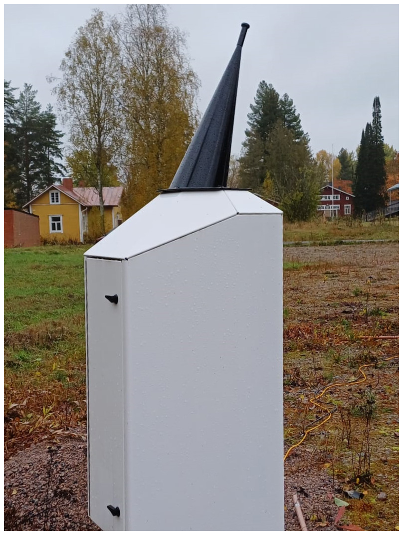
Figure 3 presents example profiles of ${}^{\parallel }{\mathit{\beta }}^{\prime }$ and ${}^{⟂}{\mathit{\beta }}^{\prime }$ both before and during the termination hood measurements. Before the termination hood was applied, the ${\mathit{\mu }}_{{}^{\parallel }{\mathit{\beta }}^{\prime }}$ and ${\mathit{\mu }}_{{}^{⟂}{\mathit{\beta }}^{\prime }}$ profiles in the aerosol and hydrometeor-free region above 5 km closely follow the theoretical molecular attenuated backscatter coefficient ${\mathit{\beta }}_{\mathrm{mol}}^{\prime }$ (Fig. 3b and c), indicating that the CL61 is sensitive to molecular scattering. The ${\mathit{\beta }}_{\mathrm{mol}}^{\prime }$ profile was calculated following the method described by Bucholtz (1995) using meteorological input data from a numerical weather prediction model available from the ACTRIS Cloudnet data portal (O'Connor, 2025). At ranges above 10 km, however, the molecular signal becomes indistinguishable from noise. The variance profiles, ${\mathit{\sigma }}_{{}^{\parallel }{\mathit{\beta }}^{\prime }/r^{\mathrm{2}}}^{\mathrm{2}}$ and ${\mathit{\sigma }}_{{}^{⟂}{\mathit{\beta }}^{\prime }/r^{\mathrm{2}}}^{\mathrm{2}}$, also remain relatively constant in this region (Fig. 3f and g).

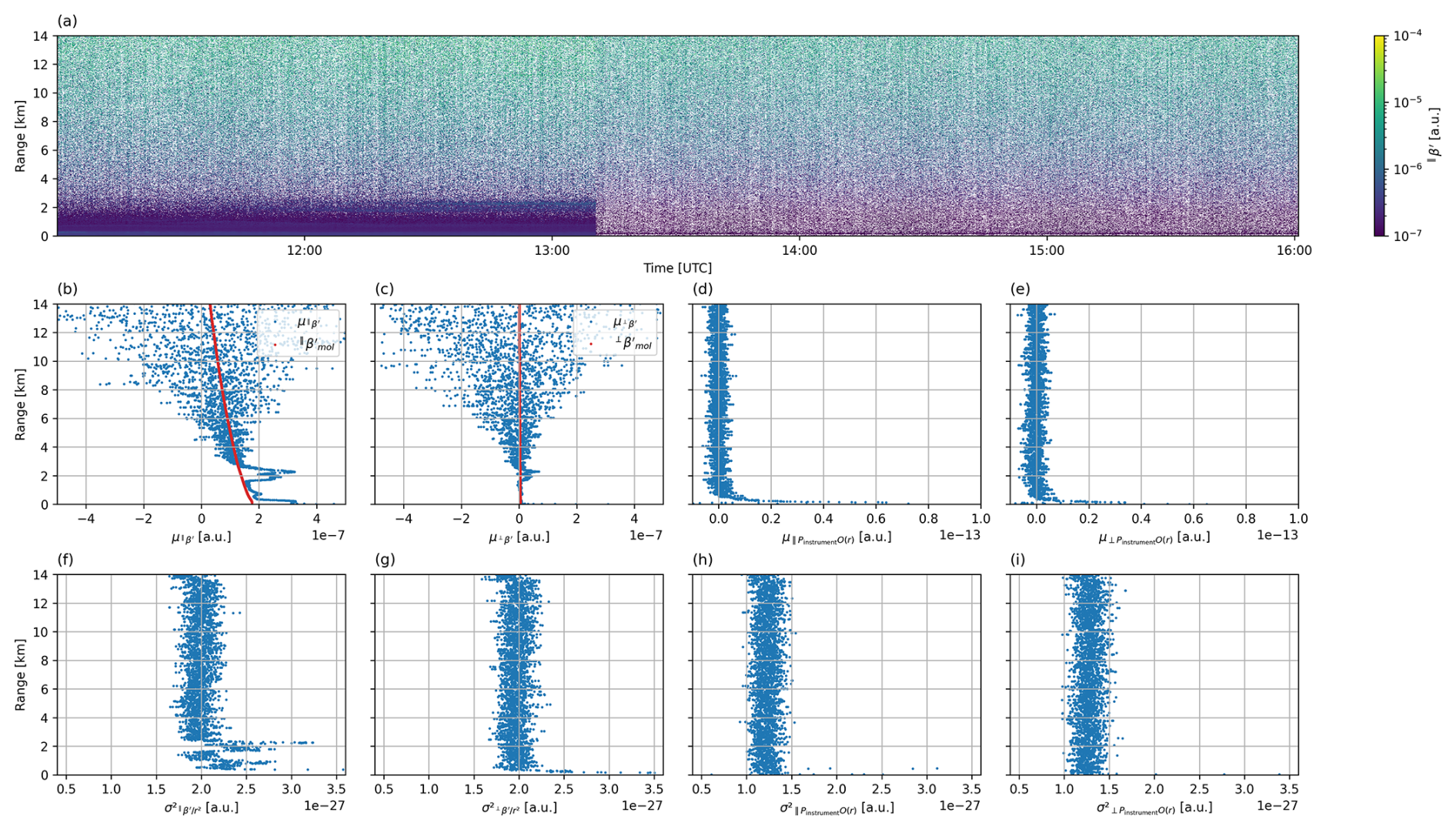
Figure 3 Measurements at Kenttärova on 5 March 2024. (a) The time series of ${}^{\parallel }{\mathit{\beta }}^{\prime }$. Panels (b), (c), (f), and (g) display the averaged profiles in time at each range gate before the termination hood measurement (from 11:00 to 13:00 UTC): (b) ${\mathit{\mu }}_{{}^{\parallel }{\mathit{\beta }}^{\prime }}$ and $\parallel {\mathit{\beta }}_{\mathrm{mol}}^{\prime }$, (c) ${\mathit{\mu }}_{{}^{⟂}{\mathit{\beta }}^{\prime }}$ and $⟂{\mathit{\beta }}_{\mathrm{mol}}^{\prime }$, (f) ${\mathit{\sigma }}_{{}^{\parallel }{\mathit{\beta }}^{\prime }/r^{\mathrm{2}}}^{\mathrm{2}}$, (g) ${\mathit{\sigma }}_{{}^{⟂}{\mathit{\beta }}^{\prime }/r^{\mathrm{2}}}^{\mathrm{2}}$. Panels (d), (e), (h) and (i) display the averaged profiles in time at each range gate during the termination hood measurement at 19 °C (from 14:00 to 15:00 UTC): (d) ${\mathit{\mu }}_{{}^{\parallel }{P}_{\mathrm{instrument}}O\left(r\right)}$, (e) ${\mathit{\mu }}_{{}^{⟂}{P}_{\mathrm{instrument}}O\left(r\right)}$, (h) ${\mathit{\sigma }}_{{}^{\parallel }{P}_{\mathrm{instrument}}O\left(r\right)}^{\mathrm{2}}$, (i) ${\mathit{\sigma }}_{{}^{⟂}{P}_{\mathrm{instrument}}O\left(r\right)}^{\mathrm{2}}$.

During the termination hood measurement, ${\mathit{\mu }}_{P_{\mathrm{instrument}}O\left(r\right)}$ from both polarizations remains relatively stable above 1.2 km, but increases significantly below this range (Fig. 3d, e). This increase suggests the presence of a signal bias at lower ranges that has not been corrected by the firmware and will be investigated in this study. Additionally, a reduction in the signal variance of both polarization channels is observed during the termination hood measurement (Fig. 3h, i) compared to the previous period above the complete overlap range. This reduction is attributed to the absence of solar influence during the termination hood measurement.

In principle, the nighttime measurements could be used to estimate P_instrument. However, only the portion of the P_instrument profile at higher ranges, where clouds and aerosols are absent, can be reliably estimated. An example is shown in Fig. S2, where ${\mathit{\sigma }}_{{}^{\parallel }{\mathit{\beta }}^{\prime }/r^{\mathrm{2}}}^{\mathrm{2}}$ agrees well between the hood termination and nighttime measurements only at ranges above approximately 2 km. This agreement is observed only under clear-sky conditions, as cloud layers at lower ranges can increase the measured background values.

Since the CL61 is a coaxial lidar, it is prone to the afterpulsing effect, such as those caused by internal reflections of the outgoing laser beam that reach the detector (Campbell et al., 2002; Welton and Campbell, 2002). Hervo et al. (2016) demonstrated that the overlap function for a ceilometer made by another manufacturer (Lufft CHM15k) was sensitive to the instrument internal temperature, T, mainly due to temperature-induced changes in its optical components. It is likely that the observed bias is temperature-dependent and is caused by variations in instrumental background associated with afterpulsing, dark signal, and optical components under different temperature conditions. To quantify the effect of temperature, the termination hood measurement was repeated over a range of internal temperatures T, reported as internal_temperature in the instrument housekeeping data, across a two-year period. Hence, the instrumental background signal mean (bias) and its variance (noise) from both polarizations with respect to internal temperature can be determined.

3.1.2 Atmospheric background signal

For an accurate estimation of the background signal, the contribution from the atmospheric background signal, P_atmosphere, must be taken into account. As noted by Kotthaus et al. (2016), earlier instruments such as the CL31 incorporate a zero-bias level that compensates for temporal fluctuations in solar radiation. This is also evident in CL61 as shown in Fig. 3b and c, where the ${\mathit{\mu }}_{{}^{\parallel }{\mathit{\beta }}^{\prime }}$ and ${\mathit{\mu }}_{{}^{⟂}{\mathit{\beta }}^{\prime }}$ values above 5 km closely follow β_mol, confirming the zero-mean solar radiation noise. Therefore, the firmware must have corrected the atmospheric background signal to a zero mean, leaving only its variance (noise) contributing to the background signal, which will be addressed in this study.

The solar noise variance can be seen from the diurnal pattern in Fig. 1g and h; and the difference between the σ² profiles before (Fig. 3f and g) and during (Fig. 3h and i) the termination hood measurement. Since this difference remains approximately constant at all ranges above the aerosol layer near the ground, we assume that the atmospheric background variance from both polarizations, ${\mathit{\sigma }}_{P_{\mathrm{atmosphere}}}^{\mathrm{2}}$, is also uniform down to the near range. Then, ${\mathit{\sigma }}_{P_{\mathrm{atmosphere}}}^{\mathrm{2}}$ is calculated by computing the difference between the variance of the background signal ${\mathit{\sigma }}_{P_{\mathrm{res}}}^{\mathrm{2}}$ (obtained between 10 and 12 km using the background identification methodology) and the variance of the instrumental background signal ${\mathit{\sigma }}_{P_{\mathrm{instrument}}}^{\mathrm{2}}$ (obtained at the same range and temperature from the termination hood measurement):

$$\begin{array}{}\text{(11)}& {\mathit{\sigma }}_{P_{\mathrm{atmosphere}}}^{\mathrm{2}}={\mathit{\sigma }}_{P_{\mathrm{res}}(r=\mathrm{10}-\mathrm{12}\mathrm{km})}^{\mathrm{2}}-{\mathit{\sigma }}_{P_{\mathrm{instrument}}(r=\mathrm{10}-\mathrm{12}\mathrm{km},T)}^{\mathrm{2}}.\end{array}$$

Here, ${\mathit{\sigma }}_{P_{\mathrm{atmosphere}}}^{\mathrm{2}}$ is independent of the range and is obtained separately for each polarization in each individual profile.

3.1.3 Correction for systematic bias

After measuring P_instrument(r,T) across a range of T during the termination hood measurements, the results are stored as a lookup table containing P_instrument(r,T) profiles at each T. The attenuated backscatter coefficient for each polarization can be corrected by applying the P_instrument(r,T) value corresponding to the instrument's current internal temperature as follows:

$$\begin{array}{}\text{(12)}& {}^{\parallel }{\mathit{\beta }}_{\mathrm{corrected}}^{\prime }{=}^{\parallel }{\mathit{\beta }}^{\prime }-{\mathit{\mu }}_{{}^{\parallel }{P}_{\mathrm{instrument}}(r,T)}{r}^{\mathrm{2}},\text{(13)}& {}^{⟂}{\mathit{\beta }}_{\mathrm{corrected}}^{\prime }{=}^{⟂}{\mathit{\beta }}^{\prime }-{\mathit{\mu }}_{{}^{⟂}{P}_{\mathrm{instrument}}(r,T)}{r}^{\mathrm{2}},\end{array}$$

and their corresponding uncertainties are given by:

$$\begin{array}{}\text{(14)}& {\displaystyle }{\mathit{\sigma }}_{{}^{\parallel }{\mathit{\beta }}_{\mathrm{corrected}}^{\prime }}^{\mathrm{2}}=\left({\mathit{\sigma }}_{{}^{\parallel }{P}_{\mathrm{atmosphere}}}^{\mathrm{2}}+{\mathit{\sigma }}_{{}^{\parallel }{P}_{\mathrm{instrument}}(r,T)}^{\mathrm{2}}\right)r^{\mathrm{2}},\text{(15)}& {\displaystyle }{\mathit{\sigma }}_{{}^{⟂}{\mathit{\beta }}_{\mathrm{corrected}}^{\prime }}^{\mathrm{2}}=({\mathit{\sigma }}_{{}^{⟂}{P}_{\mathrm{atmosphere}}}^{\mathrm{2}}+{\mathit{\sigma }}_{{}^{⟂}{P}_{\mathrm{instrument}}(r,T)}^{\mathrm{2}})r^{\mathrm{2}}.\end{array}$$

The bias-corrected attenuated backscatter coefficient and volume linear depolarization ratio are then calculated as:

$$\begin{array}{}\text{(16)}& {\displaystyle }{\mathit{\beta }}_{\mathrm{corrected}}^{\prime }{=}^{\parallel }{\mathit{\beta }}_{\mathrm{corrected}}^{\prime }{+}^{⟂}{\mathit{\beta }}_{\mathrm{corrected}}^{\prime },\text{(17)}& {\displaystyle }{\mathit{\delta }}_{\mathrm{corrected}}={\displaystyle \frac{{}^{⟂}{\mathit{\beta }}_{\mathrm{corrected}}^{\prime }}{{}^{\parallel }{\mathit{\beta }}_{\mathrm{corrected}}^{\prime }}},\end{array}$$

and their associated uncertainty, given by

$$\begin{array}{}\text{(18)}& {\displaystyle }{\mathit{\sigma }}_{{\mathit{\beta }}_{\mathrm{corrected}}^{\prime }}^{\mathrm{2}}={\mathit{\sigma }}_{{}^{\parallel }{\mathit{\beta }}_{\mathrm{corrected}}^{\prime }}^{\mathrm{2}}+{\mathit{\sigma }}_{{}^{⟂}{\mathit{\beta }}_{\mathrm{corrected}}^{\prime }}^{\mathrm{2}},\text{(19)}& {\displaystyle }{\mathit{\sigma }}_{{\mathit{\delta }}_{\mathrm{corrected}}}^{\mathrm{2}}={\mathit{\delta }}^{\mathrm{2}}\left({\displaystyle \frac{{\mathit{\sigma }}_{{}^{⟂}{\mathit{\beta }}_{\mathrm{corrected}}^{\prime }}^{\mathrm{2}}}{{}^{⟂}{\mathit{\beta }}_{\mathrm{corrected}}^{\prime \mathrm{2}}}}+{\displaystyle \frac{{\mathit{\sigma }}_{{}^{\parallel }{\mathit{\beta }}_{\mathrm{corrected}}^{\prime }}^{\mathrm{2}}}{{}^{\parallel }{\mathit{\beta }}_{\mathrm{corrected}}^{\prime \mathrm{2}}}}\right).\end{array}$$

3.2 Calibration

To ensure the CL61 produces a consistent and accurate backscatter signal, the ceilometer signal must be manually calibrated in addition to its internal calibration. This involves calibrating the backscatter signal from the CL61 using a reference target with known backscatter characteristics. Two commonly used calibration methods for deriving C_L are based on different types of reference targets: atmospheric molecules (Rayleigh calibration) and liquid clouds (liquid cloud calibration).

The Rayleigh calibration (Fernald et al., 1972; Klett, 1985; Binietoglou et al., 2011; Wiegner and Geiß, 2012; Baars et al., 2016), often referred to as the backward inversion approach, is the standard method to derive the particle backscatter coefficient (β_p) for most research aerosol lidars due to their sensitivity to molecular signal (Wiegner et al., 2014). As illustrated in Fig. 3b, the attenuated backscatter coefficient profile from CL61 closely follows the attenuated molecular backscatter coefficient above the aerosol layer at 4 km. This indicates a significant contribution of molecular scattering to the total CL61 signal, especially in aerosol- and hydrometeor-free regions. Therefore, the Rayleigh calibration can be applied to the CL61, provided a sufficiently long averaging time (more than 2 h) is used.

The Rayleigh calibration method requires an assumed lidar ratio for aerosol particles (S_p). At sites equipped with a sun photometer, S_p can be constrained (Wiegner and Geiß, 2012); otherwise, a value of 50 sr was used. The first 50 m range has been discarded due to unreliable data (see Sect. 4.5), and it has been demonstrated that the resulting loss in optical depth for ignoring near range gates is negligible (Wiegner and Geiß, 2012). After the β_p profile is derived, the lidar constant C_L can be determined from the lidar equation (Wiegner and Geiß, 2012).

The liquid cloud calibration (O'Connor et al., 2004; Hopkin et al., 2019) relies on the fact that the lidar ratio for liquid water clouds at the ceilometer wavelength is known. This method involves calculating the integrated attenuated backscatter coefficient for fully attenuated liquid water clouds, including the contribution from multiple scattering. The theoretical contribution from multiple scattering is computed for droplet diameters ranging from 8 to 20 µm, taking into account the CL61 beam divergence and receiver field of view. The integrated backscatter coefficient is then scaled to fit within the expected theoretical values. This scaling factor is the calibration factor C, which is the reciprocal of the lidar constant C_L. The primary advantage of this approach over Rayleigh calibration is the substantially higher signal-to-noise ratio of the backscatter from water clouds compared to the molecular backscatter. As a result, it eliminates the need for long nighttime averaging periods required to obtain a reliable molecular signal.

A methodology was developed to identify suitable liquid cloud profiles. First, a representative liquid cloud profile containing a single liquid cloud layer and exhibiting complete signal attenuation approximately 200 m above the cloud base was selected as the reference profile. Each β^′ profile in the dataset was then cross-correlated with this reference to quantify their similarity. For each time step, the height corresponding to the maximum cross-correlation value was identified as the most similar location and treated as a pseudo in-cloud height. Next, the ratio of total in-cloud β^′, calculated over a 150 m layer centered at the pseudo in-cloud height, to the integrated β^′ of the entire profile was computed. A profile was classified as containing a liquid cloud if this ratio exceeded 90 %, ensuring that the integrated β^′ was not significantly influenced by strong aerosol loading or precipitation. Additionally, the cross-correlation value at the identified height was required to exceed 5 × 10⁻⁷. This threshold was selected to ensure that at least 1000 valid data points were available for each month.

To ensure robust data fitting, the cloud calibration is performed monthly using all suitable liquid cloud observations detected from the methodology. To validate the cloud calibration results, Rayleigh calibration was also computed occasionally when possible. Data from a co-located sun photometer was used to constrain the lidar ratio for Rayleigh calibration. If no sun photometer data is available, a lidar ratio of 50 sr is used.

The calibrated volume attenuated backscatter coefficient and its uncertainty can then be determined as follows, assuming the cloud calibration factor has an uncertainty of approximately 10 % (Hopkin et al., 2019):

$$\begin{array}{}\text{(20)}& {\displaystyle }{\mathit{\beta }}_{\mathrm{v}}^{\prime }={\mathit{\beta }}_{\mathrm{corrected}}^{\prime }\cdot C,\text{(21)}& {\displaystyle }{\mathit{\sigma }}_{{\mathit{\beta }}_{\mathrm{v}}^{\prime }}^{\mathrm{2}}=\left({\mathit{\sigma }}_{{\mathit{\beta }}_{\mathrm{corrected}}^{\prime }}^{\mathrm{2}}+\mathrm{0.01}\cdot {\mathit{\beta }}_{\mathrm{corrected}}^{\prime \mathrm{2}}\right)\cdot C^{\mathrm{2}}.\end{array}$$

For those instruments where termination hood measurements are not available:

$$\begin{array}{}\text{(22)}& {\displaystyle }{\mathit{\beta }}_{\mathrm{v}}^{\prime }={\mathit{\beta }}^{\prime }\cdot C,\text{(23)}& {\displaystyle }\begin{array}{rl}{\mathit{\sigma }}_{{\mathit{\beta }}_{\mathrm{v}}^{\prime }}^{\mathrm{2}}& =\left({\mathit{\sigma }}_{P_{\mathrm{atmosphere}}}^{\mathrm{2}}+\mathrm{0.01}\cdot {\mathit{\beta }}^{\prime \mathrm{2}}\right)\cdot C^{\mathrm{2}}\\ & =\left({\mathit{\sigma }}_{{}^{\parallel }{P}_{\mathrm{atmosphere}}}^{\mathrm{2}}+{\mathit{\sigma }}_{{}^{⟂}{P}_{\mathrm{atmosphere}}}^{\mathrm{2}}+\mathrm{0.01}\cdot {\mathit{\beta }}^{\prime \mathrm{2}}\right)\cdot C^{\mathrm{2}}.\end{array}\end{array}$$

The calibration is assumed to affect both polarization channels equally. Hence, δ_corrected remains unchanged.

3.3 Aerosol particle inversion

The particle backscatter coefficient profile (β_p) is retrieved using the forward Klett solution (Klett, 1985) after applying the previously derived cloud calibration factor and assuming that the instrument does not undergo significant degradation within a one-month period. Similar to the previous section, the first 50 m range has been discarded. The cloud calibration factor is estimated to have an uncertainty of approximately 10 % (Hopkin et al., 2019). The forward inversion does not require extensive temporal averaging. When available, sun photometer observations are used to constrain the lidar ratio S_p; otherwise, a constant value of 50 sr is applied to all aerosol layers in the retrieval.

Let ${\mathit{\beta }}_{\mathrm{p}}=f({\mathit{\beta }}_{\mathrm{v}}^{\prime },C,S_{\mathrm{p}})$ represent the inversion function; then the uncertainty of β_p is calculated as

$$\begin{array}{}\text{(24)}& {\mathit{\sigma }}_{{\mathit{\beta }}_{\mathrm{p}}}^{\mathrm{2}}={\left({\displaystyle \frac{\partial f}{\partial {\mathit{\beta }}_{\mathrm{v}}^{\prime }}}{\mathit{\sigma }}_{{\mathit{\beta }}_{\mathrm{v}}^{\prime }}\right)}^{\mathrm{2}}+{\left({\displaystyle \frac{\partial f}{\partial C}}{\mathit{\sigma }}_C\right)}^{\mathrm{2}}+{\left({\displaystyle \frac{\partial f}{\partial S}}{\mathit{\sigma }}_{S_{\mathrm{p}}}\right)}^{\mathrm{2}}.\end{array}$$

The partial derivatives can be approximated using central differences:

$$\begin{array}{}\text{(25)}& {\displaystyle \frac{\partial f}{\partial {\mathit{\beta }}_{\mathrm{v}}^{\prime }}}{\mathit{\sigma }}_{{\mathit{\beta }}_{\mathrm{v}}^{\prime }}\approx {\displaystyle \frac{f\left({\mathit{\beta }}_{\mathrm{v}}^{\prime }+{\mathit{\sigma }}_{{\mathit{\beta }}_{\mathrm{v}}^{\prime }},C,S_{\mathrm{p}}\right)-f\left({\mathit{\beta }}_{\mathrm{v}}^{\prime }-{\mathit{\sigma }}_{{\mathit{\beta }}_{\mathrm{v}}^{\prime }},C,S_{\mathrm{p}}\right)}{\mathrm{2}}},\text{(26)}& {\displaystyle \frac{\partial f}{\partial C}}{\mathit{\sigma }}_C\approx {\displaystyle \frac{f\left({\mathit{\beta }}_{\mathrm{v}}^{\prime },C_{max},S_{\mathrm{p}}\right)-f\left({\mathit{\beta }}_{\mathrm{v}}^{\prime },C_{min},S_{\mathrm{p}}\right)}{\mathrm{2}}},\text{(27)}& {\displaystyle \frac{\partial f}{\partial S}}{\mathit{\sigma }}_{S_{\mathrm{p}}}\approx {\displaystyle \frac{f\left({\mathit{\beta }}_{\mathrm{v}}^{\prime },C,S_{\mathrm{p},max}\right)-f\left({\mathit{\beta }}_{\mathrm{v}}^{\prime },C,S_{\mathrm{p},min}\right)}{\mathrm{2}}}\end{array}$$

with $C_{min}=\mathrm{0.9}\cdot C$, $C_{max}=\mathrm{1.1}\cdot C$, $S_{\mathrm{p},min}=S_{\mathrm{p}}-\mathrm{10}$, and $S_{\mathrm{p},min}=S_{\mathrm{p}}+\mathrm{10}$

Following (Biele et al., 2000; Freudenthaler et al., 2009), the particle linear depolarization ratio (δ_p) is then obtained as

$$\begin{array}{}\text{(28)}& {\mathit{\delta }}_{\mathrm{p}}={\displaystyle \frac{\left(\mathrm{1}+{\mathit{\delta }}_{\mathrm{m}}\right){\mathit{\delta }}_{\mathrm{v}}R-\left(\mathrm{1}+{\mathit{\delta }}_{\mathrm{v}}\right){\mathit{\delta }}_{\mathrm{m}}}{\left(\mathrm{1}+{\mathit{\delta }}_{\mathrm{m}}\right)R-\left(\mathrm{1}+{\mathit{\delta }}_{\mathrm{v}}\right)}},\end{array}$$

where the backscatter ratio R is defined as

$$\begin{array}{}\text{(29)}& R={\displaystyle \frac{{\mathit{\beta }}_{\mathrm{p}}+{\mathit{\beta }}_{\mathrm{m}}}{{\mathit{\beta }}_{\mathrm{m}}}},\end{array}$$

and δ_v is the volume linear depolarization ratio, which is δ_corrected in Eq. (17), or $\frac{{}^{⟂}{\mathit{\beta }}^{\prime }}{{}^{\parallel }{\mathit{\beta }}^{\prime }}$ for instruments lacking termination hood measurements.

The molecular depolarization ratio (δ_m) is estimated following Tomasi et al. (2005), accounting for major atmospheric gases and the influence of water vapor. The input data for these calculations are taken from a numerical weather prediction model (ECMWF IFS forecast) provided via the ACTRIS Cloudnet data portal (O'Connor, 2025).

The uncertainty of δ_p can be determined using partial derivatives

$$\begin{array}{}\text{(30)}& {\mathit{\sigma }}_{{\mathit{\delta }}_{\mathrm{p}}}^{\mathrm{2}}={\left({\displaystyle \frac{\partial {\mathit{\delta }}_{\mathrm{p}}}{\partial {\mathit{\delta }}_{\mathrm{m}}}}{\mathit{\sigma }}_{{\mathit{\delta }}_{\mathrm{m}}}\right)}^{\mathrm{2}}+{\left({\displaystyle \frac{\partial {\mathit{\delta }}_{\mathrm{p}}}{\partial {\mathit{\delta }}_{\mathrm{v}}}}{\mathit{\sigma }}_{{\mathit{\delta }}_{\mathrm{v}}}\right)}^{\mathrm{2}}+{\left({\displaystyle \frac{\partial {\mathit{\delta }}_{\mathrm{p}}}{\partial R}}{\mathit{\sigma }}_R\right)}^{\mathrm{2}}.\end{array}$$

Assuming ${\mathit{\sigma }}_{{\mathit{\beta }}_{\mathrm{m}}}$ and ${\mathit{\sigma }}_{{\mathit{\delta }}_{\mathrm{m}}}$ are negligible and approximating ${\mathit{\sigma }}_R\approx \frac{{\mathit{\sigma }}_{{\mathit{\beta }}_{\mathrm{p}}}}{{\mathit{\beta }}_{\mathrm{m}}}$, this reduces to

$$\begin{array}{}\text{(31)}& {\mathit{\sigma }}_{{\mathit{\delta }}_{\mathrm{p}}}^{\mathrm{2}}\approx {\left({\displaystyle \frac{\partial {\mathit{\delta }}_{\mathrm{p}}}{\partial {\mathit{\delta }}_{\mathrm{v}}}}{\mathit{\sigma }}_{{\mathit{\delta }}_{\mathrm{v}}}\right)}^{\mathrm{2}}+{\left({\displaystyle \frac{\partial {\mathit{\delta }}_{\mathrm{p}}}{\partial R}}{\displaystyle \frac{{\mathit{\sigma }}_{{\mathit{\beta }}_{\mathrm{p}}}}{{\mathit{\beta }}_{\mathrm{m}}}}\right)}^{\mathrm{2}}.\end{array}$$

The partial derivatives are calculated as:

$$\begin{array}{}\text{(32)}& {\displaystyle \frac{\partial {\mathit{\delta }}_{\mathrm{p}}}{\partial {\mathit{\delta }}_{\mathrm{v}}}}={\displaystyle \frac{{\left(\mathrm{1}+{\mathit{\delta }}_{\mathrm{m}}\right)}^{\mathrm{2}}R(R-\mathrm{1})}{{\left(\left(\mathrm{1}+{\mathit{\delta }}_{\mathrm{m}}\right)R-\left(\mathrm{1}+{\mathit{\delta }}_{\mathrm{v}}\right)\right)}^{\mathrm{2}}}},\text{(33)}& {\displaystyle \frac{\partial {\mathit{\delta }}_{\mathrm{p}}}{\partial R}}={\displaystyle \frac{\left(\mathrm{1}+{\mathit{\delta }}_{\mathrm{m}}\right)\left(\mathrm{1}+{\mathit{\delta }}_{\mathrm{v}}\right)\left({\mathit{\delta }}_{\mathrm{m}}-{\mathit{\delta }}_{\mathrm{v}}\right)}{{\left(\left(\mathrm{1}+{\mathit{\delta }}_{\mathrm{m}}\right)R-\left(\mathrm{1}+{\mathit{\delta }}_{\mathrm{v}}\right)\right)}^{\mathrm{2}}}}.\end{array}$$

4 Results and discussion

4.1 Background noise

Figure 4 shows the time series of background noise (variance of the background signal), normalized by integration time assuming Poisson statistics (${\mathit{\sigma }}_{{}^{\parallel }{\mathit{\beta }}^{\prime }/r^{\mathrm{2}}}^{\mathrm{2}}\times t_{\mathrm{intergration}}$), alongside the laser power. Most instruments (except for Vehmasmäki) exhibit a gradual decline in laser power, accompanied by corresponding increases in background noise, likely due to weaker return signal. These changes often occur in discrete steps rather than as a continuous trend. Notably, fluctuations in background noise are consistently related to changes in laser power. Periods of restored laser power and decreased background noise align with documented hardware interventions, such as transmitter replacements at Vehmasmäki (December 2022; Fig. 4a) and Hyytiälä (February 2024; Fig. 4b).

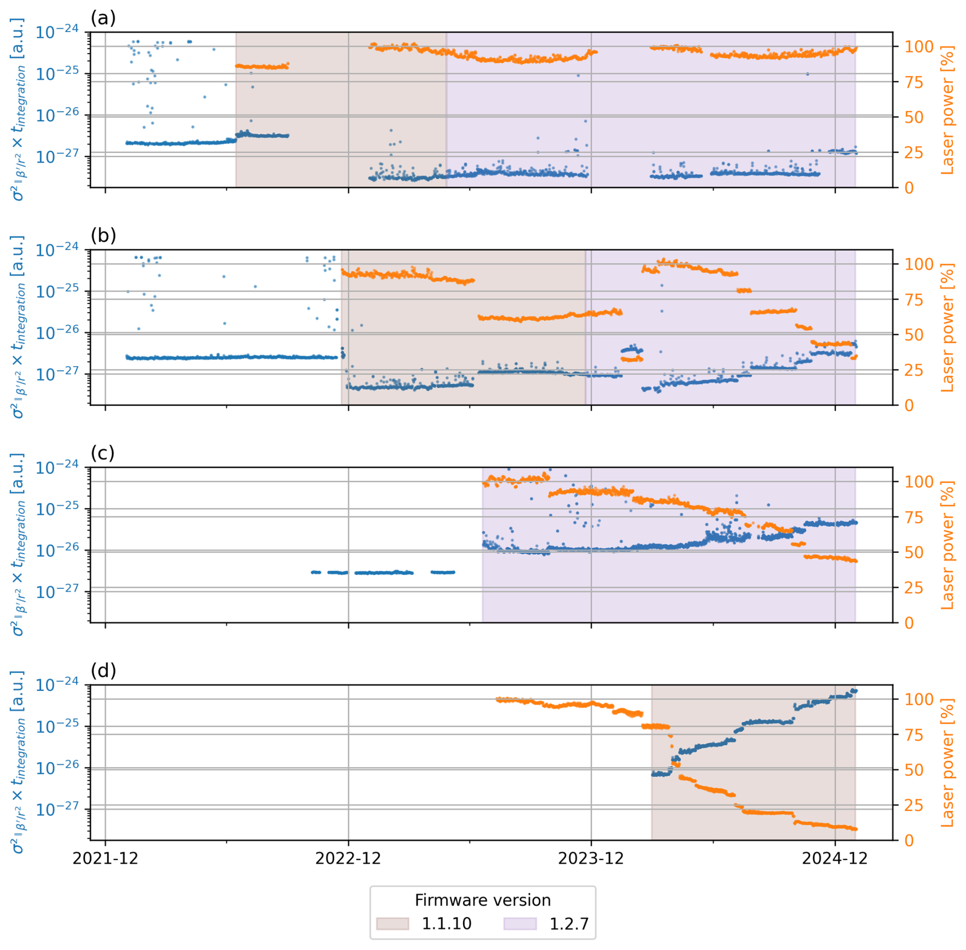
Figure 4 Time series of nighttime background signal variance normalized by the integration time (${\mathit{\sigma }}_{{}^{\parallel }{\mathit{\beta }}^{\prime }/r^{\mathrm{2}}}^{\mathrm{2}}\times t_{\mathrm{intergration}}$), and the laser power are shown for (a) Vehmasmäki, (b) Hyytiälä, (c) Kenttärova, and (d) Lindenberg. Shaded regions denote different firmware versions; unshaded areas represent periods with no recorded firmware version and laser power.

At Hyytiälä and Kenttärova, laser power gradually decreases from 100 % to around 40 % over 2 years. In contrast, the CL61 at Vehmasmäki maintains a consistently high laser power, ranging between 90 % and 100 % throughout the same period, with only a slight decrease during the summer, likely to regulate the internal temperature to prevent overheating. Meanwhile, the CL61 at Lindenberg experienced a sharp decline in laser power, from 80 % to below 10 % within just 1 year of operation. We also found that changes in the firmware version do not appear to have any noticeable effect on background noise levels.

The relationship between background noise, normalized by integration time, and laser power across several instruments is illustrated in Fig. 5. Nighttime measurements (23:00 to 01:00 local time; LT), shown in blue, are unaffected by solar radiation, while all-day measurements are displayed in grey. It is important to note that the selected nighttime window is arbitrary and used solely for this analysis; for instance, locations such as Kenttärova experience no true nighttime during summer. The nighttime data clearly indicate that a decrease in laser power leads to an increase in background noise across all instruments. Daytime background noise is generally higher due to solar radiation, which varies with factors such as solar angle, cloud height, and surface albedo, making direct comparisons more complex. Nevertheless, the figure suggests that lower laser power also contributes to increased noise levels during daytime conditions.

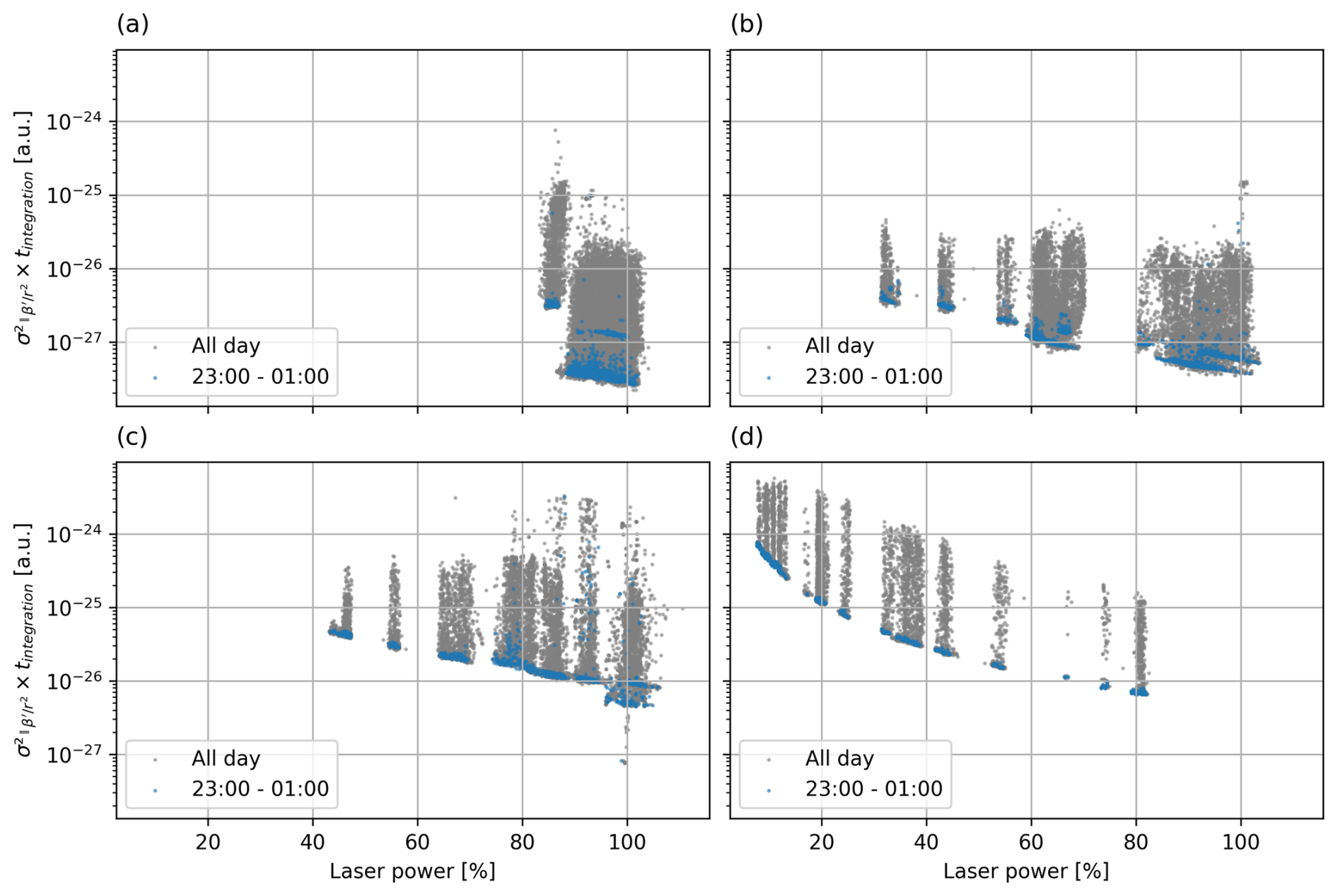
Figure 5 Variance of background noise as a function of laser power percentage, normalized by integration time, at the following locations: (a) Vehmasmäki, (b) Hyytiälä, (c) Kenttärova, and (d) Lindenberg. Blue points represent data collected during nighttime hours (23:00–01:00 LT), while grey points include all available data.

An increase in background noise can significantly reduce an instrument's ability to detect weak aerosol signals. This effect is clearly illustrated in Fig. S3. On 7 March 2024, an elevated aerosol layer was observed above 3 km in Lindenberg, indicated by enhanced attenuated backscatter coefficient values compared to those at lower altitudes between 1 and 3 km (Fig. S3a, c). However, by 2 December 2024, a reduction in laser power led to a higher noise floor, which meant that if a similar aerosol layer were present, it would no longer be distinguishable from the background noise (Fig. S3b, c).

4.2 Instrumental background

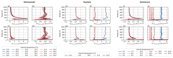
In this section, we examine how the instrumental background bias (${\mathit{\mu }}_{P_{\mathrm{instrument}}O\left(r\right)}$) and noise (${\mathit{\sigma }}_{P_{\mathrm{instrument}}O\left(r\right)}^{\mathrm{2}}$) with the overlap correction reverted, vary with temperature and over time. The termination hood measurement was deployed multiple times at Vehmasmäki, Hyytiälä, and Kenttärova. Figure 6 presents the instrumental background profiles recorded during these termination hood measurement periods, which have been averaged and grouped according to the instruments' internal temperatures.

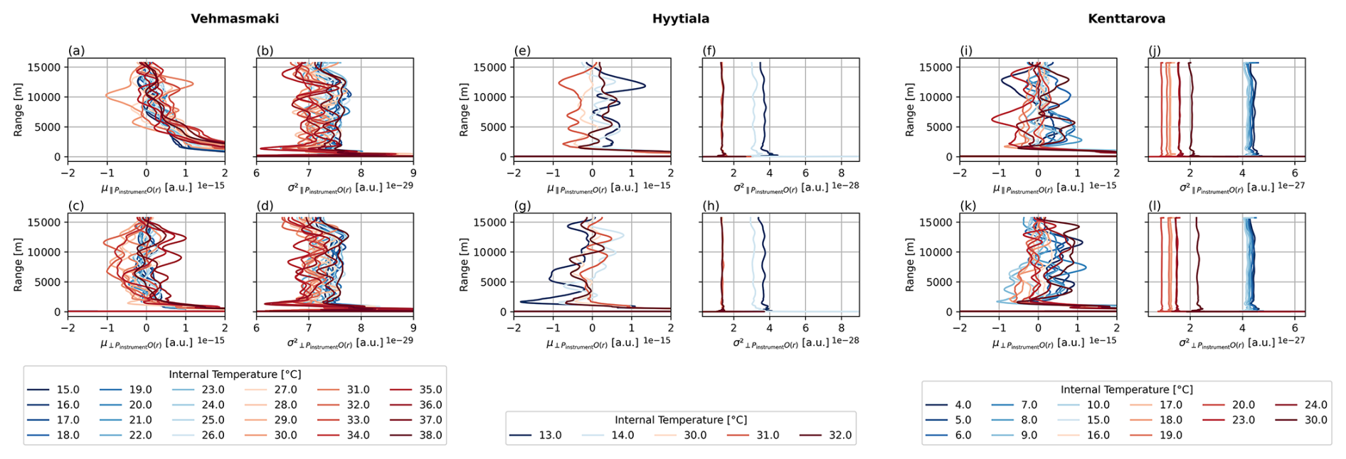
Figure 6 Termination hood profiles at various internal temperatures (color-coded) across different sites. In Vehmasmäki: (a) ${\mathit{\mu }}_{{}^{\parallel }{P}_{\mathrm{instrument}}O\left(r\right)}$, (b) ${\mathit{\sigma }}_{{}^{\parallel }{P}_{\mathrm{instrument}}O\left(r\right)}^{\mathrm{2}}$, (c) ${\mathit{\mu }}_{{}^{⟂}{P}_{\mathrm{instrument}}O\left(r\right)}$, and (d) ${\mathit{\sigma }}_{{}^{⟂}{P}_{\mathrm{instrument}}O\left(r\right)}^{\mathrm{2}}$. In Hyytiälä: (e) ${\mathit{\mu }}_{{}^{\parallel }{P}_{\mathrm{instrument}}O\left(r\right)}$, (f) ${\mathit{\sigma }}_{{}^{\parallel }{P}_{\mathrm{instrument}}O\left(r\right)}^{\mathrm{2}}$, (g) ${\mathit{\mu }}_{{}^{⟂}{P}_{\mathrm{instrument}}O\left(r\right)}$, and (h) ${\mathit{\sigma }}_{{}^{⟂}{P}_{\mathrm{instrument}}O\left(r\right)}^{\mathrm{2}}$. In Kenttärova: (i) ${\mathit{\mu }}_{{}^{\parallel }{P}_{\mathrm{instrument}}O\left(r\right)}$, (j) ${\mathit{\sigma }}_{{}^{\parallel }{P}_{\mathrm{instrument}}O\left(r\right)}^{\mathrm{2}}$, (k) ${\mathit{\mu }}_{{}^{⟂}{P}_{\mathrm{instrument}}O\left(r\right)}$, and (l) ${\mathit{\sigma }}_{{}^{⟂}{P}_{\mathrm{instrument}}O\left(r\right)}^{\mathrm{2}}$.

For the instruments located in Hyytiälä and Kenttärova, the ${\mathit{\mu }}_{{}^{\parallel }{P}_{\mathrm{instrument}}O\left(r\right)}$ profiles remain relatively stable around zero from the far range down to about 2 km, then increase sharply as the range decreases. On the other hand, in Vehmasmäki, it also remains near zero at far range, but ${\mathit{\mu }}_{{}^{\parallel }{P}_{\mathrm{instrument}}O\left(r\right)}$ begins to increase already at around 5 km and continues to rise toward shorter ranges. Meanwhile, the ${\mathit{\mu }}_{{}^{⟂}{P}_{\mathrm{instrument}}O\left(r\right)}$ profiles for all three instruments remain near zero from the far range to about 2 km, after which they increase rapidly with decreasing range.

Overall, the internal temperature T has a more pronounced effect on the ${\mathit{\mu }}_{P_{\mathrm{instrument}}O\left(r\right)}$ profiles below 1 km than at higher ranges. In particular, the ${\mathit{\mu }}_{P_{\mathrm{instrument}}O\left(r\right)}$ profiles in both polarizations deviate substantially from zero at below 200 m (see Fig. 7) across all instruments. Notably, each instrument shows the same small peak in the instrumental background bias in both polarizations at approximately 150 m.

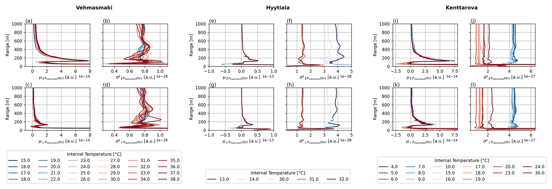
Figure 7 Termination hood profiles at various internal temperatures (color-coded) across different sites only up to 1000 m range. In Vehmasmäki: (a) ${\mathit{\mu }}_{{}^{\parallel }{P}_{\mathrm{instrument}}O\left(r\right)}$, (b) ${\mathit{\sigma }}_{{}^{\parallel }{P}_{\mathrm{instrument}}O\left(r\right)}^{\mathrm{2}}$, (c) ${\mathit{\mu }}_{{}^{⟂}{P}_{\mathrm{instrument}}O\left(r\right)}$, and (d) ${\mathit{\sigma }}_{{}^{⟂}{P}_{\mathrm{instrument}}O\left(r\right)}^{\mathrm{2}}$. In Hyytiälä: (e) ${\mathit{\mu }}_{{}^{\parallel }{P}_{\mathrm{instrument}}O\left(r\right)}$, (f) ${\mathit{\sigma }}_{{}^{\parallel }{P}_{\mathrm{instrument}}O\left(r\right)}^{\mathrm{2}}$, (g) ${\mathit{\mu }}_{{}^{⟂}{P}_{\mathrm{instrument}}O\left(r\right)}$, and (h) ${\mathit{\sigma }}_{{}^{⟂}{P}_{\mathrm{instrument}}O\left(r\right)}^{\mathrm{2}}$. In Kenttärova: (i) ${\mathit{\mu }}_{{}^{\parallel }{P}_{\mathrm{instrument}}O\left(r\right)}$, (j) ${\mathit{\sigma }}_{{}^{\parallel }{P}_{\mathrm{instrument}}O\left(r\right)}^{\mathrm{2}}$, (k) ${\mathit{\mu }}_{{}^{⟂}{P}_{\mathrm{instrument}}O\left(r\right)}$, and (l) ${\mathit{\sigma }}_{{}^{⟂}{P}_{\mathrm{instrument}}O\left(r\right)}^{\mathrm{2}}$.

All instruments exhibit profiles of ${\mathit{\sigma }}_{P_{\mathrm{instrument}}O\left(r\right)}^{\mathrm{2}}$ in both polarizations that remain constant above 500 m, followed by a sharp increase below this range. These instrumental background noise profiles show a pronounced sensitivity to internal temperature (from 4 to 38 °C). Notably, very low temperatures are associated with elevated instrumental background noise across the entire measurement range. This can be explained by the effect of the internal heater. As the internal temperature falls below an instrument-specific threshold (15 °C for Hyytiälä and Kenttärova), the internal heater is turned on. This leads to an increase in ${\mathit{\sigma }}_{P_{\mathrm{instrument}}O\left(r\right)}^{\mathrm{2}}$, with the effect becoming more pronounced as the temperature decreases. When the internal temperature is high and the internal heater is off, internal temperature positively correlates with ${\mathit{\sigma }}_{P_{\mathrm{instrument}}O\left(r\right)}^{\mathrm{2}}$.

Similar to Figs. 6, 7, S4 and S5 show the same profiles obtained during the termination hood measurements, but include range correction and the instrument-provided overlap correction. These profiles of ${}^{\parallel }{\mathit{\beta }}^{\prime }$ and ${}^{⟂}{\mathit{\beta }}^{\prime }$ provide a direct quantification of the impact of instrumental background bias and noise on the measurements and their dependence on temperature. For all CL61 instruments, the instrumental biases, ${\mathit{\mu }}_{{}^{\parallel }{\mathit{\beta }}^{\prime }}$ and ${\mathit{\mu }}_{{}^{⟂}{\mathit{\beta }}^{\prime }}$, remain below the order of 10⁻⁷, while the noise terms, ${\mathit{\sigma }}_{{}^{\parallel }{\mathit{\beta }}^{\prime }}^{\mathrm{2}}$ and ${\mathit{\sigma }}_{{}^{⟂}{\mathit{\beta }}^{\prime }}^{\mathrm{2}}$, remain below the order of 10⁻¹¹. These biases are even smaller below 5 km. Below a range of 1 km, ${\mathit{\mu }}_{{}^{\parallel }{\mathit{\beta }}^{\prime }}$ remains below 5 × 10⁻⁹ and ${\mathit{\mu }}_{{}^{⟂}{\mathit{\beta }}^{\prime }}$ below 3 × 10⁻⁹. These small biases are usually negligible comparing to the typical atmospheric signal.

However, at very clean sites such as Kenttärova, the instrumental bias in ${}^{⟂}{\mathit{\beta }}^{\prime }$ can still affect the retrieved aerosol depolarization ratio, particularly under conditions of low depolarization. An example is shown in Fig. S6, which presents measurements from Kenttärova on 3 October 2023 under weakly depolarizing aerosol conditions. During this period, the ${}^{⟂}{\mathit{\beta }}^{\prime }$ profile below 400 m is on the order of 10⁻⁹, while ${}^{\parallel }{\mathit{\beta }}^{\prime }$ remains on the order of 10⁻⁶. As a result, the instrumental bias becomes relatively significant for ${}^{⟂}{\mathit{\beta }}^{\prime }$, leading to a noticeable, although quantitatively small, reduction in δ (from 0.002 to 0.001 at 200 m) after the bias correction is applied. Furthermore, the previously mentioned peak at 150 m is clearly visible in this case and is effectively mitigated after the removal of the instrumental bias. Overall, the impact of the bias correction is expected to be most pronounced under clean atmospheric conditions, such as in this case in Finland, where the δ profile remains consistently low. The correction improves the overall shape of the profile, particularly around 150 m, by removing the artificial peak in ${}^{⟂}{\mathit{\beta }}^{\prime }$ at that height (Fig. S6). However, the change remains small in absolute terms.

For all instruments, the signal near the surface exhibits much more rapid fluctuations than at higher range gates. Figure S7 displays example profiles of ${}^{\parallel }{\mathit{\beta }}^{\prime }$, ${}^{⟂}{\mathit{\beta }}^{\prime }$, and the instrument's internal temperature during a termination hood measurement at Kenttärova, revealing periodic variations in the signal below 50 m. To investigate this, the Fourier transforms of these signals were computed at each range gate over time and compared to that of the laser temperature recorded simultaneously. The results show that both the signals and the laser temperature exhibit a coincident spectral peak at approximately 0.0079 Hz (about 120 s), indicating a strong influence of laser temperature on the signals. Furthermore, additional distinct peaks in the signal spectra imply the presence of other instrument-related effects. Overall, these periodic variations appear sporadically across all instruments, with no consistent pattern indicating when they appear or disappear. Given the difficulty in developing a reliable correction method, we recommend excluding measurements below 50 m.

Figure 8 shows how the instrumental bias during the termination hood measurement at Vehmasmäki varies over time under consistent internal temperature conditions. Over a 6-month period, the calibration profiles at each temperature show only minor fluctuations. Therefore, we recommend performing termination hood checks at least once across the operating temperature range to determine the instrumental background bias and noise.

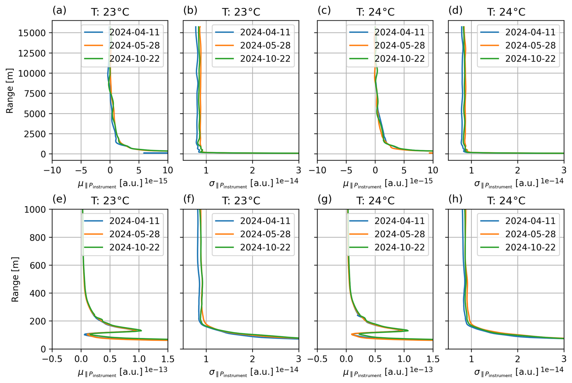
Figure 8 Termination hood profiles in Vehmasmäki at (a, b, e, f) 23 °C, and (c, d, g, h) 24 °C. These measurements were recorded at three different time points over a 6-month period in 2024. Panels (a), (c), (e), and (g) display ${\mathit{\mu }}_{{}^{\parallel }{\mathit{\beta }}^{\prime }}$, while panels (b), (d), (f), and (h) display ${\mathit{\sigma }}_{{}^{\parallel }{\mathit{\beta }}^{\prime }}$.

4.3 Calibration

Figure 9 presents the time series of calibration factor from the cloud calibration and Rayleigh calibration methods for all the ceilometers. Detailed results of the cloud calibration factors derived from liquid cloud signals at each site are presented in Figs. S8–S11. Overall, the calibration factors obtained from the two methods agree well within their respective uncertainties, In Lindenberg, the calibration factor from the cloud calibration exhibits an approximate threefold decline over time, reflecting notable signal degradation. During this degradation period, Rayleigh calibration could not be performed because the elevated background-noise level (see Sect. 4.1) obscured the molecular return. In contrast, the other instruments show only short-term fluctuations without any clear long-term trend. Two periods with notable deviations in the calibration factor were also identified: June to October 2023 and November to December 2024 in Vehmasmäki. The issue in the CL61 at Vehmasmäki is due to the fogged window that attenuates the outgoing signal. This will be analyzed in more detail in the following section.

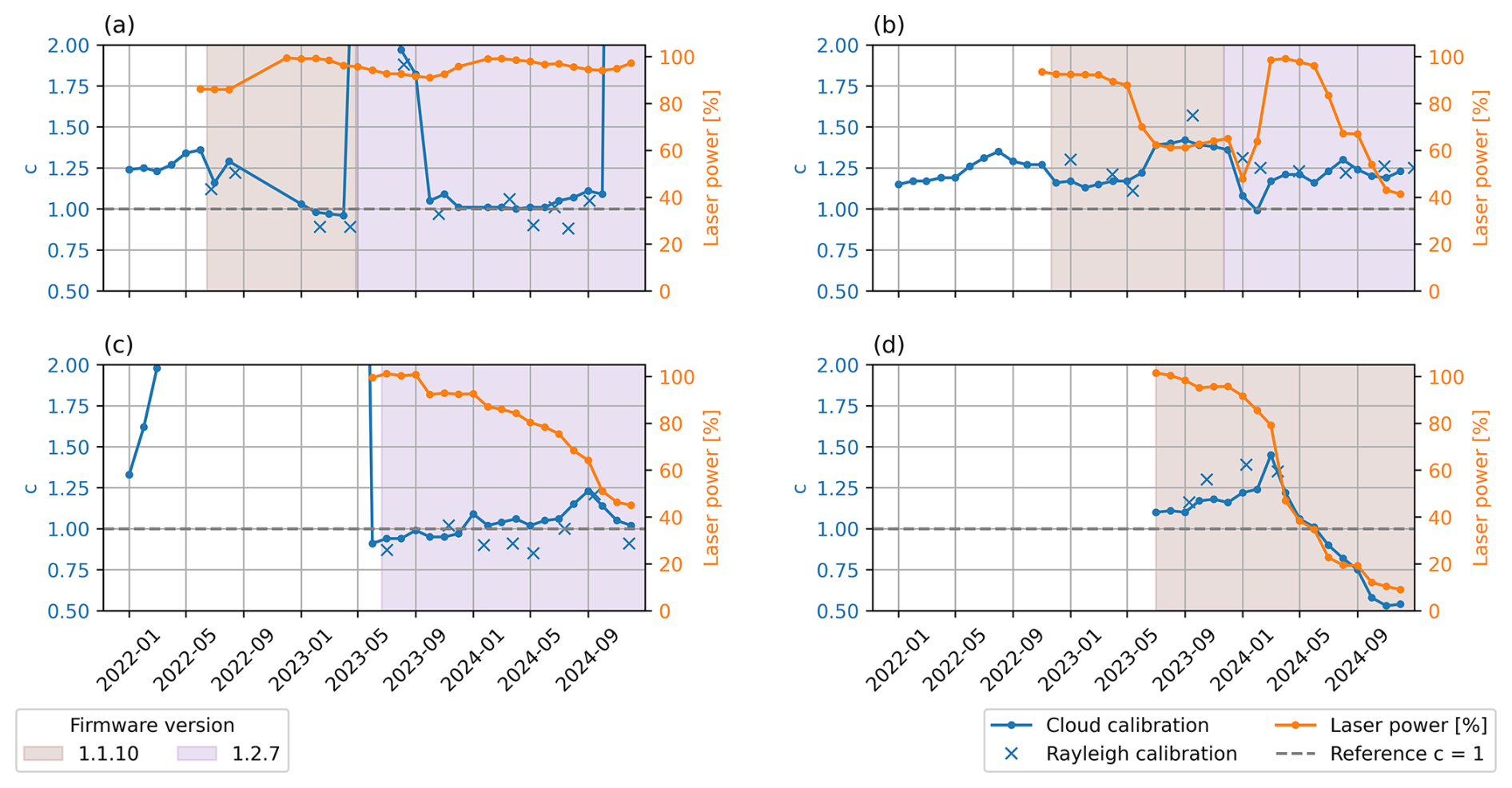
Figure 9 Time series of the calibration factor from cloud calibration, Rayleigh calibration and laser power at four sites: (a) Vehmasmäki, (b) Hyytiälä, (c) Kenttärova, and (d) Lindenberg. The dashed line indicates a calibration factor of c = 1. Periods corresponding to different firmware versions are highlighted with shaded areas.

Across all instruments, the calibration factor generally stays within the range of 0.9 to 1.5 as long as laser power remains above 40 %, aside from occasional deviations due to specific instrument issues. In Vehmasmäki, as the laser power remains above 90 %, the calibration factor fluctuates around 1 within 10 % fluctuation. In Hyytiälä, the highest changes in calibration factor is observed when the instrument's laser power is below 80 % with the firmware 1.1.10 and then below 60 % with the firmware 1.2.7. However, the calibration factor remains relatively stable at 1.25 even when the laser power drops from 100 % to 40 % with the firmware 1.2.7. In Kenttärova, laser power percentages were not recorded before June 2023, but the observed increase in the calibration factor is likely linked to a decrease in laser power. After a new transmitter was installed, the calibration factor returned to around 1. In Lindenberg, a noticeable decline in the cloud calibration factor was observed as laser power dropped from 40 % to 10 %. It is still to be ascertained whether this trend also appears in instruments running the newer firmware version 1.2.7.

Figure S12 demonstrates the utility of cloud calibration for two cases; one with 80 % laser power on 3 March 2024 and another with just 10 % on 16 November 2024. This indicates that the method can still be used in situations with low laser power. Since the internal calibration value may not scale with low laser power values, regular cloud calibration is necessary to understand instrument performance and continue to provide profiles that can be used quantitatively, especially for laser power values below 40 %.

4.4 Signal correction and uncertainty estimation

After recording the termination hood profiles at different temperatures and determining the calibration factor, the correction and forward Klett inversion can be applied, and the associated uncertainty can be estimated using the method described in Sect. 3.3. Example results of this procedure are illustrated in Figs. 10 and 11 showcasing a typical Finnish low aerosol load condition in Kenttärova. During this period, the calibration factor was close to 1. On this date (Fig. 11), aerosol was present below 1000 m within the boundary layer close to the ground, while several layers of clouds extended from 2 up to 3.5 km. Figure 10 presents the β, δ and their associated uncertainties in the aerosol layer below 1000 m obtained from a measurement profile recorded at 13:01 UTC on the same day.

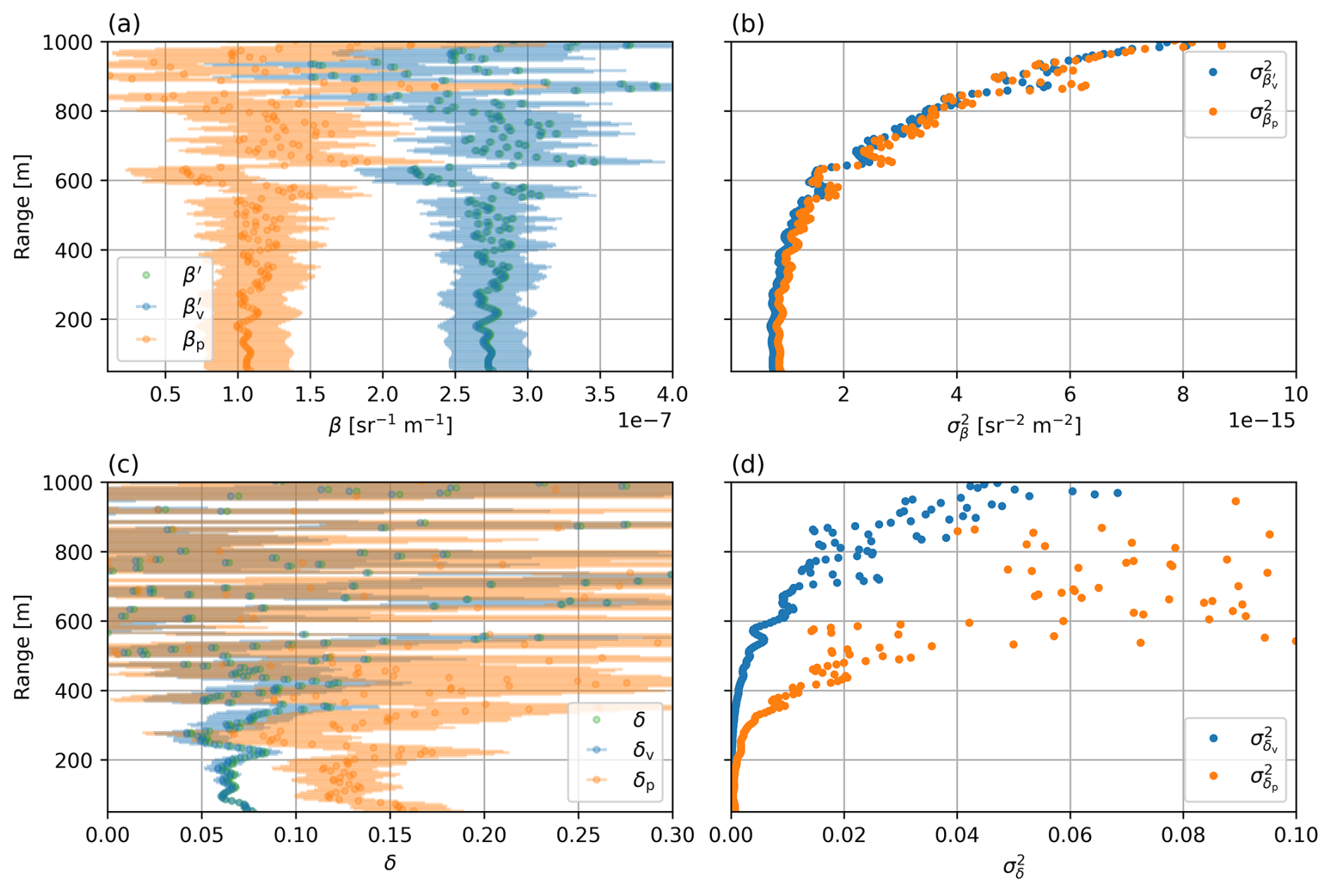
Figure 10 Example of uncorrected and corrected profiles in Kenttärova measured on 4 June 2024 at 13:01 UTC. (a) β^′ (instrument provided), ${\mathit{\beta }}_{\mathrm{v}}^{\prime }$ (bias corrected and calibrated), β_p, (b) ${\mathit{\sigma }}_{{\mathit{\beta }}_{\mathrm{v}}^{\prime }}^{\mathrm{2}}$, ${\mathit{\sigma }}_{{\mathit{\beta }}_{\mathrm{p}}}^{\mathrm{2}}$, (c) δ (instrument provided), δ_v (bias corrected and calibrated), δ_p, (d) ${\mathit{\sigma }}_{{\mathit{\delta }}_{\mathrm{v}}}^{\mathrm{2}}$, ${\mathit{\sigma }}_{{\mathit{\delta }}_{\mathrm{p}}}^{\mathrm{2}}$. Error bars represent 1 standard deviation (σ) of the measurements.

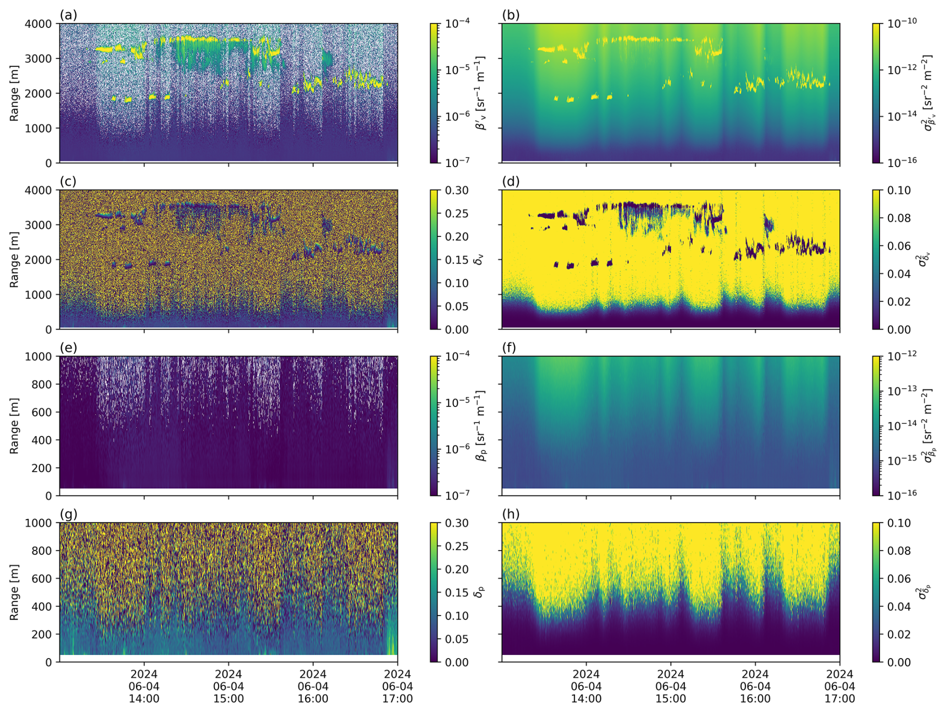
Figure 11 An example of corrected and calibrated profile in Kenttärova on 4 June 2024 at 13:00–17:00 UTC (same day as Fig. 10). (a) ${\mathit{\beta }}_{\mathrm{v}}^{\prime }$, (b) ${\mathit{\sigma }}_{{\mathit{\beta }}_{\mathrm{v}}^{\prime }}^{\mathrm{2}}$ (c) δ_v, (d) ${\mathit{\sigma }}_{{\mathit{\delta }}_{\mathrm{v}}}^{\mathrm{2}}$ (e) β_p, (f) ${\mathit{\sigma }}_{{\mathit{\beta }}_{\mathrm{p}}}^{\mathrm{2}}$, (g) δ_p, and (h) ${\mathit{\sigma }}_{{\mathit{\delta }}_{\mathrm{p}}}^{\mathrm{2}}$. For particle properties in panels (e)–(h), profiles are shown only up to 1 km range.

At below 1000 m range, the corrected ${\mathit{\beta }}_{\mathrm{v}}^{\prime }$ differs only slightly from the original uncorrected β^′, with the difference ranging from 1 × 10⁻⁹ to 2.5 × 10⁻⁹ sr⁻¹ m⁻¹ (Fig. 10a). This difference is expected to be relatively smaller within the clouds, where the signal is stronger and the instrumental bias decreases with increasing range. In contrast, the particle backscatter coefficient β_p is substantially lower than ${\mathit{\beta }}_{\mathrm{v}}^{\prime }$ by approximately 1.5 × 10⁻⁷ sr⁻¹ m⁻¹, indicating a significant contribution from molecular scattering. The ${\mathit{\sigma }}_{{\mathit{\beta }}_{\mathrm{v}}^{\prime }}^{\mathrm{2}}$ and ${\mathit{\sigma }}_{{\mathit{\beta }}_{\mathrm{p}}}^{\mathrm{2}}$ profiles are relatively similar to each other, and they both increase exponentially with height (Fig. 10b).

Similarly, the original uncorrected (δ) and the corrected (δ_v) profiles differ only slightly, by the difference is about 0.001 to 0.005 (Fig. 10c) while δ itself being around 0.07. In contrast, the particle linear depolarization ratio δ_p is substantially higher, differing from the original δ by approximately 0.1 with δ_p at around 0.1 to 0.15. For example, during pollen seasons in Finland, δ_p has been observed at 0.23 for pine and 0.26 for birch at this wavelength (Filioglou et al., 2023). The variances (${\mathit{\sigma }}_{{\mathit{\delta }}_{\mathrm{v}}}^{\mathrm{2}}$, ${\mathit{\sigma }}_{{\mathit{\delta }}_{\mathrm{p}}}^{\mathrm{2}}$) are comparable below 200 m, but at higher ranges, ${\mathit{\sigma }}_{{\mathit{\delta }}_{\mathrm{p}}}^{\mathrm{2}}$ becomes markedly larger.

Overall, the pronounced differences between ${\mathit{\beta }}_{\mathrm{v}}^{\prime }$ and β_p, as well as between δ_v and δ_p, highlight the importance of accounting for the molecular contribution when performing quantitative assessments of aerosol measurement with CL61 for low aerosol load conditions in Finland. While the difference between β^′ and ${\mathit{\beta }}_{\mathrm{v}}^{\prime }$ (and δ and δ_v) may be small, the termination hood remains important as it allows the estimation of measurement uncertainties. Averaging multiple profiles reduces the uncertainties, as illustrated in Fig. S13, which shows the profiles averaged over 10 min.

Figure 11 illustrates the time series of ${\mathit{\beta }}_{\mathrm{v}}^{\prime }$, δ_v, β_p, and δ_p profiles, along with their corresponding variances on the same day. Similar to Fig. 10, ${\mathit{\beta }}_{\mathrm{v}}^{\prime }$ is higher than β_p, while δ_v is lower than δ_p in this period. The profiles of ${\mathit{\sigma }}_{{\mathit{\beta }}_{\mathrm{v}}^{\prime }}^{\mathrm{2}}$ and ${\mathit{\sigma }}_{{\mathit{\beta }}_{\mathrm{p}}}^{\mathrm{2}}$ vary with time during this period, exhibiting an exponential increase with range. On the other hand, the ${\mathit{\sigma }}_{{\mathit{\delta }}_{\mathrm{v}}}^{\mathrm{2}}$ and ${\mathit{\sigma }}_{{\mathit{\delta }}_{\mathrm{p}}}^{\mathrm{2}}$ profiles demonstrate a more pronounced dependence on the signal magnitude (Fig. 11d and h), with stronger atmospheric signals resulting in smaller uncertainties.

4.5 Signal loss

As previously noted, abrupt changes in the cloud calibration factor at Vehmasmäki were observed from June to October 2023 and again from November to December 2024. Similar deviations are present during the same periods, as seen in the window condition housekeeping variable (Fig. S14). These patterns indicate that an obstruction, likely on the instrument window, was attenuating both outgoing and incoming laser beams.

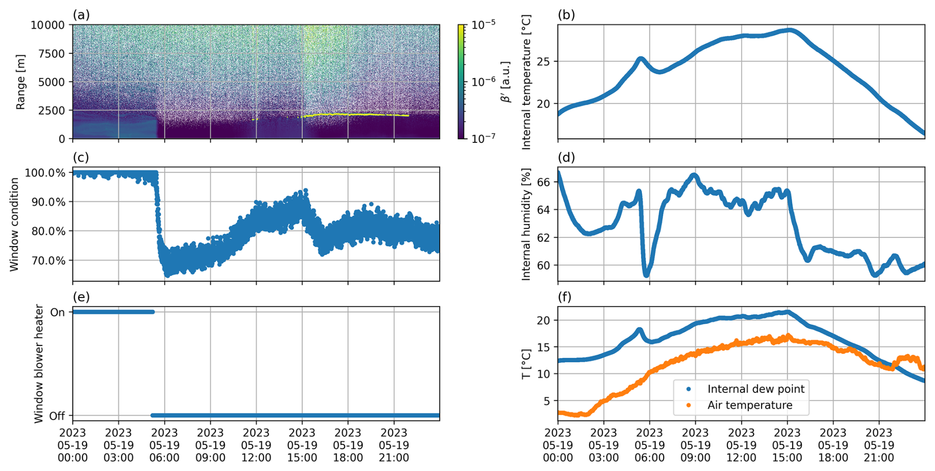
Figure 12 Measurements from Vehmasmäki on 19 May 2023: (a) β^′, (b) internal temperature, (c) window condition, (d) internal humidity, (e) window blower heater, and (f) calculated dew point and measured outside air temperature.

Figure 12 illustrates a specific example from 19 May 2023. On this date, a sudden drop in the attenuated backscatter signal below 2000 m occurred just before 06:00 UTC. At the same time, the window condition value sharply declined from around 100 % to 70 %. This coincided with the automatic deactivation of the window blower heater. Housekeeping data, including internal temperature and relative humidity, were used to estimate the internal dew point, which was then compared to the external air temperature. When the window blower heater was off, the window cooled to match the outside air temperature. Once the window temperature dropped below the internal dew point, condensation began to form on the inside surface of the window and attenuated the signal. This occurred despite the measured internal relative humidity remaining below 70 %. This is because the measurement does not represent the relative humidity at the window surface, where the temperature is closer to ambient temperature.

Since condensation affects the entire signal profile and the degree of attenuation depends on its severity, it is not possible to precisely quantify the signal loss or reconstruct the original profile. This issue could be mitigated by keeping both the window blower and heater always on. However, at the time of this writing, this is not possible (personal communication with Vaisala). Additionally, hardware modifications may be required to maintain a sufficiently low internal dew point and prevent fogging.

5 Conclusions

In this study, we investigate several characteristics of CL61 measurements across multiple sites over a 3-year period, using methodologies adapted from existing approaches.

First, we examine the temporal evolution of the background noise and its relationship with laser power. The background noise generally increases as the laser power decreases, which is particularly important because laser aging can substantially reduce the CL61's capability to detect weak aerosol signals. For most instruments, internal scaling of the calibration factor effectively compensates for changes in laser power. However, for the instrument at the Lindenberg site with an older firmware version (1.1.10), this compensation becomes insufficient when laser power drops below 40 %, resulting in a drift in the calibration factor. Therefore, regular cloud calibration is necessary to ensure quantitatively reliable profiles, especially when the laser power falls below 40 %. Additionally, some deviations in the calibration factor were linked to the fogging of the inside surface of the window.

Second, we performed termination hood measurements to characterize the instrumental residual background bias and noise profiles. The magnitude of the residual background bias for all instruments is generally small. In a case study in Kenttärova, the magnitude of the residual bias was approximately 1 %–2 % of the molecular backscatter. Nevertheless, the termination hood measurements remain crucial, as they allow the instrumental background to be quantified and subsequently used to estimate the uncertainties of the particle backscatter coefficient (β_p) and the particle linear depolarization ratio (δ_p), as presented in this study.

Third, we found that the instrumental residual background bias and noise profiles are sensitive to temperature and exhibit differences between parallel and perpendicular polarizations. We also recommend discarding the first 50 m of measurements, where periodic variations were frequently observed. Instrumental background profiles were obtained across a range of internal temperatures and were subsequently used to correct the bias and estimate its associated uncertainty. These profiles remained stable for at least one month for a given internal temperature, although small deviations appeared over a 6-month period. Consequently, we recommend making termination hood measurements at least once across the operating temperature range to characterize the instrumental background.

Fourth, we demonstrate that the molecular contribution to the measured depolarization ratio can be substantial, reaching approximately 0.1, whereas the impact of residual background bias is only around 0.005 in the same case study. This highlights the importance of accounting for the molecular contribution in CL61 depolarization ratio measurement under low aerosol load conditions.

Finally, we identify window fogging as an important issue affecting CL61 data quality. Fogging of the inside surface of the window was observed in some instruments and resulted in degraded measurements. Identifying and excluding such periods is therefore essential for ensuring the integrity of the dataset and the reliability of subsequent analyses.