Improving multi-modal wind speed prediction of short and medium term with a bi-clustered machine learning method

Accurate prediction of wind speed is of great importance for stable and reliable operation of wind farms. However, the single numerical model forecast cannot provide precise wind speed outputs due to the defect of its physical parameterization scheme, whose error will gradually grow with increasing prediction time. Therefore, we proposed a model named Bi-clustered Recursive Bayesian Forest (BCRBR) for wind speed prediction and correction. The approach incorporated Sea-land Breeze and weather stability effects, integrating an atmospheric circulation index as input features; wind farm data underwent modal classification via bi-clustering to mitigate wind speed magnitude interactions, followed by machine learning-based correction of wind speed. The method was proved to be effective for wind speed prediction correction. Compared to forecasts from the Weather Research and Forecasting model, wind speed error indicators were reduced by more than 60 %; and the forecast precision increased from 30.2 % to 78.4 %, of which the improvement is more than twice. Compared to other models, the proposed model presented favorable correction results in different types of wind field, indicating its greater versatility and stronger competitiveness than other models.

1 Introduction

The demand for renewable energy is increasing globally due to the depletion of non-renewable fossil fuels and the deterioration of the ecological environment, leading to a gradual shift towards new energy as the primary power source. In 2024, the global newly installed capacity of wind power reached a record high of 117 GW, with the cumulative installed capacity reaching 1136 GW, an increase of 11 % compared to 2023 (Global Wind Energy Council, 2025). The increasing need for wind power is a positive sign for the energy transition in line with the goals of carbon neutrality. Offshore wind farms can generate more energy compared to onshore wind farms. As a crucial source of clean energy, its consistent and reliable operation enables better integration of a large volume of wind energy, thereby improving the stability of the power system and improving the efficiency of the generation (Enevoldsen and Valentine, 2016). Wind speed usually has a close and complex relationship with the output power of wind power generation, and wind speed prediction errors will be directly transferred to the wind power prediction (Liu et al., 2020). The power output of the wind farm shows significant variability and uncertainty due to the complex oceanic meteorological conditions, the atmospheric laminar flow, and other factors influencing the speed of the wind (Xiong et al., 2023; Zheng et al., 2016). Rapid fluctuation of wind power can disrupt the balance of supply, demand, and safe operation of the power system. In extreme weather conditions, it can even lead to widespread blackouts and the collapse of the power grid, resulting in significant economic losses to society (Khazaei et al., 2022; Yildiz et al., 2021; Xu et al., 2022; Demolli et al., 2019). Therefore, precise forecasting of wind speed is imperative for the achievement of renewable energy development objectives.

Based on the fundamental principles and operational mechanisms of the model, current wind speed prediction methods can be broadly categorized into two groups: physical approaches and statistical techniques (Wang et al., 2022; He et al., 2018). Numerical Weather Prediction (NWP), a physical approach, utilizes computer models to simulate the evolution of atmospheric systems for weather forecasting. It is capable of simulating large-scale meteorological processes, including the progression of wind speed, making it particularly suitable for long-term prediction of wind speed in the context of wind farms (Zhao et al., 2018; Son and Jung, 2021; Brotzge et al., 2023). Common NWP models include the high-resolution limited area model (HIRLAM) (Landberg, 1999), Mesoscale Model5 (MM5) (Salcedo-Sanz et al., 2011), European Centre for Medium-Range Weather Forecasts (ECMWF), and Weather Research and Forecasting model (WRF) (Prósper et al., 2019). Currently, the main method for predicting future wind speeds in the field of wind power prediction is the use of the WRF model (Zhou et al., 2023). However, due to factors such as the imperfection of physical parameterization schemes, low resolution, inaccurate terrain, and others, significant errors exist in numerical weather prediction. The process of atmospheric motion is the result of the joint effect of historical and current states. As the duration of the prediction increases, the NWP wind speed prediction error, which is the main input of the intelligent learning model, will accumulate over time, thereby leading to a notable decline in the accuracy of the wind power prediction model. Additionally, the considerable amount of computing time makes it unsuitable for short-term predictions (Zhao et al., 2019; Xu et al., 2021).

Statistical methods encompass both traditional statistical models and machine learning models, typically developed using a large volume of historical monitoring data and meteorological synchronous observation data. They serve as a crucial complement to numerical model approaches (Katinas et al., 2018; Ouarda and Charron, 2021). Traditional statistical models (e.g., time series, regression) do not simulate atmospheric physics; they are computationally efficient but lack nonlinear fitting ability, leading to lower prediction accuracy (Yousuf et al., 2022). In contrast, machine learning models learn from historical data without strict physical assumptions, effectively capturing complex nonlinear relationships and achieving higher accuracy. They also generalize well with large datasets. However, ML models are data-dependent and require extensive training and tuning (Ley et al., 2022). The typical range of RMSE for WRF offshore wind speed forecasts is currently 1.5–3.5 m s⁻¹, and the error patterns are related to sea-land breezes and atmospheric stability – precisely the kind of nonlinear mapping that machine learning can capture (Gong et al., 2025; Kang et al., 2020). Since it is difficult to completely eliminate these errors by simply improving the WRF physical model or data assimilation, recent studies have begun to use machine learning methods to post-process and correct WRF outputs (Salvão et al., 2025; Tsai et al., 2021; Zhou and He, 2017).

With the development of research for a long time, the accuracy of any single prediction method is almost saturated. Therefore, in practical engineering applications, the single model should be supplemented with other methods to achieve high-precision wind power prediction. Parri and Teeparthi (Parri and Teeparthi, 2024) introduced a hybrid wind speed prediction model (SVMD-TF-QS) that integrates a novel query selection mechanism (QS), continuous variational mode decomposition (SVMD), and a Transformer (TF)-based model to accurately forecast wind speed while minimizing computational load. Zheng and Wang (2024) combined several algorithms based on recurrent neural networks and used the Levy crystal structure algorithm for weight optimization to create a short-term wind speed prediction model. These hybrid models effectively leveraged the strengths of individual models to improve forecast accuracy and reliability. Prediction models based on multi-algorithm fusion will become an important development direction in the field of wind speed prediction.

In offshore wind farms, wind speed is influenced by complex meteorological processes, among which sea-land breeze (SLB) plays a critical role due to diurnal temperature contrasts (Shen, 2021). SLB modulates turbulence intensity and wind speed gradients, potentially altering wind-power characteristics.However, to date, few studies have considered the impacts of weather systems, terrain, and day-night alternation on wind speed. In summary, the following problems remain to be solved in the field of wind speed prediction:

1. The feature factors input to the corrected model for wind speed prediction have significant limitations. Traditional forecast revision models use historical wind speed data as input and have not considered the interactions between meteorological factors. It does not have any feature selection and lacks feature quantities that can indicate the trend of weather stability;

2. The factors influencing the wind speed prediction correction method are not comprehensive enough. Previous studies have ignored the influence of meteorology and the principles of statistical models. The offshore wind field should consider the interaction between SLB, large-scale circulation, and other weather systems, as well as high and low wind speed values in the models. Due to the randomness of wind speed and the localized nature of meteorological features, wind speed correction requires a variety of models.

To solve the above two problems, this study proposed a model called Bi-clustered Recursive Bayesian Forest (BCRBR), which is based on a variety of machine learning methods and the idea of bi-clustering combined with the atmospheric circulation data to achieve the wind speed prediction correction of offshore wind farms.

To address the above-mentioned issues, the contributions of this paper are as follows:

1. The input feature factors of the hidden feature-rich model were extracted from various meteorological elements predicted by NWP. Considering the background field of atmospheric circulation, the atmospheric circulation index (ACI) was added as the quantity of features indicating the trend of weather stability, and the input features were filtered by the recursive feature elimination (RFE) method.

2. The idea of bi-clustering was adopted to classify the meteorological events from two perspectives, namely, SLB and weather stationarity. The machine learning algorithm was strengthened by the optimization algorithm combined with the multi-modal classification results to realize the multivariate and multi-scale wind speed prediction correction.

3. The excellent performance of this method for wind speed prediction correction was verified by experiments. After testing and evaluating offshore wind farms in Jiangsu Province, the model was applied to mountainous wind farms in Jiangxi Province to verify its robustness and the validity of the patterns was examined through ablativity experiments.

The organization of this paper is as follows: Sect. 1 introduces the research status and shortcomings in the field of wind speed prediction correction. Section 2 introduces the data method and the modeling process applied in this study. Section 3 analyzed the experimental results of the BCRBR model in detail and Sect. 4 summarized the results of the model and discussed future directions for improvement.

2 Data and methods

2.1 Data

The target wind farm in this study is an offshore wind farm located in Jiangsu Province, China, which belongs to the northern subtropical monsoon climate zone with flat terrain. Wind speeds are higher in summer and relatively stable in winter. Sea–land breezes alternate markedly, and offshore wind directions vary frequently, predominantly from the east. This study utilized wind farm data from April to August 2023. Meteorological information, including wind speed and direction at hub height, was obtained from a meteorological mast installed within the farm. Power data at the individual turbine and station level were collected via the SCADA system mounted at the turbine nacelles. All data have a temporal resolution of 15 min. The installed capacity of the wind farm is 300 MW, comprising 96 Myse 3.0–135 turbines with a rotor diameter of 135 m and a hub height of 90 m. The annual mean wind speed at hub height is 7.3 m s⁻¹. Since the forecast wind speed provided by NWP represents the regional wind speed over the wind farm area, and the target variable for prediction is the station-level wind speed, we used the average wind speed of the 96 turbines at the same time (i.e., the station-level wind speed) as the observed value for prediction. This approach also ensures the integrity and continuity of the wind speed data.

Since large-scale offshore wind farms are under complex meteorological conditions, the introduction of the ACI can reflect the meteorological phenomena related to wind speed changes, which can help to better adjust the bias and improve the prediction of future wind speed. Therefore, we added ACI as the quantity of characteristics in the wind speed correction. ACI includes the strength of the East Asian Major Trough (CQ) and the area, strength, ridge line, and west extension ridge point of Subtropical High (GM, GQ, GX, and GD). The CQ is standardized by the height field of 500 hPa of the ERA5 reanalysis data of 110–145° E and 25–45° N. GM, GQ, GX and GD were calculated using the average data of the height field of 500 hPa 0, 6, 12, 18 h of the ERA5 reanalysis data (Wang et al., 2021).

2.2 Methods

2.2.1 Bi-clustered Recursive Bayesian Forest Model

The BCRBR model proposed in this study contains four patterns which are the biclustered meteorological pattern classification model (BCMMC), RFE, Bayesian optimization (BO) and Random Forest (RF) algorithm. First, considering the influence of SLB generated by day and night changes and weather stability on wind speed, the BCMMC model was used for the modal classification of wind speed data and added ACI as input features. According to the division of the historical meteorological environment label and the prediction of the target data set label, the modal matching of the target data set and the historical data set was performed, to reduce the interaction between the extreme values of the wind speed of the input model. Furthermore, to reduce the complexity of the correction model and overfitting to enhance interpretability, the input features of the wind speed correction model were screened using the RFE method. Finally, the RF regression algorithm was chosen for the final correction of wind speed, and the parameters were optimized by the BO algorithm before each model training.

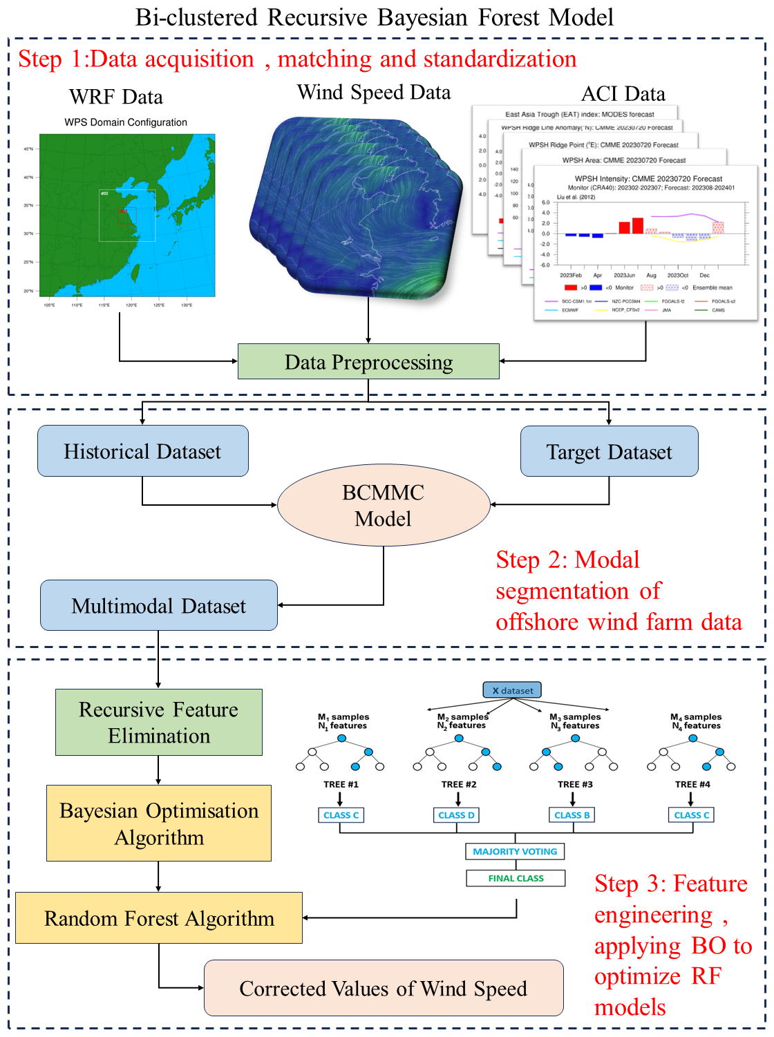
Figure 1 BCRBR model flow diagram to correct for predicted wind speed by WRF.

Table 1 Names of input features and their abbreviations.

The flow chart of the hybrid model used in this study is shown in Fig. 1 and consists of the following three steps.

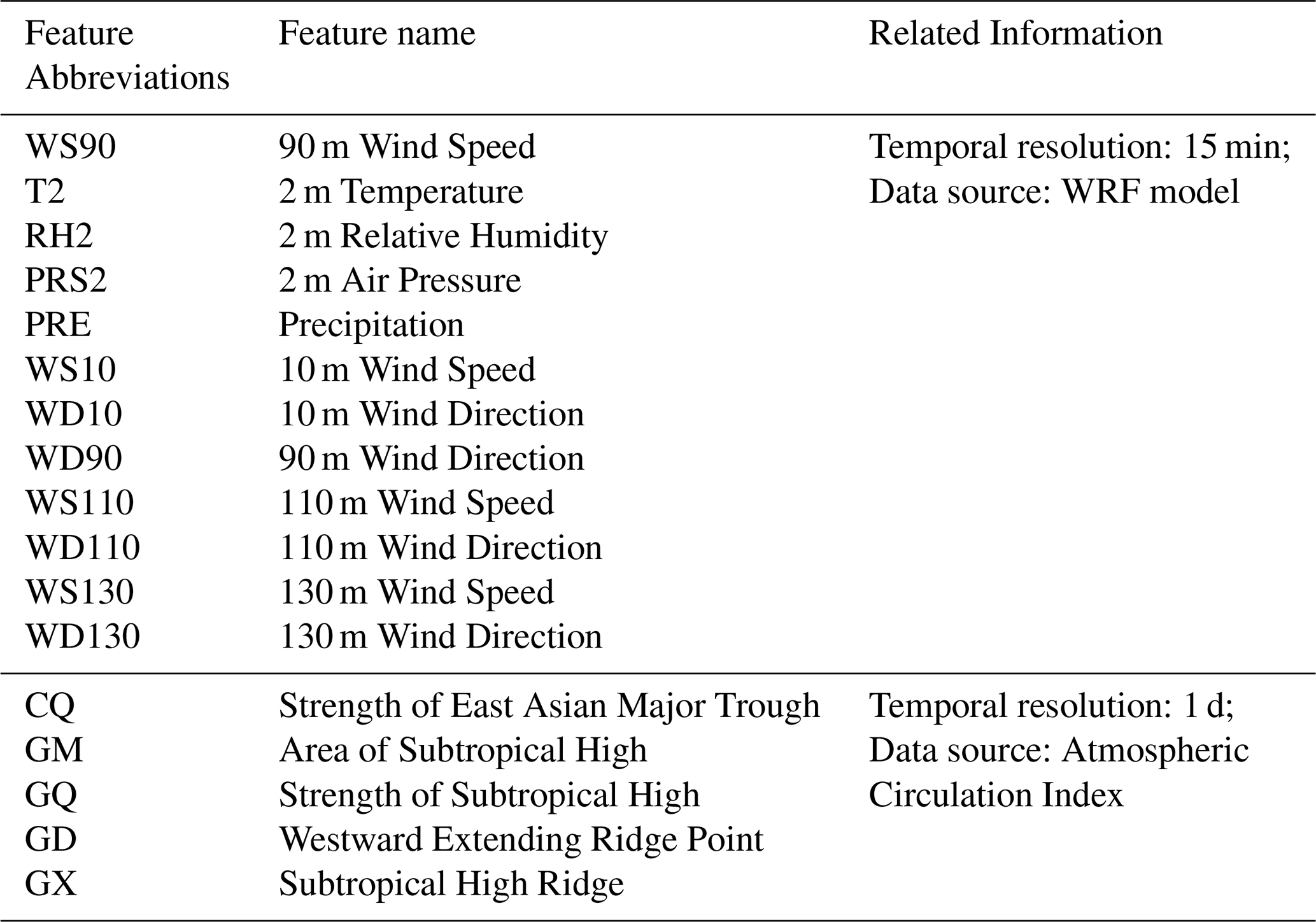
• Step 1 is related to data preprocessing where we used three initial datasets, namely WRF forecast data, observed wind speed data and atmospheric circulation data. Twelve groups of data were selected from the WRF forecast, including 10, 90, 110, and 130 m wind speeds, 2 m temperature, 2 m relative humidity, surface air pressure, and precipitation. The forecast data were interpolated to the latitude and longitude of the target wind farm using a bilinear interpolation method from the WRFOUT grid point weather forecast data. The atmospheric circulation data included five ACIs. All data was fused on the basis of timestamp linkage to construct the input factors for the BCRBR model. Missing values and outliers were removed from the dataset and the data was standardized to ensure a more stable and efficient training process for the model. Table 1 shows the feature names and their abbreviations of the input model.

• Step 2 of Fig. 1 Offshore Wind Farm Data Modal Split. In this study, data from April to July 2023 was used as the historical data used for model training, which is the training set. The data for August 2023 was used as the target dataset used to predict revisions, also known as the test set. A plot of the daily variation of the ACI is given in Fig. 2. The strength of the atmospheric circulation system increased markedly in August and the difficulty of correcting the target dataset increased, especially during the time framed by the black dotted line, when the ACI as a whole fluctuated considerably. We processed the divided historical dataset as well as the target dataset by the BCMMC model to obtain multiple patterns that have been matched between the training set and the test set to form a multi-modal dataset.

• Step 3: Feature engineering and model hyperparameter optimization. For each pattern, the RF algorithm was used first to establish regression models and then RFE was used to screen input features. In this paper, 10 % of the training set was randomly divided as the validation set during model training for hyperparameter optimization, as well as evaluation of the model fit and generalization ability. The trained model was applied to the test set to obtain the corrected wind speed data, and the accuracy of the model was finally evaluated by the wind speed evaluation index.

To comprehensively verify and evaluate the performance, universality and effectiveness of each pattern of the model, the comparison experiment, the robustness experiment, and the ablativity experiment of the model were carried out.

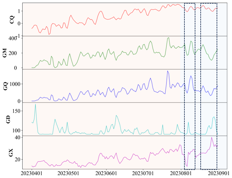
Figure 2 Daily variation of selected ACI during the study period from April 2023 to August 2023.

2.2.2 WRF model

In this study, the WRF 4.2 model developed by the National Center for Environmental Prediction (NCEP) is used, which has the characteristics of portability, extensibility, high efficiency, multiple nesting and rich parametric scheme design (Skamarock et al., 2019). Combined with the three-layer grid nesting configuration, the prediction region is shown in Fig. 3. The number of grids is 150 × 150, 90 × 90 and 150 × 180, and the horizontal grid resolutions were 9, 3, and 1 km, respectively. The center points of the grid were set at 34° N and 120° E. The system is updated every 12 h, once at 00:00 UTC and once at 12:00 UTC, with forecasts for the next 7 d. Considering that the time scale of the meteorological station data in the study area is 15 min, the time interval of the forecast data from the WRF model is also set to 15 min. The meteorological factors selected for the forecast include wind speed in the 10, 90, 110, and 130 m wind directions, temperature of 2 m, relative humidity of 2 m, surface air pressure, and precipitation. Use the bilinear interpolation method to interpolate the WRFOUT grid-based weather forecast data to the latitude and longitude of the target wind farm.

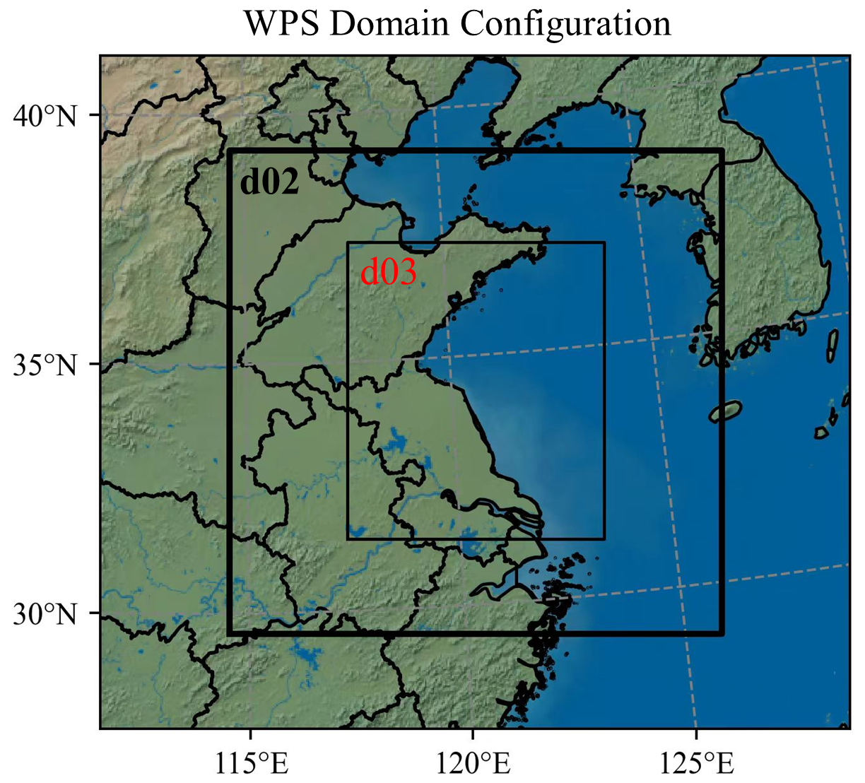
Figure 3 Schematic diagram of the simulation area of the WRF model.

2.2.3 Bi-clustered Meteorological Modal Classification Model

Taking into account the complex meteorological conditions at sea, we proposed using the BCMMC model (Lu, 2025; Sun et al., 2009). A biclustered modal classification of meteorological data was performed from two perspectives: the SLB of mesoscale meteorological systems and weather stability. The first clustering divided the dataset according to the time of day and night to improve the applicability of different periods. Since the synergy of different factors in the large-scale weather system can interfere with the accuracy of wind speed prediction, the second clustering was performed according to the interaction mechanism between different meteorological elements. The structure of the BCMMC model is shown in Fig. 4 in the form of a flowchart.

Figure 4 BCMMC model flow diagram.

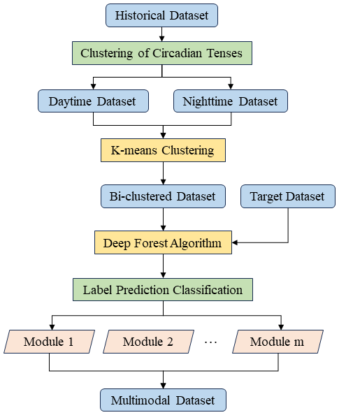
Bi-clustered modal classification

Sea breezes start from late morning to noon, whereas land breezes start at midnight and end at noon (Gille, 2005). According to domestic meteorological standards, 00:00 and 16:00 UTC were used as time points to divide the day and night periods. Temperature and wind speed have a direct impact on weather conditions and can be used as indicators to describe the stability of the weather (Ren et al., 2011).

This study used the K-means clustering method (Lloyd, 1982; MacQueen, 1967) to classify temperature and wind speed as classification features for weather stability. The Euclidean distance is used to measure the similarity between data objects, and the similarity is inversely proportional to the distance (Sinaga and Yang, 2020). By presetting the initial number of clustering centers, clustering can be performed based on the distance of data objects from the centers. During the clustering process, the center positions are continuously updated to minimize the intra-class variance (SSE). The clustering process ends when the SSE is stable or the objective function converges.

Label prediction

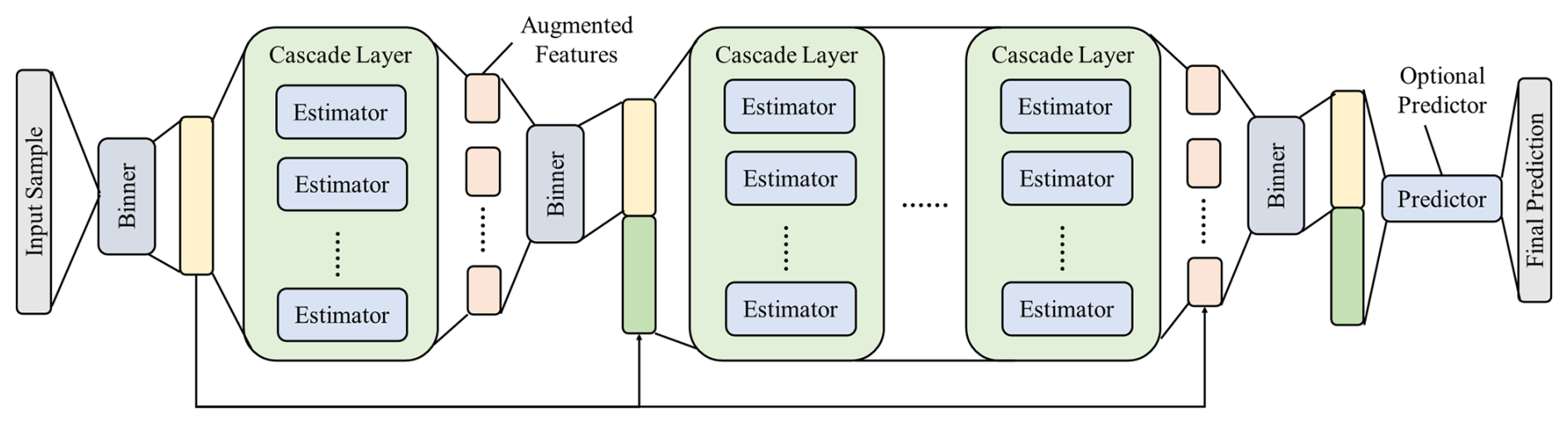
After the historical data set was divided into patterns, the label prediction of the target data set was needed to match the corresponding historical data, and the multi-modal model was formed by combining them. The Deep Forest algorithm (DF) (Zhou and Ji, 2019) is a new tree-based model that can be comparable to the deep neural network proposed by Professor Zhou Zhihua and Dr. Feng Ji on 28 February 2017. Its structure is shown in Fig. 5. DF is a powerful ensemble learning method, also known as gcForest with a multigranularity scan. These are the two core concepts in DF, cascade forest, and multigranularity scans. DF combines the advantages of RF and deep learning, and has advantages in handling high-dimensional data, automatic feature selection, and ensemble learning, making it a powerful classification method with good generalization ability and robustness. In addition, DF is naturally resistant to overfitting (with its cross-validation process). A better result can be obtained without any parameter adjustment.

Figure 5 The structure of DF.

2.2.4 Elimination of recursive characteristics

RFE (Guyon et al., 2002) is a feature selection method used to select the most important features to improve model performance or reduce computational cost. It works by recursively training the model and removing features with minimal impact on performance in each round, continuing this process until a specified number of features or a performance threshold is reached. Therefore, we focus on the features that substantially contribute to the performance of the model and improve the generalizability and efficiency of the model (Lee et al., 2022).

2.2.5 Parameter optimization

Bayesian Optimization

The BO algorithm (Mockus, 1975) is commonly used to optimize machine learning models or other tasks that require parameter tuning (Shahriari et al., 2016). BO uses Bayesian statistical inference to construct a probabilistic model of the parameter space and updates the model based on historical observations at each iteration. This allows for smarter selection of the next combination of parameters to evaluate to maximize the outcome of the objective function. Here are the steps to implement the BO method:

• Step 1: Define the objective function. First, define the objective function f(x) to be optimized, where x is a set of hyperparameters.

• Step 2: Initialize the Gaussian process: Construct a Gaussian process $GP\left(m\left(x\right),k\left(x,x^{\prime }\right)\right)$, where m(x) is the mean function and $k\left(x,x^{\prime }\right)$ is the kernel function. Usually, set m(x)=0 and choose an appropriate kernel function, such as the Gaussian kernel:

  $$\begin{array}{}\text{(1)}& k\left(x,x^{\prime }\right)=\exp \left(-{\displaystyle \frac{{∥x-x^{\prime }∥}^{\mathrm{2}}}{\mathrm{2}{\mathit{\sigma }}^{\mathrm{2}}}}\right)\end{array}$$

• Step 3: Initial sampling. Select an initial set of hyperparameters x₁, x₂, …, x_n, compute the corresponding objective function values y₁, y₂, …, y_n, and use this data to construct the initial Gaussian process model.

• Step 4: Update the Gaussian process model: Based on the current Gaussian process model, calculate the next hyperparameter x_n+1 to sample, such that the expected improvement (EI) is maximized:

  $$\begin{array}{}\text{(2)}& \begin{array}{rl}{x}_{n+\mathrm{1}}& ={\mathrm{argmax}}_x\mathrm{EI}\left(x\right)\\ & =\mathbb{E}\left[max\left(f\left(x\right)-f\left(x^{+}\right),\mathrm{0}\right)\right]\end{array}\end{array}$$

  where x⁺ is the current best known hyperparameter.

• Step 5: Iterative optimization. For the newly sampled hyperparameter x_n+1, compute the objective function value y_n+1 and update the Gaussian process model. Repeat step 4 until the specified number of iterations or convergence criteria are met.

• Step 6: Output the optimal hyperparameters. Throughout the optimization process, record all the hyperparameters sampled and their corresponding objective function values. Finally, output the set of hyperparameters that corresponds to the minimum objective function value as the optimal hyperparameters.

10-fold cross-validation method

At each step of using the BO algorithm, 10-fold cross-validation is used to evaluate the performance of the current hyperparameter configuration to avoid BO falling into a locally optimal solution. 10-fold cross-validation (Breiman et al., 1984) is a commonly used evaluation method for machine learning models to evaluate their generalizability on unseen data (Stone, 1974). In each iteration, the dataset is randomly divided into 10 equal-sized subsets (folds). One of the folds is selected as the validation set and the remaining 9 folds are used as the training set to train the model and evaluate the performance on the validation set. This process is repeated 10 times, each time using a different validation fold. The performance metrics of the 10 times are averaged as the final evaluation result of the model.

2.2.6 Random forest algorithm

The RF algorithm (Breiman, 2001) combines multiple decision trees to perform prediction and classification tasks. The RF modeling process is as follows.

First, define the wind speed prediction training set X_i→Y_i, where Y_i is the real value in the RF prediction model, mapped to the real value of wind speed of the ith sample in the data; X_i is the feature vector established by the meteorological elements of the ith sample in the data, and is denoted by $\mathit{\{}{I}_{i\mathrm{1}},I_{i\mathrm{2}},\mathrm{\dots },I_{in}\mathit{\}}\to X_i$ denote the n influence factors of the ith sample.

Next, based on determining the training set, a single regression decision tree is built. Through the feature vector X and its corresponding true value Y in the training sample, the split variable and split value are searched, and the regression decision tree divides the whole vector space into m partitions $\mathit{\{}{R}_{\mathrm{1}},R_{\mathrm{2}},\mathrm{\dots },R_n\mathit{\}}$. For any partition of which can be mapped to the model C_m, the vector space is divided into two parts by the value of a feature, and the expression is

$$\begin{array}{}\text{(3)}& {\displaystyle }{R}_{\mathrm{1}}\left(j,s\right)=\left\{I|I_j\le s\right\}\text{(4)}& {\displaystyle }{R}_{\mathrm{2}}\left(j,s\right)=\left\{I|I_j\le s\right\}\end{array}$$

where, j represents an influencing factor and s represents the value when splitting. The objective function for performing the vector space split variable and split value search is

$$\begin{array}{}\text{(5)}& z:\underset{j\cdot s}{min}\left[\underset{c_{\mathrm{1}}}{min}\sum _{x_i\mathit{ϵ}{R}_i\left(j\cdot s\right)}{\left(y_i-c_i\right)}^{\mathrm{2}}+\underset{c_{\mathrm{2}}}{min}\sum _{x_i\mathit{ϵ}{R}_{\mathrm{2}}\left(j\cdot s\right)}{\left(y_i-c_{\mathrm{2}}\right)}^{\mathrm{2}}\right]\end{array}$$

where, z is the minimum variance of the real value of wind speed; y_i is the real wind speed value of the ith sample; x_i is the corresponding value of the ith sample's impact factor vector; c₁ is the real mean value of wind speed in the first part; c₂ is the mean real value of wind speed in the second part.

Finally, build the entire RF based on a single decision tree. The RF prediction value is the average of the predicted values of all decision trees.

2.2.7 Evaluation metrics

In this study, the effect of the model was evaluated by statistical test. We use the following statistics: Root Mean Square Errors (RMSE), relative mean absolute error (rRMSE), and mean absolute error (MAE), where smaller values indicate smaller errors. The mean absolute percentage error (MAPE) has a value range of [0, +∞], the smaller the value, the better the prediction model has, a MAPE of 0 indicates a perfect model, and a MAPE greater than 100  % indicates a poor model. R, also known as the correlation coefficient, was used to verify the degree of “linear” relationship predicted by the model. The formulas for the four statistics are given below:

$$\begin{array}{}\text{(6)}& {\displaystyle }\mathrm{RMSE}=\sqrt{{\displaystyle \frac{\mathrm{1}}{n}}\sum _{i-\mathrm{1}}^n{\left({\widehat{y}}_i-y_i\right)}^{\mathrm{2}}}\text{(7)}& {\displaystyle }\mathrm{rRMSE}={\displaystyle \frac{\sqrt{\frac{\mathrm{1}}{n}{\sum }_{i=\mathrm{1}}^n{\left(y_i-{\widehat{y}}_i\right)}^{\mathrm{2}}}}{\frac{i}{n}{\sum }_{i=\mathrm{1}}^n{y}_i}}\times \mathrm{100}\mathit{\%}\text{(8)}& {\displaystyle }\mathrm{MAE}={\displaystyle \frac{\sum _{i=\mathrm{1}}^n\left|y_{i-}{\widehat{y}}_i\right|}{n}}\text{(9)}& {\displaystyle }\mathrm{MAPE}=\left({\displaystyle \frac{\mathrm{100}}{n}}\right)\sum _{i=\mathrm{1}}^n\left|{\displaystyle \frac{y_i-{\widehat{y}}_i}{y_i}}\right|\text{(10)}& {\displaystyle }R={\displaystyle \frac{\sum _{i=\mathrm{1}}^n\left(x_i-\stackrel{\mathrm{‾}}{x}\right)\left(y_i-\stackrel{\mathrm{‾}}{y}\right)}{\sqrt{{\sum }_{i=\mathrm{1}}^n{\left(x_i-\stackrel{\mathrm{‾}}{x}\right)}^{\mathrm{2}}}\sqrt{{\sum }_{i=\mathrm{1}}^n{\left(y_i-\stackrel{\mathrm{‾}}{y}\right)}^{\mathrm{2}}}}}\end{array}$$

where ${\widehat{y}}_i$ is the ith predicted value, y_i is the ith observation, n is the total number of time samples, and $\stackrel{\mathrm{‾}}{y}$ is the average of the observations. Forecast accuracy (FA) refers to the percentage of absolute deviations in wind speed forecasts that are not greater than 1 m s⁻¹. The formula is as follows:

$$\begin{array}{}\text{(11)}& \mathrm{FA}={\displaystyle \frac{N_{\mathrm{r}}}{N_{\mathrm{f}}}}\times \mathrm{100}\mathit{\%}\end{array}$$

where N_r is the number of samples where the absolute deviation of the wind speed forecast is not more than 1 m s⁻¹, and N_f is the number of samples forecasted.

3 Results and discussion

3.1 Results of the BCMMC model

The preprocessed training and test sets were loaded into the BCMMC model for modal classification. After the day and night division, the training set was divided into 4 clusters for each of the daytime and nighttime hours using K-means clustering. A total of 8 groups were waiting to be matched with the test set. Table 2 indicated that the data distribution within each group was concentrated over 2–3 months with a uniform time distribution. There was no concentration in any particular month, demonstrating a good clustering effect.

Table 2 Distribution of bi-clustered data. The bold clusters are clusters that were matched to the test set to form multimodal data.

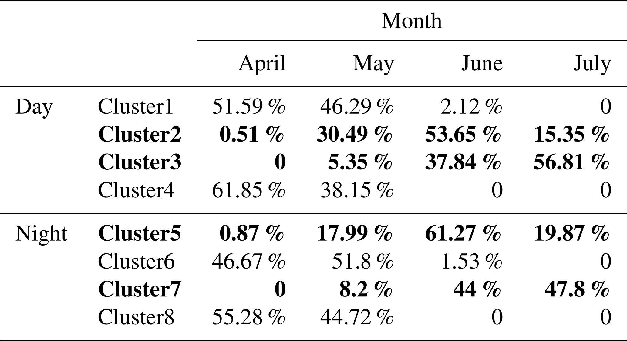
Each cluster represented the meteorological characteristics of different periods, which was conducive to subsequent analysis and modeling.

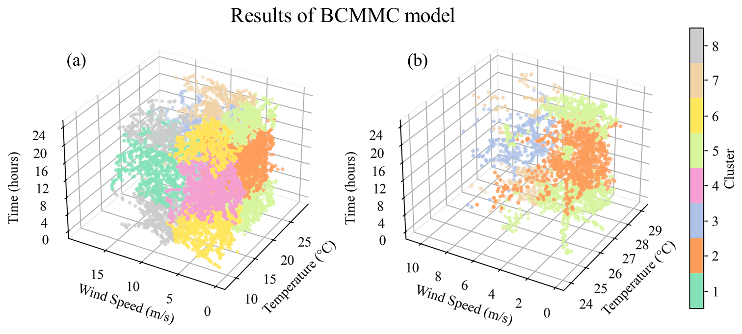
Figure 6 Results of the BCMMC model. (a) Bi-clustering classification, and (b) label prediction.

The daytime and nighttime periods of the test set were processed by the DF algorithm, and two clusters were predicted for each, as shown in Fig. 6. These four clusters corresponded to the two scenarios of low and high wind speeds under hot weather conditions, reflecting the stability of the weather or not. The clusters of the test set were matched with the clusters of the corresponding training set to form multi-modal data. The BCMMC model was divided into four modes, and modes 1, 2, 3, and 4 corresponded to the four meteorological features of daytime smooth, daytime smooth, nighttime smooth, and nighttime smooth in August 2023, respectively.

3.2 Results of RFE and Parameter Optimization

The RF regression models were established for the four patterns and the parameters were optimized. The correlation analysis (Fig. 7) showed that the actual wind speeds of the patterns were strongly correlated with the wind speeds at different levels, meteorological factors, and some ACIs, indicating that the other factors and the large-scale circulation system have an important influence on wind speed prediction. The importance ranking of the features (Fig. 8) showed that the wind speed at different levels was the main characteristic, while the contributions of ACI and other meteorological factors varied according to the patterns, and the fluctuation of the RMSE with the number of features (Fig. 9) in the RFE screening of the input features of the modal models was due to the correlation between the features and the small amount of data.

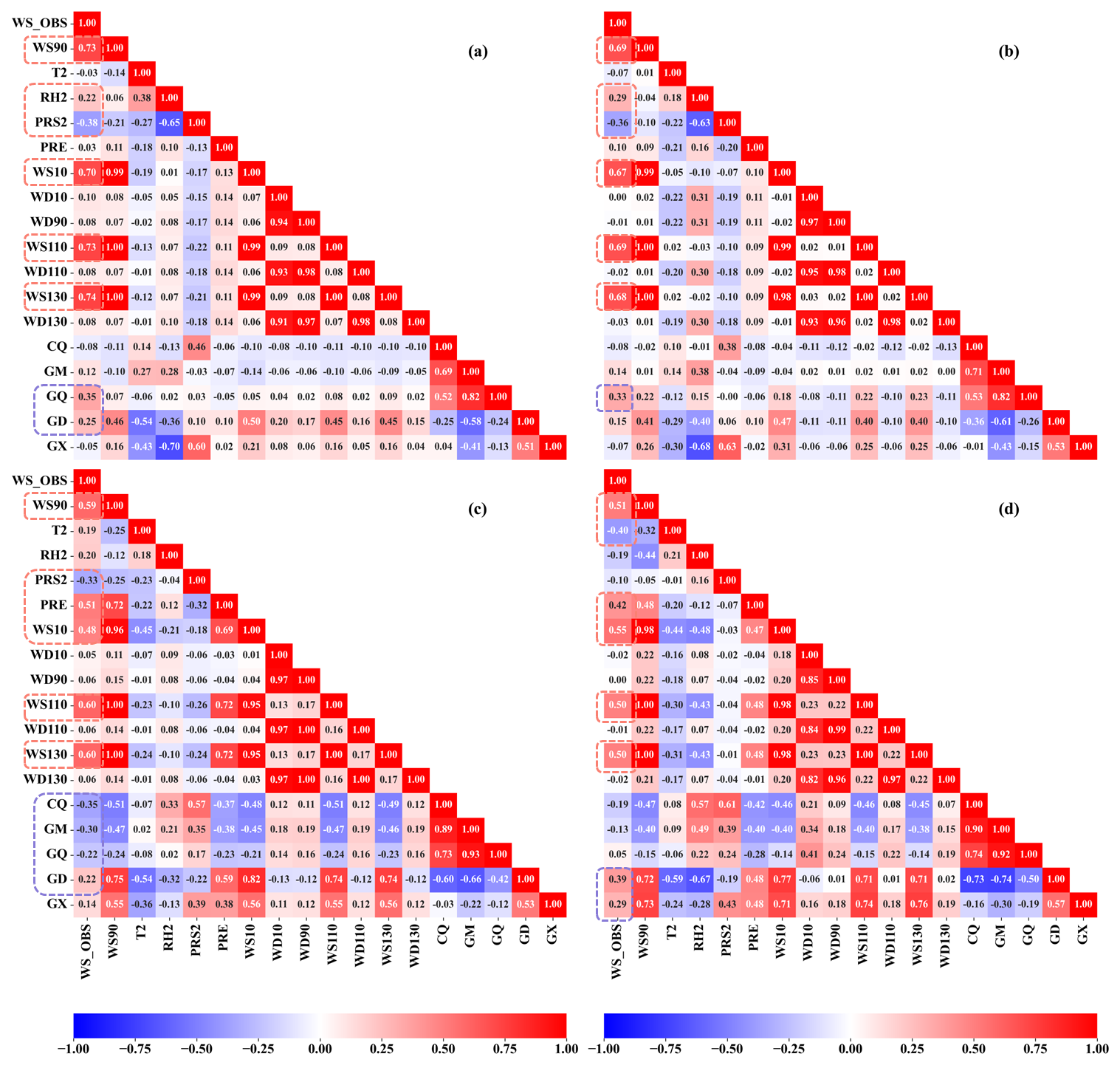
Figure 7 Correlation between variables of the 4 patterns. Panels (a)–(d) represent patterns 1, 2, 3, and 4 respectively. The red dashed boxes represent highly relevant meteorological elements; blue dashed boxes represent highly relevant ACI.

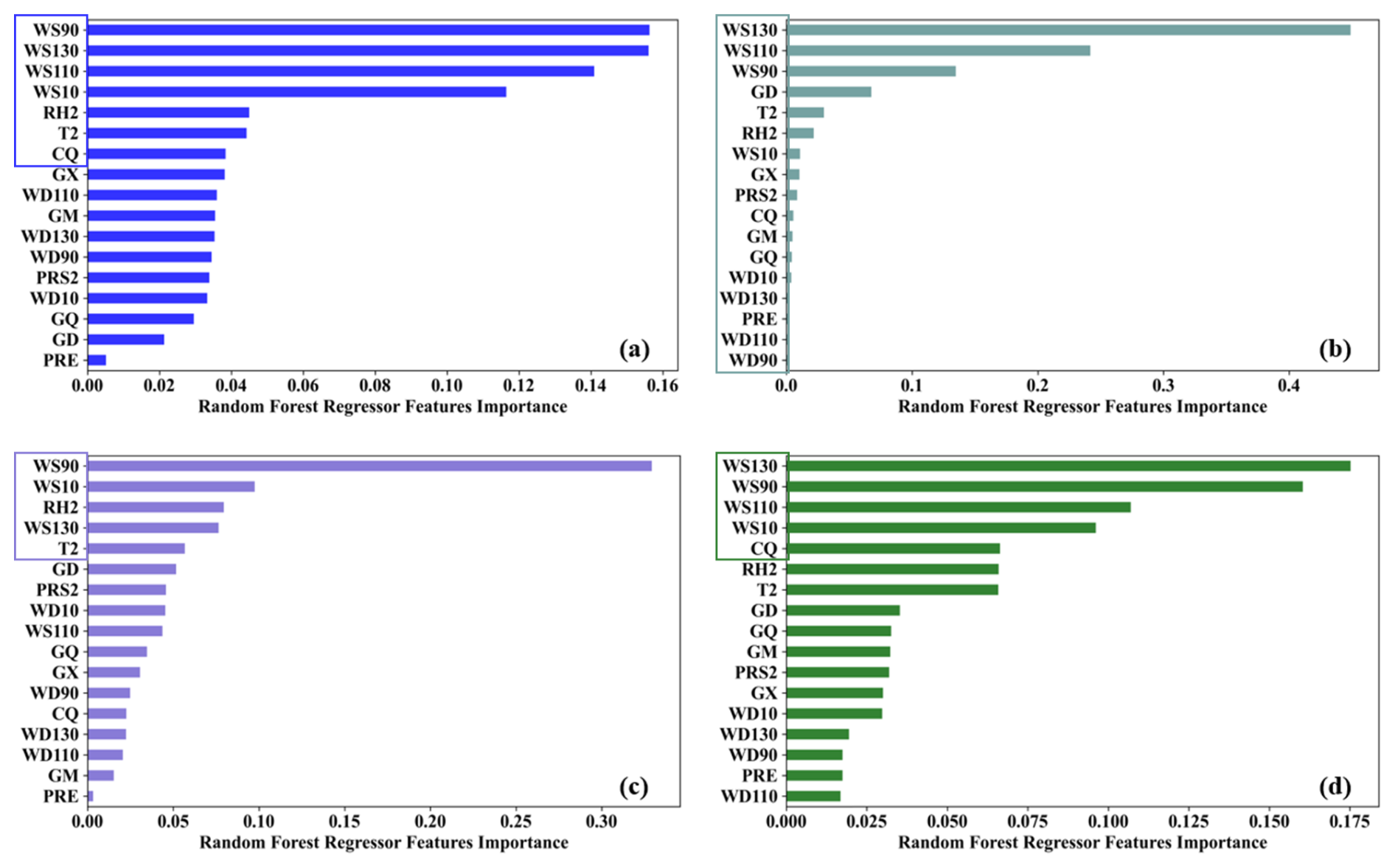
Figure 8 Importance of the 4 patterns. Panels (a)–(d) represent patterns 1, 2, 3, and 4 respectively. The framed features represent the final input.

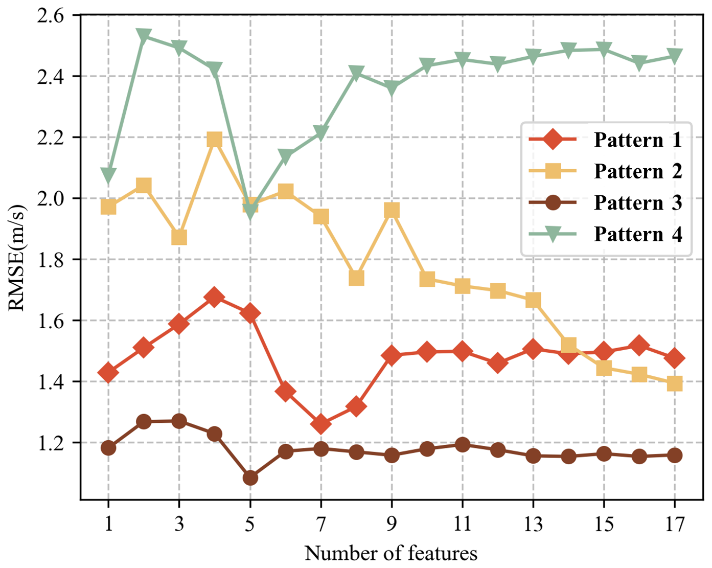
Figure 9 The result of RFE, variation of each pattern error (RMSE) with the number of features.

The number of features with the lowest error was chosen as the final input features of the models: pattern 1 had 7 final inputs of 90, 130, 110, 10 m wind speed, 2 m relative humidity, and 2 m temperature with CQ; pattern 2 had all 17 features selected as final inputs; pattern 3 had 5 features of 90, 10 m wind speed, and 2 m relative humidity, and 130 m wind speed, and 2 m temperature; and pattern 4 had 5 features of 130, 90, 110, 10 m wind speed, and CQ. After feature selection, the best parameters of the models confirmed by the BO algorithm are shown in Table 3.

Table 3 The best hyperparameters of the models.

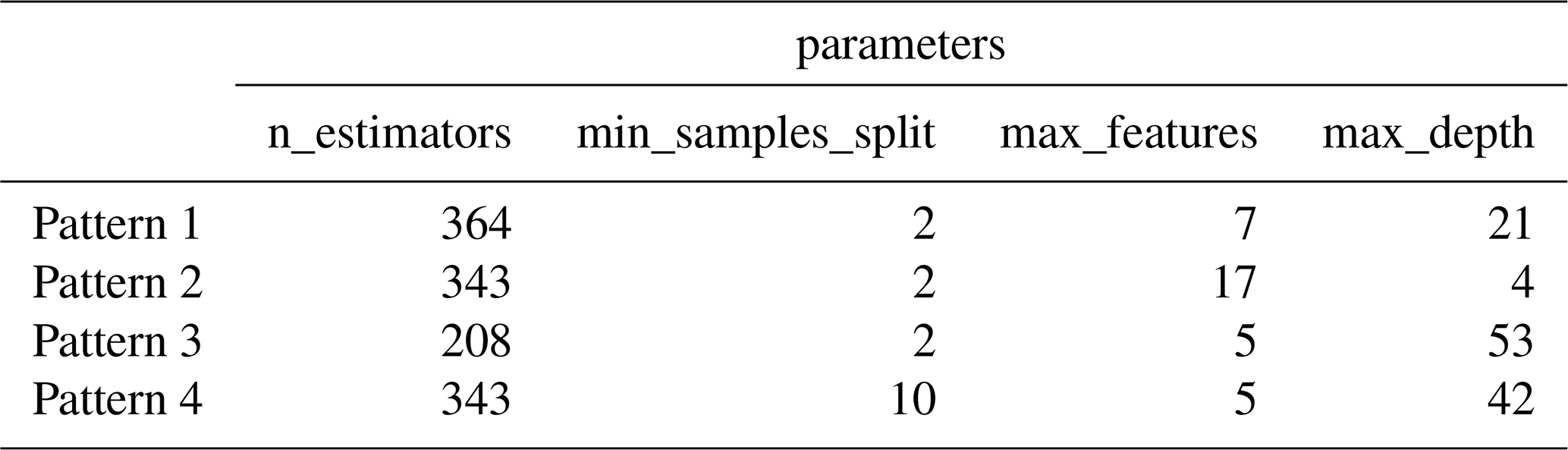
The ACI reflected the complex relationship between meteorological variables and could improve the prediction performance of the model by correlated with other characteristics. The input features of all patterns except pattern 3 included the ACI, which indicated that atmospheric circulation played an important role in the correction of the wind speed prediction and had a significant effect on the model prediction. Pattern 2 was a non-smooth period during the daytime, which was affected by daylight, topography, and other factors, with frequent and complex changes of large-scale weather systems, and required highly correlated multi-featured factors as inputs to characterize the complex relationship with the fast-changing wind speeds. Pattern 3 was a stable period at night, with weak activity of large-scale weather systems and relatively static pressure, and no ACI was needed as a reference. Patterns 1 and 4 only screened CQ, a weather system that is an important indicator of changes in the offshore wind farm.

3.3 Results of wind speed correction

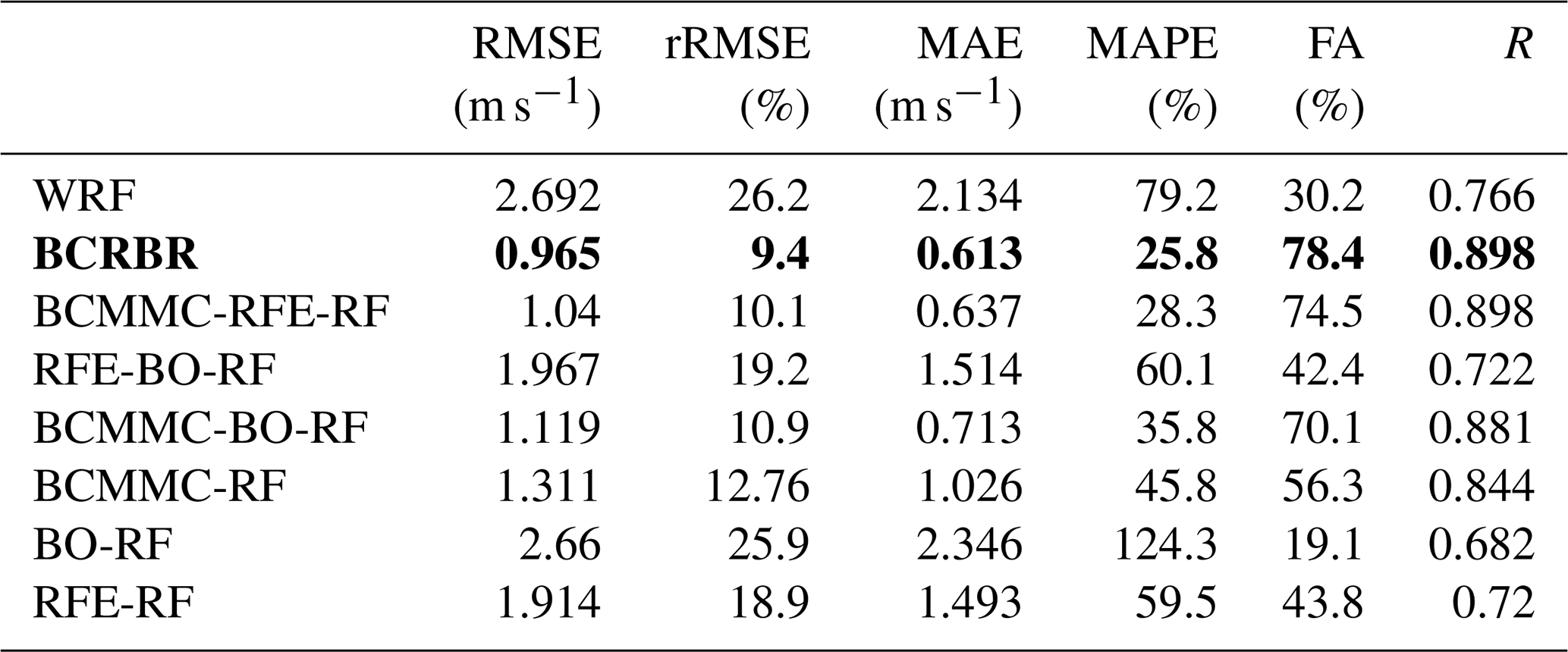
The corrected results for the four patterns were exported and aggregated to obtain the corrected results for the final August 2023 test set. The statistical errors are shown in Table 4, and the wind speed errors of each pattern after the correction of the BCRBR model were reduced to different degrees compared to the WRF forecast, the daytime dataset represented by patterns 1 and 2 showing better prediction performance compared to the nighttime dataset represented by patterns 3 and 4. On the contrary, the RMSE of the wind speed in the test set decreased from 2.692 to 0.965 m s⁻¹, an overall reduction of 64.15 %, and the correlation coefficient, R, increased from 0.766 to 0.898. A comparison of the regression scatter density plots for each dataset (Fig. 10) showed that the wind speed forecasts of the WRF system were overall large. Patterns 1 and 3 correspond to a small range of wind speed values; in contrast to Patterns 2 and 4, which correspond to a large range of wind speed values, there were more outliers in the dataset, which would have a certain impact on the model's generalization performance and lead to a decrease in the prediction performance.

Table 4 The four patterns and aggregated results. Values in bold are used to highlight the models/datasets that performed best in the experiment.

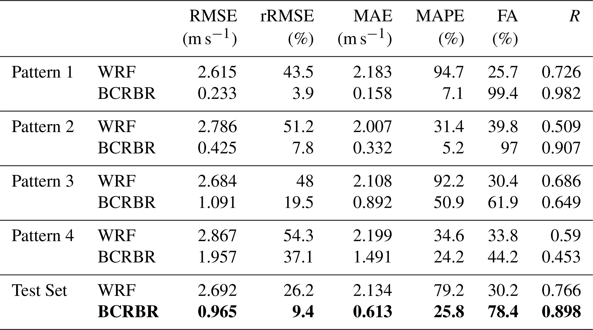
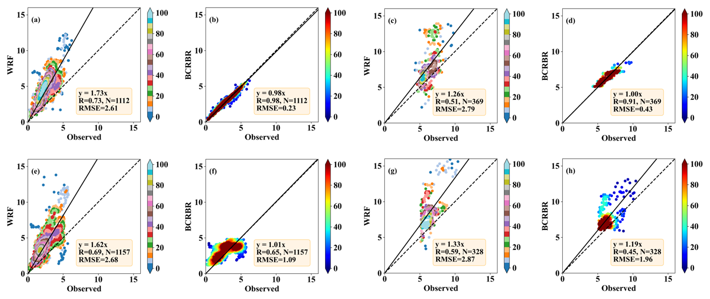
Figure 10 Regression scatter density plots for WRF forecast and the forecast of the BCRBR model. Panels (a), (c), (e), (g) represent patterns 1, 2, 3, 4 respectively for WRF, and panels (b), (d), (f), (h) represent patterns 1, 2, 3, 4 respectively for BCRBR.

Figure 11 Box plot of daily changes in forecast and observed values for August 2023.

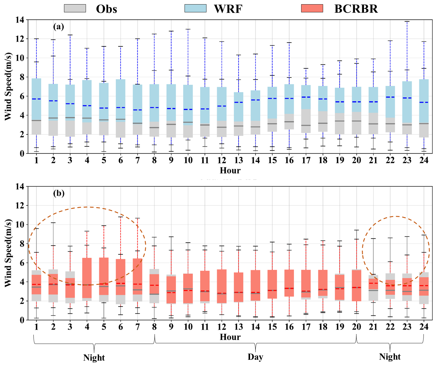
The daily variation of wind speed in the test set was further analyzed, and the boxplot of the daily variation of actual wind speed between the WRF forecast and the BCRBR model forecast was shown in Fig. 11. The distribution of the actual data (grey) was relatively concentrated, with a median between 3 and 4 m s⁻¹ and fewer outliers. The distribution of the WRF forecast data (blue) was more discrete, the median was more different from the observed data in different periods, and there were more outliers and obvious overestimation, which indicated that the WRF model had greater uncertainty in simulating the wind speeds. The median of the BCRBR model forecast data (in blue) was in better agreement with the actual observations for most of the periods, but there were some periods of slightly higher or lower values. In addition, as seen in the dashed box portion of Fig. 11b, the wind speed trend was smooth during the daytime hours, while the wind speed during the nighttime hours was larger and subject to larger fluctuations, which made it more difficult to predict, and that is why the wind speed prediction for the two patterns during the daytime hours was more accurate than the two patterns during the nighttime hours.

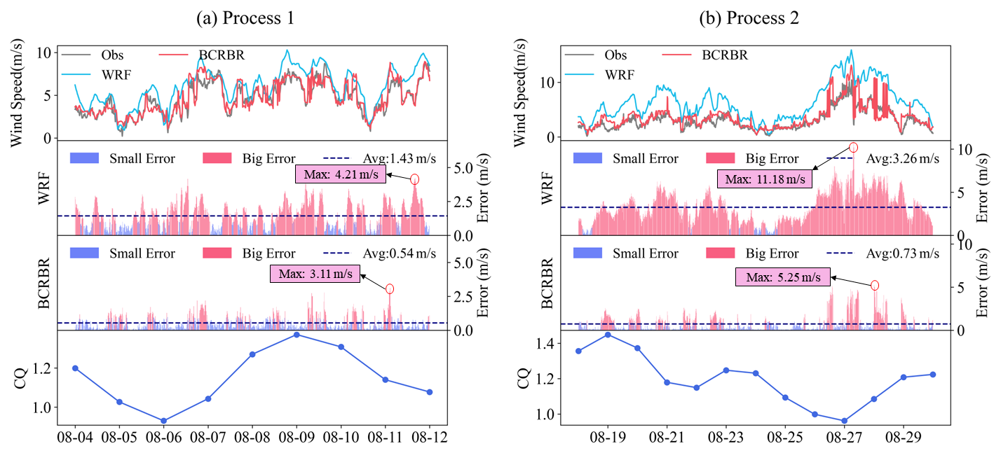
Figure 12 Time series plots of wind speed values, errors, and CQ during abrupt atmospheric circulation changes. (a) Process 1, (b) Process 2.

From the above, it can be seen that wind speed was more difficult to predict in the unstable state of the atmosphere, and the change in atmospheric circulation was closely related to wind speed. Since CQ made a larger contribution compared to other ACIs in the BCRBR model for most patterns, here CQ was used as an indication of the change in weather stability, focusing on the comparison of the wind speed forecasts during the two abrupt ACI changes in the black box in Fig. 4. Since FA was defined as the percentage of wind speed forecasts with absolute deviation not greater than 1 m s⁻¹, here the absolute deviation less than or equal to 1 was defined as a small error; otherwise, it was a large error. Comparing the time series plots of wind speed values and errors in the two processes (Fig. 12), it is easy to find that the WRF system produced a large and concentrated bias in the forecast when the weather was not stable and the wind speed error was significantly reduced after the revision of the BCRBR model. The maximum error of the two processes decreased from 4.21 to 3.11 and 11.18 to 5.25 m s⁻¹, and the average error decreased from 1.43 to 0.54 and 3.26 to 0.73 m s⁻¹, respectively. In particular, the corrected effect of process 2 was a good example of the validity of the BCRBR model.

Table 5 The optimal hyper-parameters found for each model.

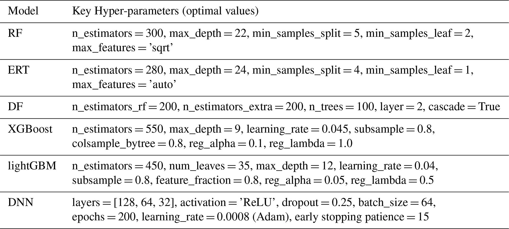
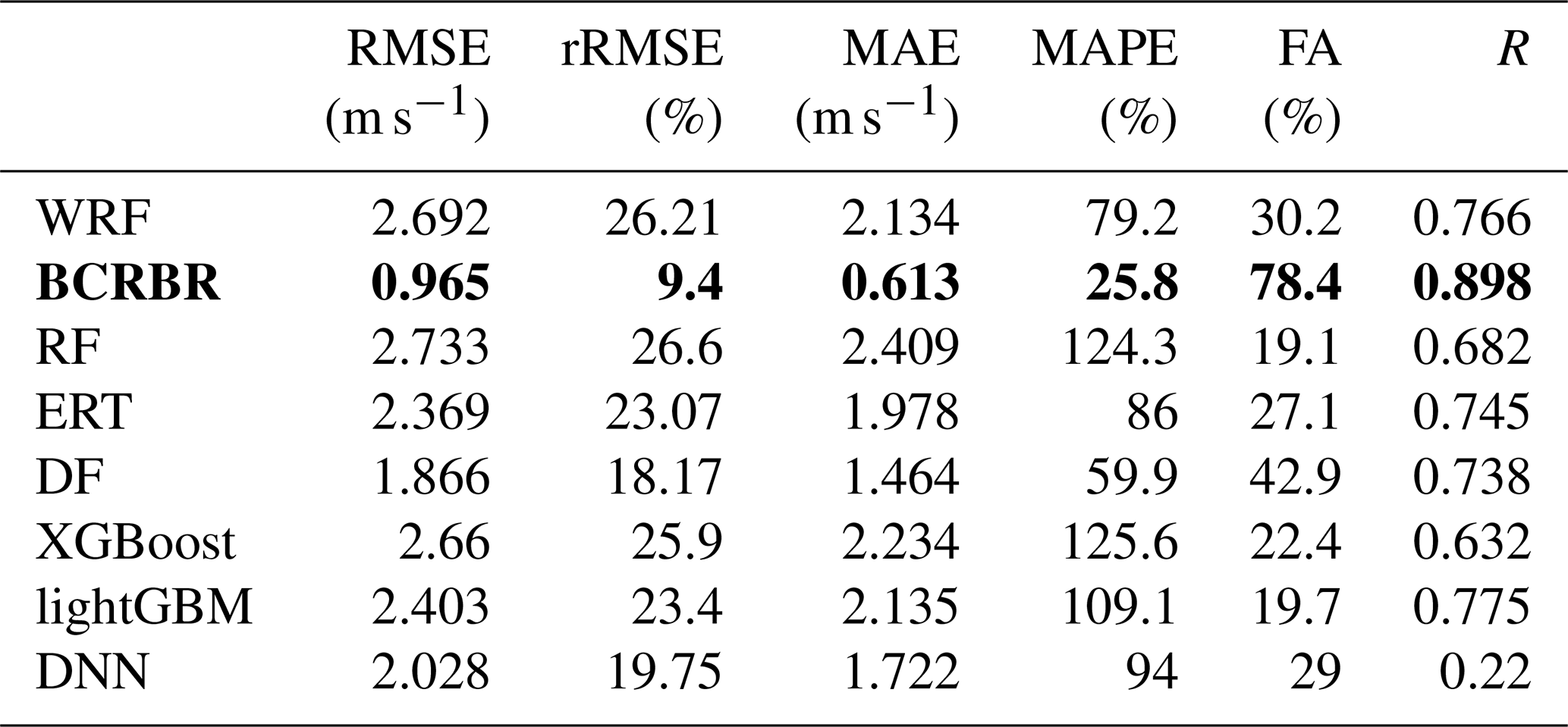
Table 6 Comparing the performance of the models in the experiment in terms of error metrics. Values in bold are used to highlight the models/datasets that performed best in the experiment.

3.4 Comparison experiment

To comprehensively evaluate the wind speed prediction performance of the BCRBR model, we selected popular machine learning and deep learning methods in the wind power field, such as the RF, ERT, DF, XGBoost, lightGBM, and DNN models, and used the same dataset to predict wind speed for comparison experiments. The optimal hyper-parameters found for each model are summarized in Table 5. Table 6 shows the error metrics of the prediction effects of each model. After comparison, the BCRBR model performed the best in all error metrics and demonstrated good performance in the limited dataset, highlighting its strong competitiveness. The Taylor diagram in Fig. 15a visually displays the correction effects of each model, with the BCRBR model being closest to the reference point, indicating that its prediction results were closest to the measured values, had the smallest error, and exhibited the best prediction performance.

3.5 Ablativity experiment

To verify the validity of each pattern of the BCRBR model, an ablativity experiment was performed on the model. After removing each or some of the patterns in the model, respectively, the results after prediction on the same dataset were shown in the Taylor diagram in Fig. 13b, and the model that was closest to the observed value was still the BCRBR model.

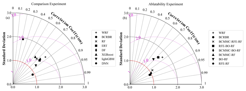
Figure 13 Taylor diagrams of the predictions of August 2023 for each model. (a) Comparison experiment, (b) ablativity experiment.

Statistically, it is not difficult to find that BCRBR performed the best in all the error indicators (Table 7). Interestingly, as long as the models containing the BCMMC pattern can get good prediction results, the performance was better than other models, indicating that the BCMMC model played a key role in improving the accuracy of wind speed prediction.

Table 7 Performance of each model in ablativity experiment. Values in bold are used to highlight the models/datasets that performed best in the experiment.

3.6 Robustness experiment

The BCRBR model was applied to a mountainous wind farm in Jiangxi Province and a robustness experiment was conducted with data from 1 December 2023 to 19 March 2024 to test its generality. The data from December 2023 to February 2024 and March 2024 were used for training and testing, respectively. The time series of WRF predicted values, BCRBR predicted values, observed values, and forecast errors are given in Fig. 14, and the BCRBR model had a better correction effect, with the average error reduced from 1.84 to 1.23 m s⁻¹, and the maximum error decreased from 7.04 to 5.35 m s⁻¹, compared with the prediction of WRF. The blue dotted box in Fig. 14 exhibited the most effective correction, whereas the red dotted box showed a less effective correction, with a focus on high-wind-speed values. There was still potential for further improvement in the model.

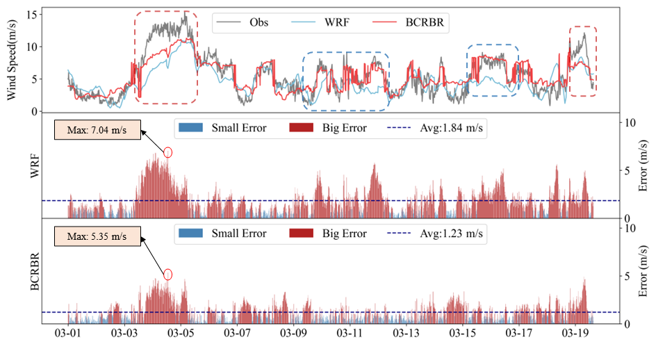
Figure 14 Time series plot of wind speed values and errors for WRF forecast and the BCRBR model forecast.

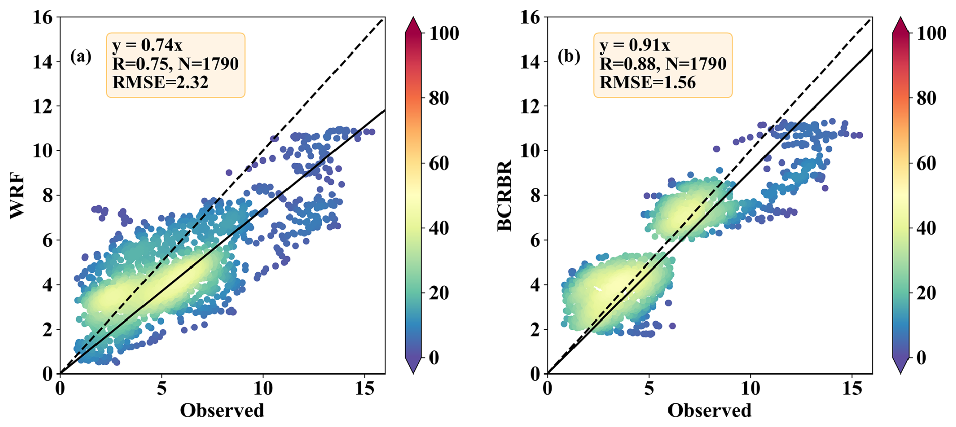
The regression scatter density plot of wind speed is shown in Fig. 15, comparing with the WRF forecast, the RMSE of wind speed decreased from 2.32 to 1.56 m s⁻¹, and the correlation increased from 0.75 to 0.88. The linear distribution of the scatter had a more pronounced trend, and the regression line was closer to the congruent line y=x. In summary, the BCRBR model also had a good wind speed correction ability in different regions of the wind farm and a strong generality.

Figure 15 Regression scatter plot of wind speed. (a) WRF forecast, (b) BCRBR model forecast.

In the robustness experiment, the overall accuracy of wind speed prediction for the wind farm in Jiangxi Province of China was slightly lower as compared to the offshore wind farm in Jiangsu Province, mainly because the wind farm in Jiangxi Province is a mountainous wind farm with a more complex topography than an offshore wind farm. In intricate terrain, numerous factors affect wind speed, including the drag effect caused by the ruggedness of mountain surfaces on the atmosphere, as well as localized circulations like valley winds and slope winds, stemming from the uneven heating and cooling of mountainous regions.

In the future, the following methods will be considered to enhance the accuracy of wind speed prediction in mountain areas. Incorporating terrain factors and underlying surface parameters, such as terrain height, slope, roughness, etc., as input features in the wind speed prediction model. Increasing the density and quality of observations, particularly in complex topographic regions, to provide a larger sample size for model training and validation.

4 Conclusions

This study presented a multimodal short- and medium-term wind speed prediction correction approach based on bi-clustering and machine learning, aiming to address the crucial scientific problems of incomplete consideration of influencing factors and limited feature extraction in traditional wind speed prediction. In this paper, the BCRBR model was innovatively constructed, with offshore wind farms as the research object, and the complex influence mechanisms of sea-land breeze and atmospheric circulation on wind speed were thoroughly considered from a meteorological perspective. By introducing bi-clustering strategies and innovative features such as atmospheric circulation indices, precise correction of wind speed predictions was achieved in this study. Compared to the traditional WRF model, the errors of the corrected wind speed predictions were significantly reduced, specifically the following. RMSE, rRMSE, MAE and MAPE all decreased by more than 60 %, the wind speed forecast accuracy rate increased from 30.2 % to 78.4 %, and the correlation coefficient R increased from 0.77 to 0.9.

This research not only offers new thoughts for wind speed prediction in methodology, but also provides data source guarantees to enhance the accuracy of wind power prediction. The research findings have significant theoretical value and practical significance in promoting the large-scale development of wind power and the sustainable development of power systems. The results of comparative experiments demonstrated that the BCRBR model outperforms the prevalent single-model prediction methods in the current literature. The results of the robustness experiments indicated that this method also performed better than the traditional WRF model in the prediction of wind speed in mountain wind farms in terms of various performance indicators, but there was a slight disparity compared to the results in offshore wind farms, which provided an important direction for subsequent improvement.

Future research will focus on the following directions to improve the accuracy of wind speed prediction in mountainous areas:

1. Integrating terrain factors and surface parameters – such as elevation, slope, and roughness – as input features for wind speed prediction models.

2. Enhancing the quality of observational data, especially in complex terrain regions, by implementing data quality control protocols to supply more reliable samples for model training and validation.

3. Refining model parameters and extracting informative features to improve prediction performance under complex terrain conditions, thereby broadening the applicability of the method and supporting efforts to mitigate instability in renewable energy generation.

Appendix A: List of abbreviations

Abbreviations	Full name
NWP	Numerical Weather Prediction
WRF	Weather Research and Forecasting
SLB	Sea-land Breeze
SSE	The Sum of Squares due to Error
DF	Deep Forest
BO	Bayesian Optimization
RFE	Recursive Feature Elimination
RF	Random Forest
RMSE	Root Mean Square Errors
rRMSE	Relative Root Mean Square Errors
MAE	Mean Absolute Error
MAPE	Mean Absolute Percentage Error
FA	Forecast Accuracy
R	Correlation Coefficient
ACI	Atmospheric Circulation Index
ERT	Extremely Randomized Trees
DNN	Deep Neural Networks
BCMMC	Bi-clustered Meteorological Modal Classification
RBR	Recursive Bayesian Forests
BCRBR	Bi-clustered Recursive Bayesian Forest
HIRLAM	High-resolution Limited Area Model
MM5	Mesoscale Model 5
ECMWF	European Centre for Medium-Range Weather Forecasts