The “Golden Points” and nonequilibrium correction of high-accuracy frost point hygrometers

We introduce a new retrieval protocol for chilled mirror hygrometer measurements that enables balloon-borne frost point measurements in the upper troposphere/lower stratosphere of unprecedented accuracy under conditions of rapidly changing humidity. Chilled mirror hygrometers measure the frost point (or dew point) by quantifying the saturation ratio of the air with respect to the condensed phases of water (ice or liquid). To this end, they attempt to determine the thermodynamic equilibrium of the mirror condensate with the vapor phase by measuring the mirror reflectance, which changes with the amount of condensed material. In the rapidly changing environment along the balloon trajectory, however, the adjustment of the mirror temperature to the new equilibrium point may lead to frequent, damped overshoots or nonequilibrium errors. For the Cryogenic Frost Point Hygrometer (CFH), a balloon-borne chilled mirror instrument of reference quality, we (i) identify points in time along the sounding profile when the mirror is in equilibrium with the gas phase, which we term “Golden Points”, and (ii) correct the measurements under nonequilibrium conditions between these Golden Points. For (i), we identify the points where the suitably smoothed mirror reflectance assumes an extreme value, i.e. a maximum or a minimum. At these extreme points, the CFH mirror temperature represents the frost point with an accuracy better than 0.2 K (resulting from the uncertainties of the mirror temperature sensor and of the precise timing of the Golden Points along the sounding profile). These accurately determined frost points can be used to detect and correct offsets, biases and time lag errors in other humidity sensors flown together with CFH on the same balloon payload, such as the FLASH-B fluorescence hygrometer or the thin-film capacitive hygrometer of the Vaisala RS41 radiosonde. From the surface to approximately 28 km, a frost point uncertainty of 0.2 K corresponds to less than 4 % uncertainty in H₂O mixing ratio (including the uncertainty of 0.3 hPa in the GPS-based pressure measurement of the RS41 radiosonde), provided there is no outgassing from the balloon or the instrument components. For (ii), we compute the time-derivative of the mirror reflectance, which is proportional to the nonequilibrium error. The proportionality factor is related to a property of the mirror condensate, which we term “morphological sensitivity”, and allows correction of the CFH nonequilibrium data. The sensitivity constant is determined using an a-priori reference, such as the RS41 radiosonde humidity measurements after they have been time-lag and bias-corrected by means of (i). Alternatively, under suitable circumstances, the morphological sensitivity can also be derived from matching ascent and descent data, or from closely spaced Golden Points. Based on 70 nighttime CFH-RS41 tandem flights, the nonequilibrium analysis suggests that 18 % of the about 23 000 measurement points in the upper troposphere are associated with errors in the frost point of more than 0.2 K, 10 % with > 0.3 K, 4 % with > 0.5 K, and 1 % with > 1 K. Most profiles (68 %) have errors > 0.2 K in at least 5 % of their measurements. While these errors are consistent with the reported accuracy of the CFH instrument, there are occasions (∼ 0.1 % of the measurement points and ∼ 5 % of the flights) when the mirror temperature deviates by more than 3 K from the true atmospheric frost point or > 40 % error in H₂O mixing ratio in the tropopause region. Large errors of CFH are due to suboptimal control of the mirror temperature in certain measurement scenarios (such as large mixing ratio changes in the atmosphere or the presence of a coarse ice film on the mirror). We estimate that the nonequilibrium correction removes over 80 % of large nonequilibrium errors, which is superior to the low-pass filtering and time-lag correction techniques found in the literature. In particular, layers of extreme cold bias (< −3 K) can be identified and corrected, which is important for atmospheric trend detection. The study highlights that the output data of a chilled mirror hygrometer is to be considered from two perspectives, the mirror temperature and the mirror reflectance. Using both quantities enables frost point measurements that meet the target established by the World Meteorological Organization in 2024 for reference instruments used to measure water vapor in the atmosphere.

1 Introduction

Upper air hygrometry dates back to Dobson et al. (1946), who measured extremely low humidities at 12 km by means of ice condensate observed “just to increase and just to decrease”, thereby laying the foundation for the Golden Points approach developed here. Today, accurate measurements and long-term monitoring of atmospheric H₂O are of paramount importance for understanding the climate system, but are not trivial, especially in the upper troposphere/lower stratosphere (UT/LS) (Kley et al., 2000; Fahey et al., 2014), where the Earth's radiation balance is particularly sensitive to the distribution of water vapor (Solomon et al., 2010; Dessler et al., 2013). Measurements of H₂O in the UT/LS can be made in-situ using balloons and aircraft, or remotely using ground-based and satellite-based platforms (Kley et al., 2000; Kämpfer, 2013). These observations have improved our understanding of how ice clouds form via homogeneous or heterogeneous nucleation (e.g. Krämer et al., 2020), how they dehydrate/hydrate the air (e.g. Vömel et al., 1995; Khaykin et al., 2009; Reinares Martínez et al., 2021), and how water vapor enters the tropical lower stratosphere (e.g. Mote et al., 1996; Corti et al., 2006), where it contributes fundamentally to stratospheric chemistry, including the formation of polar stratospheric clouds (PSCs) and of the ozone hole (Solomon et al., 1986; Solomon, 1999).

Long-term monitoring for climate research requires not only high accuracy, but also long-term stability of the instrumentation. Hurst et al. (2016) reported that Aura/MLS (launched in 2004) and balloon-borne frost point hygrometers (FPH, CFH) started diverging in the early 2010s, with differences in some regions exceeding the combined uncertainty of the instruments. The discrepancies, albeit reduced, still persist in the most recent MLS data product (MLS v5), despite correcting for a drift in the 190 GHz sideband fraction of the MLS receiver (Livesey et al., 2021). The challenge of retrieving UT/LS water vapor on the global scale is also reflected in the data products from the European Centre for Medium-range Weather Forecasts (ECMWF), which have their highest uncertainty (biases > 10 %) in the tropopause region (Kaufmann et al., 2018; Brunamonti et al., 2019).

Potential drifts, offsets, and temperature/pressure dependencies, are common hygrometry challenges (Buchholz et al., 2014; Sonntag et al., 2021), and large discrepancies between in-situ reference instruments have been revealed (e.g. Peter et al., 2006; Krämer et al., 2009; Fahey et al., 2014). A laboratory intercomparison in the AIDA climate chamber at the Karlsruhe Institute of Technology had to use the mean value of three core instruments (Tunable Diode Lasers (APic-T, JLH), Lyman-α's (FISH, FLASH-B, HWV), and a chilled mirror (CFH)) as reference value, because of the lack of a metrological primary standard with SI-traceability for UT/LS conditions with low frost points at low temperatures and pressures (Fahey et al., 2014). Only recently have there been developments towards SI-traceable calibration under laboratory conditions representative of the UT/LS (e.g. Buchholz and Ebert, 2018; Sairanen et al., 2018; Lee et al., 2019; Brunamonti et al., 2023).

The WMO Commission for Instruments and Methods of Observation (CIMO) and the Global Climate Observing System (GCOS) have set threshold (i.e. “useful enough”), goal (i.e. “ideal”) and breakthrough (between threshold and goal, interpretable as optimal cost-benefit ratio) requirements for various essential variables. CIMO states, for H₂O measurements in the UT/LS with in-situ radiosonde sensors, the following requirements (WMO, 2024, their Annex 12.A):

• threshold: not specified;

• breakthrough: < 30 %RH 2σ uncertainty in the UT and < 20 % 2σ uncertainty in mixing ratio in the LS;

• goal/optimum: < 10 %RH 2σ uncertainty in the UT and < 4 % 2σ uncertainty in mixing ratio in the LS.

In comparison, GCOS has set significantly more stringent requirements for H₂O in the UT/LS (GCOS, 2025, their Sect. 2.3):

• threshold: < 0.5 ppmv or < 2 %RH 2σ uncertainty (depending on the quantity of interest) at 250 m vertical resolution;

• breakthrough: < 0.25 ppmv or < 1 %RH 2σ uncertainty at 100 m vertical resolution (based on the magnitude of the radiative forcing of stratospheric water vapor (about 0.24 W m⁻² for 1 ppmv decadal change) reported by Solomon et al., 2010);

• goal: < 0.1 ppmv or < 0.5 %RH 2σ uncertainty at 10 m vertical resolution (based on the magnitude of the stratospheric water vapor feedback (about 0.3 W m⁻² K⁻¹) reported by Dessler et al. (2013), on interannual variability, on the data quality required to study supersaturation and dehydration processes, and on the vertical resolution required to study fine cirrus layers and complex tropopause profiles).

Note that in these guidelines the RH criteria are stated as absolute RH amount (WMO, 2019, their Paragraph 35.3.1.3 (b)), e.g. 15 %RH, not 15 % of the observed value. The WMO OSCAR (Observing Systems Capability Analysis and Review tool) rolling requirements for atmospheric climate monitoring are also specified in terms of RH and are the same as the GCOS 2025 RH requirements (OSCAR, 2025, Variable ID 790). The currently available balloon and aircraft reference instruments just meet the GCOS 2025 breakthrough requirements and are far from achieving the GCOS 2025 goal. Since both atmospheric water vapor (Calbet et al., 2022) and temperature (Podglajen et al., 2016) are subject to small-scale variability, it remains unclear whether it will be feasible to compare and validate instruments in-situ at the GCOS 2025 “goal” level of accuracy and vertical resolution.

In this paper, we demonstrate that balloon-borne frost point hygrometers, which meet WMO 2024 “breakthrough” and GCOS 2025 “threshold” requirements in the UT/LS with the conventional averaging methods, are able to meet the WMO 2024 “goal” and GCOS 2025 “breakthrough” by using the retrieval protocol developed here, which actively utilizes the mirror reflectance information.

This paper is organized as follows. Section 2 presents the comparison of reference quality chilled mirror hygrometers with state-of-the-art capacitive thin-film humidity sensors and optical Lyman-α hygrometers, with an emphasis on the CFH chilled mirror hygrometer. In Sects. 3 and 4, we introduce the “Golden Points”, i.e. measurements of unprecedented accuracy under rapidly changing humidity conditions at the minima and maxima of the mirror reflectance, where the mirror condensate is in equilibrium with the gas phase and the mirror temperature equals the frost point, and the nonequilibrium correction, which uses the time derivative of the mirror reflectance to correct measurements for non-equilibrium conditions between the Golden Points. This novel processing method for chilled mirror hygrometers makes active use of the mirror reflectance, improving the accuracy and vertical resolution of balloon-borne frost point measurements in the UT/LS. In Sect. 5, we present selected case studies highlighting the benefits of this new method in a variety of measurement scenarios, using auxiliary sensors or the chilled mirror itself for the nonequilibrium correction, and in Sect. 6, a statistical analysis illustrates the benefits of applying systematically the nonequilibrium correction to a large number of measurements across different sites (Appendix A) and provides a metric for methodological uncertainties.

2 Measurement methods and instruments

Balloon-borne measurements are easy to deploy and provide in-situ measurements from the ground to the middle stratosphere with high vertical resolution, including regions that are difficult to access, such as the tropical UT/LS or volcanic aerosol plumes (Kley et al., 2000). Several stations have been conducting routine balloon-borne measurements of stratospheric water vapor for several decades, with the station at Boulder considered a pioneer with well over 40 years of experience.

2.1 Balloon-borne hygrometry

Currently there are four types of hygrometers with state-of-the-art technology that can be flown on small meteorological rubber balloons for in-situ measurements in the UT/LS: (i) chilled mirror hygrometers such as CFH, FPH or SKYDEW (Vömel et al., 2016; Hall et al., 2016; Sugidachi et al., 2025); (ii) capacitive thin-film polymer sensors such as those in the Vaisala RS41 radiosonde (Survo et al., 2015; Vömel et al., 2022); (iii) Lyman-α fluorescence hygrometers such as FLASH-B (Lykov et al., 2011; Lykov and Khaykin, 2017); (iv) new developments of light-weight laser absorption spectrometers such as Pico-Light H₂O (Ghysels et al., 2024) and ALBATROSS (Graf et al., 2021; Brunamonti et al., 2023). The chilled mirror instruments are considered “best-in-class” and are used as a reference in several research and instrument intercomparison projects (e.g., Fahey et al., 2014). In this paper, we compare the performance of the CFH with that of the Vaisala RS41 capacitive polymer sensor and the FLASH-B Lyman-α hygrometer. In the remainder of this section, we provide relevant information on the chilled mirror instruments and refer to Appendices B and C for instrumental details on RS41 and FLASH-B.

2.2 Chilled mirror instruments FPH and CFH

Balloon-borne chilled mirror instruments are suitable for multi-decadal measurements with low drift at relatively low cost (Müller et al., 2016; Hall et al., 2016). The measurements taken regularly since 1980 in Boulder, Colorado (40° N) using the “NOAA Frost Point Hygrometer” (FPH) constitute the longest uninterrupted time series of stratospheric water vapor (e.g. Oltmans, 1985; Hurst et al., 2011a, 2016, 2023; Kiefer et al., 2023; NOAA, 2025). A close relative of FPH is the “Cryogenic Frostpoint Hygrometer” (CFH), manufactured by EN-SCI, with similar measurement and long-term monitoring capabilities (Vömel et al., 2007a, 2016; Hall et al., 2016; Davis et al., 2016; EN-SCI, 2025).

Balloon-borne chilled mirror hygrometry is the only known technique that can measure from the ground to the middle stratosphere with high long-term stability. The accuracy of the H₂O mixing ratios derived from the dew/frost points measured by CFH and FPH from the ground to an altitude of ∼ 28 km is specified as better than 10 %–12 % after downsampling (Vömel et al., 2007a; Hall et al., 2016). For the CFH and FPH data archived by NDACC, altitude-dependent uncertainty estimates are provided (NDACC, 2020). Under conditions of good mirror frost control and a cloud-free troposphere these instruments offer the potential to achieve the CIMO (but not GCOS) measurement goal of less than 4 % uncertainty in H₂O mixing ratio. For example, FPH can achieve a mean uncertainty < 4 % at 250 m resolution in the benign background stratosphere between 19 and 25 km altitude over Boulder, Colorado (Hall et al., 2016, see their Fig. 6b). The uncertainty increases to about 5 % at ∼ 28 km due to the growing influence of the radiosonde's pressure uncertainty (0.5 hPa for iMet-1-RSB), whereas FPH can satisfy < 4 % uncertainty up to ∼ 28 km if flown with RS41 (0.3 hPa pressure uncertainty). Above ∼ 28 km, measurements during balloon ascent often show an unrealistic increase in the H₂O mixing ratio caused by outgassing from the balloon skin and the payload train (Brunamonti et al., 2018). With clouds in the troposphere, the onset of contamination may occur at altitudes much lower than 28 km, in particular when the payload below the balloon performs a strong pendulum motion in mixed-phased clouds, which increases the likelihood of droplets colliding with the inner walls of the inlet tubes and freezing on them (Jorge et al., 2021).

In the absence of cloud contamination, FPH and CFH have their largest uncertainty in the UT/LS resulting from oscillations in the mirror temperature induced by the frost control scheme (Vömel et al., 2007a; Hall et al., 2016). The FPH and CFH controllers attempt to stabilize the voltage, which is a measure of the light reflected by the ice-covered mirror, i.e. the reflected light intensity (reflectance). The controllers attempt to maintain a constant reflectance and thus, a constant amount of condensed material, even when the water vapor concentration changes rapidly during a sounding. This results in oscillations of the mirror temperature around the ambient frost point temperature. For CFH with ice on the mirror this is nominally within less than 0.3 % of the reflectance (at 1σ and 1 s resolution), and similar for FPH (Vömel et al., 2007a; Hall et al., 2016). These damped oscillations of the frost layer are unavoidable with rapidly changing atmospheric conditions along the balloon trajectory. They are treated as an auto-correlated error component (i.e., error at time t is linearly related to error at t−1 s) in the case of CFH (Vömel et al., 2016) or as random (i.e., normally distributed, uncorrelated “noise”) in the case of FPH (Hall et al., 2016). Occasionally, undamped instabilities in the electronic control system or, in rare cases, the loss of condensate, may occur, leading to measurement artifacts that do not represent actual atmospheric features (Vömel and Jeannet, 2013).

2.3 Operational principle of CFH

Figure 1 is a schematic diagram of CFH with its various elements. The performance of a chilled mirror hygrometer is constrained by its sensitivity to the condensate (in mV (µg cm⁻²)⁻¹, see Eq. 2 in Sect. 4.1.1) and by the signal-to-noise ratio of its detection unit (in mV). The sensitivity to the condensate is given by the change in reflectance (in mV) per change in condensate coverage (in µg cm⁻²) and depends on the morphology of the condensate and on the implemented reflectance detection scheme (Vetelino et al., 1996; Vömel et al., 2016). In CFH, the mirror is illuminated by a near-infrared light-emitting diode (LED), whose light is specularly reflected by the mirror and weakened by ≈ 12 % by the thin condensate (with coating of a few µg cm⁻²). For simplicity's sake, we will often use the term “layer thickness” to refer to the ice coverage, even though this does not fully capture the nature of the condensate, which may consist of various types of droplets or ice crystals that can grow to different unevenly thick along preferred nucleation sites (surface irregularities) or along small temperature gradients on the surface. Trace gas interferences (such as co-condensation of HNO₃ or CO₂) can be excluded as a source for systematic errors at atmospherically relevant concentrations (Thornberry et al., 2011; Vömel et al., 2016). CFH performs cleaning cycles with subsequent forced freezing (i.e. cooling the mirror to about 30 K below the frost point) twice per sounding (see e.g. Jorge et al., 2021, their Fig. 1). These are performed at −15 °C (or −12.5 °C for early instruments) and at −53 °C, the former to ensure the transformation of dew to frost and the latter to prevent the formation of cubic or glassy (amorphous) ice (Vömel et al., 2007a). The phase of the condensate (liquid water or hexagonal ice) and associated saturation vapor pressure is therefore known at all times.

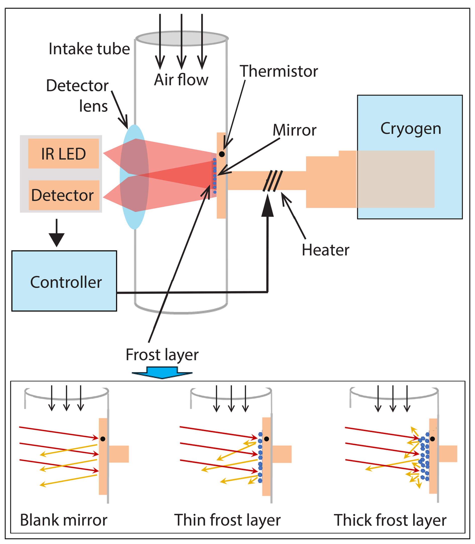
Figure 1 Frost point hygrometer and its various elements (not to scale). Top schematic: conceptual scheme (similar to Vömel et al., 2007a, and Hurst et al., 2023). A photodetector measures the light reflected by the mirror (indicated by the voltage U_m) and is used to adjust the mirror temperature (T_m) within a feedback loop by adjusting the current through a heater coil, which diminishes the continuous cooling of the mirror by the evaporating cryogen (R23). A digital microcontroller manages this feedback loop, so that the mirror can be rapidly heated and cooled to bring its temperature as close as possible to the instantaneous frost point (T_fp). Bottom inserts illustrate qualitatively how deposit on the mirror increases optical turbidity, thereby reducing the measured specular reflectance.

Under “good conditions”, i.e. for measurements with very stable PID control (the Proportional–Integral–Derivative controller used to regulate the mirror temperature), the total frost point uncertainty at the instrument's 1 s resolution is given by the deviation of the mirror temperature T_m and the frost point T_fp, namely $|T_{\mathrm{m}}-T_{\mathrm{fp}}|$ < 0.2 K (Fahey et al., 2014; Vömel et al., 2016). However, under rapidly changing conditions, the resulting controller oscillations can be well in excess of 0.2 K. Traditionally, the oscillations are smoothed out through time averaging. For example, for CFH a 25 s boxcar filter was used (corresponding to a vertical resolution of ∼ 125 m), and for FPH a 50 s boxcar filter (∼ 250 m), resulting in a total uncertainty of the average frost point of typically $|{\stackrel{\mathrm{‾}}{T}}_{\mathrm{m}}-{\stackrel{\mathrm{‾}}{T}}_{\mathrm{fp}}|$ < 0.51 K (Vömel et al., 2007a; Hall et al., 2016).

2.4 CFH feedback control and controller stability

CFH uses a digital PID controller designed for fast response during ascent (Vömel et al., 2007a). The control (or “manipulated”) variable is the heating power (as a fraction of the maximum 12 W) applied to the heater coil wound around the mirror stem. This results in a change in mirror temperature through Joule heating of the cryogenically cooled cold finger. The process (or “feedback”) variable is the specular reflectance U_m of the mirror (with setpoint 2.5 V corresponding to 88 % specular reflection). The mirror temperature T_m is the measurement output (in K), from which the amount of H₂O in the ambient gas phase is then derived. The feedback controller aims to maintain constant thickness of the condensate, which implies thermodynamic equilibrium with the gas phase (Barrett and Herndon, 1951; Mastenbrook and Oltmans, 1983). Assuming no instrumental problems, on a single measurement profile, the largest source of uncertainty is not the mirror temperature, but frost control stability (Vömel et al., 2016; Hall et al., 2016), which we describe and quantify in this work as nonequilibrium error. It can range from < 0.1 K during stable frost control to a few K in case of unstable frost control (Vömel et al., 2016; see also Fig. 7).

For long time series consisting of measurements from multiple balloon flights that have been downsampled to a coarse vertical resolution (e.g. for satellite comparison at a given pressure level as in Hurst et al., 2016), the error introduced by the controller oscillations is considered to be random (Vömel et al., 2016). During a single balloon flight, however, the frost point measurements (reported at 1 s resolution in the telemetry) are not randomly distributed around the true value, but exhibit some autocorrelation due to the oscillatory behavior of the PID controller (Vömel et al., 2016). Put simply, the reported mirror temperature periodically alternates between “swings” that are too warm or too cold. The period and amplitude of the oscillations depend on the controller's response to the transient dynamics of frost formation and evaporation, whose time scale is primarily governed by the difference between the ambient H₂O partial pressure and the ice vapor pressure (kinetic time scale ${\mathit{\tau }}_{\mathrm{kin}}\sim p/\mathrm{\Delta }{p}_{{\mathrm{H}}_{\mathrm{2}}\mathrm{O}}$). Further, it depends on the cryogen and ambient air temperatures, on the ventilation, and on the morphology of the frost coverage. This difficulty is only partially remedied by taking mean values of atmospheric layers, e.g. several 100 m thick, as done by Vömel et al. (2007a, 2016) and Hall et al. (2016).

2.5 CFH mirror temperature accuracy

CFH uses a small bead thermistor embedded into a gold-plated copper mirror disk of 7 mm diameter and 1.27 mm thickness, whose calibration is traceable to NIST (Vömel et al., 2007a). Details on the calibration procedure, accuracy and long-term stability are provided by Vömel et al. (2007a, 2016), see also Hall et al. (2016). We note that all CFH instruments analyzed in this work (Table A1) have serial numbers > 2L2825, such that a mirror temperature bias (see Vömel et al., 2016) is not expected. Adding all components in quadrature, the mirror temperature uncertainty is < 0.11 K for ice films and < 0.20 K for liquid films, as the random uncertainty of the thermistor measurement is largest in the lower troposphere and negligible higher up (Vömel et al., 2016; see also Hall et al., 2016). The systematic error, i.e. the error component that cannot be reduced by averaging over multiple measurements, is estimated to be less than 0.11 K (Vömel et al., 2016), and its main component is the inhomogeneity of the temperature across the mirror, reported to be less than 0.1 K (Oltmans, 1985; Vömel et al., 2007a; Hall et al., 2016). For routine measurements, it is good practice to perform a ground check before each launch (Immler et al., 2010; Vömel et al., 2016).

With a stable PID control, i.e. close to thermodynamic equilibrium between condensate and vapor phase, the accuracy of the CFH dew point or frost point is therefore excellent, with an overall uncertainty of < 0.2 K for ice and < 0.3 K for liquid condensate. This corresponds to an error in the H₂O mixing ratio of < 4 % up to the middle stratosphere (∼ 28 km), including the 0.3 hPa uncertainty of the RS41 radiosonde GPS-based pressure measurement (Vaisala, 2018b). This is also the basis for the temperature accuracy at the Golden Points presented in the next section. At the Golden Points all the oscillatory errors due to the PID controller, i.e. the main uncertainty of CFH, vanish. However, it is important to note that the accuracy of the frost point measurement depends not only on the instrument accuracy, but also on how well the position of a Golden Point along a profile is determined, which is particularly important for instruments with large amplitudes in the controller oscillations (see example in Sect. 5.7).

3 The Golden Points of chilled mirror hygrometry

In a Royal Society Bakerian Lecture in 1945, Dobson et al. (1946) described a chilled mirror hygrometer for accurately determining the frost point. In practice, for their “eye-observation” instrument, they observed the two temperatures at which the condensate “just increases” and “just decreases”, and then calculated the mean of these temperatures as being “very near the true frost-point”. This sandwiching of the equilibrium is essentially the Golden Point method. They further noted that, given the low temperatures in the UT/LS and the corresponding low H₂O vapor pressures, the growth/shrinking of the frost is a slow process. They wrote that this method is more accurate than the classic visual inspection of the dew point method (dating back to Daniell, 1820), where the temperature is measured when the condensate first appears and then completely disappears. This is because frost occurs only after the surface has cooled to 2–3 K below the frost point, i.e., frost formation requires massive supersaturation, which usually first leads to the formation of supercooled dew, from which the ice then nucleates.

3.1 Definition of Golden Points

Manual operation and visual detection have since been replaced by automatic sensitive measurements with photo-electric detection of frost on a mirror and a mirror temperature control loop, but the fundamental principle of chilled mirror hygrometry remained the same: when the condensate grows, its temperature is too low, when it shrinks, its temperature is too high. A modern frost point hygrometer attempts to automatically control the cooling power of its mirror such that the condensate neither grows nor shrinks (Barrett and Herndon, 1951; Mastenbrook and Oltmans, 1983). However, in order to stabilize the condensate under rapidly changing conditions during a balloon sounding, the instrument must regularly overshoot and undershoot the frost point by oscillations in the mirror temperature. In a stable laboratory environment and with a well-tuned feedback controller, small perturbations may lead to controller oscillations that decrease over time and may reach final amplitudes of only a few milli-Kelvin.

While errors smaller than 0.1 K can also be achieved during balloon soundings, they may reach several K and not be symmetric about the frost point due to the difference in frost formation and evaporation (Vömel et al., 2016). A chilled mirror hygrometer is therefore unable to maintain the condensate in a continuous (or static) equilibrium with the partial pressure of H₂O in the ambient air ($p_{{\mathrm{H}}_{\mathrm{2}}\mathrm{O}}$). Instead, the condensate undergoes intermittently moments in which the net exchange of water molecules with the gas phase vanishes. This occurs precisely when the condensate changes from growth to evaporation or vice versa, which corresponds to an extreme value in condensate thickness and, thus, in the mirror reflectance voltage U_m. In such an equilibrium-like moment, the net flux of H₂O is zero because the vapor pressure of the condensate and the H₂O partial pressure are equal ($p_{\mathrm{vap}}=p_{{\mathrm{H}}_{\mathrm{2}}\mathrm{O}}$). Therefore, only at these points does the chilled mirror hygrometer measure the true frost point.

For the sake of simplicity, in this article we refer to these equilibrium-like moments simply as “equilibrium,” even though the state with $p_{\mathrm{vap}}=p_{{\mathrm{H}}_{\mathrm{2}}\mathrm{O}}$ may only last for a fraction of a second. Specifically, all measurements with a net H₂O flux of zero between condensate and gas phase are referred to as the “Golden Points” of chilled mirror hygrometers. Formally, the relationship for the Golden Points reads

$$\begin{array}{}\text{(1)}& T_{\mathrm{m}}=T_{\mathrm{fp}}\iff {\displaystyle \frac{\mathrm{d}{U}_{\mathrm{m}}}{\mathrm{d}t}}=\mathrm{0}\end{array}$$

where T_m is the mirror temperature (an accurate representation of the condensate temperature), T_fp is the frost point of the ambient air, t is the time, U_m is the feedback variable for the amount of condensate, and $\mathrm{d}{U}_{\mathrm{m}}/\mathrm{d}t$ is the measure of condensate growth. In the case of CFH, U_m is the mirror reflectance given by the voltage of the photodetector (in V), which in turn controls the mirror temperature T_m. We call Eq. (1) the “Golden Points equation”.

Golden Points occur in all chilled mirror hygrometer measurements, regardless of whether they are cooled cryogenically (e.g. Mastenbrook and Oltmans, 1983) or thermo-electrically (e.g. Fujiwara et al., 2003; Sugidachi et al., 2025), or whether their feedback measurement for condensate growth is specular reflectance (e.g. Vömel et al., 2007a), light scattering (e.g. Brewer and Dobson, 1951), phase/frequency shifts of a surface acoustic wave (e.g. Hansford et al., 2006) or energy attenuation of alpha radiation (e.g. Rohrbough et al., 1967). Automatic chilled mirror hygrometers usually try to maintain their feedback variable U_m as close as possible to a predefined “setpoint” U_set, which is determined by a constant reflectance chosen to avoid a sudden loss of condensate while preserving good sensitivity to changes in condensate thickness. The effect of the feedback controller could lead to the misconception that U_m=U_set is a sufficient condition for equilibrium, i.e. T_m=T_fp. This is generally not true, as T_m=T_fp applies if and only if $\mathrm{d}{U}_{\mathrm{m}}/\mathrm{d}t$ = 0, which can occur far from the setpoint. Consequently, good chilled mirror instruments should have an optically sensitive ice film and measure mirror temperature and mirror reflectance simultaneously at high frequency, high accuracy, low noise and low reflex sensor drift. This is because excellent accuracy of the frost point measurement can only be achieved if the position of the Golden Point along the balloon trajectory is also precisely determined with well-synchronized temperature and reflectance time series. The accuracy is therefore not determined solely by the precision of the temperature sensor, but also by the accuracy of the position of the Golden Point. To meet the low noise condition, smoothing is often required. This concerns white noise from the electronics (on CFH, pre-launch clean mirror data indicates it contributes 10 % to the overall noise) and from the condensate itself (such as specular reflections of individual crystal faces), but above all spectral noise from problematic and unwanted signals that correspond to some eigenfrequency of the condensate-substrate-electronics system. In Fig. D1 we show that CFH with ice film sometimes appears to develop an eigenperiod of ∼ 5 s, which is not an atmospheric signal but needs to be removed by an appropriate smoothing. In this work we apply a smoothing of the CFH reflectance signal of 3 s for the liquid films and 15 s for the ice films (which takes account of changes in condensation rate and film morphology). Figures D1 and D2 suggest that a smoothing interval of 15 s is the optimal compromise between removing instrument artifacts and preserving natural features in the upper-air H₂O profile, and we examine the effects of using shorter or longer smoothing intervals. Smoothing complicates the determination of the exact timing of the Golden Point and must therefore be applied with caution in order not to reduce the accuracy of the frost point T_fp.

Reporting the Golden Points to achieve maximum accuracy is not new: the first accurate measurements of stratospheric water vapor performed by Dobson et al. (1946) were essentially the Golden Points of their manually operated hygrometer. In this respect, to our knowledge, they are the inventors of the Golden Points method. In the age of fully automated chilled mirror hygrometers, however, the method and its benefits fell into oblivion.

3.2 Application of the Golden Points method

A first example of using the Golden Points method is shown in Fig. 2, which compares the humidity measurements in the midlatitude tropopause region of three instruments: the CFH chilled mirror, the FLASH-B Ly-α fluorescence instrument and the thin-film humidity sensor of the RS41 radiosonde. Measuring the fine structure of UT/LS water vapor mixing ratio (on a scale < 100 m) with high accuracy (< 10 %) is still a challenge even for state-of-the-art instruments, especially around the tropopause, where an abrupt transition from moist tropospheric air to very dry stratospheric air takes place. Near the tropopause, the differences between the instruments shown in Fig. 2 are more than 30 % in H₂O mixing ratio, which is far from the target of < 4 % set by CIMO, let alone the target of 2 % set by GCOS. We show in this section that we can reduce these discrepancies to < 15 % when applying physically meaningful corrections to the thin-film and Ly-α instruments, based on the Golden Points of the chilled mirror instrument. As we will show in Sect. 5.2, we can further reduce the discrepancies to ∼ 5 %, when CFH controller instabilities leading to strong nonequilibrium states of the mirror are corrected by means of a nonequilibrium correction of CFH.

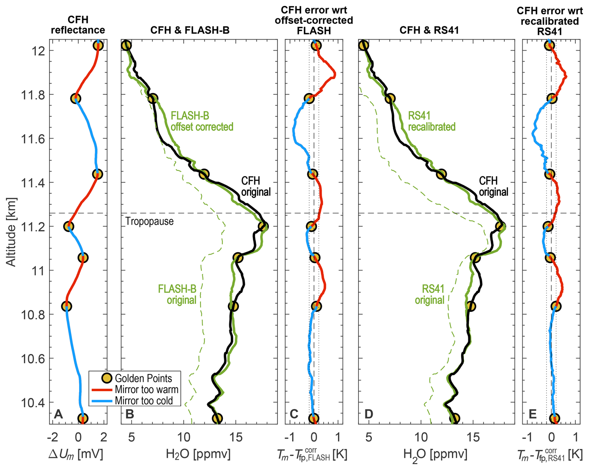
Figure 2 Sounding of the tropopause region over Lindenberg, eastern Germany, on 13 March 2017, 22:54 UT. Humidity was measured by three hygrometers on the same payload: CFH chilled mirror, FLASH-B Ly-α fluorescence instrument, and the thin-film polymer sensor of the RS41 radiosonde. (A) Mirror reflex signal (detector voltage U_m−U_set in mV) with the Golden Points located at the extreme values, where $\mathrm{d}{U}_{\mathrm{m}}/\mathrm{d}t$ = 0. (B) Original data of CFH (thick black curve) and FLASH-B (thin dashed green curve) as well as offset-corrected FLASH-B data (thick green curve), smoothed with the same ±10 s boxcar filter as the RS41 data. (C) Error of CFH frost point data with respect to the offset-corrected FLASH-B. (D) Original data of CFH (thick black curve, same as in panel B) and RS41 (thin dashed green curve) as well as time-lag and bias-corrected RS41 data (thick green curve). (E) Error of CFH frost point data with respect to the time-lag and bias-corrected RS41.

Figure 2B and D show the original data of the three instruments as thick black lines for CFH and as green dashed lines for the other two instruments. Both FLASH-B and RS41 suggest a much drier upper troposphere and lower stratosphere than CFH. However, the extreme values of CFH mirror reflectance ($\mathrm{d}{U}_{\mathrm{m}}/\mathrm{d}t$ = 0) indicate seven Golden Points in the selected altitude range, whose altitudes can be determined with sufficient accuracy (within better than ±5 m). CFH has been shown to measure the frost point with less than 0.2 K error under equilibrium conditions in the laboratory (Fahey et al., 2014) and under good flight conditions (Vömel et al., 2016), which we assume to also apply to the equilibrium situation of the Golden Points (see further Sect. 5.5 for a discussion of the uncertainty at the Golden Points). This corresponds to an uncertainty in the water vapor mixing ratio at frost point temperatures around 205 K and a pressure around 200 hPa of less than 0.5 ppmv (or 3 % in mixing ratio). Deviations in the original data of the other two instruments of several ppmv as shown in Fig. 2 therefore exceed the uncertainty at the Golden Points by almost an order of magnitude.

FLASH-B usually requires recalibration between flights. As Fig. 2 shows, large residual errors may be related to a constant offset in the fluorescence counts. Here, we determine the size of this offset from the CFH Golden Points. The FLASH-B instrument (“FI05/12”) in Fig. 2B can be corrected to match the Golden Points by assuming a constant offset (78.5 counts s⁻¹) in the fluorescence count rate (compared to typical count rates in the tropopause region of several hundred counts s⁻¹) prior to multiplication with the calibration constant (0.0256 ppmv (counts s⁻¹)⁻¹). This results in near-perfect agreement with the CFH water vapor mixing ratio at all seven Golden Points. See Appendix C for details on the FLASH-B offset.

RS41 typically requires corrections of the time-lag and bias of the thin polymer film measurement. In general, Vaisala's RS41 product, which is corrected for time lag but not for bias, shows good agreement with CFH in the lower and middle troposphere. Under the low relative humidities and low temperatures prevailing in the UT/LS, the RS41 generally still remains sensitive to moisture, but residual time-lag and bias errors, along with increasing sonde-to-sonde variability, reduce the accuracy of the RS41 measurement (Brunamonti et al., 2019; Poltera, 2022; see also Fig. B1 in Appendix B). Once the relative humidity above the tropopause drops below about 2 %RH, i.e., typically 1–3 km above the tropopause in midlatitudes, the RS41 lacks responsiveness to humidity changes (Survo et al., 2015; Vömel et al, 2022) and cannot be used as tandem hygrometer anymore. We apply our own processing to Vaisala raw data at the heated humidity sensor temperature (the Vaisala software provides the raw RH and T, at both sensor and air temperatures) by performing the following steps (see Sect. 4.2 and Appendix B for details):

• we apply a time-lag correction to the raw data of relative humidity from RS41 according to Miloshevich et al. (2004), using a 2-parameter fit for a time constant of Arrhenius type (see Eq. B1);

• we smooth the time-lag corrected data with a boxcar filter (in this case with a full width of ±10 s corresponding to about ±50 m in altitude);

• we apply a bias correction using a 6-parameter fit that minimizes the root mean square error (RMSE) between the frost points determined from the time-lag corrected and smoothed RS41 data and the CFH Golden Points (see Eq. B2).

This procedure shifts the RS41 data from the profile originally provided by the Vaisala software (green dashed curve in Fig. 2D) to the time-lag and bias corrected profile (green solid curve in Fig. 2D). Thereafter, at the Golden Points the remaining error between the corrected RS41 and CFH frost points remains below ±0.2 K (vertical dotted lines in Fig. 2E).

While the agreement between CFH on the one hand and the offset-corrected FLASH-B or the time-lag and bias-corrected RS41 on the other hand is excellent at the Golden Points, there are still discrepancies up to ±0.9 K away from the Golden Points (blue and red lines in Fig. 2C, E). These remaining discrepancies are due to the CFH controller oscillations. As we will show in the next section, they can be further decreased to ±0.4 K by applying a nonequilibrium correction to the CFH data.

4 Reflectance-based nonequilibrium correction away from the Golden Points

This section presents details on the nonequilibrium correction, first introduced by Poltera et al. (2021). By adjusting the mirror temperature, T_m, chilled mirror hygrometers aim at establishing equilibrium between the H₂O partial pressure in the ambient air and the H₂O vapor pressure of the condensate (frost or dew). The vapor pressure satisfies the Clausius-Clapeyron equation $\mathrm{d}{p}_{\mathrm{vap}}/p_{\mathrm{vap}}=\mathrm{\Delta }{H}_{\mathrm{vap}}/R\cdot \mathrm{d}T/T^{\mathrm{2}}$, where ΔH_vap denotes the heat of evaporation (≈ 51 kJ mol⁻¹ for ice) and R the universal gas constant. For constant ΔH_vap, the Clausius-Clapeyron equation has the Arrhenius-type solution $p_{\mathrm{vap}}\propto \exp (-\mathrm{\Delta }{H}_{\mathrm{vap}}/RT)$.

4.1 Quantifying the nonequilibrium

Under nonequilibrium conditions, if the mirror is too cold, the net H₂O flux towards the mirror is positive, the condensate grows, and the mirror reflectance decreases (T_m < T_fp ⇒ $\mathrm{d}{U}_{\mathrm{m}}/\mathrm{d}t$ < 0), and vice versa for too warm conditions. Determining equilibrium according to Eq. (1) is straightforward, but is only a consequence of a more general nonequilibrium equation. Quantifying nonequilibrium relies on three assumptions, which we describe in the following subsections.

4.1.1 Assumption I: mirror reflectance responds linearly to H₂O flux changes

The relationship $U_{\mathrm{m}}(M_{{\mathrm{H}}_{\mathrm{2}}\mathrm{O}}$) between the amount of specularly reflected light given by the voltage U_m (in V) and the amount of condensate on the mirror $M_{{\mathrm{H}}_{\mathrm{2}}\mathrm{O}}$ (in mol m⁻²) is a monotonically decreasing function. We assume that the relationship is linear over a small range of mirror reflectances around the setpoint U_set (Barrett and Herndon, 1951):

$$\begin{array}{}\text{(2)}& {\displaystyle \frac{\mathrm{d}{U}_{\mathrm{m}}}{\mathrm{d}t}}={\displaystyle \frac{\mathrm{d}{U}_{\mathrm{m}}}{\mathrm{d}{M}_{{\mathrm{H}}_{\mathrm{2}}\mathrm{O}}}}\cdot {\displaystyle \frac{\mathrm{d}{M}_{{\mathrm{H}}_{\mathrm{2}}\mathrm{O}}}{\mathrm{d}t}}\equiv -A\cdot {\displaystyle \frac{\mathrm{d}{M}_{{\mathrm{H}}_{\mathrm{2}}\mathrm{O}}}{\mathrm{d}t}}.\end{array}$$

We term $A^{\prime }=-\mathrm{d}{U}_{\mathrm{m}}/\mathrm{d}{M}_{{\mathrm{H}}_{\mathrm{2}}\mathrm{O}}$ the “morphological sensitivity” of the mirror condensate (in V (mol m⁻²)⁻¹), which depends on the morphology of the condensate, e.g. ice crystal size and shape. Under many circumstances, within a flight segment, A^′ is approximately constant. For CFH, we estimate that the linearity holds for $|U_{\mathrm{m}}-U_{\mathrm{set}}|$ < $U_{\mathrm{set}}/\mathrm{100}$ for ice condensates and $|U_{\mathrm{m}}-U_{\mathrm{set}}|$ < $U_{\mathrm{set}}/\mathrm{10}$ for liquid water condensates, with U_set = 2.5 V. The assumption that A^′ is constant means that the morphology of the condensate near the setpoint remains stable over time, whereas abrupt morphology changes, such as the tearing off of pieces of the ice film violate this assumption (i.e., measurements at and shortly after such an event are considered artifacts). A similar linear relationship near the setpoint is assumed for chilled mirror hygrometers using light scattering from the condensate instead of specular reflectance from the mirror as feedback variable, such as SKYDEW (Sugidachi et al., 2025).

4.1.2 Assumption II: net H₂O flux is diffusion-controlled

A thin layer of thickness Δx_diff, Prandtl's boundary layer, is located above the mirror and its condensate, in which molecular gas phase diffusivity determines the time scale of mass transfer between the flowing air and the condensate. It can be approximated as $\mathrm{\Delta }{x}_{\mathrm{diff}}=\mathrm{\Delta }{x}_{\mathrm{diff}}(L,\mathit{Re})\approx \frac{\mathrm{5}}{\mathrm{3}}L/{\mathit{Re}}^{\mathrm{1}/\mathrm{2}}$ (Schlichting and Gersten, 2017), where L = 3.5 mm is the distance from the mirror edge to its center. We further simplify this (using $\mathit{Re}=\mathit{\rho }/\mathit{\mu }\times \mathit{\upsilon }/L$, with the dynamic viscosity of air μ≈0.017 mPa s) to $\mathrm{\Delta }{x}_{\mathrm{diff}}\approx \mathrm{150}\mathrm{\mu }\mathrm{m}\times \left(\mathit{\rho }\right(\mathrm{0})/\mathit{\rho }(z){)}^{\mathrm{1}/\mathrm{2}}\times ({\mathit{\upsilon }}_{\mathrm{0}}/\mathit{\upsilon }{)}^{\mathrm{1}/\mathrm{2}}$, where ρ(z) is the air density at altitude z, ρ(0) ≈ 1.3 kg m⁻³, υ is the balloon vertical velocity and υ₀ = 5 m s⁻¹. For most of the applications within the upper troposphere, Δx_diff≈250 µm is a sufficient approximation. Fick (1855)'s first law for the H₂O molecular flux onto the mirror reads (Taylor and Krishna, 1993):

$$\begin{array}{}\text{(3)}& {\displaystyle \frac{\mathrm{d}{M}_{{\mathrm{H}}_{\mathrm{2}}\mathrm{O}}}{\mathrm{d}t}}={\displaystyle \frac{D_{{\mathrm{H}}_{\mathrm{2}}\mathrm{O}}\left(\stackrel{\mathrm{‾}}{p},\stackrel{\mathrm{‾}}{T}\right)}{\mathrm{\Delta }{x}_{\mathrm{diff}}\cdot R\stackrel{\mathrm{‾}}{T}}}\cdot \left(p_{{\mathrm{H}}_{\mathrm{2}}\mathrm{O}}-p_{\mathrm{vap}}\left(T_{\mathrm{ice}}\right)\right),\end{array}$$

where $\mathrm{d}{M}_{{\mathrm{H}}_{\mathrm{2}}\mathrm{O}}/\mathrm{d}t$ is the H₂O molar flux onto the mirror, $D_{{\mathrm{H}}_{\mathrm{2}}\mathrm{O}}$ is the diffusion coefficient of H₂O molecules in air (in m² s⁻¹), R is the ideal gas constant, Δx_diff is the boundary layer thickness, $p_{{\mathrm{H}}_{\mathrm{2}}\mathrm{O}}$ is the H₂O partial pressure in the ambient air and p_vap(T_ice) the H₂O vapor pressure of the ice film on the mirror with temperature T_ice, or of the liquid in the case of dew. Furthermore, $\stackrel{\mathrm{‾}}{p}$ and $\stackrel{\mathrm{‾}}{T}$ are the average pressure and temperature in the diffusion layer between the ice surface and the ambient air (Taylor and Krishna, 1993), taken here as $\stackrel{\mathrm{‾}}{p}\approx p_{\mathrm{air}}$ and $\stackrel{\mathrm{‾}}{T}\approx T_{\mathrm{air}}$. We approximate the gas phase diffusion coefficient of H₂O as $D_{{\mathrm{H}}_{\mathrm{2}}\mathrm{O}}(p,T)\approx D_{\mathrm{0}}\cdot (p_{\mathrm{0}}/p)\cdot (T/T_{\mathrm{0}}{)}^{\mathrm{2}}$, with the standard diffusion coefficient D₀ = 0.21 cm² s⁻¹, standard pressure p₀ = 1013 hPa and standard temperature T₀ = 273 K (Pruppacher and Klett, 2010). Finally, note that the H₂O partial pressure satisfies $p_{{\mathrm{H}}_{\mathrm{2}}\mathrm{O}}=p_{\mathrm{vap}}(T_{\mathrm{fp}}$).

4.1.3 Assumption III: mirror temperature equals condensate temperature

Finally, we assume that the measured mirror temperature T_m is an accurate representation of the condensate temperature T_ice with negligible time-lag:

$$\begin{array}{}\text{(4)}& T_{\mathrm{ice}}=T_{\mathrm{m}}.\end{array}$$

Vömel et al. (2016) estimated temperature inhomogeneities to be less than 0.1 K, owing to the high heat conductivity (about 400 W m⁻¹ K⁻¹) of the gold-plated copper mirror of CFH (Vömel et al., 2007a) and the only few micrometers thick ice crystals on the mirror (Leu and Keyser, 2009) after the CFH cleaning cycles at −15 °C dew point and −53 °C frost point. Convective heat transfer from the flowing air to the mirror is not negligible and must be taken into account in the implementation of the PID controller (Vömel and Jeannet, 2013). Nevertheless, the temperature of the mirror surface and the ice film equilibrate within ∼ 120 ms when the total heat load changes (assuming a characteristic length scale < 3.5 mm for the copper mirror disk and < 0.1 mm for the thin ice film). Therefore, inhomogeneities in the mirror temperature and uncertainties of the thermistor are covered by the overall mirror temperature uncertainty of at most 0.11 K (Vömel et al., 2016), as long as $\mathrm{d}{T}_{\mathrm{m}}/\mathrm{d}t\lesssim \mathrm{0.9}$ K s⁻¹, which most often holds for CFH.

4.1.4 The nonequilibrium equation

When the deviation from the mirror reflectance setpoint is sufficiently well constrained by the micro-controller, the change in mirror reflectance is proportional to the net flux of H₂O molecules with a timescale governed by diffusive transport in the thin layer over the mirror. Then, combining Eqs. (2)–(4) yields the “nonequilibrium equation”:

$$\begin{array}{}\text{(5)}& {\displaystyle \frac{\mathrm{d}{U}_{\mathrm{m}}}{\mathrm{d}t}}=A^{\prime }{\displaystyle \frac{D_{{\mathrm{H}}_{\mathrm{2}}\mathrm{O}}\left(\stackrel{\mathrm{‾}}{p},\stackrel{\mathrm{‾}}{T}\right)}{\mathrm{\Delta }{x}_{\mathrm{diff}}\cdot R\stackrel{\mathrm{‾}}{T}}}\cdot \left(p_{\mathrm{vap}}\left(T_{\mathrm{m}}\right)-p_{\mathrm{vap}}\left(T_{\mathrm{fp}}\right)\right).\end{array}$$

Equation (5) is the quantification of nonequilibrium conditions on the mirror. If and only if the mirror reflectance assumes an extreme value (i.e., a local maximum or minimum, $\mathrm{d}{U}_{\mathrm{m}}/\mathrm{d}t$ = 0), the mirror temperature is at the frost (dew) point (T_m=T_fp or T_dp) and the nonequilibrium vanishes, i.e., Eq. (5) relaxes to the Golden Point equation.

At the Golden Points, the mirror temperature is the most accurate estimate of the true atmospheric frost (dew) point within the sampling period of ±1 s. In contrast, between the Golden Points the mirror is in a nonequilibrium state. Equation (5) provides a fundamental mathematical relationship between mirror temperature and mirror reflectance:

• When the mirror reflectance increases ($\mathrm{d}{U}_{\mathrm{m}}/\mathrm{d}t$ > 0), the mirror coverage decreases, the condensate evaporates, the mirror is too warm (i.e. the mirror temperature experiences a warm “excursion”).

• When the mirror reflectance decreases ($\mathrm{d}{U}_{\mathrm{m}}/\mathrm{d}t$ < 0), the mirror coverage increases, the condensate grows, the mirror is too cold (i.e. the mirror temperature experiences a cold “excursion”).

• When the mirror reflectance passes through a minimum ($\mathrm{d}{U}_{\mathrm{m}}/\mathrm{d}t$ = 0, $d^{\mathrm{2}}{U}_{\mathrm{m}}/\mathrm{d}{t}^{\mathrm{2}}$ > 0), the condensate changes from growth to evaporation as the mirror temperature is crossing the frost (dew) point.

• When the mirror reflectance passes through a maximum ($\mathrm{d}{U}_{\mathrm{m}}/\mathrm{d}t$ = 0, $d^{\mathrm{2}}{U}_{\mathrm{m}}/\mathrm{d}{t}^{\mathrm{2}}$ < 0), the condensate changes from evaporation to growth as the mirror temperature is crossing the frost (dew) point.

• If the reflectance of the mirror remains almost constant ($\mathrm{d}{U}_{\mathrm{m}}/\mathrm{d}t$ ≈ 0, $d^{\mathrm{2}}{U}_{\mathrm{m}}/\mathrm{d}{t}^{\mathrm{2}}\approx \mathrm{0}$) and the quality of the ice film is good, the condensate neither grows nor evaporates rapidly, and the mirror temperature is close to the frost (dew) point; due to the permanently changing atmospheric conditions along the balloon trajectory, such mirror reflectance “plateaus” or “Golden Ranges” occur much less frequently than mirror reflectance oscillations.

During a balloon sounding, chilled mirror hygrometers with accurate mirror temperature sensors and reflectance measurements with good signal-to-noise ratio pass through a series of Golden Points with accurate T_fp measurements. The number of Golden Points depends on:

• the setting (or “tuning”) of the feedback controller (i.e., desired response speed to a sudden change in the frost point)

• the airflow through the inlet tube

• the morphology of the condensate (fine vs. coarse frost, as well as patchy vs. homogeneous frost distribution)

• the state of the atmosphere (slow vs. fast varying frost point).

For CFH, the temporal sequence of Golden Points typically ranges from a few seconds in the lower troposphere to a few tens of seconds in the UT/LS. As we will see in the case studies in Sect. 5, the Golden Points enable the in-situ/flight recalibration of other sensors flown in tandem with CFH, such as the RS41, which in turn allows applying a nonequilibrium correction to the CFH data.

4.1.5 Linearized form of the nonequilibrium correction

In order to improve applicability in control theory with the heat balance equation ($\mathrm{d}{T}_{\mathrm{m}}/\mathrm{d}t$ ∝ applied heat) and facilitate the use for frost point hygrometers, which measure temperatures, we rewrite the nonequilibrium equation (Eq. 5) by means of the linearized form of the Clausius-Clapeyron equation, $p_{\mathrm{vap}}\left(T_{\mathrm{m}}\right)-p_{\mathrm{vap}}\left(T_{\mathrm{fp}}\right)\approx \mathrm{\Delta }{H}_{\mathrm{vap}}/R\cdot p_{\mathrm{vap}}\left(T_{\mathrm{m}}\right)/T_{\mathrm{m}}^{\mathrm{2}}\cdot (T_{\mathrm{m}}-T_{\mathrm{fp}})$, valid for $|T_{\mathrm{m}}-T_{\mathrm{fp}}|$ smaller than 1–2 K, to obtain a linearization of $\mathrm{d}{U}_{\mathrm{m}}/\mathrm{d}t$ in terms of the temperature deviation:

$$\begin{array}{}\text{(6)}& {\displaystyle \frac{\mathrm{d}{U}_{\mathrm{m}}}{\mathrm{d}t}}\approx A^{\prime }\cdot {\displaystyle \frac{D_{{\mathrm{H}}_{\mathrm{2}}\mathrm{O}}\left(\stackrel{\mathrm{‾}}{p},\stackrel{\mathrm{‾}}{T}\right)}{\mathrm{\Delta }{x}_{\mathrm{diff}}\cdot R\stackrel{\mathrm{‾}}{T}}}\cdot {\displaystyle \frac{\mathrm{\Delta }{H}_{\mathrm{vap}}}{R}}\cdot {\displaystyle \frac{p_{\mathrm{vap}}\left(T_{\mathrm{m}}\right)}{T_{\mathrm{m}}^{\mathrm{2}}}}\cdot \left(T_{\mathrm{m}}-T_{\mathrm{fp}}\right).\end{array}$$

Once the morphological sensitivity, $A^{\prime }=-\mathrm{d}{U}_{\mathrm{m}}/\mathrm{d}{M}_{{\mathrm{H}}_{\mathrm{2}}\mathrm{O}}$, of the mirror condensate is known, Eq. (6) can be used to quantify the temperature error of the mirror, T_m−T_fp, as all the other terms in this equation are known physical constants or measured quantities. The least well-known quantity is the thickness of the boundary layer, which during balloon ascent in the upper troposphere is typically Δx_diff≈250 µm (see Sect. 4.1.2). However, Δx_diff can be thicker in situations of poor ventilation ($\mathrm{\Delta }{x}_{\mathrm{diff}}\propto {\mathit{\upsilon }}_{\mathrm{flow}}^{-\mathrm{1}/\mathrm{2}}$), such as under prelaunch conditions, or thinner in situations of strong ventilation, such as directly after the burst of the balloon.

We can rewrite Eq. (6) as

$$\begin{array}{}\text{(7)}& {\displaystyle \frac{\mathrm{d}{U}_{\mathrm{m}}}{\mathrm{d}t}}\approx A\cdot {\displaystyle \frac{\stackrel{\mathrm{‾}}{T}}{T_{\mathrm{m}}}}\cdot {\mathit{\chi }}_{{\mathrm{H}}_{\mathrm{2}}\mathrm{O}}\left(T_{\mathrm{m}}\right)\cdot {\displaystyle \frac{T_{\mathrm{m}}-T_{\mathrm{fp}}}{T_{\mathrm{m}}}},\end{array}$$

where A is the “effective sensitivity”, namely $A=A^{\prime }\cdot D_{\mathrm{0}}\cdot p_{\mathrm{0}}\cdot \mathrm{\Delta }H/(\mathrm{\Delta }{x}_{\mathrm{diff}}\cdot (R{T}_{\mathrm{0}}{)}^{\mathrm{2}})\approx A^{\prime }\cdot \mathrm{84}$ mol (m² s)⁻¹ in V s⁻¹. This parameter is assumed constant within a flight segment, and combines the morphological sensitivity A^′ (in V (mol m⁻²)⁻¹), the thickness of Prandtl's boundary layer (Δx_diff≈250 µm), the heat of evaporation of ice (ΔH_vap≈51 kJ mol⁻¹) and the universal gas constant (R = 8.3145 J (K mol)⁻¹). Furthermore, ${\mathit{\chi }}_{{\mathrm{H}}_{\mathrm{2}}\mathrm{O}}\left(T_{\mathrm{m}}\right)=p_{\mathrm{vap}}\left(T_{\mathrm{m}}\right)/\stackrel{\mathrm{‾}}{p}$ is the H₂O mixing ratio estimated from the mirror temperature. The correction of the mirror temperature is then easily written as

$$\begin{array}{}\text{(8a)}& T_{\mathrm{fp}}\left(t\right)\approx T_{\mathrm{m}}\left(t\right)-{\displaystyle \frac{B\left(t\right)}{A}}\cdot {\displaystyle \frac{\mathrm{d}{U}_{\mathrm{m}}}{\mathrm{d}t}}\left(t\right),\end{array}$$

where $B\left(t\right)=T_{\mathrm{m}}^{\mathrm{2}}/(\stackrel{\mathrm{‾}}{T}\cdot {\mathit{\chi }}_{{\mathrm{H}}_{\mathrm{2}}\mathrm{O}}(T_{\mathrm{m}}\left)\right)$ in K is a function of temperatures and of the water vapor mixing ratio.

Equation (8a) allows to perform a nonequilibrium correction of the CFH measurement between the Golden Points directly in terms of frost point, the primary measured quantity of frost point hygrometers. However, this requires knowledge of the morphological sensitivity $A^{\prime }=-\mathrm{d}{U}_{\mathrm{m}}/\mathrm{d}{M}_{{\mathrm{H}}_{\mathrm{2}}\mathrm{O}}$, which can differ by more than an order of magnitude from flight to flight and even changes after each CFH cleaning cycle (as shown in Sect. 6.1). Different A^′ reflect large variability in ice film morphology due to slightly different conditions at the time of ice nucleation and growth (and possibly sintering) on the mirror following the cleaning cycles. Therefore, obtaining A^′ typically requires measurements by a second, independent instrument on the same platform, such as RS41 or FLASH, to establish an in-flight nonequilibrium correction of CFH.

However, there are a number of causes of residual errors that are not corrected by the nonequilibrium correction, even when excluding measurements affected by contamination of the inlet tube by hydrometeors or outgassing of the balloon skin, or by strong electronic interference. Such residual errors include: (i) uncertainties in $\mathrm{d}{U}_{\mathrm{m}}/\mathrm{d}t$ due to stray light, which can be largely avoided by flying only at night; (ii) abrupt jumps in U_m due to break-off of parts of the ice film, deposition of cloud particles on the mirror, or the sudden onset of specular reflection of individual crystal faces, all of which occur very rarely, and are typically flagged and discarded in the NDACC CFH processing (Vömel et al., 2016, their Appendix A); (iii) an uncertainty in A due to a lack of responsiveness of the second sensor to humidity changes, which is regularly the case for RS41 when the relative humidity above the tropopause drops below 2 %RH, so that the correction of CFH in the stratosphere must rely on the sensitivity A determined for the second ice film in the upper troposphere. While point (iii) may appear to be a major drawback in using RS41-derived sensitivities A to correct CFH in the stratosphere, this work will show below that Aderived in the upper troposphere can be used very well deep in the stratosphere (provided the thickness of the Prandtl Boundary layer, Δx_diff, is adapted appropriately, see Sect. 5.6.1).

4.2 Using auxiliary sensors for the nonequilibrium correction of CFH

Throughout the troposphere and stratosphere, the CFH measurements are excellent at the Golden Points, i.e. T_fp accurate to ±0.2 K, corresponding to errors in H₂O vapor pressure or mixing ratio of less than 3.5 % (except where measurements are contaminated; Jorge et al., 2021). By contrast, nonequilibrium states of the controller may cause much larger errors just a few meters above or below the Golden Points. Realizing the CIMO and GCOS goals requires measurements of the atmospheric frost point with low uncertainty and high vertical resolution. For this, we need to correct the nonequilibrium errors between the Golden Points, which can be achieved by a second sensor on the same payload after recalibrating it using the Golden Points. This could be a sensor with higher vertical resolution than the Golden Points, but with lower accuracy than CFH. Sensors with sufficient capabilities include the humidity sensor of the RS41 or the FLASH-B hygrometer, while certain other sondes may not be suitable, because of a slow response in the upper troposphere and insufficient stratospheric RH sensitivity, such as the often-used iMet-1 radiosonde (e.g. Hurst et al., 2011b). As we will discuss in Sect. 4.3, under certain circumstances, correction can be achieved without the help of other sensors, i.e. by means of a self-correction of the frost point hygrometer. However, this is usually not possible when Golden Points are far apart. Instead, another well-calibrated sensor is needed to correct the measurement errors.

In Sect. 5.1 and 5.2, we present case studies of nonequilibrium correction with the auxiliary sensors RS41 and FLASH-B. The corresponding correction methodologies of RS41 and FLASH-B by means of the CFH Golden Points are described in Appendices B and C respectively.

Using an auxiliary sensor for this purpose, we apply the nonequilibrium correction according to the following scheme:

• identify the Golden Points along the humidity profile measured by a chilled mirror instrument;

• construct an a-priori estimate of the frost point profile by means of an auxiliary sensor on the same balloon payload, which is corrected by means of the Golden Points of the chilled mirror instrument;

• use this a-priori estimate to determine the effective sensitivity A;

• construct an a-posteriori by correcting the CFH mirror temperature using A in Eq. (8a), called “nonequilibrium corrected CFH”.

The a-posteriori is our best approximation for the frost point. We use the deviation between the a-priori and the a-posteriori as an estimate of the uncertainty of the frost point resulting from residual errors in the nonequilibrium correction of CFH and the correction of the auxiliary sensor data based on the CFH Golden Points. For the details of time-lag and bias correction of each flight section using the CFH Golden Points see Appendix B. The details of offset correction for FLASH-B are given in Appendix C.

The effective sensitivity A can then be determined from a least squares fit using the scaled time derivative of the mirror reflectance $B\cdot \mathrm{d}{U}_{\mathrm{m}}/\mathrm{d}t$ as function of the difference of corrected auxiliary sensor data, $T_{\mathrm{fp},\mathrm{aux}}^{\mathrm{corr}}$ and the CFH mirror temperature T_m:

$$\begin{array}{}\text{(8b)}& B\cdot {\displaystyle \frac{\mathrm{d}{U}_{\mathrm{m}}}{\mathrm{d}t}}\approx A\cdot \left(T_{\mathrm{m}}-T_{\mathrm{fp},\mathrm{aux}}^{\mathrm{corr}}\right).\end{array}$$

Note that Eq. (8b) is equivalent to Eq. (8a), but with the still unknown true frost point T_fp approximated by the known corrected auxiliary sensor ($T_{\mathrm{fp},\mathrm{aux}}^{\mathrm{corr}}$). Figure 3D below shows a textbook example of the determination of A immediately before the launch of a balloon sonde using RS41 as auxiliary sensor (for the liquid film, i.e. with $T_{\mathrm{dp},\mathrm{RS}\mathrm{41}}^{\mathrm{corr}}$ instead $T_{\mathrm{fp},\mathrm{aux}}^{\mathrm{corr}}$), resulting in A = 773 V s⁻¹. In Sect. 6, we estimated A in flight for 70 soundings from the tropics to the polar regions, and found for the liquid film and the first and second ice films a median value of A≈6000 V s⁻¹, albeit with a high degree of variability (700–34 000 V s⁻¹, see Fig. 11). An effective sensitivity of 6000 V s⁻¹ is an average value for a good ice film and translates to a morphological sensitivity A^′ ≈ 71.4 V (mol m⁻²)⁻¹ ≈ 40 µV (ng cm⁻²)⁻¹ under typical balloon ascent ventilation conditions. With detectable changes (at $S/N$ = 2) in CFH reflectance of about 20 µV s⁻¹ during nighttime flights, this means (using Eq. 8a with B = 3 × 10⁷ K and $\mathrm{d}{U}_{\mathrm{m}}/\mathrm{d}t$ = 20 µV s⁻¹) that CFH can achieve measurements with a precision of 0.1 K in frost point or 100 ppbv H₂O in the lower stratosphere at 1 s temporal resolution (or 40 ppbv at 5 s resolution).

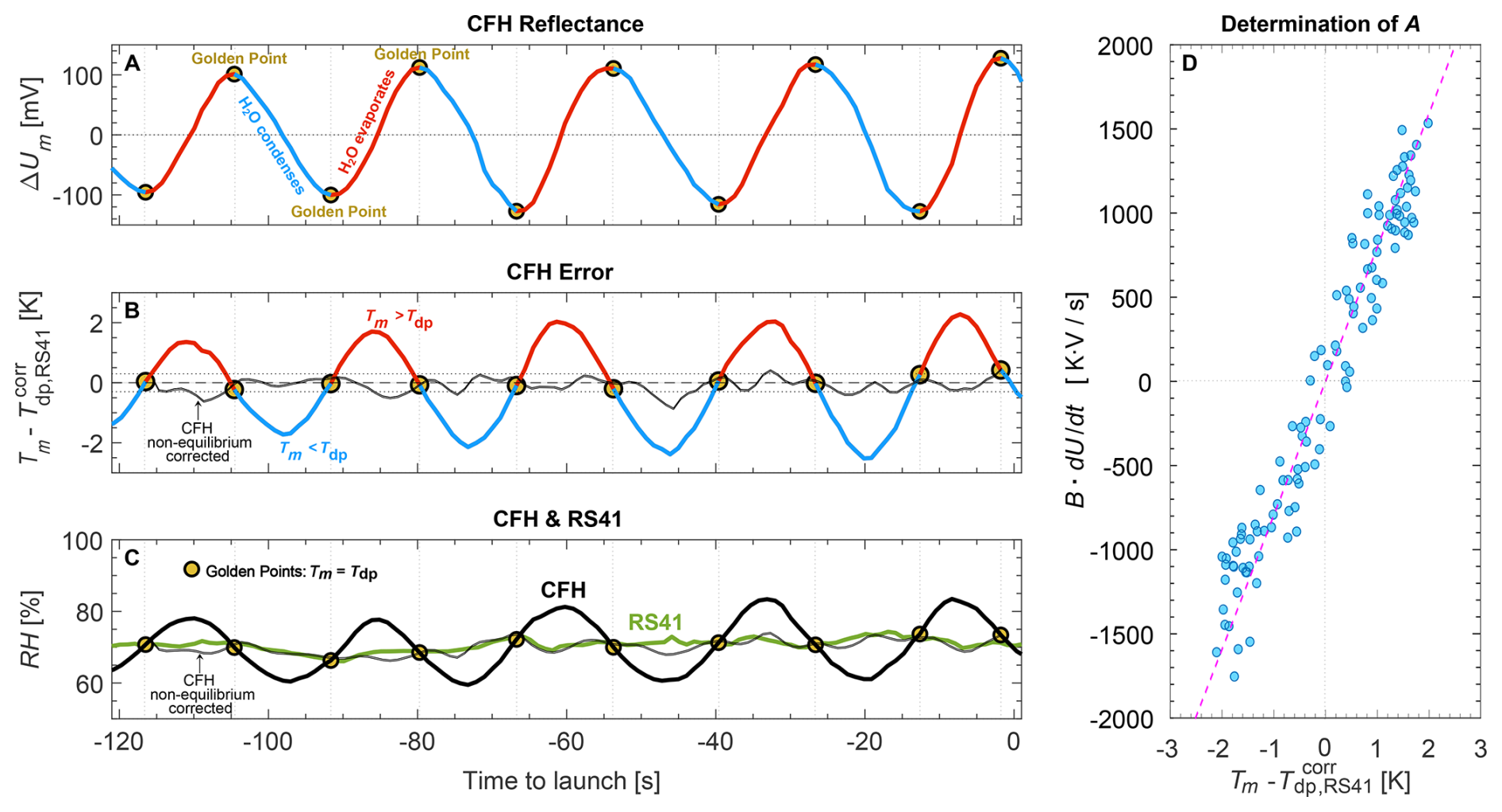
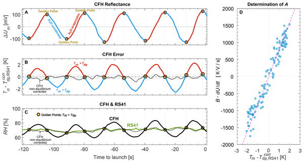
Figure 3 Nonequilibrium correction applied to prelaunch measurements of CFH and RS41 before the sounding in Lindenberg on 13 March 2017. (A) CFH mirror reflectance deviation from setpoint $\mathrm{\Delta }{U}_{\mathrm{m}}=U_{\mathrm{m}}-\mathrm{2.5}$ V. Color coding: red where reflectance increases as the condensate evaporates, blue where reflectance decreases as the condensate grows. Circles: Golden Points, where the reflectance reaches an extreme value as the condensate reaches equilibrium with ambient air. (B) Nonequilibrium error of CFH, i.e., difference between mirror temperature T_m and the dew point from RS41 (in K). Horizontal dotted lines at ±0.3 K: 2σ accuracy that we assert for the Golden Points of the CFH instrument when the coverage on the mirror is liquid dew instead of solid frost (i.e., in the lower troposphere). (C) Green line: RH (in %) from Vaisala's RS41 output. Thick black line: RH from CFH calculated using CFH mirror temperature T_m and air temperature (4.3 °C, measured by RS41). Circles: Golden Points indicating the times when CFH mirror temperature is at the dew point. Thin black lines in panels (B) and (C): RH from CFH corrected for nonequilibrium errors according to Eq. (8b) (without correction of RS41). (D) Scatter plot of the scaled time derivative of CFH mirror reflectance $B\cdot \mathrm{d}{U}_{\mathrm{m}}/\mathrm{d}t$ (see Eq. 8b) versus the difference of the CFH mirror temperature and the dew point derived from the RS41 measurement (blue circles). Magenta line: fitted effective sensitivity A = 773 V s⁻¹.

4.3 Nonequilibrium correction of CFH without other sensors

In addition to using a second instrument for non-equilibrium correction, there are other options. These are based on the fact that, for a given ice film, a reference between (at least two) Golden Points is required in order to evaluate the sensitivity parameter A of the ice film and then perform the nonequilibrium correction. These options are:

• Use of the self-correction of the chilled mirror instrument when descent data of good quality are available in addition to ascent data, to identify features in humidity in the uppermost kilometers of a sounding. See example in Sect. 5.3.

• Use of extreme conditions, such as after the Hunga Tonga eruption, where CFH shows large nonequilibrium deviations: precise a-priori H₂O mixing ratios between the enhanced plume regions that the optical backscatter sonde COBALD helped to identify are not of great importance compared to the benefits of applying the nonequilibrium correction. See example in Sect. 5.6.2.

However, these possibilities are only applicable to particular circumstances. Another option with general applicability is to modify the feedback controller of the chilled mirror instrument in order to obtain more closely spaced Golden Points. This may relax the requirement for an external reference and enable a nonequilibrium self-correction. This is the case with the recent development of SKYDEW (Sugidachi et al., 2025), see Sect. 5.7. The SKYDEW (FW v1.0) data product, which is based only on the Golden Points, has a vertical resolution of 150–250 m, whereas a higher vertical resolution (< 50 m) and similar accuracy (< 0.5 K) could be achieved with a proper nonequilibrium correction.

5 Nonequilibrium correction under various conditions

We illustrate the application of the nonequilibrium correction using case studies that represent different situations during a balloon sounding: prelaunch or “laboratory-like” conditions in a static atmosphere, measurements in the UT/LS in a dynamic atmosphere, and comparing ascent and descent data to validate measurements in the stratosphere. These case studies demonstrate that

• crossing the controller setpoint, i.e. the preset reflectance value, does not imply that the condensate is in equilibrium with the gas phase, but only that the condensate has the predefined thickness at this instant;

• chilled mirror instruments do not exhibit a first-order time-lagged response, so that the concept of an e-folding time constant is not appropriate;

• smoothing the mirror temperature or mixing ratio with a low-pass filter and using the residuals as an estimate for the controller error does not always provide an accurate representation of the measurement uncertainty.

Not all instruments or flight segments suffer from nonequilibrium errors to the same extent. While the nonequilibrium errors of some soundings are less than 0.1 K (an example is shown in Fig. 7A), so that the total uncertainty of the frost point measurement at 1 s resolution (including the uncertainty of the mirror calibration) is better than 0.2 K, for other soundings the nonequilibrium errors can reach several degrees Kelvin for hundreds of meters, so that the conventional technique of segment-wise averaging does not allow to retrieve the frost point if no correction of the nonequilibrium error is applied (see Sect. 5.4 on low-pass filtering).

5.1 Nonequilibrium correction under prelaunch conditions

Figure 3 shows CFH prelaunch data in outside air shortly before the balloon was released. During prelaunch, a small fan is temporarily installed on the upper inlet tube (Vömel et al., 2016), but the ventilation it creates is less than the airflow during the balloon ascent, resulting in pronounced oscillations in the CFH measurement. At the Golden Points, CFH compares well with the humidity measured by RS41 (after applying a 3.5 s synchronization shift Δ_tele discussed in Appendix B). In this example with a nearly constant ambient dew point, the strong oscillations observed in the signal are caused by mirror temperature oscillations resulting from a controller instability, i.e., “nonequilibrium excursions”, and not by a time-lagged response to changes in the dew point. In this special case without external dew point changes, the nonequilibrium errors in mirror temperature are nearly symmetric, but with a slight negative bias due to the nonlinearity of the Clausius-Clapeyron equation. If, instead of nonequilibrium correction, the H₂O mixing ratio or relative humidity is averaged over two periods (e.g., Vömel et al., 2007b), this would provide an accurate representation of the dew point, but the temporal resolution would still be about three times coarser than the Golden Points sampled with Eq. (1). A proper nonequilibrium correction using Eq. (8a) further increases the temporal resolution (here by a factor of 3 compared to using solely the Golden Points), enabling dew/frost point retrievals with similar measurement uncertainty but higher temporal resolution. The relative humidity of the nonequilibrium-corrected CFH agrees well with RS41; some residual differences might be due to both instruments actually measuring slightly different air due to small disturbances caused by the handling of the payload during the launching procedure.

Figure 3 illustrates that when the reflectance passes through the setpoint, this does not indicate that thermodynamic equilibrium is attained as discussed in Sect. 3. For example, the reflectance is at the setpoint at t = −20 s, yet the mirror temperature is at maximum distance from the dew point. Thermodynamic equilibrium is only reached when the reflectance remains constant or when it reaches a minimum or a maximum (e.g., at t = −40 s).

Figure 3D shows how the nonequilibrium correction term can be determined by means of a scatter plot of the change in reflectance (scaled by B) over the mirror temperature deviation from the RS41 dew point. The slope of the magenta line is the resulting effective sensitivity A = 773 V s⁻¹ with an estimated uncertainty of 10 %.

5.2 Nonequilibrium correction under in-flight conditions

Figure 4 shows the results of the intercomparison sounding of CFH, FLASH and RS41 above Lindenberg, which we already discussed in Fig. 2, but now including the nonequilibrium-corrected CFH data. We applied the procedure outlined in Sect. 4.2 to the CFH original data, i.e., the nonequilibrium correction of CFH using the time-lag and bias corrected RS41 measurements of the same flight (Appendix B). The differences between the CFH original data (data points on black curve) and the nonequilibrium-corrected CFH data (blue curve) amount to 6 %. Although this correction is small compared to the recalibrations of RS41 and FLASH-B (dashed and solid green curves in Fig. 4), a 6 % change still exceeds the CIMO and GCOS goals, making it worthwhile to apply the nonequilibrium correction.

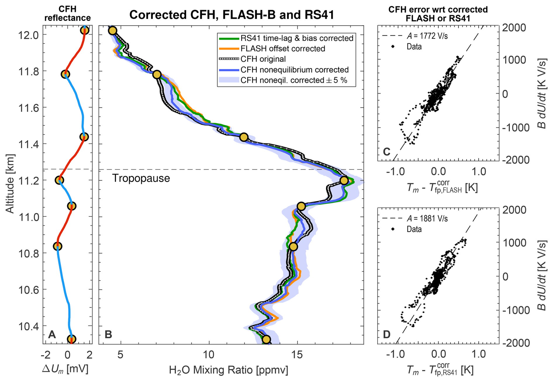
Figure 4 CFH-FLASH tandem sounding launched with a 2000 g rubber balloon on 13 March 2017 at 22:54 UT from Lindenberg Observatory (52.21° N, 14.12° E) together with a Vaisala RS41 radiosonde. (A) CFH mirror reflectance voltage U_m−2.5 V with Golden Points at the extremes (maxima and minima of U_m) separating sections of the balloon trajectory where the CFH mirror is too warm (red) or too cold (blue). (B) H₂O mixing ratio measured by CFH, FLASH and RS41. Orange curve: offset-corrected FLASH. Green curve: time-lag and bias corrected RS41. Black curve with gray data points: CFH original data. Blue curve: nonequilibrium corrected CFH. Light blue shading: ±5 % around nonequilibrium corrected CFH. (C) Scatter plot of the scaled time derivative of CFH mirror reflectance $B\cdot \mathrm{d}{U}_{\mathrm{m}}/\mathrm{d}t$ (see Eq. 8b) over the difference of the CFH mirror temperature and the offset-corrected FLASH frost point measurements yielding an effective sensitivity A = 1772 V s⁻¹. (D) Same as panel (C) but using the bias- and time-lag corrected RS41 frost point measurements yielding a very similar effective sensitivity A = 1881 V s⁻¹.

While the flight segment between 11.1 and 11.4 km could at first be confused with a time-lag error of CFH, the undershoots between 11.55 and 11.8 km and between 10.8 and 11.1 km show that the original CFH data suffer from controller/mirror oscillations, and not from a slow response of its mirror temperature signal. Conversely, the RS41 and FLASH-B hygrometers provide information about the actual humidity structure, but suffer from a dry bias in this flight section and have to be corrected first (Appendices B, C). Figure 4 also shows the profiles of the time-lag and bias-corrected RS41 (green curve) and the offset-corrected FLASH-B (orange curve). The discrepancies between these corrected profiles and the original CFH amount to ∼ 15 %, which is reduced to ∼ 5 % by the nonequilibrium correction of CFH (blue shaded area). This demonstrates the necessity and validity of the nonequilibrium correction of CFH for quantifying the frost point.

The two examples in this and the previous sections show that the use of mirror reflectance is a powerful diagnostic tool. Not only can the atmospheric frost point be determined at the Golden Points, but the time derivative of the reflectance also shows whether the mirror is too warm or too cold, allowing for appropriate correction. We therefore strongly recommend that chilled mirror instruments always provide the measured reflectance signal in addition to the mirror temperature.

5.3 Nonequilibrium correction versus treating CFH as time-lagged instrument

Chilled mirror hygrometers are actively controlled instruments and typically follow a second order response with multiple overshoots (e.g. Jacobs, 1993), i.e., the mirror temperature satisfies a second-order differential equation of the form ${\mathit{\tau }}^{\mathrm{2}}{d}^{\mathrm{2}}{T}_{\mathrm{m}}/\mathrm{d}{t}^{\mathrm{2}}+\mathrm{2}\mathit{\zeta }\mathit{\tau }\mathrm{d}{T}_{\mathrm{m}}/\mathrm{d}t+T_{\mathrm{m}}=f_{\mathrm{ext}}\left(t\right)$. Here, τ is the system's natural period of oscillation and ζ is its damping factor, which are defined, among other things, by the Joule heating of the mirror along with its thermal inertia, the PID settings, the H₂O gas phase kinetics, as part of the control system. Further, f_ext is the external forcing that results from the changing ambient humidity. Typically, the PID parameters are tuned such that the resulting system follows a damped oscillator response. This 2nd order differential equation with oscillatory behavior and the nonequilibrium equation (Eq. 5) are coupled and must be satisfied simultaneously. As $\mathrm{d}{U}_{\mathrm{m}}/\mathrm{d}t$ satisfies the physical constraint given by Eq. (8b), this could be interpreted as 1^st order behavior (erroneously assuming the general relationship $\mathrm{d}{U}_{\mathrm{m}}/\mathrm{d}t\propto \mathrm{d}{T}_{\mathrm{m}}/\mathrm{d}t$), unless one recognizes that the mirror temperature is actually a more complex function of the reflectance signal, T_m=T_m(U_m), via the heating power applied by the controller (in response to ambient frost point changes).

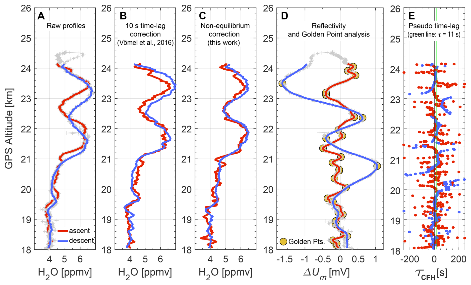
Figure 5 Water vapor mixing ratios during ascent and descent measured by CFH on 20 May 2014 22:51 UT over Lindenberg (serial 2L3407 with FW 6.40 on LI133). (A) Raw signal of H₂O mixing ratio ascent with smoothed mirror temperature (using a second-order, 15 s half-width, Savitzky-Golay filter) versus GPS altitude (air temperature and air pressure from iMet1-RSB radiosonde, serial 14246; telemetry software (Strato 9.54) applied an offset of 2.9 hPa to the pressure measurement). (B) Time-lag corrected mixing ratio profiles, using an e-folding time constant of 10 s, as in Vömel et al. (2016). (C) Nonequilibrium corrected mixing ratio profiles, using an effective sensitivity A = 800 V s⁻¹ for ascent and A = 2300 V s⁻¹ for descent. (D) Raw signal of mirror reflectance profiles (smoothed with a second-order, here in the stratosphere with a Savitzky-Golay filter with 21 s half width instead the standard 15 s) and associated Golden Points. (E) Ascent and descent profiles of the pseudo time lag constant τ_noneq, i.e. the mathematical time constant that would be required to reproduce the atmospheric frost point profile after applying the nonequilibrium correction. The median of all τ_noneq is 11 s (green line), i.e. close to the e-folding time constant of 10 s used for the time-lag treatment in panel (B).

Depending on the size of the damping factor ζ, the controller behavior can be overdamped (ζ > 1, sluggish approach to the instantaneous equilibrium without oscillations), critically damped (ζ = 1, faster approach to equilibrium without oscillations), underdamped (1 > ζ > 0, oscillatory approach to equilibrium with over- and undershoots), or unstable (0 > ζ, oscillations increase), assuming the forcing term to be constant. Figures 3 and 5 show that CFH often operates in the underdamped regime. Due to changes in the forcing term, it can happen that the mirror temperature oscillations are strongly underdamped for a few seconds and approach instability. Conversely, there are situations where the mirror temperature oscillations are overdamped and very close to a first order response. Under these latter conditions, a simple correction can be used to describe CFH, mimicking a time-lag similar to the behavior of RS41, and an exponential approximation to equilibrium is assumed (as in Miloshevich et al., 2004). This approach has been applied in the past (e.g. Vömel et al., 2007b, 2016; Hasebe et al., 2013) to match the measurements of stratospheric humidity features observed during both balloon ascent and parachute descent.

We revisit a CFH flight from Lindenberg in May 2014, where humidity features measured in the stratosphere during ascent and descent have been approximately matched in altitude using a time constant of 10 s (Vömel et al., 2016). This assumes a first-order response for the mirror temperature, $T_{\mathrm{fp}}\left(t\right)=T_{\mathrm{m}}\left(t\right)+{\mathit{\tau }}_{\mathrm{CFH}}\mathrm{d}{T}_{\mathrm{m}}/\mathrm{d}t\left(t\right)$, where τ_CFH is the time constant for the apparent time-lag (here 10 s), or equivalently ${\mathit{\chi }}_{{\mathrm{H}}_{\mathrm{2}}\mathrm{O}}\left(t\right)={\mathit{\chi }}_{{\mathrm{H}}_{\mathrm{2}}\mathrm{O},\mathrm{m}}\left(t\right)+{\mathit{\tau }}_{\mathrm{CFH}}\mathrm{d}{\mathit{\chi }}_{{\mathrm{H}}_{\mathrm{2}}\mathrm{O},\mathrm{m}}/\mathrm{d}t\left(t\right)$ in terms of water vapor mixing ratio.

Figure 5 compares the raw data (Fig. 5A) with the time-lag correction τ_CFH = 10 s (Fig. 5B), and the nonequilibrium correction, Eq. (8a) (Fig. 5C), which is based on the Golden Points and nonequilibrium correction (Fig. 5D). We determine the CFH nonequilibrium self-correction by using the CFH descent data to establish the a-priori for the ascent data and vice versa. Figure 5 reveals that at altitudes where both the ascent and descent exhibit simultaneous Golden Points, also both frost points agree well, and without any lag. The nonequilibrium correction provides a better match of the ascent and descent features in stratospheric humidity than the time-lag correction. This is because the nonequilibrium correction makes use of the mirror reflectance measurement through Eq. (8a) and corrects the main reason for the ascent/descent features mismatch, namely the nonequilibrium oscillations of the mirror temperature caused by the CFH controller, better than a time-lag treatment would. We have excluded the first 400 m of descent, like in Vömel et al. (2016), as they may be affected by an unstable airflow and short-term contamination from the payload. We have derived the effective sensitivity for the ascent, A_ascent = 800 V s⁻¹ and for the descent, A_descent = 2300 V s⁻¹, by fitting for the best match between ascent and descent humidity features. Differences in sensitivity of this magnitude are to be expected due to the higher ventilation during descent (υ_descent ∼ 20 m s⁻¹ and υ_ascent ∼ 5 m s⁻¹ and $A\sim {\mathit{\upsilon }}^{\mathrm{1}/\mathrm{2}}$).

The nonequilibrium correction is valid everywhere, whereas applying a time-lag correction is valid only within flight sections where the nonequilibrium excursions can be approximated by a first order response, such as in subsections of the flight shown in Fig. 5. To illustrate that the nonequilibrium error is qualitatively different from a time-lag error, but may appear locally as a time-lag error, we rewrite the nonequilibrium correction (Eq. 8a) in the mathematical form of a first order response: $T_{\mathrm{fp}}\left(t\right)=T_{\mathrm{m}}\left(t\right)+{\mathit{\tau }}_{\mathrm{noneq}}\mathrm{d}{T}_{\mathrm{m}}/\mathrm{d}t$ with the nonequilibrium “pseudo time-constant” ${\mathit{\tau }}_{\mathrm{noneq}}=B\left(t\right)/A\cdot (-\mathrm{d}{U}_{\mathrm{m}}/\mathrm{d}{T}_{\mathrm{m}})$. The term $-\mathrm{d}{U}_{\mathrm{m}}/\mathrm{d}{T}_{\mathrm{m}}$ (in V K⁻¹) contains the reflectance measurement U_m.

Therefore, τ_noneq (in s) can take both positive and negative values (see Fig. 5E) and is highly variable over time, which is not a physically meaningful quantity. Only the median value of the pseudo-time constant τ_noneq of 11 s agrees well with the 10 s used by Vömel et al. (2016), but with a standard deviation of 37 s around the median.

For these reasons, it is generally not appropriate to treat the response of chilled mirror instruments in the same manner as the response of polymer thin film sensors (as in e.g. WMO, 2024, their Table 12.7), because high-quality chilled mirror hygrometers do not suffer from time-lag of their mirror temperature (the thermistor measuring the mirror condensate temperature has a characteristic time in the order of 0.12 s for CFH, see Sect. 4.1.3), but from nonequilibrium errors.

5.4 Nonequilibrium correction versus low-pass filtering

The AquaVIT-1 intercomparison of atmospheric water vapor measurement techniques considered CFH as one of the “core” instruments to construct a metrological reference (Fahey et al., 2014), and the SPARC water vapor assessment II (WAVAS), which investigated biases and drifts of water vapor satellite retrievals with respect to frost point hygrometers, accepted CFH as a reference instrument (Kiefer et al., 2023), as did the WMO 2022 Upper-Air Instrument Intercomparison Campaign (Dirksen et al., 2024). Due to the generally high quality, it is often not necessary to apply corrective measures for errors of the CFH. Yet, averaging over extended sections (> 125 m in the stratosphere) of the balloon ascent profile by applying a Gaussian filter is part of the standard procedure for CFH data processing. This is intended to quantify and reduce uncertainty, at the expense of reducing vertical resolution, as described by Eqs. (1)–(5) in Vömel et al. (2016).

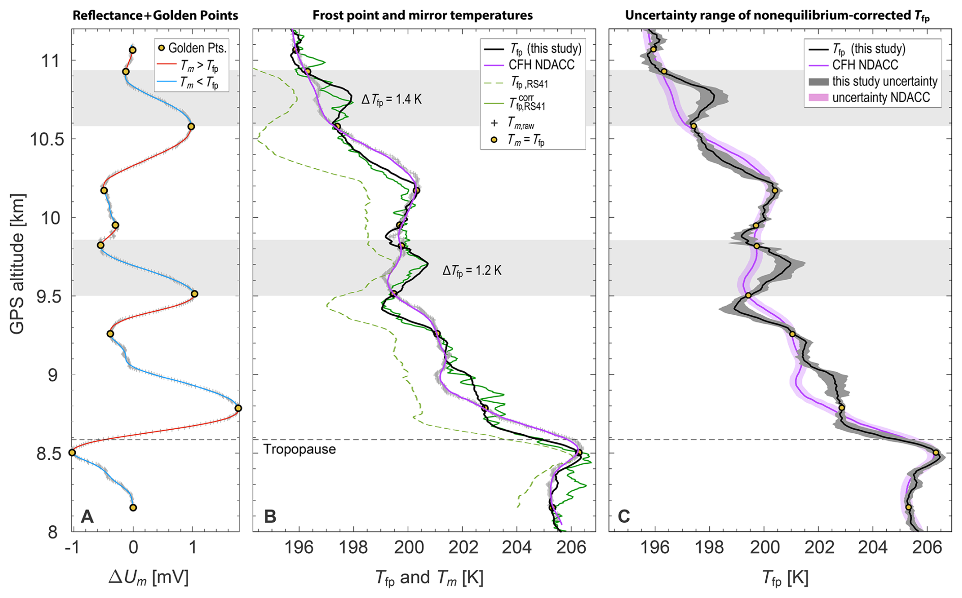
Figure 6 Frost point profiles in the lowermost stratosphere from the sounding in Ny-Ålesund on 21 February 2020 19:09 UT. (A) CFH mirror reflectance. Raw reflectance data (gray +), smoothed mirror reflectance colored red when mirror too warm and blue when mirror too cold, Golden Points (yellow circles). (B) Raw CFH mirror temperature (gray +), CFH Golden Points (yellow circles), RS41 frost point (Vaisala product, dashed green), RS41 time-lag and bias-corrected frost point for best fit at the CFH Golden Points (solid green), nonequilibrium corrected CFH mirror temperature using the mirror reflectance smoothed by a 15 s half-width Savitzky-Golay filter to calculate the effective sensitivity A from the corrected RS41 (solid black). The nonequilibrium corrected CFH profile (black solid line) fits to the stratospheric humidity features captured by the RS41 (green solid lines) much better than the NDACC Revision 0 (NDACC, 2020) profile (purple line). (C) Lines are the nonequilibrium-corrected CFH mirror temperature (black) and NDACC Revision 0 profile (purple) identical to panel (B). Dark gray shading: total uncertainty range of the CFH nonequilibrium correction (see Eq. 9). Purple shading: uncertainty range provided by NDACC (±2σ). The uncertainty ranges do not overlap in parts of the profile (e.g., gray-shaded sectors) with discrepancies up 0.8 K (15 % in H₂O mixing ratio).

Figure 6 compares the averaging by Gaussian filtering with the nonequilibrium correction using the example of a CFH-RS41 tandem flight on 21 February 2020 in Ny-Ålesund on Spitsbergen (Svalbard, Norway). The figure shows a nearly isothermal profile section (208–210 K air temperature) in the lowest stratosphere in polar winter. Since the relative humidity is sufficiently high (S_ice > 0.1), the RS41 radiosonde remains sensitive to moisture (e.g. Survo et al., 2015) and can be used as a reference for estimating the effective sensitivity parameter A in the stratosphere.

The effect of averaging and smoothing with the Gaussian filter can be seen by comparing the original CFH data (T_m,raw, gray crosses in Fig. 6B) and the pink “CFH NDACC” curve (with a vertical resolution provided in the NDACC data file ranging from 137 to 261 m for the flight section shown in Fig. 6). Gaussian filtering reduces here the noise in the mirror temperature, but does not correct the controller's nonequilibrium errors. The changes due to Gaussian filtering amount to ±0.2 K in the frost point temperature and about ±1 % in S_ice. In contrast, the nonequilibrium errors actually caused by controller oscillations are about a factor of 5 larger, as the comparison of the original CFH data (gray crosses) and the black curve “T_fp” shows. The nonequilibrium corrected CFH profile, T_fp, is closer to the moisture characteristics measured by the RS41 than to T_m,raw or to the Gaussian filtered curve. This example also shows that the actual atmospheric humidity profile between the Golden Points can be highly variable (e.g. the two moist features at altitudes highlighted by gray shadings in Fig. 6B). In this case, Gaussian filtering of the mirror temperature profile fails to capture the structure of the atmospheric humidity field seen by both RS41 and the nonequilibrium corrected CFH, and its uncertainties appear to be underestimated at certain altitudes (see Fig. 6C). Similarly, a first-order time lag treatment cannot capture the detailed structures of atmospheric moisture, the same is true for a mere interpolation of the Golden Points. Finally, 250 m boxcar averages (as used by NOAA) of the mirror temperature with a center of 9.75 and 10.75 km would also lead to a dry bias of about 1 K at the frost point, and the associated uncertainty, i.e., the standard error of the 250 m linear fit (Hall et al., 2016) would be underestimated.

Good control of the frost on the mirror is a tradeoff between producing many Golden Points ($\mathrm{d}U/\mathrm{d}t$ = 0) and minimizing the nonequilibrium error (small $|\mathrm{d}U/\mathrm{d}t|$). A strongly oscillating PID controller producing Golden Points at < 100 m vertical resolution, e.g. SKYDEW with its current PID implementation (Sugidachi et al., 2025), would be able to capture detailed humidity structures as in Fig. 6. However, PID controllers with strong oscillations tend to have a larger oscillation amplitude and thus a larger uncertainty (∼ 0.5 K) at the Golden Points (defined as the maximum mirror temperature difference ±1 s around Golden Points), as well as larger nonequilibrium errors. On the other hand, CFH has a well-tuned controller for background conditions of tropospheric and stratospheric humidity, with mostly small nonequilibrium errors. Nevertheless, rapid frost point changes can cause large nonequilibrium errors on CFH, with Golden Points more than 100 m apart. Thus, it is unclear whether PID control is the most appropriate approach to frost control of chilled mirror hygrometers. Control algorithms designed to “seek” Golden Points might be a valid alternative to PID control, but we restrain from discussing this further, as we are not aware of any implementation of this type yet. In any case, no matter the control approach, control-induced oscillations can be corrected with Eq. (5).

5.5 Uncertainty of the nonequilibrium correction

In this section, we describe two metrics to quantify the uncertainty of the nonequilibrium correction procedure described in Sect. 4.2. The first metric quantifies uncertainty by comparing the final (i.e., nonequilibrium corrected) CFH frost point estimate to the a-priori reference estimate. The second metric quantifies the uncertainty of the nonequilibrium correction method itself.

For the first metric, we quantify the uncertainty as the root mean square error (RMSE) between the a-priori reference profile (e.g., RS41 corrected for residual time-lag and bias errors using the CFH Golden Points), and the a-posteriori atmospheric frost point profile, i.e., CFH corrected for nonequilibrium errors. We term this uncertainty (at 2σ) u_REF, with u_REF = 2 × RMSE (e.g., in Fig. 6B, u_REF = 2 × 0.36 K = 0.72 K). From the 70 CFH-RS41 tandem flights analysis in Sect. 6, we find a root mean square error < 0.16 K between the CFH corrected and RS41 corrected profiles at 125 m vertical resolution. Together with the mirror temperature uncertainty $u_{T_{\mathrm{m}}}$ = 0.11 K (at 2σ) for ice films (Sect. 2.5), this gives an overall uncertainty < 0.4 K (at 2σ) for the nonequilibrium corrected frost point profiles (when using, prior to correction, a 15 s half-width second-order Savitzky-Golay filter for sampling the Golden Points and calculating the derivative of the mirror reflectance signal, and a 25 s full-width boxcar filter for smoothing the raw relative humidity signals). An uncertainty in frost point < 0.4 K at 125 m vertical resolution reduces to < 0.2 K at 500 m vertical resolution (as 500 m = 4 × 125 m, i.e. the uncertainty is reduced by a factor 4${}^{\mathrm{1}/\mathrm{2}}$). Together with an uncertainty of 0.3 hPa in RS41 pressure from GPS (Vaisala, 2018b), this translates to less than 4 % uncertainty in water vapor mixing ratio (see also Hall et al., 2016).

For the second metric, we quantify the uncertainty of the nonequilibrium correction ($B/A\times \mathrm{d}{U}_{\mathrm{m}}/\mathrm{d}t$) using a sensitivity analysis, where we vary the half-width of the Savitzky-Golay filter (used to smooth the reflectance signal) by a factor 0.5, 1 and 2 (i.e., 7, 15, 30 s), while keeping all other parameters constant. For each filter width, we sample the CFH Golden Points, find best fits for the RS41 time-lag and bias correction parameters, calculate the effective sensitivity parameter A, and finally calculate the nonequilibrium corrected CFH profile. We estimate the (2σ) uncertainty of the nonequilibrium correction as the maximal deviation in the final correct CFH profiles between all Savitzky-Golay filter widths: $u_{\mathrm{SG}}=max\left(T_{\mathrm{fp},\mathrm{corr}\{\mathrm{7}\mathrm{s},\mathrm{15}\mathrm{s},\mathrm{30}\mathrm{s}\}}\right)-min\left(T_{\mathrm{fp},\mathrm{corr}\{\mathrm{7}\mathrm{s},\mathrm{15}\mathrm{s},\mathrm{30}\mathrm{s}\}}\right)$. Adding in quadrature the mirror temperature uncertainty (2σ) $u_{T_{\mathrm{m}}}$ and the statistical uncertainty (2σ) u_m of the 25 s average (calculated as in Dirksen et al., 2014, their Eq. A2, then multiplied by 2), we calculate the total uncertainty u (2σ) of the nonequilibrium corrected frost point as:

$$\begin{array}{}\text{(9)}& u=\sqrt{u_{\mathrm{SG}}^{\mathrm{2}}+u_{T_{\mathrm{m}}}^{\mathrm{2}}+u_{\mathrm{m}}^{\mathrm{2}}}.\end{array}$$

The total uncertainty u is depicted as gray shaded area (±u) in Fig. 6C. The mean value for the total uncertainty for the flight section (8–10.2 km) is 0.32 K, while the standard deviation of non-equilibrium corrected CFH data (black lines in Fig. 6) with respect to time-lag and bias corrected RS41 data is 0.36 K.

The second metric u can be used to validate the first metric. The nonequilibrium corrected CFH data may be considered valid only in-flight segments where $|T_{\mathrm{fp},\mathrm{RS}\mathrm{41}}^{\mathrm{corr}}-T_{\mathrm{fp},\mathrm{CFH}}^{\mathrm{corr}}|<u$. This is the best ad-hoc method to validate the uncertainty of our retrieval in the absence of an SI-traceable sensor of similar or better accuracy as CFH. It also allows detection of measurement artifacts, such as contamination from the wake of the balloon or strong anomalies in airflow through the tube. We note that this (rather conservative) validation technique has not been applied to this work.

Filtering widths from ±7 to ±30 s give a reasonable range of structure-preserving smoothing filters for the mirror reflectance. Excessive smoothing (e.g., by ±300 s) would strongly smooth out features from the reflectance data, resulting in erroneous $\mathrm{d}{U}_{\mathrm{m}}/\mathrm{d}t$ estimates and “fantasy” Golden Points (see Fig. D2). As a consequence, the fitted time-lag and bias corrected RS41 as well as the fitted effective sensitivity parameter A would not be meaningful. No smoothing would retain all noise from the reflectance data, which may lead to erroneous $\mathrm{d}{U}_{\mathrm{m}}/\mathrm{d}t$ estimates as well as a large amount of incorrectly sampled Golden Points due to noise. Moreover, no smoothing or undersmoothing might pick-up high frequency oscillations with full anti-correlation of T_m and U_m. Some CFH flights show an eigenfrequency of 5 s (see Fig. D1), which are not of atmospheric origin and would thus produce an incorrect correction.

For the Golden Points, we calculate uncertainty (2σ) as:

$$\begin{array}{}\text{(10)}& u_{\mathrm{GP}}=\sqrt{u_{\mathrm{timing}}^{\mathrm{2}}+u_{T_{\mathrm{m}}}^{\mathrm{2}}},\end{array}$$

where u_timing is the ±1 s timing uncertainty in sampling the Golden Points, using the same uncertainty metric as Sugidachi et al. (2025, their Eq. 14, then multiplying by 2). From our analysis of 70 flights presented in Sect. 6, we find, at 2σ, u_timing = 0.12 K for the liquid condensate, 0.16 K for the first ice condensate and 0.15 K for the second ice condensate. This translates, using Eq. (10), to a total (2σ) uncertainty u_GP of the Golden Points of 0.23 K for the liquid film and 0.19 K for the ice films, i.e. < 0.3 K at the dew point and < 0.2 K at the frost point. Figures 2 and 7 showcase that the vast majority of CFH Golden Points remain within these uncertainty limits if shifted by ±1 s. This is because $|\mathrm{d}{T}_{\mathrm{m}}/\mathrm{d}t|$ is generally well-constrained by CFH's PID controller, and heat equilibrates rapidly (∼ 120 ms) across the mirror disk (Sect. 4.1.3).

5.6 Flight-to-flight variability

A well-adjusted CFH is one for which the combined effect of all sources of uncertainty in frost point (or dew point) measurements is better than 0.2 K, and systematic errors, which most likely affect long-term climate series, are demonstrably smaller than 0.1 K (Vömel et al., 2016). In fact, the nonequilibrium analysis of the present work confirms this performance for a majority of the analyzed CFH data points (for statistics see Sect. 6.2).

As mentioned earlier, not all instruments or flight legs are equally affected by nonequilibrium errors. As shown by Eq. (5) ($\mathrm{1}/A^{\prime }\cdot \mathrm{d}U/\mathrm{d}t\sim {\mathit{\chi }}_{{\mathrm{H}}_{\mathrm{2}}\mathrm{O}}\left(T_{\mathrm{m}}\right)-{\mathit{\chi }}_{{\mathrm{H}}_{\mathrm{2}}\mathrm{O}}\left(T_{\mathrm{fp}}\right)$), the reasons for this are the quality of the ice film, which is determined by the properties and cleanliness of the mirror, by the condensate thickness at the PID setpoint and by the cleaning cycles (all described by A^′), as well as the properties of the vertical H₂O profile (${\mathit{\chi }}_{{\mathrm{H}}_{\mathrm{2}}\mathrm{O}}$), which determines the history in the integral part of the PID with a fixed setpoint (at low H₂O mixing ratios, a minute change in reflectance corresponds to larger deviations from frost point than at high H₂O mixing ratios). Subsequently, we discuss a few selected cases with widely varying performance and in Sect. 6 we discuss the statistics of the 70 analyzed soundings.

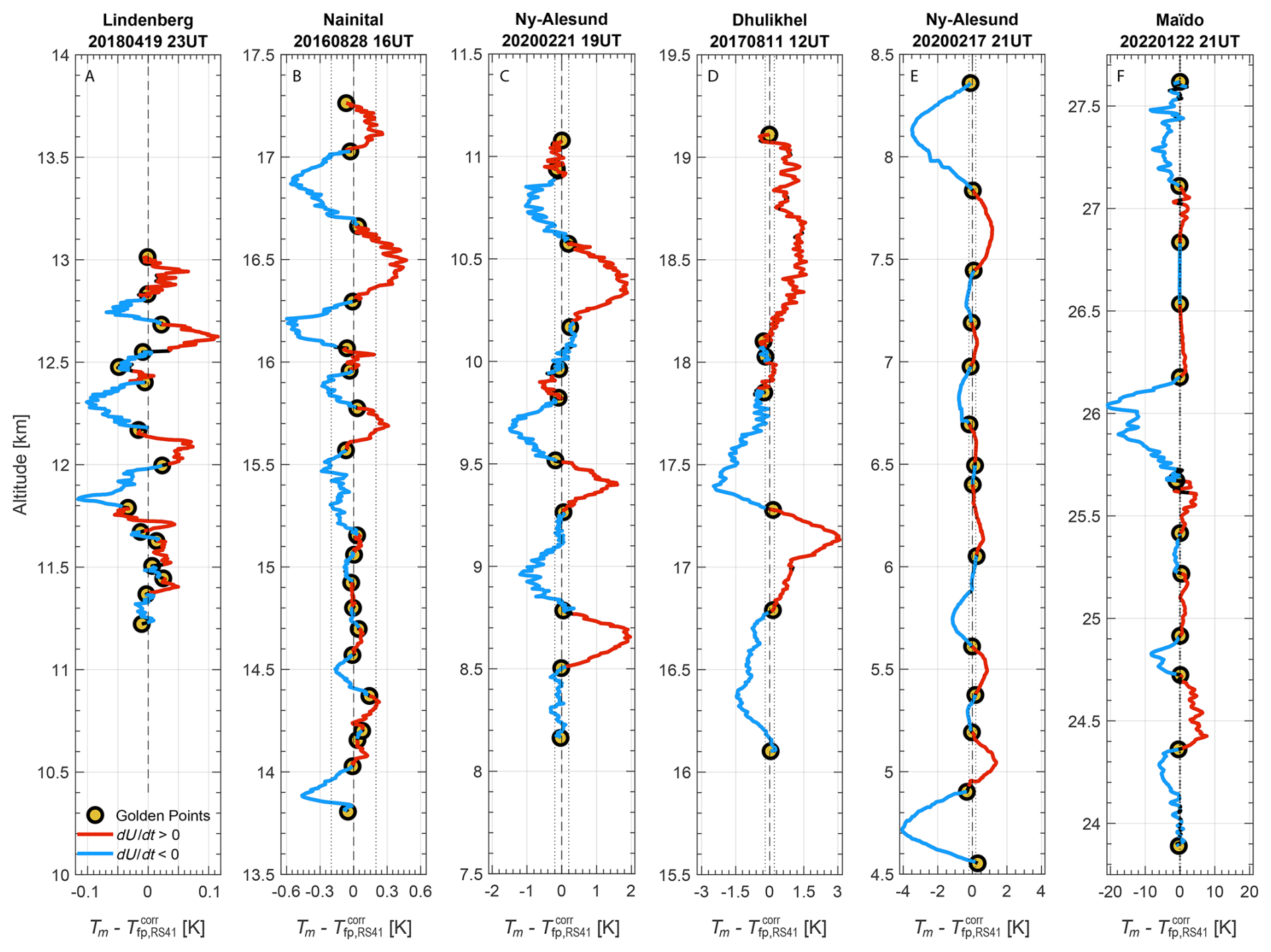
Figure 7 Four-kilometer slabs of various soundings with CFH, sorted according to nonequilibrium error. Slabs start after the second cycle (at T_fp = −53 °C) and end at the hygropause. We use the higher reliability of RS41 below the hygropause to correct CFH in panels (A)–(E). An exception is panel (F), which shows the CFH measurement in the core of the Hunga Tonga-Hunga Ha'apai plume, for which CFH was corrected assuming a background mixing ratio of 5 ppmv. Panels (A) and (F) will be discussed in detail in the following subsections.

Figure 7 shows a collection of nonequilibrium errors obtained from six flights. The magnitude of the error in frost point temperature increases from left to right and varies between less than 0.1 K to several K, and from being symmetric to highly asymmetric in terms of frost point. Three of these six examples are subsequently discussed in more detail (Sect. 5.6.1 and 5.6.2).

5.6.1 Case Study: Stratospheric streamer with enhanced H₂O over Lindenberg

Figure 7A shows the CFH measurements at Lindenberg (52.21° N, 14.12° E) on 19 April 2018 below the hygropause. About 10 km higher, in the stratosphere, the same sounding showed a significant increase in the H₂O mixing ratio of 1.5 ppmv above the background value of 4.8 ppmv at an altitude of 22.0–22.5 km. This anomaly is unusual and the question arises as to whether this is a false measurement. In order to directly compare the measurements during the ascent and descent, we show the H₂O profile as a function of potential temperature in Fig. 8. In fact, the anomaly can also be found in the descent data between 535 and 550 K. The CFH nonequilibrium correction corroborates the very good altitude agreement during ascent and descent.

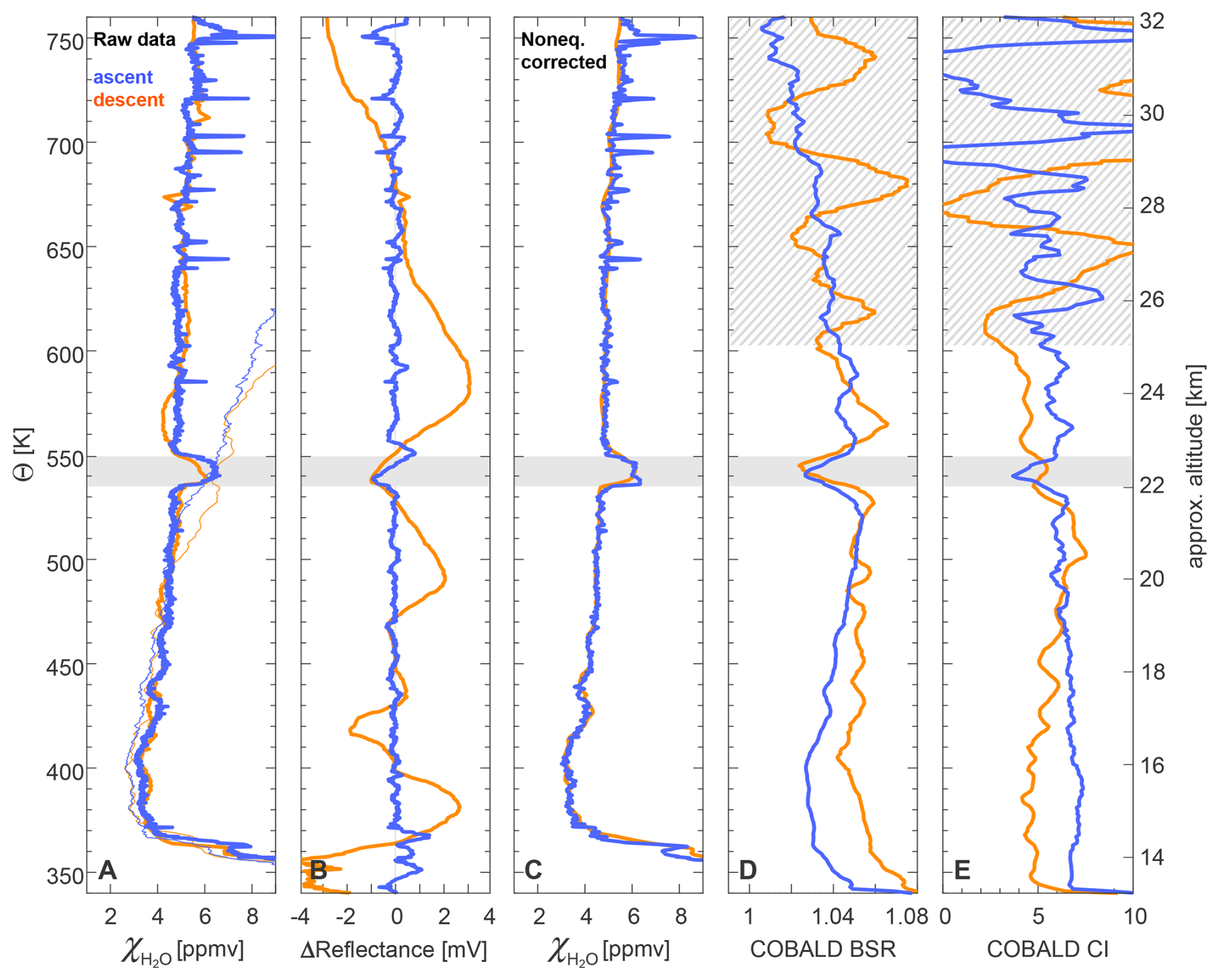
Figure 8 Balloon sounding on 19 April 2018 in Lindenberg (52.21° N, 14.12° E) showing remarkable H₂O and particle backscatter anomalies (gray shading) in measurements by CFH and the backscatter sonde COBALD during ascent (blue lines) and descent (orange lines). (A) H₂O mixing ratios retrieved from CFH raw data. Thin lines show the RS41 data (Vaisala product). In this sounding, RS41 lost sensitivity above potential temperature level 500 K (≈ 20.5 km altitude). (B) CFH reflectance signal. (C) Nonequilibrium correction of the CFH mixing ratio, making the blue ascent and the orange descent lines almost coincide. (D) COBALD backscatter ratio (BSR_455 nm) at 455 nm, with 10 K (potential temperature) moving average. (E) COBALD Color Index CI = (BSR_940 nm − 1) $/$ (BSR_455 nm − 1), also with 10 K moving average. Hatched area: above 600 K the backscatter signal is too noisy during descent, possibly due to excessive swinging of the dangling payload.

For the nonequilibrium correction of the ascent, we use the morphological sensitivity A^′ determined for the upper troposphere in Fig. 7A. The validity of this procedure is not self-evident, as the morphology of the ice film may have changed during the 10 km interval of ascent. However, the RS41 provides no information above 20 km, so assuming the same morphology is the most useful assumption. We also use a constant morphological sensitivity A^′ for the descent, but the much higher ventilation due to the fast descent has to be taken into account. We take account of the about five times faster descent rate resulting in enhanced ventilation of the mirror by virtue of $\mathrm{\Delta }{x}_{\mathrm{diff}}\propto {\mathit{Re}}^{-\mathrm{1}/\mathrm{2}}\propto {\mathit{\upsilon }}_{\mathrm{flow}}^{-\mathrm{1}/\mathrm{2}}$, which reduces the Prandtl layer thickness Δx_diff and enhances the effective sensitivity A by 5${}^{\mathrm{1}/\mathrm{2}}$ relative to the ascent of the balloon. The excellent agreement between the humidity measured during ascent and descent strengthens the validity of these assumptions.

The aerosol backscatter probe COBALD (Brabec et al., 2012) and an electrochemical ozone probe (ECC) flew on the same payload. The ECC provides some evidence of this anomaly with a local decrease in ozone concentration around 540 K, but unfortunately suffered from technical problems and will therefore not be discussed further. The COBALD data show a minimum in the backscattering (both in the 940 and 455 nm channels) in the same layer as the H₂O anomaly (Fig. 8D). CFH and COBALD measurements consistently show that the air mass at 540 K has a different origin than the rest of the profile. High humidity and low number density of aerosol particles point to the polar vortex as a possible region of origin. The air from there is “old”, meaning that methane oxidation is advanced, which increases the H₂O mixing ratio, and the particle number density is low because large particles have precipitated on the transport route to the poles. This is confirmed by the COBALD color index, which shows a minimum of about 4–5 in this layer. This fits a lognormal distribution of aerosol particles with a width σ = 1.6 and a mode radius of 40–50 nm, whereas the typical mid-latitudinal mode radius of 60–80 nm yields a color index of about 6–7. Finally, the RS41 was not able to detect the stratospheric H₂O anomaly, not even qualitatively, as it already lost sensitivity to humidity at lower altitudes (i.e. the humidity signal cannot be distinguished from the noise in the capacitance measurement).

So, the CFH/COBALD tandem with nonequilibrium CFH correction reveals that locally elevated H₂O over Lindenberg at about 540 K (22.5 km) together with a significant change in the aerosol properties is not an artifact. Rather, it is a true atmospheric signal most likely caused by an erosion of the polar vortex in spring 2018 creating a thin layer with high water vapor and low aerosol and ozone concentrations.

5.6.2 Case Study: Hunga Tonga-Hunga Ha'apai stratospheric plume

Figure 9A shows the CFH measurements from Maido Station on Reunion Island (21° S, 55° E) on the evening of 22 January 2022. The massive explosive eruption of the submarine volcano Hunga Tonga-Hunga Ha'apai (HTHH) (21° S, 175° W) injected 50–150 Tg H₂O (e.g. Vömel et al, 2022; Khaykin et al., 2022; Millán et al., 2022) and about 0.4 Tg SO₂ into the stratosphere (Millán et al., 2022). The Tonga volcano Rapid Response Experiment (TR²Ex) at the Maïdo observatory enabled in-situ balloon-borne measurements in the core of the main volcanic plume as it moved over Réunion Island 6 to 8 d after the eruption.

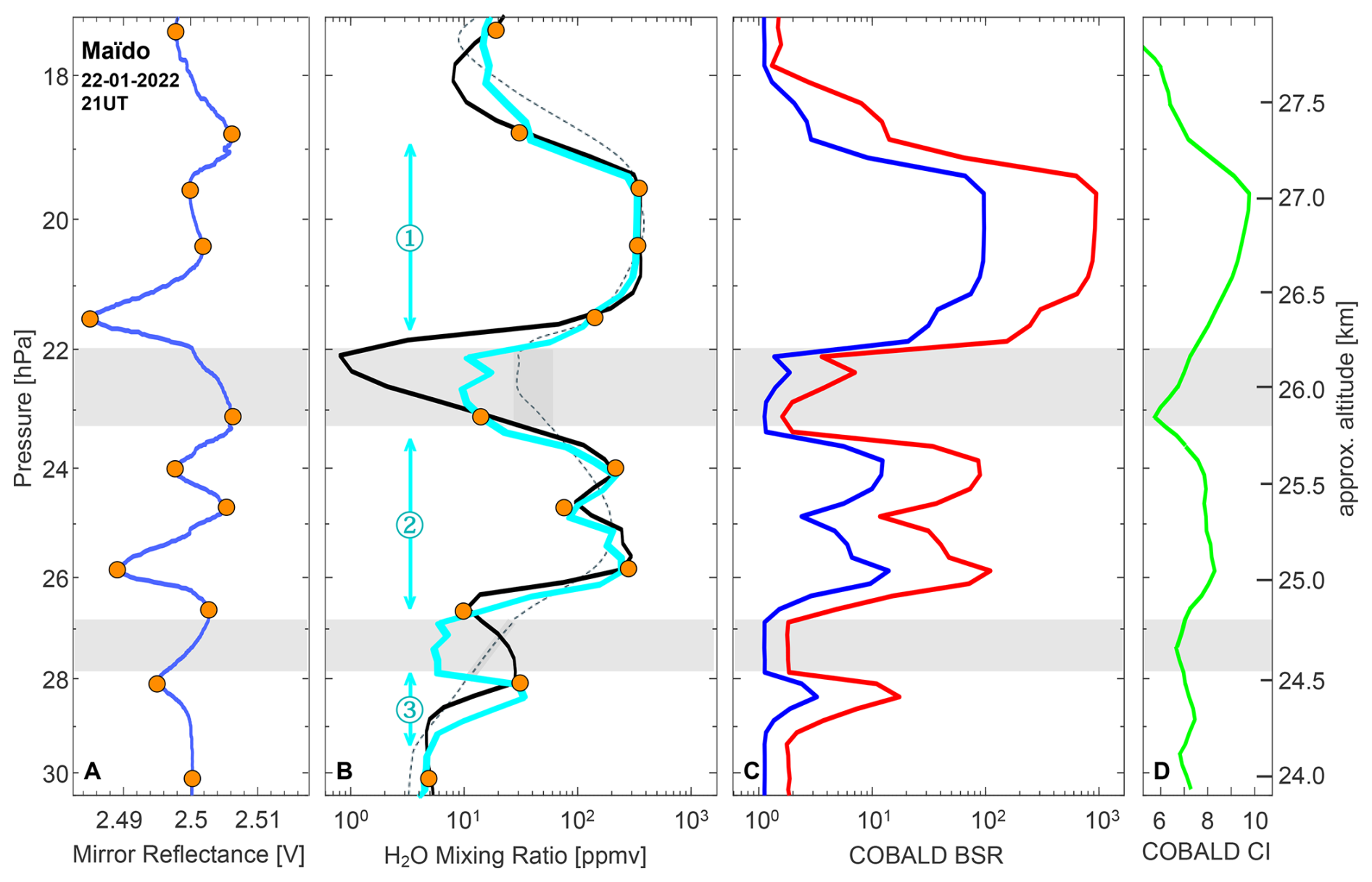
Figure 9 CFH-COBALD tandem measurements launched from the Maïdo Observatory in Réunion Island (21° S, 55° E) ascending into the main plume of the volcanic eruption of the Hunga Tonga–Hunga Ha'apai (HTHH) submarine volcano on 22 January 2022 at 21:00 UT. (A) CFH reflectance signal (blue line) and Golden Points (orange circles). (B) CFH raw data of H₂O mixing ratio (black line); nonequilibrium-corrected CFH mixing ratio (cyan); CFH data with 250 m smoothing (thin dotted line) as used by Evan et al. (2023). (C) Aerosol backscatter ratio measured by COBALD at 940 nm (BSR_940 nm, red line) and 455 nm (BSR_455 nm, blue line). (D) Aerosol Color Index measured by COBALD, CI = (BSR_940 nm − 1) $/$ (BSR_455 nm − 1). Gray shaded areas mark the largest errors in the H₂O profile that occur in the H₂O minima (i.e. in regions of the atmosphere unperturbed by the volcanic plume). H₂O mixing ratios (this work), backscatter ratios and color index in panels (B), (C), and (D) are displayed with 0.25 hPa (i.e., 50–100 m) binning.

The H₂O profile shown by Evan et al. (2023) is the thin dotted line in Fig. 9B; it has only a coarse vertical resolution (see polygonal line with 250 m linear elements in Fig. 3 of Evan et al., 2023) and exhibits only the two H₂O maxima. The original data show much more structure, but also a minimum that extends to an unrealistic 1 ppmv (bold black line in Fig. 9B). The correlation with the aerosol measurements (Fig. 9C) has a linear correlation coefficient R² = 0.61 (in log BSR_940 nm over $\log {\mathit{\chi }}_{{\mathrm{H}}_{\mathrm{2}}\mathrm{O}}$). Applying the CFH nonequilibrium correction to the data with high vertical resolution increases the level of correlation between the aerosol and H₂O profiles to R² = 0.86. We assumed a reference water vapor mixing ratio value of 5.5 ppmv at 27.5 hPa as a-priori for the nonequilibrium correction, in line with a background value for the COBALD aerosol measurement at that altitude and with Aura/MLS background H₂O profiles the days before. Due to the large deviations in frost point, the nonequilibrium correction was performed in partial pressure instead of frost point (i.e. Eq. 5 instead of Eq. 6). No RS41 or FLASH was present on that flight. In view of the large nonequilibrium errors, the uncertainty in the reference water vapor mixing value (< 10 %) is not of great importance compared to the benefits of applying the nonequilibrium correction.

The nonequilibrium correction allows us to compute the RH profile and compare it with the backscatter ratio (BSR, Fig. 9C) and color index (CI, Fig. 9D) of the COBALD sonde, both in high resolution. It is interesting to compare the three layers with increased H₂O mixing ratio between 19–22 hPa (layer 1), 24–26 hPa (layer 2) and 28–29 hPa (layer 3). In layer 1, there is a clear increase in the color index to values of CI = 8.5–10, which indicates effective particle radii of 0.35–0.5 µm (assuming H₂SO₄–H₂O droplets at RH_ice = 40 % and lognormal width σ = 1.6). In layer 2, the color index is slightly lower, with values around 8, in line with effective particle radii of about 0.3 µm. In layer 3, there is no clear correlation between H₂O mixing ratio and color index, but CI ∼ 7 suggests effective particle radii of about 0.15 µm (similar to unperturbed regions with CI ∼ 6, σ = 1.8 and RH_ice = 1 %). While the backscatter ratio is influenced by mixing with unperturbed air during an atmospheric transport time of about one week since the eruption occurred, the color index is virtually unaffected by mixing. Therefore, the difference between the color indices of the three layers suggests that much more H₂SO₄ conversion occurred in layer 1 than in layer 3. The H₂SO₄ then condenses onto existing particles or forms new particles that coagulate with existing ones, both of which contribute to particle growth. The likely reason for the faster conversion of SO₂ to H₂SO₄ is the higher humidity in layer 1, which exceeds that in layer 3 by about an order of magnitude. The combination of the high-resolution CFH and COBALD measurements in Fig. 9 and their interpretation is fully consistent with and supports the work of Asher et al. (2023).

Since the CFH reflectance measurement and COBALD's backscatter measurement arise from completely different measurement principles, the strong correlation is an impressive indicator for the validity of the nonequilibrium correction. The gray shaded areas indicate the largest errors in the H₂O profile, which occur in the H₂O minima. The resulting errors of up to 20 K in the frost point and more than a factor of 10 in the H₂O mixing ratio between the H₂O-enriched layers 1 and 2 are in flagrant violation of the target set by the WMO. However, it must also be clear that ignoring the unperturbed regions outside of the H₂O-enriched layers, as done by Vömel et al. (2022) and Evan et al. (2023), has little influence on the overall assessment of this extraordinary eruption.

5.7 Nonequilibrium self-correction

As mentioned in Sect. 4.3, a dense array of Golden Points along the vertical profile of a balloon ascent can enable a self-correction of a chilled mirror instrument. Self-correction accomplishes independence of other instruments that have higher vertical resolution (at lower accuracy), such as FLASH-B or RS41. Recently, there has been a development in this direction in the form of the Peltier-based chilled mirror hygrometer SKYDEW (Sugidachi et al., 2025). While the Golden Points of CFH are typically separated by a few hundred meters (see multiple examples in Figs. 2–9), SKYDEW's Golden Points are typically 15 m apart in the troposphere and 20–25 m in the stratosphere. Figure 10 illustrates this feature of SKYDEW that has the potential to lead to a better constraint of the frost point. However, Fig. 10B also shows that the very large amplitude of the nonequilibrium excursions leads to strong temporal changes, $\mathrm{d}{T}_{\mathrm{m}}/\mathrm{d}t$, at the Golden Points. This renders the retrieval of precise timings of the Golden Points along the balloon trajectory difficult. Even sampling time differences between T_m and U_m of less than 1 s can cause SKYDEW to suffer large uncertainties in the Golden Point timing, leading to incorrect Golden Points temperatures. This demonstrates that the perceived advantage of a denser Golden Point array, in terms of vertical resolution, can easily become a disadvantage in terms of frost point accuracy at the Golden Point on instruments with large nonequilibrium excursions.

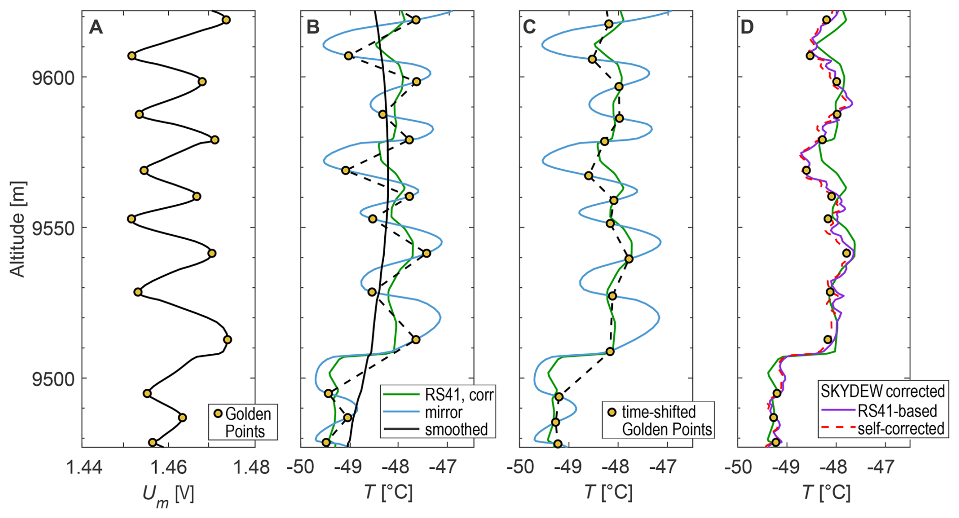
Figure 10 Self-correction procedure of SKYDEW (serial 20570, firmware 1.0), launched in tandem with a Vaisala RS41-SGP (V1021230) from the Lindenberg Observatory on 18 July 2023 at 21:06 UT. (A) SKYDEW mirror signal (upscaled from 1 to 5 Hz with linear interpolation to allow sub-second synchronization of U_m and T_m, then smoothed with a gaussian filter with an equivalent sample size of about 2 s in order to retain high temporal resolution) and the detected Golden Points (minima/maxima). SKYDEW uses light scattering instead of reflectance as its feedback signal, such that, in contrast to CFH, the mirror signal increases as the mirror condensate is growing and vice versa. (B) SKYDEW mirror temperature (blue) with Golden Points marked in yellow. The linear interpolation between Golden Points is shown as a black dashed line. The Golden Points “zig-zagging” effect is not an atmospheric effect and is due to a misalignment of 0.4 s between the mirror temperature and mirror signal values provided in the telemetry frame. The black line is a gaussian smoothing of the Golden Points linear interpolation (with an equivalent sample size of about 25 s or 125 m), similarly to Sugidachi et al. (2025) for the upper troposphere. (C) Effect of correcting for a 0.4 s delay in the mirror temperature telemetry signal on the position of Golden Points and linear interpolation thereof (D). SKYDEW nonequilibrium corrected mirror temperature, using RS41 time-lag and bias-corrected, and SKYDEW smoothed (B) as a-priori reference to determine A.

In Fig. 10C, we have shifted the mirror temperature data by 0.4 s (about 2 m vertical distance) relative to the reflectance signal, which can remove most of the atmospherically meaningless oscillation of the Golden Points for this particular case (i.e., T_m is shifted such that the RMS difference between the maxima-only and minima-only polygonal lines is minimized). After this synchronization of U_m and T_m, the Golden Points of SKYDEW can be used without further nonequilibrium correction, albeit with a vertical resolution of 15–25 m and a sampling uncertainty of ±1 s in the Golden Points (Sugidachi et al., 2025) associated with a steep slope $\mathrm{d}{T}_{\mathrm{m}}/\mathrm{d}t$. For finer structures to be resolved, SKYDEW requires a nonequilibrium correction, e.g. by means of a time-lag and bias-corrected RS41 in the same way as done for CFH (violet solid line in Fig. 10D).

Alternatively, SKYDEW can be self-corrected: by using the polygonal line defined by the neighboring Golden Points as a-priori reference in the nonequilibrium correction procedure, we can determine the sensitivity A and obtain the dashed red line in Fig. 10D. The good agreement (< 0.15 K) with the nonequilibrium corrected profile based on RS41 demonstrates the high potential of this procedure, which allows SKYDEW to be nonequilibrium corrected without a second independent sensor. However, in the absence of an additional sensor suited for the stratosphere, it remains unclear if the self-correction procedure presented here would work at 10 km higher altitudes. Also, due to the steep slopes $\mathrm{d}{T}_{\mathrm{m}}/\mathrm{d}t$ at the Golden Points, even with synchronized U_m and T_m, the noise in the measurements leaves SKYDEW's Golden Points with finite errors that can be quantified from Fig. 10C with ±1 s Golden Point timing uncertainties to be about ±1 K in this case (see Sect. 5.5). This calls for a better feedback control to reduce the amplitude of the nonequilibrium excursions, or for sub-second telemetry.

6 CFH nonequilibrium error statistics

In order to statistically evaluate the nonequilibrium error of CFH, we have analyzed a total of 70 RS41-CFH nighttime tandem soundings according to the procedure described in Sect. 4.2. A complete list of these 70 soundings is provided in Appendix A. Of these, 26 were performed during the StratoClim 2016-2017 campaigns in India and Nepal (Brunamonti et al., 2018), 40 during routine soundings in Lindenberg flown together with a COBALD backscatter sonde (Brabec et al., 2012; Vömel et al., 2016) between March 2016 and May 2019, and 4 during development and test flights for other instruments in Ny-Ålesund in February 2020 (Jorge et al., 2020). Except for one flight in Lindenberg, the CFH PID controller version is “6.44”, which is the standard version. Before data analysis, we eliminated flight segments that were rejected based on an NDACC quality check Revision 0 (i.e., flagged as “not valid”), e.g. due to mirror cleaning cycles, contamination or temperature/reflectance artifacts (NDACC, 2020; see also Vömel et al. (2016)). Furthermore, we restricted the analysis to night time measurements, since CFH daytime profiles tend to suffer from incomplete solar filtering and are more susceptible to noise (Hall et al., 2016) in the reflectance signal that would affect the quality of the reflectance-based statistical analysis.

Based on these 70 soundings, we show in Sect. 6.1 that there is a large film-to-film variability of the effective sensitivity parameter A, which makes a separate treatment of each sounding inevitable. Section 6.2 shows that the deviations between the reported mirror temperature and the nonequilibrium-corrected frost point are typically better than 0.5 K (corresponding to uncertainties < 9 % in the H₂O mixing ratio in the lower stratosphere). Greater deviations can occur when the morphology of the ice on the mirror is poor (e.g., coarse ice crystals), resulting in low A^′ (Eq. 2) and/or if the H₂O mixing ratio in the atmosphere changes significantly. In these cases, the nonequilibrium correction can remove 80 %–90 % of the nonequilibrium error. This, in turn, allows a reduction in the uncertainty (at a given vertical resolution) of the frost point estimates that occur under nonequilibrium conditions, and helps discern true atmospheric features from measurements artifacts.

6.1 Large film-to-film variability of the effective sensitivity parameter A

Figure 11 shows the effective sensitivity parameter A derived for the three condensate layer types (liquid film, first and second ice film) for each of the 70 flights. The values span about two orders of magnitude and vary from film-to-film and from flight-to-flight. This large variability does not allow the use of a fixed value of A for all flights, not even for instruments that have been recovered and flown again, using the identical mirror and optical hardware. This complicates the design of feedback controllers of consistently good performance, i.e. with the same sufficiently large A. Most likely, the variability is due to different film morphologies, themselves associated with the mirror surface properties (impurities, coatings, etc.), prevailing temperatures, ventilation, ambient H₂O molecule number density, cooling rate, supersaturation and possibly coalescence/sintering experienced during film formation. Variability in balloon ascent rate might play a minor role as well, as the boundary layer thickness of the airflow over the mirror is part of the effective sensitivity and depends on the flow conditions inside the inlet tubes. Over 95 % of the derived effective sensitivity values are larger than 1000 V s⁻¹ in the CFH data set we analyzed, which generally results in small mirror temperature deviations from equilibrium, as ($p_{\mathrm{vap}}\left(T_{\mathrm{m}}\right)-p_{\mathrm{vap}}\left(T_{\mathrm{fp}}\right)\propto \mathrm{1}/A\mathrm{d}{U}_{\mathrm{m}}/\mathrm{d}t$).

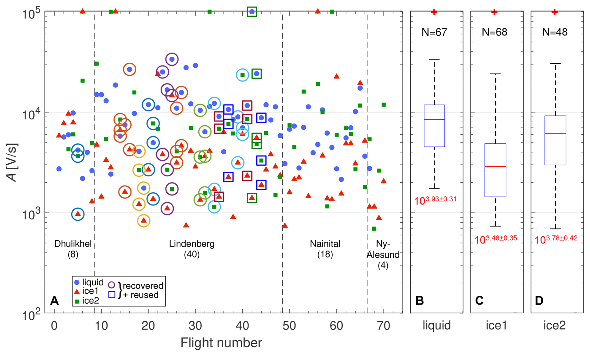
Figure 11 Sensitivities (in V s⁻¹) derived from 70 CFH-RS41 tandem soundings. (A) Sensitivity A of each individual soundings for the liquid film (blue), first ice film (red) and second ice film (green). Soundings with recovered and reused instruments are shown with frames. The sensitivities span about 2 orders of magnitude and vary from film-to-film and from flight-to-flight. (B–D) Distribution of the sensitivities shown as boxplots in log-scale for each of the three condensate layers. The box shows the median (horizontal red line, second quartile q₂), the 25 % (q₁) and the 75 % (q₃) percentiles, i.e. 50 % of all data are in the interquartile range q₃−q₁ (blue box). The whiskers show the mild outliers of A in logarithmic scale between 1 % and 99 % (or, more accurately, between $q_{\mathrm{1}}-\mathrm{1.5}\times (q_{\mathrm{3}}-q_{\mathrm{1}})$ and $q_{\mathrm{3}}+\mathrm{1.5}\times (q_{\mathrm{3}}-q_{\mathrm{1}})$). Numbers in red display are the median +/- the robust standard deviation (defined as half the difference between the 84.13 % and the 15.87 % percentiles). The first ice film has the lowest median effective sensitivity (∼ 2884 V s⁻¹), the liquid film the highest median effective sensitivity (∼ 8511 V s⁻¹), and the second ice film an intermediate ∼ 6026 V s⁻¹.

The first ice-film (triggered by the cleaning cycle at −15 °C mirror temperature) has the smallest effective sensitivity, likely due to an ice film with fewer and larger ice crystals, which is potentially “patchier”. Films with large ice crystals are known to deteriorate the detection limit and response time of optical frost point hygrometers (Pragnell, 1993; Vömel et al., 2016). The second ice film (formed at −53 °C mirror temperature) has the largest variability in effective sensitivity. This might be due to large flight-to-flight differences in prevailing conditions during condensate formation, mirror impurities, or increased variability in boundary layer thickness on the mirror, which increases as the Reynold's number decreases in the UT/LS (Jorge et al., 2021; see also Sect. 4.1.2). The liquid film (at mirror temperatures above −15 °C) has the highest effective sensitivity and the least scatter in effective sensitivity, possibly because of a higher consistency of dew morphology.

6.2 Correction statistics of CFH vs. RS41

For each of the analyzed flight sections (liquid layer, first and second ice layer), the optimization solver described in Appendix B provides individual time-lag and bias parameters for the RS41, from which we calculate a corrected RS41 profile, the effective sensitivity A and the nonequilibrium-corrected CFH profile (and for liquid films also the sub-second time delay Δ_delay, see Appendix B). In general, the corrected RS41 and CFH profiles agree well, although measurement noise, residual correction errors, contamination, and subscale atmospheric variability lead to a certain degree of uncertainty, with frost point differences > 1 K in some cases. Figure 12 shows the difference between individually corrected RS41 and CFH with and without nonequilibrium correction for all 106 814 data points. The data were retrieved with 1 s resolution between the ground and the tropopause, where the corrected RS41 provides more reliable measurements than in the stratosphere, as showcased in Fig. B1. In order to ensure flight-to-flight consistency in vertical resolution and improve the accuracy of the estimated nonequilibrium error when it is large, the boxcar filter is kept constant (5 s for liquid films, 25 s for ice films) and the nonequilibrium error is derived from the vapor pressure instead of the frost point (i.e. Eq. 5 instead of Eq. 6). The error due to the nonequilibrium of CFH (light gray points) is generally small, but there are cases with errors of 1–5 K or > 10 % in mixing ratio. These measurement errors benefit most from the nonequilibrium correction, which can reduce the error by more than 80 % (change from gray bars to black bars in Fig. 12B). Measurements with the largest nonequilibrium errors occur mostly in the presence of the second ice film (or UT/LS). They are clearly negatively biased (dry bias) due to the kinetics of the ice film with slow condensate growth and faster condensate evaporation (Clausius-Clapeyron equation). However, as Fig. 12A shows, the mean bias of the original CFH measurements for the second ice film in these 70 soundings is very low, namely only −21 mK, and reduces further to −6 mK after the nonequilibrium correction. The benefits of the nonequilibrium and Golden Points method are seen in the standard deviation, which reduces from ±305 mK for the original data to ±157 mK for the nonequilibrium corrected data and ±96 mK for the Golden Points.

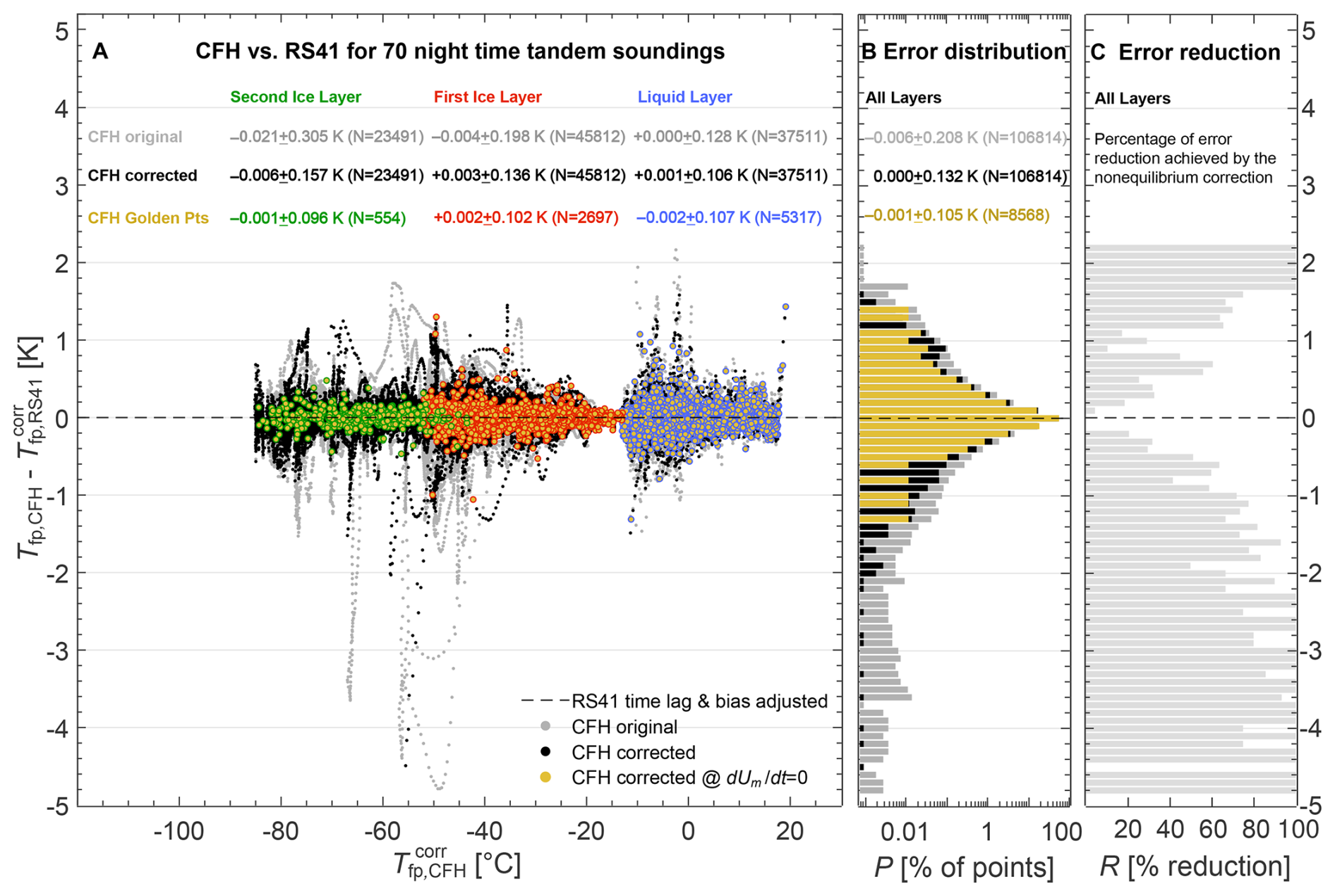
Figure 12 Error statistics based on 106 814 CFH-RS41 tandem measurement data points. (A) Frost point differences (in K) between CFH (denoted by T_fp,CFH) and RS41, which was individually time-lag and bias-corrected by means of the CFH Golden Points $(T_{\mathrm{fp},\mathrm{RS}\mathrm{41}}^{\mathrm{corr}}$), as a function of temperature (a-posteriori minus a-priori). Gray points: uncorrected CFH mirror temperature ($T_{\mathrm{fp},\mathrm{CFH}}=T_{\mathrm{m}}$). Black points: nonequilibrium-corrected CFH (T_fp,CFH = $T_{\mathrm{fp},\mathrm{CFH}}^{\mathrm{corr}}$). Yellow circles with colored borders: CFH Golden Points for the different condensate types (liquid film blue, first ice film red, second ice film green). Text inserts: mean values ± standard deviations for each data type T_fp,CFH and each type of condensate. (B) Probability distribution of frost point differences (in K) across all condensate types for original data (gray), nonequilibrium-corrected data (black), and Golden Points (yellow). Each bar in the histogram represents the occurrence probability in a 0.1 K interval. (C) Reduction of the probability of a given error to occur in percent calculated as ratio of the occurrence with and without nonequilibrium correction $R=\mathrm{1}-P(T_{\mathrm{fp},\mathrm{CFH}}^{\mathrm{corr}}-T_{\mathrm{fp},\mathrm{RS}\mathrm{41}}^{\mathrm{corr}})/P(T_{\mathrm{m}}-T_{\mathrm{fp},\mathrm{CFH}}^{\mathrm{corr}})$.

The text insert in Fig. 12 lists individually for all three condensate types the mean bias and standard deviation, corresponding to the root mean square error (RMSE) between corrected RS41 and CFH (original, corrected and Golden Points). For the second ice layer (UT/LS) the nonequilibrium correction achieves about 45 % reduction in RMSE, for the first ice layer 30 % reduction, and for the liquid layer about 20 % reduction. Interestingly, there are a few Golden Points with $|T_{\mathrm{fp},\mathrm{CFH}}-T_{\mathrm{fp},\mathrm{RS}\mathrm{41}}^{\mathrm{corr}}|$ > 1 K, while one might expect this to be smaller than the uncertainty of 0.2 K. However, we first note the fitting procedure for each condensate film with two parameters for the time-lag correction and six parameters for the bias correction leaves some room for outliers, whereas the vast majority of Golden Points deviates less than 0.2 K (see logarithmic bar diagram in Fig. 12B). For the liquid film the nonequilibrium correction is the least efficient and the RMSE at the Golden Points is the largest. Despite the time-delay correction in the optimization routine described in Appendix B, the ±1 s uncertainty in sampling the Golden Points likely plays a bigger role for the liquid film, as CFH typically oscillates much more strongly (i.e. large $|\mathrm{d}{T}_{\mathrm{m}}/\mathrm{d}t|$ at the Golden Points). In addition, the noise in the resistance measurement induces a small random uncertainty in the lower troposphere (Sect. 2.5).

Figure 12B depicts the logarithmically plotted distribution of CFH-RS41 errors across all condensate types, demonstrating the effectiveness of the nonequilibrium correction (change from gray to black histogram) and the superior quality of the Golden Points (yellow histogram). In particular, note the effectiveness in eliminating most of the extremely dry outliers, i.e. some layers of extreme-low bias can be identified and corrected, which is important for trend detection. The figure also reveals that nonequilibrium errors do not affect measurement accuracy when averaged over a large number of soundings (−6 mK bias over all soundings over all layers), which is indicative of appropriate PID control on average, as noted also in Vömel et al. (2016).

For CFH, the combined effect of all sources of uncertainty in frost point (or dew point) measurements is specified to be better than 0.2 K under good conditions, and systematic errors, which most likely affect long-term climate series, are smaller than 0.1 K (Vömel et al., 2016). Figure 12 confirms this performance for a majority of 89 % of the measurement points. For 11 % of the about 10⁵ measurement points, the nonequilibrium analysis revealed errors in the frost point estimated from the raw mirror temperature (i.e., $|T_{\mathrm{m}}-T_{\mathrm{fp},\mathrm{RS}\mathrm{41}}^{\mathrm{corr}}|$) of more than 0.2 K, for 5.5 % of more than 0.3 K, for 2.2 % of more than 0.5 K, and for 0.6 % larger of more than 1.0 K. For the subset of points with the second ice film (near the tropopause, about 23 000 points), 37 % have errors in frost point larger than 0.1 K, 18 % larger than 0.2 K, 10 % larger than 0.3 K, 4 % larger than 0.5 K, and 1 % larger than 1.0 K. As mentioned earlier, because of different ice film qualities not all instruments or flight legs are equally affected by nonequilibrium errors. Since 40 of the 70 analyzed soundings have been launched from Lindenberg under the optimal launch conditions at the GRUAN Lead Center and the moderate midlatitude flight conditions, these statistics might be slightly worse for other stations and flight campaigns with lower H₂O mixing ratio, such as in the tropical UT/LS. In fact, for the subset of points with the second ice film (near the tropopause), only 32 % of all flights have errors in frost point < 0.2 K (for at least 95.4 % of their measurements points). All of these flights achieving this level of performance were launched from Lindenberg, where about $\mathrm{2}/\mathrm{3}$ of the flights satisfy the < 0.2 K criterion.

7 Conclusions

This study shows how measurements with errors in the frost point > 0.2 K from reference quality chilled mirror hygrometers, such as CFH, are caused by controller instabilities leading to nonequilibrium states of the chilled mirror, and how they can be systematically corrected. Measurements by chilled mirror hygrometers are a composite of oscillating mirror temperature T_m and mirror reflectance U_m signals. Oscillations around the dew/frost point are inherent to the chilled mirror measuring technique and cannot be avoided. Regardless of the control approach, the H₂O partial pressure can be calculated according to the nonequilibrium equation $p_{\mathrm{vap}}\left(T_{\mathrm{m}}\right)-p_{\mathrm{vap}}\left(T_{\mathrm{fp}}\right)\propto (p/A^{\prime })\cdot (\mathrm{d}{U}_{\mathrm{m}}/\mathrm{d}t)$ (Eq. 5).

7.1 Golden Points: most accurate chilled mirror data

A fundamental characteristic of chilled-mirror hygrometers that the actual dew/frost point is only measured when the condensate (liquid water or ice) is in equilibrium with the ambient gas phase, i.e. at the Golden Points ($\mathrm{d}{U}_{\mathrm{m}}/\mathrm{d}t$ = 0). For CFH, the 2σ uncertainty is less than 4 % in the mixing ratio at the Golden Points. Away from the Golden Points, when the condensate is not in equilibrium ($\mathrm{d}{U}_{\mathrm{m}}/\mathrm{d}t\ne \mathrm{0}$), the measurement error is proportional to the change in mirror reflectivity per time, independently of the controller action. When the reflectance increases, the condensate is evaporating and the mirror is too warm. Conversely, when the reflectance decreases, the condensate is growing and the mirror is too cold. The Golden Points are a powerful feature of chilled mirror hygrometers as they provide physical confirmation of thermodynamic equilibrium (or equilibrium-like points in time). As such, they strengthen the use of chilled mirror hygrometers as reference instruments with high accuracy and negligible drift, suited for long-term records of H₂O in the upper troposphere and lower stratosphere.

7.2 Nonequilibrium correction: H₂O profiles of improved accuracy and vertical resolution

Correcting the nonequilibrium states of CFH requires an estimate of the morphological sensitivity A^′, which contains information about the frost (or dew) morphology on the mirror. When CFH is flown together with a second humidity sensor with potentially lower accuracy but a temporal resolution better than the spacing of the Golden Points, this sensor can first be recalibrated using the accurate CFH Golden Points, and then the recalibrated sensor can in turn be used to correct the nonequilibrium states of CFH. Such a second sensor can be a high-performance thin film sensor like the RS41 or an optical hygrometer like FLASH-B. Except for contaminated flights (hydrometeors in the inlet or outgassing of the balloon envelope), we found from 70 night time soundings that the non-equilibrium correction achieves a 60 %–100 % reduction in the frost point error for errors greater than 1 K, provides a significant improvement in measurement accuracy for 68 % of the flights, and results overall in a 2σ uncertainty of less than 0.4 K at a vertical resolution of 125 m or less than 0.2 K (i.e., 4 % in the mixing ratio) at 500 m vertical resolution from the ground to the middle stratosphere. This shows that the target uncertainty of < 4 % in the mixing ratio set by the WMO in 2024 is achievable when applying a nonequilibrium correction. The method achieves higher accuracy and vertical resolution, and is less prone to outliers, than traditional averaging techniques (that do not account for the mirror reflectance) for cooling mirror devices such as CFH, for which a 2σ uncertainty of 10 % in the mixing ratio is specified. Attempts to consider chilled mirror instruments as time-lagged (i.e. following a first-order response with time constants of several seconds), as found sometimes in literature, are generally inappropriate, because chilled mirrors are actively controlled devices and usually follow a higher order response with multiple overshoots. Furthermore, attempts to remove nonequilibrium errors with downsampling techniques or low-pass filtering over several hundreds of meters are prone to bias in case of large and/or asymmetric nonequilibrium errors, and reduce vertical resolution.

Self-correction: Under suitable circumstances, a nonequilibrium correction can be applied without the use of an auxiliary humidity sensor. One approach is to derive an a-priori profile from an array of closely spaced Golden Points with mirror temperature oscillations of sufficiently large amplitude in-between, given the Golden Points positions can be determined precisely. Another approach is to derive the morphological sensitivity by matching ascent and descent data in the stratosphere, given the presence of atmospheric/non-atmospheric features in regions of moderate enough flow rate.

7.3 Recommendations for future instrumentations and data treatment

Looking ahead, it would be interesting to investigate new hygrometer designs that make optimal use of the Golden Points concept. In particular, feedback control could be improved in two ways: minimize nonequilibrium errors such that a nonequilibrium correction is not required, or enable robust nonequilibrium self-correction.

Improved PID controller to minimize nonequilibrium errors: it is now clear that the error remains small, $|T_{\mathrm{m}}-T_{\mathrm{fp}}|\propto |\mathrm{d}{U}_{\mathrm{m}}/\mathrm{d}t|/A^{\prime }$ < 0.2 K (Eq. 8a), when the morphological sensitivity A^′ is large and the change in reflectivity $|\mathrm{d}{U}_{\mathrm{m}}/\mathrm{d}t|$ is small, ideally in conjunction with sufficiently frequent Golden Points and an average nonequilibrium error remaining close to zero along the flight path (see Fig. 7A–B for examples with Golden Points every ∼ 150 m). Maximizing A^′ through an improved mirror design, such as a hydrophilic micropattern structure printed or deposited on the mirror, could increase the consistency and morphological sensitivity of the mirror condensate. Furthermore, the introduction of an adjustable setpoint could help reduce non-equilibrium deviations and thus improve the performance of chilled mirror hygrometers.

Improved PID controller for self-correction ability: a-priori profiles can be derived from dense arrays of Golden Points and quasi-symmetric mirror temperature oscillations of sufficiently large amplitude. The timing of the Golden Points is particularly important in such an approach. New designs with live detection of the Golden Points by a microcontroller (i.e., sampling T_m and U_m at an internal rate ≫ 1 Hz and transmission of the data in telemetric batches) could reduce the uncertainty of the Golden Points positions and be useful for sensors with large $|\mathrm{d}{U}_{\mathrm{m}}/\mathrm{d}t|$, provided any time lag between U_m and T_m can be well characterized. Enforcing mirror temperature oscillations at a fixed frequency (e.g., $\mathrm{1}/\mathrm{60}$ Hz) and suppressing this artificial, non-atmospheric frequency in the non-equilibrium-corrected data could be another promising approach to the Golden Points.

Data archive: correction for nonequilibrium requires the composite T_m and U_m chilled mirror signal, we therefore recommend reporting both T_m and U_m in chilled mirror data products (e.g., from NDACC). The U_m signal is also important for data quality check.

Appendix A: Flights Table

Table A1 Compilation of the CFH soundings examined in this work. Rows 71–75 list experimental flights discussed in the paper which have not been included in the statistical analysis in Sect. 6.

Appendix B: Vaisala RS41 capacitive thin-film polymer sensor

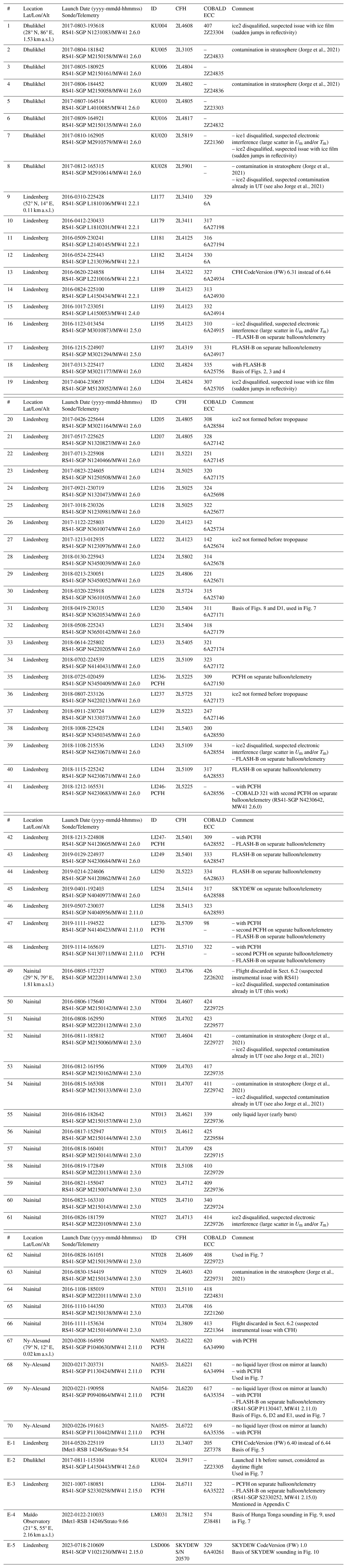
RS41 is an operational radiosonde manufactured by Vaisala (Vaisala, 2018a, b) and the successor of RS92 (Vaisala, 2013), see also (Nash et al., 2011; Dirksen et al., 2024). The performance of radiosondes has greatly improved since Elliott and Gaffen (1991) questioned their usefulness for climate studies. The capacitive thin-film humidity sensor of the Vaisala RS41 radiosonde, for example, remains sensitive to humidity as long as the relative humidity is greater than about 1 %–2 % RH (Survo et al., 2015; Vömel et al., 2022; Khaykin et al., 2022). This suggests that it can be utilized within certain UT/LS research topics, such as the study of deep overshooting convection, polar stratospheric clouds or moist volcanic plumes. However, in the tropopause region and in the stratosphere the RS41 (with the Vaisala MW41 sounding software) may exhibit residual time-lag and bias errors that can result in errors of 20 % of more (e.g. Brunamonti et al., 2019; Khordakova et al., 2022), which can be improved using a universal correction (Poltera, 2022). In addition, there is sonde-to-sonde variability, which introduces additional uncertainty in the low humidity regime of the tropopause region and the stratosphere (Brunamonti et al., 2019; Vömel et al., 2022). Nevertheless, the RS41 measurements can be time-lag and bias-corrected to match the CFH Golden Points on a case-by-case basis. This allows constructing an a-priori estimate for the nonequilibrium correction of CFH. In addition, it provides information on the behavior of the RS41 humidity sensor in environments that are challenging to reproduce in the laboratory, such as the UT/LS.

B1 Using a recalibrated RS41 for the nonequilibrium correction of CFH

Using an RS41 as auxiliary sensor, we apply the nonequilibrium correction procedure described in Sect. 4.2 according to the following scheme:

1. identify the Golden Points along the humidity profile measured by CFH;

2. construct an a-priori estimate of the frost point profile by means of an RS41 on the same balloon payload, which is

   • synchronized to the CFH telemetry (i.e. correcting for a mismatch of typically about Δ_tele = 3.5 s (Holger Vömel, personal communication, 2019; Poltera, 2022);

   • time-lag-corrected by means of a 2-parameter Arrhenius-type equation ($\sim \exp (\mathrm{\Delta }E/RT)$) for the time constant, see Eq. (B1);

   • and bias-corrected by means of the Golden Points of the chilled mirror instrument using 6 parameters (in the form of an offset and a scaling-factor), see Eq. (B2);

3. use this a-priori estimate to determine the effective sensitivity A of CFH;

4. construct an a-posteriori by correcting the CFH mirror temperature using A in Eq. (8a), called “nonequilibrium corrected CFH”.

The a-posteriori is our best approximation for the “true” frost point. We use the deviation between the a-priori and the a-posteriori as an estimate of the uncertainty of the frost point resulting from residual errors in the nonequilibrium correction of CFH and in the time-lag and bias correction of the RS41 data based on the CFH Golden Points.

B2 Time-lag correction for RS41

The RS41 humidity measurement can be used to construct the CFH nonequilibrium correction, even though it is often less accurate in the upper troposphere and in the stratosphere (e.g. Brunamonti et al., 2019; Sun et al., 2021; Lee et al., 2021; Khordakova et al., 2022) and fails to reproduce the CFH Golden Points, as shown by the green dashed in Fig. 2A. Therefore, RS41 must first be corrected for time-lag and bias by means of the Golden Points, before it can be used to correct the nonequilibrium states of CFH. This utilizes the high precision of the corrected RS41 data.

The capacitive RS41 humidity sensor operates on the principle of the change in the electrical capacitance of a thin polymer film due to moisture absorption. When atmospheric humidity changes, the H₂O molecules must diffuse into or out of the polymer film, which takes time, causing the sensor to react with a diffusive delay and with a damped response to changes in the external humidity. This is best described by in terms of an Arrhenius-type temperature dependence (e.g. Denton et al., 1985) of the characteristic time for diffusion through the layer

$$\begin{array}{}\text{(B1)}& {\mathit{\tau }}_{\mathrm{RS}\mathrm{41}}\left(T\right)={\mathit{\tau }}_{\mathrm{\infty }}\cdot \exp \left({\displaystyle \frac{E_{\mathrm{a}}}{R{T}_{\mathrm{RS}\mathrm{41}}}}\right),\end{array}$$

where τ_RS41 is the corresponding time constant, T_RS41 is the temperature of the RS41 humidity sensor in K (aimed to be at 5 K above ambient temperature), E_a is the diffusion activation energy (in J mol⁻¹) and τ_∞ is a pre-factor (in s). The Arrhenius description ($\sim \exp (\mathrm{\Delta }E/RT)$) captures the physics of the instrument better than a polynomial dependence on temperature, as previously assumed by Miloshevich et al. (2004) or a simple exponential dependence ($\sim \exp (-cT)$) used by Vaisala (Antikainen and Paukkunen, 1994) and the research community (Leiterer et al., 2005; Dirksen et al., 2014). In particular, at low temperatures, the Arrhenius dependence provides a more realistic description and appears to better reproduce recent laboratory measurements at temperatures lower than previously tested (Von Rohden et al., 2021, 2022; see also Dirksen et al., 2020). Since E_a and τ_∞ may vary slightly between different copies of RS41 due to small differences in design, such as film thickness, we fit Eq. (B1) individually for each flight segment along with other parameters and use this to correct RS41 for its time-lag. The equation for time-lag deconvolution is found in Miloshevich et al. (2004), their Eq. (4).

B3 Bias correction for RS41

The bias is corrected by means of the 6-parameter fit mentioned in Sect. 3.2, namely in terms of an offset S₀ and a scaling factor ξ, following the rationale of the correction of the temperature dependence in ice chamber laboratory experiments applied by Vaisala to their radiosonde humidity sensors in the past (Wang et al., 2002; Miloshevich et al., 2001, 2004):

$$\begin{array}{}\text{(B2)}& \begin{array}{rl}{S}_{\mathrm{corr}}\left(S,T\right)=& \left(S-S_{\mathrm{0}}\right)\times \mathit{\xi }\\ =& \left(S-\left(a_{\mathrm{0}}+a_{\mathrm{1}}{T}_{\mathrm{RS}\mathrm{41}}+a_{\mathrm{2}}{T}_{\mathrm{RS}\mathrm{41}}^{\mathrm{2}}\right)\right)\\ & \times \left(b_{\mathrm{0}}+b_{\mathrm{1}}{T}_{\mathrm{RS}\mathrm{41}}+c_{\mathrm{0}}\cdot S\right),\end{array}\end{array}$$

where S is the H₂O saturation ratio (with respect to liquid water or ice, depending on the condensate on the mirror) measured with RS41 (after time-lag correction), T_RS41 is the measured temperature of the RS41 humidity sensor, and a_i, b_i and c₀ are six bias correction parameters. Equation (B2) is also fitted individually for each flight segment together with other parameters and this is used to correct RS41 for its bias.

B4 Details of the implementation of the nonequilibrium correction

To account for changes of the film morphology after each cleaning cycle of each sounding, we subdivide each flight into three segments: the liquid film segment (from balloon launch to the first CFH cleaning cycle at T_m = −15 °C), the segment with the first ice film (from the first to the second cleaning cycle), and the segment with the second ice film (from the second cleaning cycle at T_m = −53 °C to the hygropause). We conservatively limit the analysis to below the hygropause, since the detection limit of 1 %RH–2 %RH of the RS41 polymer humidity sensor (e.g. Brunamonti et al., 2019; Vömel et al., 2022) was reached just above the hygropause in some of the Lindenberg flights and because the uncertainty of the time-lag correction of capacitive thin-film sensors is greatest during desorption from the thin-film polymer in the first kilometers above the hygropause (Dirksen et al., 2014). Therefore, nonequilibrium correction above the hygropause in the stratosphere must rely on the nonequilibrium parameters obtained in the upper troposphere below the hygropause, which is justified as long as the morphology of the ice film does not change during further ascent.

For each flight segment (liquid film, first ice film, and second ice film until the tropopause), we extract the local minima and maxima after smoothing the reflectance signal (3-point half-width second-order Savitzky-Golay filter for the liquid film, 5-point for the first ice film, and 15-point for the second ice film). This filter aims to reduce random noise (e.g., microscopic fluctuations in ice crystal shape and size, stray light from the ambient or from the instrument's light source, and noise of the electronics), while not causing a time shift, i.e. keeping the Golden Points at their original position in the profile. To avoid local extremes due to noise, neighboring maxima and minima are required to differ from each other by at least 3 % of the range of all reflectance values in the flight segment. Golden Points and portions of flight segments where the mirror is suspected to be blank or contains only very little condensate are discarded (i.e., the reflectance must be smaller than U_m = 2.5 V + 0.95 ⋅ (U_m,clean − 2.5 V), where U_m,clean is the signal value of the blank mirror determined during instrument preparation).

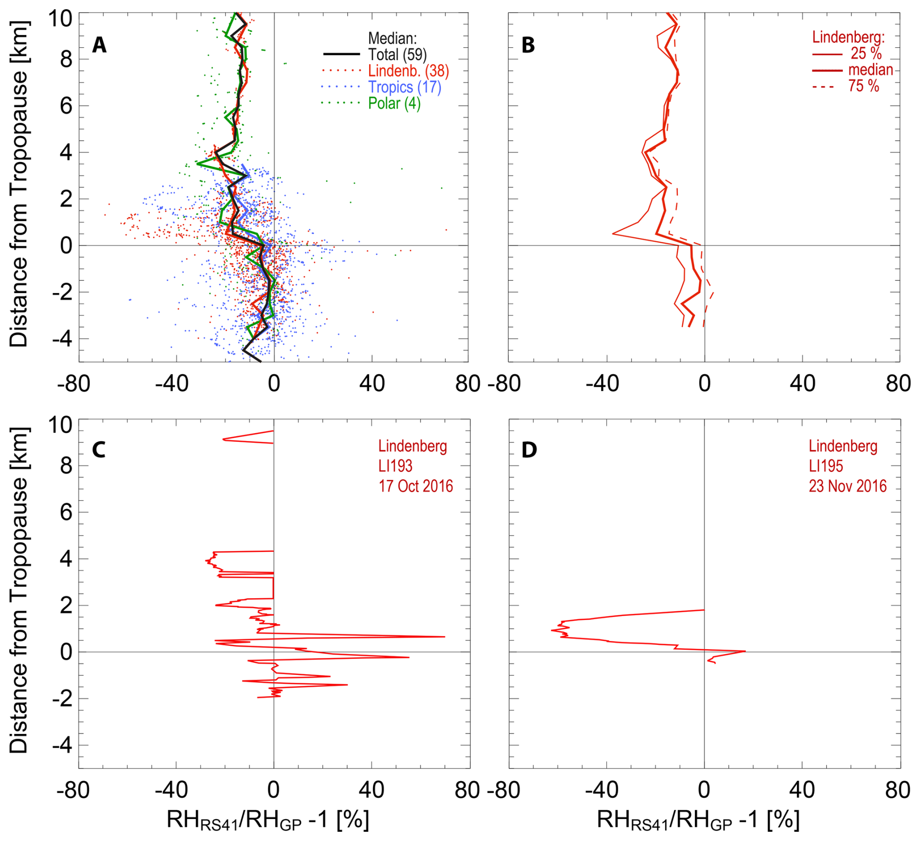
Figure B1 Comparison of (RH_RS41 − RH_GP) $/$ RH_GP of the RS41 manufacturer product with 3042 Golden Points (GP) of CFH. The GP have an uncertainty of 0.2 K in the frost point corresponding to an uncertainty of less than 3.5 % in the value of RH. (A) Scatter plot of (RH_RS41 − RH_GP) $/$ RH_GP for 3042 GP during 59 RS41-CFH tandem soundings after the second cleaning cycle (i.e., second ice film). These are the soundings listed in Table A1, excluding flights with apparent contamination problems. Launch sites are color coded. Lines show median values in 500 m steps. (B) 25 %, 50 %, and 75 % percentiles for the 38 soundings from Lindenberg, showing the reduced RS41 data quality with a pronounced dry bias directly above the tropopause and larger sonde-to-sonde variability. (C, D) Two examples of Lindenberg soundings illustrating the RS41 sonde-to-sonde-variability.

We then employ a numerical optimization solver (Storn and Price, 1996) to adjust the RS41 data to best match the CFH Golden Points. This involves fitting nine correction parameters for the RS41:

• the two time-lag correction parameters τ_∞ and E_a (Eq. B1);

• six bias correction parameters a₀, a₁, a₂, b₀, b₁, c₀ (Eq. B2);

• the width of a boxcar filter for flight segments with ice, N_boxcar, that is used to smooth the CFH and RS41 relative humidity data in the same manner;

• a time-delay parameter for flight segments with liquid condensate, Δ_delay, which accounts for any sub-second mismatch in time between mirror temperature and reflectance.

The solver is given lower and upper bounds for each of the parameters (Poltera, 2022, Table A.1), and then searches for the parameters that best align the RS41 with the CFH data at all Golden Points within the flight segment. In the solver, the RS41 raw data of RH (at the humidity sensor temperature) is first time-lag corrected (as in Miloshevich et al., 2004) and then smoothed with the boxcar filter. The resulting smoothed RH profile is then bias-corrected and transformed to frost point. The CFH mirror temperature is first converted to RH to be comparable with the RS41 measurements; then the CFH RH is synchronized (sub-second time shifted) with RS41 by means of Δ_delay (after Δ_tele has been taken into account), smoothed with the same boxcar filter as the RS41, then transformed back to frost point. The formulation by Murphy and Koop (2005) is used for the saturation vapor pressure over ice, and the ITS-90 compatible form of Wexler's formulation (Hardy, 1998) for the saturation vapor pressure over water, which is the saturation vapor pressure of liquid water used by Vaisala for the RS41 (Survo et al., 2014). For air pressure, the RS41 GPS-based data product from Vaisala is used. The solver minimizes the RMSE (or, equivalently, the standard deviation) between the corrected RS41 frost point ($T_{\mathrm{fp},\mathrm{RS}\mathrm{41}}^{\mathrm{corr}}$) and the CFH frost point (T_m) at the location of the CFH Golden Points.

For flight segments with ice films, we prescribe Δ_delay = 0, while for flight segments with liquid films we prescribe N_boxcar = 1, because sub-second delay errors are less significant than time-lag errors at lower temperatures, while the opposite is true at higher temperatures. The solver is used to fit the remaining 9 parameters simultaneously to obtain the best match with the CFH Golden Points. From the 70 soundings discussed in Sect. 6, the residual fitting error (RMSE) is 0.1 K (1σ) for the Golden Points. After that, the derived corrected frost point $T_{\mathrm{fp},\mathrm{RS}\mathrm{41}}^{\mathrm{corr}}$ serves as the atmospheric reference frost point profile, from which we derive the effective sensitivity parameter A of CFH by minimizing the residual error of Eq. (8b), i.e. of $A\cdot \left(T_{\mathrm{m}}\right(t)-T_{\mathrm{fp},\mathrm{RS}\mathrm{41}}^{\mathrm{corr}}(t\left)\right)=B\left(t\right)\cdot \mathrm{d}{U}_{\mathrm{m}}/\mathrm{d}t\left(t\right)$.

B5 RS41 performance in the UT/LS

Figure B1 demonstrates that residual time-lag and bias errors, along with increasing sonde-to-sonde variability, reduce the accuracy of RS41 measurements in the stratosphere.

Appendix C: The Lyman-α hygrometer FLASH-B

FLASH-B (Fluorescent Lyman-α Stratospheric Hygrometer for Balloon) is a compact light-weight balloon-borne hygrometer for the upper troposphere and the stratosphere manufactured by CAO (Central Aerological Observatory, Russia; Yushkov et al., 1998, 2001; Lykov et al., 2011). It is based on the Lyman-α fluorescence technique for fast measurements of low concentrations of water vapor (Kley and Stone, 1978; Bertaux and Delannoy, 1978). FLASH-B measures in open configuration with downward-facing optics. Measurements are only possible at night to protect the instrument's photocathode, and during ascent outgassing typically restricts the validity of the measurements up to the tropopause region (Ghysels et al., 2016). The measuring range is 0.5–1000 ppmv at pressures between 5 and 300 hPa. At higher atmospheric pressure, Lyman-α absorption by H₂O vapor becomes significant and in the lower troposphere fluorescence counting is strongly attenuated, which is a general limitation of the Lyman-α fluorescence method and not specific to FLASH-B (Kley and Stone, 1978; Bertaux and Delannoy, 1978). The overall calibration error is estimated to be 4 % (1σ), and the measurement accuracy for a fluorescence signal integrated over 4 s is typically 5.5 % under stratospheric conditions. The overall uncertainty (1σ) is < 10 % for H₂O mixing ratios of more than 3 ppmv and < 20 % below 3 ppmv (e.g. Vömel et al., 2007b; Lykov et al., 2011; Lykov and Khaykin, 2017).

The performance of FLASH-B has been assessed in the laboratory during the AquaVIT-1 hygrometer intercomparison campaign (Fahey et al., 2014) in the stratospheric chamber AIDA in Karlsruhe (Germany), and in the atmosphere by comparisons with the MIAWARA microwave radiometer (Deuber et al., 2005), the FPH (Vömel et al., 2007b) and CFH (Khaykin et al., 2013) chilled mirror hygrometers, and against the tunable diode laser IR-absorption spectrometer Pico-SDLA H₂O (Ghysels et al., 2016). These comparisons showed average relative deviations less than 2.4 % in the lower stratosphere (Kalnajs et al., 2021), which is well within the instrumental uncertainties of the instruments involved. Similar to FLASH-A, the aircraft version of the instrument, also the balloon version is not an absolute water vapor instrument and requires to be recalibrated between flights, with the challenge being the long-term stability of the UV-light source and the aging of the MgF₂ window (Meyer et al., 2015), as well as possible interferences, such as stray-light interference (e.g. Sitnikov et al., 2007) or an offset in fluorescence counts (Poltera, 2022), see below.

C1 Using a recalibrated FLASH for the nonequilibrium correction of CFH

With its fast response and a measurement precision of about 5.5 %, FLASH-B is particularly suited for the study of fine-scale processes in the UT/LS and stratosphere, such as horizontal moisture transport and overshooting convection in the tropics (Khaykin et al., 2009, 2016; Liu et al., 2010), or water vapor (re-)distribution and PSC-dehydration in the Arctic (Maturilli et al., 2006; Karpechko et al., 2007; Lukyanov et al., 2009; Khaykin et al., 2013; Engel et al., 2014). The calibration procedure is described by Vömel et al. (2007b) and Lykov et al. (2011). Calibration is performed at CAO (Central Aerological Observatory, Russia), or, if the station has the necessary calibration equipment, such as the Lindenberg Observatory, directly at the sounding station (Lykov and Khaykin, 2018). Alternatively, in-flight calibration by comparing the FLASH-B fluorescence counts with an accurate estimate of the water vapor mixing ratio at 50 hPa (e.g. from CFH or Aura/MLS) during balloon descent (Sergey Khaykin, personal communication, 2021), or at 300 hPa (e.g. from CFH or RS41) during balloon ascent (Peter Oelsner, personal communication, 2022) is also possible. Large discrepancies (Dirksen, 2020) between pre-flight calibration coefficients derived in the laboratory and in-flight calibration coefficients derived from comparison with RS41 and CFH can be explained by a constant offset in fluorescence count rate (Poltera, 2022). As an example, although the accuracy of the original FLASH-B measurement cannot reproduce the CFH Golden Points, as shown by the green dashed line in Fig. 2B, the FLASH humidity measurement can be used to construct the CFH nonequilibrium correction by means of the introduction of an offset in fluorescence count rate (see Fig. 4). This requires fewer recalibration parameters than the RS41 recalibration (2 vs. 10) and without residual time-lag uncertainty, since FLASH is an optical measurement.

C2 Offset-correction of FLASH

While it is known (Sitnikov et al., 2007) that the airplane version of the instrument, FLASH-A, which resides in a closed compartment, must be corrected for stray light, which results in an offset, the balloon instrument measures in an open configuration with downward-facing optics. Therefore, no offset is expected for FLASH-B (Fahey et al., 2014). However, the offset estimated in Sect. 3.2 (78.5 counts s⁻¹) must be considered appropriate for that particular flight, as also confirmed by a FLASH PI (Sergey Khaykin, personal communication, 2021). This suggests that the standard calibration of FLASH-B, which assumes a simple proportionality of H₂O mixing ratio and count rate at 50 hPa, was inadequate for the measurements shown in Fig. 2. We identified two other flights where offset corrections of the fluorescence signal were required, albeit to a much lesser extent than in Fig. 2 (about 2.5 counts s⁻¹ (with calibration constant 0.1812 ppmv (counts s⁻¹)⁻¹) for the FLASH instrument “FI07/49” flown in Ny-Ålesund on 21 February 2020, and about 27.1 counts s⁻¹ (with calibration constant 0.0318 ppmv (counts s⁻¹)⁻¹) for “FI05/16” on 7 October 2021, in Lindenberg, resulting in errors of up to 10 % and 20 %, respectively, see Fig. 3.9 of Poltera, 2022). Nevertheless, it is currently unclear whether an offset correction is only required for certain specimens of this instrument or is a general property of FLASH-B.

The original FLASH-B equation (Lykov et al., 2017; Lykov and Khaykin, 2018) can be extended by introducing a constant offset in fluorescence count rate as additional calibration parameter:

$$\begin{array}{}\text{(C1)}& \begin{array}{rl}S=& S_{\mathrm{offset}}+{\displaystyle \frac{\mathrm{1}}{K_{\mathrm{cal}}}}\cdot T_Q\left(p,T\right)\cdot T_{{\mathrm{H}}_{\mathrm{2}}\mathrm{O}}({\mathit{\chi }}_{{\mathrm{H}}_{\mathrm{2}}\mathrm{O}},p,T)\\ & \cdot T_{{\mathrm{O}}_{\mathrm{2}}}\left(p,T\right)\cdot {\mathit{\chi }}_{{\mathrm{H}}_{\mathrm{2}}\mathrm{O}},\end{array}\end{array}$$

where S is the fluorescence counts signal (in counts s⁻¹) and ${\mathit{\chi }}_{{\mathrm{H}}_{\mathrm{2}}\mathrm{O}}$ is the H₂O mixing ratio. The O₂ and H₂O Beer-Lambert transmission terms satisfy $\ln \left(T_{{\mathrm{O}}_{\mathrm{2}}}\right)=-{\mathit{\sigma }}_{{\mathrm{O}}_{\mathrm{2}}}\cdot \mathrm{0.21}\cdot n_{\mathrm{air}}\cdot L$ and $\ln \left(T_{{\mathrm{H}}_{\mathrm{2}}\mathrm{O}}\right)=-{\mathit{\sigma }}_{{\mathrm{H}}_{\mathrm{2}}\mathrm{O}}\cdot {\mathit{\chi }}_{{\mathrm{H}}_{\mathrm{2}}\mathrm{O}}\cdot n_{\mathrm{air}}\cdot L$, where $n_{\mathrm{air}}=p/\left(k_{\mathrm{B}}T\right)$ is the air molecule number density and 0.21 is the mixing ratio of oxygen. The effective Lyman-α absorption cross sections ${\mathit{\sigma }}_{{\mathrm{O}}_{\mathrm{2}}}$ and ${\mathit{\sigma }}_{{\mathrm{H}}_{\mathrm{2}}\mathrm{O}}$ (i.e., the convolution of the line-shape emission of the lamp and the molecular absorption cross sections of O₂ and H₂O) and the Lyman-α absorption path length L for FLASH-B are ${\mathit{\sigma }}_{{\mathrm{O}}_{\mathrm{2}}}$ = 1.00985 × 10⁻²⁰ cm², ${\mathit{\sigma }}_{{\mathrm{H}}_{\mathrm{2}}\mathrm{O}}$ = 1.4552 × 10⁻¹⁷ cm² and L = 5 cm. The quenching term is $T_Q(p,T)=Q(p,T)/Q(\mathrm{1000}\mathrm{hPa},\mathrm{0}\mathit{°}\mathrm{C})$, where $Q(p,T)=n_{\mathrm{air}}/(\mathrm{1}+n_{\mathrm{air}}\cdot k_{q,\mathrm{air}}/A_{\mathrm{0},\mathrm{0}})$ with quenching rate coefficient k_q,air and the Einstein transition probability A_0,0 taken as k_q,air = 2.3 × 10⁻¹¹ cm³ s⁻¹ and A_0,0 = 1.26 × 10⁶ s⁻¹ (Lykov et al., 2017). Equation (C1) has been solved by an approximate fit by Lykov et al. (2017), which limits the applicability to p < 300 hPa. However, Eq. (C1) has an analytical solution, which extends the range of applicability to about p < 500 hPa:

$$\begin{array}{}\text{(C2)}& \begin{array}{rl}{\mathit{\chi }}_{{\mathrm{H}}_{\mathrm{2}}\mathrm{O}}=& -{\displaystyle \frac{\mathrm{1}}{{\mathit{\sigma }}_{{\mathrm{H}}_{\mathrm{2}}\mathrm{O}}\cdot n_{\mathrm{air}}\cdot L}}\\ & \cdot W_{\mathrm{0}}\left(-{\displaystyle \frac{{\mathit{\sigma }}_{{\mathrm{H}}_{\mathrm{2}}\mathrm{O}}\cdot n_{\mathrm{air}}\cdot L}{T_Q\cdot T_{{\mathrm{O}}_{\mathrm{2}}}}}\cdot K_{\mathrm{cal}}\cdot \left(S-S_{\mathrm{offset}}\right)\right),\end{array}\end{array}$$

where W₀(x) is the 0th (i.e. principal/upper) branch of the Lambert W-function, which solves $W_{\mathrm{0}}\left(x\right)\cdot \exp \left(W_{\mathrm{0}}\right(x\left)\right)=x$ (Poltera, 2022). The solution for the upper branch W₀ of the Lambert W-function is only valid when $W_{\mathrm{0}}\left(x\right)\ge -\mathrm{1}$ and $x\ge -e^{-\mathrm{1}}$, i.e. when ${\mathit{\chi }}_{{\mathrm{H}}_{\mathrm{2}}\mathrm{O}}\cdot {\mathit{\sigma }}_{{\mathrm{H}}_{\mathrm{2}}\mathrm{O}}\cdot n_{\mathrm{air}}\cdot L\le \mathrm{1}$ and when $K_{\mathrm{cal}}\cdot (S-S_{\mathrm{offset}})\cdot {\mathit{\sigma }}_{{\mathrm{H}}_{\mathrm{2}}\mathrm{O}}\cdot n_{\mathrm{air}}\cdot L\le e^{-\mathrm{1}}\cdot T_Q\cdot T_{{\mathrm{O}}_{\mathrm{2}}}$.

The FLASH-B calibration parameters K_cal in (counts s⁻¹)⁻¹ and S_offset in counts s⁻¹ can be fitted by Eq. (C2) within the extended measurement range of FLASH-B (p < 500 hPa and ${\mathit{\chi }}_{{\mathrm{H}}_{\mathrm{2}}\mathrm{O}}$ < 1000 ppmv), using a reference water vapor mole fraction ${\mathit{\chi }}_{{\mathrm{H}}_{\mathrm{2}}\mathrm{O},\mathrm{ref}}$. This allows for in-flight calibration of FLASH-B with a tandem hygrometer used as reference. For the soundings shown in Figs. 2 and 4, we have used the tandem CFH water vapor mixing ratio at the Golden Points as reference ${\mathit{\chi }}_{{\mathrm{H}}_{\mathrm{2}}\mathrm{O},\mathrm{ref}}^{\mathrm{Golden}\mathrm{Pts}}$, together with the GPS-based air pressure and temperature measurements of the RS41, and have fitted K_cal = 0.0256 ppmv (counts s⁻¹)⁻¹ and S_offset = 78.5 counts s⁻¹. FLASH does not directly monitor the lamp power, but the PMT voltage, lamp current and internal temperature typically remain very stable during the soundings at air pressures below 500 hPa (as in the sounding on 13 March 2017 shown in Figs. 2 and 4), indicating that the intensity of the hydrogen-glow discharge lamp is stable and justifies the use of a constant value for K_cal. However, the large positive offset of 78.5 counts s⁻¹ required to minimize the RMSE of the fit warrants a brief discussion. Hydrogen-glow discharge lamps with a mixture of hydrogen and helium are known to suffer from interfering light (often termed “stray light” in the literature) of the helium line at 318 nm, which overlaps with the spectrum of measured hydroxyl fluorescence after exposition of the water molecules to Lyman-α radiation. The FLASH-B lamp uses a special MgF₂ window filter aimed at suppressing the 270–320 nm band emission while still allowing 50 % transmission at the 121.6 nm line. Despite the presence of this filter, in a closed chamber with reflecting surfaces, the reflection of light from the helium line introduces an additive offset to the fluorescence signal (Vömel et al., 2007b; Fahey et al., 2014). We speculate that (i) also reflections from surfaces of the FLASH balloon instrument could cause a constant positive offset in the fluorescence counts, resulting in the observed offset, or (ii) the offset originates from the instrument's electronics.

Appendix D: Uncertainty of reflectance and mirror temperature smoothing

In this appendix we first provide details on the uncertainties in determining the Golden Points and the subsequent nonequilibrium correction by means of case studies. Specifically, we show the impact arising from noise suppression when applying different choices of half widths of the Savitzky-Golay filter. In the second part of the appendix, we compare this with the uncertainty determined by low-pass filtering as used by NDACC for their products.

D1 Noise in CFH measurements and smoothing of reflectance data

The determination of the Golden Points and the non-equilibrium correction require a reliable estimate of the derivative of the reflectance signal U_m. Figure D1 shows a stratospheric segment of the sounding from Lindenberg on 20 April 2018. As shown by the Fig. D1A, the 1s reflectance data may contain small regular oscillations, which render the data much too noisy to allow for a meaningful calculation of the derivative $\mathrm{d}{U}_{\mathrm{m}}/\mathrm{d}t$. The 1 s mirror temperature and reflectance data of CFH are strictly anti-correlated (see Fig. D1A, B). This anti-correlation means that it is impossible for the rapid change in mirror temperature to be a response to the rapid change in reflectance. Although the origin of this quasi-5 s oscillation is unclear, it is clearly not an atmospheric feature. A smoothing using a Savitzky-Golay second order filter with a 15 s half width removes most of the ∼ 5 s oscillations but preserves the structure of U_m on a time scale larger than 30 s. This is also confirmed by the Fourier transform of the 1s and smoothed U_m data shown in Fig. D1C. The amplitude of the Fourier transformed U_m data remains almost unchanged for k < 0.03 s⁻¹, whereas the amplitude at higher frequencies (> 0.2 s⁻¹) is removed by 99 %.

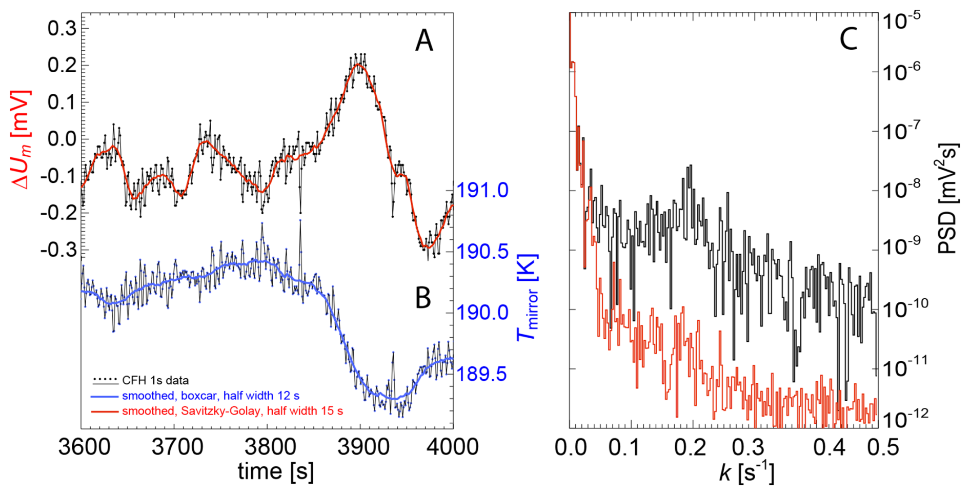
Figure D1 Smoothing of CFH data applied to sounding LI230 (20 April 2018) in Lindenberg (stratospheric segment from 3600 to 4000 s). (A) 1 s mirror temperature data (dots and thin black line) and 25 s boxcar-smoothed mirror temperature. (B) 1 s mirror reflectance data (dots and thin black line) and with Savitzky-Golay filter (15 s half width) smoothed data. (C) Fourier transform of the 1 s (black) and 25 s smoothed (red) reflectance data.

For a sounding in Ny-Ålesund on 21 February 2020 (same as Fig. 6), the influence of smoothing with different widths of the Savitzky-Golay filter is shown for 8 to 10.2 km in Fig. D2. The 1 s U_m data is also clearly too noisy. Conversely, using a very wide Savitzky-Golay filter with half-width of 300 s removes all the structure of mirror reflectance signal, leading to a meaningless effective sensitivity parameter A and $\mathrm{d}{U}_{\mathrm{m}}/\mathrm{d}t$, therefore, no or false non-equilibrium correction. In the end this leads to large deviations (light blue area in Fig. D2C) compared to the results with smoothing by Savitzky-Golay filter width of 7, 15 and 30 s shown by the dark blue area of Fig. D2C.

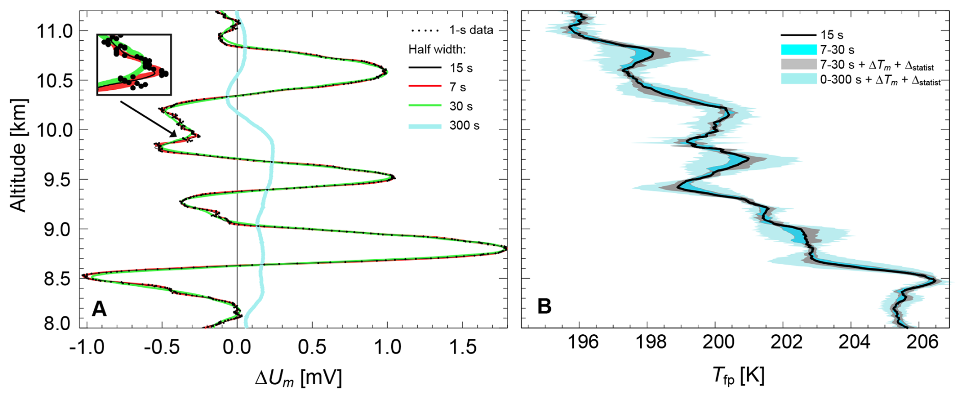
Figure D2 Sensitivity of non-equilibrium correction using different smoothing widths for a sounding in Ny-Ålesund on 21 February 2020 (same as Fig. 6). (A) Reflectance smoothed by using a Savitzky-Golay filter with different widths ranging from 7 to 300 s. (B) The uncertainty of the non-equilibrium corrected CFH frost points. Black line: 15 s filtering. Dark blue shading: range of smoothing of reflectance with 7, 15 and 30 s Savitzky-Golay filter; grey shading: range of smoothing of reflectance with 7–15–30 s Savitzky-Golay plus mirror temperature uncertainty and statistical uncertainty (similarly to NDACC, see also Fig. 6 and Eq. 9); light blue shading: 0–7–15–30–300 s Savitzky-Golay plus mirror temperature and statistical uncertainties.

D2 Uncertainty of low-pass filtering as used by NDACC for their products

Figure 6C shows the low-pass filtered CFH mirror temperature data (T_m) together with its (2σ) total uncertainty for the sounding in Ny-Ålesund (21 February 2020) as archived on NDACC (revision R0). For CFH mirror temperature data archived at NDACC (Revision 0) (2020), the profiles are first flagged for non-valid data (such as cleaning cycles, detachment of pieces of the ice-film and balloon spikes) and the phase of the mirror condensate (liquid water or hexagonal ice) is determined, allowing to calculate the H₂O partial pressure in subsequent processing steps (Vömel et al., 2016, their Appendix A). The mirror temperature is used to calculate the raw H₂O mixing ratio profile, which is then smoothed with a Gaussian filter using a mirror temperature dependent kernel width (Vömel et al., 2016, their Sect. 2.1). The filter is applied on the mixing ratio instead of mirror temperature because it is less bias prone in case of large oscillations (Vömel et al., 2007b). The kernel width is reported in the NDACC data files, and varies typically from 3 s in the lower troposphere to 30 s in the middle stratosphere, which corresponds to an effective vertical resolution of about ($\times (\mathrm{2}\mathit{\pi }{)}^{\mathrm{1}/\mathrm{2}}\times \mathrm{5}$ m s⁻¹) 40 to 400 m (Dirksen et al., 2014, their Eq. A4; Vömel et al., 2016). Flights with good frost control are somewhat finer resolved, e.g., about 165 m at −85 °C mirror temperature (typical lower stratospheric frost point value around 56 hPa or 21 km).

The uncertainty of the downsampled (i.e., Gaussian-smoothed) value, which is the uncertainty of the layer average, is treated similarly as the statistical uncertainty of an average, using a formula adapted for Gaussian kernels (Gatz and Smith, 1995; Vömel et al., 2016). This formula however underestimates uncertainty, because the underlying 1 s data has some degree of auto-correlation due to PID controller oscillations (which are related to the nonequilibrium error described in this paper). For this reason, NDACC increases the uncertainty of the layer average by a scaling factor, which varies somewhat from about 1 at ground to about 3 in the middle stratosphere (Vömel et al., 2016). The (scaled) layer average uncertainty is added in quadrature to 0.11 K (conservative, 1σ) calibration uncertainty, resulting in the total uncertainty of the NDACC frost point product shown in Fig. 6C.