Enhancing Accuracy of Indoor Air Quality Sensors via Automated Machine Learning Calibration

Indoor fine particles (PM_2.5) exposure poses significant public health risks, prompting growing use of low-cost sensors for indoor air quality monitoring. However, maintaining data accuracy from these sensors is challenging, due to interference of environmental conditions, such as humidity, and instrument drift. Calibration is essential to ensure the accuracy of these sensors. This study introduces a novel automated machine learning (AutoML)-based calibration framework to enhance the reliability of low-cost indoor PM_2.5 measurements. The multi-stage calibration framework connects low-cost field sensors to be deployed with intermediate drift-correction reference sensors and a reference-grade instrument, applying separate calibration models for low (clean air environment) and high (pollution events) concentration ranges. We evaluated the framework in a controlled indoor chamber using two different sensor models exposed to diverse indoor pollution sources under uncontrolled natural ambient conditions. The AutoML-driven calibration significantly improved sensor performance, achieving a strong correlation with reference measurements (R² > 0.90) and substantially reducing error metrics (with normalized root-mean-square error (NRMSE) and symmetric mean absolute percentage error (sMAPE) roughly halved relative to uncalibrated data). Bias was effectively minimised, yielding calibrated readings closely aligned with the reference instrument. These findings demonstrate that our calibration strategy can convert low-cost sensors into a more reliable tool for indoor air pollution monitoring. The improved data quality supports atmospheric science research by enabling more accurate indoor PM_2.5 monitoring, and informs public health interventions and evaluation by facilitating better indoor exposure assessment.

1 Introduction

Air quality monitoring is essential in understanding exposure to pollutants in both outdoor and indoor environments, which informs public health improvement strategies. In particular, indoor air quality (IAQ) has gained attention because people spend the majority of their time indoors, yet historically it has been difficult to measure indoor pollutants continuously (Aix et al., 2023). Traditional approaches for IAQ assessment relied on expensive reference instruments (e.g. filter-based gravimetric samplers with pumps and impactors) that require expert operation and maintenance. These practical challenges made long-term indoor monitoring infeasible in most settings (Levy Zamora et al., 2018). Recently, however, dramatic advances in low-cost sensor technology have transformed this landscape. Compact and affordable low-cost sensors for particulate matter (PM) and gases have made it possible to deploy dense monitoring networks and to track air quality in homes, offices, and other indoor spaces in real-time. For example, a consumer-grade PM sensor “PurpleAir” is now widely used, and over 5600 devices reporting to an online map, and about 18 % of these were deployed indoors as of 2020 (Koehler et al., 2023). This surge in low-cost sensor use highlights their promise for broad IAQ surveillance and community engagement in air quality improvement efforts.

As low-cost sensors proliferate, ensuring their data quality through proper calibration has become a critical concern. These sensors often suffer from biases and interferences that can compromise accuracy. For example, low-cost PM sensors that use optical scattering can be highly sensitive to environmental factors like relative humidity (RH) and aerosol properties. At high RH (> 80 %), condensation on the sensor or particles can lead to overestimation of fine particles (PM_2.5) concentrations (Crilley et al., 2020; Hagan and Kroll, 2020). Cross-sensitivities are also common, electrochemical gas sensors may respond to non-target gases (e.g. ozone sensors responding to nitrogen dioxide NO₂). Moreover, the performance of air quality sensors can degrade over time due to aging and fouling of components (so-called “drift effect”). Studies have showed that low-cost sensors tend to lose sensitivity or shift baseline after months of use, and electrochemical sensor singles degrades within two years, necessitating periodic recalibration (Zaidan et al., 2022; Zimmerman et al., 2018) .

To address these issues, a variety of calibration techniques have been explored previously, ranging from simple corrections to machine learning (ML) models. Traditional calibration methods typically include collocating low-cost sensors with a reference-grade instrument (such as federal reference methods, FRMs) and deriving a statistical correction (Liang, 2021). The simplest approach is a linear regression or affine transformation that aligns the sensor readings to the reference values. Additional environmental parameters are generally incorporated into multi-variate calibration models, for example, temperature and RH are included as independent variables to account for their influence on sensor response (Kang and Choi, 2024). These methods, including one-point or two-point calibrations and polynomial fits, have been shown to improve sensor accuracy under stable conditions (Cowell et al., 2023). In practice, laboratories or field researchers may perform a pre-deployment calibration by exposing sensors to known pollutant concentrations and fitting a curve. However, a calibration derived in one setting does not necessarily transfer well to another. Studies have noted that calibrations done in controlled lab environments often do not span the full range of real-world conditions, limiting their generality (Kim et al., 2019; Li et al., 2018; Mousavi and Wu, 2021). Different particle compositions also affect the magnitude of the sensor response (Crilley et al., 2020; Zou et al., 2021). Therefore, in situ calibration is often recommended to capture local environmental effects to yield more robust calibration models, allowing necessary adjustments for factors like aerosol composition and meteorological conditions (Raysoni et al., 2023). Although the performance of these traditional methods may be suboptimal when sensor response relationships are highly non-linear or environment-specific, they are still widely used due to their transparency and ease of implementation.

Recently, ML algorithms have been employed to improve calibration accuracy and capture complex sensor behaviours. ML calibration methods can simulate non-linear relationships and interactions that traditional linear methods might neglect (Villanueva et al., 2023). A range of ML approaches has been applied, including artificial neural networks (ANN), support vector regression (SVR), random forests (RF), gaussian process regression (GPR), and even semi-parametric models like generalized additive models (GAM) (Mahajan and Kumar, 2020). These data-driven models leverage not only raw readings from the sensor but often additional features (e.g., RH, temperature, timestamps) to learn the mapping to actual pollutant concentrations. Several studies have presented the effectiveness of ML-based calibration. Nowack et al. (2021) compared a regularized linear model (ridge regression) against non-linear models (random forest and GPR) for calibrating nitrogen dioxide (NO₂) and particulate matter with a diameter less than 10 micrometres (PM₁₀) sensors, finding that the machine learning approaches achieved high out-of-sample accuracy (frequently coefficient of determination R² > 0.8) and outperformed traditional multiple linear regression models (Nowack et al., 2021). Mahajan and Kumar (2020) observed that an SVR model provided better calibration performance for PM₁₀ sensors than both linear regression and standard neural networks (Munir et al., 2019). Nonetheless, ML-based calibrations also present challenges. They typically require a substantial dataset of sensor as well as reference readings for training, and their predictions can be unreliable outside the range of training data. For instance, an ANN or RF may struggle to extrapolate to pollutant levels higher than it has been seen during calibration, whereas a Gaussian process regression model may handle extrapolation with less bias (Nowack et al., 2021). Additionally, the calibration model learned at one location may not generalize to a new location (i.e., site transferability issue) unless a wide variety of conditions are considered. Despite these limitations, ML-based calibration can significantly improve the performance of low-cost sensors when carefully applied (Liu et al., 2019; Nowack et al., 2021; Villanueva et al., 2023; Zimmerman et al., 2018).

While most field calibration studies to date have focused on outdoor deployments, where sensors are co-located with regulatory-grade monitors or used in ambient networks, a critical gap in the current literature is the calibration of low-cost sensors specifically for indoor environment.

Indoor air, however, can differ markedly from outdoor air in composition and dynamics. Factors like indoor-generated particles (from cooking, smoking, etc.), confined space, and higher humidity or temperature fluctuations can all influence sensor readings. For example, cooking can release ultrafine particles and organic aerosols in short bursts, causing sharp concentration spikes. A study reported that indoor PM_2.5 levels peaking near 488 µg m⁻³ during cooking in a home, far exceeding typical outdoor concentrations (Cowell et al., 2023). Tobacco smoke similarly produces dense particulate matter and complex chemicals in confined spaces. Also, indoor spaces often have limited ventilation, allowing pollutants to accumulate and humidity to fluctuate in ways not seen outdoors. These conditions test the limits of calibration models. A calibration model trained mostly on moderate outdoor pollution levels may not extrapolate well to the abrupt spikes or ultra-low concentrations encountered indoors (Koehler et al., 2023). Compounding the issue, gathering extensive indoor calibration datasets is difficult, reference-grade indoor measurements are rare because deploying instruments indoors at scale is resource-intensive. As a result, there is a paucity of calibration methods tailored to indoor use, and questions remain about how well the algorithms proven in ambient air translate to indoor settings. This gap is increasingly problematic as the adoption of indoor air quality sensors grows; without reliable calibration, the data from these sensors could mislead users or undermine trust in sensor-based monitoring.

In this study, we aim to bridge the gap by introducing a replicable calibration approach for indoor air quality sensors using Automated Machine Learning (AutoML). AutoML is an emerging technology that automates the selection of machine learning algorithms and hyperparameters to build optimal models (LeDell and Poirier, 2020). Our objective is to develop a calibration framework that can be easily applied to low-cost sensor data in indoor environment to improve its accuracy and reliability. Unlike traditional calibration methods that might rely on fixed formulas or manually crafted ML models, an AutoML-based approach automates the selection and optimization of the calibration model. In our framework, sensor readings (e.g., raw PM_2.5 concentrations) are combined with environmental variables (mainly indoor temperature and RH), and an AutoML is employed to identify the best-performing calibration model through automated testing of many algorithms and hyperparameter settings. By allowing the AutoML system to explore a wide range of potential models (from linear regressions to complex ensemble methods), we ensure that the final chosen model is well-suited to the characteristics of the indoor dataset, without requiring the user to have advanced machine learning expertise. The proposed approach is replicable in that it provides a general template that can be applied to other indoor sensor deployments, that is, researchers or practitioners can feed their co-location data into the same AutoML pipeline to obtain a custom calibration model for their specific environment.

The remainder of this paper is structured as follows. Section 2 describes the experimental setup and calibration methodology, including indoor air quality sensors, reference instruments, data collection procedures, and the AutoML workflow employed to generate calibration models. Section 3 presents the calibration results and discusses the implications of the findings. Section 4 summarizes the key findings. We also discuss limitations of our approach and provide recommendations for future research.

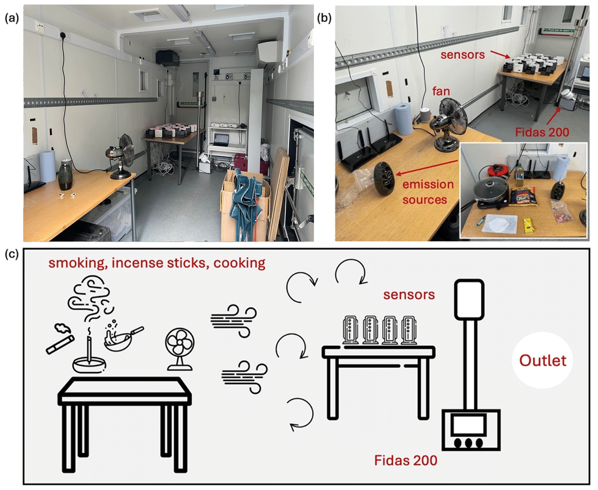
Figure 1 Overview of indoor air quality sensor calibration setup: (a) fully renovated half-size container, (b) emission sources and analytical instrumentation, and (c) schematic of pollutant generation and instrument placement.

2 Method

2.1 Experimental Configurations

A controlled laboratory experiment was conducted within a custom-built container designed to simulate realistic indoor air pollution conditions (Fig. 1a). The chamber was equipped with fans to ensure uniform pollutant distribution (Fig. 1b), which minimized spatial concentration variations, essential for maintaining stable and reproducible conditions during sensor evaluation. An aerosol spectrometer (i.e., Palas Fidas 200; detectable particle size of 0.18–18 µg, ranges from 0 to 10 000 µg m⁻³ with 9.7 % uncertainty for PM_2.5 measurements) was employed as the reference-grade instrument to provide high-precision baseline measurements for sensor performance evaluation and calibration. A total of 40 low-cost air quality sensors was deployed within the chamber, settled on a table at near the same height with Fidas 200 to minimize positional variability. Our air quality sensors consisted of two different types, including 20 units of AirGradient ONE (Model I-9PSL) and 20 units of AtmoCube. AirGradient ONE sensors measure PM_2.5 using a Plantower PMS5003 laser-scattering sensor (detectable particle size of 0.3–10 µg, with ± 10 µg m⁻³ at 0–100 µg m⁻³, ± 10 % at 100–500 µg m⁻³), and temperature and RH through a Sensirion SHT40 sensor. AtmoCube sensors detect particulate matter using a Sensirion SPS30 laser-scattering sensor (detectable particle size of 0.3–10 µg, with ± 5 µg m⁻³ at 0–100 µg m⁻³, ± 10 % at 100–1000 µg m⁻³), temperature using a Sensirion STS35-DIS, and RH using a Sensirion SHTC3.

To generate diverse and realistic indoor air pollution profiles, three indoor emission sources were introduced into the experimental container, including incense sticks, cigarette smoke from 7 to 21 October 2024, and cooking emissions (i.e., frying vegetables, bacon, and fries) from 22 to 30 October 2024 (Fig. 1b and c). All AirGradient ONE and AtmoCube sensors and the Fidas 200 were exposed to the same emission sources simultaneously. Temperature and RH levels were allowed to exchange passively with the outdoor air with no mechanical ventilation or windows/door opening, mimicking indoor conditions where these parameters may fluctuate. Between each emission event, the container was ventilated until pollutant concentrations returned to background levels (mainly during the night), ensuring that there was no cross-contamination between different test conditions, thus generating a reliable dataset for subsequent sensor performance evaluation and calibration (Qian and Dai, 2025).

2.2 Automated Machine Learning

We employed an AutoML framework to develop and select calibration models for the indoor air quality sensors (Qian and Dai, 2025). The AutoML approach generate a variety of (i.e., 30 in this study) candidate models and optimised their hyperparameters. Then the AutoML algorithm would identify a model that best maps the sensor outputs to the reference concentrations. In our implementation, the input features to each model included the sensor's raw readings, indoor temperature, and RH, while the target output was the PM concentration measured by Fidas 200.

This study used H₂O's splitFrame with a fixed seed (1014) to allocate 80 % of the rows to training and 20 % to a held-out test set. During AutoML, we used k-fold cross-validation (5-fold) on the training portion for model selection (sorted by root mean square error, RMSE). The held-out 20 % test set was never used for training or tuning; we report both cross-validated training metrics and external test metrics (see Table S1 in the Supplement). This choice ensured both train/test and cross-validation folds contained comparable concentration distributions while avoiding temporal leakage, as the experiment container was well-mixed and emission episodes were interleaved.

Evaluation metrics were calculated for each candidate to guide the selection of the best model. We primarily used the RMSE, normalized root mean square error (NRMSE), mean absolute error (MAE), symmetric mean absolute percentage error (sMAPE), mean bias error (MBE), index of agreement (IOA), and R² as the performance criteria. RMSE quantified the average magnitude of prediction errors in units matching the observed data, with lower values reflecting smaller deviations. We also use NRMSE to provide a dimensionless measure of error that allows model performance to be compared fairly across different concentrations. MAE measured the average absolute difference between observed and predicted values, providing an interpretable measure of accuracy independent of error direction. We also calculated sMAPE because it expresses errors as a bounded percentage relative to both observed and predicted values, making performance more comparable across different concentration ranges and less sensitive to extreme values. MBE provides the average bias in the predictions, where positive or negative values indicated overestimation or underestimation, respectively. IOA indicates the overall level of agreement (from −1 to 1) between reference measurements and predicted values, with 1 denoting perfect agreement (ideal model performance), 0 with no agreement (predictions no better than simply predicting the observed average), and −1 with complete disagreement or systematic inverse relationship (Willmott et al., 2011). R² (values in [0,1]) indicates the proportion of the variance in the reference measurements explained by the model, with values closer to 1 indicating a stronger linear association. The formulas are represented below:

$$\begin{array}{}\text{(1)}& {\displaystyle }\text{RMSE}=\sqrt{{\displaystyle \frac{\mathrm{1}}{n}}{\sum }_{i=\mathrm{1}}^n(o_i-p_i{)}^{\mathrm{2}}}\text{(2)}& {\displaystyle }\text{NRMSE}={\displaystyle \frac{\sqrt{\frac{\mathrm{1}}{n}{\sum }_{i=\mathrm{1}}^n(o_i-p_i{)}^{\mathrm{2}}}}{\stackrel{\mathrm{‾}}{o}}}\text{(3)}& {\displaystyle }\text{MAE}={\displaystyle \frac{\mathrm{1}}{n}}{\sum }_{i=\mathrm{1}}^n\left|o_i-p_i\right|\end{array}$$

$$\begin{array}{}\text{(4)}& {\displaystyle }\text{sMAPE}={\displaystyle \frac{\mathrm{100}}{n}}{\sum }_{i=\mathrm{1}}^n{\displaystyle \frac{\mathrm{2}\left|o_i-p_i\right|}{\left|o_i\right|+\left|p_i\right|}}\text{(5)}& {\displaystyle }\text{MBE}={\displaystyle \frac{\mathrm{1}}{n}}{\sum }_{i=\mathrm{1}}^n(o_i-p_i)\text{(6)}& {\displaystyle }\text{IOA}=\left\{\begin{array}{ll}\mathrm{1}-\frac{{\sum }_{i=\mathrm{1}}^n\left|p_i-o_i\right|}{c{\sum }_{i=\mathrm{1}}^n\left|o_i-\stackrel{\mathrm{‾}}{o}\right|},& \text{ when }{\sum }_{i=\mathrm{1}}^n\left|p_i-o_i\right|\\ & \le c{\sum }_{i=\mathrm{1}}^n\left|o_i-\stackrel{\mathrm{‾}}{o}\right|\\ \frac{c{\sum }_{i=\mathrm{1}}^n\left|o_i-\stackrel{\mathrm{‾}}{o}\right|}{{\sum }_{i=\mathrm{1}}^n\left|p_i-o_i\right|}-\mathrm{1},& \text{ when }{\sum }_{i=\mathrm{1}}^n\left|p_i-o_i\right|\\ & >c{\sum }_{i=\mathrm{1}}^n\left|o_i-\stackrel{\mathrm{‾}}{o}\right|\end{array}\right.\text{(7)}& {\displaystyle }{R}^{\mathrm{2}}=\mathrm{1}-{\displaystyle \frac{{\sum }_{i=\mathrm{1}}^n(o_i-p_i{)}^{\mathrm{2}}}{\sqrt{{\sum }_{i=\mathrm{1}}^n(o_i-\stackrel{\mathrm{‾}}{o}{)}^{\mathrm{2}}}}}\end{array}$$

here o_i denotes the ith value from the reference dataset, p_i is the ith predicted value from the calibration models, n represents the total number of data points in the dataset, and $\stackrel{\mathrm{‾}}{o}$ is the arithmetic average of all reference measurements.

After training the model, AutoML ranks candidates on its leaderboard by the RMSE obtained from k-fold cross-validation on the training set (Table S1). The highest-ranked model (Leader Rank 1) is therefore the model with the smallest cross-validated RMSE among all candidates. We adopt this criterion to (i) keep the 20 % test set independent of model selection (avoiding optimistic bias), (ii) obtain a more stable, lower-variance estimate by averaging errors across folds rather than relying on a single split, and (iii) prioritize a loss that penalizes large deviations, which is appropriate for PM_2.5 calibration (RMSE in µg m⁻³). After selection, all performance reported in the Results refers to the independent test set.

2.3 Calibration Procedure

To ensure reproducible calibration of the low-cost sensors against the Fidas 200, we first established a three-step protocol that accounts for variability among sensor units while maintaining consistency with reference measurements. The approach is designed to be scalable for large sensor networks in real-world indoor monitoring applications. The key steps include:

Field sensor-to-“Drift–reference sensor” calibration (f2d). A subset of five sensors from each sensor type (AtmoCube and AirGradient ONE) was randomly selected to serve as “drift–reference sensors”. These drift–reference sensors were used exclusively for calibration purposes and were not deployed for field indoor monitoring. The remaining sensors, referred to as “field sensors”, were intended for operational deployment. We employed AutoML to develop calibration models that map the field sensors' raw readings to the corresponding averaged measurements of the drift–reference sensors at each time step:

$$\begin{array}{}\text{(8)}& {\displaystyle }& {\displaystyle }\widehat{d_j}\left(t\right)=F_j^{f\mathrm{2}d}\left(x_j\right(t\left)\right)\text{(9)}& {\displaystyle }& {\displaystyle }{F}_j^{f\mathrm{2}d}=\arg {\sum }_{t=\mathrm{1}}^N{\left[f\left(x_j\right(t\left)\right)-\stackrel{\mathrm{‾}}{d}\left(t\right)\right]}^{\mathrm{2}}\text{(10)}& {\displaystyle }& {\displaystyle }{x}_j\left(t\right)={\left[s_j\left(t\right),T_j\left(t\right),{\text{RH}}_j\left(t\right)\right]}^{\mathrm{T}}\text{(11)}& {\displaystyle }& {\displaystyle }\stackrel{\mathrm{‾}}{d}\left(t\right)={\sum }_{k=\mathrm{1}}^K{d}_k\left(t\right)\end{array}$$

where $\widehat{d_j}\left(t\right)$ is calibrated PM concentration for field sensor j ($\mathrm{1},\mathrm{\dots },M$) at a time index of calibration record t ($\mathrm{1},\mathrm{\dots },N$); x_j(t) represents raw sensor reading, temperature, and RH; $\stackrel{\mathrm{‾}}{d}\left(t\right)$ denotes mean of K(=5) drift–reference sensors; and $F_j^{f\mathrm{2}d}$ represent best-performing model chosen for sensor j (GBM in this study) from pool of AutoML candidate models F during this f2d process. Note that here T_j(t) and RH_j(t) should be calibrated against averaged values of the drift–reference sensors using a simple univariate transfer function before being used as input features.

“Drift–reference sensor” to “Reference instrument” calibration (d2r). The averaged readings from drift–reference sensors were calibrated against Fidas 200 following similar procedure above:

$$\begin{array}{}\text{(12)}& {\displaystyle }& {\displaystyle }\widehat{r}\left(t\right)=F^{d\mathrm{2}r}\left(z\right(t\left)\right)\text{(13)}& {\displaystyle }& {\displaystyle }{F}^{d\mathrm{2}r}=\arg {\sum }_{t=\mathrm{1}}^N{\left[f\left(z\right(t\left)\right)-r\left(t\right)\right]}^{\mathrm{2}}\text{(14)}& {\displaystyle }& {\displaystyle }z\left(t\right)={\left[\stackrel{\mathrm{‾}}{d}\left(t\right),\stackrel{\mathrm{‾}}{T}\left(t\right),\stackrel{\mathrm{‾}}{\text{RH}}\left(t\right)\right]}^{\mathrm{T}}\end{array}$$

here $\widehat{r}\left(t\right)$ represents calibrated PM concentration for drift–reference sensors; r(t) is PM concentration measured by the reference instruments (Fidas 200); z(t) represents a vector of $\stackrel{\mathrm{‾}}{d}\left(t\right)$, and calibrated $\stackrel{\mathrm{‾}}{T}\left(t\right)$ and $\stackrel{\mathrm{‾}}{RH}\left(t\right)$ (against Fidas 200); and F^d2r denotes best-performing model for the d2r calibration.

Our exploratory analysis (Fig. S1 in the Supplement) revealed a clear threshold at 50 µg m⁻³ where the sensor bias flips. We chose this value because the scatter plot of sensor versus reference measurements shows two distinct regimes relative to the 1:1 line. At or below 50 µg m⁻³, the data cloud is tight and lies mostly above the 1:1 line, which indicates a positive sensor bias (overestimation) at low concentrations. Conversely, above 50 µg m⁻³ the cloud shifts below the 1:1 line, and the fitted trend becomes flatter than the 1:1 reference, a pattern consistent with signal compression and underestimation at higher particle loads. This split is further justified by the data distribution; most data lie below about 25 µg m⁻³, with only a small number of points between 25 and 100 µg m⁻³. A split at 50 µg m⁻³ produces two interpretable regimes that align with the observed change in bias, keeps the rare high-concentration events together, and avoids slicing the dense background data into very small groups, which would reduce model stability. Therefore, we applied a stratified calibration strategy, training separate AutoML models for the low (< 50 µg m⁻³) and high (50–600 µg m⁻³) regimes in both the field-to-drift (f2d) and drift-to-reference (d2r) stages. This allows us to tailor the calibration to the specific bias profile of each regime and thereby minimises systematic error across the sensor's full operating range.

Field sensor-to-“Reference instrument” calibration (f2r). For every time stamp t, the field sensor's raw reading is first converted to a drift–reference proxy as in Step (1) f2d. That proxy, combined with calibrated temperature and RH (against Fidas 200), is then fed into the calibration models in Step (2) d2r to calculate concentrations directly comparable to the reference dataset:

$$\begin{array}{}\text{(15)}& \stackrel{\mathrm{̃}}{r_j}\left(t\right)=H_j\left(x_j\right(t\left)\right)\equiv \left(F^{d\mathrm{2}r}\circ F_j^{f\mathrm{2}d}\right)\left(x_j\right(t\left)\right)\end{array}$$

where $\stackrel{\mathrm{̃}}{r_j}\left(t\right)$ denotes final PM concentration of sensor j aligned to Fidas 200; and H_j represents shorthand for the overall transfer function $F^{d\mathrm{2}r}\circ F_j^{f\mathrm{2}d}$.

The sensor performance drift over long deployments, the calibration derived pre-deployment gradually becomes less reliable. After retrieval we therefore rebuild the f2d and d2r models with the post-deployment dataset, obtaining a second set of predictions $\stackrel{\mathrm{̃}}{r_j^{\prime }}\left(t\right)$. For any timestamp t within the deployment period $\mathrm{0}\le t\le D$ (with D the total duration), we fuse the two predictions with a simple linear weight that shifts emphasis from the pre- to the post-deployment model:

$$\begin{array}{}\text{(16)}& r_j\times \left(t\right)=\left(\mathrm{1}-{\displaystyle \frac{t}{D}}\right)\times \stackrel{\mathrm{̃}}{r_j}\left(t\right)+{\displaystyle \frac{t}{D}}\times \stackrel{\mathrm{̃}}{r_j^{\prime }}\left(t\right)\end{array}$$

thus, r_j×(t) equals the pre-deployment estimate at the campaign start (t=0), the post-deployment estimate at the end (t=D), and a smoothly blended value in between, providing a first order correction for drift.

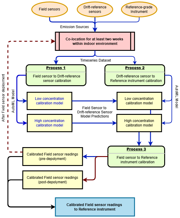
Figure 2 Flowchart of the indoor air quality sensor calibration strategy. The flowchart used a fixed colour scheme to distinguish the two stages of the workflow. Blue arrows and lines represent the main training and prediction path that spans Processes 1–3. The brown arrows and lines represent the post-deployment recalibration path, which is executed after sensor retrieval to correct drift using the post-deployment dataset. The resulting predictions are passed through Process 3 to obtain calibrated readings mapped to the reference instrument.

The overall calibration framework is shown schematically in Fig. 2.

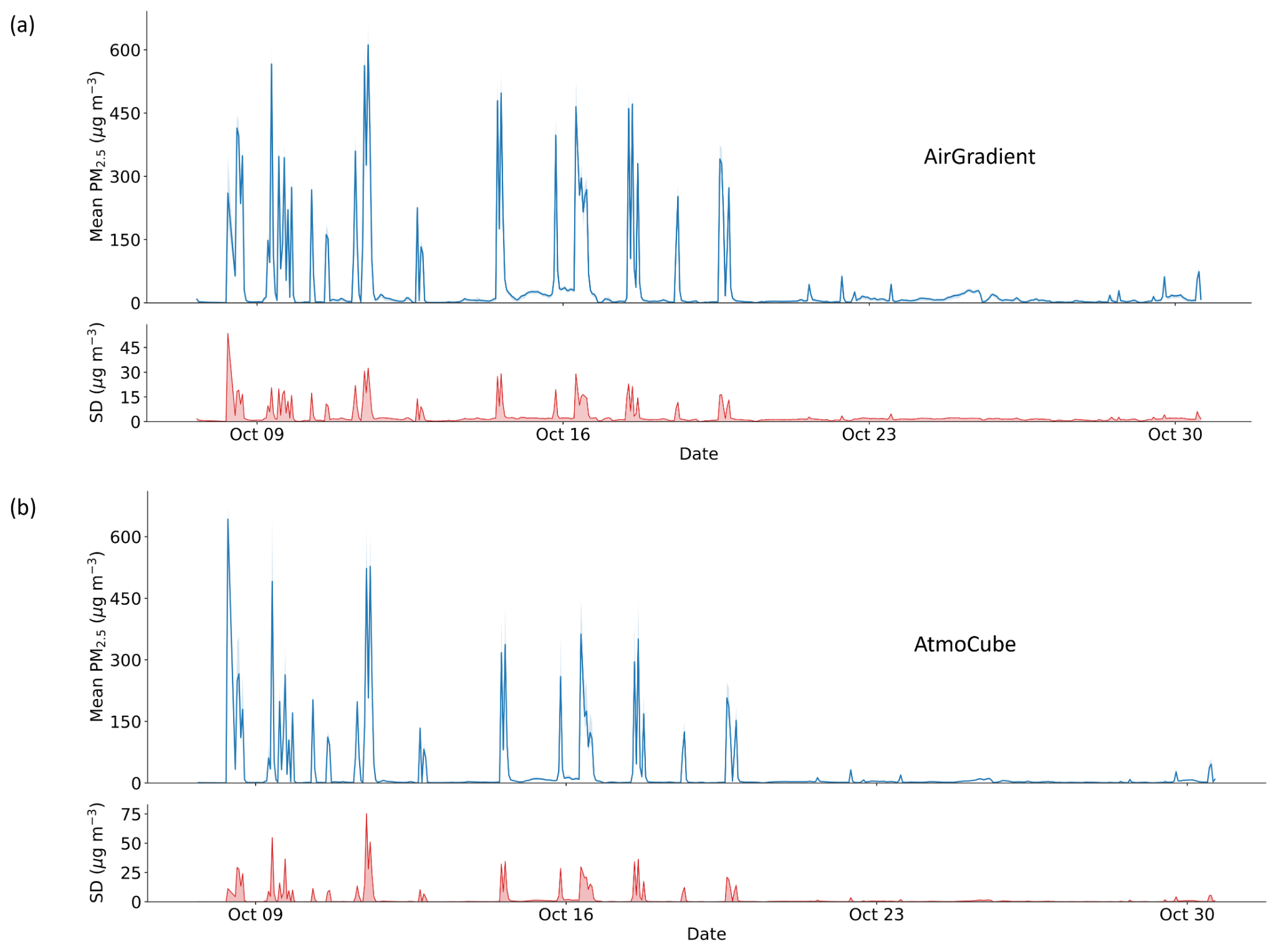
Figure 3 Timeseries of (a) Mean PM_2.5 readings from AirGradient ONE sensors and the standard deviations (SD) between them, (b) Mean PM_2.5 readings from AtmoCube sensors and the SD between them. The shaded areas represent the minimum to maximum values.

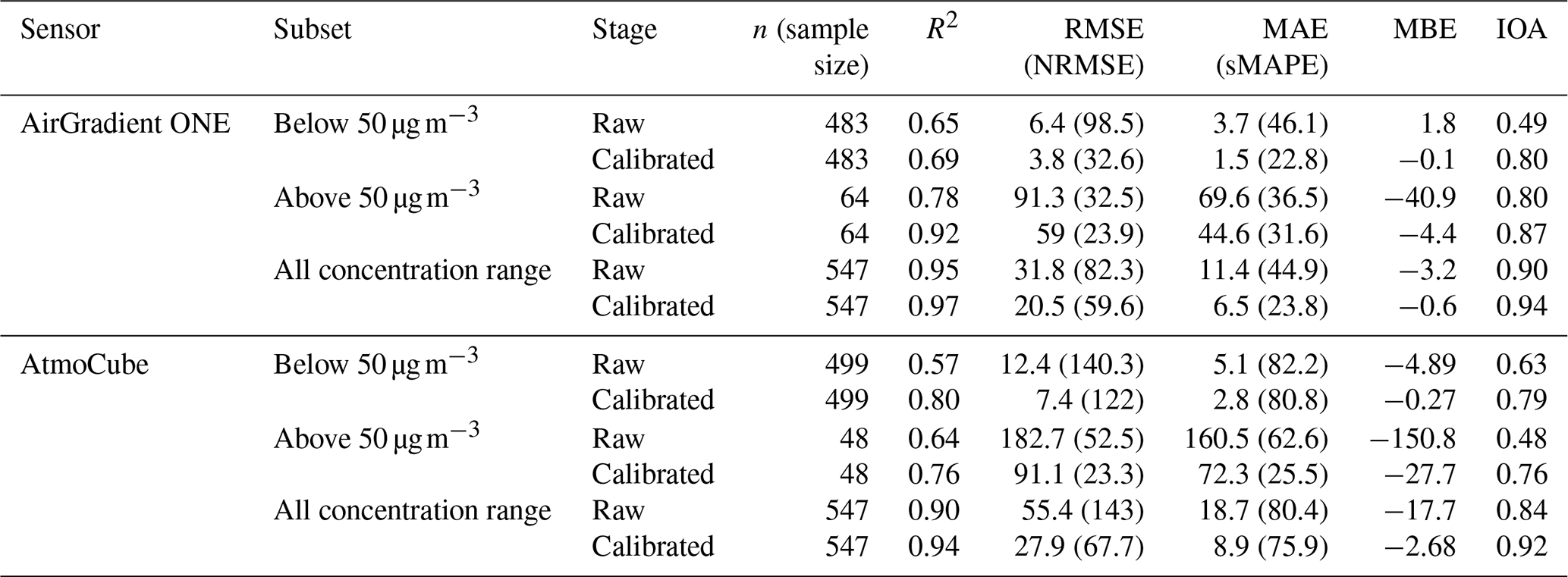
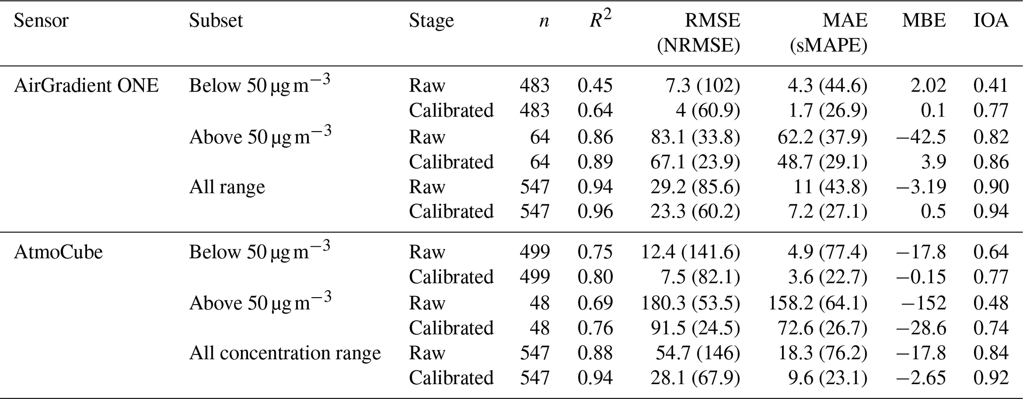
Table 1 Statistical performance of raw and calibrated AirGradient ONE and AtmoCube drift–reference sensors relative to the Fidas 200 measurements for PM_2.5, stratified by concentration regime (below-50, above-50) and for the combined dataset.

3 Results and Discussions

3.1 Low-cost sensor raw readings

Figure 3 compares the timeseries responses of the two sensor types, from AirGradient ONE and AtmoCube to indoor emission events. During the combustion episodes (cigarette smoking and incense-burning) that occurred between 12 and 22 October 2024, the AirGradient ONE sensors repeatedly recorded uncalibrated PM_2.5 concentrations exceeding 500 µg m⁻³, and all units tracked those peaks almost identically, showing high intra-sensor coherence and a high sensitivity to combustion-derived particles. The AtmoCube sensors followed the same temporal pattern but with systematically lower maximum concentrations compared to the AirGradient ONE sensors, with peak readings between 400 and 500 µg m⁻³. Cooking activities generated far lower PM concentrations. Routine meal preparation produced brief excursions of ∼ 30 µg m⁻³ on both sensor types, while a single spike of 80 µg m⁻³ on 30 October consistent with braise and fry high-fat foods that known to generate abundant aerosols (Xu et al., 2024). Therefore, although both AirGradient ONE and AtmoCube sensors correctly identified the timing of each emission episode, AirGradient ONE consistently reported higher absolute concentrations, particularly for the most intense combustion plumes than those of AtmoCube sensors.

The inter-type relationship is summarised in Fig. S2, showing the averaged drift-reference PM_2.5 measurements from AirGradient ONE and AtmoCube. At concentrations below 50 µg m⁻³ (hereafter denotes as “below-50”) (Fig. S2a), AirGradient ONE readings lay predominately above the 1:1 reference line, showing a positive bias relative to AtmoCube sensors. Once concentrations exceeded ∼ 50 µg m⁻³ (denotes as “above-50”) (Fig. S2b), this coherence vanished and the paired data became more scattered, indicating that the two sensor types diverge progressively with increasing particle load. Calibration that reconciles these type- (brand) specific sensitivities is therefore essential for any application that requires accurate absolute PM_2.5 values.

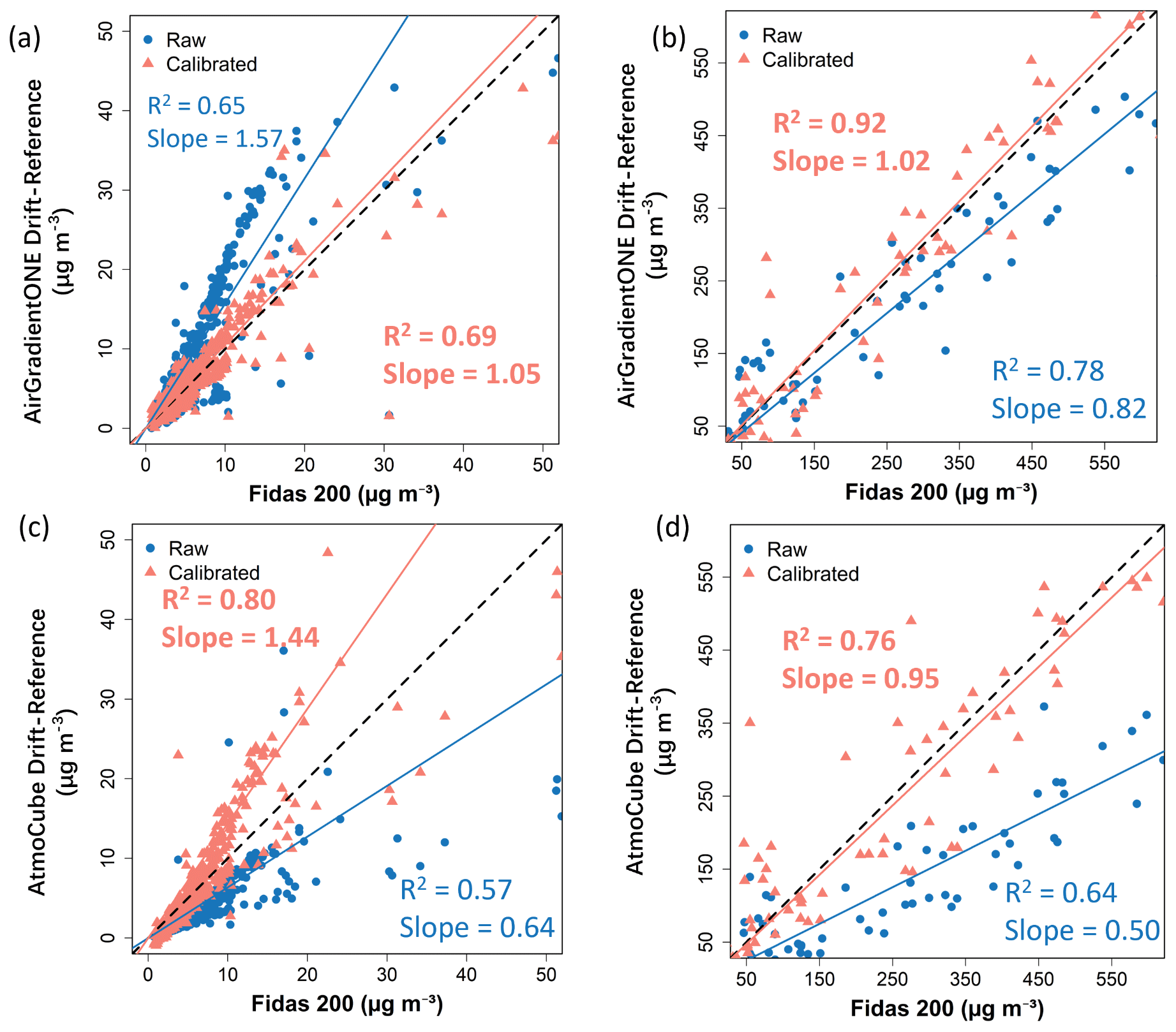
Figure 4 Raw and calibrated PM_2.5 of drift-reference sensors compared with the Fidas 200 measurements, (a) AirGradient ONE sensors within below-50 regime; (b) AirGradient ONE sensors within above-50 regime; (c) AtmoCube sensors within below-50 regime; (d) AtmoCube sensors within above-50 regime.

Sensor-measured environmental parameters exhibited similar systematic offsets (Fig. S3 for temperature and Fig. S4 for RH). Throughout the calibration, AirGradient ONE temperatures were 1.2–1.8 °C higher than those from AtmoCube (Fig. S3a and b), where paired data cluster above the identity line (slope = 1.01, R² = 0.94). AirGradient ONE measured 4 %–7 % lower than AtmoCube sensors for RH maxima, whereas at minima AirGradient ONE read 3 %–5 % higher, as in Fig. S4a and b. Intra-type variability reached ∼ 2 °C for AirGradient ONE sensors but was ≤ 1.5 °C for AtmoCube sensors, and both types recorded the same diurnal trend (Fig. S3c and d). RH measurements ranged from 47 % to 89 % (Fig. S4c for AirGradient ONE and Fig. 4d for AtmoCube). AirGradient ONE sensors exhibited tighter clustering (intra-type variability ≤ 5 %) than AtmoCube (≤ 10 %), but they showed a systematic pattern.

3.2 Raw readings from drift–reference sensors vs. Fidas 200 measurements

Figure 4a and c shows scatter plots of raw and calibrated averaged PM_2.5 concentrations from AirGradient ONE and AtmoCube drift-reference sensors against the Fidas 200 measurements in the below-50 regime, representative of relatively low air pollution. Before calibration, both AirGradient ONE and AtmoCube sensors exhibited moderate linear correlations with the Fidas 200, with R² values of 0.65 for the AirGradient ONE and 0.57 for the AtmoCube, respectively (Table 1). Although both sensor types clustered close to the 1:1 reference line, their slopes reveal systematic biases. AirGradient ONE readings lay predominately above the line with a regression slope of 1.57, producing an average 20 % overestimation relative to the Fidas 200, while AtmoCube readings fell below with a slope of 0.64, corresponding to a 55.6 % underestimation. Extending the analysis to the above-50 regime (Fig. 4b and d) highlights further divergence. Here, AirGradient ONE sensors had a stronger correlation with the reference (R² = 0.78), but its slope decreased to 0.82, reflecting a slight 3.1 % underestimation during high pollution episodes. In contrast, AtmoCube sensors had a lower slope of 0.50 and an R² of 0.64, showing a substantial 38.8 % underestimation. Therefore, both types of sensor experience signal compression at higher particle loads, yet the magnitude of this non-linearity is sensor specific.

RH can significantly influence the measurement accuracy of particles from indoor air quality sensors (Fig. S5). For AirGradient ONE (Fig. S5a and b), PM_2.5 readings above the 1:1 reference line at low concentrations consistently associated with periods of high RH, implying that hygroscopic growth of particles at high humidity is a primary driver of AirGradient ONE's low end overestimation (Liang, 2021). Conversely, AtmoCube showed no systematic RH pattern (Fig. S5c and d); its scatter remained broadly uniform across the humidity spectrum, indicating lower RH sensitivity. This disparity may reflect differences in internal RH-compensation algorithms implemented by each manufacturer.

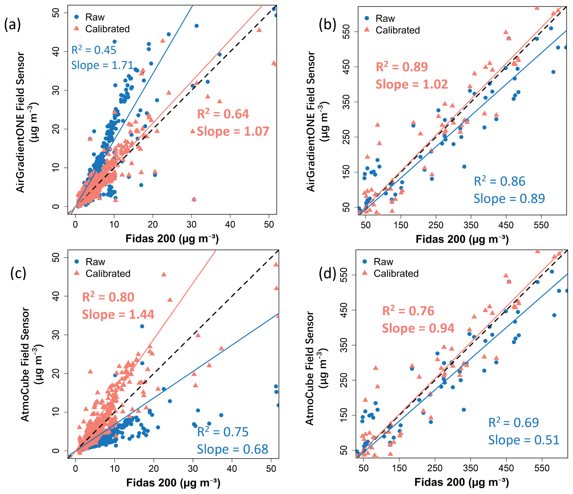
Figure 5 Raw and calibrated PM_2.5 of field sensors compared with the Fidas 200 measurements, (a) AirGradient ONE sensors within below-50 regime; (b) AirGradient ONE sensors within above-50 regime; (c) AtmoCube sensors within below-50 regime; (d) AtmoCube sensors within above-50 regime.

3.3 Calibrated readings from drift-reference sensor vs. Fidas 200 measurements

In the below-50 regime, calibrated AirGradient ONE drift-reference readings show slight stronger correlation with Fidas 200 measurements (R² = 0.69) compared to their raw values (Fig. 4a), and errors are relatively small and have been improved (NRMSE = 32.6 %, sMAPE = 22.8 %) as shown in Table 1. The residuals present negligible systematic bias (MBE = −0.1 µg m⁻³), indicating great improvements from systematic overestimation under low PM_2.5 concentration before calibration. After calibration, the sensor performance meets the recommended criteria of R² ≥ 0.70 and RMSE ≤ 7 µg m⁻³ (Zamora et al., 2022). At above-50 concentrations (Fig. 4b), the improvement in the performance of calibrated AirGradient ONE sensors was even more significant, with R² and IOA achieving about 0.92 and 0.87, respectively. The errors also have been improved (NRMSE = 23.9 %, sMAPE = 31.6 %) as expected and remain proportionally reasonable (e.g., ∼ 10 % uncertainty at 600 µg m⁻³). A slight negative bias (MBE  = −4.4 µg m⁻³) indicating a small underestimation tendency at extreme high concentrations, but high IOA value (0.87) show accurate tracking of both timing and magnitude.

Figure S6 show the impact of RH on calibrated readings of AirGradient ONE sensors for the below-50 (Fig. S6a) and the above-50 (Fig. S6b) concentration regimes, respectively. Across both concentration ranges the residuals show no systematic humidity bias, indicating that the AutoML model (using RH and temperature as covariates) mitigated hygroscopic growth influences that typically inflate optical counts above 70 %–80 % RH (Ko et al., 2024). The small scatter evident at extreme high RH levels likely reflects limited training data but does not compromise agreement with the reference, corroborating reports that RH-aware calibration can suppress sensor error by around 20 % (Liang, 2021).

Calibration likewise improved AtmoCube agreement with the Fidas 200 across the full concentration range (Fig. 4c and d). Overall AtmoCube sensors achieved R² = 0.94 and IOA = 0.92 (Table 1). In the below-50 clean air conditions, the calibrated AtmoCube sensors have R² = 0.80, and such slightly lower correlation relative to those of high pollution levels is expected as sensor signals approach the noise floor at very low pollution levels (Johnson et al., 2018). RMSE (7.4 µg m⁻³) and MAE (2.8 µg m⁻³) are relatively small, and the mean bias is negligible, indicating that the calibration mitigates the pronounced low-end under-reading observed pre-calibration. At high PM_2.5 levels, calibrated AtmoCube sensors still show good agreement with Fidas 200 as data points distribute along the 1:1 line but with slightly reduced R² (0.76). A possible explanation is that at very high particle loading the sensor's optical detector response starts to become non-linear or approaches a saturation point (Kelly et al., 2017), introducing larger random errors. The residual bias is minor (MBE = 27.7 µg m⁻³), indicating a small over-read under very high pollution. Figure S6c and d shows that, after calibration, AtmoCube residuals remain almost flat across the full RH ranges in both low and high concentration regimes. Even during episodes exceeding 80 % RH, no coherent over- or under-reading trend was found, indicating that the calibration has effectively reduced humidity interference.

Table 2 Statistical performance of raw and calibrated AirGradient ONE and AtmoCube field sensors relative to the Fidas 200 measurements for PM_2.5, stratified by concentration regime (below-50, above-50) and for the combined dataset.

3.4 Calibrated readings from field sensors vs. Fidas 200 measurements

The multi-stage calibration strategy effectively improved the performance of field sensors against the reference-grade instrument Fidas 200 (Fig. 5 and Table 2). Within the below-50 regime, AirGradient ONE sensors showed a RMSE of 4 µg m⁻³ and MAE of 1.70 µg m⁻³, and their correlation R² increased from 0.45 to 0.64. By contrast, AtmoCube sensors achieved a stronger linear match (R² = 0.80) despite relatively higher residual scatter (RMSE = 7.5 µg m⁻³) (Fig. 5c), consistent with their finer baseline sensitivity to subtle particulate variations. Performance at above-50 concentration regime indicated that both types of indoor air quality sensor synchronised well with the timing of pollution events while their error signatures differed. AirGradient ONE sensors showed moderate overestimation (MBE = 3.9 µg m⁻³, RMSE = 67.1 µg m⁻³, NRMSE = 23.9 %), while AtmoCube sensors displayed higher systematic bias (MBE = 28.6 µg m⁻³) and higher variability (RMSE = 91.5 µg m⁻³, NRMSE = 24.5 %). These differences may arise from different sensor components, for example, AtmoCube units employed shorter optical path length and proprietary firmware averaging while AirGradient ONE sensors used longer path and raw count reporting of the Plantower PMS5003. Importantly, our calibration strategy reconciled hardware-driven disparities between sensor types. Both types of sensors agreed well with Fidas 200 measurements after calibration, with IOA increasing from 0.90 to 0.94 for AirGradient ONE and from 0.84 to 0.92 for AtmoCube sensors.

To evaluate the multi-step calibration strategy itself rather than the choice of models, we compared AutoML models with multivariate regressions (Fig. S7). Figures S7 and S8 show that AutoML models produced better performance statistics, showing enhanced predictive accuracy and reliability, particularly when evaluating error distribution across different PM_2.5 concentration regimes. Such improvements could be due to the ability of AutoML to incorporate interaction terms (RH, temperature) that influence the sensor light-scattering response (Liang, 2021). However, there is only one exception for AtmoCube sensors in the over 100 µg m⁻³, in which the linear model has a smaller sMAPE. This is might due to the limited amount of data in the high concentration range.

3.5 Limitations and implications

Our framework significantly improved the low-cost sensors performance under different concentrations. But there are still some limitations, and further research is needed on the generalizability of the model and calibration strategies. Firstly, the training data were collected in a single experimental container under temperate-climate humidity (with RH between 45 %–85 %) and may not capture sensor behaviour in very moist interiors. Secondly, the present study did not capture every indoor emission source, particularly those with moderate emission levels. We do not know whether the sensors will be sensitive to particle types (e.g., particles from different sources). Furthermore, evaluating sensor drift demands the months-to-years timescales of real deployments and was not evaluated. Future work should gather data from warmer, high-humidity homes to capture sensor behaviour at elevated RH conditions, consider additional moderate emission sources such as off-gassing materials, and run multi-year field trials to quantify drift and test automated recalibration. These steps will increase the robustness and evaluate long-term accuracy of the calibration strategy. However, the thresholds delineating “low” and “high” categories are derived from empirical observations within the analysed dataset. Accordingly, researchers are encouraged to initially assess their own data and adapt this strategy as necessary to ensure its applicability. In our case, there were limited data of high concentration, future studies should generate more emission to have more high concentration data to capture the full range performance.

The implications of our findings are significant for atmospheric science and indoor air quality management, especially in the context of the growing use of low-cost sensors for exposure assessment and public health applications. By showing that inexpensive sensors can be calibrated to yield high-quality data indoors, this study helps bridge the important gap between indoor and outdoor air pollution monitoring. Furthermore, the application of AutoML in sensor calibration showcases the value of advanced data-driven techniques in atmospheric measurements. AutoML could be used to periodically re-calibrate hundreds of sensors automatically as new reference data become available, maintaining network accuracy with minimal human intervention. This is particularly relevant for community science projects or indoor air quality campaigns where resources for manual calibration are limited. By improving the reliability of indoor air measurements, the study contributes to a future where continuous indoor air quality monitoring is feasible on a large scale, driving better-informed strategies to safeguard public health in the spaces where people live and work.

The regime thresholds used in this study were derived empirically from our indoor dataset and should not be assumed for other indoor cases, outdoors, or for other pollutants. Users should re-estimate cut points from their own co-located data and retrain the staged models with environment appropriate features.

4 Summary

In this work, we introduced an automated machine learning (AutoML) calibration framework for enhancing the performance of low-cost indoor air quality sensors. The AutoML-calibrated sensors met or exceeded study objectives by significantly improving measurement accuracy for fine particles (PM_2.5) across all concentration regimes. The multi-stage calibration workflow achieved tight agreement with reference measurements (from Fidas 200), evidenced by substantial increases in coefficient of determination (R²) and reductions in error metrics. In the low-concentration regime (below 50 µg m⁻³), R² improved from moderate values (∼ 0.6 pre-calibration) to approximately 0.85 post-calibration, with root-mean-square error (RMSE) dropping by roughly half (e.g., from ∼ 5 to ∼ 3 µg m⁻³), as well as the NRMSE. At higher concentrations (above 50 µg m⁻³), gains were even more pronounced, with R² approaching or exceeding 0.90 (near reference-grade performance) and RMSE falling from tens of µg m⁻³ to single digits. Similarly, mean absolute error (MAE) and symmetric mean absolute percentage error (sMAPE) declined markedly, and mean bias error (MBE) was effectively eliminated, shifting from significant systematic biases (e.g., 5–10 µg m⁻³ over- or underestimation) to nearly zero. These results show that the calibrated sensors reliably resolve indoor particulate levels at background concentrations and during elevated pollution events, closely tracking the reference instrument across the full range. These findings confirm that our multistage calibration effectively eliminated sensor bias under varied indoor conditions and emission sources. The initial stage corrected baseline drift. Subsequent stages used AutoML to address scatter caused by relative humidity and nonlinear responses at high particle concentrations. These factors are often overlooked in simpler methods. AutoML efficiently selected the best models for each phase, removed the need for manual tuning, and revealed subtle patterns in the data. By integrating AutoML into a structured multistage process, we achieved robust bias correction across scenarios, yielding accurate, precise measurements well-suited for indoor air quality monitoring.