Spectral versus co-spectral correction of eddy-covariance fluxes: a multi-site assessment across the ICOS network

Accurate correction of high-frequency attenuation remains a critical challenge in eddy-covariance measurements of turbulent gas fluxes. Experimental correction approaches based on either power spectra or co-spectra are widely used, yet their relative behaviour and implications for flux estimates have not been systematically assessed across sites and atmospheric conditions.

This study presents a multi-site comparison of these two approaches using one year of CO₂ and H₂O flux data from 38 ecosystem stations of the Integrated Carbon Observation System (ICOS) equipped with a standardized enclosed-path gas analyser setup. To support reproducibility and facilitate future methodological intercomparisons, we additionally provide an open-source and configurable software tool implementing both correction approaches.

Overall, the ICOS setup exhibited limited high-frequency attenuation, with correction factors generally below 1.2 for CO₂ and occasionally approaching 2 for H₂O under humid conditions. For CO₂, differences between methods remained small after standard turbulence filtering, with cumulative flux differences typically below 2 %. In contrast, H₂O corrections showed larger discrepancies, frequently reaching 5 %–10 % on cumulative fluxes. The largest differences occurred under stable atmospheric conditions, at low measurement heights, and under strong attenuation. Results indicate that CO₂ attenuation is dominated by sensor-separation effects, whereas H₂O attenuation is primarily controlled by adsorption–desorption processes within the sampling system.

The comparison highlights methodological limitations of both approaches. Both methods rely on assumptions regarding spectral similarity, but departures from these assumptions were found to affect gas spectra much more strongly than co-spectra, particularly for H₂O under humid conditions. In addition, spectral corrections were frequently affected by high-frequency noise and required dedicated denoising procedures, while sensor-separation effects had to be introduced through analytical formulations. Overall, the co-spectral approach provided more robust and physically consistent results across sites and atmospheric conditions.

A comparison with fluxes produced by the ICOS Ecosystem Thematic Centre revealed systematic differences that were often larger than those observed between the spectral and co-spectral approaches themselves, especially for H₂O. These results demonstrate the effectiveness of setup standardisation across the ICOS network while identifying high-frequency attenuation correction as a remaining source of uncertainty. They also highlight the need for a broader reassessment of this processing step within the ICOS flux-processing pipeline.

1 Introduction

The eddy-covariance (EC) method is the standard micro-meteorological technique to measure energy, momentum and gas turbulent exchanges between the land surface and the atmosphere. By measuring gas concentrations and wind components at high frequency (typically 10–20 Hz), it allows a direct and non-invasive estimation of fluxes at the ecosystem-parcel scale (Aubinet et al., 2012; Baldocchi, 2014). Despite its widespread application and the continuous technological advances improving the reliability of the instruments, the EC method is still bound to some technical limitations. One major and well-known source of bias is the correction of spectral attenuation of the measured signal, which, if not correctly accounted for, causes a systematic underestimation of the fluxes. Commonly analysed in the frequency domain, attenuation can affect both low- and high-frequency end of the signal spectrum (Moore, 1986; Aubinet et al., 2000; Massman, 2000; Massman and Clement, 2005). Signal loss in the high frequencies (low-pass attenuation) results from the physical characteristics of the sampling system like limited sampling time, line averaging, sensor separation and, for (en)closed-path gas analysers, air sampling through tubes and filters. Depending on the setup, the site characteristics, and atmospheric conditions, it can range from a few percent to several tens of percent of the actual flux, and a reliable quantification and correction of this attenuation is a major issue for the flux community (Massman and Clement, 2005).

Careful instrumentation and mounting set-up choices can reduce signal losses. This is the case with the enclosed-path ${\mathrm{CO}}_{\mathrm{2}}/{\mathrm{H}}_{\mathrm{2}}\mathrm{O}$ gas analyser from LI-COR Biosciences Inc. (Lincoln, NE, USA), which has been designed to combine the benefits of open-path and closed-path analysers so that, thanks to its compact size, it can be deployed with a short intake tube (typically < 1 m), thus reducing losses due to damping of fluctuations in the air sampling tube. This type of instrument is dictated within certain flux tower networks, such as the European ICOS network (Integrated Carbon Observation System, Franz et al., 2018) and the American NEON network (National Ecological Observatory Network, https://www.neonscience.org, last access: 20 September 2026). Despite these efforts, spectral corrections are still needed.

Multiple methods have been developed to quantify and correct the low-pass filtering effect of EC systems. They are commonly categorised as analytical (based on theoretical considerations) or experimental (based on in situ measurements) (Massman and Clement, 2005). Both approaches aim at describing the EC filtering effect through a transfer function (Moore, 1986), and the flux attenuation through its application to an unattenuated co-spectrum. The analytical method defines the total transfer function as a convolution of individual transfer functions describing each cause of attenuation individually (Moore, 1986; Moncrieff et al., 1997; Massman, 2000), and is commonly used for anemometer or open-path gas analyser fluxes (Massman and Clement, 2005). Recognition of other sources of spectral losses in more complex EC systems, such as the presence of particle filter(s) and rain caps in the gas sampling system, is necessary. The same applies to the non-neutral spectral characteristics of some gases in (en)closed-path analysers, which are associated with the adsorption and desorption of water molecules in the tube and influenced by air relative humidity. For these sources of flux loss, either no transfer function expressions are available, or the relevant transfer functions depend on aspects that are difficult to parameterise, such as the evolution of tube dirtiness. In all these cases, an experimental approach is recommended (Ibrom et al., 2007; Mammarella et al., 2009). In this approach, the transfer function is computed as the ratio of either power spectra or co-spectra of target gas concentration to sonic temperature. The sonic temperature is assumed to be the unattenuated reference, and thus the sensible heat co-spectrum is used for the correction factor estimation (Aubinet et al., 2000).

The use of power concentration spectra or co-spectra of concentration and vertical wind speed is an important and debated choice. Various studies support the use of power concentration spectra (Ibrom et al., 2007; Fratini et al., 2012; Nemitz et al., 2018). The main arguments are that the inclusion of the vertical wind speed signal does not add any relevant information on the gas spectral attenuation and introduces the need to additionally account for a phase shift which is generally difficult to determine (Ibrom et al., 2007). The power spectra approach is used in the popular EddyPro software package (LI-COR Biosciences, Lincoln, NE, USA), and recommended and applied in the ICOS methodology (Sabbatini et al., 2018). However, others defend the use of co-spectra (Aubinet et al., 2000; Mammarella et al., 2009, 2016; Wintjen et al., 2020), mainly because they are not affected by high-frequency noise and do not require an additional correction term for sensor separation.

While site-, gas- or instrument-specific studies have been performed to assess the best spectral correction procedure and options (Wintjen et al., 2020; Peltola et al., 2021; Aslan et al., 2021; Smidt et al., 2025; Reitz et al., 2022), no systematic comparison of spectral vs. co-spectral approach has been done so far.

In this study we propose a multi-site, data-driven comparison among spectral and co-spectral correction approaches. We based our analysis on the experimental setup adopted in the ICOS network at Class 1 and Class 2 ecosystem stations. We (i) highlight the conditions in which the methods diverge; (ii) quantify and (iii) assess the differences, (iv) highlight the best practices. By doing so, we also give an overall picture of the importance of high-frequency losses for the ICOS EC setup and of the effectiveness of the setup standardisation. Finally, we compare our spectral corrections to the one implemented within the ICOS processing pipeline delivering flux products widely used by the community.

2 Materials and methods

2.1 Sites and datasets

The data used in this study came from 38 ICOS Class 1 and 2 stations measuring CO₂ and H₂O fluxes (Table F1). The analysis was based on the 2024 data, the latest dataset available when most of the analyses for this paper were performed. The EC setup is standard at all ICOS sites and it is composed of a LI-7200(RS) (LI-COR Biosciences Inc., Lincoln, NE, USA) infrared gas analyser (IRGA) and one Gill HS-50 or HS-100 (Gill Instruments Ltd., Lymington, UK) 3-D sonic anemometer (Rebmann et al., 2018). All sites were equipped with a standard LI-COR heated 0.73 m-long sampling line of 5.33 mm of inner diameter, a LI-COR rain cap and a 2 µm inlet filter (Swagelok Company, Solon, OH, USA). The flow rate was fixed at each site, at a value between 10 and 16 L min⁻¹ according to site specifications. The only exception was FR-Gri that switched several times between 12 and 15 L min⁻¹ until the end of April, after which the flow rate was fixed at 12 L min⁻¹. The acquisition rate was 20 Hz for 29 sites and 10 Hz for the remaining 9. According to ICOS instructions (Sabbatini and Papale, 2017), the horizontal and vertical distances between the center of the anemometer sensing volume and the center of the sphere that encloses the IRGA raincap should be in the range $\mathrm{23.5}/\mathrm{31}$ and $\mathrm{0}/-\mathrm{0.05}$ cm, respectively. In practice, few exceptions to this rule are encountered (Fig. 1).

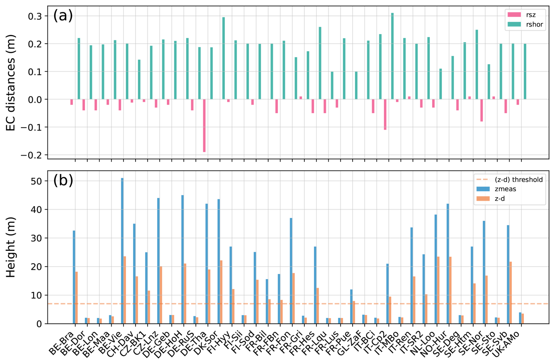
Figure 1 Overview of sites' principal metadata. Panel (a) shows the distances between the IRGA and the SA. The vertical separations (rsz in purple) indicate whether the inlet of the IRGA was above (positive) or below (negative) the centre of the sampling path of the SA. Measurement height and height above zero-plane (z−d) are displayed in panel (b). The dashed line denotes the z−d threshold to define high- and low-measurement-height sites, above and below it, respectively.

The measurement heights across the 38 sites varied over a wide range, reflecting the diversity of ecosystems measured, from peatlands and shrublands to croplands and grasslands, and up to forests (Fig. 1 and Table F1). Stations were classified into two categories, according to their height above the displacement plane (z−d). After visual inspection of z−d values and cross-checking with the characterisation of the ecosystem type, a clear distinction emerged between forests, with z−d above 7 m, and other ecosystems, where z−d was below 7 m (maximum 4 m). Those two categories were defined as high- and low-measurement-height sites, respectively (HMH and LMH).

The half-hourly fluxes uncorrected for frequency losses, data quality tests, as well as binned spectra and co-spectra used throughout this study, were computed by the ICOS Ecosystem Thematic Center (ETC), through the standard ICOS pipeline (Sabbatini et al., 2018; Vitale et al., 2020), using EddyPro (version 7.0.9), leading to the 2025 archive product (ICOS RI et al., 2025). To compute the fluxes, the following main processing steps were performed: block average to compute the fluctuations around the mean and covariance maximisation to correct for time-lag. Spectra and co-spectra were computed for each half-hour using the Fourier transform and smoothed using fifty exponentially spaced frequency bins.

The frequency losses were corrected for using either our own implementation, described in the following section, or the standard ICOS pipeline that relies on correction of high-pass attenuations according to Moncrieff et al. (2004) and correction for low-pass attenuations according to Fratini et al. (2012), including cross-wind and vertical sensor separation by Horst and Lenschow (2009) and correction for the anemometer path averaging and time response (Moore, 1986).

2.2 Spectral analysis and correction

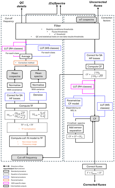
The general principles of an experimental spectral correction procedure are presented in Fig. 2. They are generally well established, and follow for both spectral and co-spectral approaches the same steps. The main gas- and method-specific options and parametrizations, which are user-defined, are also highlighted (orange, blue and magenta elements in Fig. 2).

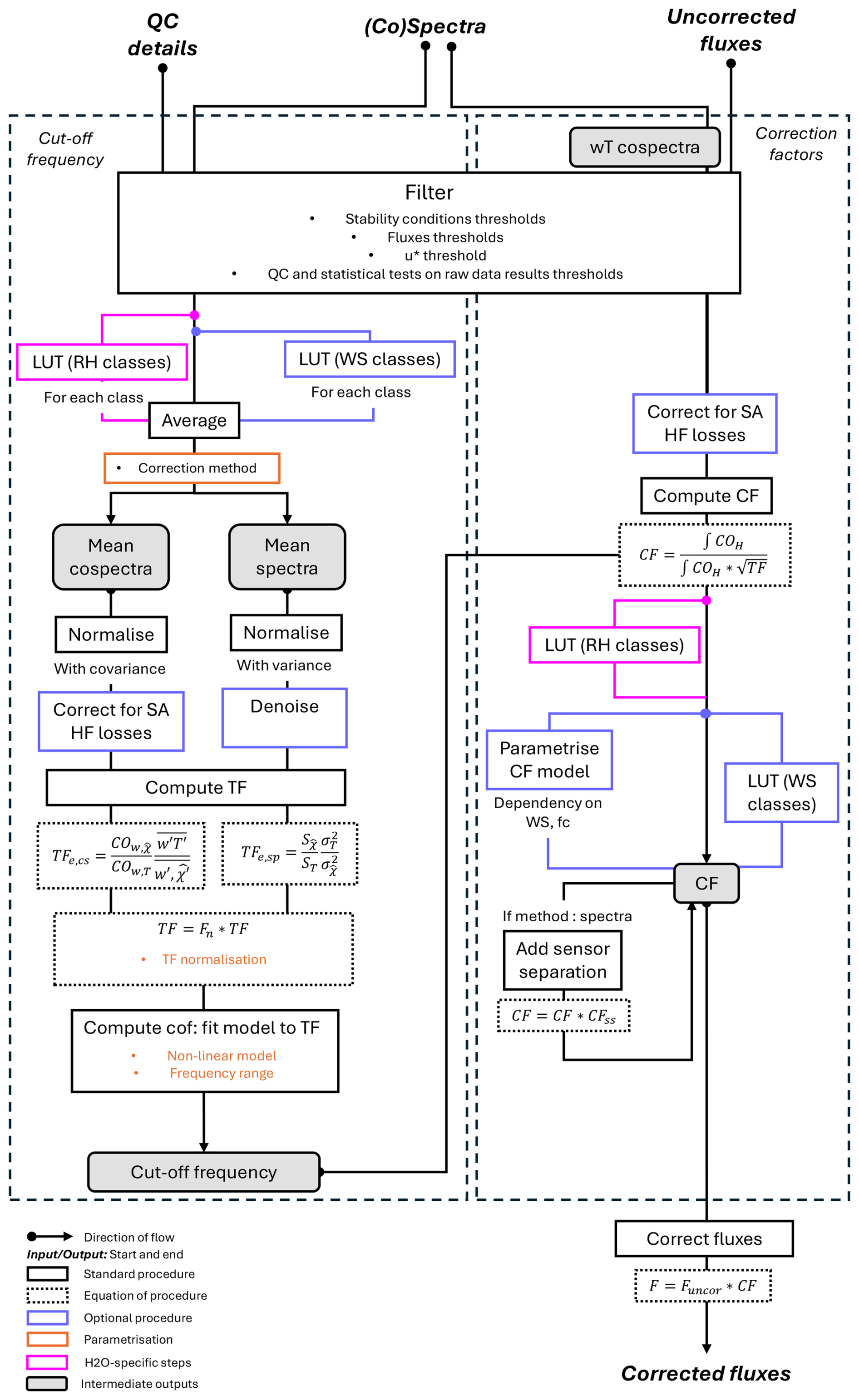
Figure 2 Flowchart of an experimental spectral correction procedure. On the left side, the general procedure to compute the system cut-off frequency. On the right side, the computation of correction factors to be applied to half-hourly data to obtain spectrally-corrected fluxes. For both parts, in addition to the main branch, details on potentially impactful parametrisation options (orange), optional procedures (blue), and gas-specific dependencies (H₂O on relative humidity, magenta) are presented. LUT stands for “look-up table” and other acronyms are introduced in the main text.

Only high-frequency spectral losses were considered here. The analysis was performed in the frequency domain, using the (co-)spectra to assess the high-frequency attenuation and compute the flux correction factors. The approach used in this work relied on the use of meteorological data classes and average values. Based on the theorised dependencies found in the literature (Moore, 1986; Moncrieff et al., 1997; Aubinet et al., 2000), wind speed classes were used for both gases and computation steps, namely cut-off frequency (cof) and correction factor (CF) estimation. For H₂O only, an additional classification based on relative humidity (RH) was applied, as spectral attenuations of water fluxes have been shown to be driven by the adsorption and desorption processes of water molecules in the sampling tube of the IRGA that varies with RH (Ibrom et al., 2007; Mammarella et al., 2009). Finally, for the specific purpose of investigating the theorised dependence of sensor separation CFs to wind direction (Horst and Lenschow, 2009) and for CO₂ only, an additional assessment by wind direction classes was performed. In all three cases, a fixed number of classes containing an equal number of data points was used.

As an initial filtering step common to both cut-off frequency and correction factor computations, only data for which wind speed (WS), wind direction (WD), dimensionless stability parameter ($\frac{z}{L}$), sensible heat flux (H), tracer flux (CO₂ or H₂O accordingly) and, for H₂O only, RH were available were retained. In addition, considering the horizontal geometry of the sonic anemometer used in ICOS, an additional site-specific wind direction filter was applied to remove data affected by flow distortion caused by the horizontal boom supporting the sonic transducers.

2.2.1 Cut-off frequency computation

The EC system signal attenuation in the high frequency range can be described with a first-order low-pass filter (Horst, 1997; Eugster and Senn, 1995). This transfer function (TF) can be estimated empirically from the ratio of the attenuated to ideal (co-)spectra. Assuming spectral similarity (Ohtaki, 1985), the equations can be written as:

$$\begin{array}{}\text{(1)}& {\displaystyle }{\text{TF}}_{\text{cs}}=F_{\mathrm{n}}{\displaystyle \frac{{\text{CO}}_{\mathrm{w},\widehat{\mathit{\chi }}}}{{\text{CO}}_{\mathrm{w},\mathrm{T}}}}{\displaystyle \frac{\stackrel{\mathrm{‾}}{w^{\prime }{T}^{\prime }}}{\stackrel{\mathrm{‾}}{w^{\prime }{\widehat{\mathit{\chi }}}^{\prime }}}}\text{(2)}& {\displaystyle }{\text{TF}}_{\text{ps}}=F_{\mathrm{n}}{\displaystyle \frac{S_{\widehat{\mathit{\chi }}}}{S_{\mathrm{T}}}}{\displaystyle \frac{{\mathit{\sigma }}_{\mathrm{T}}^{\mathrm{2}}}{{\mathit{\sigma }}_{\widehat{\mathit{\chi }}}^{\mathrm{2}}}}\end{array}$$

where CO_w,T and S_T are, respectively, the sensible heat co-spectra and sonic temperature spectra, considered as ideal (not affected by attenuation), and CO${}_{\mathrm{w},\widehat{\mathit{\chi }}}$ and $S_{\widehat{\mathit{\chi }}}$ the attenuated (co-)spectrum. Both spectra and co-spectra are normalised by their respective (co)variance (${\mathit{\sigma }}_{\mathrm{T}}^{\mathrm{2}}$, ${\mathit{\sigma }}_{\widehat{\mathit{\chi }}}^{\mathrm{2}}$, $\stackrel{\mathrm{‾}}{w^{\prime }{T}^{\prime }}$, $\stackrel{\mathrm{‾}}{w^{\prime }{\widehat{\mathit{\chi }}}^{\prime }}$). As these might also be affected by high-frequency losses, an additional normalisation factor (F_n) is included to ensure spectral similarity (Ibrom et al., 2007).

In order to establish the TFs and relative cofs describing each system, only best-quality (co-)spectra were selected, filtering for fluxes and quality flag thresholds as reported in Table 1. Then, normalized (co-)spectra above a plausibility threshold of 250 were discarded. A final outlier screening discarded any half-hour (co-)spectrum for which, within the 0.005–0.1 Hz band, at least 15 % of frequency bins lay outside pointwise log10-based IQR bounds ($Q\mathrm{1}-\mathrm{2.5}\times \text{IQR}$, $Q\mathrm{3}+\mathrm{2.5}\times \text{IQR}$) computed across the ensemble.

The filtered (co-)spectra were split into constant-size classes of WS, and RH for H₂O only. The WS classification accounts for a possible dependence of the cof on WS, which arises from the sensor separation term (Moore, 1986). In theory, this effect should appear only in the co-spectral approach, since it integrates all attenuation sources into the cof. In contrast, the spectral approach applies the sensor separation effect later, at the CF level (see Sect. 2.2.2). The RH classification accounts for the known dependence of cof on air humidity in the sampling tube and filters, which arises from the adsorption–desorption of water molecules on surfaces (Ibrom et al., 2007). At this point, a quality check was performed, so that if less than 2 (co-)spectra per class were present, the procedure was stopped.

Then, (co-)spectra in each class were averaged, resulting in one ideal and one attenuated (co-)spectrum per class. At this stage, only for the spectral approach was the presence of high-frequency noise in the mean real spectra assessed. When present, noise was removed using the procedure developed by Aslan et al. (2021), and a noise-free version of the spectra was produced. The details of the denoising procedure are reported in Appendix A, including some modifications to the original one which showed limitations in multi-site applications.

Next, the empirical TF was computed for each class as the ratio of real to ideal normalised (co-)spectra averages (Eqs. 1 and 2). The spread of the data in the frequency range at which no attenuation occurred, where the ratio was expected to result in a plateau, was checked. After preliminary analysis and visual inspection, the plateau check range was set at 0.021–0.34 Hz. If the coefficient of variation of the data exceeded 1, the TF of that class was discarded for poor quality.

A Lorentzian equation was fitted to the valid experimental TFs. For co-spectral TFs, the Lorentzian was modified according to Peltola et al. (2021) (P21 hereafter), to account for the impact of the phase shift induced by the time-lag covariance maximisation correction on the data:

$$\begin{array}{}\text{(3)}& {\displaystyle }{\text{TF}}_{\text{ps}}=F_{\mathrm{n}}{\displaystyle \frac{\mathrm{1}}{\mathrm{1}+{\left(\frac{f}{f_{\mathrm{c}}}\right)}^{\mathrm{2}}}}\text{(4)}& {\displaystyle }{\text{TF}}_{\text{cs(P21)}}\approx F_{\mathrm{n}}\sqrt{{\displaystyle \frac{\mathrm{1}}{\mathrm{1}+{\left(\frac{f}{f_{\mathrm{c}}}\right)}^{\mathrm{2}}}}}\end{array}$$

Equations (3) and (4) define the two functions, where ps stands for power spectra, cs for co-spectra, F_n is the additional normalisation factor, f [Hz] represents the natural frequency and f_c [Hz] the characteristic frequency parameter.

For the classic Lorentzian approach (Eq. 3), the cof corresponds to the half-power frequency, at which the TF equals 0.5. In the modified Lorentzian formulation of Peltola (Eq. 4), the TF equals $\frac{\mathrm{1}}{\sqrt{\mathrm{2}}}$ at f=f_c, and therefore the half-power cut-off frequency is reached at $f=\sqrt{\mathrm{3}}{f}_{\mathrm{c}}$. Nevertheless, the notation f_c and the acronym cof were retained for consistency with Eq. (3) and with the subsequent CF computations. Because of these different definitions, direct comparison of the fitted f_c parameters was not possible, and the corresponding half-power cut-off frequency was additionally computed and shown for the co-spectral approach, although it was not used for the computation of CFs.

Equation (4), while being only an approximation of the true transfer function, was considered (fortuitously) approximately correct in the relevant frequency range by Peltola et al. (2021), diverging from the true TF only under very strong attenuation.

The fitting range, chosen after some preliminary analysis and visual inspection, was set for all cases between 0.021 and 10 Hz. This procedure resulted in one cof per WS (and RH) class.

2.2.2 Correction factor computation and fluxes correction

The correction factors (CFs) can be computed as the ratio of the unattenuated and the measured flux. Using the properties of co-spectra integrals, and assuming spectral similarity, this can be written as:

$$\begin{array}{}\text{(5)}& \text{CF}={\displaystyle \frac{{\int }_{f_{min}}^{f_{max}}{\text{CO}}_{\mathrm{w},\mathrm{T}}\left(f\right)\mathrm{d}f}{{\int }_{f_{min}}^{f_{max}}{\text{CO}}_{\mathrm{w},\mathrm{T}}\left(f\right)\sqrt{\text{TF}\left(f_{\mathrm{c}}\right)}\mathrm{d}f}}\end{array}$$

where CO_w,T is the sensible heat co-spectrum (ideal), TF is the system transfer function as defined in Eqs. (3) or (4) and their product the attenuated co-spectrum. The lower (f_min) and upper (f_max) integration limits are determined by the flux averaging interval and half the acquisition frequency (Nyquist frequency), respectively. The use of the square root for the TF is according to Fratini et al. (2012) for the spectral approach, and Peltola et al. (2021) for the co-spectral approach.

The computation was performed separately for unstable ($\frac{z}{L}$ < 0) and stable ($\frac{z}{L}$ > 0) conditions, to account for differences in the position and shape of the reference co-spectra according to the stability regime (Kaimal et al., 1972). First, only good-quality sensible heat co-spectra were selected. Filtering was based on H flux value and the quality flags, with different thresholds depending on the stability regime, as reported in Table 1. For each remaining half-hour, a CF was computed. In order to do so, the TF was first constructed with the cof corresponding to the (RH and) WS of the given half-hour. The CF was then computed according to Eq. (5) for each valid averaging period.

The full series of half-hourly CF was sorted into (RH and) WS constant-size classes. An outlier removal procedure was applied to avoid bias from extreme values, and then CFs in each class were averaged, resulting in one CF per (RH and) WS class and stability regime.

Finally, to account for the fact that the experimentally derived spectral correction factors (CF_sp) do not include losses associated with spatial separation between the sensing volume of the sonic anemometer and the air sampling inlet, an additional sensor separation term was introduced following Horst and Lenschow (2009) (Eqs. 16 and 28). Only the cross-wind and vertical components of this correction were considered, as the along-wind displacement is already accounted for through time-lag compensation. The influence of atmospheric stability, measurement height, and wind direction – the three main controlling factors – on the vertical and cross-wind components of CF_HL09 is illustrated in Appendix E. Notably, this correction is independent of gas identity. This procedure yields an additional multiplicative factor that can be applied to the CF_sp, leading to the total spectral correction expressed as:

$$\begin{array}{}\text{(6)}& {\text{CF}}_{\text{sp,tot}}={\text{CF}}_{\text{sp}}\times {\text{CF}}_{\text{HL09}}\end{array}$$

The entirety of the available fluxes and the meteorological dataset was considered. For both spectral and co-spectral approaches, each half-hour flux was corrected with the CF corresponding to its stability, (RH) and WS conditions, as: F = F_unc × CF.

The entire spectral analysis and correction procedure was performed using the “freqcor” python tool version 1.3.0, which was developed for the purpose of this paper and is publicly available (see section “Code and data availability”).

The impact of the two spectral correction approaches on CO₂ and H₂O fluxes (the latter expressed as latent heat flux) was assessed for both their half-hourly fluxes and their cumulative yearly fluxes. To this end, only fluxes measured during periods with good quality and sufficient turbulent conditions were kept. The removal of measurements during periods that violate a number of assumptions underlying the eddy covariance method is a standard procedure in flux processing. In line with common filtering practices, only fluxes meeting the quality criteria reported in Table 1 and corresponding to half-hours with u^* above the site-specific threshold were considered. To avoid adding too much complexity, the missing periods were not gap-filled, and therefore the shown cumulative fluxes should not be interpreted as the true cumulative net ecosystem exchange or water exchange. This was not found to be critical since only relative yearly summed flux differences between methods were used.

Table 1 Filtering thresholds for different steps of the spectral correction procedure. For cut-off frequency (cof) estimation, the half-hour was filtered if any of the fluxes were lower, in absolute value, than the threshold. When computing correction factors (CF) the half-hours were filtered if the sensible heat flux was smaller (unstable) or bigger (stable) than the thresholds. Quality flags used were the global flag resulting from Vitale et al. (2020) statistical tests (“DATA_FLAG” in the ICOS L2 product) and the SSITC flag. While stationarity and integral turbulence characteristics were already accounted for within the global flag through related statistical metrics, they were represented differently in SSITC. Including the SSITC flag therefore provided a more conservative filtering approach. Only best-quality data, for which both flags were 0 for all variables, were selected.

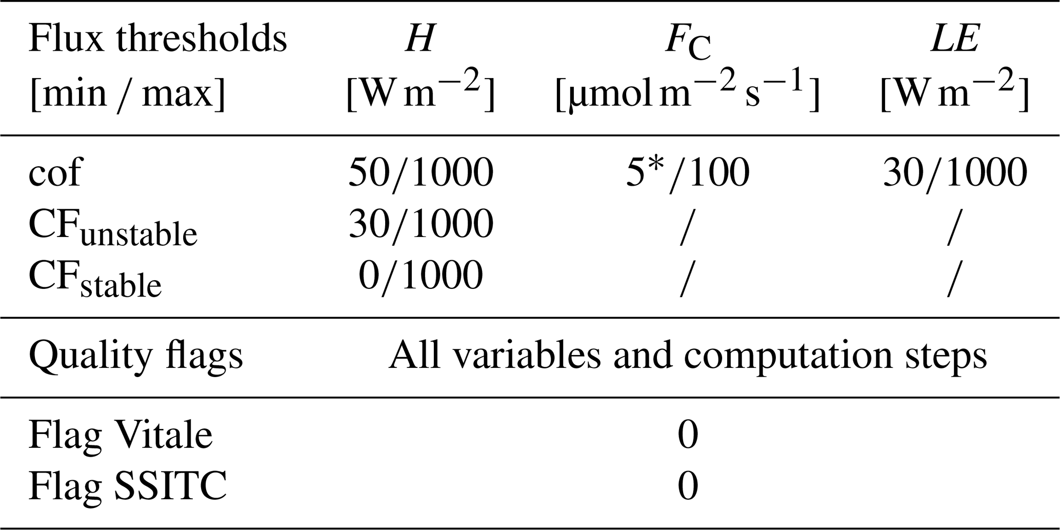
^* Lowered to 2 $\mathrm{\mu }\mathrm{mol}{\mathrm{m}}^{-\mathrm{2}}{\mathrm{s}}^{-\mathrm{1}}$ in an additional run using 8 classes of wind direction, in order to include more data per site.

2.2.3 Automation and standardisation

The spectral analysis and correction procedure described above was developed with the objective of having a unified, automated and standardised approach that could be applied across multiple sites. This turned out to be a challenge, as there were several non-fundamental choices that required the selection of fixed thresholds to be used throughout the procedure. Here, informed decisions were taken after visual inspection of the results of all sites. Thresholds for quality filtering (flux thresholds, quality tests) and fitting ranges, unified across all sites, were chosen to maximise the quality of the data used for the analysis. As a consequence of these choices, one site did not retain a sufficient amount of data to perform the cof analysis, which relies on the most restrictive data selection criteria. This concerned the SE-Deg site for CO₂, where the CO₂ fluxes only rarely exceeded the selected threshold.

Beyond methodological and process-specific considerations, spectral attenuations also depend on technical, setup-related elements such as flow rate, sampling line heating, filter cleanliness and measurement height above the canopy (see Sabbatini et al., 2018 for more details). Changes in any of these parameters should be accounted for and assessed with a separate spectral analysis time window. For the purpose of this work, we considered that these values remained constant throughout the period analysed. While this was the case for the flow rate and line heating (see above), this cannot be strictly guaranteed for filter cleanliness despite regular filter changes. z−d might also be subject to changes due to plant development of fast-growing vegetation but this effect is mitigated by regular adjustment of the measurement height according to the ICOS instructions (Sabbatini and Papale, 2017).

3 Results

3.1 CO₂

Both normalised average temperature and CO₂ concentration spectra and normalised average co-spectra of sensible heat flux and CO₂ flux for all sites were generally well defined, matched quite well in the medium frequencies and showed the expected behaviour in the high frequencies (Figs. B1 and B2). For some sites, especially of the HMH group (black titles in Fig. B2), the presence of white noise on the average gas spectra was observed at a very high frequency, requiring the application of the denoising procedure (Appendix A). This procedure was performed for at least one class of WS at 21 sites (3 out of the 14 LMH, and 18 out of the 23 HMH). Overall, the spectra and co-spectra were of high quality, allowing a robust determination of TFs and associated cofs.

3.1.1 Cut-off frequencies

The ICOS EC setup shows very good spectral performance, with cofs for CO₂ generally above 1 Hz (Fig. 3). The setup being standardised, cofs are expected to fall in the same range for all sites. This is overall the case, with e.g. the mean, standard deviation and interquartile range of half-power cofs for the cospectra (no P21) case of 2.1, 0.56 and 0.82 Hz at a WS of 3 m s⁻¹, and results from both co-spectral and spectral methods showing consistent behaviour, further highlighting the effectiveness of the ICOS setup standardisation.

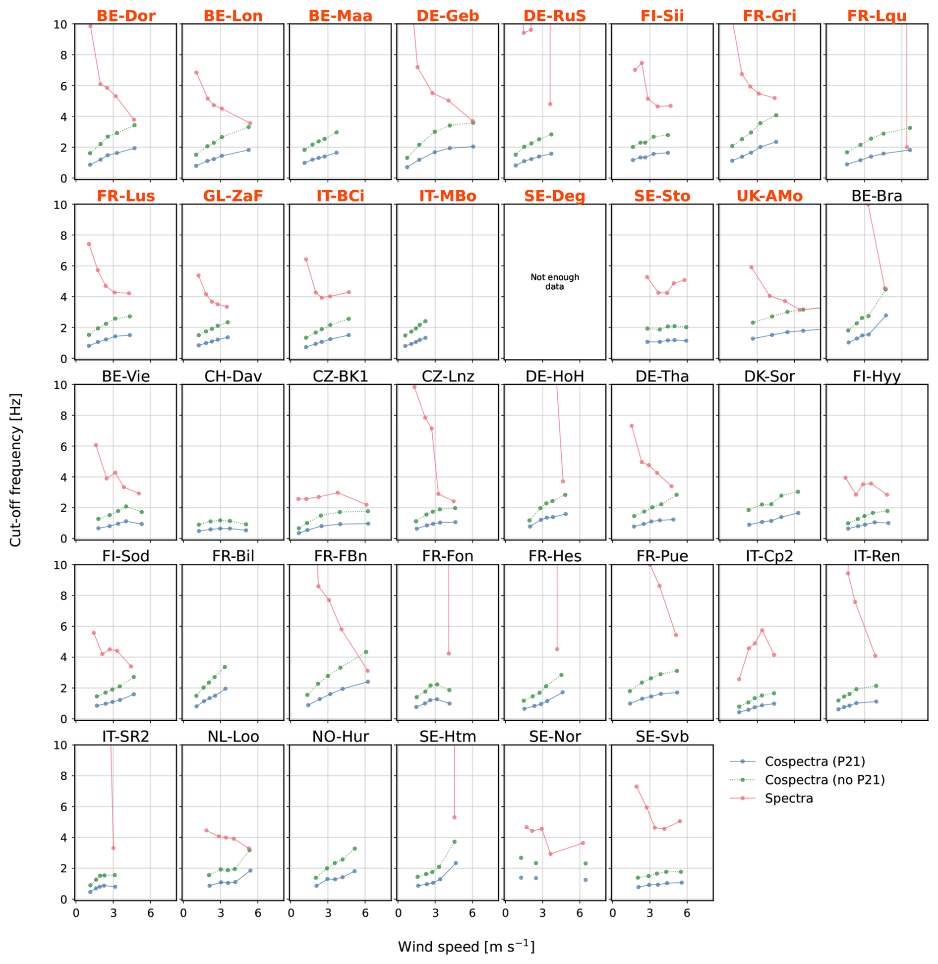
Figure 3 Spectral and co-spectral CO₂ cut-off frequencies as a function of wind speed class average. The red bold titles represent the low-measurement-height sites. This distinction is only presented for symmetry with the rest of the document, as cofs are independent of this parameter. Green lines are the results of fitting the classic Lorentzian to the co-spectral-computed TF, and are presented to ease the comparison with the spectral data (red). Blue cof result from the Peltola-modified fit and are used in the rest of the procedure.

The co-spectral cofs showed a small positive dependence on WS. This is related to their inclusion of the sensor separation effect. In fact, high-frequency losses for sensor separation are expected to decrease with increasing WS, which translates into an increase of cof value.

The spectral cofs are systematically higher than their co-spectral counterparts, consistent with the exclusion of sensor separation from the spectral approach at this stage, and indicating that spectral losses from other sources are minimal with the ICOS setup. The multiple occurrences of spectral cofs outside the displayed range, particularly at low WSs, reflect the difficulty of fitting a TF in these conditions: very little to no loss at high frequency associated with minimal high frequency content yield unstable fit results, always associated with extremely high cofs. The decreasing trend of spectral cofs with WS is therefore likely an artefact. However, this has little practical consequence, as such values correspond to near-zero attenuation and CFs close to 1. The stability of the fit improves at higher WS, where greater high-frequency spectral content results in a better-defined and more robustly fitted TF.

3.1.2 Correction factors

The fully empirical CFs for CO₂ are overall low, resulting in a correction of typically less than 20 % (mean median/interquartile range of $\mathrm{1.054}/\mathrm{0.020}$ and $\mathrm{1.010}/\mathrm{0.003}$ in the unstable case for LMH and HMH, respectively, Fig. 4). This result confirms the efficiency of the ICOS setup in terms of spectral losses, already highlighted with the cof results.

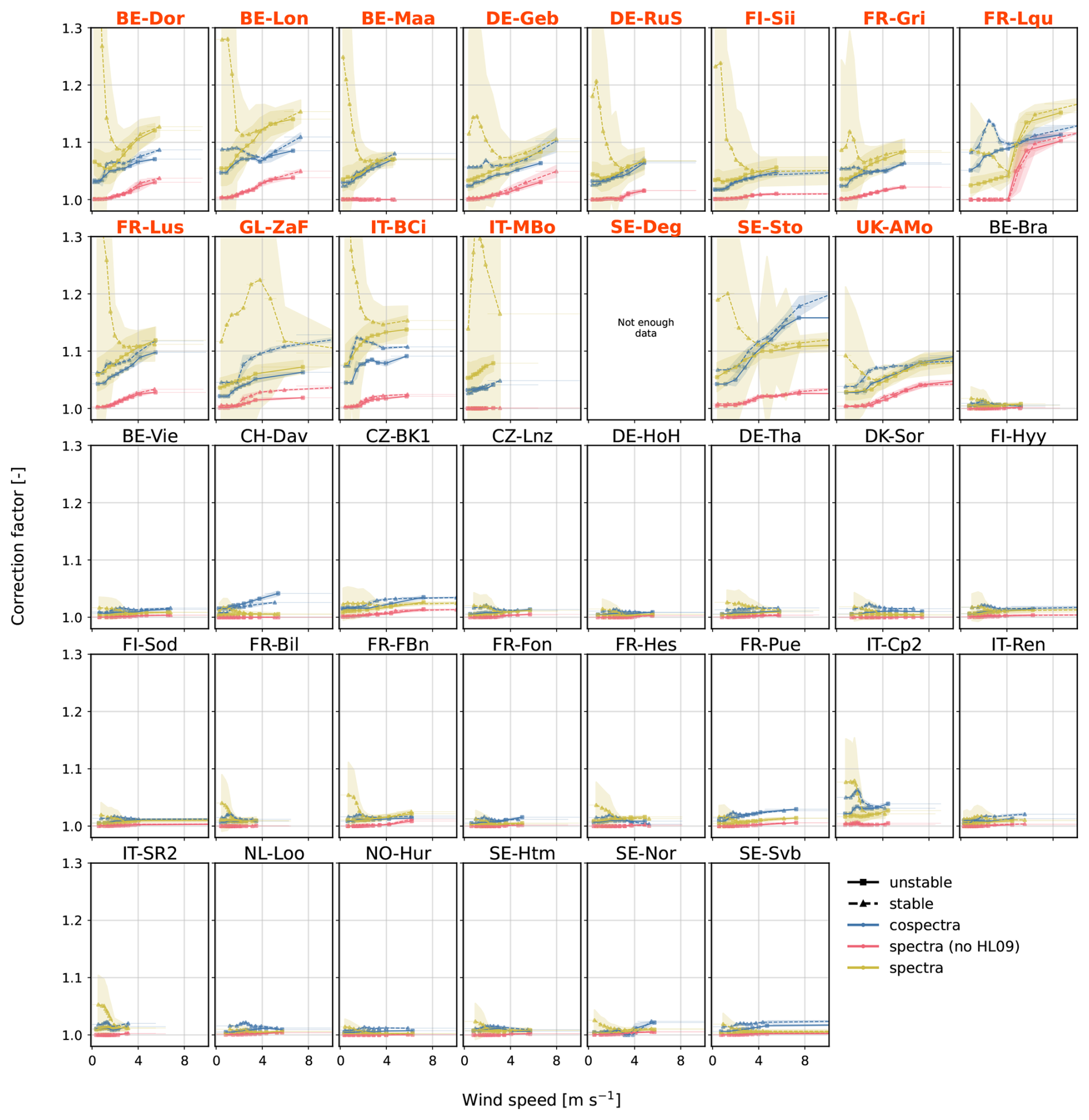
Figure 4 Spectral and co-spectral CO₂ correction factors as a function of wind speed. Data are shown separately for unstable (squares) and stable (triangles) conditions. For the spectral approach, the orange lines show the final CFs including the sensor separation term. The shaded area around the lines corresponds to ±1 SD around the mean. The red bold titles represent the low-measurement-height sites.

Co-spectral CFs (i.e. co-spectra computed using the co-spectral approach) are larger than spectral ones when the latter do not include the sensor separation term (Fig. 4, blue and red lines, respectively). This pattern is consistent across sites, in line with the cof results, and is a consequence of the inclusion of the sensor separation term in the co-spectral approach only. The addition of the theoretical sensor separation term to CF_sp (yellow lines in Fig. 4) results in higher total CFs for the spectral than for the co-spectral approach, at least for LMH, making the sensor separation term the dominant contribution to the correction for this gas and setup, especially at low WSs.

A marked dependence to z−d, stability and WS is observed for both approaches. LMH (red bold titles in Fig. 4) have larger CFs than higher sites. This is expected, as low sites, with more content in high frequencies, lose more signal than the high ones for the same cof (lateral shift of the reference co-spectra peak to higher frequencies for LMH). The z−d dependence is also explicitly included in the sensor separation theoretical equation (Appendix E). Amplified differences between the spectral and co-spectral CFs for LMH are observed.

Stable atmospheric conditions show higher CFs than unstable conditions for both approaches. The dependence on atmospheric stability is explicitly expressed in the theoretical sensor separation equation (Appendix E), and taken into account in the empirical approach by computing CF separately for stable and unstable conditions. The effect is minor for the fully empirical CFs (co-spectra), with some larger differences visible at very low WSs, generally linked to very stable conditions. However, the full spectral approach shows a strong dependence on the stability parameter for stable conditions (dashed yellow line in Fig. 4), leading to larger differences between the methods in such conditions.

Finally, both methods show a trend of increasing CF values with WS.

3.1.3 Fluxes

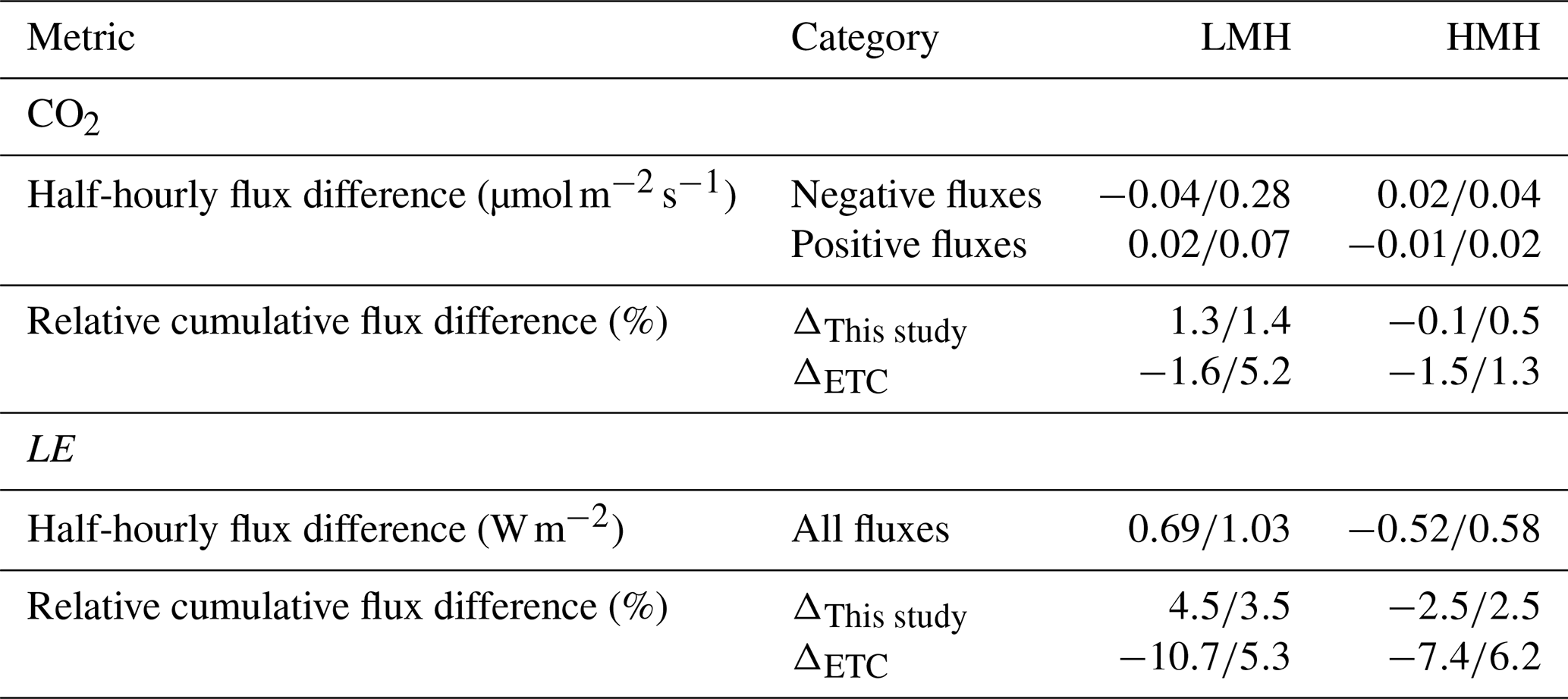
First, there are very small to no differences between the half-hourly fluxes corrected by the two methods for HMH (mean median/interquartile range of $\mathrm{0.02}/\mathrm{0.05}$ and $-\mathrm{0.01}/\mathrm{0.02}\mathrm{\mu }\mathrm{mol}{\mathrm{m}}^{-\mathrm{2}}{\mathrm{s}}^{-\mathrm{1}}$ for negative and positive fluxes, respectively), and very small ones for LMH (mean median/interquartile range of $-\mathrm{0.08}/\mathrm{0.27}$ and $\mathrm{0.02}/\mathrm{0.09}\mathrm{\mu }\mathrm{mol}{\mathrm{m}}^{-\mathrm{2}}{\mathrm{s}}^{-\mathrm{1}}$) (Fig. 5, Table 2). This reflects the results of unstable CFs, which is expected as u^* filtering was applied and largely removes stable data. Then, when differences are present, they confirm the CF results in their sign, with spectral fluxes generally being bigger (in absolute values) than co-spectral ones.

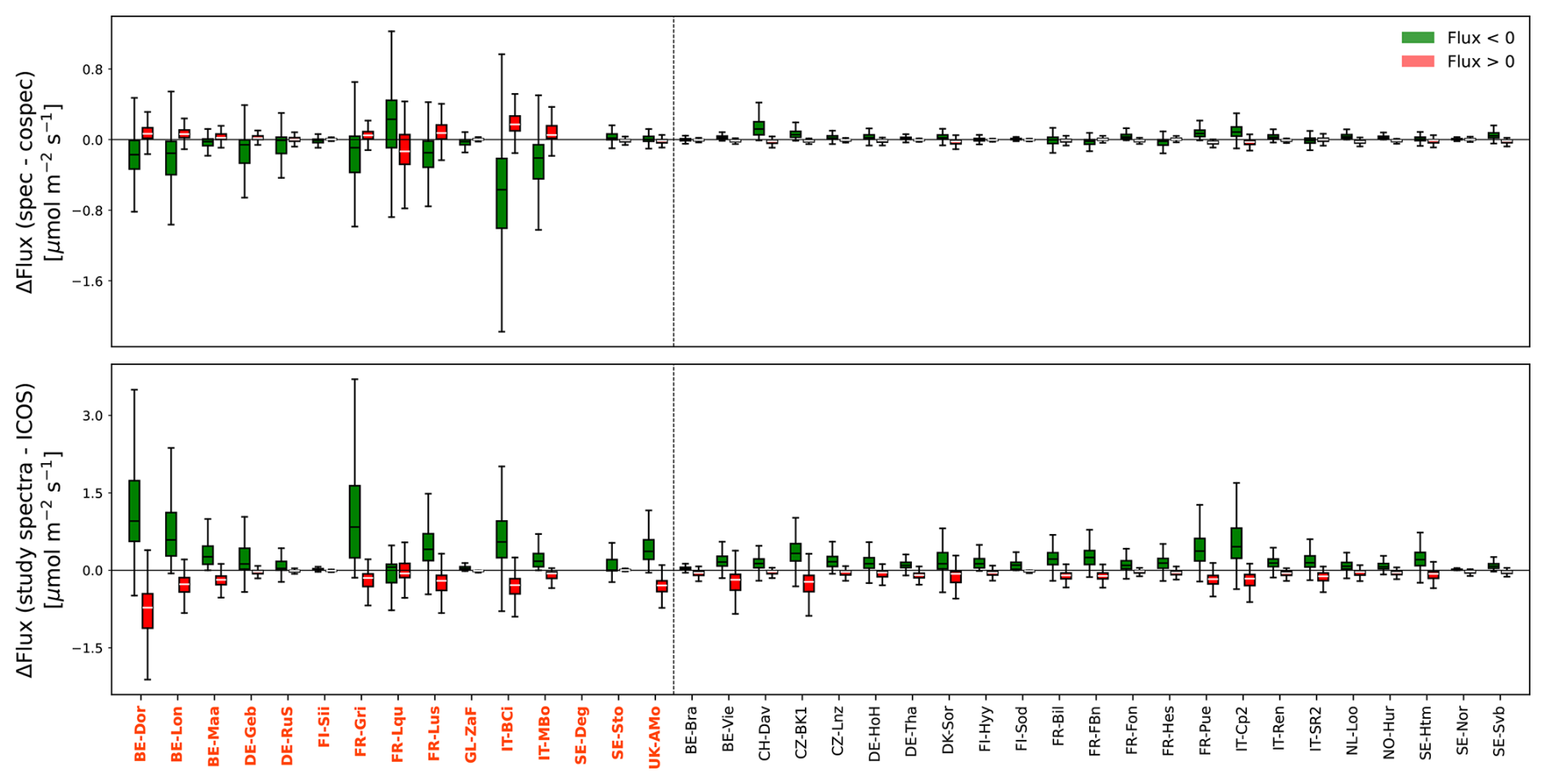
Figure 5 Boxplot of CO₂ half-hourly flux differences between the two spectral correction methods, separately for negative and positive fluxes (top) and same figure for the differences between this paper spectral correction method and the ICOS one (bottom). Only quality and u^* filtered fluxes were selected. Box frame = 25 %–75 % interquartile range (IQR), bold line = median, whiskers = 1.5 × IQR. The red bold labels represent the low-measurement-height sites. Note the different scales on the y axes.

These half-hour flux differences translate into relative cumulative flux differences of maximum 4.8 %, with 21 sites out of 23 under 1 % for HMH, and maximum 2.1 %, with 8 sites out of 14 under 1.5 % for LMH (Fig. 6, Table 2 and Appendix C). Note that cumulative CO₂ fluxes undergo an offsetting process due to the presence of both negative and positive values, which can result in partial neutralisation of differences between methods.

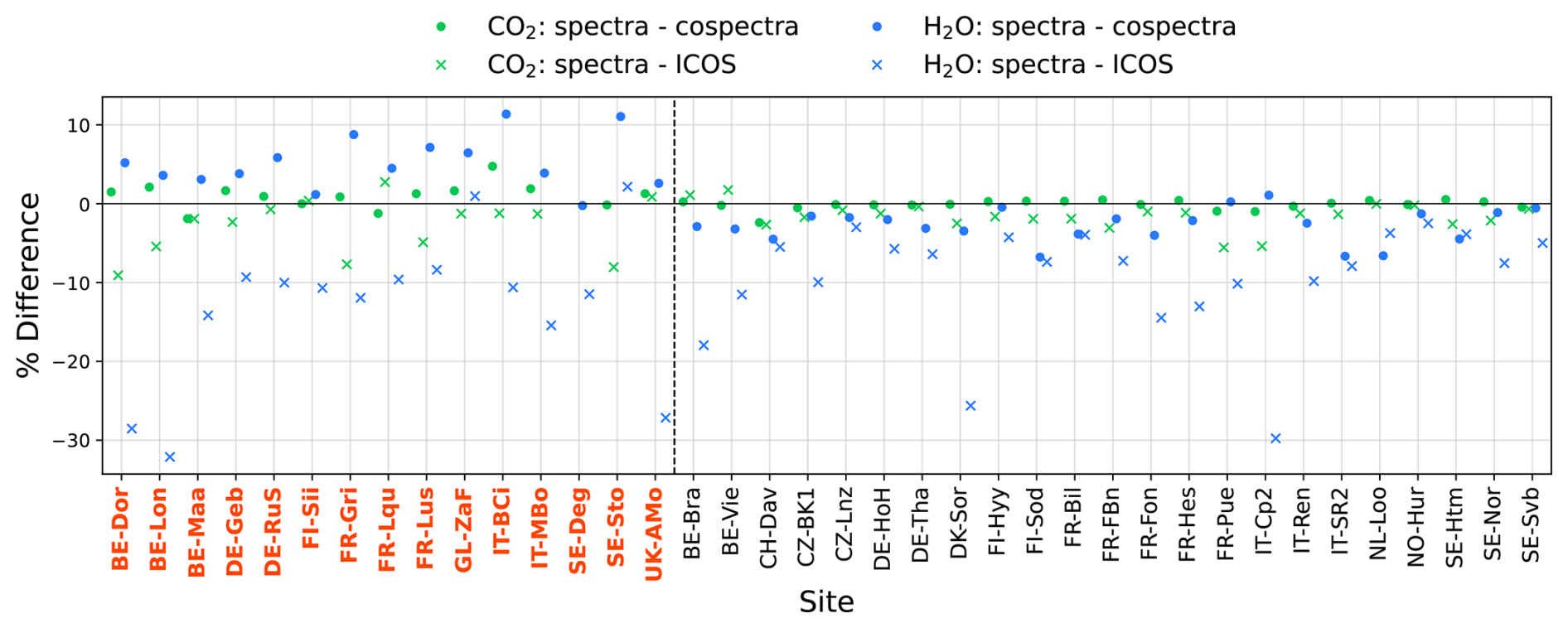
Figure 6 Percentage differences in CO₂ and H₂O cumulated fluxes between the two spectral correction methods and same figure for the differences between this paper spectral correction method and the ICOS one. The absolute cumulative fluxes were used. The red bold titles represent the low-measurement-height sites.

Because the ICOS pipeline for frequency corrections relies on a spectral approach, the corrected fluxes are expected to match those obtained using the spectral method implemented in this study. However, this is generally not the case, with differences between the ICOS pipeline and the spectral method implemented here typically larger than for the co-spectral-spectral pair (Figs. 5 and 6). For example, the IQR of the cumulative flux differences reached 5.2 % for LMH (Table 2). Possible causes of these differences are identified and discussed in Sect. 4.4.

Table 2 Summary statistics for CO₂ and LE flux corrections differences between the two spectral correction methods (spectra−co-spectra). In each case the mean median/interquartile range of the metric are provided.

3.2 H₂O

Normalised average spectra and co-spectra for H₂O are generally well-defined and not noisy (Figs. B3 and B4). However, H₂O spectra show an unexpected behaviour at low frequencies, where they are systematically higher than the ideal ones. The two curves then cross, with the real spectra decreasing faster than the ideal in higher frequencies. It results in a TF that continuously decreases with increasing frequency, without having the typical plateau that precedes the fall linked to spectral losses (not shown). This behaviour is present for all sites for spectra and sometimes for co-spectra as well. It generally worsens with increasing RH values and makes it more challenging to perform a robust fitting procedure, as the Lorentzian equation expects a no-filter zone before the fall with the increasing frequency. This behaviour is acknowledged here, although the Lorentzian formulation is still used for fitting, as it represents the most widely adopted approach, consistent with the CO₂ case. Moreover, similar deviations from the idealised TF have been reported in a range of atmospheric conditions and are not specific to the ICOS sites and set-up considered here. A more detailed discussion on this aspect is provided in Sect. 4.2.

Moreover, as it was the case for CO₂, several occurrences of white noise are visible on real spectra at high frequency, which implies that the denoising procedure was necessary before cof computation. Indeed it was found that denoising was activated for at least one RH class in 32 sites (10 out of 15 and 22 out of 23 LMH and HMH respectively), with more occurrences observed for high RH and WS classes.

3.2.1 Cut-off frequencies

The dependence of cof to both RH and WS was investigated through a double classification in RH and then WS classes. The former was found to be dominant, with the variability inside each RH class being quite low, as shown by the small error bars in Fig. 7. The expected dependence of cof to RH is met for all stations (Fig. 7) and is modelled as a negative exponential function, with satisfactory fit results as presented in Appendix D. Overall, the same order of magnitude is found across sites, with cof generally well below 1 Hz for dry conditions and decreasing to 0.1 Hz for high humidity conditions. There is a general coherence in the cof results among sites for similar humidity conditions (e.g. mean median/interquartile range of $\mathrm{0.236}/\mathrm{0.036}$ Hz at 60 % of RH for all sites and with the cospectral P21 approach), supporting once again the effectiveness of the standard ICOS setup standardisation. The values found are lower than for CO₂, which is in line with the higher spectral losses impacting H₂O measurements linked to the adsorption/desorption processes affecting the water molecules in the sampling tube.

As expected, co-spectral cof (from P21 fitting) are generally lower than spectral ones, but compared to CO₂ they are much more similar between the two methods, suggesting that the main sources of spectral losses are common to both approaches. It is observed that co-spectral cofs fitted with the non-modified Lorentzian are systematically higher than the spectral values. This outcome is likely linked to the inability of the non-modified Lorentzian to account for the low-pass filtering induced by the time-lag estimation method used, which results in a systematic underestimation of the attenuation (Peltola et al., 2021).

The absence of extreme relative humidity values is true for all sites, with the highest RH class mean rarely exceeding 90 %. This result is inherent to the use of flux filtering thresholds that remove periods with small LE fluxes, generally corresponding to high humidity conditions and to the use of equal population bins. In practice, cof found for the highest RH classes are generally stabilised (Fig. 7), suggesting that the error on the true cof for unaccounted high humidity conditions would be minor. Moreover, LE fluxes at high RH are generally small, which minimises the impact of this bias on the final results.

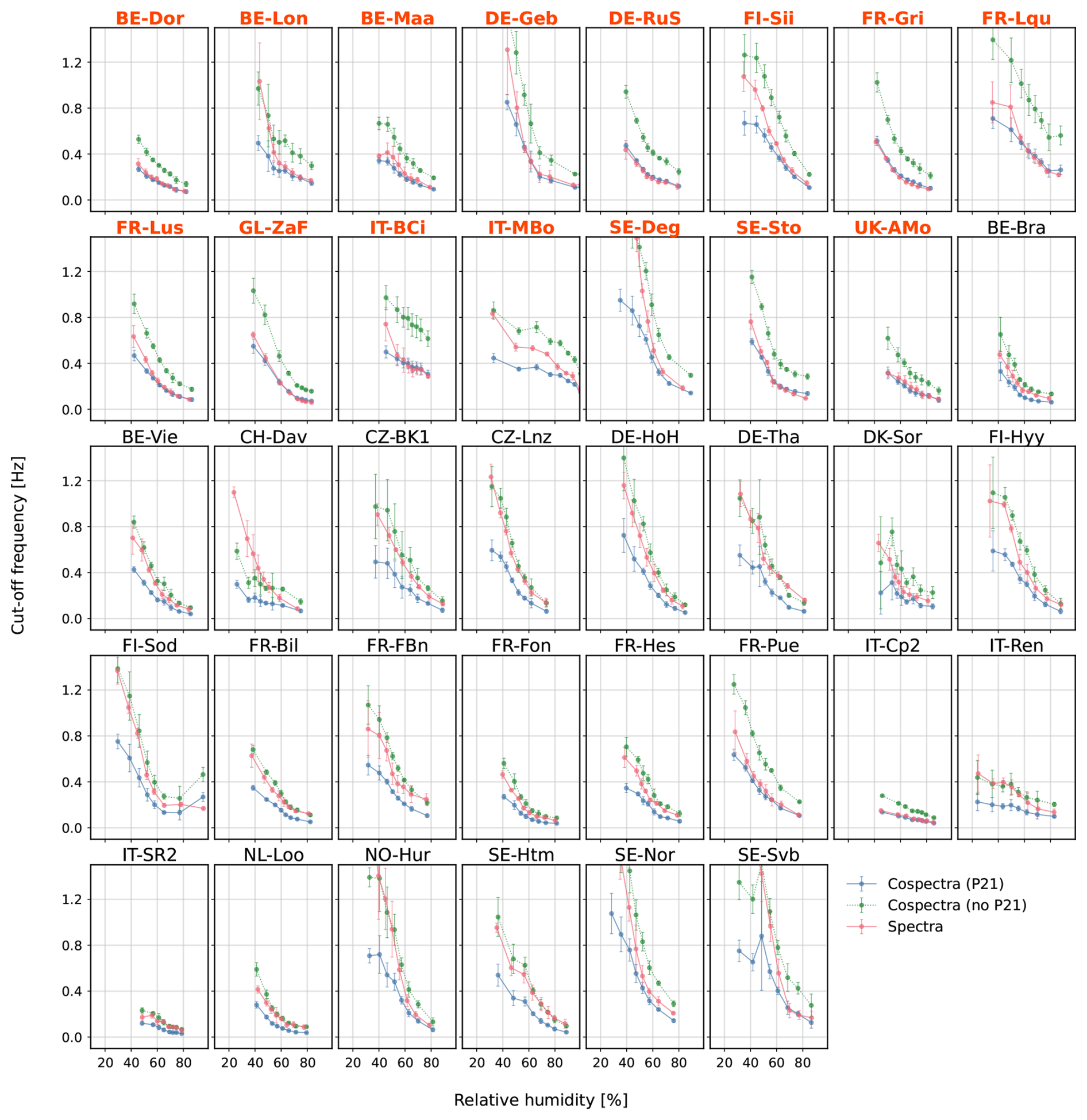
Figure 7 Spectral and co-spectral H₂O cof as a function of relative humidity. Each data point is computed as the average across the 4 WS classes in each RH class. The error bars represent the standard deviation of the wind-speed-class means within each RH class, thus illustrating the variability within each RH class across different WSs. The red bold titles represent the low-measurement-height sites.

3.2.2 Correction factors

In line with the cofs found, H₂O CF values are higher than for CO₂, and both co-spectral and spectral methods yield very similar results (blue and red lines in Fig. 8). Because of the higher relative importance of other sources of spectral losses, the addition of the sensor separation term has a relatively minor impact on H₂O correction and does not alter the spectral results.

In accordance with CO₂ results, the highest CFs are found in LMH. It also appears more clearly that co-spectral CFs for HMH are bigger than the final spectral ones, which is a consequence of both the small cof (Fig. 7) and the low sensor separation term values that have almost no effect on spectral CF.

The impact of stability conditions is more marked for H₂O, and results in a systematically higher CF for stable conditions than unstable, for all methods. Combined with the z−d effect, the highest differences between stable and unstable results appear in the LMH. The low cof values explain the importance of this effect for H₂O, for which even a small change in the co-spectrum position can lead to significant differences in signal loss.

Consistent with CO₂ results, a CF dependence to WS is found for both methods and stability conditions (in Fig. 8 for RH values between 55 % and 65 %). However, it is amplified by the fact that the H₂O cof does not appear to depend on WS, so that a constant (small) cof is applied to the shifting co-spectrum, thus yielding higher CFs. The additional dependence on RH, already observed in the cof results, is confirmed (Figs. D2 and D3) for both methods.

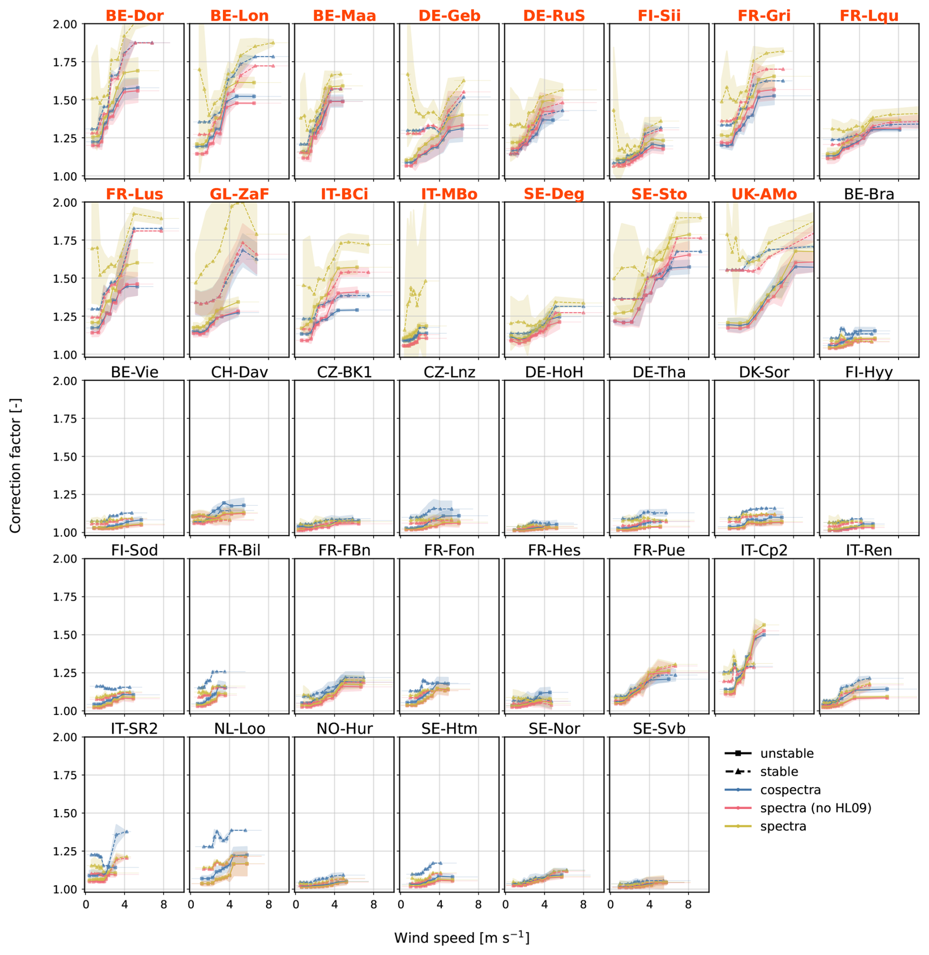
Figure 8 Spectral and co-spectral H₂O correction factors as a function of wind speed, for relative humidity between 45 % and 55 %. Data are shown separately for unstable (squares) and stable (triangles) conditions. For the spectral approach, the orange lines show the final CFs including the sensor separation term. The shaded area around the lines corresponds to ±1 SD around the mean, a spread that's linked to the additional dependence of water CF to RH. The red bold titles represent the low-measurement-height sites.

3.2.3 Fluxes

As for CO₂, the impact of the CFs on the final fluxes is assessed on the latent heat (LE) half-hourly fluxes (Fig. 9). The mean median/interquartile ranges of the flux difference between the spectra and the co-spectra values are $\mathrm{0.69}/\mathrm{1.03}$ and $-\mathrm{0.52}/\mathrm{0.58}$ W m⁻² only for LMH and HMH, respectively (Table 2). However, they reach $\mathrm{2.48}/\mathrm{2.48}$ and $-\mathrm{1.14}/\mathrm{1.42}$ W m⁻² when selecting only the daytime fluxes (not shown).

The relative cumulative flux differences were bigger than for CO₂, reaching 4.5 % for LMH and −2.5 % for HMH (Table 2, Fig. 6 and Appendix C) and with 3 sites reaching values higher than 7 % and only 15 sites out of 38 having differences lower than 2 % (Fig. C2). It should be noted that, water fluxes being mainly positive, no compensation effect is present, and differences on cumulative sums are fairly representative of the half-hourly differences (confirmed by half-hourly linear regression results, not shown). The LMH and HMH-logic is less marked but consistent with the previous results. In particular, as observed for CFs, in LMH spectral-corrected fluxes are higher than the co-spectral ones, while the opposite is true for HMH.

In line with CO₂, the ICOS-computed H₂O fluxes are expected to match the spectral-corrected fluxes, which is however not the case, with differences largely exceeding the inter-method comparison (Fig. 6 and Appendix C). For example, the median and IQR of cumulated flux differences reached −10.7 % and 5.3 % for LMH, respectively (Table 2).

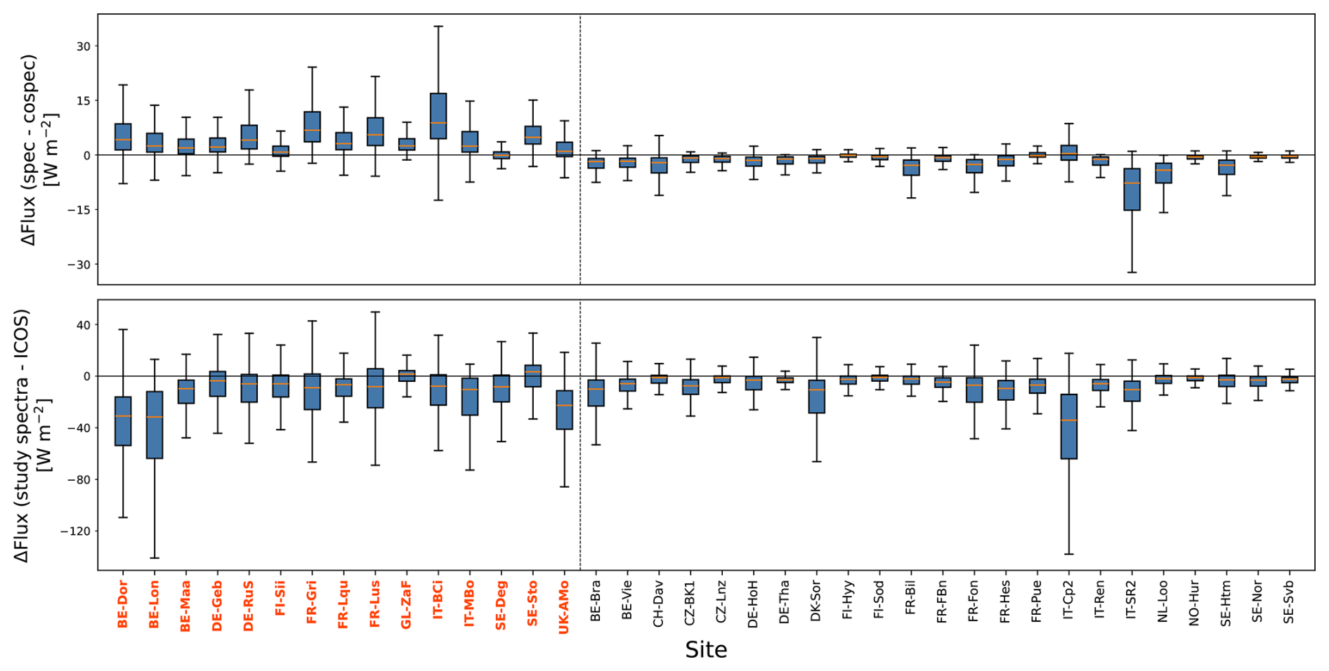
Figure 9 Boxplot of LE half-hourly flux differences between the two spectral correction methods (top) and same figure for the differences between this paper spectral correction method and the ICOS one (bottom). Only quality, u* filtered and daytime fluxes were selected. Box frame = 25 %–75 % interquartile range (IQR), bold line = median, whiskers = 1.5 × IQR. The red bold labels represent the low-measurement-height sites. Note the different scales on the y axes.

3.3 Sensor separation term

The impact of the sensor separation term has been highlighted in the gas-specific CF results (Sect. 3.1.2 and 3.2.2). This factor is identical for any gas for a given setup and atmospheric condition. Therefore, its relative contribution depends on the importance of other sources of spectral loss, which are minimal for CO₂ but more substantial for H₂O, making the sensor separation term the main contribution to the total CF for CO₂ (Fig. E2).

The wind direction effect is proper to the sensor separation term, as no other source of spectral loss depends on it, and its impact on CFs is therefore further assessed for both methods. The focus is on CO₂ results, as for H₂O the RH effect was found to dominate over any other dependency.

To isolate the wind direction effect, 8 classes of WD were used to compute cofs and CFs for both approaches, selecting unstable conditions and data with WSs between 2 and 3 m s⁻¹ (Fig. 10). Because of this additional data filtering, some station datasets had not enough data for a robust computation and were excluded from the analysis. In these conditions, the directional effect dominates the full spectral CF, as expected. Interestingly, a trend with wind direction is observed in the co-spectral results as well, experimentally confirming the model assumption. The magnitude of co-spectral CF is systematically smaller than the theoretical one, but generally in phase with the expected minimum and maximum zones (Fig. 10).

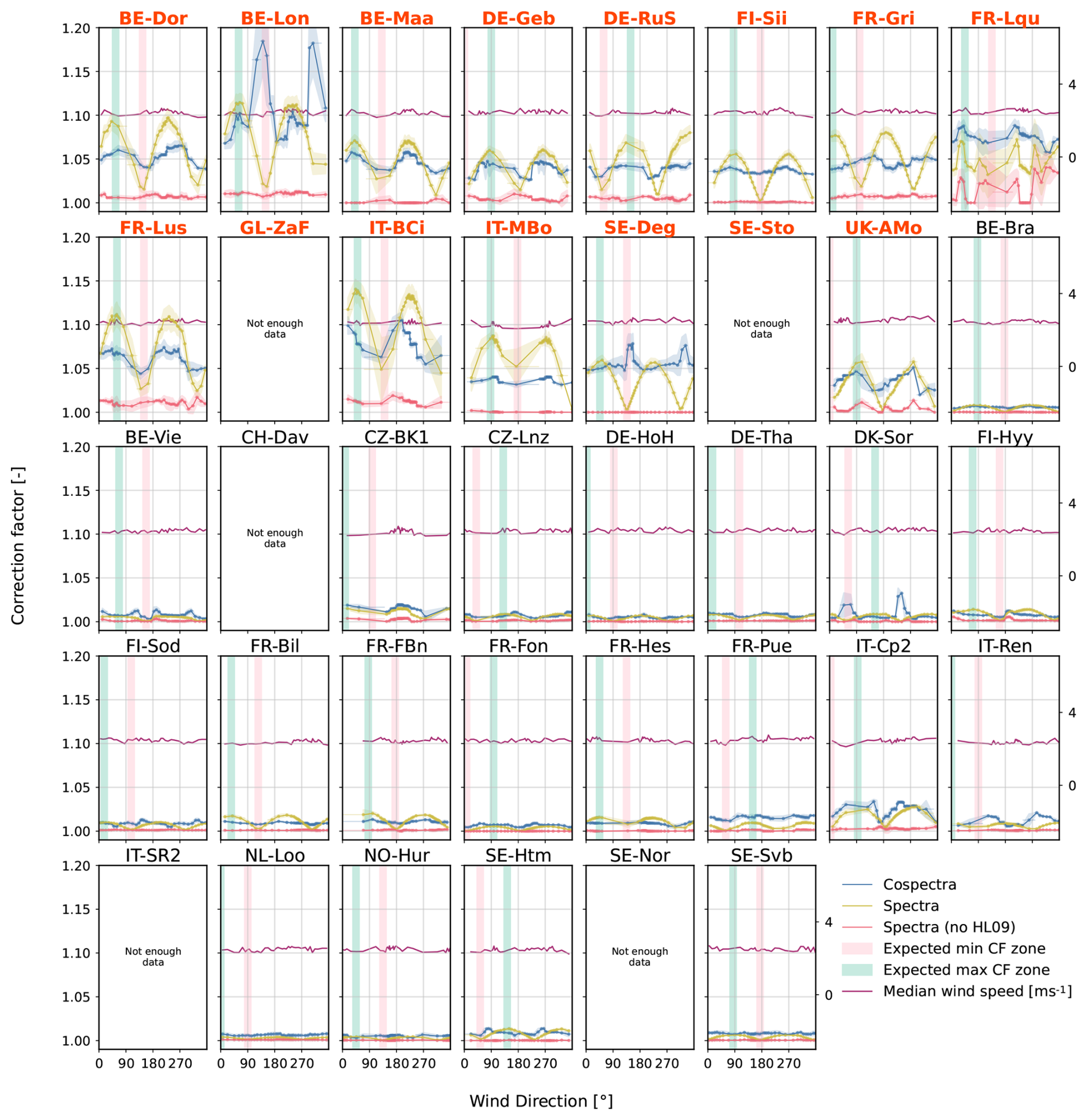
Figure 10 CO₂ co-spectral and spectral correction factors as a function of wind direction, grouped in equal-number-of-points bins. Data are filtered for unstable conditions and wind speeds from 2–3 m s⁻¹. The red bold titles represent the low- measurement-height sites.

Finally, a systematic pattern of WSs with wind direction is observed across sites (not shown), which results in a cross-dependence that makes it harder to determine which term is the main driver of the CF dependence.

4 Discussion

4.1 Limited but still significant and systematic differences between correction methods

The comparison of spectral and co-spectral approaches has been presented through the impact on cut-off frequencies, correction factors, half-hourly fluxes and, finally, cumulative fluxes (not gap-filled). The results show that the differences between the methods for CO₂ fluxes are systematic, the spectral method having higher CFs and thus amplifying the fluxes. The difference is always very low for HMH due to limited high-frequency signal content and therefore overall very low CFs. It is higher, but still limited, for LMH sites, the worst case being only 0.04 $\mathrm{\mu }\mathrm{mol}{\mathrm{m}}^{-\mathrm{2}}{\mathrm{s}}^{-\mathrm{1}}$ for mean median negative fluxes (Table 2) and the impact on cumulative fluxes is only on average of 1.3 %. It can, however, reach higher values for specific stations (e.g. up to 0.56 $\mathrm{\mu }\mathrm{mol}{\mathrm{m}}^{-\mathrm{2}}{\mathrm{s}}^{-\mathrm{1}}$ for IT-BCi, and 4.8 % on cumulative fluxes).

The differences get worse for LE, with the spectral correction overestimating the co-spectral one by 2.48 W m⁻² on average for LMH half-hourly fluxes and by 4.5 % on cumulated fluxes. The overestimation is even reaching 5 %–10 % for 9 out of 38 sites (Fig. 6).

The same order of magnitude for differences was found by Polonik et al. (2019) in their single site study and here the differences are investigated in terms of dependencies, magnitude and causes, and placed in the larger framework of spectral correction approaches assumptions and limitations.

4.2 Methodological differences and underlying causes

There are fundamental differences in the theory underlying the spectral and co-spectral methods to be considered and discussed.

The results across all sites confirm a strong dependence of the CF on the cof, which stresses the importance of correctly characterising the system attenuation behaviour, before combining it with the spectral content to get the CFs. Its computation depends on the quality of the (co-)spectra used to derive the empirical TF, as well as on the choice of the TF to be fitted to the data.

The use of Eqs. (1) and (2) to derive the TF relies on the assumption of spectral similarity in the low frequencies. This hypothesis is generally accepted and widely used in similar correction procedures, in particular when the half-hourly variability that could undermine its validity is levelled out by the use of averages over very specific atmospheric conditions (Emad, 2023). While well observed for CO₂, including in this work, multiple works have highlighted an apparent lack of spectral similarity between H₂O and temperature spectra (Wintjen et al., 2020). The observed shapes of the H₂O spectral averages used in our work follow those findings (Fig. B4), with a lack of spectral similarity in the lower frequencies that appears to worsen with increasing RH (and thus attenuation, not shown), and is more marked for spectra than co-spectra (Appendix B). Such dissimilarity has been investigated in various studies and was found to be systematic for water vapour fluxes at low frequencies due to different transport processes affecting the two variables (Asanuma et al., 2007). Besides, in their work, Wintjen et al. (2020) link a similar behaviour of gas spectra in the low frequencies to the presence of red noise (i.e., noise dominated by slow, correlated variations at low frequencies). In either case, this result challenges the validity of using spectra for the correction of water vapour attenuation, and the results should be interpreted keeping this limitation in mind.

The attenuation is approximated by a first-order filter in the shape of a Lorentzian (Eq. 3). Although widely used in the literature (Su et al., 2004; Foken et al., 2012b; Fratini et al., 2012), many argue that this simple response function does not reflect the complexity of the EC system, and therefore cannot correctly describe its whole damping behaviour (Polonik et al., 2019; Wintjen et al., 2020; Emad, 2023). This is particularly true for H₂O, for which other shapes of TFs (e.g. Gaussian) have been suggested (De Ligne et al., 2010). Similarly, the inclusion of a square root in the TF definition is still debated (Emad, 2023), and in particular is included in the co-spectral approach based on work relying on a Lorentzian TF shape (Peltola et al., 2021). The choice of TF shapes and the impact it can have on the spectral-co-spectral comparison is hard to predict and should therefore be tested systematically for both methods and gases.

In addition to these general considerations, there are method-specific effects that should be acknowledged. Firstly, the co-spectral approach requires a proper time-lag estimation, the recognition of the low-pass-filtering-induced time lag and consequent phase-shift, and the inclusion of this effect in both the cof and CF estimations. It is included in this work through the use of $\sqrt{\text{TF}}$ (in both Eqs. 4 and 5), which is however an approximation that could fail under very strong attenuations (Peltola et al., 2021). Co-spectral data are also generally considered noisier and more sensitive to contamination from bad measurements than spectral data, since they depend on two variables (Ibrom et al., 2007). We observed that thanks to very selective high-quality filtering of the data, this risk can be minimised, resulting in good quality, noise-free co-spectra (Figs. B1 and B3). In rare instances where lower-quality data pass all screenings, the impact generally depends on total attenuation. In our analysis, it resulted in co-spectral outputs being more impacted than spectral ones for CO₂. This is because the spectral cofs, not including the sensor separation effect, are so high that a lower resolution of the TF has little to no impact, whereas this is not the case for co-spectra.

On the other hand, the presence of noise is observed for spectra, mostly in the highest frequencies when the real signal is low (Figs. B2 and B4). Using an automatic procedure (described in Appendix A), noise was found and removed at 58 % and 84 % of sites for CO₂ and H₂O, respectively. In line with similar observations (Ibrom et al., 2007; Aslan et al., 2021; Wintjen et al., 2020), these results confirm that denoising plays a central role in the spectral method, and that addressing the limitations of the current procedure (e.g. assumption of white noise) and stabilising a robust approach are necessary (Aslan et al., 2021).

Finally, we showed that CO₂ attenuation is dominated by the sensor separation effect, the theoretical term that corrects for this effect constituting on average 89 % of the total spectral CF (across sites and for unstable conditions) (Fig. E2). For the spectral approach, this means that the final CF rely heavily on the theoretical equation defining this specific term. This is questionable for an approach that is initially intended to be mainly experimental. In these conditions, the applicability of the chosen theoretical approach to define the sensor separation CF should be addressed. The method developed by Horst and Lenschow (2009) uses an exponential model to estimate the attenuation as a function of the co-spectral peak frequency (parameterised according to stability) and the distance between the sensors (depending on wind direction). If the modelled peak frequency does not reflect the turbulent characteristics of the site, the estimated attenuation could be biased (Mammarella et al., 2016). Here, a comparison with the co-spectra results revealed that CF_HL09 are far more sensitive to atmospheric stability than the experimental CF, reaching unrealistically high values under stable conditions (Fig. 4). This is consistent with findings from other studies (Mammarella et al., 2016; Polonik et al., 2019), and whilst the consequences on the fluxes surviving the traditional flux filtering are minimised (the u^* filtering removes most stable conditions), it is considered methodologically questionable. Moreover, a dependence of co-spectral CF on wind direction was found, generally in phase but with a smaller amplitude than the modelled behaviour (Fig. 10). This result experimentally confirms the theoretical framework, though only partially its application, and validates the co-spectral method in its ability to account for all sources of attenuation. It further suggests that explicitly including the directional effect in the co-spectral approach could improve CF computation. However, in practice, this is not always feasible: the additional classification, combined with site-specific wind roses, would further fragment the dataset, potentially leaving insufficient data to reliably apply the procedure. Given this limitation – and considering that a dependence between WD and WS is also observed (Fig. E3), and that WS distribution at a given site is typically broader and more uniform than that of wind direction – WS classification alone is deemed sufficient for the co-spectral approach.

Common to the two approaches is the choice of the reference co-spectrum. Here, the fully empirical method is used, and therefore the measured sensible heat co-spectrum is considered ideal. However, it should be noted that what to use as an unattenuated reference is an ongoing discussion in the literature, with works suggesting that the empirical choice is not the wisest and that theory-based parametrisations of ideal co-spectra should be used (Smidt et al., 2025).

All the limitations presented above can lead to uncertainties at different levels of the correction procedure. The errors linked to this effect are systematic, and an estimation of the sources and magnitude of those uncertainties at each step of the correction procedure is therefore necessary to assess the significance of the differences found.

Overall, our results show spectra characterised by a lack of spectral similarity in the low frequencies for H₂O, increasing with RH, and by the presence of (assumed) white noise in the high frequencies, also for strong attenuations mostly. Even if the latter is accounted for with an ad hoc procedure, both contribute to increase the uncertainty in the TF definition and cof computation. On the other hand, concerns related to the quality of the co-spectral data are minimised, leading to stable results across sites. In this context, and for the very specific ICOS standard setup measuring CO₂ and H₂O, we recommend using the co-spectral approach.

4.3 Dependence on gas and atmospheric conditions

Differences between methods were found to be more important for H₂O than for CO₂, at least on cumulative fluxes (Table 2 and Figs. C1 and C2). In this specific metric, the absence of positive/negative offset effects compared to CO₂ can play a role. But more important differences between methods can already be found on CFs (Figs. 4 and 8). This is also due to higher CFs for H₂O. While CO₂ flux attenuation is dominated by the sensor separation effect, adsorption and desorption of water molecules on the sampling tube seem to dominate the high-frequency losses for H₂O (Fig. 7). This phenomenon results in a strong dependence to atmospheric RH and overall larger attenuations than for CO₂, both observations in line with the existing literature (Ibrom et al., 2007; Mammarella et al., 2009; De Ligne et al., 2010; Fratini et al., 2012). For the spectral approach, these effects translate in a decreased relative dependence of the final spectral-computed CF to sensor separation (Fig. E2).

For both gases, differences between methods increase with stability and WS, and decrease with measurement height (Figs. 4 and 8). It is known that these variables are linked to a shift of the reference co-spectrum peak towards the higher frequencies (for an increase in $\frac{z}{L}$ and WS and a decrease in z−d) (Kaimal et al., 1972; Foken et al., 2012a), which yields greater CFs for the same cof and therefore an amplification of the differences between methods.

Atmospheric stability, and in particular the occurrences of stable conditions, play an important role through a double effect. Firstly, the shift of the reference co-spectrum and its consequences mentioned above are observed on both methods and gases, but the level of the impact on the CFs and then fluxes depends on the cof value – the smaller the cof, the larger the impact of a shift towards the high-frequency range. Secondly, for the spectral approach only, a direct effect arises from the theoretical sensor separation term, which is highly sensitive to $\frac{z}{L}$ under stable conditions. This leads to systematically large final CFs at low WSs, typically associated with stable episodes (Figs. 4 and 8) and that cannot be reproduced by the fully experimental co-spectral approach.

The analysis of the impact of spectral corrections on fluxes is performed on u^*-filtered fluxes. The filtering is applied to reflect the standard EC-flux post-processing pipeline that requires the removal of non-representative fluxes prior to their gapfilling (Reichstein et al., 2005; Pastorello et al., 2020). In practice, the removal of conditions considered as not fully turbulent largely filters stable conditions (Aubinet et al., 2000). Therefore, one major source of differences is removed, and, in the end, the impact of stable conditions on the final fluxes is minor (Figs. C1 and C2).

In line with the work by Reitz et al. (2022), higher measurement heights above displacement level (z−d) yield lower CFs, which is again attributed to the shift of the reference co-spectrum towards higher frequencies. This effect is so important that, for stations that were categorised as “high-measurement-height sites” (23 out of 38), and that in practice cover all forest stations, CFs are so low that the high-frequency loss correction could probably be simply skipped and differences between methods for CO₂ are so low that they cannot be appreciated (Fig. C1). The situation is slightly different for H₂O, where if the impact of z−d is clear on CF results (Fig. 8), it is less so on (cumulative) fluxes (Figs. 9 and C2), where differences between methods are enhanced by the larger magnitude of the CFs, including for HMH. These results highlight the importance of installing EC systems at the highest possible position, subject to considerations on the extension of the footprint in the target surface (Munger et al., 2012; Rebmann et al., 2018), and at the same time stresses the importance of an accurate correction procedure for towers measuring close to the canopy.

In this work, a WS classification is applied at the cof level to account for the dependence of cof on WS induced by sensor separation, as theorised by Moore (1986). Although this expected dependence is typically not accounted for in the literature, it is systematically observed for CO₂ in our dataset, where the co-spectral cof increases with WS (Fig. 3). This behaviour is consistent with the dominance of the sensor separation term in the overall correction. The resulting dependence of CFs on WS reflects the interplay of two competing effects. On the one hand, the sensor separation contribution is not expected to introduce a strong WS dependence, as the shift of the reference co-spectrum peak to higher frequencies is offset by the corresponding adjustment in cof. On the other hand, other sources of spectral losses, associated with a constant cof, should lead to a positive relationship between CF and WS. In the co-spectral approach, these two effects are accounted for simultaneously, yielding the observed trend. For the spectral approach, the separation of these contributions would suggest a stronger dependence of the non-sensor-separation term on WS (red lines in Fig. 4), which is not observed. However, this apparent discrepancy can be explained by the very high cof values characterising the spectral method. Such high cofs result in CFs close to unity, making any dependence on WS difficult to detect. Unlike for cofs, this dependence of CFs on WS is consistent with standard practices in the literature, where explicit parameterisations are commonly implemented in flux correction approaches (Ibrom et al., 2007; Fratini et al., 2012).

In contrast, for H₂O, the application of a WS classification proves unnecessary. No clear relationship between cof and WS is observed for either method (Fig. 7). Instead, spectral losses are dominated by the effect of RH, even when using an enclosed-path analyser with a relatively short tube.

4.4 Effectiveness of the standardised use of the enclosed-path gas analyser and comparison with ICOS flux data

One important finding emerging from the analysis is the efficiency of the ICOS setup in terms of limiting high-frequency losses. Regardless of the method, CFs of half-hourly fluxes are overall below 1.2 and mostly below 1.1 for unstable conditions (20 % to 10 % correction respectively) for CO₂ (Fig. 4), and reach a maximum of 2 for H₂O for conditions with high RH and strong winds (Fig. 8, and more in detail in Fig. D3). These results are in line with other values reported in the literature for the LI-7200 (Fratini et al., 2012; Polonik et al., 2019; Peltola et al., 2021). They also confirm the superior performance of the enclosed-path analyser compared to closed-path systems for CO₂ in terms of spectral losses. The improvement is less obvious for H₂O, comparison of obtained cofs for H₂O between our study and closed-path studies on DK-Sor, FI-Hyy and BE-Lon respectively (Ibrom et al., 2007; Mammarella et al., 2009; De Ligne et al., 2010) showing no major differences. Moreover, high-frequency attenuations are shown to be overall coherent across sites (Figs. 3 and 7), which highlights the effectiveness of the ICOS standardisation. This is particularly relevant in the context of an expanding network of stations whose main objective is delivering very high-quality data, as the choice of standard instruments for the EC systems facilitates inter-site comparisons and the consequent generalisation of potential findings at the network level directly. However, despite the technical improvements, the spectral correction is still a necessary step in the computation of final fluxes, as its inclusion can have an impact on the discussion around major unsolved topics concerning EC fluxes such as energy balance un-closure and reliability of long-term carbon budgets (Mauder et al., 2024; Nicolini et al., 2026; Mamadou et al., 2016).

While relying on the ICOS-ETC products for input data, the frequency-loss correction procedure performed in this work is independent from the ICOS processing pipeline (Sabbatini et al., 2018). This allowed us to build a customisable approach, not bounded to the options selected at the network level, where we could choose, based on an extensive literature review, some of the most up-to-date approaches to correct for high-frequency losses. Nevertheless, it remains interesting to compare our results with a recent ICOS network data release (ICOS RI et al., 2025), considered a benchmark of high quality and standardisation and as such widely used around the world (https://doi.org/10.18160/S6HM-CP8Q for download statistics of the multi-sites archive, > 1000 on 1 May 2026).

It was shown that differences in cumulative fluxes between our spectral approach and ICOS results are present, mostly higher than the differences between the two correction methods, and systematically leaning towards greater values (in absolute terms) for ICOS-ETC fluxes. For cumulative CO₂ fluxes, they are significant at LMH, with 6 sites out of 14 showing differences higher than 4 % and smaller for HMH (5 out of 23 sites with differences higher than 4 %) (Fig. C1). For cumulative H₂O fluxes, differences are larger, with 11 out of 15 LMH and 9 out of 23 HMH showing differences higher than 10 %, with a total of 6 cases of very large differences (higher than 20 %) (Figs. 6 and C2).

The impact on the fluxes is a direct consequence of the divergences between the CFs from the two approaches (not shown). These differences reflect differences between the spectral correction approaches: first an additional theoretical equation is applied to ICOS data to correct for low-frequency losses (Moncrieff et al., 2004). Another equation is then applied in the high-frequency losses procedure to account for the anemometer losses for path averaging and time response (Moore, 1986). Then, for the sensor separation term, the Eq. (13) from the reference paper of (Horst and Lenschow, 2009) is used instead of Eq. (16) in the present paper. All of this results in higher CF values. Then, thresholds for flux filtering and TF fitting range are different, and the denoising procedure is applied using a fixed frequency threshold. Moreover, the use of the $\sqrt{\text{TF}}$ to describe the attenuation of sensible heat co-spectra and compute CFs (Eq. 5) in the spectral procedure is supported by the latest works (Peltola et al., 2021; Emad, 2023), but in contradiction with the ICOS pipeline (Sabbatini et al., 2018) and EddyPro latest version (see Hunt et al., 2016). This choice has a direct effect on the CF values, and has been shown to cause a bias of up to 10 % on fluxes by Peltola et al. (2021). A more detailed investigation was considered beyond the scope of our work. However, these results highlight the need for further investigation of the causes and the assessment of the impact of the different minor choices on the results.

In this context, it is important to point out that one major challenge faced by networks is the need for a procedure as automated and standard as possible, minimising manual processing and its associated subjectivity and workload. Thanks to the standardisation of the experimental set-up across sites, visual inspection and manual checks nevertheless made it possible to define consistent choices that could be applied uniformly to all sites. However, these steps still rely on user-defined decisions and therefore remain a source of subjectivity, whereas they should ideally be replaced by robust automated procedures. Moreover, performing the analysis on a multi-site dataset spanning a wide range of meteorological conditions and ecosystems made it possible to highlight both the difficulties and the limitations of a fully automated approach, as well as the key areas requiring further development. In particular, additional efforts should be made: to improve the filtering procedure by replacing the current uniform flux thresholds with criteria based on the signal-to-noise ratio, thereby allowing the inclusion of sites exhibiting small but well-resolved gas exchanges; to further develop the denoising procedure, for which the method by Aslan et al. (2021) should be tested and validated on a multi-site dataset; and to develop a robust method for fitting threshold selection.

4.5 Extension to other set-ups

This study was limited to enclosed-path gas analysers, and therefore its conclusions are limited to this configuration. Other set-ups do exist, involving open-path or closed-path gas analysers, the latter being often used for other gases than CO₂, in particular CH₄ and N₂O where also H₂O is measured. For EC systems based on open-path analysers, high-frequency attenuation are intrinsically small, limiting the importance of the specific correction method. For closed-path systems, however, especially when long sampling tubes and limited flow rates are involved, the potential differences between spectral and co-spectral approaches to correcting high-frequency losses could be important and have not been addressed here. Differences related to sensor separation are expected to be more limited, even for non H₂O, because the increasing importance of tube effects may overwhelm the sensor-separation effect, as observed for H₂O in the present study. On the other hand, noise removal, which is already potentially problematic with enclosed-path analysers and is specific to the spectral approach, could become more critical as stronger tube-related attenuation increases the likelihood of noise at the high-frequency end of the spectra. A similar multi-site study, facilitated by the availability of a standardised dataset based on such analyser configurations, would therefore be valuable.

5 Conclusions

We analysed and compared spectral and co-spectral empirical approaches to correct for high-frequency losses affecting eddy covariance measured fluxes. The two methods coexist in the literature, but a systematic, multi-site comparison was lacking until now. We focused our analysis on the enclosed-path gas analyser, widely used in global networks like ICOS for measuring CO₂ and H₂O.

We showed that the correction factors are ranging from 1–1.2 for CO₂ and from 1–2 for H₂O, and consistent across sites. This highlighted the overall good spectral performance of the enclosed path analyser, at least for CO₂, as well as the effectiveness of the choice of setup standardisation. Nevertheless, we found that differences between the methods exist, and that they depend on atmospheric stability, measurement height and attenuation level. The biggest differences were found for stable conditions, low-measurement-height sites (LMH) and H₂O, corresponding to situations with the largest contribution of small-scale eddies to the flux and the largest attenuations. We assessed the impact of the two correction methods on quality and u^*-filtered fluxes, which mimics the standard post-processing filtering and rejects most stable conditions. We found that LMH sites (crops, grasslands, non-forested peatlands) have the highest differences, with absolute differences on half-hourly CO₂ (LE) fluxes that were on average of 0.04 $\mathrm{\mu }\mathrm{mol}{\mathrm{m}}^{-\mathrm{2}}{\mathrm{s}}^{-\mathrm{1}}$ (2.48 W m⁻²) and with relative differences on cumulative CO₂ (LE) fluxes that were under 2 % (5 %), the spectral correction enhancing more the fluxes than the co-spectral one.

We highlighted the importance of the sensor separation effect, and found that the use of its theoretical formulation in the spectral approach leads to unrealistic values in stable conditions. Moreover, when using spectra, we observed that a robust denoising procedure was necessary, and additionally that spectral similarity often failed, especially for H₂O. Because of these reasons, we suggest prioritising the co-spectral approach with this specific experimental setup.

Comparison of our spectral-corrected fluxes with those delivered by the ICOS network showed more important differences, reaching on average 1.6 % and 10.7 % for CO₂ and H₂O, respectively, with some stations showing differences that can reach 10.3 % and 32.1 %, respectively, calling for a revisiting of those corrections at the network level.

Finally, we highlighted the challenges involved in developing a fully automated approach, while emphasizing its importance for network-scale processing pipelines. We therefore recommend that further research be dedicated to this topic. To support future developments, the attenuation analysis and correction code has been made openly available to the community. The code is designed to be broadly applicable across experimental setups and trace gases, while remaining easy to configure. As such, it provides a flexible framework for investigating (co-)spectral corrections, which remain among the most challenging aspects of turbulent flux calculations.

Appendix A: Denoising procedure for spectral approach

The denoising procedure applied to average spectra before computing the transfer function follows the work of Aslan et al. (2021) (A21 hereafter). They developed a TF equation (Eq. 6 in their paper) that explicitly includes a term for the white noise affecting the high frequencies:

$$\begin{array}{}\text{(A1)}& f{\displaystyle \frac{S_{\mathit{\chi }}\left(f\right)}{{\mathit{\sigma }}_{\mathit{\chi }}^{\mathrm{2}}}}=f{\displaystyle \frac{S_{\mathrm{T}}\left(f\right)}{{\mathit{\sigma }}_{\mathrm{T}}^{\mathrm{2}}}}{F}_{\mathrm{n}}{\displaystyle \frac{\mathrm{1}}{\mathrm{1}+(\mathrm{2}\mathit{\pi }f\mathit{\tau }{)}^{\mathrm{2}}}}+\text{fb},\end{array}$$

where τ = $\frac{\mathrm{1}}{\mathrm{2}\mathit{\pi }{f}_{\mathrm{c}}}$ is the filter time constant (in seconds) and fb is the linear term that accounts for the presence of white noise in the high frequencies. Aslan et al. (2021) use the equation to directly compute the system cof while taking into account the high-frequency noise. Their procedure is supposed to be parameter-free, facilitating automation of the processing chain. In our work, however, we found that this approach gave unexpected results in some cases with low high-frequency noise. Therefore, an additional noise assessment step is performed, so that denoising is applied only if the presence of noise is significant. In practice, according to the acquisition frequency, the noise check is done starting at 5 or 3 Hz, for 20 or 10 Hz acquisitions respectively. In log-log scale, a linear regression is performed on the attenuated power spectrum data points that are after the corresponding threshold. Only if the slope of the linear regression is higher than 0.2 is the denoising procedure performed.

Multi-site comparison of the cof results from the A21 unified procedure and from the procedure developed for this work (on denoised data) showed systematic differences between the two methods. Because the denoising procedure only concerns spectra, and because it is only applied in some cases (after noise-significance check), the systematic differences resulted in an additional class uncertainty difficult to account for. Therefore, it was decided to split the procedure into two steps, so that the actual fitting and cof computation procedure is coherent throughout all the work, for all sites, methods and gases. In practice, first, Eq. (A1) is fitted to the data. The fitting range of the equation is 0.021–10 Hz (the same as the global procedure). The fit results are: a cof, a normalisation factor, a noise slope and intercept with the y axis. Then, only the noise-related parameters are used, to remove noise from the initial spectrum. The resulting denoised spectrum is returned and is used in the classic global procedure to compute a final cof.

Overall, noise was detected on 21 out of 37 sites for CO₂, and in particular for HMH, where the decreased real content in the higher frequencies allows the emergence of noise. For H₂O, in line with an increased spectral attenuation, noise removal was activated for 32 sites out of 38, on multiple classes for each site. It was not always a white noise but the Aslan et al. (2021) procedure, which is restricted to the white noise case, was still applied in the absence of an alternative. We conclude that further work is needed on the denoising aspects if the spectral procedure were to be preferred.

Appendix B: (co-)spectra averages

Example co-spectra of kinematic sensible heat ($\stackrel{\mathrm{‾}}{w^{\prime }{T}^{\prime }}$) and CO₂ flux ($\stackrel{\mathrm{‾}}{w^{\prime }{c}^{\prime }}$) or H₂O flux ($\stackrel{\mathrm{‾}}{w^{\prime }{h}^{\prime }}$) and of spectra of sonic temperature (T) and CO₂ mixing ratio (c) or H₂O mixing ratio (h) are shown in Figs. B1–B4. For illustration purposes, the median (RH and) WS class is selected for each site. The (co-)spectra presented have already been filtered so that only best-quality data remain. They are then used to compute TFs and cofs. For spectra only, it should be noted that an additional step of noise removal, if needed, is performed on the presented data before the cof computation.

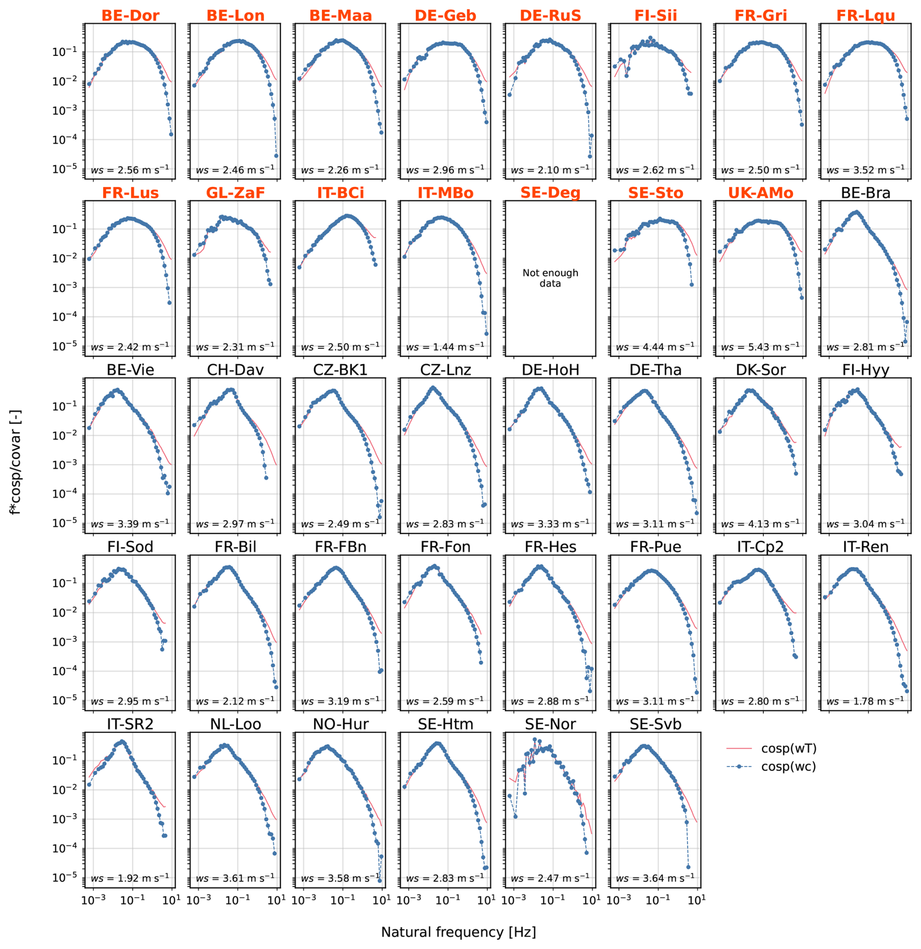
Figure B1 Average normalised co-spectra of sensible heat (wT, red) and CO₂ flux (wc, blue). co-spectra are normalised by their respective covariances. For each site, data from the median WS class is used and the mean WS value of that class shown. The co-spectra shown have been filtered using the quality thresholds defined for the cof computation, and they represent the data directly used to derive the TF and subsequently the cof. In practice, this filtering retains only high-quality data characterised by strong turbulent fluxes. The red bold titles represent the low-measurement-height sites.

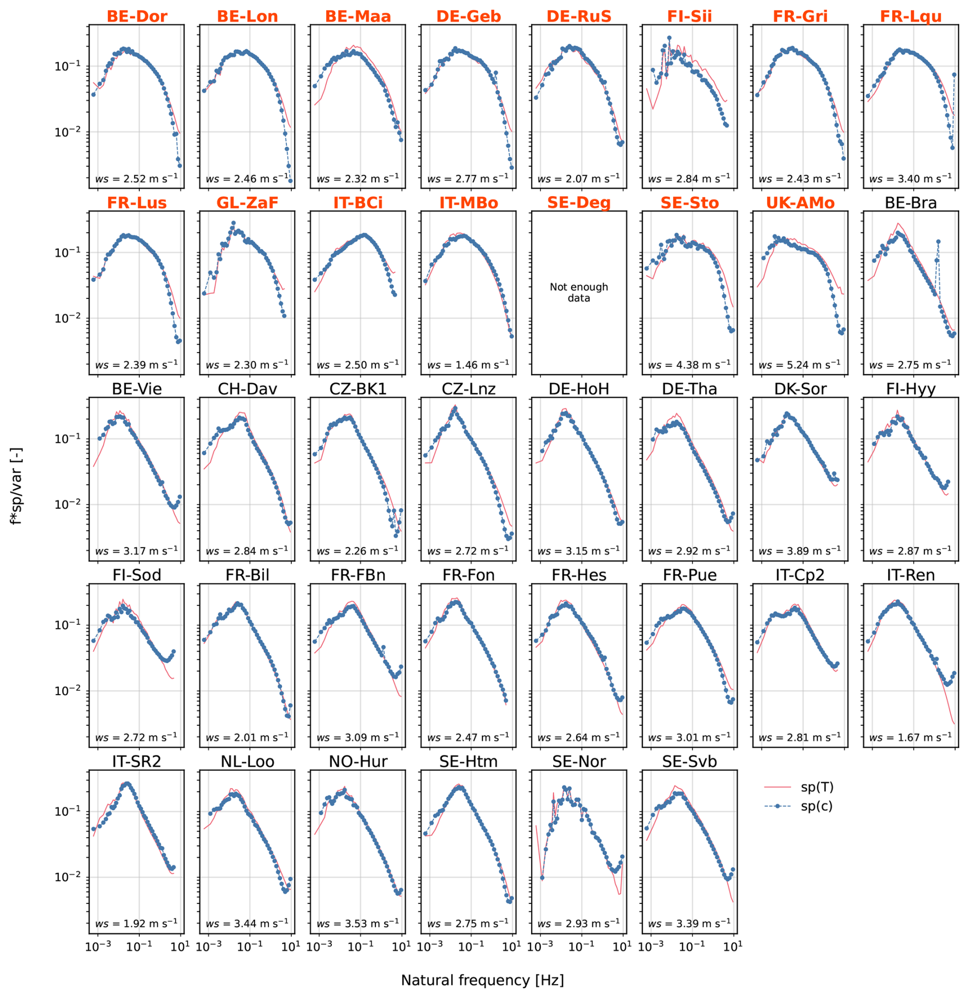
Figure B2 Average normalised spectra of sonic temperature (T, red) and CO₂ mixing ratio (c, blue). Spectra are normalised by their respective variances. For each site, data from the median wind speed class is used and the mean value of that class shown. The spectra shown have been filtered using the quality thresholds defined for the cof computation, and they represent the data used to derive the TF and subsequently the cof. In practice, this filtering retains only high-quality data characterised by strong turbulent fluxes. The red bold titles represent the low-measurement-height sites.

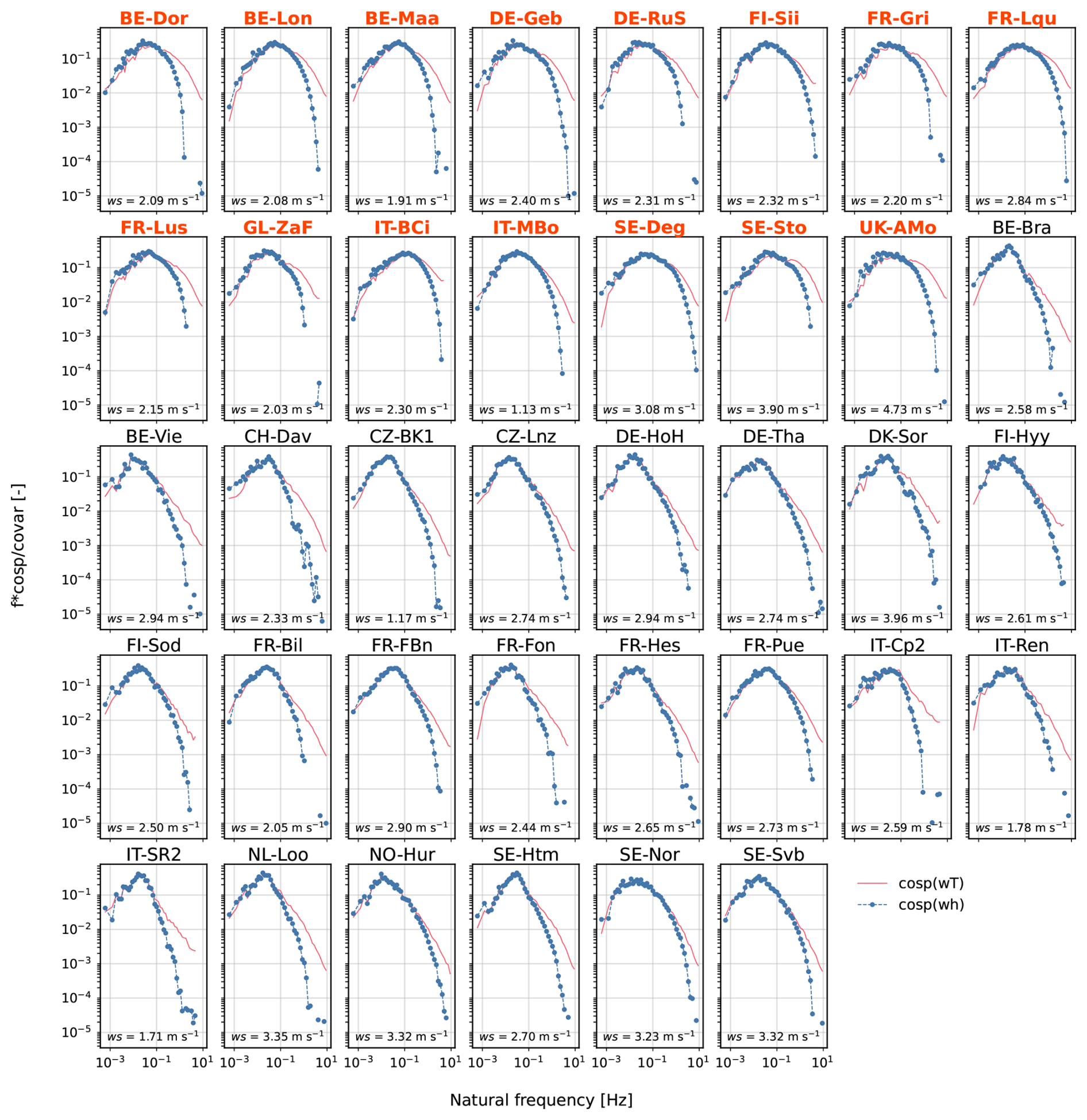
Figure B3 Same as Fig. B1, but for H₂O. The median RH class is selected, in addition to the median WS class.

Figure B4 Same as Fig. B2, but for H₂O. The median RH class is selected, in addition to the median WS class.

Appendix C: Cumulated fluxes

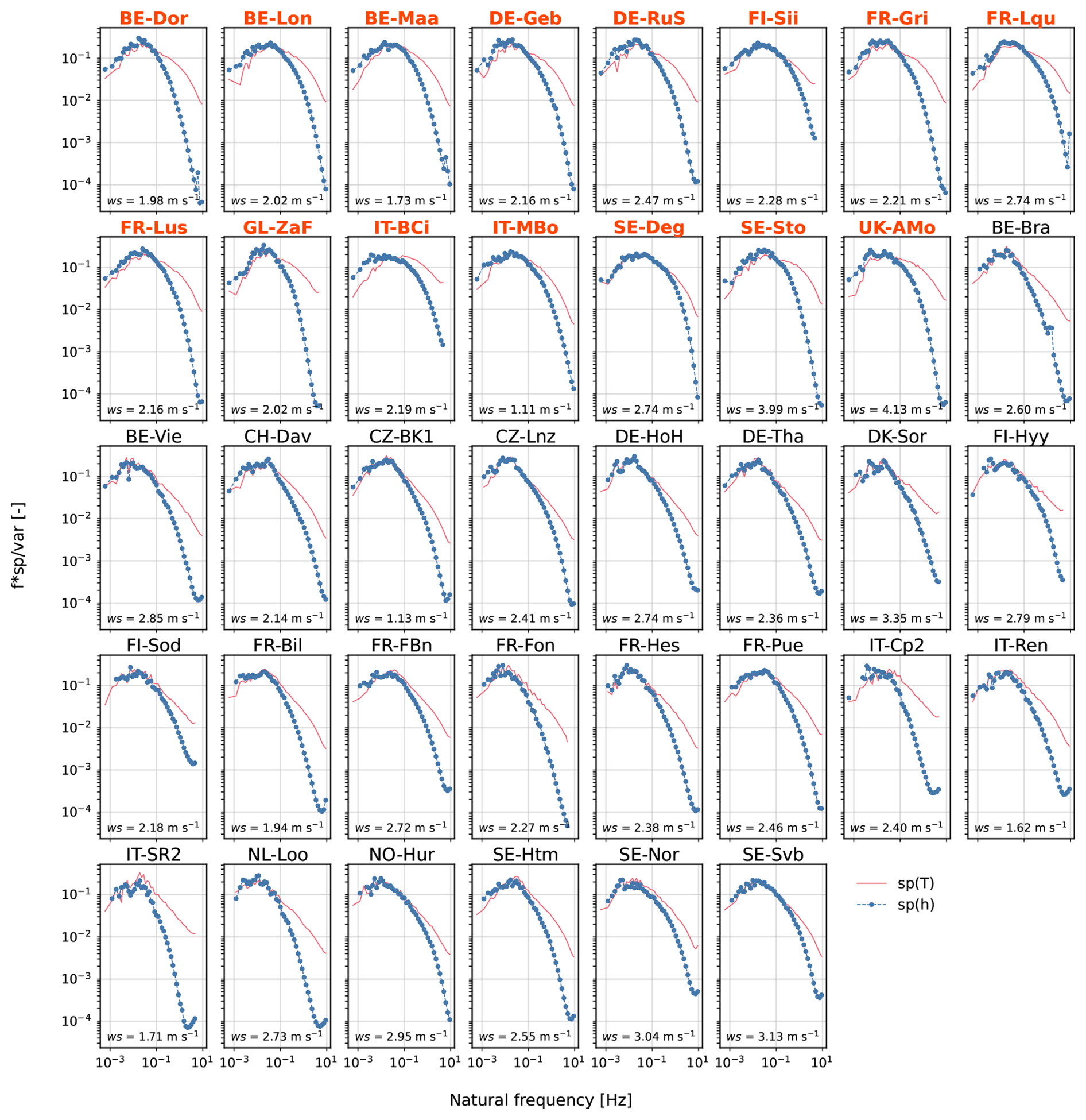
The yearly cumulative fluxes for CO₂ and H₂O are presented in Figs. C1 and C2. The half-hourly fluxes used for the cumulative flux computation were filtered for poor quality and low atmospheric turbulence and filtered time series were not gap-filled to avoid additional complexity. Therefore, the cumulative values are not intended to represent the true yearly exchange, but relative differences between methods are supposed to be representative. The mean data coverage after filtering was 39 % for both CO₂ and H₂O. It should be noted that for water fluxes, as half-hours with low u^* mainly include night-time periods during which fluxes are generally very small, their addition would not change much the overall budget, so that the presented cumulative value can be considered as a fairly good estimate of the true LE budget over the year.

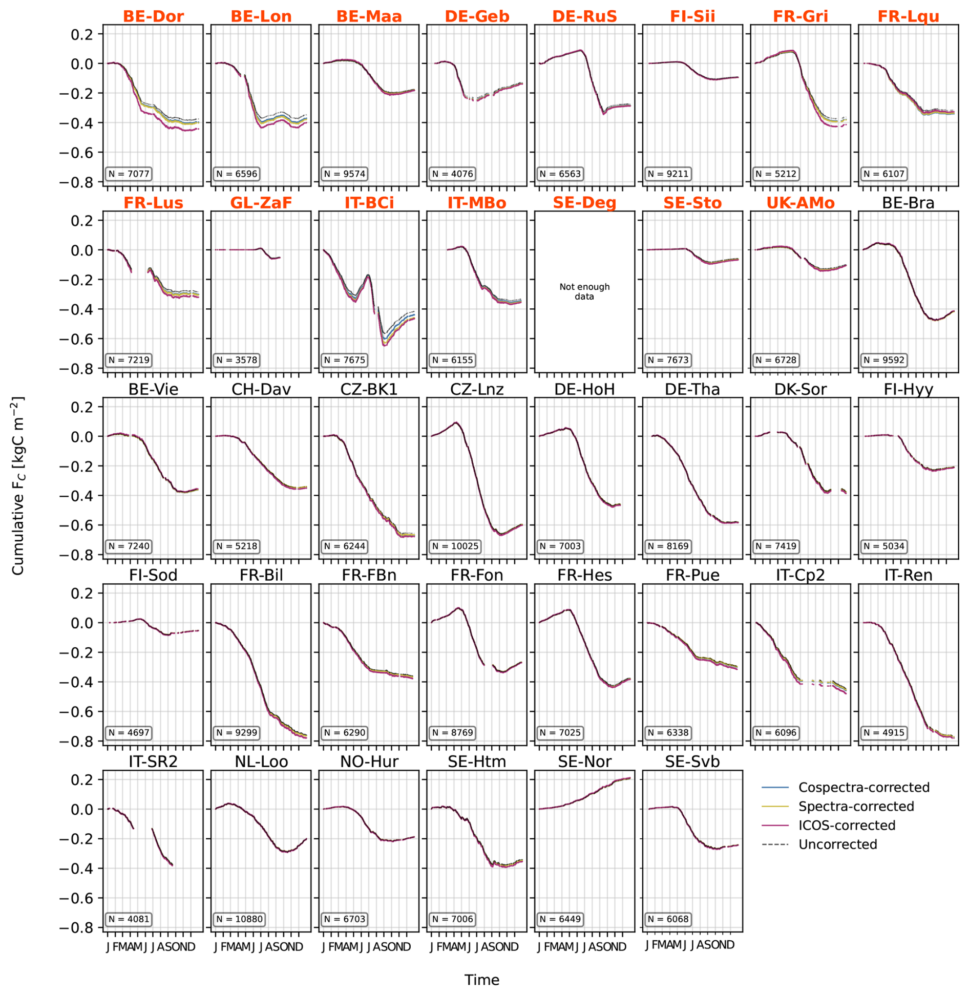
Figure C1 CO₂ cumulative fluxes for quality and u^* filtered data only. Uncorrected fluxes, spectra-, co-spectra- and ICOS-corrected fluxes are shown. N is the number of half-hours used. The storage term is not included (only turbulent data is used). The red bold titles represent the low-measurement-height sites.

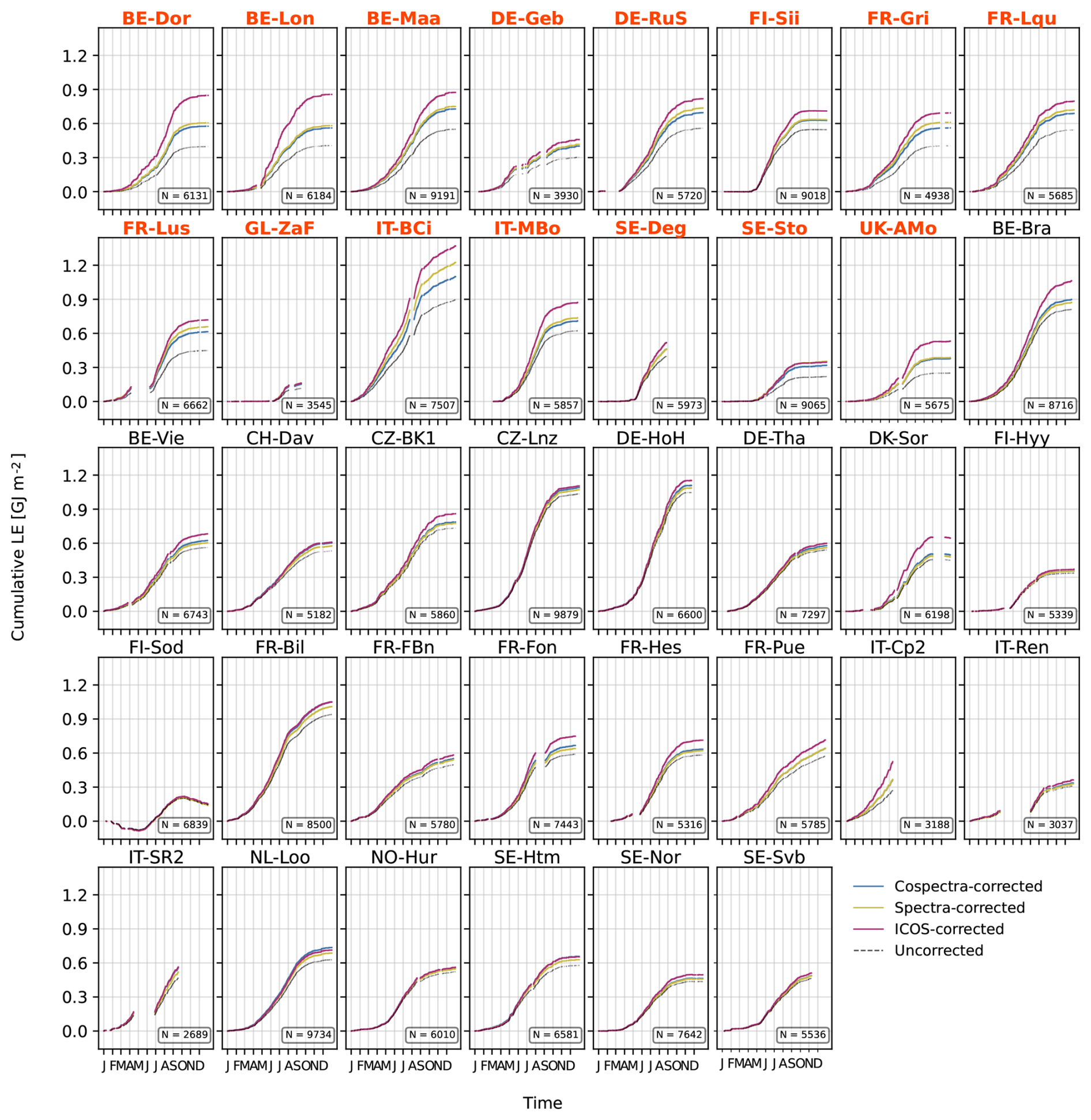
Figure C2 LE cumulative fluxes for quality and u^* filtered data. Uncorrected fluxes, spectra-, co-spectra- and ICOS-corrected fluxes are shown. N is the number of half-hours used. The red bold titles represent the low-measurement-height sites.

Appendix D: H₂O correction dependence on relative humidity

The spectral analysis and correction procedure was built to account for the known dependence of water spectral losses to RH. Therefore, each site's full dataset is divided into RH classes prior to both cof and CF computation. The results of such classification are investigated. The cof is expected to decrease with  RH following an exponential decay, which is found to be the case for all sites (Fig. D1). The cof–RH dependence has a direct consequence on the CF computation, which is found to be driven by both WS and RH (Figs. D2 and D3).

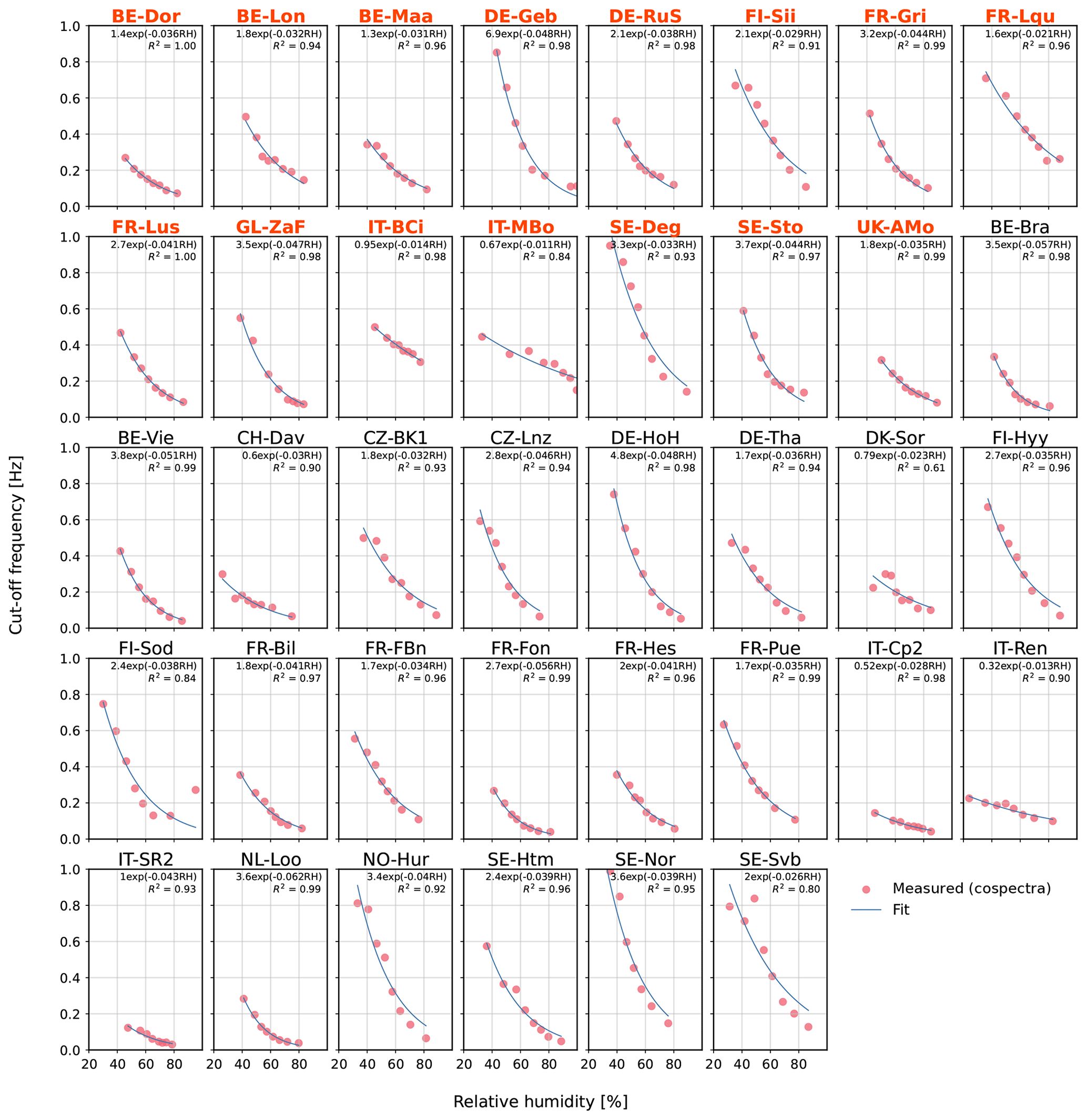
Figure D1 Fit of exponential equation to the average cof values per RH class The red bold titles represent the low-measurement-height sites.

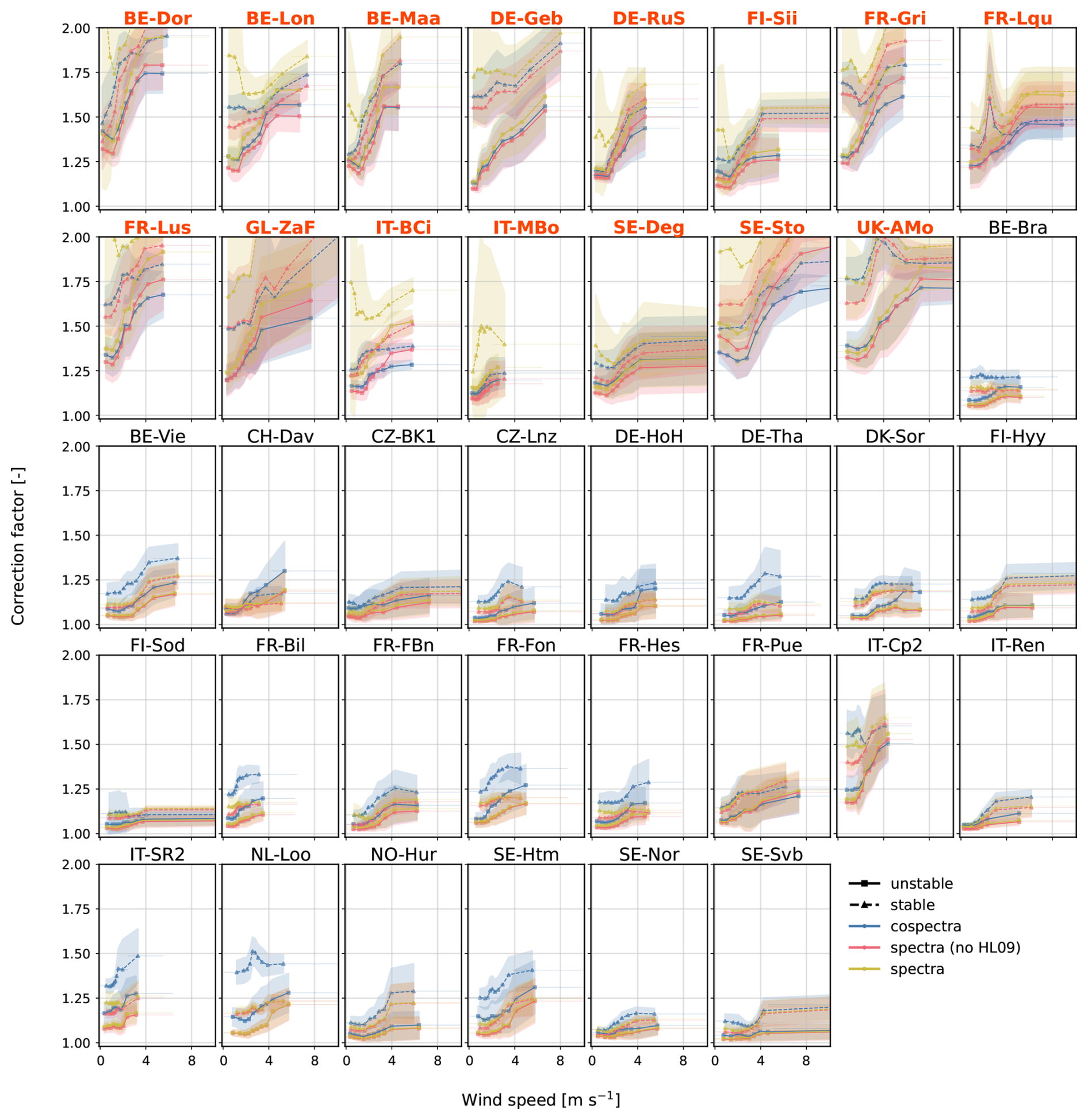
Figure D2 Spectral and co-spectral H₂O CF as a function of wind speed, as shown in Fig. 8 but for all relative humidity conditions. The additional dependence on RH is found in the larger data spread (shaded area around the lines corresponding to ±1 SD around the mean). The red bold titles represent the low-measurement-height sites.

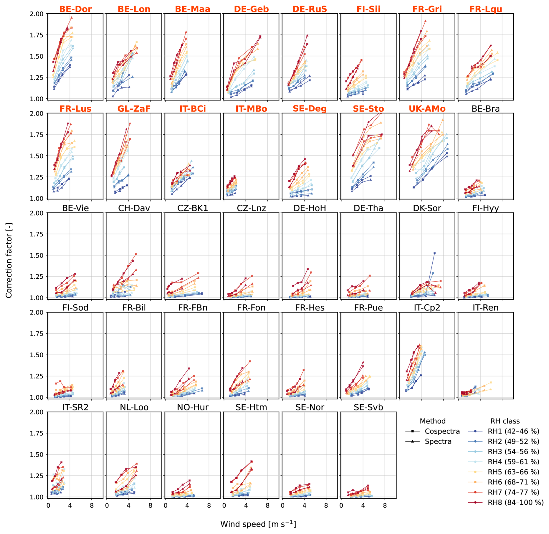
Figure D3 Dependence of H₂O CF on wind speed and relative humidity classes for unstable conditions only. The RH are built as constant-point classes based on the available data, and they are therefore slightly different for each site. The spectral results (triangles) are fully experimental CF, prior to the inclusion of the sensor separation term. The red bold titles represent the low-measurement-height sites.

Appendix E: Theoretical dependencies of the sensor separation correction factor

The experimental part of the spectral correction approach does not include the attenuation from the sensor separation effect, which therefore has to be accounted for with an additional theoretical term (Eq. 6). In this work, the sensor separation CF defined by Horst and Lenschow (2009) is used (Eqs. 16 and 28, corresponding to the cross-wind and vertical separation effects respectively). Their method uses an exponential model to estimate the attenuation as a function of co-spectral peak frequency (parametrised according to stability) and the distance between the sensors (depending on wind direction). The shapes of these relationships and the corresponding CF orders of magnitude are shown for artificial data in Fig. E1, and will be tested against experimental data.

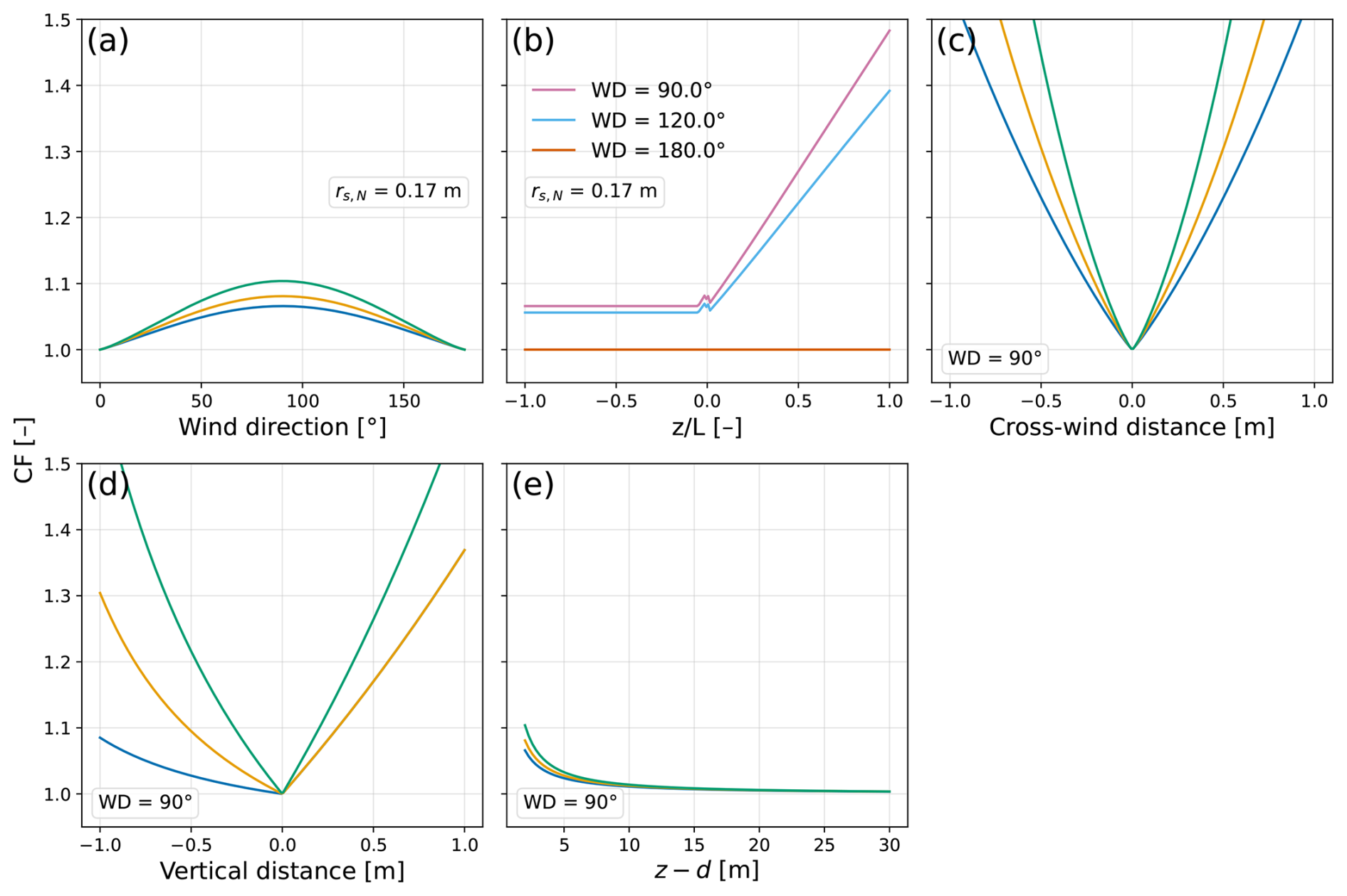
Figure E1 Analytical dependencies of sensor separation correction factor according to Horst and Lenschow (2009). Cross-separation wind direction (90° in the figure) yields the maximum distance between the sensors and thus the maximum CF (a). The CF is highly sensitive to stability for $\frac{z}{L}$ > 0 (b). A strong dependence on horizontal (c) and vertical (d) distances between the sensors is expected. Finally, sites measuring closer to the canopy are linked to higher CFs.

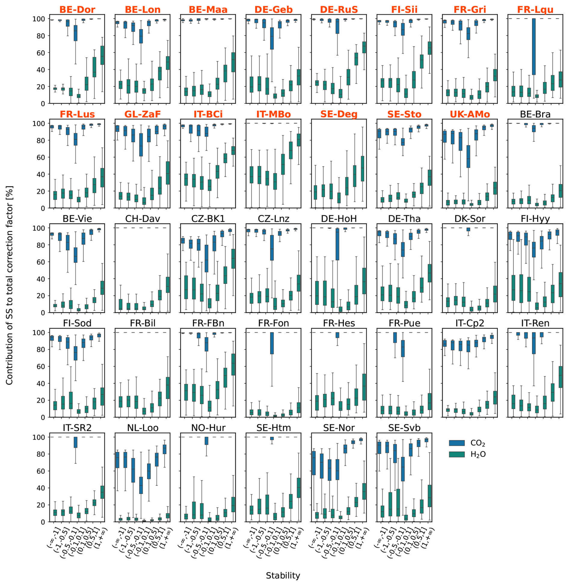
Figure E2 Contribution of sensor separation term to overall correction factor, for both CO₂ and H₂O, by stability condition. The percentage change is computed as $\mathrm{100}\times ({\text{CF}}_{\text{HL09}}-\mathrm{1})/(\text{CF}-\mathrm{1})$. Box frame = 25–75 % interquartile range (IQR), bold line = median, whiskers = 1.5 × IQR. The red bold titles represent the low-measurement-height sites.

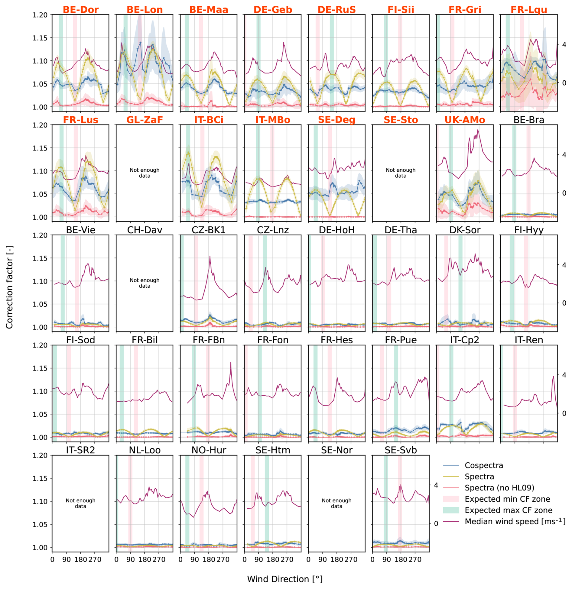
Figure E3 CO₂ co-spectral and spectral correction factors as a function of wind direction, grouped in equal-number-of-points bins. Data is filtered for unstable conditions. The direction effect of wind speed is visible on the dependence of the CFs on WD. The red bold titles represent the low-measurement-height sites.

Appendix F: Flux-tower stations used

Table F1 Site and set-up characteristics.

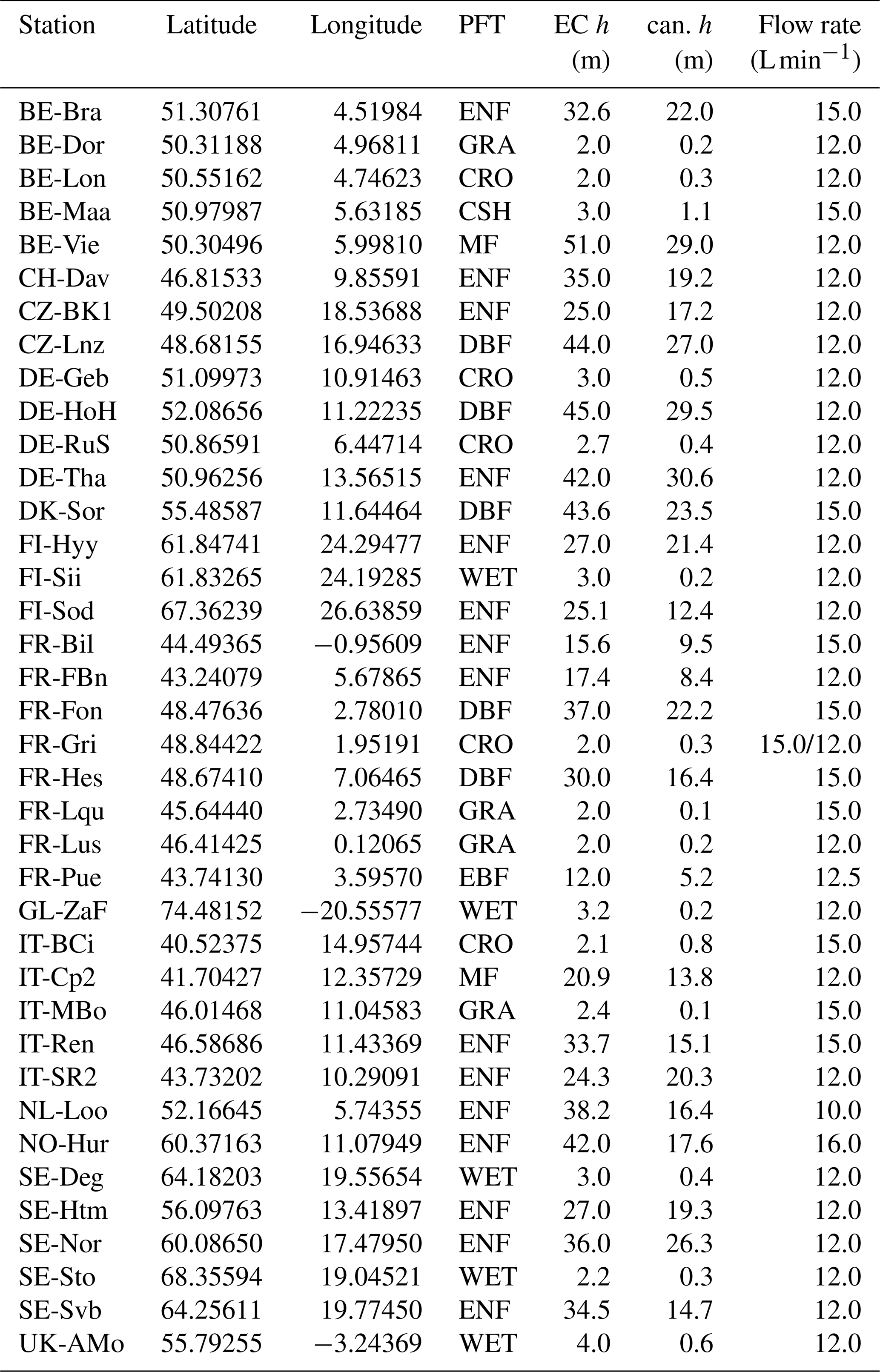
Note: in addition to station official ID, coordinates are reported, together with plant functional type (PFT), height of the eddy covariance system (EC h, m), mean canopy height (can h, m), and flow rate of the gas sampling system (L min⁻¹). PFT acronyms: CRO, Croplands; CSH, Closed Shrublands; DBF, Deciduous Broadleaf Forests; EBF, Evergreen Broadleaf Forests; ENF, Evergreen Needleleaf Forests; GRA, Grasslands; MF, Mixed Forests; WET, Permanent Wetlands.