A neural network approach to estimating a posteriori distributions of Bayesian retrieval problems

A neural-network-based method, quantile regression neural networks (QRNNs), is proposed as a novel approach to estimating the a posteriori distribution of Bayesian remote sensing retrievals. The advantage of QRNNs over conventional neural network retrievals is that they learn to predict not only a single retrieval value but also the associated, case-specific uncertainties. In this study, the retrieval performance of QRNNs is characterized and compared to that of other state-of-the-art retrieval methods. A synthetic retrieval scenario is presented and used as a validation case for the application of QRNNs to Bayesian retrieval problems. The QRNN retrieval performance is evaluated against Markov chain Monte Carlo simulation and another Bayesian method based on Monte Carlo integration over a retrieval database. The scenario is also used to investigate how different hyperparameter configurations and training set sizes affect the retrieval performance. In the second part of the study, QRNNs are applied to the retrieval of cloud top pressure from observations by the Moderate Resolution Imaging Spectroradiometer (MODIS). It is shown that QRNNs are not only capable of achieving similar accuracy to standard neural network retrievals but also provide statistically consistent uncertainty estimates for non-Gaussian retrieval errors. The results presented in this work show that QRNNs are able to combine the flexibility and computational efficiency of the machine learning approach with the theoretically sound handling of uncertainties of the Bayesian framework. Together with this article, a Python implementation of QRNNs is released through a public repository to make the method available to the scientific community.

1 Introduction

The retrieval of atmospheric quantities from remote sensing measurements constitutes an inverse problem that generally does not admit a unique, exact solution. Measurement and modeling errors, as well as limited sensitivity of the observation system, preclude the assignment of a single, discrete solution to a given observation. A meaningful retrieval should thus consist of a retrieved value and an estimate of uncertainty describing a range of values that are likely to produce a measurement similar to the one observed. However, even if a retrieval method allows for explicit modeling of retrieval uncertainties, their computation and representation are often possible only in an approximate manner.

The Bayesian framework provides a formal way of handling the ill-posedness of the retrieval problem and its associated uncertainties. In the Bayesian formulation (Rodgers, 2000), the solution of the inverse problem is given by the a posteriori distribution p(x|y), i.e., the conditional distribution of the retrieval quantity x given the observation y. Under the modeling assumptions, the posterior distribution represents all available knowledge about the retrieval quantity x after the measurement, accounting for all considered retrieval uncertainties. Bayes' theorem states that the a posteriori distribution is proportional to the product p(y|x)p(x) of the a priori distribution p(x) and the conditional probability of the observed measurement p(y|x). The a priori distribution p(x) represents knowledge about the quantity x that is available before the measurement and can be used to aid the retrieval with supplementary information.

For a given retrieval, the a posteriori distribution can generally not be expressed in closed form, and different methods have been developed to compute approximations to it. In cases that allow a sufficiently precise and efficient simulation of the measurement, a forward model can be used to guide the solution of the inverse problem. If such a forward model is available, the most general technique to compute the a posteriori distribution is Markov chain Monte Carlo (MCMC) simulation. MCMC denotes a set of methods that iteratively generate a sequence of samples, whose sampling distribution approximates the true a posteriori distribution. MCMC simulations have the advantage of allowing the estimation of the a posteriori distribution without requiring any simplifying assumptions on a priori knowledge, measurement error or the forward model. The disadvantage of MCMC simulation is that each retrieval requires a high number of forward-model evaluations, which in many cases makes the method computationally too demanding to be practical. For remote sensing retrievals, the method is therefore of interest rather for testing and validation (Tamminen and Kyrölä, 2001), such as in the retrieval algorithm developed by Evans et al. (2012).

A method that avoids costly forward-model evaluations during the retrieval has been proposed by Kummerow et al. (1996). The method is based on Monte Carlo integration of importance-weighted samples in a retrieval database $\mathit{\left\{}\right({\mathit{y}}_i,x_i){\mathit{\}}}_{i=\mathrm{0}}^n$, which consists of pairs of observations y_i and corresponding values x_i of the retrieval quantity. The method will be referred to in the following as Bayesian Monte Carlo integration (BMCI). Even though the method is less computationally demanding than methods involving forward-model calculations during the retrieval, it may require the traversal of a potentially large retrieval database. Furthermore, the incorporation of ancillary data to aid the retrieval requires careful stratification of the retrieval database, as it is performed in the Goddard profiling algorithm (Kummerow et al., 2015) for the retrieval of precipitation profiles. Further applications of the method can be found for example in the work by Rydberg et al. (2009) or Evans et al. (2012).

The optimal estimation method (Rodgers, 2000), in short OEM (also 1D-Var, for one-dimensional variational retrieval), simplifies the Bayesian retrieval problem assuming that a priori knowledge and measurement uncertainty both follow Gaussian distributions and that the forward model is only moderately nonlinear. Under these assumptions, the a posteriori distribution is approximately Gaussian. The retrieved values in this case are the mean and maximum of the a posteriori distribution, which coincide for a Gaussian distribution, together with the covariance matrix describing the width of the a posteriori distribution. In cases where an efficient forward model for the computation of simulated measurements and corresponding Jacobians is available, the OEM has become the quasi-standard method for Bayesian retrievals. Nonetheless, even neglecting the validity of the assumptions of Gaussian a priori and measurement errors as well as linearity of the forward model, the method is unsuitable for retrievals that involve complex radiative processes. In particular, since the OEM requires the computation of the Jacobian of the forward model, processes such as surface or cloud scattering become too expensive to model online during the retrieval.

Compared to the Bayesian retrieval methods discussed above, machine learning provides a more flexible approach to learning computationally efficient retrieval mappings directly from data. Large amounts of data available from simulations, collocated observations or in situ measurements, as well as increasing computational power to speed up the training, have made machine learning techniques an attractive alternative to approaches based on (Bayesian) inverse modeling. Numerous applications of machine learning regression methods to retrieval problems can be found in the recent literature (Brath et al., 2018; Holl et al., 2014; Håkansson et al., 2018; Jiménez et al., 2003; Strandgren et al., 2017; Wang et al., 2017). All of these examples, however, neglect the probabilistic character of the inverse problem and provide only a scalar estimate of the retrieval. Uncertainty estimates in these retrievals are provided in the form of mean errors computed on independent test data, which is a clear drawback compared to Bayesian methods. A notable exception is the work by Aires et al. (2004), which applies the Bayesian framework to estimate errors in the retrieved quantities due to uncertainties on the learned neural network parameters. However, the only difference to the approaches listed above is that the retrieval errors, estimated from the error covariance matrix observed on the training data, are corrected for uncertainties in the network parameters. With respect to the intrinsic retrieval uncertainties, the approach is thus afflicted with the same limitations. Furthermore, the complexity of the required numerical operations makes it suitable only for small training sets and simple networks.

In this article, quantile regression neural networks (QRNNs) are proposed as a method to use neural networks to estimate the a posteriori distribution of remote sensing retrievals. Originally proposed by Koenker and Bassett Jr. (1978), quantile regression is a method for fitting statistical models to quantile functions of conditional probability distributions. Applications of quantile regression using neural networks (Cannon, 2011) and other machine learning methods (Meinshausen, 2006) exist, but to the best knowledge of the authors this is the first application of QRNNs to remote sensing retrievals. The aim of this work is to combine the flexibility and computational efficiency of the machine learning approach with the theoretically sound handling of uncertainties in the Bayesian framework.

A formal description of QRNNs and the retrieval methods against which they will be evaluated is provided in Sect. 2. A simulated retrieval scenario is used to validate the approach against BMCI and MCMC in Sect. 3. Section 4 presents the application of QRNNs to the retrieval of cloud top pressure and associated uncertainties from satellite observations in the visible and infrared. Finally, the conclusions from this work are presented in Sect. 5.

2 Methods

This section introduces the Bayesian retrieval formulation and the retrieval methods used in the subsequent experiments. Two Bayesian methods, Markov chain Monte Carlo simulation and Bayesian Monte Carlo integration, are presented. Quantile regression neural networks are introduced as a machine learning approach to estimating the a posteriori distribution of Bayesian retrieval problems. The section closes with a discussion of the statistical metrics that are used to compare the methods.

2.1 The retrieval problem

The general problem considered here is the retrieval of a scalar quantity x∈R from an indirect measurement given in the form of an observation vector y∈R^m. In the Bayesian framework, the retrieval problem is formulated as finding the posterior distribution p(x|y) of the quantity x given the measurement y. Formally, this solution can be obtained by application of Bayes' theorem:

$$\begin{array}{}\text{(1)}& p\left(x\right|\mathit{y})={\displaystyle \frac{p\left(\mathit{y}\right|x\left)p\right(x)}{\int p(x^{\prime },\mathit{y})\mathrm{d}{x}^{\prime }}}.\end{array}$$

The a priori distribution p(x) represents the knowledge about the quantity x that is available prior to the measurement. The a priori knowledge introduced into the retrieval formulation regularizes the ill-posed inverse problem and ensures that the retrieval solution is physically meaningful. The a posteriori distribution of a scalar retrieval quantity x can be represented by the corresponding cumulative distribution function (CDF) F_x|y(x), which is defined as

$$\begin{array}{}\text{(2)}& F_{x|\mathit{y}}\left(x\right)=\underset{-\mathrm{\infty }}{\overset{x}{\int }}p\left(x^{\prime }\right|\mathit{y})\mathrm{d}{x}^{\prime }.\end{array}$$

2.2 Bayesian retrieval methods

Bayesian retrieval methods are methods that use the expression for the a posteriori distribution in Eq. (1) to compute a solution to the retrieval problem. Since the a posteriori distribution can generally not be computed or sampled directly, these methods approximate the posterior distribution to varying degrees of accuracy.

2.2.1 Markov chain Monte Carlo

MCMC simulation denotes a set of methods for the generation of samples from arbitrary posterior distributions p(x|y). The general principle is to compute samples from an approximate distribution and refine them in a way such that their distribution converges to the true a posteriori distribution (Gelman et al., 2013). In this study, the Metropolis algorithm is used to implement MCMC. The Metropolis algorithm iteratively generates a sequence of states ${\mathit{x}}_{\mathrm{0}},{\mathit{x}}_{\mathrm{1}},\mathrm{\dots }$ using a symmetric proposal distribution $J_t\left({\mathit{x}}^{*}\right|{\mathit{x}}_{t-\mathrm{1}})$. In each step of the algorithm, a proposal x^* for the next step is generated by sampling from $J_t\left({\mathit{x}}^{*}\right|{\mathit{x}}_{t-\mathrm{1}})$. The proposed state x^* is accepted as the next simulation step x_t with probability $\text{min}\left\{\mathrm{1},\frac{p\left({\mathit{x}}^{*}\right|\mathit{y})}{p\left({\mathit{x}}_{t-\mathrm{1}}\right|\mathit{y})}\right\}$. Otherwise x^* is rejected and the current simulation step x_t−1 is kept for x_t. If the proposal distribution $J({\mathit{x}}^{*},{\mathit{x}}_{t-\mathrm{1}})$ is symmetric and samples generated from it satisfy the Markov chain property with a unique stationary distribution, the Metropolis algorithm is guaranteed to produce a distribution of samples which converges to the true a posteriori distribution.

2.2.2 Bayesian Monte Carlo integration

The BMCI method is based on the use of importance sampling to approximate integrals over the a posteriori distribution of a given retrieval case. Consider an integral of the form

$$\begin{array}{}\text{(3)}& \int f\left(x^{\prime }\right)p\left(x^{\prime }\right|\mathit{y})\mathrm{d}{x}^{\prime }.\end{array}$$

Applying Bayes' theorem, the integral can be written as

$$\int f\left(x^{\prime }\right)p\left(x^{\prime }\right|\mathit{y})\mathrm{d}{x}^{\prime }=\int f(x^{\prime }){\displaystyle \frac{p\left(\mathit{y}\right|x^{\prime }\left)p\right(x^{\prime })}{\int p\left(\mathit{y}\right|x^{\prime \prime })\mathrm{d}{x}^{\prime \prime }}}\mathrm{d}{x}^{\prime }.$$

The last integral can be approximated by a sum over an observation database $\mathit{\left\{}\right({\mathit{y}}_i,x_i){\mathit{\}}}_{i=\mathrm{1}}^n$ that is distributed according to the a priori distribution p(x):

$$\int f\left(x^{\prime }\right)p\left(x^{\prime }\right|\mathit{y})\mathrm{d}{x}^{\prime }\approx {\displaystyle \frac{\mathrm{1}}{C}}\sum _{i=\mathrm{1}}^n{w}_i(\mathit{y}\left)f\right(x_i),$$

with the normalization factor C given by $C={\sum }_{i=\mathrm{1}}^n{w}_i\left(\mathit{y}\right).$ The weights w_i(y) are given by the probability p(y|y_i) of the observed measurement y conditional on the database measurement y_i, which is usually assumed to be multivariate Gaussian with covariance matrix S_o:

$$w_i\left(\mathit{y}\right)\propto \exp \left\{-{\displaystyle \frac{(\mathit{y}-{\mathit{y}}_i{)}^T{\mathbf{S}}_o^{-\mathrm{1}}(\mathit{y}-{\mathit{y}}_i)}{\mathrm{2}}}\right\}.$$

By approximating integrals of Eq. (3), it is possible to estimate the expectation value and variance of the a posteriori distribution by choosing f(x)=x and $f\left(x\right)=(x-\mathcal{E}(x\left|\mathit{y}\right){)}^{\mathrm{2}}$, respectively. While this is suitable to represent Gaussian distributions, a more general representation of the a posteriori distribution can be obtained by estimating the corresponding CDF (cf. Eq. 2) using

$$\begin{array}{}\text{(4)}& F_{x|\mathit{y}}\left(x\right)\approx {\displaystyle \frac{\mathrm{1}}{C}}\sum _{x_i<x}{w}_i\left(\mathit{y}\right).\end{array}$$

2.3 Machine learning

Neglecting uncertainties, the retrieval of a quantity x from a measurement vector y may be viewed as a simple multiple regression task. In machine learning, regression problems are typically approached by training a parametrized model $f:\mathit{x}\mapsto \mathit{y}$ to predict a desired output y from given input x. Unfortunately, the use of the variables x and y in machine learning is directly opposite to their use in inverse theory. For the remainder of this section the variables x and y will be used to denote, respectively, the input and output to the machine learning model to ensure consistency with the common notation in the field of machine learning. The reader must keep in mind that the method is applied in the later sections to predict a retrieval quantity x from a measurement y.

2.3.1 Supervised learning and loss functions

Machine learning regression models are trained using supervised training, in which the model f learns the regression mapping from a training set $\mathit{\{}{\mathit{x}}_i,{\mathit{y}}_i{\mathit{\}}}_{i=\mathrm{1}}^n$ with input values x_i and expected output values y_i. The training is performed by finding model parameters that minimize the mean of a given loss function ℒ(f(x),y) on the training set. The most common loss function for regression tasks is the squared error loss

$$\begin{array}{}\text{(5)}& {\mathcal{L}}_{\mathrm{se}}\left(f\right(\mathit{x}),\mathit{y})=\left(f\right(\mathit{x})-\mathit{y}{)}^T(f\left(\mathit{x}\right)-\mathit{y}),\end{array}$$

which trains the model f to minimize the mean squared distance of the neural network prediction f(x) from the expected output y on the training set. If the estimand y is a random vector drawn from a conditional probability distribution p(y|x), a regressor trained using a squared error loss function learns to predict the conditional expectation value of the distribution p(y|x) (Bishop, 2006). Depending on the choice of the loss function, the regressor can also learn to predict other statistics of the distribution p(y|x) from the training data.

2.3.2 Quantile regression

Given the cumulative distribution function F(x) of a probability distribution p, its τth quantile x_τ is defined as

$$\begin{array}{}\text{(6)}& {\displaystyle }{x}_{\mathit{\tau }}{\displaystyle }=inf\mathit{\{}x:F(x)\ge \mathit{\tau }\mathit{\}},\end{array}$$

i.e., the greatest lower bound of all values of x for which F(x)≥τ. As shown by Koenker (2005), the τth quantile x_τ of F minimizes the expectation value ${\mathcal{E}}_x\left({\mathcal{L}}_{\mathit{\tau }}(x_{\mathit{\tau }},x)\right)={\int }_{-\mathrm{\infty }}^{\mathrm{\infty }}{\mathcal{L}}_{\mathit{\tau }}(x_{\mathit{\tau }},x^{\prime })p\left(x^{\prime }\right)\mathrm{d}{x}^{\prime }$ of the function

$$\begin{array}{}\text{(7)}& {\displaystyle }{\mathcal{L}}_{\mathit{\tau }}(x_{\mathit{\tau }},x){\displaystyle }=\left\{\begin{array}{ll}\mathit{\tau }|x-x_{\mathit{\tau }}|,& x_{\mathit{\tau }}<x\\ (\mathrm{1}-\mathit{\tau })|x-x_{\mathit{\tau }}|,& \text{otherwise}.\end{array}\right.\end{array}$$

By training a machine learning regressor f to minimize the mean of the quantile loss function ℒ_τ(f(x),y) over a training set $\mathit{\{}{\mathit{x}}_i,y_i{\mathit{\}}}_{i=\mathrm{1}}^n$, the regressor learns to predict the quantiles of the conditional distribution p(y|x). This can be extended to obtain an approximation of the cumulative distribution function of F_y|x(y) by training the network to estimate multiple quantiles of p(y|x).

2.3.3 Neural networks

A neural network computes a vector of output activations y from a vector of input activations x. Feed-forward artificial neural networks (ANNs) compute the vector y by application of a given number of subsequent, learnable transformations to the input activations x:

$$\begin{array}{ll}{\displaystyle }{\mathit{x}}_{\mathrm{0}}& {\displaystyle }=\mathit{x},\\ {\displaystyle }{\mathit{x}}_i& {\displaystyle }=f_i\left({\mathbf{W}}_i{\mathit{x}}_{i-\mathrm{1}}+{\mathit{\theta }}_i\right),\\ {\displaystyle }\mathit{y}& {\displaystyle }={\mathit{x}}_n.\end{array}$$

The activation functions f_i as well as the number and sizes of the hidden layers ${\mathit{x}}_{\mathrm{1}},\mathrm{\dots },{\mathit{x}}_{n-\mathrm{1}}$ are prescribed, structural parameters of a neural network model, generally referred to as hyperparameters. The learnable parameters of the model are the weight matrices W_i and bias vectors θ_i of each layer. Neural networks can be efficiently trained in a supervised manner by using gradient-based minimization methods to find suitable weights W_i and bias vectors θ_i. By using the mean of the quantile loss function ℒ_τ as the training criterion, a neural network can be trained to predict the quantiles of the distribution p(y|x), thus turning the network into a quantile regression neural network.

2.3.4 Adversarial training

Adversarial training is a data augmentation technique that has been proposed to increase the robustness of neural networks to perturbations in the input data (Goodfellow et al., 2014). It has been shown to be effective also as a method to improve the calibration of probabilistic predictions from neural networks (Lakshminarayanan et al., 2016). The basic principle of adversarial training is to augment the training data with perturbed samples that are likely to yield a large change in the network prediction. The method used here to implement adversarial training is the fast gradient sign method proposed by Goodfellow et al. (2014). For a training sample (x_i,y_i) consisting of input x_i∈Rⁿ and expected output y_i∈R^m, the corresponding adversarial sample $({\stackrel{\mathrm{̃}}{\mathit{x}}}_i,{\mathit{y}}_i)$ is chosen to be

$$\begin{array}{}\text{(8)}& {\displaystyle }{\stackrel{\mathrm{̃}}{\mathit{x}}}_i={\mathit{x}}_i+{\mathit{\delta }}_{\text{adv}}\cdot \text{sign}\left({\displaystyle \frac{\mathrm{d}\mathcal{L}\left(f\right({\mathit{x}}_i),{\mathit{y}}_i)}{\mathrm{d}{\mathit{x}}_i}}\right);\end{array}$$

i.e., the direction of the perturbation is chosen in such a way that it maximizes the absolute change in the loss function ℒ due to an infinitesimal change in the input parameters. The adversarial perturbation factor δ_adv determines the strength of the perturbation and becomes an additional hyperparameter of the neural network model.

2.4 Evaluating probabilistic predictions

A problem that remains is how to compare two estimates $p^{\prime }\left(x\right|\mathit{y}),p^{\prime \prime }(x\left|\mathit{y}\right)$ of a given a posteriori distribution against a single observed sample x from the true distribution p(x|y). A good probabilistic prediction for the value x should be sharp, i.e., concentrated in the vicinity of x, but at the same time well calibrated, i.e., predicting probabilities that truthfully reflect observed frequencies (Gneiting et al., 2005). Summary measures for the evaluation of predicted conditional distributions are called scoring rules (Gneiting and Raftery, 2007). An important property of scoring rules is propriety, which formalizes the concept of the scoring rule rewarding both sharpness and calibration of the prediction. Besides providing reliable measures for the comparison of probabilistic predictions, proper scoring rules can be used as loss functions in supervised learning to incentivize statistically consistent predictions.

The quantile loss function given in Eq. (7) is a proper scoring rule for quantile estimation and can thus be used to compare the skill of different methods for quantile estimation (Gneiting and Raftery, 2007). Another proper scoring rule for the evaluation of an estimated cumulative distribution function F against an observed value x is the continuous ranked probability score (CRPS):

$$\begin{array}{}\text{(9)}& {\displaystyle }\text{CRPS}(F,x){\displaystyle }=\underset{-\mathrm{\infty }}{\overset{\mathrm{\infty }}{\int }}{\left(F\left(x^{\prime }\right)-I_{x\le x^{\prime }}\right)}^{\mathrm{2}}\mathrm{d}{x}^{\prime }.\end{array}$$

Here, $I_{x\le x^{\prime }}$ is the indicator function that is equal to 1 when the condition $x\le x^{\prime }$ is true and 0 otherwise. For the methods used in this article the integral can only be evaluated approximately. The exact way in which this is done for each method is described in detail in Sect. 3.1.3 and 3.1.4.

The scoring rules presented above evaluate probabilistic predictions against a single observed value. However, since MCMC simulations can be used to approximate the true a posteriori distribution to an arbitrary degree of accuracy, the probabilistic predictions obtained from BMCI and QRNN can be compared directly to the a posteriori distributions obtained using MCMC. In the idealized case where the modeling assumptions underlying the MCMC simulations are true, the sampling distribution obtained from MCMC will converge to the true posterior and can be used as a ground truth to assess the predictions obtained from the other methods.

2.4.1 Calibration plots

Calibration plots are a graphical method for assessing the calibration of prediction intervals derived from probabilistic predictions. For a set of prediction intervals with probabilities $p=p_{\mathrm{1}},\mathrm{\dots },p_n$, the fraction of cases for which the true value did lie within the bounds of the interval is plotted against the value p. If the predictions are well calibrated, the probabilities p match the observed frequencies and the calibration curve is close to the diagonal y=x. An example of a calibration plot for three different predictors is given in Fig. 1. Compared to the scoring rules described above, the advantage of the calibration curves is that they indicate whether the predicted intervals are too narrow or too wide. Predictions that overestimate the uncertainty yield intervals that are too wide and result in a calibration curve that lies above the diagonal, whereas observations underestimating the uncertainty will yield a calibration curve that lies below the diagonal.

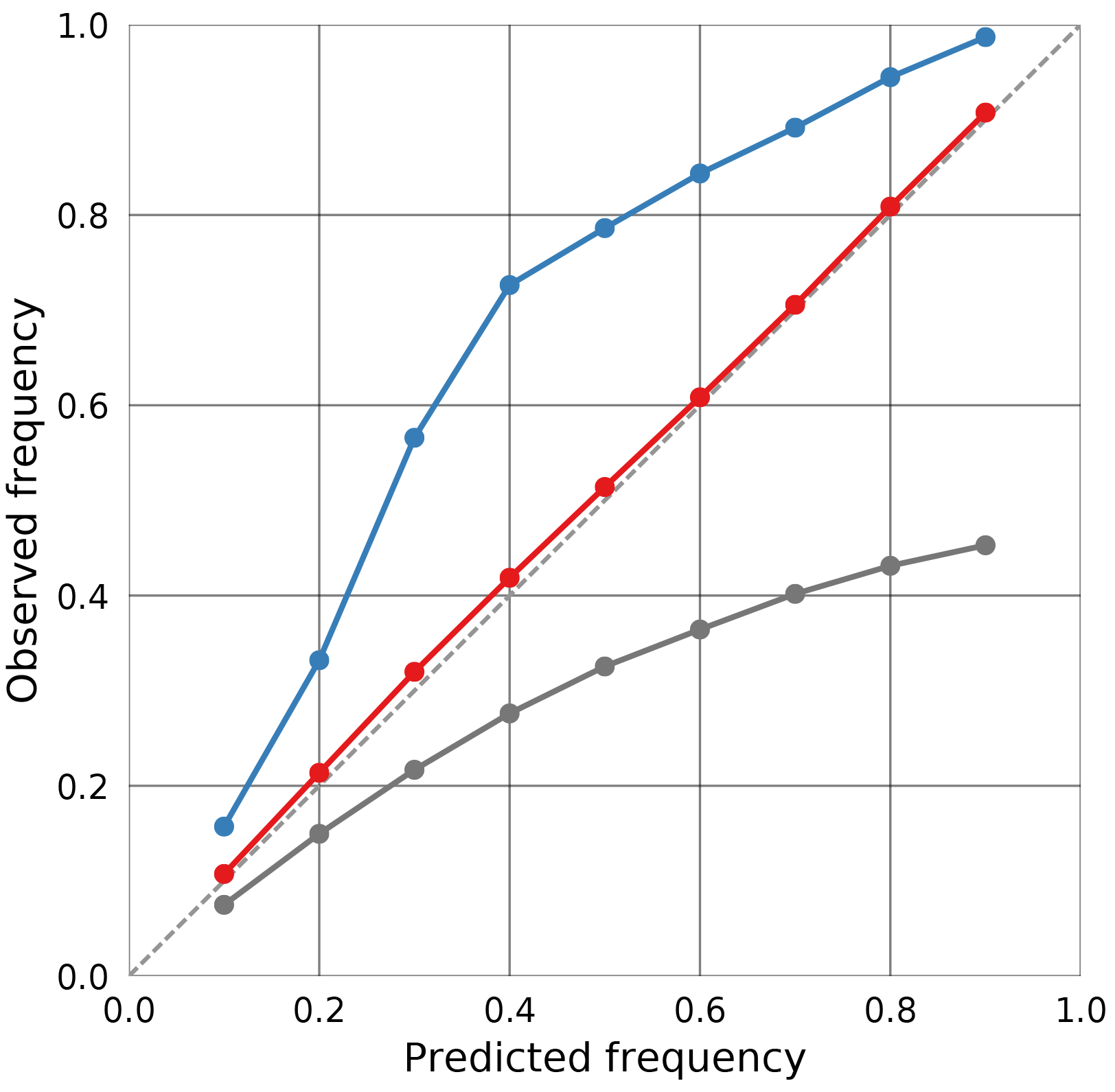
Figure 1 Example of a calibration plot displaying calibration curves for overly confident predictions (dark gray), well-calibrated predictions (red) and overly cautious predictions (blue).

3 Application to a synthetic retrieval case

In this section, a simulated retrieval of column water vapor (CWV) from passive microwave observations is used to benchmark the performance of BMCI and QRNN against MCMC simulation. The retrieval case has been set up to provide an idealized but realistic scenario in which the true a posteriori distribution can be approximated using MCMC simulation. The MCMC results can therefore be used as the reference to investigate the retrieval performance of QRNNs and BMCI. Furthermore the influence of different hyperparameters on the performance of the QRNN, as well as how the size of the training set and retrieval database impact the performance of QRNNs and BMCI, is investigated.

3.1 The retrieval

For this experiment, the retrieval of CWV from passive microwave observations over the ocean is considered. The state of the atmosphere is represented by profiles of temperature and water vapor concentrations on 15 pressure levels between 10³ and 10 hPa. The variability of these quantities has been estimated based on ECMWF ERA-Interim data (Dee et al., 2011) from the year 2016, restricted to latitudes between 23^∘ and 66^∘ N. Parametrizations of the multivariate distributions of temperature and water vapor were obtained by fitting a joint multivariate normal distribution to the temperature and the logarithm of water vapor concentrations. The fitted distribution represents the a priori knowledge on which the simulations are based.

3.1.1 Forward-model simulations

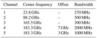
The Atmospheric Radiative Transfer Simulator (ARTS; Buehler et al., 2018) is used to simulate satellite observations of the atmospheric states sampled from the a priori distribution. The observations consist of simulated brightness temperatures from five channels around 23, 88, 165 and 183 GHz (cf. Table 1) of the ATMS sensor.

Table 1 Observation channels used for the synthetic retrieval of column water vapor.

The simulations take into account only absorption and emission from water vapor. Ocean surface emissivities are computed using the FASTEM-6 model (Kazumori and English, 2015) with an assumed surface wind speed of zero. The sea surface temperature is assumed to be equal to the temperature at the pressure level closest to the surface but no lower than 270 K. Sensor characteristics and absorption lines are taken from the ATMS sensor descriptions that are provided within the ARTS XML data package. Simulations are performed for a nadir-looking sensor and neglecting polarization. The observation uncertainty is assumed to be independent Gaussian noise with a standard deviation of 1 K.

3.1.2 MCMC implementation

The MCMC retrieval is based on a Python implementation of the Metropolis algorithm (Gelman et al., 2013) that has been developed within the context of this study. It is released as part of the typhon: tools for atmospheric research software package (The typhon authors, 2018).

The MCMC retrieval is performed in the space of atmospheric states described by the profiles of temperature and the logarithm of water vapor concentrations. The multivariate Gaussian distribution that has been obtained by fit to the ERA-Interim data is taken as the a priori distribution. A random walk is used as the proposal distribution, with its covariance matrix taken as the a priori covariance matrix. A single MCMC retrieval consists of eight independent runs, initialized with different random states sampled from the a priori distribution. Each run starts with a warm-up phase followed by an adaptive phase during which the covariance matrix of the proposal distribution is scaled adaptively to keep the acceptance rate of proposed states close to the optimal 21 % (Gelman et al., 2013). This is followed by a production phase during which 5000 samples of the a posteriori distribution are generated. Only 1 out of 20 generated samples is kept in order to decrease the correlation between the resulting states. Convergence of each simulation is checked by computing the scale reduction factor $\widehat{R}$ and the effective number of independent samples. The retrieval is accepted only if the scale reduction factor is smaller than 1.1 and the effective sample size larger than 100. Each MCMC retrieval generates a sequence of atmospheric states from which the column water vapor is obtained by integration of the water vapor concentration profile. The distribution of observed CWV values is then taken as the retrieved a posteriori distribution.

3.1.3 QRNN implementation

The implementation of quantile regression neural networks is based on the Keras Python package for deep learning (Chollet et al., 2015). It is also released as part of the typhon package.

For the training of quantile regression neural networks, the quantile loss function ℒ_τ(x_τ,x) has been implemented so that it can be used as a training loss function within the Keras framework. The function can be initialized with a sequence of quantile fractions ${\mathit{\tau }}_{\mathrm{1}},\mathrm{\dots },{\mathit{\tau }}_k$ allowing the neural network to learn to predict the corresponding quantiles $x_{{\mathit{\tau }}_{\mathrm{1}}},\mathrm{\dots },x_{{\mathit{\tau }}_k}$.

Custom data generators have been added to the implementation to incorporate information on measurement uncertainty into the training process. If the training data are noise free, the data generator can be used to add noise to each training batch according to the assumptions on measurement uncertainty. The noise is added immediately before the data are passed to the neural network, keeping the original training data noise free. This ensures that the network does not see the same noisy training sample twice during training, thus counteracting overfitting.

An adaptive form of stochastic batch gradient descent is used for the neural network training. During the training, loss is monitored on a validation set. When the loss on the validation set has not decreased for a certain number of epochs, the training rate is reduced by a given reduction factor. The training stops when a predefined minimum learning rate is reached.

The reconstruction of the CDF from the estimated quantiles is obtained by using the quantiles as nodes of a piecewise linear approximation and extending the first and last segments out to 0 and 1, respectively. This approximation is also used to compute the CRPS on the test data.

3.1.4 BMCI implementation

The BMCI method has likewise been implemented in Python and added to the typhon package. In addition to retrieving the first two moments of the posterior distribution, the implementation provides functionality to retrieve the posterior CDF using Eq. (4). Approximate posterior quantiles are computed by interpolating the inverse CDF at the desired quantile values. To compute the CRPS for a given retrieval, the trapezoidal rule is used to perform the integral over the values x_i in the retrieval database $\mathit{\{}{\mathit{y}}_i,x_i{\mathit{\}}}_{i=\mathrm{1}}^n$.

3.2 QRNN model selection

Just as with common neural networks, QRNNs have several hyperparameters that cannot be learned directly from the data but need to be tuned independently. For this study the dependence of the QRNN performance on its hyperparameters has been investigated. The results are included here as they may be a helpful reference for future applications of QRNNs.

For this analysis, hyperparameters describing the structure of the QRNN model are investigated separately from training parameters. The hyperparameters describing the structure of the QRNN are

1. the number of hidden layers,

2. the number of neurons per layer,

3. the type of activation function.

The training method described in Sect. 3.1.3 is defined by the following training parameters:

• 4.

  the batch size used for stochastic batch gradient descent,

• 5.

  the minimum learning rate at which the training is stopped,

• 6.

  the learning rate decay factor,

• 7.

  the number of training epochs without progress on the validation set before the learning rate is reduced.

3.2.1 Structural parameters

To investigate the influence of hyperparameters 1–3 on the performance of the QRNN, 10-fold cross validation on the training set consisting of 10⁶ samples has been used to estimate the performance of different hyperparameter configurations. As a performance metric, the mean quantile loss on the validation set averaged over all predicted quantiles for $\mathit{\tau }=\mathrm{0.05},\mathrm{0.1},\mathrm{0.2},\mathrm{\dots },\mathrm{0.9},\mathrm{0.95}$ is used. A grid search over a subspace of the configuration space was performed to find optimal parameters. The results of the analysis are displayed in Fig. 2. For the configurations considered, the layer width has the most significant effect on the performance. Nevertheless, only small performance gains are obtained by increasing the layer width to values above 64 neurons. Another general observation is that networks with three hidden layers generally outperform networks with fewer hidden layers. Networks using rectified linear unit (ReLU) activation functions not only achieve slightly better performance than networks using tanh or sigmoid activation functions but also show significantly lower variability. Based on these results, a neural network with three hidden layers, 128 neurons in each layer and ReLU activation functions has been selected for the comparison to BMCI.

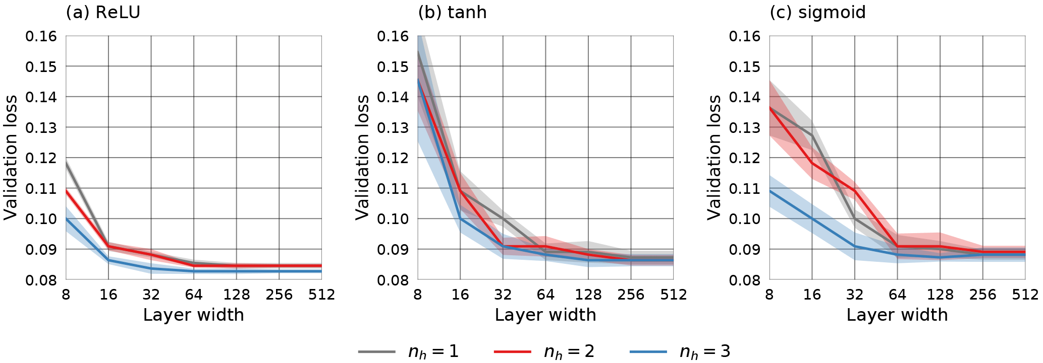
Figure 2 Mean validation set loss (solid lines) and standard deviation (shading) of different hyperparameter configurations with respect to layer width (number of neurons). Different lines display the results for different numbers of hidden layers n_h. The three panels show the results for ReLU, tanh and sigmoid activation functions.

3.2.2 Training parameters

For the optimization of training parameters 4–7, a very coarse grid search was performed, using only three different values for each parameter. In general, the training parameters showed only little effect (<2 % for the combinations considered here) on the QRNN performance compared to the structural parameters. The best cross-correlation performance was obtained for slow training with a small learning rate reduction factor of 1.5 and decreasing the learning rate only after 10 training epochs without reduction of the validation loss. No significant increase in performance could be observed for values of the learning rate minimum below 10⁻⁴. With respect to the batch size, the best results were obtained for a batch size of 128 samples.

3.3 Comparison against MCMC

In this section, the performance of a single QRNN and an ensemble of 10 QRNNs is analyzed. The predictions from the ensemble are obtained by averaging the predictions from each network in the ensemble. All tests in this subsection are performed for a single QRNN, the ensemble of QRNNs and BMCI. The retrieval database used for BMCI and the training of the QRNNs in this experiment consists of 10⁶ entries.

Figure 3 displays retrieval results for eight example cases. The choice of the cases is based on the Kolmogorov–Smirnov (KS) statistic, which corresponds to the maximum absolute deviation of the predicted CDF from the reference CDF obtained by MCMC simulation. A small KS value indicates a good prediction of the true CDF, while a high value is obtained for large deviations between predicted and reference CDF. The cases shown correspond to the 10th, 50th, 90th and 99th percentile of the distribution of KS values obtained using BMCI or a single QRNN. In this way they provide a qualitative overview of the performance of the methods.

In the displayed cases, both methods are generally successful in predicting the a posteriori distribution. Only for the 99th percentile of the KS value distribution does the BMCI prediction show significant deviations from the reference distribution. The jumps in the estimated a posteriori CDF indicate that the deviations are due to undersampling of the input space in the retrieval database. This results in excessively high weights attributed to the few entries close to the observation. For this specific case the QRNN provides a better estimate of the a posteriori CDF even though both predictions are based on the same data.

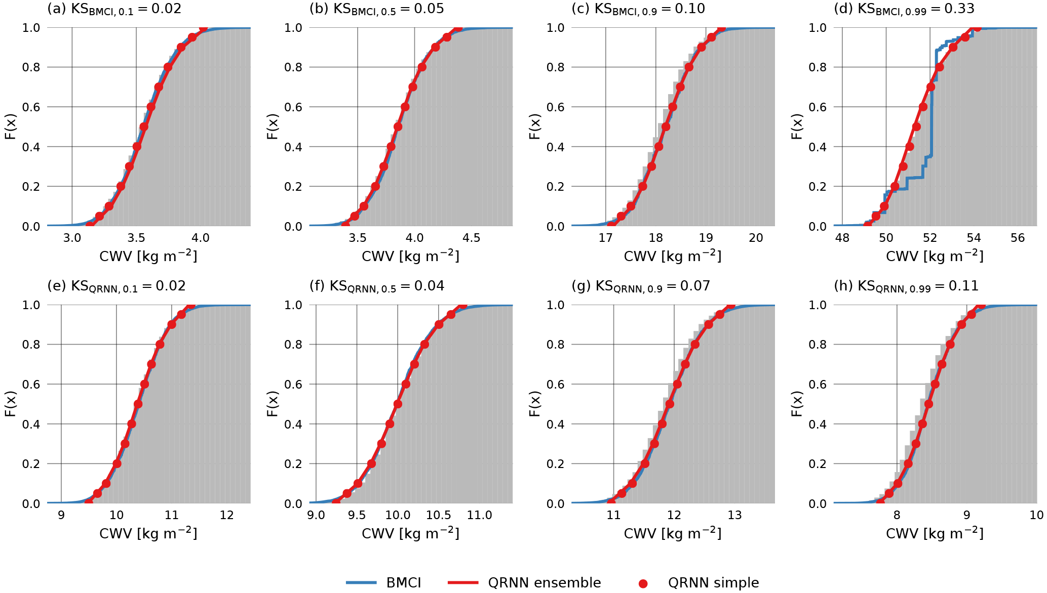
Figure 3 Retrieved a posteriori CDFs obtained using MCMC (gray), BMCI (blue), a single QRNN (red line) and an ensemble of QRNNs (red marker). Cases displayed in the first row correspond to the 1st, 50th, 90th and 99th percentiles of the distribution of the Kolmogorov–Smirnov statistic of BMCI compared to the MCMC reference. The second row displays the same percentiles of the distribution of the Kolmogorov–Smirnov statistic of the single-QRNN predictions compared to MCMC.

Another way of displaying the estimated a posteriori distribution is by means of its probability density function (PDF), which is defined as the derivative of its CDF. For the QRNN, the PDF is approximated by simply deriving the piecewise linear approximation to the CDF and setting the boundary values to zero. For BMCI, the a posteriori PDF can be approximated using a histogram of the CWV values in the database weighted by the corresponding weights w_i(y). The PDFs for the cases corresponding to the CDFs show in Fig. 3 are shown in Fig. 4.

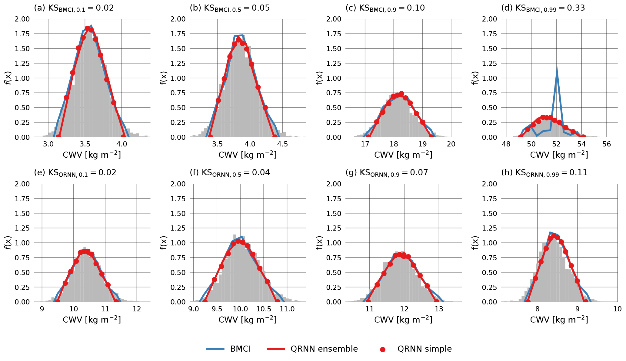
Figure 4 Retrieved a posteriori PDFs corresponding to the CDFs displayed in Fig. 3 obtained using MCMC (gray), BMCI (blue), a single QRNN (red line) and an ensemble of QRNNs (red marker).

To obtain a more comprehensive view on the performance of QRNNs and BMCI, the predictions obtained from both methods are compared to those obtained from MCMC for 6500 test cases. For the comparison, let the effective quantile fraction τ_eff be defined as the fraction of MCMC samples that are less than or equal to the predicted quantile $\widehat{x_{\mathit{\tau }}}$ obtained from QRNN or BMCI. In general, the predicted quantile $\widehat{x_{\mathit{\tau }}}$ will not correspond exactly to the true quantile x_τ but rather to an effective quantile $x_{{\mathit{\tau }}_{\text{eff}}}$, defined by the fraction τ_eff of the samples of the distribution that are smaller than or equal to the predicted value $\widehat{x_{\mathit{\tau }}}$. The resulting distributions of the effective quantile fractions for BMCI and QRNNs are displayed in Fig. 5 for the estimated quantiles for $\mathit{\tau }=\mathrm{0.1},\mathrm{0.2},\mathrm{\dots },\mathrm{0.9}$.

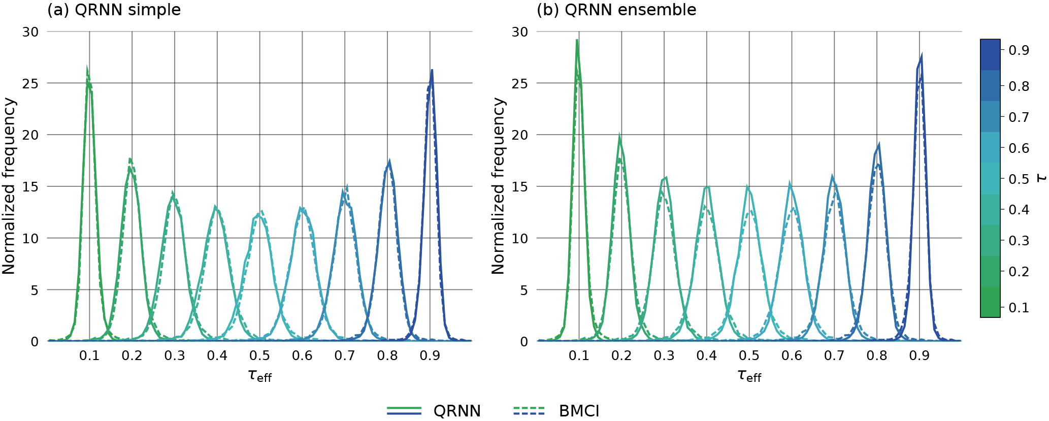
Figure 5 Distribution of effective quantile fractions τ_eff achieved by QRNN and BMCI on the test data. Panel (a) displays the performance of a single QRNN compared to BMCI; panel (b) displays the performance of the ensemble.

For an ideal estimator of the quantile x_τ, the resulting distribution would be a delta function centered at τ. Due to the estimation error, however, the τ_eff values are distributed around the true quantile fraction τ. The results show that both BMCI and QRNN provide fairly accurate estimates of the quantiles of the a posterior distribution. Furthermore, all methods yield equally good predictions, making the distributions virtually identical.

3.4 Training set size impact

Finally, we investigate how the size of the training data set used in the training of the QRNN (or as a retrieval database for BMCI) affects the performance of the retrieval method. This has been done by randomly generating training subsets from the original training data with sizes logarithmically spaced between 10³ and 10⁶ samples. For each size, five random training subsets have been generated and used to retrieve the test data with a single QRNN and BMCI. As test data, a separate test set consisting of 10⁵ simulated observation vectors and corresponding CWV values is used.

Figure 6 displays the means of the mean absolute percentage error (MAPE, panel a) and the mean CRPS (panel b) achieved by both methods on the differently sized training sets. For the computation of the MAPE, the CWV prediction is taken as the median of the estimated a posteriori distribution obtained using QRNNs or BMCI. This value is compared to the true CWV value corresponding to the atmospheric state that has been used in the simulation. As expected, the performance of both methods improves with the size of the training set. With respect to the MAPE, both methods perform equally well for a training set size of 10⁶, but the QRNN outperforms BMCI for all smaller training set sizes. With respect to CRPS, a similar behavior is observed. These are reassuring results, as they indicate that not only the accuracy of the predictions (measured by the MAPE and CRPS) improves as the amount of training data increases, but also their calibration (measured only by the CRPS).

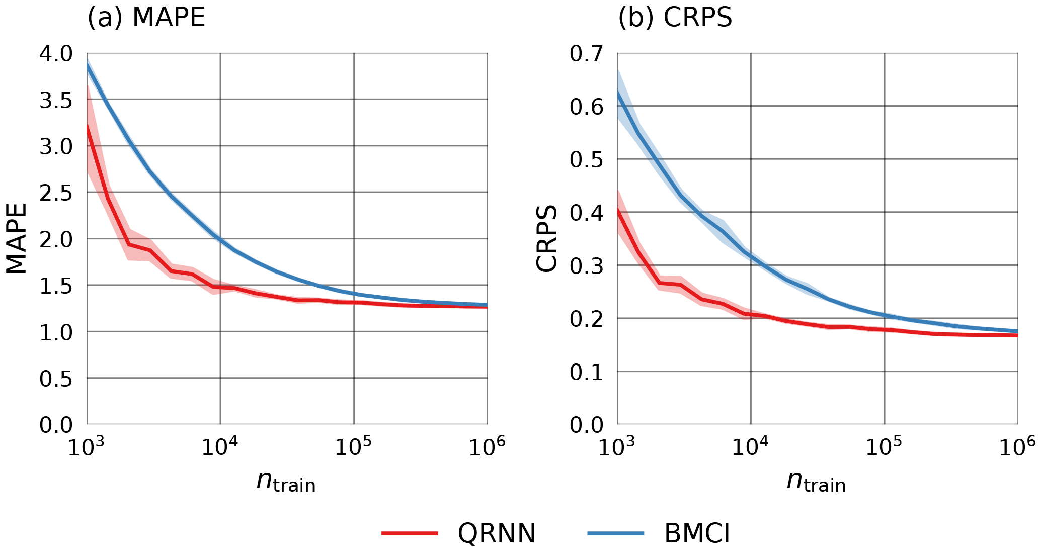
Figure 6 MAPE (a) and CRPS (b) achieved by QRNN (red) and BMCI (blue) on the test set using differently sized training sets and retrieval databases. For each size, five random subsets of the original training data were generated. The lines display the means of the observed values. The shading indicates the range of ±σ around the mean.

Finally, the mean of the quantile loss ℒ_τ on the test set for τ=0.1, 0.5 and 0.9 has been considered (Fig. 7). Qualitatively, the results are similar to the ones obtained using MAPE and CRPS. The QRNN outperforms BMCI for smaller training set sizes but converges to similar values for training set sizes of 10⁶.

Figure 7 Mean quantile loss for different training set sizes n_train and τ=0.1, 0.5 and 0.9.

The results presented in this section indicate that QRNNs can, at least under idealized conditions, be used to estimate the a posteriori distribution of Bayesian retrieval problems. Moreover, they were shown to work equally well as BMCI for large data sets. What is interesting is that, for smaller data sets, QRNNs even provide better estimates of the a posteriori distribution than BMCI. This indicates that QRNNs provide a better representation of the functional dependency of the a posteriori distribution on the observation data, thus achieving better interpolation in the case of scarce training data. Nonetheless, it remains to be investigated if this advantage can also be observed for real-world data.

A possible approach to handling scarce retrieval databases with BMCI is to artificially increase the assumed measurement uncertainty. This has not been performed for the BMCI results presented here and may improve the performance of the method. The difficulty with this approach is that the method formulation is based on the assumption of a sufficiently large database and thus can, at least formally, not handle scarce training data. Finding a suitable way to increase the measurement uncertainty would thus require either additional methodological development or invention of a heuristic approach, both of which are outside the scope of this study.

4 Retrieving cloud top pressure from MODIS using QRNNs

In this section, QRNNs are applied to retrieve cloud top pressure (CTP) using observations from the Moderate Resolution Imaging Spectroradiometer (MODIS; Platnick et al., 2003). The experiment is based on the work by Håkansson et al. (2018), who developed the NN-CTTH algorithm, a neural-network-based retrieval of cloud top pressure. A QRNN-based CTP retrieval is compared to the NN-CTTH algorithm, and how QRNNs can be used to estimate the retrieval uncertainty is investigated.

4.1 Data

The QRNN uses the same data for training as the reference NN-CTTH algorithm. The data set consists of MODIS Level 1B data (MODIS Characterization Support Team, 2015a, b) collocated with cloud properties obtained from CALIOP (Cloud-Aerosol Lidar with Orthogonal Polarization; Winker et al., 2009). The top layer pressure variable from the CALIOP data is used as a retrieval target. The data were taken from all orbits from 24 days (the 1st and 14th of every month) from the year 2010. In Håkansson et al. (2018) multiple neural networks are trained using varying combinations of input features derived from different MODIS channels and ancillary NWP data in order to compare retrieval performance for different inputs. Of the different neural network configurations presented in Håkansson et al. (2018), the version denoted by NN-AVHRR (development version of the NN-CTTH algorithm which uses only channels available from the Advanced Very High Resolution Radiometer (AVHRR)) is used for comparison against the QRNN. This version uses only the 11 and 12 µm channels from MODIS. In addition to single pixel input, the input features comprise structural information in the form of various statistics computed on a 5×5 neighborhood around the center pixel. The ancillary numerical weather prediction (NWP) data provided to the network consist of surface pressure and temperature, temperatures at five pressure levels and column-integrated water vapor. These are also the input features that are used for the training of the QRNN. The training data used for the QRNN are the training and during-training validation set from Håkansson et al. (2018). The comparison to the NN-AVHRR version of the NN-CTTH algorithm uses the data set for testing under development from Håkansson et al. (2018).

4.2 Training

The same training scheme as described in Sect. 3.1.3 is used for the training of the QRNNs. The training progress, based on which the learning rate is reduced or training aborted, is monitored using the during-training validation data set from Håkansson et al. (2018). After performing a grid search (results not shown) over width, depth and minibatch size, the best performance on the validation set was obtained for networks with four layers with 64 neurons each, ReLU activation functions and a batch size of 128 samples.

The main difference in the training process compared to the experiment from the previous section is how measurement uncertainties are incorporated. For the simulated retrieval, the training data was noise free, so measurement uncertainties could be realistically represented by adding noise according to the sensor characteristics. This is not the case for MODIS observations; instead, adversarial training is used here to ensure well-calibrated predictions. For the tuning of the perturbation parameter δ_adv (cf. Sect. 2.3.4), the calibration on the during-training validation set was monitored using a calibration plot. Ideally, it would be desirable to use a separate data set to tune this parameter, but this was sufficient in this case to achieve good results on the test data. The calibration curves obtained using different values of δ_adv are displayed in Fig. 8. It can be seen from the plot that without adversarial training (δ_adv=0) the predictions obtained from the QRNN are overly confident, leading to prediction intervals that underrepresent the uncertainty in the retrieval. Since adversarial training may be viewed as a way of representing observation uncertainty in the training data, larger values of δ_adv lead to less confident predictions. Based on these results, δ_adv=0.05 is chosen for the training.

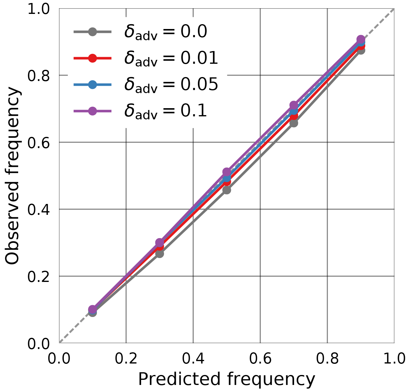
Figure 8 Calibration of the QRNN prediction intervals on the validation set used during training. The curves display the results for no adversarial training (δ_adv=0) and adversarial training with perturbation factor ${\mathit{\delta }}_{\text{adv}}=\mathrm{0.01},\mathrm{0.05},\mathrm{0.1}$.

Except for the use of adversarial training, the structure of the underlying network and the training process of the QRNN are fairly similar to what is used for the NN-CTTH retrieval. The QRNN uses four instead of two hidden layers with 64 neurons in each of them instead of 30 in the first and 15 in second layer. While this makes the neural network used in the QRNN slightly more complex, this should not be a major drawback since computational performance is generally not critical for neural network retrievals.

4.3 Prediction accuracy

Most data analysis will likely require a single predicted value for the cloud top pressure. To derive a point value from the QRNN prediction, the median of the estimated a posteriori distribution is used.

The distributions of the resulting median pressure values on the testing-during-development data set are displayed in Fig. 9 together with the retrieved pressure values from the NN-CTTH algorithm. The distributions are displayed separately for low, medium and high clouds (as classified by the CALIOP feature classification flag) as well as the complete data set. From these results it can be seen that the values predicted by the QRNN have stronger peaks low in the atmosphere for low clouds and high in the atmosphere for high clouds. For medium clouds the peak is more spread out and has heavier tails low and high in the atmosphere than the values retrieved by the NN-CTTH algorithm.

Figure 10 displays the error distributions of the predicted CTP values on the testing-during-development data set, again separated by cloud type as well as for the complete data set. Both the simple QRNN and the ensemble of QRNNs perform slightly better than the NN-CTTH algorithm for low and high clouds. For medium clouds, no significant difference in the performance of the methods can be observed. The ensemble of QRNNs seems to slightly improve upon the prediction accuracy of a single QRNN, but the difference is likely negligible. Compared to the QRNN results, the CTP predicted by NN-CTTH is biased low for low clouds and biased high for high clouds.

Even though both the QRNN and the NN-CTTH retrieval use the same input and training data, the predictions from both retrievals differ considerably. Using the Bayesian framework, this can likely be explained by the fact that the two retrievals estimate different statistics of the a posteriori distribution. The NN-CTTH algorithm has been trained using a squared error loss function which will lead the algorithm to predict the mean of the a posteriori distribution. The QRNN retrieval, on the other hand, predicts the median of the a posteriori distribution. Since the median minimizes the expected absolute error, it is expected that the CTP values predicted by the QRNN yield overall smaller errors.

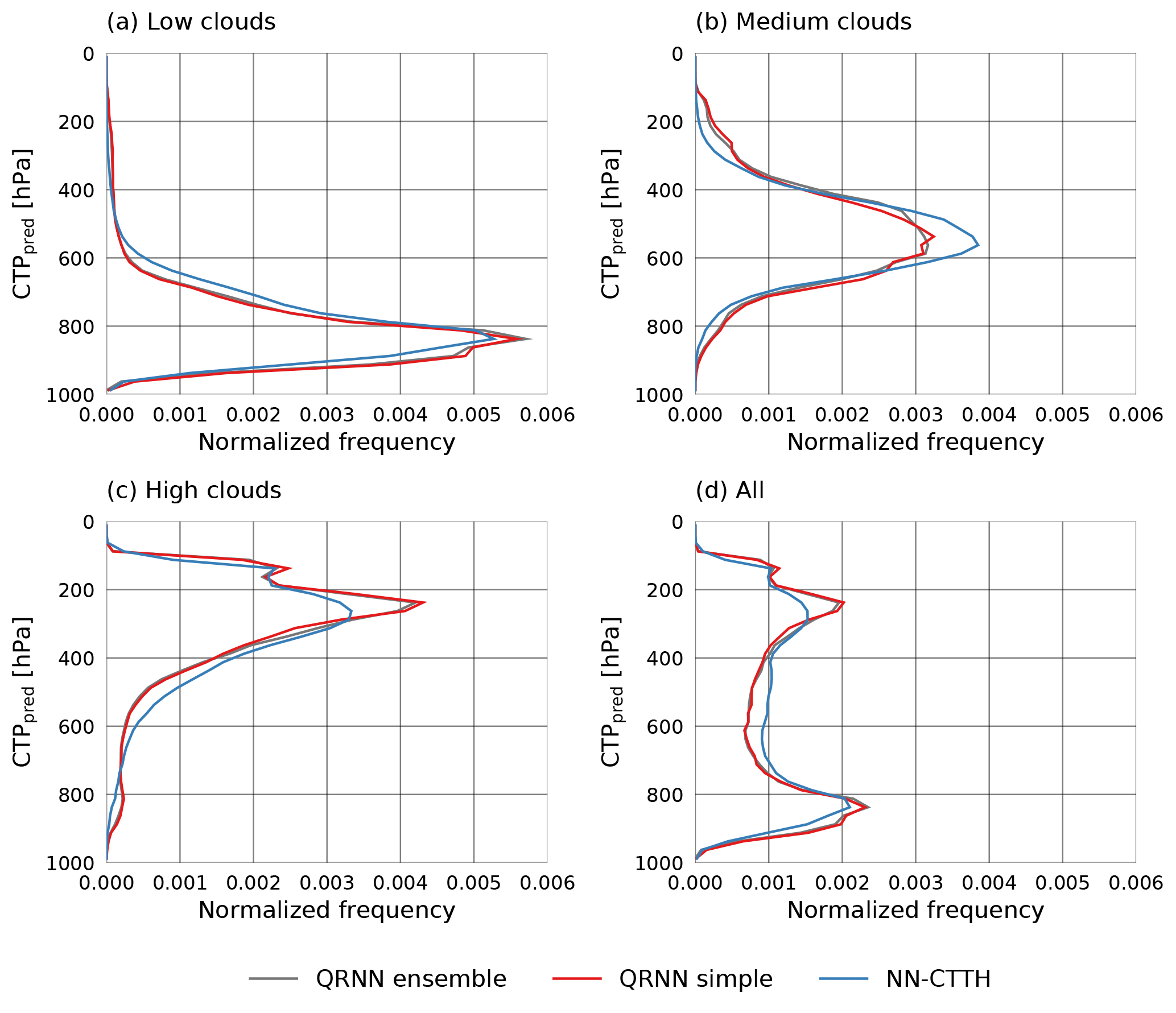
Figure 9 Distributions of predicted CTP values (CTP_pred) for high clouds (a), medium clouds (b), low clouds (c) and the complete test set (d).

Figure 10 Error distributions of predicted CTP values (CTP_pred) with respect to CTP from CALIOP (CTP_ref) for high clouds (a), medium clouds (b), low clouds (c) and the complete test set (d).

4.4 Uncertainty estimation

The NN-CTTH algorithm retrieves CTP but does not provide case-specific uncertainty estimates. Instead, an estimate of uncertainty is provided in the form of the observed mean absolute error (MAE) on the test set. In order to compare these uncertainty estimates with those obtained using QRNNs, Gaussian error distributions are fitted to the observed error based on the observed MAE and mean squared error (MSE). A Gaussian error model is chosen here as it is arguably the most common distribution used to represent random errors.

A plot of the errors observed on the testing-during-development data set and the fitted Gaussian error distributions is displayed in panel a of Fig. 11. The fitted error curves correspond to the Gaussian probability density functions with the same MAE and MSE as observed on the test data. Panel b displays the observed error together with the predicted error obtained from a single QRNN. The predicted error is computed as the deviation of a random sample of the estimated a posteriori distribution from its median. The fitted Gaussian error distributions clearly do not provide a good fit to the observed error. On the other hand, the predicted errors obtained from the QRNN a posteriori distributions yield good agreement with the observed error. This indicates that the QRNN successfully learned to predict retrieval uncertainties. Furthermore, the results show that the ensemble of QRNNs actually provides a slightly worse fit to the observed error than a single QRNN. An ensemble of QRNNs thus does not necessarily improve the calibration of the predictions.

The Gaussian error model based on the MAE fit has also been used to produce prediction intervals for the CTP values obtained from the NN-CTTH algorithm. Figure 12 displays the resulting calibration curves for the NN-CTTH algorithm, a simple QRNN and an ensemble of QRNNs. The results support the finding that a single QRNN is able to provide well-calibrated probabilistic predictions of the a posteriori distribution. The calibration curve for the ensemble predictions is virtually identical to that for the single network. The NN-CTTH predictions using a Gaussian fit are not as well calibrated and tend to provide prediction intervals that are too wide for p=0.1, 0.3, 0.5 and 0.7 but overly narrow intervals for p=0.9.

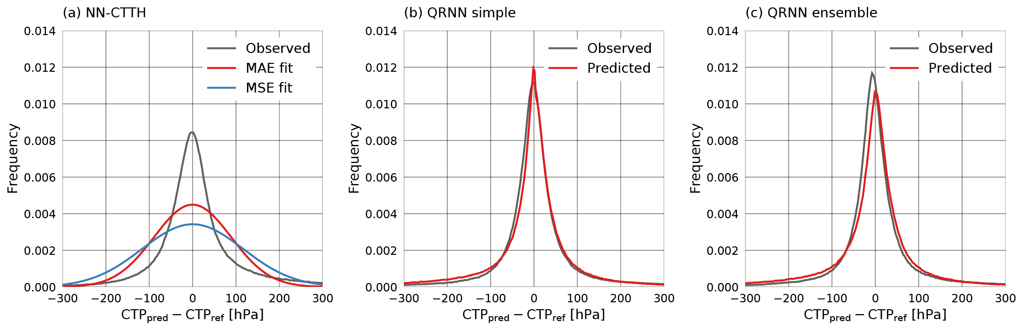
Figure 11 Predicted and observed error distributions. Panel (a) displays the observed error for the NN-CTTH retrieval as well as the Gaussian error distributions that have been fitted to the observed error distribution based on the MAE and MSE. Panel (b) displays the observed test set error for a single QRNN as well as the predicted error obtained as the deviation of a random sample of the predicted a posteriori distribution from the median. Panel (c) displays the same for the ensemble of QRNNs.

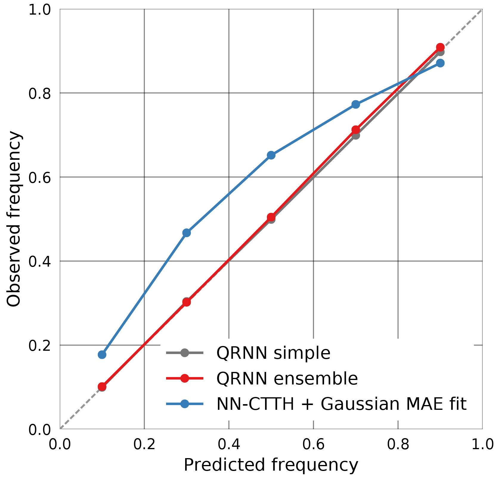
Figure 12 Calibration plot for prediction intervals derived from the Gaussian error model for the NN-CTTH algorithm (blue), the single QRNN (dark gray) and the ensemble of QRNNs (red).

4.5 Sensitivity to a priori distribution

As shown above, the predictions obtained from the QRNN are statistically consistent in the sense that they predict probabilities that match observed frequencies when applied to test data. This, however, requires that the test data are statistically consistent with the training data. Statistically consistent here means that both data sets come from the same generating distribution or, in more Bayesian terms, the same a priori distribution. What happens when this is not the case can be seen when the calibration with respect to different cloud types is computed. Figure 13 displays calibration curves computed separately for low, medium and high clouds. As can be seen from the plot, the QRNN predictions are no longer equally well calibrated. Viewed from the Bayesian perspective, this is not very surprising as CTP values for median clouds have a significantly different a priori distribution compared to CTP values for all cloud types, thus giving different a posteriori distributions.

For the NN-CTTH algorithm, the results look different. While for low clouds the calibration deteriorates, the calibration is even slightly improved for high clouds. This is not surprising as the Gaussian fit may be more appropriate on different subsets of the test data.

5 Conclusions

In this article, quantile regression neural networks have been proposed as a method to estimate a posteriori distributions of Bayesian remote sensing retrievals. They have been applied to two retrievals of scalar atmospheric variables. It has been demonstrated that QRNNs are capable of providing accurate and well-calibrated probabilistic predictions in agreement with the Bayesian formulation of the retrieval problem.

The synthetic retrieval case presented in Sect. 3 shows that the conditional distribution learned by the QRNN is the same as the Bayesian a posteriori distribution obtained from methods that are directly based on the Bayesian formulation. This in itself seems worthwhile to note, as it reveals the importance of the training set statistics that implicitly represent the a priori knowledge. On the synthetic data set, QRNNs compare well to BMCI and even perform better for small data sets. This indicates that they are able to handle the “curse of dimensionality” (Friedman et al., 2001) better than BMCI, which would make them more suitable for the application to retrieval problems with high-dimensional measurement spaces.

While the optimization of computational performance of the BMCI method has not been investigated in this work, at least compared to a naive implementation of BMCI, QRNNs allow for retrievals that are at least 1 order of magnitude faster. QRNN retrievals can be easily parallelized, and hardware optimized implementations are available for all modern computing architectures, thus providing very good performance out of the box.

Based on these very promising results, the next step in this line of research should be to compare QRNNs and BMCI on a real retrieval case to investigate if the findings from the simulations carry over to the real world. If this is the case, significant reductions in the computational cost of operational retrievals and maybe even better retrieval performance could be achieved using QRNNs.

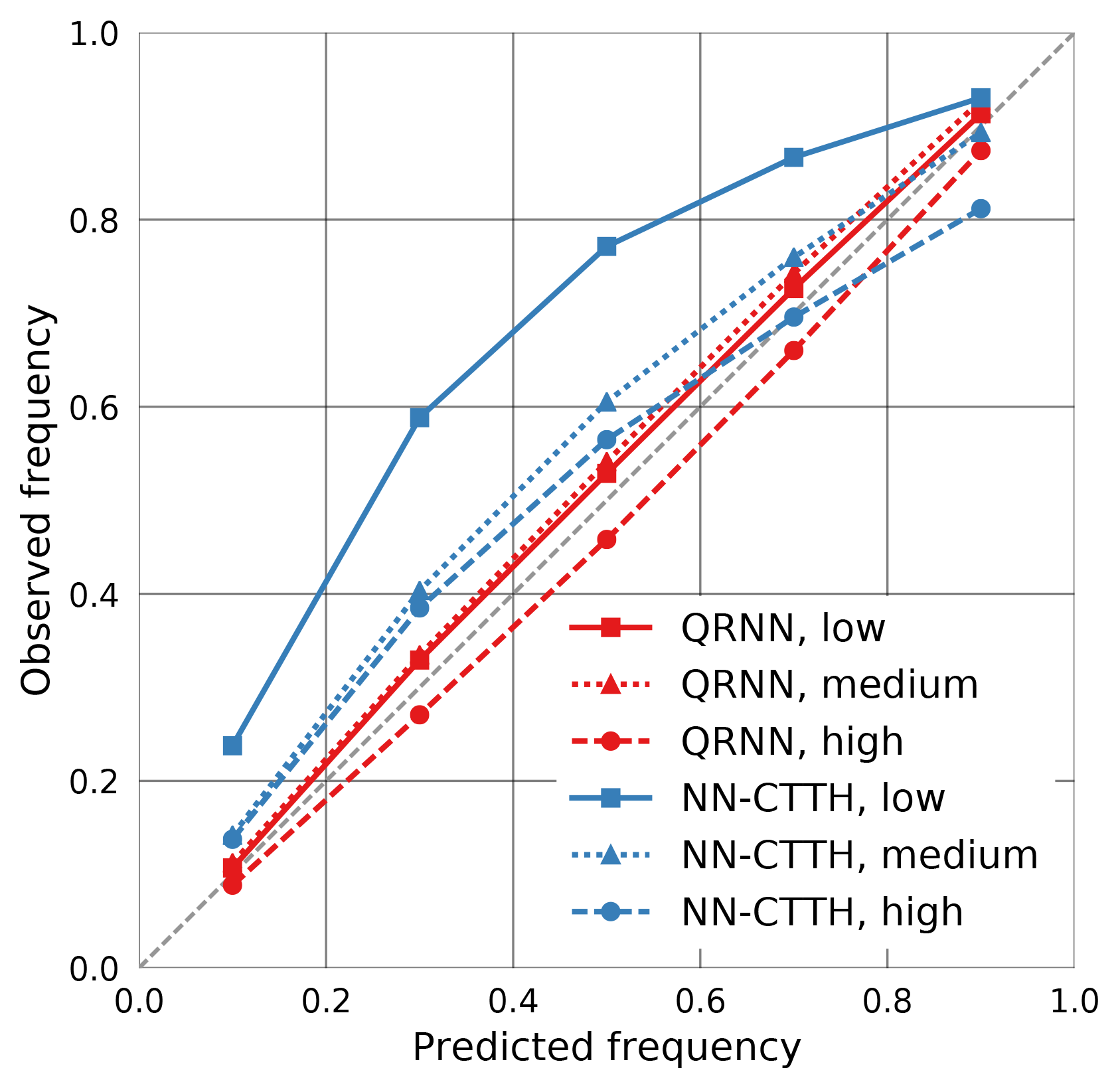
Figure 13 Calibration of the prediction intervals obtained from NN-CTTH (blue) and a single QRNN (red) with respect to specific cloud types.

In the second retrieval application presented in this article, QRNNs have been used to retrieve cloud top pressure from MODIS observations. The results show that not only are QRNNs able to improve upon state-of-the-art retrieval accuracy, but they can also learn to predict retrieval uncertainty. The ability of QRNNs to provide statistically consistent, case-specific uncertainty estimates should make them a very interesting alternative to non-probabilistic neural network retrievals. Nonetheless, the sensitivity of the QRNN approach to a priori assumptions has also been demonstrated. The posterior distribution learned by the QRNN depends on the validity of the a priori assumptions encoded in the training data. In particular, accurate uncertainty estimates can only be expected if the retrieved observations follow the same distribution as the training data. This, however, is a limitation inherent to all empirical methods.

The second application case presented here demonstrated the ability of QRNNs to represent non-Gaussian retrieval errors. While, as shown in this study, this is also the case for BMCI (Eq. 4), it is common in practice to estimate only mean and standard deviation of the a posteriori distribution. Furthermore, implementations usually assume Gaussian measurement errors, which is an unlikely assumption if the observations in the retrieval database contain modeling errors. By requiring no assumptions whatsoever on the involved uncertainties, QRNNs may provide a more suitable way of representing (non-Gaussian) retrieval uncertainties.

The application of the Bayesian framework to neural network retrievals opens the door to a number of interesting applications that could be pursued in future research. It would for example be interesting to investigate if the a priori information can be separated from the information contained in the retrieved measurement. This would make it possible to remove the dependency of the probabilistic predictions on the a priori assumptions, which can currently be considered a limitation of the approach. Furthermore, estimated a posteriori distributions obtained from QRNNs could be used to estimate the information content in a retrieval following the methods outlined by Rodgers (2000).

In this study only the retrieval of scalar quantities was considered. Another aspect of the application of QRNNs to remote sensing retrievals that remains to be investigated is how they can be used to retrieve vector-valued retrieval quantities, such as concentration profiles of atmospheric gases or particles. While the generalization to marginal, multivariate quantiles should be straightforward, it is unclear whether a better approximation of the quantile contours of the joint a posteriori distribution can be obtained using QRNNs.