the Creative Commons Attribution 4.0 License.
the Creative Commons Attribution 4.0 License.
 | 25 Feb 2019
Remote sensing of cloud droplet radius profiles using solar reflectance from cloud sides – Part 1: Retrieval development and characterization
Tobias Zinner
Tobias Kölling
Bernhard Mayer
Convective clouds play an essential role for Earth's climate as well as for regional weather events since they have a large influence on the radiation budget and the water cycle. In particular, cloud albedo and the formation of precipitation are influenced by aerosol particles within clouds. In order to improve the understanding of processes from aerosol activation, from cloud droplet growth to changes in cloud radiative properties, remote sensing techniques become more and more important. While passive retrievals for spaceborne observations have become sophisticated and commonplace for inferring cloud optical thickness and droplet size from cloud tops, profiles of droplet size have remained largely uncharted territory for passive remote sensing. In principle they could be derived from observations of cloud sides, but faced with the small-scale heterogeneity of cloud sides, “classical” passive remote sensing techniques are rendered inappropriate. In this work the feasibility is demonstrated to gain new insights into the vertical evolution of cloud droplet effective radius by using reflected solar radiation from cloud sides. Central aspect of this work on its path to a working cloud side retrieval is the analysis of the impact unknown cloud surface geometry has on effective radius retrievals. This study examines the sensitivity of reflected solar radiation to cloud droplet size, using extensive 3-D radiative transfer calculations on the basis of realistic droplet size resolving cloud simulations. Furthermore, it explores a further technique to resolve ambiguities caused by illumination and cloud geometry by considering the surroundings of each pixel. Based on these findings, a statistical approach is used to provide an effective radius retrieval. This statistical effective radius retrieval is focused on the liquid part of convective water clouds, e.g., cumulus mediocris, cumulus congestus, and trade-wind cumulus, which exhibit well-developed cloud sides. Finally, the developed retrieval is tested using known and unknown cloud side scenes to analyze its performance.
- Article
(11218 KB) - Full-text XML
- BibTeX
- EndNote


Various methods exist for inferring optical properties (e.g., optical thickness and cloud droplet effective radius) from observation of cloud tops, using information about the scattered and absorbed radiation in the solar spectrum (e.g., Plass and Kattawar, 1968; King, 1987). Phase detection is the first step for every cloud property retrieval. Spectral absorption differences in the near-infrared or brightness temperature differences in the thermal infrared are commonly used to distinguish between liquid water and ice (e.g., Nakajima and King, 1990). Various operational techniques exist to retrieve microphysical cloud properties like cloud thermodynamic phase and effective particle size (e.g., Han et al., 1994; Platnick et al., 2001; Roebeling et al., 2006).
Remote sensing of cloud and aerosol parameters is mostly done by use of multi-spectral sensors, i.e., using only a limited number of spectral bands. Common examples of spaceborne imagers are the Advanced Very High Resolution Radiometer (AVHRR), the Moderate Resolution Imaging Spectroradiometer (MODIS), and the Spinning Enhanced Visible Infrared Imager (SEVIRI). However, there are concerns about measurement artifacts influencing retrievals of aerosol and cloud properties caused by small-scale cloud inhomogeneity which are unresolved by the coarse spatial resolution of spaceborne platforms (Zinner and Mayer, 2006; Marshak et al., 2006b; Varnai and Marshak, 2007).
Non-imaging systems like the Solar Spectral Flux Radiometer (SSFR, Pilewskie et al., 2003) or the Spectral Modular Airborne Radiation measurement sysTem (SMART, Wendisch et al., 2001; Wendisch and Mayer, 2003) were used for cloud remote sensing from the ground (McBride et al., 2011; Jäkel et al., 2013) or aircraft (Ehrlich et al., 2008; Eichler et al., 2009; Schmidt et al., 2007).
Scientific objectives and scope of this work
In order to observe the vertical development of convective cloud microphysics, Marshak et al. (2006a) and Martins et al. (2011) proposed cloud side scanning measurements while Zinner et al. (2008) and Ewald et al. (2013) presented concrete steps towards a cloud side retrieval for profiles of phase and particle size. Similar to previous satellite retrievals they propose using solar radiation in the near-visible to near-infrared spectral regions reflected by cloud sides. The vertical dimension of these observations especially should reflect aspects of cloud–aerosol interaction, as well as the mixing of cloudy and ambient air (Martins et al., 2011; Rosenfeld et al., 2012). However, the retrieval of cloud microphysical profiles demands a high spatial resolution on the order of 100 m or better. In turn, the high spatial resolution necessitates a method to consider 3-D radiative transfer effects.
Albeit sophisticated, the studies of Zinner et al. (2008) and Ewald et al. (2013) are limited to an idealized geometry and simplified cloud microphysics. First, they focus on a space-like perspective for a fixed viewing zenith and scattering angle above the cloud field, where sun and sensor have the same azimuth. Therefore, their studies lack the varying geometries of an airborne perspective and avoid the challenge of identifying suitable observation positions within the cloud field. Moreover, the spatial resolution of their model cloud fields of 250 m is still rather coarse for an airborne perspective of cloud sides. Following from this, the effective radius is only parameterized in their studies. For all cloud fields, the effective radius profile is calculated by using a sub-adiabatic ascent of one air parcel in the context of a fixed cloud condensation nuclei (CCN) concentration. Finally, the approach was not tested for an inherent bias for detecting larger effective radii with increasing cloud height, a potential pitfall that could be caused by the prior information contained in the forward calculations.
Since the diverse perspectives and the high spatial resolution of airborne cloud side measurements hampered the application of the approach presented by Zinner et al. (2008) and Ewald et al. (2013) until now, the present work will extend and test their ideas in the context of an airborne perspective. In the course of this Part 1, the following scientific objectives will be addressed:
-
extending the existing approach to realistic airborne perspectives and development of methods to test the sensitivity of reflected radiances from cloud sides to cloud droplet radius, where the observer position is located within the cloud field;
-
investigating and mitigating of 3-D radiative effects which can interfere with the proposed cloud side remote sensing technique;
-
testing of the approach in the context of realistic and explicit cloud microphysics with a specific focus on potential biases caused by the prior contained in the forward calculations.
The target of this work is the liquid part of convective water clouds, e.g., cumulus mediocris, cumulus congestus, and trade-wind cumulus, which exhibit well-developed cloud sides. During September 2014, images of such cloud sides were acquired with the spectrometer of the Munich Aerosol Cloud Scanner (specMACS, Ewald et al., 2016) over the Amazon rainforest near Manaus, Brazil. The measurements were performed during the ACRIDICON-CHUVA campaign (Wendisch et al., 2016), during which the specMACS instrument was deployed on the German research aircraft HALO (Krautstrunk and Giez, 2012), mounted in a side-looking configuration. The campaign focused on aerosol–cloud–precipitation interactions over the Amazon rainforest. More specifically, the campaign investigated the impact of wildfire aerosols on cumulus clouds and on their later development into deep convection. During the campaign flights, the aerosol background and the small-scale convection in their early stages was probed in low-level flight legs between 1 and 3 km altitude. At cloud base level, mean CCN concentrations ranged between 250 and 2000 cm−3 (Andreae et al., 2018). The specMACS measurements were done of cumulus clouds in a distance of 2 to 6 km and with top heights between 1.5 and 3 km. Subsequently, vertical profile flights were performed to measure the microphysical properties of the developing convection in situ. This paper (Part 1) develops a statistical effective radius retrieval for these non-glaciated cumulus clouds which were measured during the low-level flights. Part 2 of this work presents the application to airborne specMACS data collected during the ACRIDICON-CHUVA and comparison to in situ measurements.
This study is organized as follows: Sect. 2 shortly recapitulates established methods and introduces the new cloud model data set with explicit cloud microphysics. New methods for selecting suitable cloud sides and connect 3-D radiances with 3-D cloud microphysics will be described in Sect. 3. In Sect. 4, the sensitivity of reflected radiances to cloud droplet radii is examined for a simple, spherical cloud geometry, before moving the focus to the more realistic cloud side scenes. With the obtained insights, a method is developed to mitigate 3-D radiative effects by using additional information from surrounding pixels. The extensive three-dimensional (3-D) radiative transfer simulations of cloud sides, which form the basis of the statistical effective radius retrieval, are described in Sect. 5. In contrast to previous studies, different aerosol backgrounds are now also considered. For the retrieval, the results for different CCN concentrations are combined within one lookup table to be independent of a priori knowledge of NCCN. Finally, the developed retrieval is tested in Sect. 6, with unknown scenes of cloud sides and different aerosol backgrounds. Furthermore, the retrieval is analyzed for potential biases.
2.1 Statistical approach
The derivation of vertical profiles of cloud microphysics from radiance reflected by cloud sides is a strongly under-determined problem. The statistical approach tries to provide a probability of a specific cloud microphysical state (e.g., effective radius) where a deterministic inversion is impossible due to ambiguities caused by an unknown cloud geometry. This work will follow the approach proposed by Marshak et al. (2006a) and Zinner et al. (2008), who developed a statistical method to account for three-dimensional radiative effects on complex-shaped cloud sides. In their studies, a large number of 3-D radiance simulations of cloud data sets provide a database for a statistical effective radius retrieval.
More specifically, a forward model is used to perform an ensemble of radiative transfer calculations to estimate the joint probability to observe the joint occurrence of radiances L0.87, L2.10 and effective radius reff. The likelihood of to observe radiances L0.87 and L2.10 for a specific effective radius reff is obtained when the joint probability is normalized with the number of calculations for reff, described by the marginal probability pfwd(reff). Subsequently, Bayes' theorem is applied to obtain the posterior probability , which solves the inverse problem in order to retrieve the most likely effective radius reff when radiances L0.87 and L2.10 are observed.
2.2 Monte Carlo approximation
When no analytical expression for the likelihood probability is available, Monte Carlo sampling from the joint distribution can be used to approximate the likelihood and posterior probability (Mosegaard and Tarantola, 1995). The sampling via the radiative transfer model yields a histogram of the frequency of observed radiances L0.87 and L2.10 and the corresponding effective radius reff. With the histogram n as a very simple non-parametric density estimator (Scott et al., 1977), the following relation between the histogram n and the joined probability and marginal probability pfwd(reff) can be made:
Here, the number of radiative transfer results N needs to be large enough for a successful estimation of these two probabilities. Simultaneously, the forward simulation has to cover all values expected in the real-world application. With the likelihood probability as a conditional probability, it can be written as the quotient of the joined probability and pfwd(reff) from Eqs. (1) and (2):
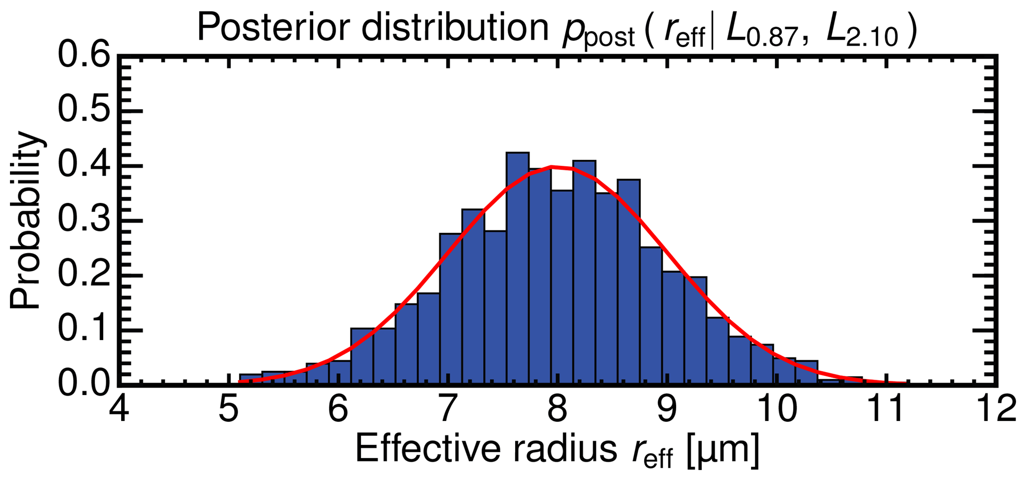
In Eq. (3), the distribution of reff in the radiative transfer ensemble is removed by the normalization with the marginal probability pfwd(reff). In the final step, the likelihood probability can be used with an arbitrary prior ppr(reff) to get the posterior probability given measurements of L0.87 and L2.10. Therefore, the arbitrary prior ppr(reff) must be included within the bounds of the marginal probability pfwd(reff) in the forward calculations. Values of reff that are not included in the forward calculations cannot be retrieved since the likelihood probability is not defined for them. For given radiance measurements L0.87 and L2.10, Fig. 1 shows an exemplary Monte Carlo approximation (blue histogram) of a posterior distribution (red line). With its mean and its standard deviation, the posterior distribution provides an estimation of the mean effective radius 〈reff〉.
2.3 Radiation transport model
The analysis of radiative transfer effects in one-dimensional clouds is done using DISORT (Stamnes et al., 1988). The representation of 3-D radiative transfer in realistic cloud ensembles is done using the Monte Carlo approach with the Monte Carlo code for the physically correct tracing of photons in cloudy atmospheres (MYSTIC; Mayer, 2009). In order to avoid confusion with the Monte Carlo sampling of posterior distributions mentioned above, this method will be termed “3-D radiative transfer forward modeling” in the following. Both codes are embedded in the radiative transfer library libRadtran (Mayer et al., 2005; Emde et al., 2016), which provides prerequisites and tools needed for the radiative transfer modeling. The atmospheric absorption is described by the representative wavelengths absorption parameterization (REPTRAN; Gasteiger et al., 2014). This parameterization is based on the HITRAN absorption database (Rothman et al., 2005) and provides spectral bands of different resolutions (1, 5, and 15 cm−1). Calculations have shown that the spectral resolution of 15 cm−1 (e.g., Δλ=1.1 nm at 870 nm, Δλ=6.6 nm at 2100 nm) best suits the spectral resolution of common hyperspectral imagers. The extraterrestrial solar spectrum is based on data from Kurucz (1994) which is averaged over 1 nm. In order to include vertical profiles of gaseous constituents, the standard summer mid-latitude profiles by Anderson et al. (1986) are used throughout this work. Since gaseous absorption is negligible at the chosen wavelength region of 870±0.6 nm and 2100±3.3 nm, this choice still allows for a tropical as well as a mid-latitude application of the retrieval. Pre-computations of the cloud scattering phase function and single scattering albedo are done using the Mie tool MIEV0 from Wiscombe (1980). When not mentioned otherwise, a gamma size distribution with α=7 was used for the Mie calculations. The high computational costs of the 3-D Monte Carlo radiative transfer method for tracing large numbers of photons are reduced using the Variance Reduction Optimal Option Method (VROOM) (Buras and Mayer, 2011), a collection of various variance reduction techniques.
2.4 Cumulus cloud model
In order to calculate realistic posterior probability distributions , likelihood probabilities, produced by a sophisticated forward model, have to be combined with a realistic prior. While Marshak et al. (2006a) used statistical models to obtain this prior of 3-D cloud fields, the physical consistency of cloud structures and cloud microphysics are an advantage of the explicit simulation of cloud dynamics and droplet interactions. Following Zinner et al. (2008), this work applies the three-dimensional radiative transfer model MYSTIC to realistic cloud fields which were generated with a large eddy simulation (LES) model on a cloud-resolving scale. While Zinner et al. (2008) use realistic cloud structures combined with a bulk microphysics parameterization, this work extends their approach by including explicit simulations of entirely consistent, spectral cloud microphysics. In order to cover clean as well as polluted atmospheric environments, LES model outputs with different CCN concentrations will be used.
Large-eddy simulations of trade-wind cumulus clouds were initially performed by Graham Feingold in the context of the Rain In Cumulus over Ocean (RICO) campaign (Rauber et al., 2007). The simulations use an adapted version of the Regional Atmospheric Modeling System (RAMS) coupled to a microphysical model (Feingold et al., 1996) and were described in more detail in Jiang and Li (2009). In addition to the high spatial resolution, cloud microphysics are explicitly represented by size-resolved simulations of droplet growth within each grid box. The cloud droplet distributions cover radii between 1.56 and 2540 µm, which are divided into 33 size bins with mass doubling between bins. All warm cloud processes, such as collision–coalescence, sedimentation, and condensation and evaporation are handled by the method of moments developed by Tzivion et al. (1987, 1989). Droplet activation is included by using the calculated supersaturation field and a given cloud condensation nucleus concentration in two versions where and . The LES simulations (dx25-100 and dx25-1000; Jiang and Li, 2009) have a domain size of 6.4 km × 6.4 km × 4 km with a spatial resolution of 10 m in the vertical and a spatial resolution of 25 m × 25 m in the horizontal with periodic boundary conditions. As initial forcing, thermodynamic profiles collected during the RICO campaign (Rauber et al., 2007) were used. With condensation starting at a cloud base temperature of around 293 K at 600 m, the cloud depth of the warm cumuli varies over a large range from 40 m to a maximum of 1700 m (Jiang and Li, 2009).
In order to sample a representative prior from these cumulus cloud simulations, a 2 h (12:00–14:00 LT) model output is sampled every 10 min for both background CCN concentrations. As input for the following radiative transfer calculations, microphysical moments are derived from the simulated cloud droplet spectra. Using Eqs. (5) to (8), effective radius reff, liquid water content LWC and total cloud droplet concentration Nd can be calculated from mass mixing ratios mi in g kg−1 and cloud droplet mixing ratios ni in kg−1 given for the 33 LES size bins:
Figure 2 shows representative fields of cloud microphysics at 12:40 LT for the case with . In Fig. 2a, the upper-left panel (a1) shows a snapshot of the liquid water path (LWP). The upper-right panel (a2) shows a north–south and (a3) shows an east–west cross section of the liquid water content field. With 1067 g m−3, the LWP maximum is found co-located with a LWC maximum of over 2 g m−3 inside the strongest convective core. The inset in (a3) contains a zoomed view of the LWC gradient at cloud edge. For the same scene, Fig. 2b provides an overview of optical thickness τ in the upper-left panel (b1). The upper-right panel (b2) shows a north–south and (b3) shows an east–west cross section of the effective radius field. In the cross sections of reff, the growth of cloud droplets with height is visible. With an overall cloud fraction of 7.6 % and a mean optical thickness τ=27 for cloudy regions with , the maximum optical thickness of τc=176 is found at the convective core as well. At the same time, the case with has a lower LWP maximum of 660 g m−3 and a lower mean cloud optical thickness of τc=11, while the cloud fraction is a little bit higher with 8.9 %.
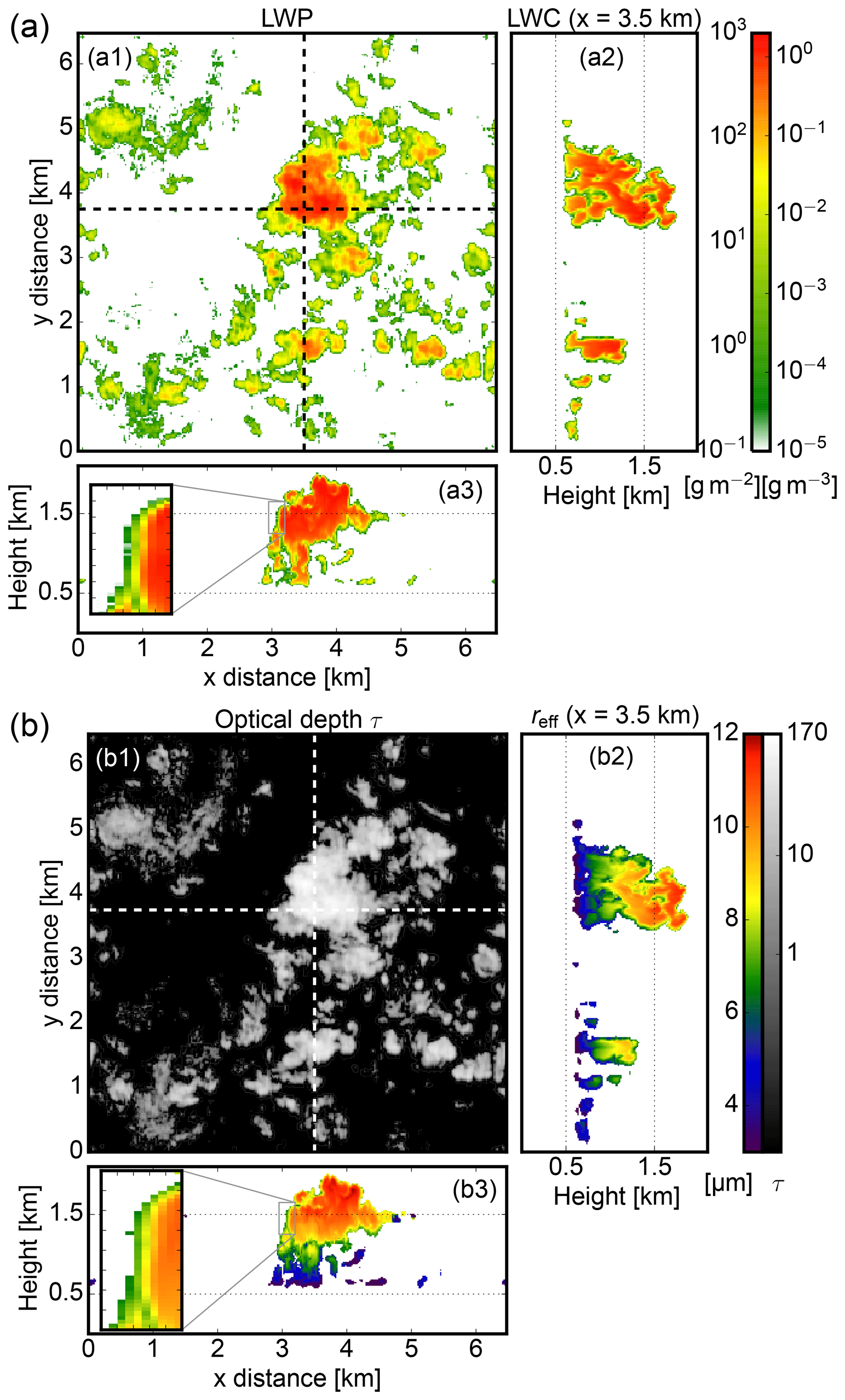
Figure 2(a) Snapshot of LES cloud fields at 12:00 LT with (a1) liquid water path in g m−3 and (a2) north–south and (a3) east–west cross sections of the liquid water content field in g m−3. (b) The same LES snapshot with (b1) optical thickness τ, as well as (b2) north–south and (b3) east–west cross sections of effective radius reff in µm. The insets in (a3) and (b3) contain zoomed cross sections of LWC and reff for a cloud edge region showing signs of lateral entrainment.

Figure 3The contoured frequency of altitude diagrams (CFADs) shows the (a) effective radius reff, (b) liquid water content LWC, and (c) cloud droplet number concentration Nd for the polluted cases with . The respective mean profile (black solid line) and its standard deviation (error bar) are superimposed. For the polluted cases with , only the mean profiles are shown (red solid lines). In both cases, the dashed profile is the theoretical adiabatic limit calculated for conditions at cloud base () and for the polluted and for the clean case.
In the following, the variation of the vertical cloud droplet growth is explored in more detail since this is the main scientific objective of the proposed retrieval. Figure 3 shows contoured frequency by altitude diagrams (CFADs; Yuter and Houze, 1995) for reff, LWC, and total cloud droplet number concentration Nd. The black lines summarize the typical profiles of reff, LWC, and Nd for , the red lines are for . The frequently occurring low values of Nd and LWC are associated with grid boxes at cloud edges while a wide spectrum of larger values are located within the cloud cores. While effective radii sharply increase from 3 µm after droplet activation at cloud base to 12 µm (for : 24 µm) at cloud top (h=1.7 km) with a small spread, the LWC increases gradually from cloud base to 0.9 g m−3 at h=1.5 km with a broad spread of LWC values. Above 1.5 km, convection is capped by a subsidence inversion where cloud liquid water accumulates to values of up to 1.5 g m−3. As intended, the two cloud ensembles cover a wide range of possible values for reff and Nd between low (“clean”) and high CCN concentration (“polluted”). Small droplet reff and slow droplet growth with height characterize cases with , while fast droplet growth to larger reff values are a characteristic of the cases with . LWC and cloud lower and upper boundaries show only small differences.
Based on the cloud base droplet number Ncb, temperature Tcb, pressure and a saturation adiabatic lapse rate (here we assume 4 K km−1), “adiabatic” reference values can be calculated for an ensemble of droplets growing by condensation during ascent, neglecting entertainment of dry environmental air (dashed lines). The existence of other effects (e.g., entrainment, coalescence) becomes evident in comparison with modeled LWC and Nd profiles, as the adiabatic theory provides only an upper limit to their values. In contrast, reff follows the adiabatic limit more closely with sub-adiabatic values between 60 and 80 %, which is in agreement with in situ aircraft observations during the RICO campaign (Arabas et al., 2009) and other studies (Martin et al., 1994).
3.1 Selection of suitable cloud sides
A key component of the Bayesian approach is the selection of a suitable sampling strategy to explore the likelihood distribution . A suitable sampling strategy becomes more essential when a computationally expensive 3-D radiative transfer method is used to sample the observation parameter space. Following Mosegaard and Tarantola (1995), the sampling of the model space should always fit the expected measurement range. Instead of sampling the radiative transfer in 3-D cloud fields at random, the intended measurement location and perspective should be taken into account.
To that end, we introduce a technique to select suitable locations within the LES model output for which cloud sides are visible from the airborne perspective. Cloud side measurements are intended for clouds within several kilometers from the instrument location. With the sun in the back, azimuthal positions of around the principal plane will be accepted for an airborne field of view, which is centered slightly below the horizon. In the following, an analytical method ensures the reproducibility through its selection of observation locations. Here, an observation kernel kFOV models the field of view with an azimuthal opening angle of and a zenithal opening angle of , centered around 5∘ below the horizon. As a function of radial distance, the observation kernel comprises a scalar weighting to curtail the desired location of clouds. In Fig. 4a, a three-dimensional visualization of the observation kernel method is presented. While the observation position (yellow dot) is moved through the model domain, the result of the convolution between observation kernel and cloud field is shown as an arbitrary score on the surface in Fig. 4a. A more detailed view of the observation kernel is given in Fig. 4b by a horizontal and in Fig. 4c by a vertical cut at the dashed cutting line. The arbitrary score is strongly negative in the vicinity of the observer to penalize locations where clouds are too close. Observation distances of 3 to 5 km turned out to maximize the likelihood of observing a complete cloud side in the used LES model output. For a distance of 2 km and onward, the weighting score becomes thus positive with a maximum at 3.5 km to favor locations with clouds in this region. For all LES cloud fields on average, this method positions the observer at a distance of around 4 km from cloud sides.
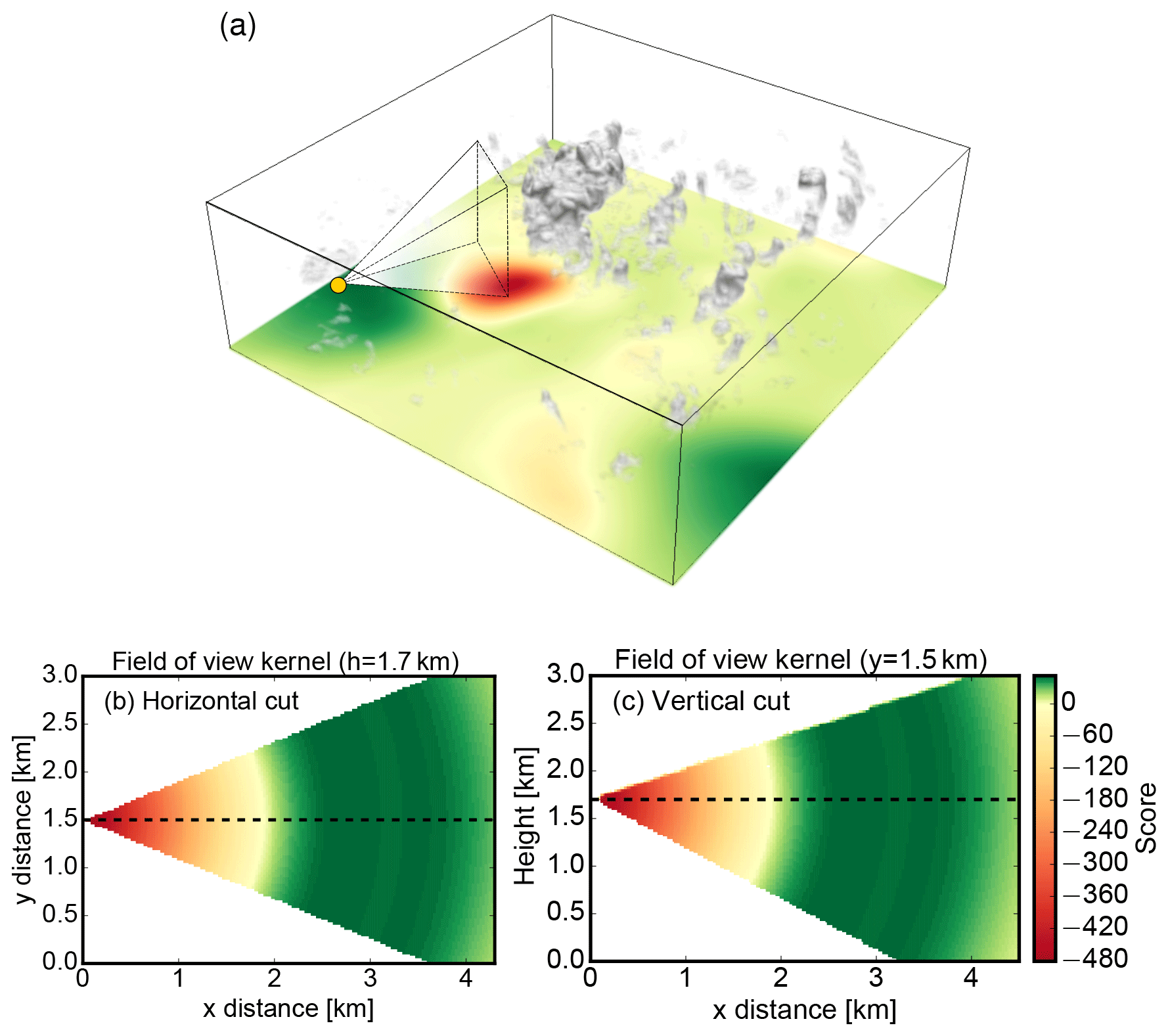
Figure 4(a) Finding the optimal observation location for cloud side measurements. The surface shows the location score derived by convolving the observation kernel (b, c) with the LES cloud field (12:40 LT) presented in Fig. 2. (b) Horizontal and (c) vertical cross sections of the observation kernel. The arbitrary score is positive for regions where clouds are desired.
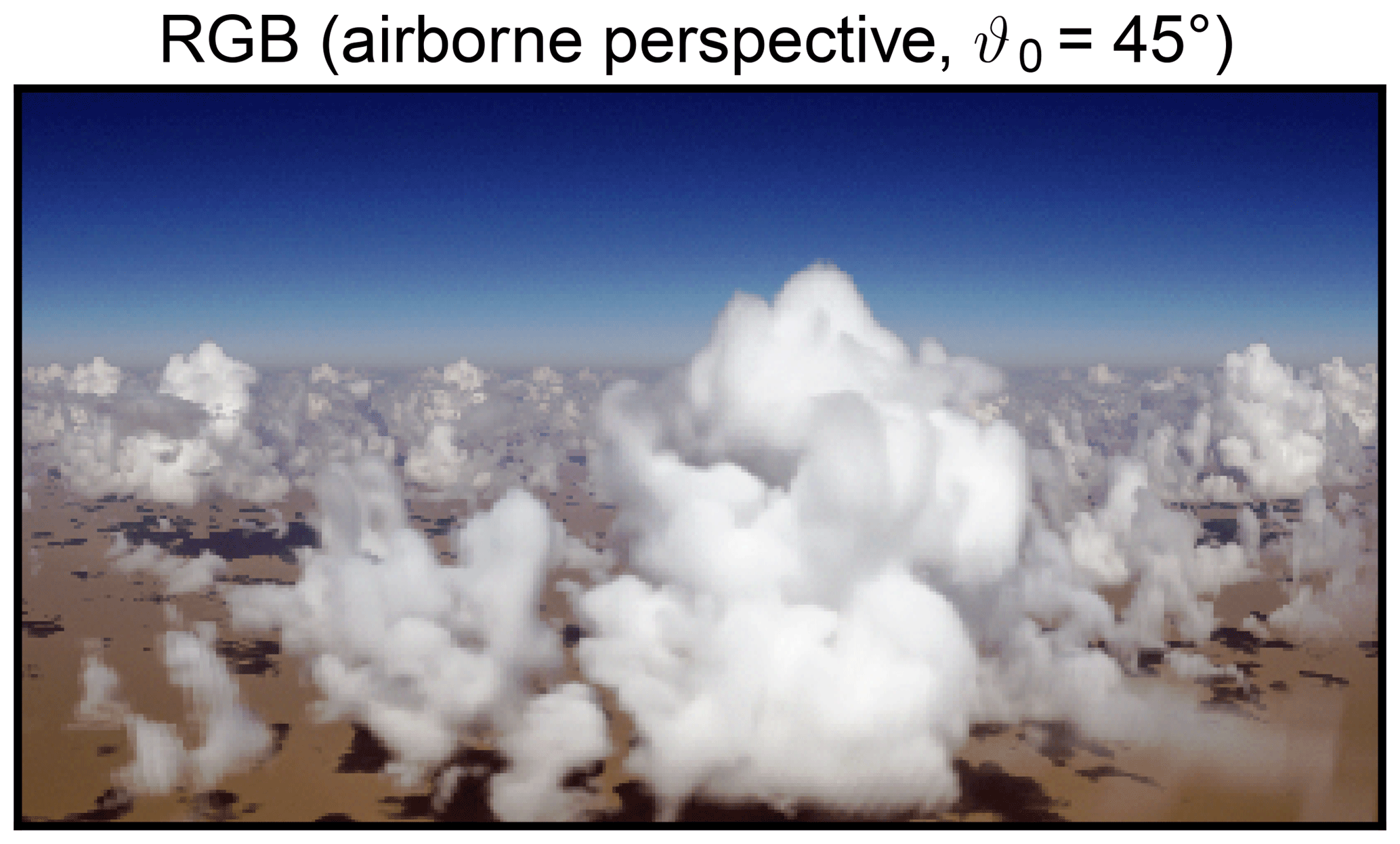
Subsequently, the field of cloudy grid boxes is convolved with the observation kernel at an observation altitude of h=1.7 km, creating a two-dimensional score field sobs. For every cloud field and chosen azimuthal orientation, the observation position is then placed where sobs has its global maximum. In Fig. 4a, the already introduced LES cloud field (12:40 LT) is shown in combination with the corresponding score field sobs obtained for a viewing azimuth of . The yellow dot indicates the observation position, where sobs has its global maximum, as recognizable by the green color. Also depicted is the field of view towards the largest cloud in the center of the domain. The red region in sobs would be unfavorable for a cloud side perspective since it would be too close to the cloud. For the selected perspective shown in Fig. 4a, a simulated true-color image is shown in Fig. 5.
3.2 Determination of the apparent effective radius
As various studies have pointed out, the process of deriving the LES variables for reff in the first place is not straightforward (Alexandrov et al., 2012; Miller et al., 2016, 2018; Zhang et al., 2017). First, reff has to be derived from model parameters which describe the particle size distribution. This step was explained in Sect. 2.4 by Eqs. (5) to (8). Secondly, an approach to infer the visible effective radius has to be developed in the case of inhomogeneous cloud microphysics. In their statistical retrieval approach, Zinner et al. (2008) traced along the line of sight of each sensor pixel until hitting the first cloudy model grid box, from which they selected their reff corresponding to the observed radiances. This method has its limitations when it comes to highly structured cloud sides with horizontally inhomogeneous microphysics. The neglect of photon penetration depth disregards reflection from deeper within the cloud. In the solar spectrum, radiance observations contain information from a multi-scattering path and not from the first grid box alone. With the line-of-sight method, the retrieved effective radius reff becomes biased towards droplet sizes found directly at cloud edges. However, due to very low LWCs, these grid boxes only have a marginal contribution to the overall reflectance.
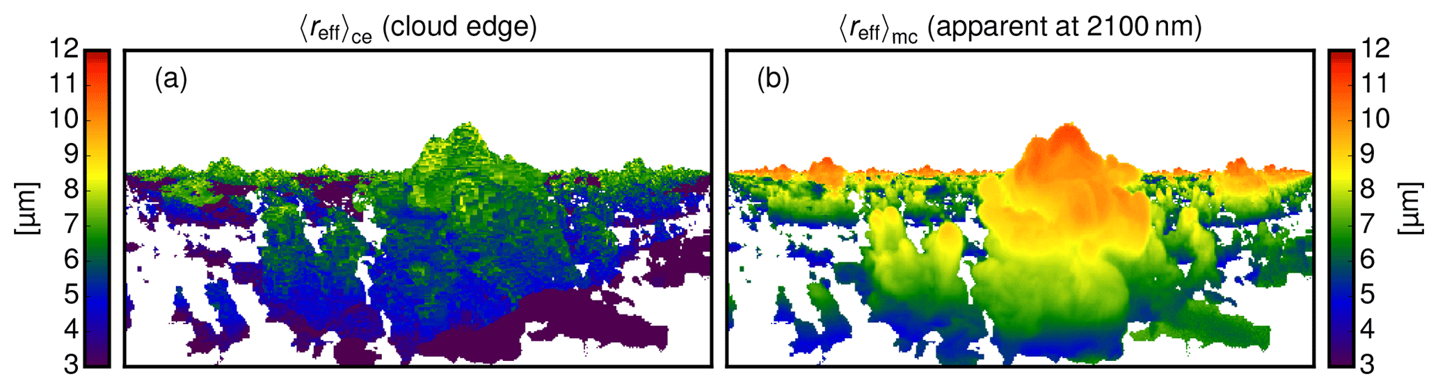
Figure 6(a) Effective radii reff found at cloud edge for the scene shown in Fig. 5, (b) apparent effective radii 〈reff〉app obtained with MYSTIC REFF for the same scene.
As Platnick (2000) showed, the penetration depth of reflected photons in the visible spectrum lies within a few hundred meters, while in the near-infrared spectrum the penetration depth is only a few dozen meters. The co-registration of responsible cloud droplet sizes with modeled radiances is essential. Besides the observation perspective, this apparent effective radius 〈reff〉app also depends on the observed wavelength since different scattering and absorption coefficients lead to different cloud penetration depths.
In the following, a technique will be introduced to obtain 〈reff〉app during the Monte Carlo tracing of photons. As discussed by Platnick (2000), there exist analytical as well as statistical methods to consider the contribution of each cloud layer to the apparent effective radius 〈reff〉app. Advancing the one-dimensional weighting procedures of Platnick (2000) and Yang et al. (2003), the 3-D tracing of photons in MYSTIC is utilized to calculate the optical properties of inhomogeneous, mixed-phase clouds. The apparent effective radius 〈reff〉ph for a photon is a weighted, linear combination of the individual effective radii reff the photon encounters on its path through the cloud:
In Eq. (9), the effective radii are weighted with the corresponding extinction coefficient kext of the cloud droplets along the path length in each grid box. Subsequently, the mean over all photons traced for one forward simulated pixel leads to the apparent effective radius 〈reff〉app of this pixel:
In Eq. (10), the photon weight wph describes the probability for the current photon path. With each absorption (or scattering) event, this weight is reduced until it reaches the detector where it is summed and converted into radiance. As the photon weights wph are also used in the calculation of L0.87 and L2.10, the apparent effective radius 〈reff〉app can be derived simultaneously. This method was integrated within the MYSTIC 3-D code and will, therefore, be referred to as the MYStic method To Infer the Cloud droplet EFFective Radius (MYSTIC REFF).
For the cloud scene shown in Fig. 5, Fig. 6b shows the apparent effective radius 〈reff〉app obtained with MYSTIC REFF. Compared with the effective radius found at the cloud edge shown in Fig. 6a, the apparent effective radius 〈reff〉app appears much smoother in Fig. 6b. The range of values for 〈reff〉app obviously compares much better with the range of values of reff shown in Figs. 2b3 and 3a. The method shows very good agreement with the analytical solution of Yang et al. (2003) for homogeneous mixed-phase clouds and Platnick (2000) for one-dimensional clouds with a vertical effective radius profile.
Reflected radiance at non-absorbing wavelengths is mainly influenced by the optical thickness and by the amount of radiation incident on the cloud surface. For the latter, the cloud surface orientation relative to the sun is decisive. Therefore, an unknown cloud surface orientation is a challenge for all retrievals using radiances to derive τc and reff (e.g., Nakajima and King, 1990). In contrast to the typical observation geometry from above, where a plane-parallel cloud is assumed, the cloud surface orientation is mostly unknown for the cloud side perspective. In such a situation, where only the scattering angle ϑs is known, the limitation to optically thicker clouds can be a solution.
4.1 Limitation to optically thicker clouds
With increasing optical thickness τc, the solar cloud reflectance becomes less sensitive to variations of τc. This reduces an essential degree of freedom with respect to the radiative transfer. By “optically thicker”, we refer to cumuli contained in the LES model output which exhibit well-developed cloud sides, e.g., like cumuli mediocris, cumuli congestus and trade-wind cumuli. To give a concrete example, this term includes clouds with τc>15, e.g., with an average LWC of 0.5 g m−3, reff=10 µm and with a vertical extent of 200 m and onward. Since the maximum optical thickness contained in the LES output is τc=176, the retrieval is designed for cumuli with τc=15–150. To dissect the impact of an unknown cloud surface orientation on the effective radius retrieval, the following study will use a “optically thick” water cloud (τc=500). We subsequently develop a method to exclude cloud shadows and to mitigate radiance ambiguities for the cumulus clouds contained in the LES ensemble using the obtained insights.
4.2 Ambiguities of reflected radiances
In the following study, the ambiguity caused by the unknown cloud surface orientation and the remaining sensitivity to the effective radius will be explored. For this idealized study, molecular absorption and scattering will be neglected. Figure 7 shows the basic geometry for cloud side remote sensing. Here, the cloud surface normal is , the illumination vector from the sun is and the viewing vector towards the observer is .
The viewing zenith angle ϑ and the sun zenith angle ϑ0 are referenced in ground frame coordinates. Corresponding to these two angles, two additional angles exist which describe the inclination of and on the oriented cloud surface: the local illumination angle and the local viewing angle ϑ* with respect to the cloud surface.
4.2.1 Principal plane (1-D)
First, all vectors are assumed to be within the principal plane (the plane spanned by and ). Figure 7 shows two different viewing angles onto a vertical cloud surface and the same local illumination angle . In the following study, global illumination and viewing geometry remain constant while the cloud surface is rotated in a clockwise direction. By varying the cloud surface normal, this approach explores the ambiguity of L0.87 and L2.10 in the context of an unknown cloud surface orientation. For the direct backscattering geometry (Fig. 7a), the local viewing angle and the local illumination angle are always equal (). In contrast, the local viewing angle can be larger or smaller () than the local illumination angle for scattering angles (Fig. 7b).

Figure 7Two observation geometries with a scattering angle of (a) and (b). The same cloud surface orientation (cloud surface normal) and illumination (solar direction vector) but different local viewing angle ϑ*. The impact of the indicated cloud surface rotation on reflected radiances is shown in Fig. 8.
For both cases, Fig. 8 shows spectral radiances L0.87 and L2.10 during the clockwise rotation of the cloud surface.
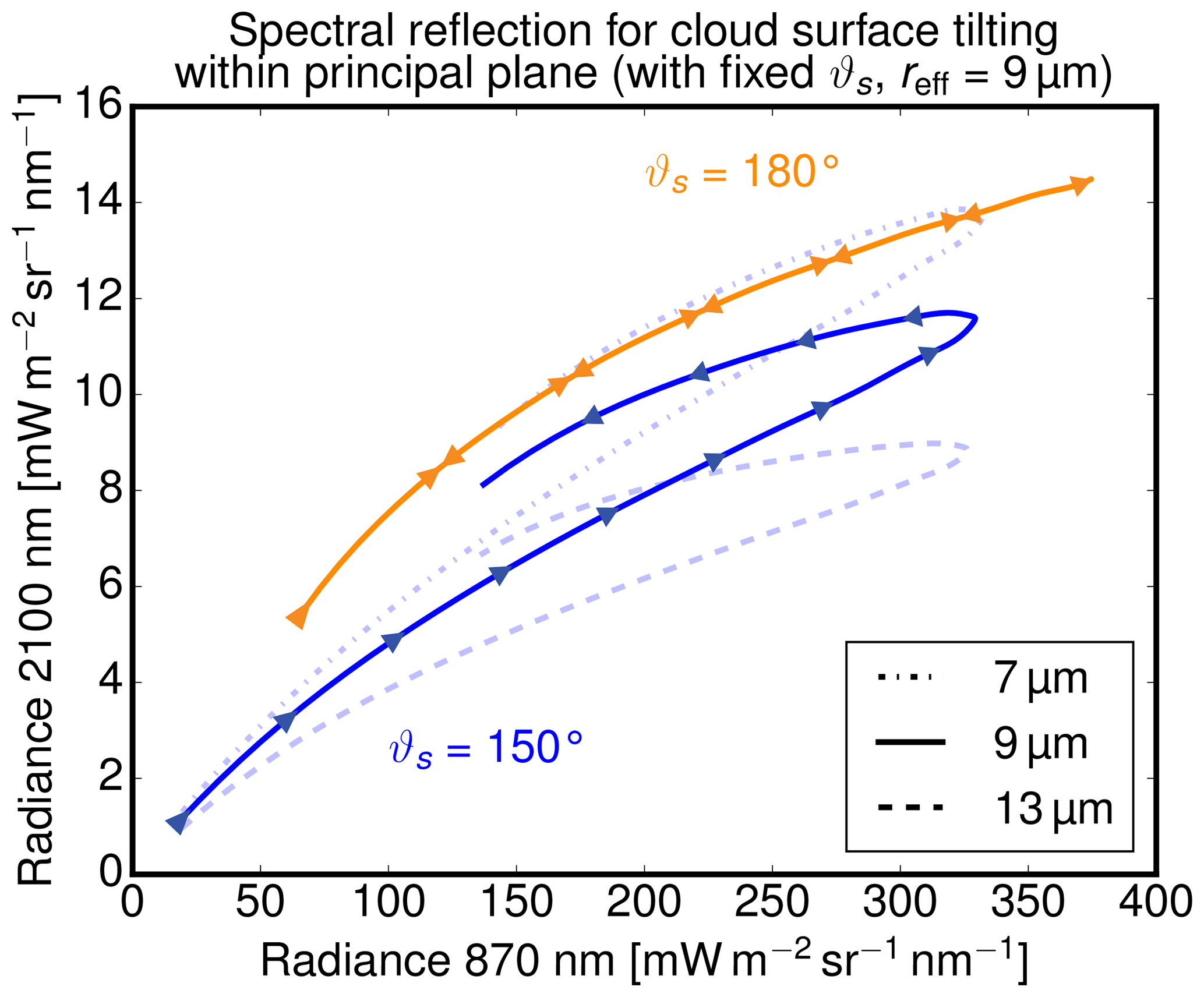
Figure 8Spectral radiances used in two-wavelength retrievals at λ=870 nm and λ=2100 nm during the rotation of the cloud surface for observation geometries shown in Fig. 7. Calculations of spectral reflection were done for an optically thick (τ=500) water cloud with a fixed effective radius reff=9 µm, a fixed scattering angle of (orange line, 9 µm), and three different effective radii with a fixed scattering angle of (blue lines, 7, 9, and 13 µm).
The radiative transfer calculations for this surface rotation of a water cloud were done with DISORT by varying the illumination and viewing angles while the scattering angle remained fixed. To exclude any effects of a varying optical thickness, the calculations were done for a very high optical thickness of τ=500 and a fixed reff=9 µm. The arrows in Fig. 8 indicate the progression of radiance values during the rotation of the cloud surface within the principal plane. The figure uses a typical two-channel diagram with the absorbing channel on the x axis and the non-absorbing on the y axis. Nakajima and King (1990) used this form to present the dependence of reflected radiance in both channels on the systematic variation of τ and reff values for plane-parallel clouds (hereafter denoted as “two-wavelength retrieval“ and “two-wavelength diagram”). The similarity of these lines to the isolines for fixed reff and varying τ in their diagrams is striking.
Numerous studies (Cahalan et al., 1994; Varnai and Marshak, 2002; Zinner and Mayer, 2006; Vant-Hull et al., 2007) pointed out that tilted and therefore more shadowed or illuminated cloud sides have a huge impact on the retrieval of optical thickness. The radiance similarity of cloud surface rotation and optical thickness variation further underlines the necessity to restrict the retrieval to optically thicker clouds (e.g., τc>15), when the cloud surface orientation is unknown. The following study will first focus on the “optically thick” water cloud (τc=500) to exclude any influence of optical thickness. In this way, the remaining information content for reff in L0.87 and L2.10 is determined.
4.2.2 Influence of scattering angle ϑs
The obvious difference in Fig. 8 between the direct backscatter case and the case with a scattering angle of highlights the influence of ϑs on the radiance ambiguity. While the radiance first increases at both wavelengths as the local illumination and viewing angle becomes smaller, it is only in case of direct backscatter that spectral radiances decrease the same way as they increased when the illumination angle becomes more oblique again. For , spectral radiances L2.10 are lower as long as when compared to the remaining part of the rotation when .
As evident in Fig. 8, a variable cloud surface orientation thus produces a characteristic bow structure outside of the direct backscatter geometry (). For the optically thick cloud (τc=500) with unknown cloud surface orientation, this bow structure introduces ambiguity between L0.87, L2.10, and different effective radii. For an oblique viewing geometry (), radiances from larger effective radii (reff=9 µm) coincide with radiances from smaller effective radii (reff=7 µm) for a steeper viewing geometry (). For brighter cloud parts, however, there remain unambiguous regions where radiance pairs of different effective radii do not overlap.
4.2.3 Origin of ambiguity for
For a deeper insight into the origin of the observed radiance ambiguity for , we analyze the angular distribution of cloud reflectance at the absorbing and non-absorbing wavelength. In the following figures, the green dot will mark the cloud surface with a steeper local viewing angle (Fig. 9, ) and the red dot the cloud surface with a more oblique local viewing angle (Fig. 9, ).
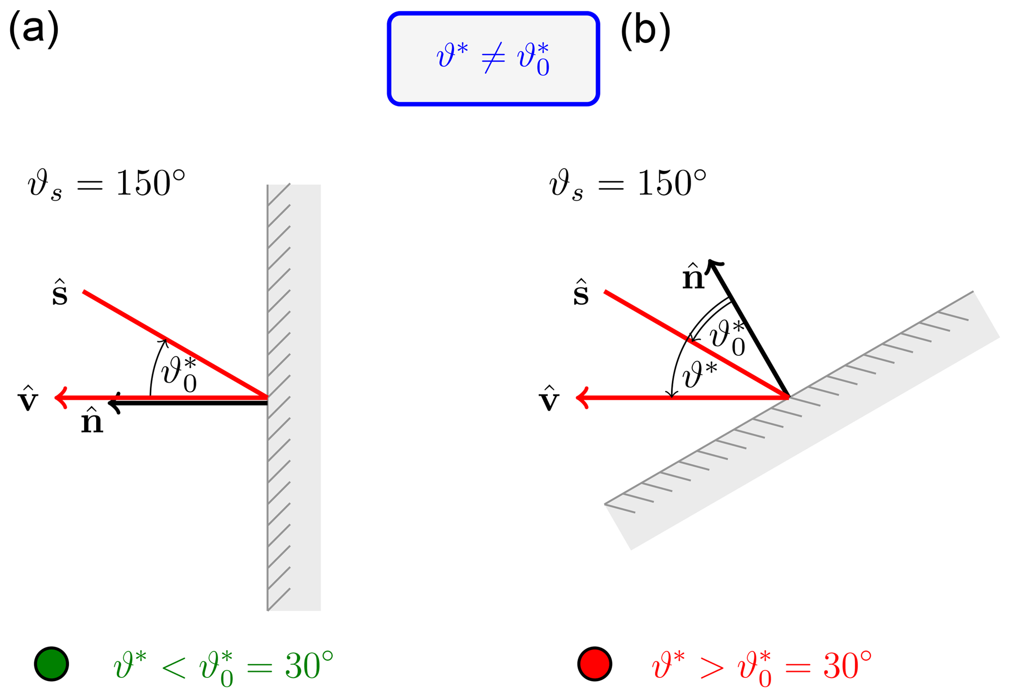
Figure 9Two observation geometries with the same scattering angle and the same local illumination angle . (a) Steep viewing direction perpendicular to the cloud surface. (b) Oblique viewing perspective .
Contrary to the last study, Fig. 10 shows radiances modeled for a fixed cloud surface orientation and illumination angle for different effective radii, while the local viewing angle ϑ* is varied.
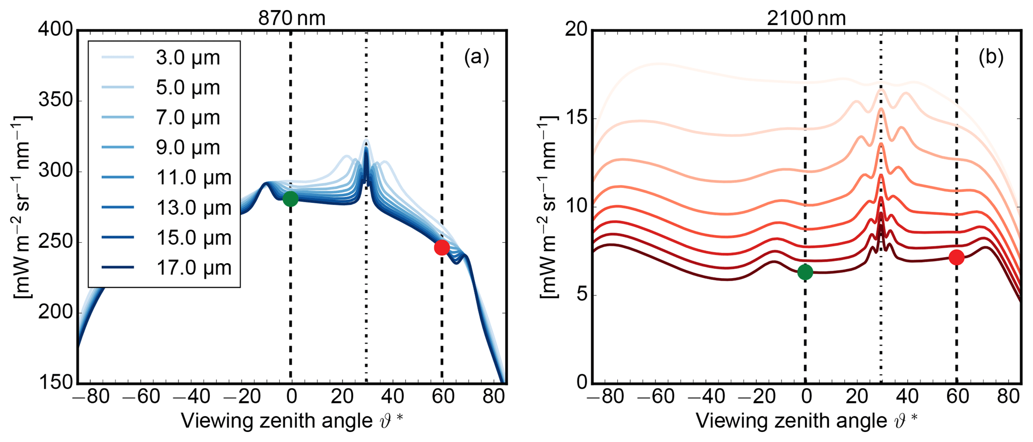
Obviously, the angular characteristic differs between the absorbing and non-absorbing wavelength. Between the steep (green dot) and the oblique (red dot) viewing perspective, the radiance at the absorbing wavelength increases slightly while the radiance at the non-absorbing wavelength decreases. This asymmetric behavior becomes less pronounced for scattering angles near . The reason for this different angular reflectance is connected with different photon penetration depths at the two wavelengths. The smaller penetration depth of near-infrared light leads to a more uniform reflection, while the larger penetration depth of visible light leads to a stronger reflection for the steep viewing perspective.
4.2.4 Spherical cloud (3-D)
Next, the analysis is extended from principal plane considerations to a full 3-D setup. To this end, 3-D MYSTIC radiance simulations were done for a spherical, optically thick water cloud (τc=500) for the different scattering regimes of and 150∘. For the direct backscatter geometry () on the left and outside the direct backscatter geometry () on the right, Fig. 11a and c show radiance images of L0.87 and Fig. 11b and d show radiance ratios L2.10∕L0.87 for the spherical water cloud. The colored radiance ratios will later help to identify regions on the sphere within the two-wavelength diagram. Furthermore, the two viewing geometries considered in Fig. 9 are marked by the green and red dots.
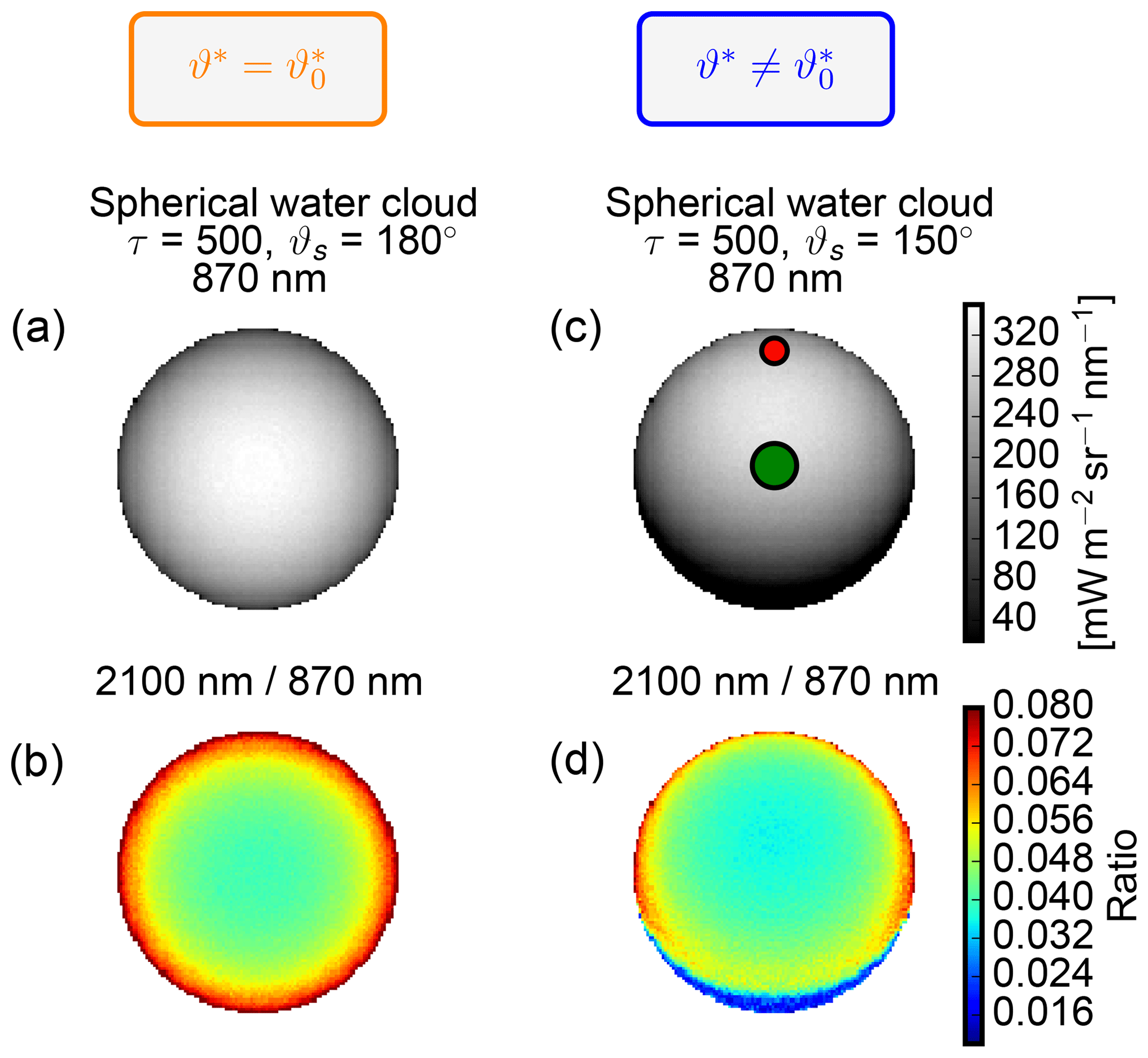
Figure 11(a, c) Images of radiance L0.87 and (b, d) of radiance ratios L2.10∕L0.87 for the spherical and optically thick water cloud (τc=500) with a fixed reff=9 µm and for a fixed scattering angle of (a, b) and (c, d). The radiance ratio is shown to identify the origin of radiance pairs in the two-wavelength diagram (Fig. 12). As previously, the green and red dots mark viewing configurations shown in Fig. 9.
Figure 12 shows the results in two-wavelength diagrams for the direct backscatter direction in Fig. 12a and for a scattering angle of 150∘ in Fig. 12b.
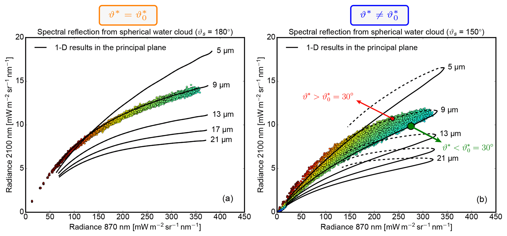
Figure 12The scatterplots show the spectral radiances at λ=870 nm and λ=2.1 µm for the spherical cloud cases with a fixed reff=9 µm. (a) Results from Fig. 11a for a fixed scattering angle of and (b) from Fig. 11c for . The color of the scatter points can be used to identify their location on the spherical water cloud in Fig. 11b and d. For the same scattering angles and analogous to Fig. 8, the black isolines show radiances from 1-D DISORT simulations for an optically thick water cloud (τc=500) with different effective radii and variable cloud surface orientation. As previously, the green and red dots mark viewing configurations shown in Fig. 9.
In the two-wavelength diagrams, the radiance pairs from the 3-D MYSTIC simulation are shown as scattered points; the results from the one-dimensional DISORT simulations for different effective radii are shown as black lines. Just like in Figs. 9 to 11, the large green and red dots in Fig. 12 indicate cloud surfaces with the same local illumination angle , but steeper (, green dot) or more oblique local viewing angle (, red dot).
This ratio reflects the radial symmetry of the local illumination angle for (Fig. 12a). For the direct backscatter geometry in Fig. 12a, 3-D results for reff=9 µm match the 1-D DISORT results for reff=9 µm very closely. Due to the radial symmetry of the local illumination angles, radiance values also decrease in a radially symmetric way with more oblique cloud surfaces. Albeit restricted to airborne or spaceborne platforms, this perspective minimizes the 3-D effect on radiance ambiguities caused by unknown cloud surface orientations. The picture changes when the observer leaves the backscatter geometry as shown for a scattering angle of in Fig. 12b. As already shown with the DISORT results in Fig. 8, the radiance pairs form a bow-like pattern with higher L2.10 values at more oblique surface orientations. Furthermore, the red and green dots with the same local illumination angle now become separated since . While radiance at the non-absorbing wavelength drops considerably with a more oblique local viewing angle (, red dot), radiance at the absorbing wavelength even slightly increases. Consequently, droplets at the red dot with reff=9 µm could be misinterpreted as effective radius reff=7 or even 5 µm .
Previous studies, like Marshak et al. (2006a) and Zinner et al. (2008), did not investigate in detail the origin of these radiance ambiguities. Nonetheless, they suggested to limit the influence of missing geometry information by additional consideration of vertical thermal radiation temperature gradients (containing part of the geometry information). In the following, a more systematic use of available geometry information in the visible and near-infrared spectrum is presented.
4.3 Additional information from surrounding pixels
Here, a technique is presented that uses information from surrounding pixels to resolve the radiance ambiguities caused by an unknown cloud surface orientation. Already Varnai and Marshak (2003) discussed and developed a method to determine how the surrounding of a cloud pixel influences the pixel brightness. In a recent study, Okamura et al. (2017) also used surrounding pixels to train a neural network to retrieve cloud optical properties more reliably. Our study will try to find a link between the pixel surrounding and the radiance ambiguity discussed in the preceding section.
As discussed in the preceding section, ambiguous radiances are caused by the asymmetric behavior of L0.87 and L2.10 when changing from a steep local viewing angle towards a more oblique perspective onto a cloud surface. While the pixel brightness L0.87 decreases considerably at a more oblique perspective, the pixel brightness L2.10 increases. While changes in L2.10 along a whole cloud profile are associated with a change in effective radius, the geometry-based brightness increase in L2.10 should generally occur at smaller scales associated with cloud structures. The method should therefore determine if the surrounding pixels are darker or brighter at λ=2100 nm. At the same time, the method should be insensitive to instrument noise or Monte Carlo noise between adjacent pixels.
4.3.1 Comparison of pixel brightness
To this end, a 2-D difference of Gaussian (DoG) filter is used to classify the viewing geometry onto the cloud surface in simulated as well as in measured radiance images. As a 2-D difference filter, it compares the brightness of each pixel with the brightness of other pixels in the periphery. The filter consists of two 2-D Gaussian functions and with different standard deviations σL and σH, which specify the inner and outer search radius for the pixel brightness comparison.
Figure 13a shows the two Gaussians as a function of the angular distance from the considered pixel within the field of view.
When the broader kernel is subtracted from the narrower kernel (Fig. 13a, black line), the average pixel brightness within σL is compared with the average pixel brightness of the center pixels within σH. This pixel brightness deviation is obtained by convolving the difference of with the radiance image L2.10.
Due to this subtraction, pixels are classified according to their positive or negative radiance deviation compared to their surrounding pixels. By using a not-too-small σH, not only the current pixel but a small surrounding is used, making the method less sensitive to noise of image sensors or Monte Carlo radiative transfer calculations.
For classification into steep or oblique perspectives, we are interested in the brightness deviation relative to the pixel surrounding it. However, the absolute pixel brightness deviation can vary from scene to scene. To ease the binning of the gradient classifier gclass(x,y), we constrain it into a fixed interval using the arctangent function:
This restriction of gclass to the range is shown in Fig. 13b, where positive values indicate pixels which are brighter at λ=2100 nm compared to the brightness of their surrounding.

Figure 13(a) 2-D difference of Gaussians (red) and (green) which is used as a filter to derive (b). The gradient classifier gclass which compares the pixel brightness with the brightness of the surrounding pixels.
4.3.2 Pixel brightness deviation as a proxy of 3-D effects
In practice, the radiance ambiguity cannot be directly derived from passive radiance measurements without a detailed knowledge of the cloud surface orientation. Hence, the following study will investigate if the gradient classifier gclass can be used as a proxy to resolve the discussed radiance ambiguity. To demonstrate the method, the cloud field illustrated in Fig. 6 was used again for radiance calculations, but with a fixed effective radius of reff=8 µm. For this fixed effective radius, the broad radiance distribution of L0.87 and L2.10 shown in Fig. 14a is mainly caused by the different cloud surface orientations discussed in the previous section. In order to identify the regions leading to the upper part of the radiance scatter cloud in Fig. 14a, an exponential function was fitted (black line) to the data points to determine the positive (red) or negative (green) deviation ΔL2.10 from the best fit (black line) for each radiance pair.
In the following, this deviation ΔL2.10 is taken as a reference for a perfect separation of 3-D radiance ambiguities. It is important to mention that this deviation ΔL2.10 can only be determined when the effective radius is already known. A method that would yield a similar separation without prior knowledge of reff could be used as a proxy to mitigate the problem of ambiguous radiances.
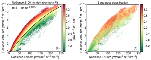
Figure 14(a) Two-wavelength diagram for the MYSTIC calculation shown in Fig. 5 but with a fixed effective radius of reff=8 µm. (b) Result of the gradient classifier gclass applied to the same scene.
First, an optimal inner and outer search radius σH and σL has to be found to use gclass as a proxy for the inaccessible radiance deviation ΔL2.10. This optimal search region was found by variation of search radii σH and σL and subsequent correlation of gclass (shown in Fig. 15b) with the radiance deviation ΔL2.10 (shown in Fig. 15a). A maximum correlation with ΔL2.10 was found when the filter operated between and . In spatial terms, the brightness within a search region of 30 to 150 m is compared with the considered pixel brightness. For the optimal search radii, Fig. 14 compares the radiance separation provided by the gradient classifier in Fig. 14b with the reference in Fig. 14a. Figure 15 also shows the reference and proxy as images, where the radiance deviation ΔL2.10 is shown on the left in Fig. 15a and the gradient classifier on the right in Fig. 15b.
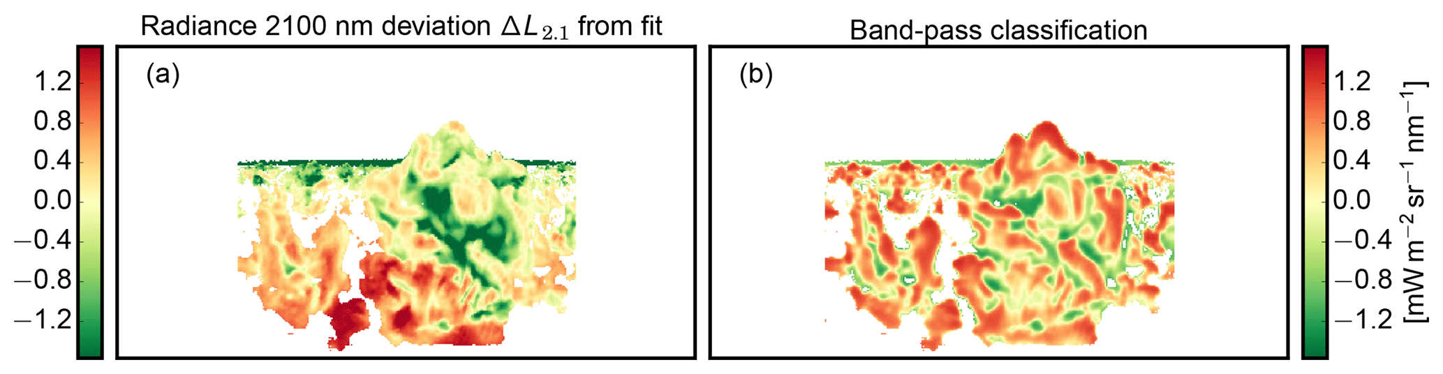
Figure 15(a) Deviation ΔL2.10 from the fit in the two-wavelength diagram in Fig. 14a used as a reference for the (b) gradient classifier gclass, which puts the pixel radiance into context with surrounding pixels.
Apparently, the radiance separation by the gradient classifier gclass is similar to the radiance deviation ΔL2.10. It is able to separate the radiance distribution into positive and negative radiance deviations ΔL2.10 at high as well as at low radiances. Large gclass values are more likely to be associated with a more oblique local viewing angle (), while smaller values are more likely to be associated with a more steep local viewing angle (). For two pixels with the same illumination angle, gclass>0 thus marks the upper radiance branch in Fig. 14b, while gclass<0 marks the lower radiance branch. Based on this feature, the gradient classifier gclass can be used as a proxy to determine the geometry-induced radiance deviation of a pixel within the radiance distribution. For the retrieval, the gradient classifier gclass is used for the 3-D forward calculation ensemble as well as for real measurements.
4.4 Exclusion of cloud shadows
Cloud regions can also be self-shadowed if the local solar zenith angle onto the cloud surface is larger than 90∘. Illuminated cloud parts can also cast shadows onto other cloud parts. Without direct illumination, reflected photons from these shadowed cloud parts originate from previous scattering events and are affected by those. For this reason, shadowed cloud parts have to be filtered out before applying any retrieval based on direct illumination.
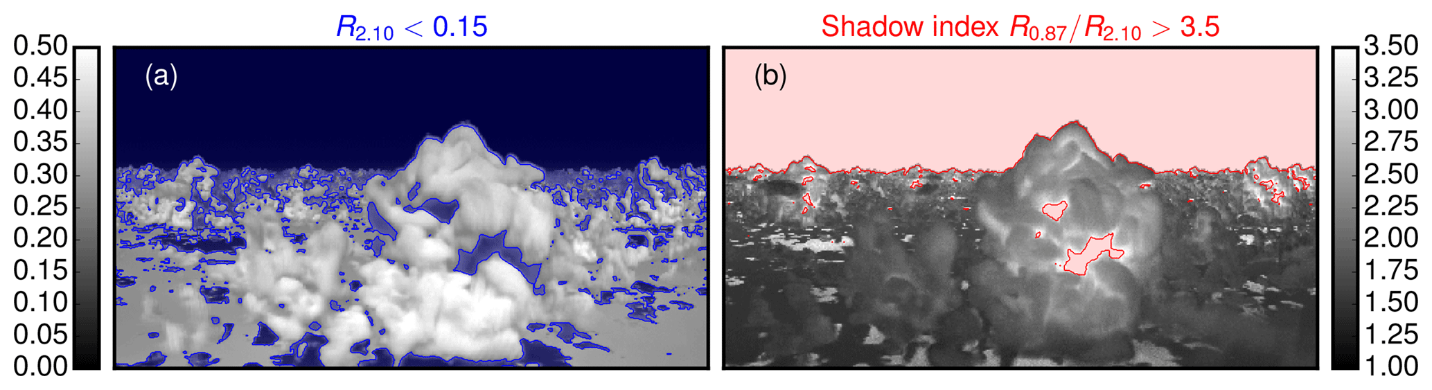
Figure 16(a) Reflectivity at 2.1 µm for the cloud scene shown in Fig. 6 (blue regions mark the simple reflectivity threshold R2.10<0.15). (b) Shadow index R0.87∕R2.10 highlighting regions of enhanced cloud absorption caused by multiple diffuse reflections (red regions mark the shadow index threshold ).
Usually radiation from shadow regions encountered more absorption compared to directly reflected light (Vant-Hull et al., 2007). This enhanced absorption is visible in Fig. 16a, where the reflectivity at 2.1 µm drops considerably for shadowed cloud regions. In Fig. 16a, the blue areas illustrate a simple reflectivity threshold R2.10<0.15. As a proxy of enhanced absorption, the reflectivity ratio R0.87∕R2.10 (Fig. 16b) increases in this regions. In the following, this ratio will be used as shadow index R0.87∕R2.10 to exclude pixels for which light has likely undergone multiple diffuse reflections:
In Fig. 16b, the red areas marks regions with . The manual inspection of many cloud scenes confirmed 3.5 as a viable shadow index threshold.
Unfortunately, clouds with very large cloud droplets (reff>12 µm) can exhibit similarly high values of the shadow index. To study this limitation, DISORT calculations were done for an idealized water cloud to characterize the shadow index with respect to cloud optical thickness and effective radius.
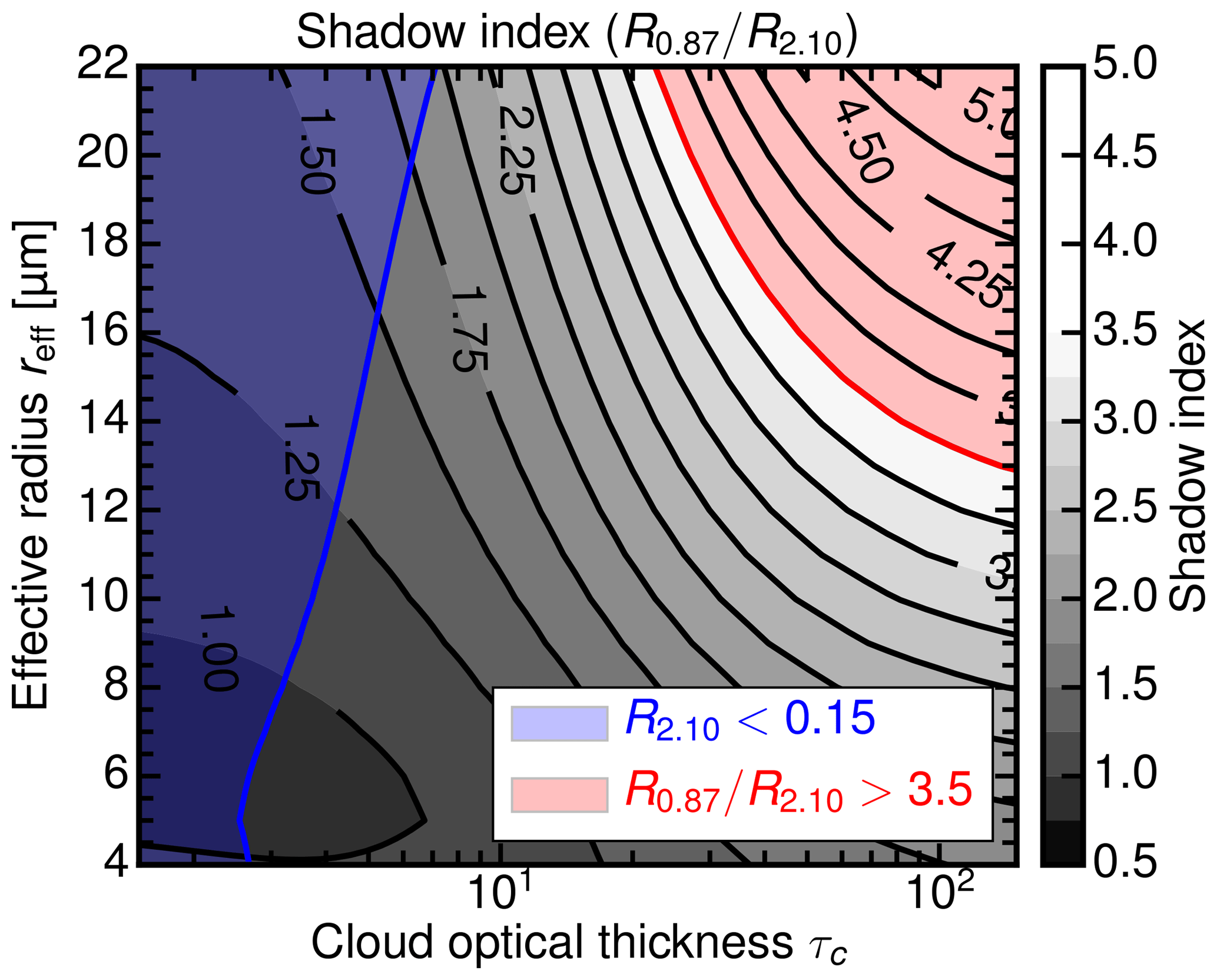
Figure 17Shadow index R0.87∕R2.10 for water clouds as a function of effective radius reff and cloud optical thickness τc for the geometry (, ), with high absorption at 2.1 µm. Like in Fig. 16, the blue area indicates the simple reflectivity threshold R2.10<0.15 while the red area indicates the shadow index threshold .
Figure 17 shows the shadow index as a function of effective radius reff and optical thickness τc for the geometry (, ), with high absorption at 2.1 µm. Like in Fig. 16, the blue area indicates the simple reflectivity threshold R2.10<0.15 while the red area indicates the shadow index threshold . Obviously, both shadow thresholds have their disadvantages. At higher optical thickness (τc>100), the shadow index can confuse very large cloud droplets (reff>12 µm) with cloud shadows. In contrast, the simple reflectivity threshold R2.10<0.15 can misidentify optically thin clouds (τc<10) as cloud shadows. The combined shadow mask fshad of both thresholds in Eq. (16) compensates for the disadvantage of the shadow index threshold:
In this way, only dark and highly absorptive cloud regions at 2.10 nm are classified as shadows. In addition, a threshold of is used to focus the retrieval on optically thicker clouds and to filter out clear-sky regions.
In this section, the Monte Carlo sampled posterior distributions will be used to infer droplet size profiles from convective cloud sides. As mentioned in Sect. 2.2, the posterior can be derived from Bayes' theorem by solving the easier forward problem for all values of reff.
The three-dimensional radiative transfer code MYSTIC is applied to LES model clouds to obtain simulations of realistic specMACS measurements. A whole ensemble of these MYSTIC forward simulations of cloud sides will then be incorporated within the statistical framework introduced in Sect. 2.1. Subsequently, the sampled statistics of reflected radiances are analyzed for their sensitivity to the effective cloud droplet radius.
5.1 Implementation of the 3-D forward radiative transfer ensemble
In the following, an ensemble of 3-D radiative transfer simulations is created to sample the posterior probability distribution . The ensemble of simulated cloud side measurements is set up by using the method to select suitable observation perspectives introduced in Sect. 3.1. During the radiative transfer calculations, the MYSTIC REFF method (Sect. 3.2) determines the apparent effective radius which links the simulated radiances with the corresponding cloud droplet sizes. Despite the variance reduction methods in the MYSTIC code itself (Buras and Mayer, 2011), the time-consuming 3-D technique still limits the number of model runs. Figure 18 illustrates the different illumination setups and the viewing geometry included within the 3-D forward simulation ensemble. With LES cloud tops between 1.5 and 2.0 km, the airborne perspective is set to an altitude of h=1.7 km. Since the retrieval should also be applicable in tropical regions, solar zenith angles were chosen at ϑ0=7, 27, 47 and 67∘.
For each observation position selected in Sect. 3.1, images of cloud sides were simulated using MYSTIC. In line with the position selection method, the field of view of each image has an azimuthal opening angle of , a zenithal opening angle of and is centered around 5∘ below the horizon. Comprising 720 × 368 pixels, each image was calculated with a spatial resolution of 0.125∘. For this image setup, solar radiances were calculated at the non-absorbing wavelength λ=870 nm (L0.87) and the absorbing wavelength λ=2100 nm (L2.10). Since the width of the cloud droplet size distribution has no large impact on radiances at L0.87 and L2.10 (analysis not shown), the scattering properties were derived according to Mie theory using modified gamma size distributions with a fixed width of α = 7 and the effective radius as simulated by RAMS. For the ensemble, the surface albedo was set to zero since the influence of radiation reflected by vegetation on the ground is masked in the measurements. This technique will be described in the following Part 2 of this paper.
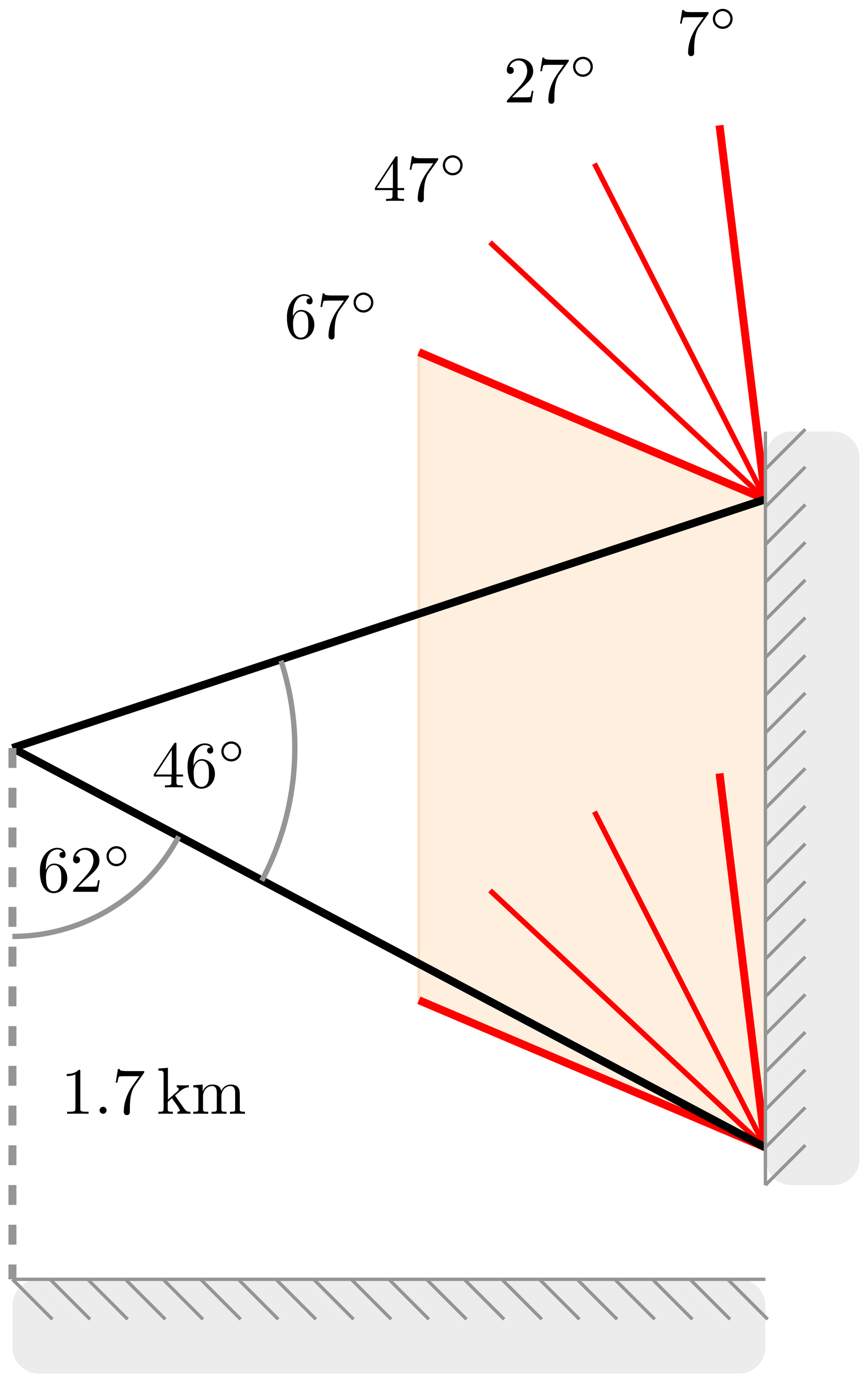
Figure 18Setup of the viewing geometry (, starting 62∘ from nadir) and the illumination geometry (ϑ0=7, 27, 47 and 67∘) for the airborne (h=1.7 km) 3-D forward simulation ensemble. The horizontal extent of the field of view is from the principal plane.
Atmospheric aerosol was included by using the continental average mixture from the Optical Properties of Aerosols and Clouds (OPAC) package (Hess et al., 1998). The aerosol optical thickness (AOT) at 550 nm is around for this profile. This aerosol profile is typical for anthropogenically influenced continental areas and contains soot and an increased amount of insoluble (e.g., soil) as well as water-soluble (e.g., sulfates, nitrates and organic) components.
A compromise had to be found to minimize the noise of the 3-D Monte Carlo radiative transfer results and to keep computation time within reasonable limits. Here, the Monte Carlo noise should stay below the accuracy of the radiometric sensor which is assumed to be ∼5 %. The photon number was thus chosen to be 2000 photons per pixel, which leads to a standard deviation of about 2 %.
All 12 RICO LES snapshots between 12:00 LT (local time) and 14:00 LT with a time step of 10 min were included in the 3-D forward simulation ensemble. For four azimuth directions φ=45, 135, 225, and 315∘, suitable locations for cloud side observations were determined in each LES snapshot. For the polluted as well as for the clean cloud ensemble, cloud scenes have been simulated for four solar zenith angles and two wavelengths with 720×368 pixels, totaling 101 744 640 forward simulation pixels. In total, 2×10¹¹ photons have been traced on a computing cluster with 300 cores consuming 2×10⁸ s of CPU time.
5.2 Construction of the lookup table
In the next step, simulated radiances were binned into a multidimensional histogram with equidistant steps in , and gclass. Here, it is important to emphasize that the retrieval is designed to be independent of a priori knowledge of NCCN. If the posterior distributions are separated between clean and polluted cases, the retrieval can tend to larger reff when a low NCCN is measured. Such a retrieval would be unsuitable to study aerosol–cloud interactions. For this reason, the radiance results from the polluted and the clean cloud ensemble are combined within the same histogram. Table 1 shows the specific binning of this histogram.
Table 1Variables, range, and step size into which simulated radiances are binned to obtain a multidimensional histogram which is then used as a lookup table.

a b µm.
During this discretization, radiances were counted in adjoining bins by linear interpolation. In the following, the histogram will be normalized to yield the posterior probability .
5.3 Biased and unbiased priors
In the used cloud fields, the effective radius always increases with height which might impact the retrieval. The retrieval should not exhibit any trend towards a specific profile. Otherwise, the retrieval would reflect a priori knowledge about the vertical profile of cloud microphysics. For this reason, the assumed prior is a key element to be considered in the sampling of the posterior and the subsequent Bayesian inference. In the case of cloud side remote sensing, two possible priors ppr(reff) come into mind: a uniform prior or the LES model provided prior. For the LES model the prior is a function of viewing geometry, as some reff are more likely to be observed under certain viewing directions. In particular, relative frequency of reff for different scattering angles ϑs and gradient classes should be the same. For aerosol–cloud interaction studies, the prior probability for reff should be uniform to avoid the introduction of a model bias.
Another important prerequisite of the Monte Carlo-based Bayesian approach is the sufficient sampling of the likelihood probability . Naturally, effective radii not included in the ensemble of forward calculations cannot be retrieved using Bayesian inference. Furthermore, it should be kept in mind that sparsely sampled likelihood regions are probably not representative for the whole distribution. This is especially true for the smallest and largest effective radii contained in the LES model.
For these reasons an unbiased coverage of the likelihood probability is sought. To this end, the ensemble with the normal cloud microphysics data from the LES model was complemented with calculations with vertically flipped cloud microphysics. The flipped cloud microphysics were derived by taking the additive inverse of the original effective radius fields and add an offset :
To ensure positive and realistic values for , the offset was chosen to be at least 4 µm larger than the largest values found in all cloud fields. Thus, was used in Eq. (17) for the polluted cloud ensemble and for the clean cloud ensemble . To preserve the optical thickness τorig of the original cloud field,
the well established relationship in Eq. (19) was used to derive the liquid water content LWCflip for the flipped cases in Eq. (20):
5.4 Radiance and posterior distributions
The following section will present the radiance histograms and the corresponding posterior distributions . Analogous to the likelihood distribution, the first gives the spread of radiances for a given effective radius reff, while the latter describes the spread of effective radii reff for a given radiance pair L0.87 and L2.10. Figure 19a shows a 2-D histogram of simulated radiance combinations L0.87 and L2.10 for the airborne perspective. The histogram shows the results for the effective radius bin centered at reff=10 µm, the scattering angle bin between ϑs=130 and 140∘ and the gradient class bin gclass=4 which holds pixels that are brighter as their surroundings. The radiance spread from the three-dimensional model cloud sides, for the most part, can be explained by the one-dimensional DISORT results for τc=500 (dashed line for variable cloud surface inclination).
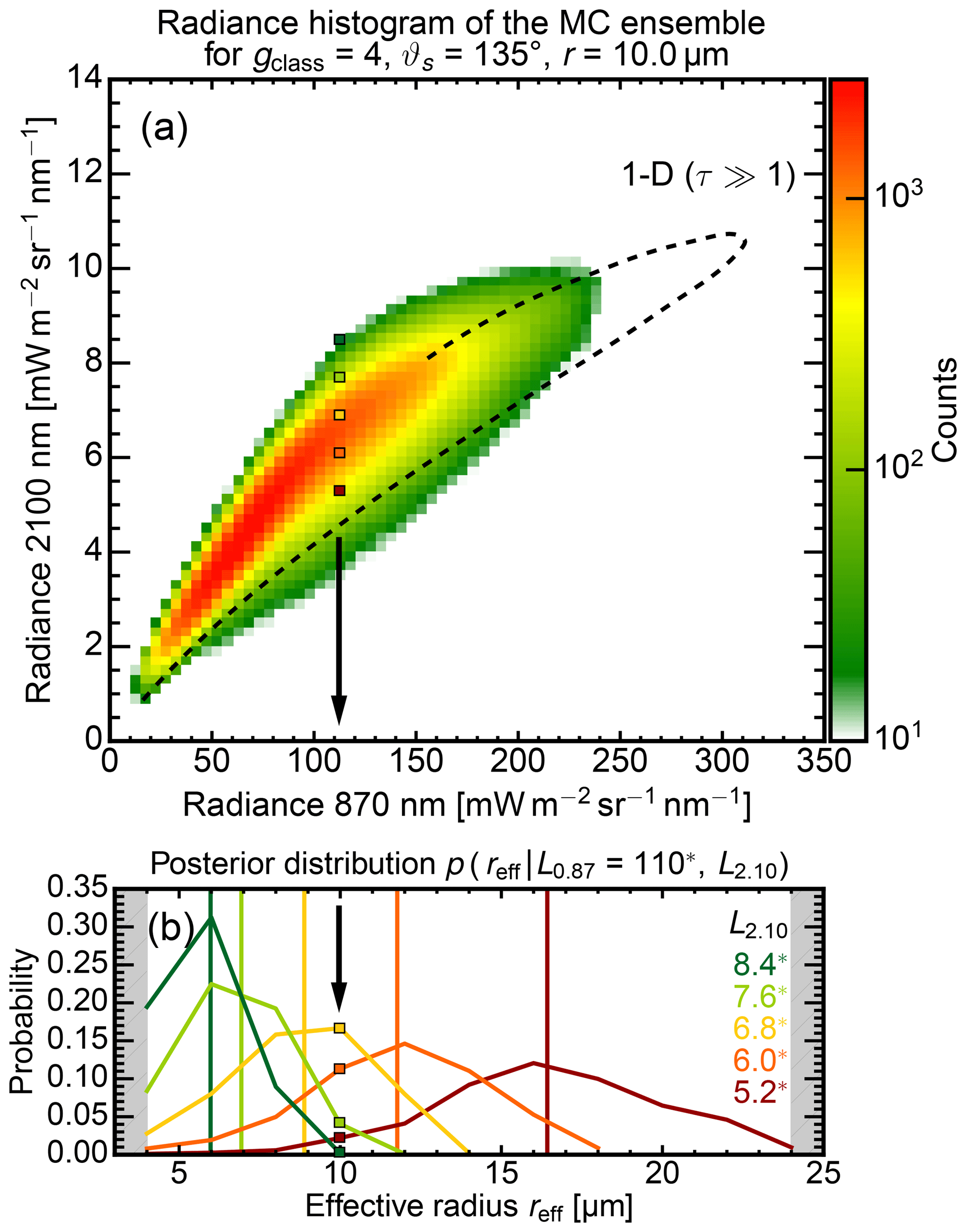
Figure 19(a) Radiance histogram (, gclass=4) for the 3-D forward simulation ensemble of cloud sides, which illustrates the radiance spread for the effective radius bin of reff=10 µm. The dashed line shows reflected radiances which were calculated with DISORT (1-D RT code) for an optically thick (τc=500) water cloud with a variable cloud surface inclination within the principal plane. The colored dots indicate locations within the histogram for which the posterior distributions are shown in Fig. 19b. (b) Corresponding posterior probability for a fixed radiance at the non-absorbing wavelength and different L2.10 radiances at the absorbing wavelength. The vertical lines indicate the corresponding mean effective radius for each posterior distribution.
After normalization of the histograms in Eq. (3) and after the application of the uniform prior in Eq. (4), the posterior probabilities can be examined. Figure 19b shows posterior probabilities as a function of reff for different radiances L2.10 at the absorbing wavelength corresponding to the colored dots in the histogram panel (Fig. 19a). The vertical lines indicate the corresponding mean effective radius for each posterior distribution which were derived using Eq. (21). The descending order of mean effective radii with ascending radiance L2.10 demonstrates the general feasibility to discriminate different effective radii in cloud side measurements. Albeit a relatively large statistical retrieval uncertainty σ(reff), the measurement of a radiance pair (L0.87, L2.10) can still narrow down reff to ±1.5 µm around the most likely value. Interestingly, σ(reff) increases with the effective radius from to . In the following, the tabulated set of posterior distributions is used as a lookup table for the effective radius retrieval.
5.5 Bayesian inference of the effective radius
Based on this lookup table of posterior probabilities , the actual retrieval of effective radii can now be introduced. After a set of spectral radiance pairs L0.87 and L2.10 has been measured, the DoG filter (Sect. 4.3) is applied to the L2.10 image to derive the gradient classifier gclass. Scattering angles are calculated from the orientation and navigation data of the aircraft. With the four parameters, L0.87, L2.10, gclass, and ϑs defined for each pixel, the corresponding posterior is retrieved from the lookup table by linear interpolation between posteriors defined at the bin centers of the lookup table. Finally, the mean effective radius 〈reff〉 and the corresponding standard deviation σ(reff) can be derived as first and second moments of the posterior distribution:
This 1σ standard deviation σ(reff) in Eq. (22) will be referred to as the statistical retrieval uncertainty.
The next section will examine the stability of the statistical relationship between reflected radiance and cloud droplet size. How well can we retrieve the cloud droplet size after different viewing directions and cloud surface orientations have been combined within one lookup table? To answer this, the statistical retrieval is applied to simulated cloud side measurements for which the underlying effective radius is known. First, this is done for scenes that have already been included in the lookup table. Using scenes with normal and flipped effective radius profile, the lookup table is tested for an inherent bias towards a specific effective radius profile that could be caused by the chosen forward sampling strategy. In addition, tests are repeated for the same scenes with a fixed effective radius of 8 µm, a case which is not included in the lookup table.
6.1 Analysis of the sampling bias
By design, the retrieval should not exhibit any trend towards a specific profile. The polluted scene (), already introduced in Fig. 5, will be used as a first case study. Figure 20 shows the result of the statistical effective radius retrieval with the normal effective radius profile on top, the flipped profile in the center, and a fixed effective radius profile at the bottom. The retrieved mean effective radius is shown in the right panels (Fig. 20c, f, i), and the apparent effective radius 〈reff〉app is shown in the left panels (Fig. 20a, d, g). The center panels compare the mean vertical profile (lines) and its spatial standard deviation (shaded areas) of the apparent (black) and the retrieved (green) effective radius. Furthermore, the red error bars show the mean statistical retrieval uncertainty σ(reff) provided by the retrieval.
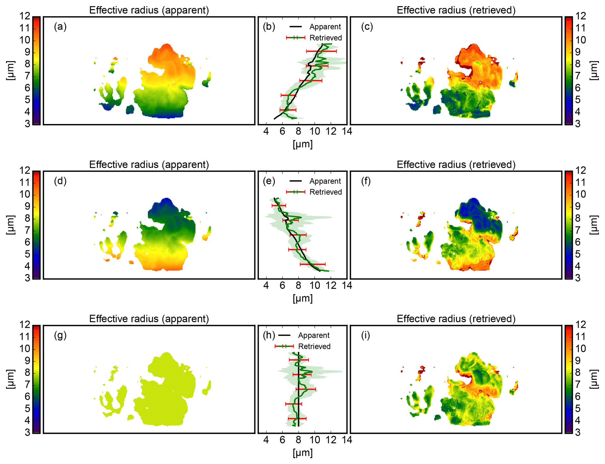
Figure 20Retrieval test between the apparent effective radius (a, d, g) and the retrieved mean effective radius (c, f, i) for the normal (a–c), flipped (d–f), and fixed (g–i) effective radius profile. (a) Apparent effective radius 〈reff〉app for the normal profile, (b) mean and standard deviation of the apparent (black) and retrieved (green) vertical effective radius profile (normal) with the mean statistical retrieval uncertainty (red error bars). (c) Retrieved mean effective radius for the normal microphysical profile, (d, e, f) As in (a–c) but for the flipped microphysical profile. (g, h, i) As in (a–c) but for the fixed microphysical profile.
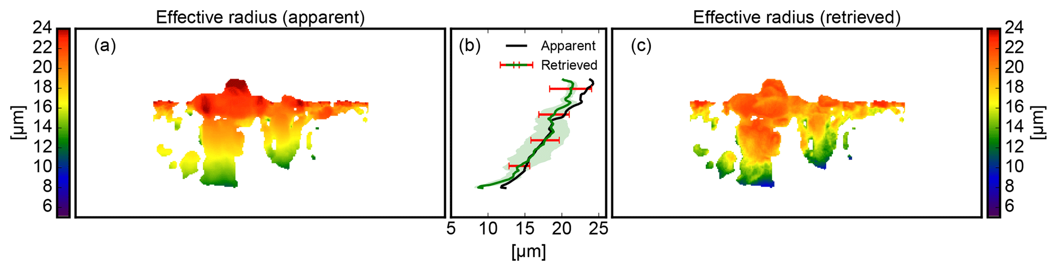
Figure 21Retrieval comparison between the apparent effective radius (a) and the retrieved mean effective radius (c) for a cloud scene that was not included in the forward ensemble. (a) Apparent effective radius 〈reff〉app for the airborne perspective, (b) mean and standard deviation of the apparent (black) and retrieved (green) vertical effective radius profile with the mean statistical retrieval uncertainty (red error bars). (c) Retrieved mean effective radius for the airborne perspective.
Like in Fig. 19b, σ(reff) increases with reff from to . Within σ(reff), the retrieval reproduces the mean effective radius profile for all three cases quite well. For some specific cloud regions, however, there are also large differences of up to ±3 µm. This is especially true at cloud edges and close to shadows.
Altogether, the statistical relationship between reflected radiance and cloud droplet size seems stable enough to be used for highly complex cloud sides. Moreover, these first results indicate that the retrieval seems to be resilient to the unrealistic, flipped cloud profiles included in its lookup table. Although the retrieval showed minor problems in retrieving the flipped profile, no substantial bias towards a specific effective radius profile could be detected. Mean values for all heights agree within the natural variability in the LES data; the retrieval error estimate σ(reff) seems to overestimate the uncertainty. Since these results were only obtained for a single cloud side scene, the following section will investigate these findings for a representative number of scenes.
6.1.1 Statistic stability for included scenes
In the first step, the retrieval will be tested for perspectives which are already included in the lookup table. This is done to test the retrieval for biases and to obtain a robust measure of correlation between the retrieval and the cloud side scenes it is composed of. By comparing this correlation with the correlation for cloud side scenes that are not included in the lookup table, this analysis will also be used to detect a potential over-fitting. There is the risk that the lookup table only reflects 3-D effects that are specific for the included cloud side scenes.
In total, nine cloud side perspectives were randomly chosen from the polluted as well as the clean data set. For each perspective, the normal, the flipped as well as the fixed effective radius profile were tested. This amounts to test cases. For this statistical comparison, only reliable results with a retrieval error estimate σ(reff) of less than 2.5 µm were included.
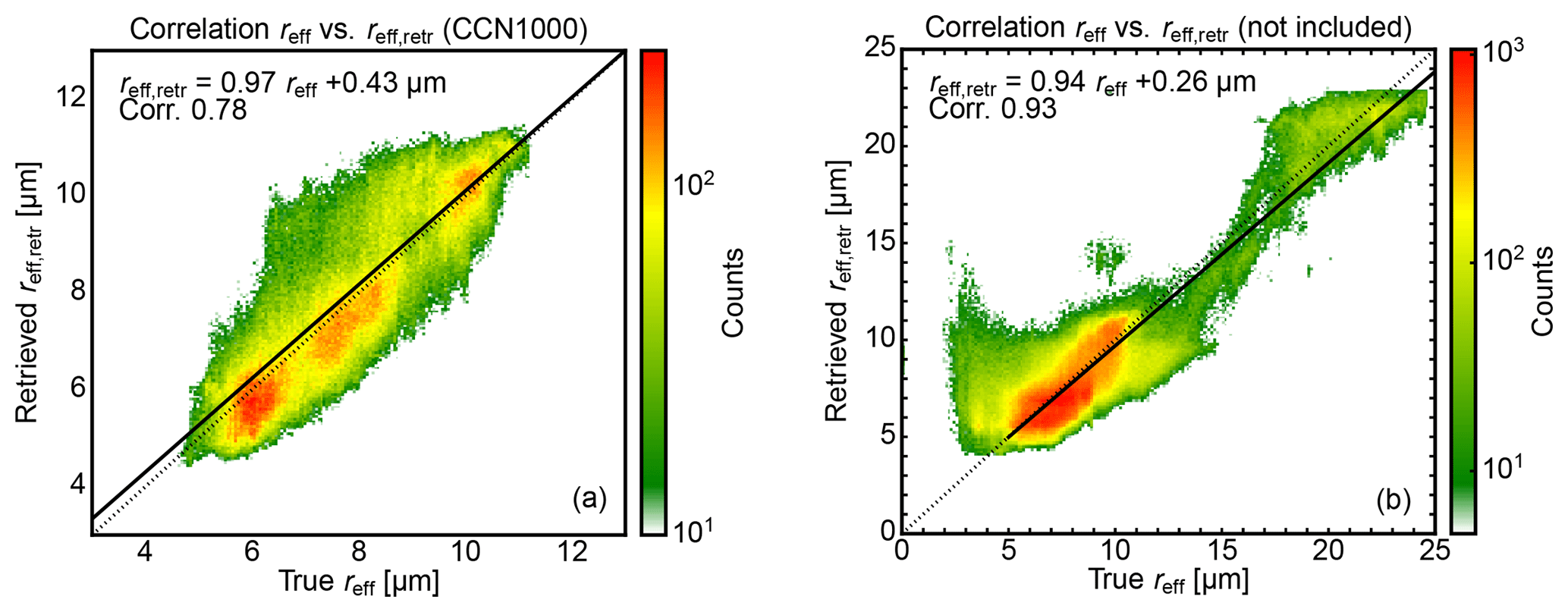
Figure 22Two-dimensional histograms and linear regressions to determine the correlation between the apparent effective radius reff and the retrieved effective radius reff,retr for (a) the included polluted cases () with normal and flipped effective radius profile, and (b) for the not included cases with normal and flipped effective radius profile.
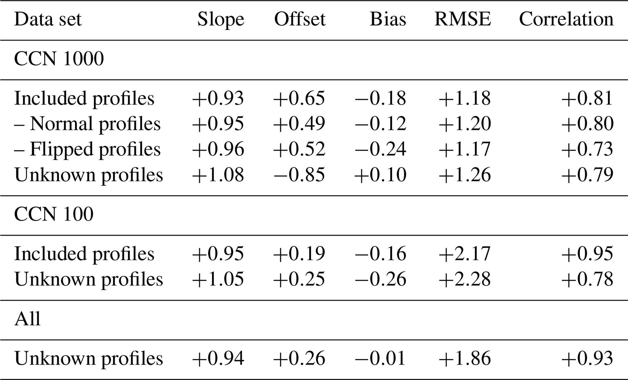
Figure 22a shows the correlation for the normal and the flipped polluted profiles which include around 358 000 pixels. The linear regression with a slope of 0.97 and an offset of 0.43 µm shows no significant retrieval bias for these cases. The correlation between the apparent and the retrieved values is 0.78. A deeper insight can be gained through Table 2, where all comparisons are summarized separately for normal and flipped profiles. The higher correlation coefficient (0.80 vs. 0.73) seems to indicate a slightly better ability to detect the cases with a normal effective radius profile. Nevertheless, comparable linear regressions show no substantial bias towards the normal or the flipped cases. This confirms the observation made in the case study shown in Fig. 20.
For the fixed effective radius profiles, the histogram in Fig. 23 shows the deviation of the statistical retrieval with two distinct modes. With most likely values between 0 µm and −1 µm, the retrieval underestimates the effective radius slightly. A second mode is found where the retrieval overestimates reff with values between 1 and 2 µm. In combination, there is only a slight overestimation of 0.10 µm with a larger standard deviation of 1.17 µm. A further investigation showed that the overestimation peak is connected with and found around undetected cloud shadows.
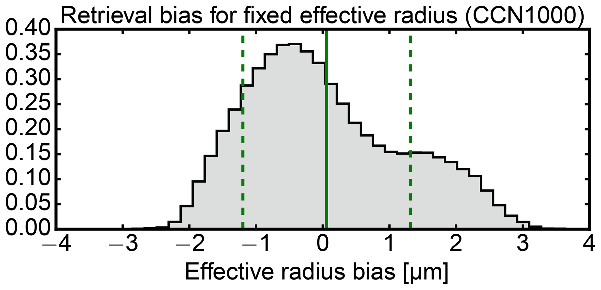
Figure 23Retrieval deviations (retrieved reff,retr – apparent reff) for the nine cloud sides with fixed effective radius profiles which are not included in the ensemble. The solid green line shows the average bias in retrieved effective radius reff,retr, the dashed green lines show the RMSE for reff,retr.
6.1.2 Statistic stability for unknown scenes
To check the retrieval for potential over-fitting, the retrieval was applied to unknown cloud side scenes. Nine new cloud side perspectives were selected from the polluted and the clean LES runs. While the forward ensemble contains viewing azimuths of 45, 135, 225, and 315∘, these new cloud side perspectives were chosen for new viewing azimuths of 0, 90, 180, and 270∘ and only normal effective radius profiles were used this time.
Figure 21 shows one of these new cloud side scenes with a normal effective radius profile. In contrast to Fig. 20, this clean () scene features a much larger range of cloud droplet sizes. For this scene with overall larger reff, the retrieval underestimates reff by ±2.5 µm at the upper cloud side part. Nevertheless, the statistical retrieval detects the mean effective radius profiles well within σ(reff). Like in Fig. 20a, σ(reff) increases with reff from to .
The comparison for all not included cloud sides is shown in Fig. 22b. The correlation for the not included cases is 0.93, where around 339 000 pixels are compared in total.
With nearly the same correlation coefficient, the retrieval performance remains the same when faced with unknown cloud side scenes. It can therefore be concluded that the retrieval is not only trained for the included cloud side scenes. Rather, it represents the statistical relationship between reflected radiance and cloud droplet size for this cloud ensemble.
Table 2Results of retrieval performance tests when faced with normal, flipped, and not included effective radius profiles, grouped for CCN=1000, CCN=100, and for all not included cases. Linear regression, bias, root-mean-square error (RMSE), and correlation are calculated between apparent and retrieved effective radius.
The presented work advanced a framework for the remote sensing of cloud droplet effective radius profiles from cloud sides, which was introduced by Marshak et al. (2006a), Zinner et al. (2008), and Martins et al. (2011). Up until now, their approach could not be directly applied to realistic cloud side measurements (e.g., specMACS on HALO) since their studies lack the varying geometries of an airborne perspective. Furthermore, the effective radius was only parameterized and not directly calculated by a microphysical model. Moreover, Zinner et al. (2008) used the line of sight method to associate the forward modeled radiance with reff found at the first cloudy grid box. To advance the technique to realistic airborne measurements, this study addressed the following scientific objectives to overcome these limitations.
-
First, by extending the existing approach to realistic airborne perspectives and developing methods to test the sensitivity of reflected radiances from cloud sides to cloud droplet radius, where the observer position is located within the cloud field. To this end, methods were developed to identify suitable observation positions within a model cloud field and to calculate an apparent effective radius for each forward modeled sensor pixel.
-
In the course of this process, 3-D radiative effects caused by the unknown cloud surface orientation were investigated. A technique was proposed to mitigate their impact on cloud droplet size retrievals by putting pixels in context with their surroundings.
-
Finally, an effective radius retrieval for the cloud side perspective was developed and tested for cloud scenes, which were used during the retrieval development, as well as for unknown scenes.
The scope of this work was limited to the liquid part of convective water clouds, e.g., cumulus mediocris, cumulus congestus, and trade-wind cumulus, which exhibit well-developed cloud sides. In principle, the proposed technique could also be extended to ice clouds.
In the first step, this work introduced a statistical framework for the proposed remote sensing of cloud sides following Marshak et al. (2006a). A statistical relationship between reflected sunlight in a near-visible and near-infrared wavelength and droplet size was found following the classical approach by Nakajima and King (1990). By simulating the three-dimensional radiative transfer for high-resolution LES model clouds using the 3-D Monte Carlo radiative transfer model MYSTIC, probability distributions for this relationship were sampled. These distributions describe the probability to find a specific droplet size after a specific solar reflectance pair of values has been measured. In contrast to many other effective radius retrievals, this work thereby provides essential information about the retrieval uncertainties which are intrinsically linked with the reflectance ambiguities caused by three-dimensional radiative effects. Furthermore, this work developed a technique (Sect. 4.3) to reduce 3-D radiance ambiguities when no information about the cloud surface orientation is available. More precisely, additional information from surrounding pixels was used to classify the environment of the considered pixel. Subsequently, this technique and the forward simulated probability distributions were incorporated into a statistical retrieval of the effective radius from cloud sides. Defined by the used LES model fields and the chosen geometries of the forward simulations, this retrieval is designed for
-
cloud side measurements of the liquid part of convective water clouds, e.g., cumulus mediocris, cumulus congestus, and trade-wind cumulus, which exhibit well-developed cloud sides;
-
cloud tops between 1.5 and 2 km, an optical thickness between 15 and 150 and effective radii between 4 and 24 µm;
-
spatially highly resolved (10 × 10 m) images of the spectral radiance at λ=870 and λ=2100 nm;
-
a variable and unknown CCN background concentration between 100 to 1000 cm−3;
-
variable sun zenith angles ϑ0 from 7 to 67∘ for tropical as well as mid-latitude application;
-
an airborne perspective at a low-level altitude with a field of view of (azimuthal) and (horizontal) centered 5∘ below the horizon.
The numerical analysis of the statistical retrieval showed a RMSE between retrieved and apparent reff of around 1 to 1.5 µm. For the intended airborne measurement perspective (see Part 2 of this work), the statistical retrieval reliably detects the present effective radius profile, while sanity checks showed no prior bias of the retrieval towards specific cloud droplet size profiles. This is an essential prerequisite for all consecutive interpretations of the retrieval results. Furthermore, the retrieval performance remained the same when faced with unknown cloud side scenes not included in the ensemble used for the retrieval. It can therefore be concluded that the retrieval is not over-fitted and that it represents the statistical relationship between reflected radiance and cloud droplet size for this cloud side perspective.
Moreover, this work dissected the impact of an unknown cloud surface orientation on bi-spectral effective radius retrievals using an optically thick water cloud sphere (τc=500). Just with every other 3-D cloud side scene, some local viewing angles onto cloud surfaces are steeper while some viewing perspectives onto cloud surfaces are more oblique than the local illumination angle. As a consequence, the correlation between reflected solar radiance pairs and droplet sizes becomes ambiguous.
This study did not address the open question of whether strong rain can influence the retrieval performance and how. Several studies (Nakajima et al., 2009; Zinner et al., 2010; Zhang et al., 2012) found only a small impact of drizzle on bi-spectral methods of about 0.5 to 2 µm. Although beyond the scope of this work, subsequent studies should address the influence of rain on bi-spectral retrievals for stronger precipitation rates, as suggested by the more recent study of Zhang (2013).
The next important step is the application of the proposed retrieval technique to real measurements. In combination with simultaneous in situ measurements, airborne cloud side observations have been acquired with the hyperspectral cloud and sky imager specMACS. In a follow-up paper (Part 2), the proposed retrieval will be validated with this independent in situ data.
A further important point is the development of a distance mapping for the retrieval. The height and location assignment of retrieval results is not just of uttermost importance for the comparison with in situ measurements and models, but also essential to estimate the cloud distance for a potential aerosol correction. Here, first promising results could be achieved by exploiting the oxygen A-band absorption at λ=762 nm presented in Zinner et al. (2019). In conclusion, the present work developed a working effective radius retrieval for measurements of cloud sides applicable to real measurements and thus paved the way for further research on this topic.
All data sets used in this publication are provided upon request.
TZ, BM, and FE conceived and planned the retrieval concept. FE developed the presented methods and carried out the model simulations and their analysis. FE, TZ, TK, and BM contributed to the interpretation of the results. FE took the lead in writing the manuscript. All authors provided feedback on the manuscript.
The authors declare that they have no conflict of interest.
We would like to thank Graham Feingold for providing the RICO cloud model
fields. Thanks and acknowledgment also go to Silke Groß and the DLR
Institute of Atmospheric Physics, who supported the completion of this
paper. Florian Ewald was partly funded by the German Research Foundation
(DFG) under grant no. MA 2548/9-1. Tobias Kölling was supported by the
German Research Foundation (DFG) under grant no. Zi 1132/3-1. We thank two
anonymous reviewers for their comments and suggestions.
The article processing charges for this open-access
publication were covered by a Research
Centre of the Helmholtz Association.
Edited by: Alexander Kokhanovsky
Reviewed by: two anonymous referees
Alexandrov, M. D., Cairns, B., Emde, C., Ackerman, A. S., and van Diedenhoven, B.: Accuracy assessments of cloud droplet size retrievals from polarized reflectance measurements by the research scanning polarimeter, Remote Sens. Environ., 125, 92–111, https://doi.org/10.1016/j.rse.2012.07.012, 2012. a
Anderson, G., Clough, S., Kneizys, F., Chetwynd, J., and Shettle, E.: AFGL Atmospheric Constituent Profiles (0–120 km), Tech. Rep. AFGL-TR-86-0110, 1986. a
Andreae, M. O., Afchine, A., Albrecht, R., Holanda, B. A., Artaxo, P., Barbosa, H. M. J., Borrmann, S., Cecchini, M. A., Costa, A., Dollner, M., Fütterer, D., Järvinen, E., Jurkat, T., Klimach, T., Konemann, T., Knote, C., Krämer, M., Krisna, T., Machado, L. A. T., Mertes, S., Minikin, A., Pöhlker, C., Pöhlker, M. L., Pöschl, U., Rosenfeld, D., Sauer, D., Schlager, H., Schnaiter, M., Schneider, J., Schulz, C., Spanu, A., Sperling, V. B., Voigt, C., Walser, A., Wang, J., Weinzierl, B., Wendisch, M., and Ziereis, H.: Aerosol characteristics and particle production in the upper troposphere over the Amazon Basin, Atmos. Chem. Phys., 18, 921–961, https://doi.org/10.5194/acp-18-921-2018, 2018. a
Arabas, S., Pawlowska, H., and Grabowski, W. W.: Effective radius and droplet spectral width from in-situ aircraft observations in trade-wind cumuli during RICO, Geophys. Res. Lett., 36, L11803, https://doi.org/10.1029/2009GL038257, 2009. a
Buras, R. and Mayer, B.: Efficient unbiased variance reduction techniques for Monte Carlo simulations of radiative transfer in cloudy atmospheres: the solution, J. Quant. Spectrosc. Ra., 112, 434–447, 2011. a, b
Cahalan, R. F., Ridgway, W., Wiscombe, W., and Bell, T.: The albedo of fractal stratocumulus clouds, J. Atmos. Sci., 51, 2434–2455, 1994. a
Ehrlich, A., Bierwirth, E., Wendisch, M., Gayet, J.-F., Mioche, G., Lampert, A., and Heintzenberg, J.: Cloud phase identification of Arctic boundary-layer clouds from airborne spectral reflection measurements: test of three approaches, Atmos. Chem. Phys., 8, 7493–7505, https://doi.org/10.5194/acp-8-7493-2008, 2008. a
Eichler, H., Ehrlich, A., Wendisch, M., Mioche, G., Gayet, J.-F., Wirth, M., Emde, C., and Minikin, A.: Influence of ice crystal shape on retrieval of cirrus optical thickness and effective radius: A case study, J. Geophys. Res.-Atmos., 114, D19203, https://doi.org/10.1029/2009JD012215, 2009. a
Emde, C., Buras-Schnell, R., Kylling, A., Mayer, B., Gasteiger, J., Hamann, U., Kylling, J., Richter, B., Pause, C., Dowling, T., and Bugliaro, L.: The libRadtran software package for radiative transfer calculations (version 2.0.1), Geosci. Model Dev., 9, 1647–1672, https://doi.org/10.5194/gmd-9-1647-2016, 2016. a
Ewald, F., Zinner, T., and Mayer, B.: Remote sensing of particle size profiles from cloud sides: Observables and retrievals in a 3-D environment, in: AIP Conference Proceedings, 1531, 83–86, AIP Publishing, https://doi.org/10.1063/1.4804713, 2013. a, b, c
Ewald, F., Kölling, T., Baumgartner, A., Zinner, T., and Mayer, B.: Design and characterization of specMACS, a multipurpose hyperspectral cloud and sky imager, Atmos. Meas. Tech., 9, 2015–2042, https://doi.org/10.5194/amt-9-2015-2016, 2016. a
Feingold, G., Kreidenweis, S. M., Stevens, B., and Cotton, W. R.: Numerical simulations of stratocumulus processing of cloud condensation nuclei through collision-coalescence, J. Geophys. Res.-Atmos., 101, 21391–21402, https://doi.org/10.1029/96JD01552, 1996. a
Gasteiger, J., Emde, C., Mayer, B., Buras, R., Buehler, S. A., and Lemke, O.: Representative wavelengths absorption parameterization applied to satellite channels and spectral bands, J. Quant. Spectrosc. Ra., 148, 99–115, https://doi.org/10.1016/j.jqsrt.2014.06.024, 2014. a, b
Han, Q., Rossow, W., and Lacis, A.: Near-global survey of effective droplet radii in liquid water clouds using ISCCP data, J. Climate, 7, 465–497, 1994. a
Hess, M., Koepke, P., and Schult, I.: Optical Properties of Aerosols and Clouds: The Software Package OPAC, B. Am. Meteor. Soc., 79, 831–844, https://doi.org/10.1175/1520-0477(1998)079<0831:OPOAAC>2.0.CO;2, 1998. a
Jäkel, E., Walter, J., and Wendisch, M.: Thermodynamic phase retrieval of convective clouds: impact of sensor viewing geometry and vertical distribution of cloud properties, Atmos. Meas. Tech., 6, 539–547, https://doi.org/10.5194/amt-6-539-2013, 2013. a
Jiang, G. M. and Li, Z. L.: Cross-calibration of MSG1-SEVIRI infrared channels with Terra-MODIS channels, Int. J. Remote Sens., 30, 753–769, https://doi.org/10.1080/01431160802392638, 2009. a, b, c, d
King, M.: Determination of the scaled optical thickness of clouds from reflected solar radiation measurements, J. Atmos. Sci., 44, 1734–1751, 1987. a
Krautstrunk, M. and Giez, A.: The Transition From FALCON to HALO Era Airborne Atmospheric Research, in: Atmospheric Physics, edited by: Schumann, U., Research Topics in Aerospace, 609–624, Springer Berlin Heidelberg, 2012. a
Kurucz, R. L.: Synthetic Infrared Spectra, in: Infrared Solar Physics, edited by Rabin, D. M., Jefferies, J. T., and Lindsey, C., 154, 523, IAU Symposium, 1994. a
Marshak, A., Martins, J. V., Zubko, V., and Kaufman, Y. J.: What does reflection from cloud sides tell us about vertical distribution of cloud droplet sizes?, Atmos. Chem. Phys., 6, 5295–5305, https://doi.org/10.5194/acp-6-5295-2006, 2006a. a, b, c, d, e, f
Marshak, A., Platnick, S., Varnai, T., Wen, G., and Cahalan, R. F.: Impact of three-dimensional radiative effects on satellite retrievals of cloud droplet sizes, Journal of Geophysical Research, 111, D09207, https://doi.org/10.1029/2005JD006686, 2006b. a
Martin, G. M., Johnson, D. W., and Spice, A.: The Measurement and Parameterization of Effective Radius of Droplets in Warm Stratocumulus Clouds, J. Atmos. Sci., 51, 1823–1842, https://doi.org/10.1175/1520-0469(1994)051<1823:TMAPOE>2.0.CO;2, 1994. a
Martins, J. V., Marshak, A., Remer, L. A., Rosenfeld, D., Kaufman, Y. J., Fernandez-Borda, R., Koren, I., Correia, A. L., Zubko, V., and Artaxo, P.: Remote sensing the vertical profile of cloud droplet effective radius, thermodynamic phase, and temperature, Atmos. Chem. Phys., 11, 9485–9501, https://doi.org/10.5194/acp-11-9485-2011, 2011. a, b, c
Mayer, B. and Kylling, A.: Technical note: The libRadtran software package for radiative transfer calculations – description and examples of use, Atmos. Chem. Phys., 5, 1855–1877, https://doi.org/10.5194/acp-5-1855-2005, 2005. a
Mayer, B.: Radiative transfer in the cloudy atmosphere, Eur. Physical J. Conf., 1, 75–99, 2009. a, b
McBride, P. J., Schmidt, K. S., Pilewskie, P., Kittelman, A. S., and Wolfe, D. E.: A spectral method for retrieving cloud optical thickness and effective radius from surface-based transmittance measurements, Atmos. Chem. Phys., 11, 7235–7252, https://doi.org/10.5194/acp-11-7235-2011, 2011. a
Miller, D. J., Zhang, Z., Ackerman, A. S., Platnick, S., and Baum, B. A.: The impact of cloud vertical profile on liquid water path retrieval based on the bispectral method: A theoretical study based on large-eddy simulations of shallow marine boundary layer clouds, J. Geophys. Res., 121, 4122–4141, https://doi.org/10.1002/2015JD024322, 2016. a
Miller, D. J., Zhang, Z., Platnick, S., Ackerman, A. S., Werner, F., Cornet, C., and Knobelspiesse, K.: Comparisons of bispectral and polarimetric retrievals of marine boundary layer cloud microphysics: case studies using a LES-satellite retrieval simulator, Atmos. Meas. Tech., 11, 3689–3715, https://doi.org/10.5194/amt-11-3689-2018, 2018. a
Mosegaard, K. and Tarantola, A.: Monte Carlo sampling of solutions to inverse problems, J. Geophys. Res.-Sol. Ea., 100, 12431–12447, https://doi.org/10.1029/94JB03097, 1995. a, b
Nakajima, T. Y. and King, M. D.: Determination of the optical thickness and effective particle radius of clouds from reflected solar radiation measurements, Part I: Theory, J. Atmos. Sci, 47, 1878–1893, 1990. a, b, c, d, e
Nakajima, T. Y., Suzuki, K., and Stephens, G. L.: Droplet Growth in Warm Water Clouds Observed by the A-Train, Part I: Sensitivity Analysis of the MODIS-Derived Cloud Droplet Sizes, J. Atmos. Sci., 67, 1884–1896, 2009. a
Okamura, R., Iwabuchi, H., and Schmidt, K. S.: Feasibility study of multi-pixel retrieval of optical thickness and droplet effective radius of inhomogeneous clouds using deep learning, Atmos. Meas. Tech., 10, 4747–4759, https://doi.org/10.5194/amt-10-4747-2017, 2017. a
Pilewskie, P., Pommier, J., Bergstrom, R., Gore, W., Rabbette, M., Schmid, B., Hobbs, P. V., and Tsay, S. C.: Solar spectral radiative forcing during the Southern African regional science initiative, J. Geophys. Res., 108, 8486, https://doi.org/10.1029/2002JD002411, 2003. a
Plass, G. N. and Kattawar, G. W.: Influence of Single Scattering Albedo on Reflected and Transmitted Light from Clouds, Appl. Opt., 7, 361–367, https://doi.org/10.1364/AO.7.000361, 1968. a
Platnick, S.: Vertical photon transport in cloud remote sensing problems, Jo. Geophys. Res., 105, 22919–22935, 2000. a, b, c, d
Platnick, S., Li, J., King, M. D., Gerber, H., and Hobbs, P.: A solar reflectance method for retrieving the optical thickness and droplet size of liquid water clouds over snow and ice surfaces, J. Geophys. Res., 106, 15, 2001. a
Rauber, R. M., Ochs, H. T., Di Girolamo, L., Göke, S., Snodgrass, E., Stevens, B., Knight, C., Jensen, J. B., Lenschow, D. H., Rilling, R. A., Rogers, D. C., Stith, J. L., Albrecht, B. A., Zuidema, P., Blyth, A. M., Fairall, C. W., Brewer, W. A., Tucker, S., Lasher-Trapp, S. G., Mayol-Bracero, O. L., Vali, G., Geerts, B., Anderson, J. R., Baker, B. A., Lawson, R. P., Bandy, A. R., Thornton, D. C., Burnet, E., Brenguier, J.-L., Gomes, L., Brown, P. R. A., Chuang, P., Cotton, W. R., Gerber, H., Heikes, B. G., Hudson, J. G., Kollias, P., Krueger, S. K., Nuijens, L., O'Sullivan, D. W., Siebesma, A. P., and Twohy, C. H.: Rain in Shallow Cumulus Over the Ocean: The RICO Campaign, B. Am. Meteor. Soc., 88, 1912–1928, https://doi.org/10.1175/BAMS-88-12-1912, 2007. a, b
Roebeling, R. A., Feijt, A. J., and Stammes, P.: Cloud property retrievals for climate monitoring: Implications of differences between Spinning Enhanced Visible and Infrared Imager (SEVIRI) on METEOSAT-8 and Advanced Very High Resolution Radiometer (AVHRR) on NOAA-17, J. Geophys. Res., 111, D20210, https://doi.org/10.1029/2005JD006990, 2006. a
Rosenfeld, D., Williams, E., Andreae, M. O., Freud, E., Pöschl, U., and Rennó, N. O.: The scientific basis for a satellite mission to retrieve CCN concentrations and their impacts on convective clouds, Atmos. Meas. Tech., 5, 2039–2055, https://doi.org/10.5194/amt-5-2039-2012, 2012. a
Rothman, L. S., Jacquemart, D., Barbe, A., Benner, D. C., Birk, M., Brown, L. R., Carleer, M. R., Chackerian Jr., C., Chance, K., Coudert, L. H., Dana, V., Devi, V. M., Flaud, J., Gamache, R. R., Goldman, A., Hartmann, J., Jucks, K. W., Maki, A. G., Mandin, J., Massie, S. T., Orphal, J., Perrin, A., Rinsland, C. P., Smith, M. A. H., Tennyson, J., Tolchenov, R. N., Toth, R. A., Vander Auwera, J., Varanasi, P., and Wagner, G.: The HITRAN 2004 molecular spectroscopic database, J. Quant. Spectrosc. Ra., 96, 139–204, 2005. a
Schmidt, K., Pilewskie, P., Platnick, S., Wind, G., Yang, P., and Wendisch, M.: Comparing irradiance fields derived from Moderate Resolution Imaging Spectroradiometer airborne simulator cirrus cloud retrievals with solar spectral flux radiometer measurements, J. Geophys. Res, 112, D24206, https://doi.org/10.1029/2007JD008711, 2007. a
Scott, D. W., Tapia, R. A., and Thompson, J. R.: Kernel density estimation revisited, Nonlinear Anal.-Theor., 1, 339–372, https://doi.org/10.1016/S0362-546X(97)90003-1, 1977. a
Stamnes, K., Tsay, S.-C., Wiscombe, W., and Jayaweera, K.: A numerically stable algorithm for discrete-ordinate-method radiative transfer in multiple scattering and emitting layered media, Appl. Opt., 27, 2502–2509, 1988. a
Tzivion, S., Feingold, G., and Levin, Z.: An Efficient Numerical Solution to the Stochastic Collection Equation, J. Atmos. Sci., 44, 3139–3149, https://doi.org/10.1175/1520-0469(1987)044<3139:AENSTT>2.0.CO;2, 1987. a
Tzivion, S., Feingold, G., and Levin, Z.: The Evolution of Raindrop Spectra, Part II: Collisional Collection/Breakup and Evaporation in a Rainshaft, J. Atmos. Sci., 46, 3312–3328, https://doi.org/10.1175/1520-0469(1989)046<3312:TEORSP>2.0.CO;2, 1989. a
Vant-Hull, B., Marshak, A., Remer, L., and Li, Z.: The effects of scattering angle and cumulus cloud geometry on satellite retrievals of cloud droplet effective radius, IEEE T. Geosci. Remote, 45, 1039–1045, 2007. a, b
Varnai, T. and Marshak, A.: Observations of the three-dimensional radiative effects that influence MODIS cloud optical thickness retrievals, J. Atmos. Sci., 59, 1607–1618, 2002. a
Varnai, T. and Marshak, A.: A method for analyzing how various parts of clouds influence each other's brightness, J. Geophys. Res., 108, 4706, https://doi.org/10.1029/2003JD003561, 2003. a
Varnai, T. and Marshak, A.: View angle dependence of cloud optical thicknesses retrieved by Moderate Resolution Imaging Spectroradiometer (MODIS), J. Geophys. Res., 112, D06203, https://doi.org/10.1029/2005JD006912, 2007. a
Wendisch, M., Müller, D., Schell, D., and Heintzenberg, J.: An airborne spectral albedometer with active horizontal stabilization, J. Atmos. Ocean. Tech., 18, 1856–1866, 2001. a
Wendisch, M. and Mayer, B.: Vertical distribution of spectral solar irradiance in the cloudless sky – A case study, Geophys. Res. Lett., 30, 1183, https://doi.org/10.1029/2002GL016529, 2003. a
Wendisch, M., Pöschl, U., Andreae, M. O., Machado, L. A., Albrecht, R., Schlager, H., Rosenfeld, D., Martin, S. T., Abdelmonem, A., Afchine, A., Araùjo, A. C., Artaxo, P., Aufmhoff, H., Barbosa, H. M., Borrmann, S., Braga, R., Buchholz, B., Cecchini, M. A., Costa, A., Curtius, J., Dollner, M., Dorf, M., Dreiling, V., Ebert, V., Ehrlich, A., Ewald, F., Fisch, G., Fix, A., Frank, F., Fütterer, D., Heckl, C., Heidelberg, F., Hüneke, T., Jäkel, E., Järvinen, E., Jurkat, T., Kanter, S., Kästner, U., Kenntner, M., Kesselmeier, J., Klimach, T., Knecht, M., Kohl, R., Kölling, T., Krämer, M., Krüger, M., Krisna, T. C., Lavric, J. V., Longo, K., Mahnke, C., Manzi, A. O., Mayer, B., Mertes, S., Minikin, A., Molleker, S., Münch, S., Nillius, B., Pfeilsticker, K., Pöhlker, C., Roiger, A., Rose, D., Rosenow, D., Sauer, D., Schnaiter, M., Schneider, J., Schulz, C., de Souza, R. A., Spanu, A., Stock, P., Vila, D., Voigt, C., Walser, A., Walter, D., Weigel, R., Weinzierl, B., Werner, F., Yamasoe, M. A., Ziereis, H., Zinner, T., and Zöger, M.: ACRIDICON-CHUVA Campaign: Studying Tropical Deep Convective Clouds and Precipitation over Amazonia Using the New German Research Aircraft HALO, B. Am. Meteor. Soc., 97, 1885–1908, https://doi.org/10.1175/BAMS-D-14-00255.1, 2016. a
Wiscombe, W.: Improved Mie scattering algorithms, Appl. Opt., 19, 1505–1509, 1980. a
Yang, P., Wei, H., Baum, B., Huang, H., Heymsfield, A., Hu, Y., Gao, B., and Turner, D.: The spectral signature of mixed-phase clouds composed of non-spherical ice crystals and spherical liquid droplets in the terrestrial window region, J. Quant. Spectrosc. Ra., 79, 1171–1188, 2003. a, b
Yuter, S. E. and Houze, R. A.: Three-Dimensional Kinematic and Microphysical Evolution of Florida Cumulonimbus, Part II: Frequency Distributions of Vertical Velocity, Reflectivity, and Differential Reflectivity, Mon. Weather Rev., 123, 1941–1963, https://doi.org/10.1175/1520-0493(1995)123<1941:TDKAME>2.0.CO;2, 1995. a
Zhang, Z., Ackerman, A. S., Feingold, G., Platnick, S., Pincus, R., and Xue, H.: Effects of cloud horizontal inhomogeneity and drizzle on remote sensing of cloud droplet effective radius: Case studies based on large-eddy simulations, J. Geophys. Res.-Atmos., 117, D19208, https://doi.org/10.1029/2012JD017655, 2012. a
Zhang, Z.: On the sensitivity of cloud effective radius retrieval based on spectral method to bi-modal droplet size distribution: A semi-analytical model, J. Quant. Spectrosc. Ra., 129, 79–88, 2013. a
Zhang, Z., Dong, X., Xi, B., Song, H., Ma, P. L., Ghan, S. J., Platnick, S., and Minnis, P.: Intercomparisons of marine boundary layer cloud properties from the ARM CAP-MBL campaign and two MODIS cloud products, J. Geophys. Res., 122, 2351–2365, https://doi.org/10.1002/2016JD025763, 2017. a
Zinner, T. and Mayer, B.: Remote sensing of stratocumulus clouds: Uncertainties and biases due to inhomogeneity, J. Geophys. Res., 111, D14209, https://doi.org/10.1029/2005JD006955, 2006. a, b
Zinner, T., Marshak, A., Lang, S., Martins, J. V., and Mayer, B.: Remote sensing of cloud sides of deep convection: towards a three-dimensional retrieval of cloud particle size profiles, Atmos. Chem. Phys., 8, 4741–4757, https://doi.org/10.5194/acp-8-4741-2008, 2008. a, b, c, d, e, f, g, h, i, j
Zinner, T., Wind, G., Platnick, S., and Ackerman, A. S.: Testing remote sensing on artificial observations: impact of drizzle and 3-D cloud structure on effective radius retrievals, Atmos. Chem. Phys., 10, 9535–9549, https://doi.org/10.5194/acp-10-9535-2010, 2010. a
Zinner, T., Schwarz, U., Kölling, T., Ewald, F., Jäkel, E., Mayer, B., and Wendisch, M.: Cloud geometry from oxygen-A-band observations through an aircraft side window, Atmos. Meas. Tech., 12, 1167–1181, https://doi.org/10.5194/amt-12-1167-2019, 2019. a