Flow-induced errors in airborne in situ measurements of aerosols and clouds

Aerosols and clouds affect atmospheric radiative processes and climate in many complex ways and still pose the largest uncertainty in current estimates of the Earth's changing energy budget.

Airborne in situ sensors such as the Cloud, Aerosol, and Precipitation Spectrometer (CAPS) or other optical spectrometers and optical array probes provide detailed information about the horizontal and vertical distribution of aerosol and cloud properties. However, flow distortions occurring at the location where these instruments are mounted on the outside of an aircraft may directly produce artifacts in detected particle number concentration and also cause droplet deformation and/or breakup during the measurement process.

Several studies have investigated flow-induced errors assuming that air is incompressible. However, for fast-flying aircraft, the impact of air compressibility is no longer negligible. In this study, we combine airborne data with numerical simulations to investigate the flow around wing-mounted instruments and the induced errors for different realistic flight conditions. A correction scheme for deriving particle number concentrations from in situ aerosol and cloud probes is proposed, and a new formula is provided for deriving the droplet volume from images taken by optical array probes. Shape distortions of liquid droplets can either be caused by errors in the speed with which the images are recorded or by aerodynamic forces acting at the droplet surface caused by changes of the airflow when it approaches the instrument. These forces can lead to the dynamic breakup of droplets causing artifacts in particle number concentration and size. An estimation of the critical breakup diameter as a function of flight conditions is provided.

Experimental data show that the flow speed at the instrument location is smaller than the ambient flow speed. Our simulations confirm the observed difference and reveal a size-dependent impact on particle speed and concentration. This leads, on average, to a 25 % overestimation of the number concentration of particles with diameters larger than 10 µm diameter and causes distorted images of droplets and ice crystals if the flow values recorded at the instrument are used. With the proposed corrections, errors of particle number concentration and droplet volume, as well as image distortions, are significantly reduced by up to 1 order of magnitude.

Although the presented correction scheme is derived for the DLR Falcon research aircraft (Saharan Aerosol Long-range Transport and Aerosol-Cloud-Interaction Experiment (SALTRACE) campaign) and validated for the DLR Falcon (Absorbing aerosol layers in a changing climate: aging, lifetime and dynamics mission conducted in 2017 (A-LIFE) campaign) and the NASA DC-8 (Atmospheric Tomography Mission (ATom) campaigns), the general conclusions hold for any fast-flying research aircraft.

1 Introduction

Aerosol–cloud–radiation interactions are one of the largest uncertainties in current climate predictions (Stocker et al., 2014). The size distribution of cloud and aerosol particles is a crucial parameter for aerosol–radiation and aerosol–cloud interaction (Albrecht, 1989; Rosenfeld and Lensky, 1998; Pruppacher and Klett, 2010). For example, an increase of the fraction of coarse particles can modify the direct radiative forcing of desert dust from cooling to warming (Kok et al., 2017) and also increase the reservoir of ice-nucleating particles (e.g., DeMott et al., 2010).

Airborne in situ measurements are fundamental to extend our knowledge of cloud and aerosol distributions, especially in the coarse mode. Instruments typically used by the aerosol and cloud community, for measuring coarse particles, are open-path or passive-inlet¹ optical particle counters (OPCs) and optical array probes (OAPs). OPCs and OAPs measure particle flux as they record, within a time interval, the number of particles passing through a specific region named sampling area. The flux is later converted into a concentration using the airflow speed. Therefore, errors in the flow speed are directly affecting the calculated particle and cloud hydrometeor concentrations. For example, a too-low flow speed leads to a higher calculated particle concentration. Since the aircraft itself can influence the surrounding air and the flow measurements (Kalogiros and Wang, 2002), airborne measurements are challenging. Flow distortion caused by the fuselage and wings not only impacts the flow velocity but also modifies air temperature, pressure, and density as compared to free stream conditions, thereby further affecting the aerosol and cloud measurements. For example, a higher air density leads to a higher number concentration of aerosol particles if the particles are sufficiently small to be able to follow the airflow. Furthermore, large droplets may be deformed or may even break up during high-speed sampling due to aerodynamic forces acting on the droplet surface, as studied by Szakall et al. (2009); Vargas and Feo (2010). Whereas droplet deformation does not change the detected number concentrations, breakup results in enhanced droplet number concentrations (Weber et al., 1998). These shattering artifacts may originate not only from aerodynamic forces but also from impaction breakup of cloud droplets and ice particles in and around the aerosol inlet (Korolev and Isaac, 2005; Craig et al., 2013). In contrast to these effects, droplets may appear as deformed on the OAP images, but they are not deformed in reality. This is the case if the camera does not use the correct particle velocity for taking the images.

Generally, the degree of the artifact depends on the mounting position of the instrument at the aircraft and also on the flight conditions. Effects of a disturbed flow field on observed particle concentrations have been studied for an incompressible flow (e.g., King, 1984; King et al., 1984; Drummond and MacPherson, 1985; Norment, 1988). However, the assumption that air is incompressible does not hold for measurements on fast-flying aircraft (>100 m s⁻¹). Computational fluid dynamics (CFD) models are a powerful tool to study aircraft inlets (e.g., Korolev et al., 2013; Moharreri et al., 2013, 2014; Craig et al., 2013, 2014) and sensors (Laucks and Twohy, 1998; Cruette et al., 2000) but are computationally expensive. That is why many studies considered only the instrument itself but not the combined effect of the aircraft and the instrument.

Recently, Weigel et al. (2016) proposed a more general correction method for particle concentrations measured by an underwing instrument. Its first component is a compression correction factor that is based on thermodynamical calculations using simultaneous measurements of the instrument's pitot tube. Its second component is a size-dependent correction factor that corrects the effect of the inertia of particles with diameters larger than 70 µm but not for smaller particles.

In the present study, the influence of airflow distortion caused by the aircraft wing and the instrument is characterized for airborne aerosol and cloud measurements using CFD simulations with a compressible airflow. Furthermore, we investigate how different flight conditions affect particle concentrations depending on size. We propose a correction strategy valid for different aircraft configurations and passive-inlet instruments. Moreover, we investigate how water droplets deform when approaching a wing-mounted instrument on a fast-flying aircraft. Errors affecting the estimation of the droplet volume from OAP images are studied using different approximating formulas. Numerical results are compared with in situ measurements collected with a Cloud and Aerosol Spectrometer with Depolarization Detection (CAS-DPOL, Droplet Measurement Techniques (DMT) Inc., Longmont, CO, USA; Baumgardner et al., 2001) and a second-generation Cloud, Aerosol and Precipitation Spectrometer (CAPS). The analysis is valid for a variety of wing-mounted OPC and OAP instruments used by the aerosol and cloud community. Other potential error sources affecting OPC and OAP measurements like calibration method (Walser et al., 2017), optical misalignment (Lance et al., 2010), or size-dependent sampling area (Hayman et al., 2016) are not considered in this paper.

The paper is organized as follows: Sect. 2 introduces the methodology. For clarity, we divided the presentation of the results into two parts: the first part (Sect. 3.1) analyzes flow changes around wing-mounted instruments and their effects on derived particle concentrations. Also, a correction strategy is described. The second part (Sect. 3.2) describes a method that provides a corrected particle speed for OAP measurements. It includes an evaluation of a parameterization of the droplet breakup process, as well as the verification of numerical results with experimental data. Different formulas for calculating the droplet volume and the undisturbed droplet diameter from OAP images are evaluated. The paper closes with recommendations (Sect. 4) helping to reduce errors in airborne aerosol and cloud measurements and a summary of findings (Sect. 5).

2 Methodology

The correction strategy presented in this paper is based on numerical simulations of airflow and particle motion and field data collected in 2013 during the Saharan Aerosol Long-range Transport and Aerosol-Cloud-Interaction Experiment (SALTRACE; Weinzierl et al., 2017). The primary purpose is to quantify flow-induced measurement errors and to present a particle concentration correction scheme. The proposed correction scheme is later tested with independent datasets collected during two field campaigns, the Absorbing aerosol layers in a changing climate: aging, lifetime and dynamics mission conducted in 2017 (A-LIFE; https://a-life.at, last access: 5 March 2020) and the Atmospheric Tomography Mission over the years 2016–2018 (ATom-1 through ATom-4; Wofsy et al., 2018).

Weinzierl et al. (2017)Wofsy et al. (2018)

Table 1 Aircraft configuration details and instruments used in this study. The DLR CAS (UNIVIE CAPS) is equipped with a 17 cm (24 cm) long pitot tube.

Figure 1 The DLR Falcon research aircraft equipped with the meteorological sensors in the nose boom (also referred to as the “CMET system” in this study) and a probe mounted under the wing for the detection of coarse-mode aerosols and cloud droplets/ice crystals.

2.1 Airborne meteorological and aerosol measurements aboard the DLR Falcon and the NASA DC-8 research aircraft

The primary analysis focuses on the DLR research aircraft Dassault Falcon 20E (registration D-CMET) and is later applied to the NASA DC-8 (registration N817NA).

Figure 1 shows a sketch of the DLR Falcon with a wing-mounted instrument, such as the CAPS. Table 1 gives an overview of the specifications of Falcon and DC-8 including the range of typical aircraft cruise speeds and instruments used for this study. The typical altitude range covered by the DLR Falcon is below 12 800 m, and the true air speed (TAS), which is the speed of the aircraft relative to the air mass flown through, ranges from 80 m s⁻¹ at low altitude to 220 m s⁻¹ at higher altitude (see Table 1). The DLR Falcon is equipped with a Rosemount five-hole pressure probe model 858 on the tip of the nose boom (see Fig. 1), referred to as the CMET system in our study. The CMET system measures air speed and direction and has been calibrated using a cone trail (Bögel and Baumann, 1991). Bögel and Baumann (1991) estimate static pressure errors during pilot-induced maneuvers being smaller than 1 %, which converts to a 0.5 % error in derived air speed.

The NASA DC-8 can fly at altitudes up to 13 800 m with TAS between 90 and 250 m s⁻¹. During the ATom mission, the NASA DC-8 was equipped with the Meteorological Measurement System (MMS; Scott et al., 1990). The MMS hardware consists of three major systems: an air-motion sensing system to measure air speed and direction with respect to the aircraft, an aircraft-motion sensing system to measure the aircraft velocity with respect to the earth, and a data acquisition system to sample, process, and record the measured quantities (Chan et al., 1998; Scott et al., 1990). The uncertainty of the MMS pressure sensors is estimated to be less than 2 %.

2.1.1 Aerosol and cloud instruments

In this section, we describe the instruments used for aerosol and cloud measurements during the different campaigns. For SALTRACE, the DLR Falcon was equipped with a CAS-DPOL mounted under the aircraft wing, hereafter named CAS. CAS is a passive-inlet OPC (Baumgardner et al., 2001). Other similar open-path and passive-inlet instruments are the Forward Scattering Spectrometer Probe (FSSP type 100 and 300), the Cloud Droplet Probe (CDP), and the Cloud Particle Spectrometer with Polarization Detection (CPSPD) (Knollenberg, 1976; Lance et al., 2010; Baumgardner et al., 2014). The general measurement mechanism of an OPC is the following: when a particle passes through the laser beam, it scatters light, which is collected by an optical system and detected by a photo-detector. The resulting signal is then recorded and converted to the instrument-specific scattering cross section. Using scattering theory the particle size can be inverted from this cross section (e.g., Walser et al., 2017).

During A-LIFE and the ATom missions, CAPS was used as the aerosol and cloud instrument. CAPS is an instrument consisting of a second generation CAS and a Cloud Imaging Probe (CIP). CIP is an OAP. OAP were introduced by Knollenberg (1970) and extensively used for droplet and ice-crystal measurements. OAPs measure particle size indirectly with a linear array of photodiodes (64 in the case of CIP) by detecting the shadow formed by the particle passing through a collimated laser beam (λ=658 nm in the case of CIP). The CIP acquires 2D images of the particles and hydrometeors by assembling sequences of image slices. In order to reconstruct the correct length of a particle along flow direction it is critical that the particle speed assumed for image creation, hereafter named OAP reference speed, represents the real particle speed. The image acquisition frequency, i.e., the speed with which the CIP records image slices, is usually set according to the OAP reference speed such that each image pixel represents in both dimensions the same lengths. CIP's working mechanism is similar to those of other OAPs like 2D-S or HVPS (Knollenberg, 1981; Lawson et al., 2006).

2.1.2 Measurement of airflow and flow distortion caused by the aircraft

The DLR Falcon is equipped with four hard points under the aircraft wings to carry up to four instruments inside standard canisters (developed by Particle Measuring Systems). Canisters have an outer diameter of ∼0.177 m with a 1.25 m length and are mounted with 3.5^∘ angle with respect to the wing (see the green arrow in Fig. 1).

As we described, OPC and OAP measurements depend on the flow, therefore wing-mounted instruments are sometimes equipped with flow sensors to constrain local flow conditions. Commonly used sensors are pitot-static tubes, hereafter referred to as pitot tubes (Letko, 1947; Garcy, 1980). Pitot tubes are usually located to measure flow conditions representative of the sampling area. A pitot tube measures total pressure p_tot and the static pressure p_s. p_tot is the sum of the static and the dynamic pressure q_c and is a measure of the total energy per unit volume. Consequently, p_tot should not change around the aircraft if dissipative processes, such as a shock wave, do not occur. Table A1 summarizes the different velocities referred to in this study. At small Mach numbers ($M=U/U_{\mathrm{sound}}<\mathrm{0.3}$, approximately corresponding to 100 m s⁻¹ at sea level), air speed U can be derived using the incompressible form of Bernoulli's equation. When the air speed increases (M>0.3), air density cannot be considered independent of velocity. For this reason, a generalized Bernoulli equation is needed, which is given by

$$\begin{array}{}\text{(1)}& \underset{p_{\mathrm{1}}}{\overset{p_{\mathrm{s}}}{\int }}{\displaystyle \frac{\mathrm{d}p}{{\mathit{\rho }}_{\mathrm{air}}}}+{\displaystyle \frac{U^{\mathrm{2}}}{\mathrm{2}}}=\text{const}.\end{array}$$

p₁ is a static reference pressure and the air density ρ_air is a function of pressure. Using the heat capacity ratio γ and the sound speed $U_{\mathrm{sound}}=\sqrt{\mathit{\gamma }{p}_{\mathrm{s}}/{\mathit{\rho }}_{\mathrm{air}}}$ for an adiabatically expanding gas, the following expression can be derived:

$$\begin{array}{}\text{(2)}& {\displaystyle \frac{p_{\mathrm{tot}}}{p_{\mathrm{s}}}}={\left(\mathrm{1}+{\displaystyle \frac{\mathit{\gamma }-\mathrm{1}}{\mathrm{2}}}{M}^{\mathrm{2}}\right)}^{\frac{\mathit{\gamma }}{\mathit{\gamma }-\mathrm{1}}}.\end{array}$$

It is assumed that the pitot tube is oriented parallel to the airflow. Eq. (2) can be converted to obtain the airflow speed:

$$\begin{array}{}\text{(3)}& U=\sqrt{{\displaystyle \frac{\mathrm{2}\mathit{\gamma }}{\mathit{\gamma }-\mathrm{1}}}{\displaystyle \frac{p_{\mathrm{s}}}{{\mathit{\rho }}_{\mathrm{air}}}}\left({\left({\displaystyle \frac{p_{\mathrm{tot}}}{p_{\mathrm{s}}}}\right)}^{\frac{\mathit{\gamma }-\mathrm{1}}{\mathit{\gamma }}}-\mathrm{1}\right)}.\end{array}$$

Equation (3) shows that errors of pressure-based air speed measurements are related to the static pressure as well as to the dynamic pressure (Nacass, 1992). Static pressure errors are typically introduced by disturbances in the flow field around the aircraft and mainly depend on the location and design of the pitot tube (Garcy, 1980). The amount by which the local static pressure at a given point in the flow field differs from the free stream static pressure is the so-called position error.

Errors in the measured dynamic pressure may occur due to airflow disturbances caused by the aircraft or by excessive flow angularity, for example when flying with a large angle of attack ($>\mathrm{10}{}^{\circ }$), i.e., a large angle between the flow and the probe axis. A large angle of attack may occur during fast ascent or descents or steep turns of the aircraft. In that case, the fluid stream is no more parallel to the instrument head and errors occur in both, total and static pressure readings (Sun et al., 2007; Masud, 2010). When the DLR Falcon flies under typical operating conditions during research flights the angle of attack is small enough to have only a negligible contribution to the error of the dynamic pressure.

The TAS, i.e., the speed of the air in the free stream, can deviate from the probe air speed (PAS), i.e., the air speed at the location of the probe which may have a flow sensor as described above. King (1984) estimated the difference between TAS and PAS being smaller than 10 % and varying as the inverse square of the scaled distance from the aircraft nose. However, the estimation of King (1984) relies on an incompressible fluid, but using Bernoulli's equation for incompressible flow leads to a 10 % overestimation of air speed (as compared with a compressible flow) with an 8 % error in pressure as the aircraft approaches transonic speeds (M∼0.8). Therefore, because of the air compressibility, differences between TAS and PAS can be larger than 10 % in reality.

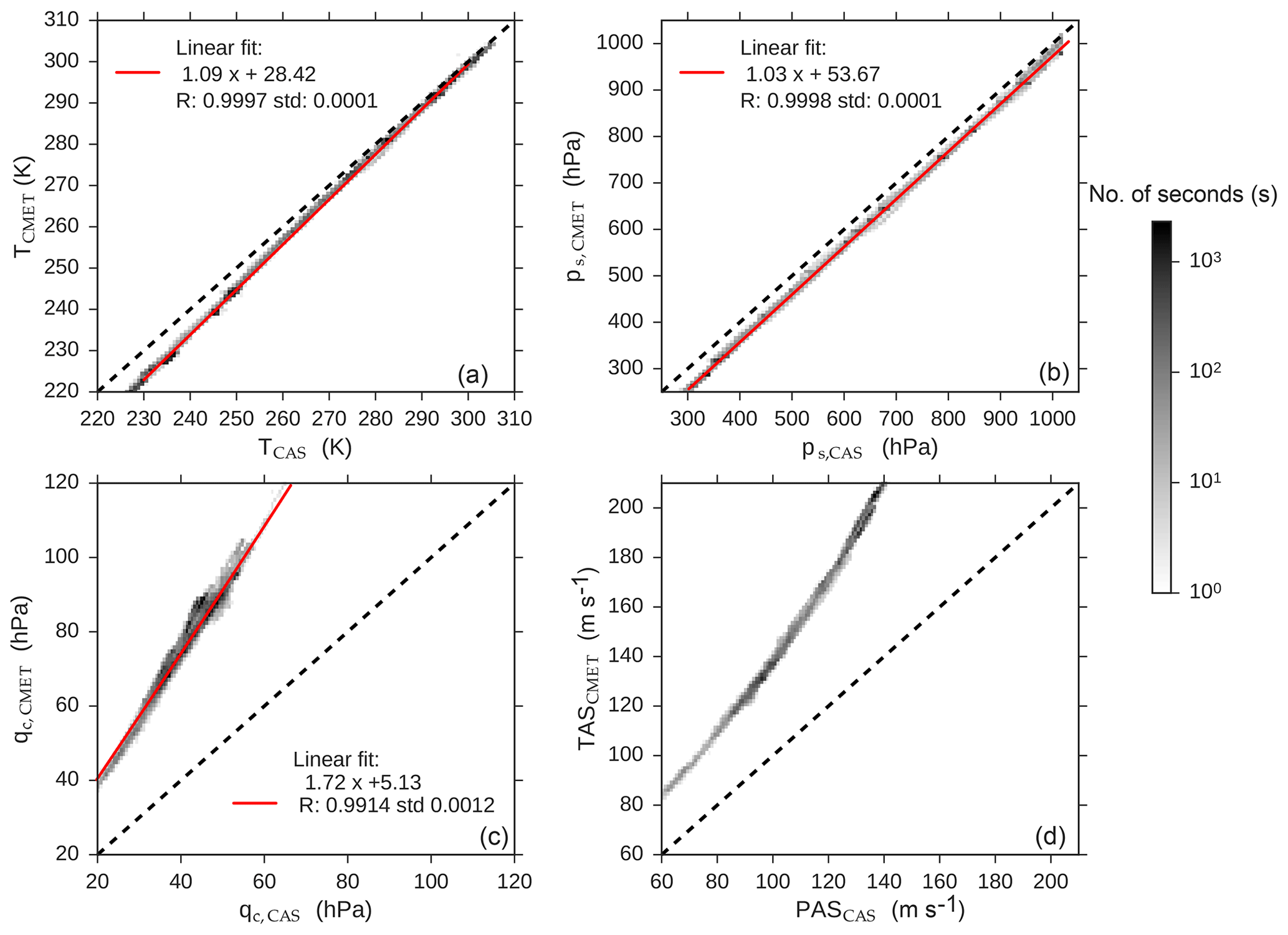
Figure 2 Statistical comparison between values recorded by the CMET system and the CAS pitot tube during SALTRACE: temperature (a), static pressure (b), dynamic pressure (c), and air speed (d). The histogram color map refers to the number of seconds of data at 1 Hz. Dashed lines represent the 1:1 line and the red lines linear fits.

The CAS is equipped with a 17 cm pitot tube, whereas the CAPS has a 24 cm long one to represent the conditions in the CIP sampling area. Pressure sensors have been statically calibrated by the manufacturer. Comparisons of the total pressure p_tot measured by the pitot tube of the wing-mounted instrument (CAS or CAPS) with corresponding measured p_tot of the aircraft system (CMET or MMS) reveal deviations of less than 2 %. Therefore, the position error can be estimated using the deviations between the CMET or MMS measurements, representing the free stream conditions, and the wing-mounted instrument reading. Figure 2 shows a statistical comparison between temperature (a), dynamic pressure (b) and static pressure (c) values recorded by the CMET system at the nose boom (free stream) and by the CAS instrument during SALTRACE. In Fig. 2d TAS_CMET is compared with the PAS calculated using the pitot tube data according to Eq. (3). Pixels are color coded with the statistical frequency of the binned data. Red lines in Fig. 2a–c are linear fits of the data with calculated R² values.

As indicated by the deviation from the 1:1 line (dashed), wing-mounted instruments experience an overpressure on their static sensors (Fig. 2b). Since the total pressure is constant along the aircraft (within the pressure sensors errors), a higher static pressure p_s results in a lower dynamic pressure q_c (Fig. 2c). Consequently, the calculated PAS is on average 30 % lower than TAS, with a 35 % maximum relative deviation at higher speed (Fig. 2d). In the Appendix, analogous comparisons of static pressure p_s and dynamic pressure q_c measured by CAPS and the DC-8 MMS system are shown for ATom-1 (Fig. A1). To understand the differences between PAS and TAS, we use a numerical model.

2.2 Numerical models

2.2.1 Flow model

As mentioned earlier, the assumption of incompressibility of air is not valid for fast-flying aircraft (M>0.3) such as the DLR Falcon and the NASA DC-8. A more general model including air compressibility is needed. Here, we use a numerical CFD model based on the time-averaged Navier–Stokes equation for compressible flows (Johnson, 1992). The numerical solution is obtained using a modified version of the rhoSimpleFoam solver from the finite volume code OpenFOAM v4.0.x (Weller et al., 1998). The solver calculates a steady state solution with a segregated approach using a SIMPLE loop, with the latter solution solved using the Reynolds-averaged Navier–Stokes equations (RANS) with a LaunderSharmaKE (Launder and Spalding, 1974) turbulence model. Nakao et al. (2014) successfully used OpenFOAM for simulating the airflow on a two-dimensional NACA (National Advisory Committee for Aeronautics) wing profile under different attack angles.

In our study, we use a simplified three-dimensional model of the Falcon wing equipped with a probe measurement system, which consists of a pylon and a cylindrical canister mounted under the wing (see Fig. 1). The tube of the CAS with the passive inlet was not modeled since preliminary simulations showed that the effect of the CAS tube on the concentrations measured by CAS is smaller than 5 %. For simplicity, we reduced the complexity of the parameter space using a constant angle of attack of 4^∘ which is the median value derived from the flight conditions (see Figs. A2 and A3 in the Appendix). We adopt a comparatively large model domain with edge lengths of 10 times the instrument length to minimize the effects of the domain boundaries. The model mesh comprises 8×10⁶ elements. The dependency of the results on the number of mesh elements was tested, using different meshes (created with snappyhexmesh Montorfano, 2017), until we found convergence of the results. To separate CFD results from the statistical analyses conducted over the measured dataset we refer to the simulated velocity as U being the absolute value of the three-dimensional velocity vector. U₀ is the velocity in the free stream of the simulations. With this notation U₀ is equal to TAS.

Note that the aircraft fuselage was not included in the model domain because of limitations of computational resources and its limited effect on the flow at the mounting point of the CAS (1.5 m distance from the fuselage during SALTRACE) as shown below in Sect. 3.1.1. Different aircraft types, e.g., DC-8, or different mounting locations may affect the airflow at the instrument. However, as will be shown below, our flow model, with the CAS mounted on the Falcon wing, can be used for general conclusions because particle concentrations depend only on the ratio between the local airflow and the free stream airflow.

2.2.2 Particle motion

To describe particle motion, we adopt an Eulerian–Lagrangian approach: the Eulerian continuum equations are solved for the fluid phase (see Sect. 2.2.1), whereas Newton's equations describe the particle motion determining their trajectories. We assume spherical particles with a density ρ_p=2.5 g cm⁻³ for mineral dust and ρ_p=1 g cm⁻³ for water droplets. We use a one-way coupling; i.e., we consider flow-induced drag forces on the particles. According to Elghobashi (1991), ignoring the effect of particle motion on the flow itself (two-way coupling) and inter-particle collisions (four-way coupling) is a reasonable assumption for volumetric particle fractions smaller than 10⁻⁶. For dust particles, this corresponds to atmospheric concentrations lower than 2.5 g m⁻³. This value is at least 2 orders of magnitude larger than concentrations measured in dense desert dust aerosol layers (e.g., Kandler et al., 2009; Weinzierl et al., 2009, 2011; Solomos et al., 2017) or volcanic ash layers (e.g., Barsotti et al., 2011; Poret et al., 2018). Single particle motion is resolved using a Lagrangian model where motion equations are integrated in time. The considered forces acting on a particle are the pressure gradient, the drag force, and the gravity.

2.2.3 Droplet distortion model

As described in the introduction, fast changes in the airflow can modify the shape of water droplets causing droplet breakup and consequently strongly affecting the measured number concentration. Here, we use a droplet deformation model to describe how the flow affects the shape of water droplets measured by OAP instruments mounted under-wing. A large body of research exists on droplet deformation and breakup (Rumscheidt and Mason., 1961; Rallison, 1984; Marks, 1998). The droplet dynamics is crucial for estimating the icing hazard of supercooled droplets on an aircraft wing (e.g., Tan and Papadakis, 2003). Flow changes experienced around the wing can have important consequences especially when sampling supercooled droplets, for example, in the case of mixed-phase clouds. Jung et al. (2012) observed how shear could cause almost instantaneous freezing in supercooled droplets. Vargas and Feo (2010); Vargas (2012) used laboratory observations to investigate the deformation and breakup of water droplets near the leading edge of an airfoil. Droplet breakup, as an effect of the instability caused by shear on the droplet surface, was early studied by Pilch and Erdman (1987) and Hsiang and Faeth (1992). Different analytical models exist for describing a droplet in a uniform flow such as the Taylor Analogy Breakup (TAB) model (O'Rourke and Amsden, 1987), Clark’s model (Clark, 1988) and the droplet deformation and breakup (DDB) model by Ibrahim et al. (1993). Vargas (2012) modifies the DDB model to include the effect of a changing airflow. However, this model does not fully agree with the experimental data especially for particles with diameters larger than 1000 µm. Here we use a volume of fluid (VOF) method (Noh and Woodward, 1976) to determine droplet deformations as a function of droplet size and flight conditions (p_s, T, TAS). Droplets are initially assumed to be spherical with diameter d₀. Similar to the TAB model a simplified problem is considered assuming that droplets are radially symmetric along the flow.

Sampled droplets experience a change of slip velocity U_slip (speed of particle relative to the air around it) when approaching the instrument. For this reason, we simulate a transitional state where the air speed varies from zero (still air) to its final value TAS minus PAS (when the droplet is passing through the sampling area). The applied velocity values are calculated along the simulated trajectory of the droplet (of given d₀) and imposed as boundary conditions. Similar to Vargas (2012) we assume that the droplet does not exchange heat with its surroundings and the only forces involved in the deformation of the droplet are viscous, pressure and surface tension forces.

The numerical method relies on the solver InterFoam included in OpenFOAM. Numerical schemes for solving the flow are second-order implicit schemes both in the spatial and in the temporal discretization (Rhie and Chow, 1982). The Courant number, i.e., the flow speed multiplied by time resolution and divided by space resolution, is limited to 0.8 globally and to 0.2 at the interface, and the domain size is 10 times larger than the droplet, as suggested by Yang et al. (2017). The simulations have been performed with a water to air density ratio of 1000:1. Surface tension decreases with temperature from σ=0.75 N m⁻¹ at T=278 K to σ=0.70 N m⁻¹ at T=305 K (Vargaftik et al., 1983). The effect of a change in droplet surface tension due to the presence of impurities is not considered which seems to be a reasonable assumption given that salts increase the surface tension of seawater only by less than 1 % (Nayar et al., 2014).

3 Results and discussion

3.1 Airflow distortion, particle concentration, and OAP reference speed

Aerosol concentrations are usually expressed as particle number (or mass) per unit volume. Since the aerosol particles are embedded in the air, and the air density depends on pressure and temperature, the aerosol concentration depends as well on these parameters. Therefore, sampling conditions, e.g., the flight level pressure or the flow-induced pressure distortion at the measurement location, influence the concentration measurement directly.

Table 2 Flight conditions (p_s, T, TAS) used to initialize the numerical flow simulation test cases.

Figure 3 A 2-D histogram of flight conditions (pressure and TAS) recorded at 1 Hz by the CMET system at the nose boom during SALTRACE. Pixels are color coded with the number of seconds spent in the corresponding condition. Colored dots represent the selected test cases for the CFD investigations described in Table 2.

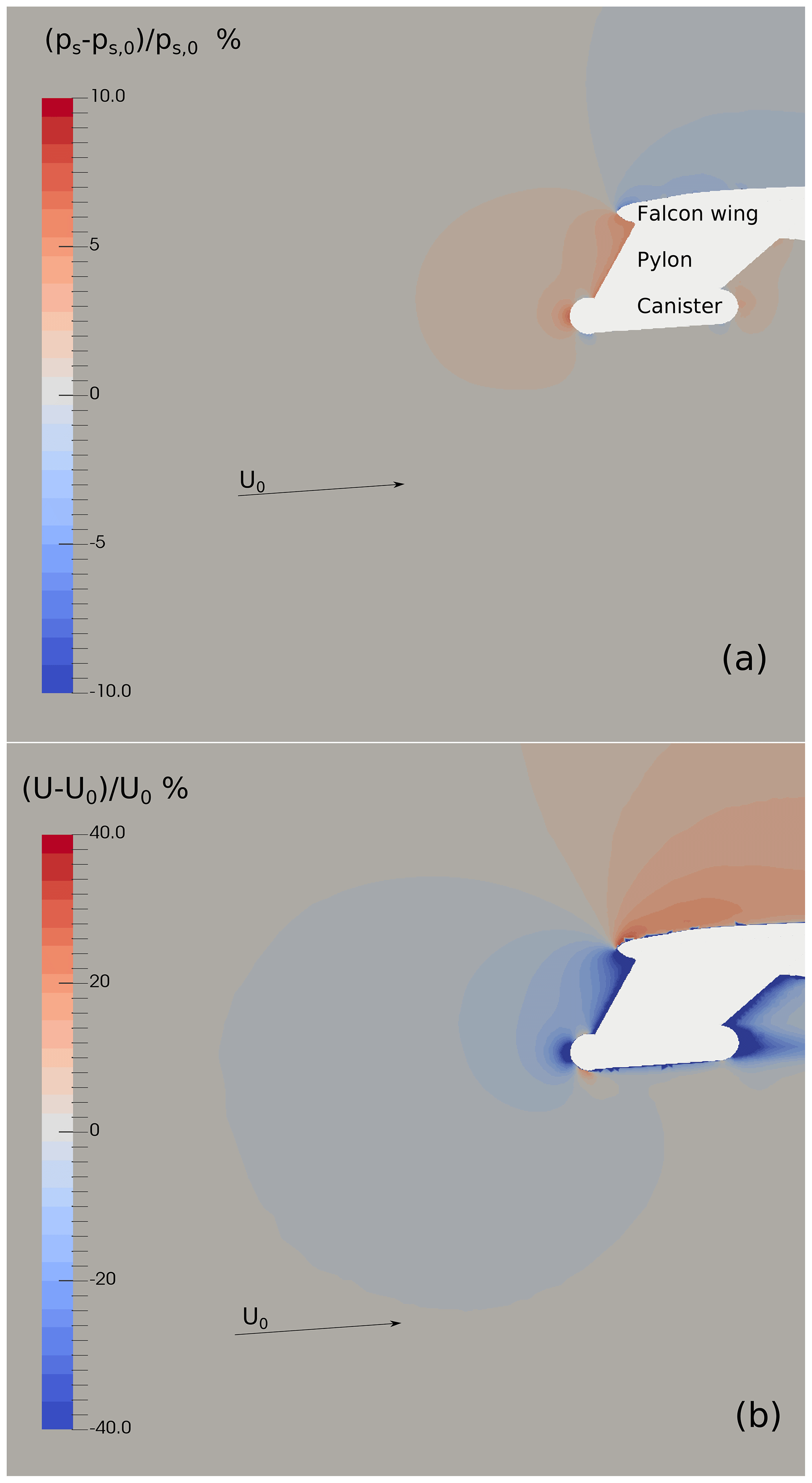
Figure 4 Vertical slice through the probe center and along the flow direction for the simulated test case u100_p900. The white area represents the aircraft wing with the pylon and the probe installed. Colored contours illustrate the static pressure p_s (a) and the velocity field (b) expressed as the ratio compared to the free stream values. The overpressure in front of the probe is slowing down the flow field.

3.1.1 Measured and simulated airflow

To understand the effect of different flight conditions on the measurements, we selected 11 test cases (see Table 2) for the simulations with initial data (p_s, T, TAS) chosen from flight conditions recorded during SALTRACE. Figure 3 shows a frequency histogram of the static pressure p_s and the TAS recorded by the CMET system during the SALTRACE campaign. The colored dots represent the 11 selected cases. Only certain combinations of p_s and TAS represent typical flight conditions for the DLR Falcon. For example, low pressure (high altitude) is associated with higher aircraft speed (when air density is lower, the aircraft needs to fly with a higher speed to have the same lift). As an example for all test cases, we first analyze the result for the specific test case u100_p900 (TAS =100 m s⁻¹ and p_s=900 hPa; see Table 2). Figure 4 shows the simulated airflow in a vertical plane through the Falcon wing where the simplified probe is mounted (white region). The local pressure (a) and the local air speed (b) are expressed as relative deviations (in percent) from free stream conditions. During flight, the pressure above the aircraft wing is lower than in the free stream, while the pressure below the wing is higher, resulting in a lower air speed at the wing-mounted probe compared to free stream conditions (Fig. 4b). Pressure and velocity changes in front of an obstacle are a function of the distance from the obstacle. In the case of an incompressible flow, Stokes provided an analytical expression for the velocity field in front of a sphere. However, in the case of a compressible flow, a necessary assumption for a fast-flying aircraft (TAS>150 m s⁻¹), analytical solutions have not been found yet. Figure 5 shows the ratio between the local conditions near the probe and free stream conditions for pressure (a) and air speed (b) as a function of the distance from the instrument head. The different colors represent a selection of test cases with different TAS (increasing from light-blue to brown). The gray round shape symbolizes the simplified instrument mounted in a canister below the aircraft wing. The pitot tube is sketched in dark gray. The location of the static port is marked with a vertical red line, whereas the location of the tip of the pitot tube is marked with a light gray line. Note, that the sampling area of the instrument is located at the same horizontal distance from the instrument head as the tip of the pitot tube, thus conditions at the light gray line should be representative of the location of the aerosol measurement. Contrary to the incompressible case, where the ratio U∕U₀ is independent of the air speed U₀ (TAS), here due to compressibility the ratio is changing with U₀. An incompressible case in Fig. 5b would be similar to the u75_p1000 simulation where the compression effect is still small. As visible in this figure, the relative air speed difference between the free stream and the instrument location increases with TAS.

Figure 5 Static pressure and velocity normalized by the free stream values calculated along a streamline as a function of the distance from the instrument head. Different colors represent different tests described in Table 2. The gray area marks the pitot tube location, while the red area marks the static port location. The pitot tube was designed to measure the pressure conditions representative of the sampling area of the instrument.

Errors in the pressure measurement can arise due to the position of the static port relative to the tip of the pitot tube. For a pitot tube in a laminar flow, errors are a function of the pitot tube length and the static port distance from the tip (Barlow et al., 1999). For CAS, the static port is located 44 mm downstream of the tip. According to Fig. 5a this difference will lead to a deviation in the pressure since the pressure is decreasing exponentially as a function of the distance from the probe head. However, these differences are still small compared to the position error. For example, considering the numerical test case u100_p900 (see Fig. 5), a CAS pitot tube reading will overestimate p_s by 2.5 % and underestimate air speed by 26 % as compared to the free stream values.

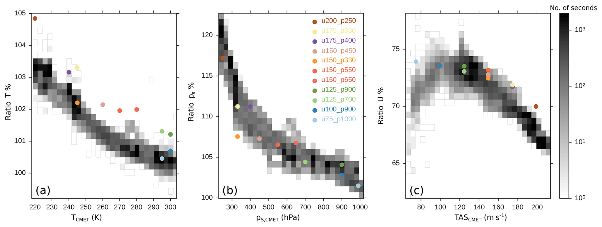
Figure 6 Statistical analysis of ratios between values read by the CAS pitot tube and the CMET system during SALTRACE. The histogram color map refers to the number of seconds of data at 1 Hz. Colored dots represent the selected test cases for the CFD simulations described in Table 2.

To understand the differences between the free stream conditions and the conditions at the wing-mounted instrument, we analyzed the data collected during SALTRACE and compared them with the results from the numerical simulations. Figure 6 shows a statistical analysis of ratios between values read by the CAS pitot tube and the CMET system during SALTRACE for temperature (a), static pressure (b) and air speed (c). The histogram color map refers to the number of seconds of available 1 Hz data of these ratios as function of specific T_CMET, p_s,CMET, TAS_CMET. The different marker colors indicate the selected simulation test cases described in Table 2. The simulation results in Fig. 6 are valid for the pitot tube static port location. The temperature difference between free stream conditions and the probe is decreasing from 3.5 % to 0.5 % with increasing temperature. This effect is a response to a lower aircraft speed at low altitude (see Fig. 3). Also, the trend of the pressure difference in Fig. 6b shows a similar behavior decreasing from 20 % at high to 1 %–2 % at low altitude. Local conditions differ from free stream also for air speed as shown in Fig. 6c with air speed being 25 % to 35 % lower at the probe location compared to the free stream. In this context, it is worth mentioning that a longer pitot tube, as in the case of CAPS (as compared to the CAS used during SALTRACE), will reduce the position error because the deviation of the pressure in front of the probe from the free stream pressure is exponentially decreasing with increasing distance from the probe head. Indeed, the differences between TAS_CMET and PAS_CAPS are only 15 % to 20 % (see the Appendix, Fig. A4).

The simulated conditions at the pitot tube location well represent the measured data from the SALTRACE campaign with small deviations (see Fig. 6). These comparisons indicate that our simplified instrument model geometry and the exclusion of the fuselage in the simulations introduce an uncertainty of less than 5 %. The deviation of U for u75_p1000 (Fig. 6c) from the measurements may be related to changes of the aircraft configuration at low altitude when the flaps are used. The systematic differences in temperature (Fig. 6a) need a separate explanation. Like pressure also the temperature is increasing near the probe head. For this reason, temperature measurements are sensitive to the measurement location. In the CAS and CAPS instruments, the temperature sensor is installed in the back (see CAPS photograph in the Appendix, Fig. A5), and the temperature measurement is corrected using the Bernoulli equation to obtain the temperature at the pitot tube. Consequently, errors in pressure will lead to an error in the temperature. This provides a possible explanation for the 1 % difference between the temperature values obtained from the instrument and the simulations (Fig. 6a). The temperature bias is probably due to a combination of static pressure bias, instrumental uncertainty, and model parameterization. Nevertheless, an error of 1 % in T will lead, according to Eq. (3), to a PAS error of about 0.5 %. Thus, the uncertainty of the temperature has only a very small contribution to the uncertainty of the PAS and is therefore negligible.

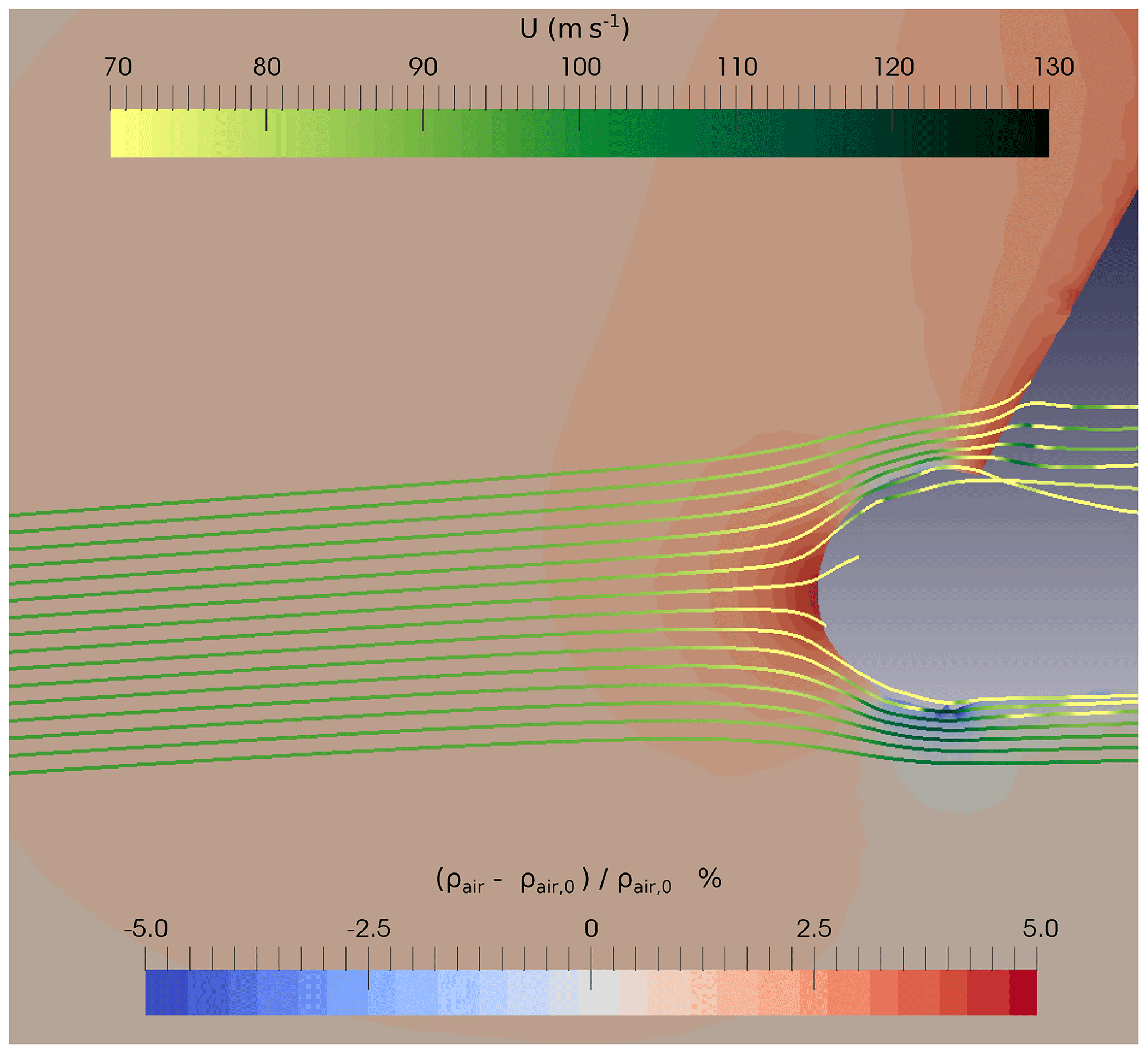
Figure 7 Relative deviation of air density ρ_air around the probe from the air density ρ_air,0 in the free stream for the test case u100_p900 as contours in the background (color code at the bottom). Lines in the foreground represent streamlines colored with the local airflow velocity U (color code at the top).

Figure 8 Sampling efficiency calculated as a function of modified Stokes number (see Eq. 4) for selected numerical test cases of Table 2. Each marker represents a run where we released 2×10⁵ particles of a specific diameter (colors) and density (dust: squares; water: circles) in front of the probe in the computed flow field. Sampling efficiency is defined as the ratio between particles released and particles passing through the sampling area, renormalized by the corresponding areas. Curves are obtained by fitting the data with a sigmoid function (see text).

3.1.2 Simulated particle concentration and sampling efficiency

In this section, we use simulated flow fields (Sect. 2.2.2) to study how the airflow around a wing-mounted instrument affects the particles. For each class of particles with a different density ρ_p and diameter d_p, we release 2×10⁵ particles upstream the instrument at the domain border and calculate the sampling efficiency f_eff as the ratio between particles passing through the sampling area and particles released at the domain border. Counting the particles is done using a Gaussian kernel that reduces the dependency of the estimated particle concentration on the computational grid (Silverman, 1986). These numbers are normalized by the ratio of the releasing area to the sampling area. Figure 7 shows an example of streamlines around the wing-mounted instrument. Contours are color coded with density ρ_air and streamlines with air speed U. Air speed decreases in the vicinity of the probe and streamlines are bent due to the flow distortion caused by the overpressure. This effect has been observed already by King (1984). The ability of particles to adapt to flow changes is expressed by the Stokes number Stk. The Stokes number represents the ratio of particle's response time to the characteristic fluid timescale. Particles with a small Stokes number react immediately to flow changes and consequently follow the streamlines, as in the case of submicron-sized particles. To generalize the analysis according to Israel and Rosner (1982) into the non-laminar flow regime, we use instead of the original Stokes number Stk a modified Stokes number Stk^*, which is defined as

$$\begin{array}{}\text{(4)}& St{k}^{*}={\displaystyle \frac{{\mathit{\rho }}_{\mathrm{p}}U{d}_{\mathrm{p}}^{\mathrm{2}}}{L\mathrm{18}{\mathit{\mu }}_{\mathrm{air}}}}\mathit{\psi }\left(R{e}_{\mathrm{p}}\right)\text{where}R{e}_{\mathrm{p}}={\displaystyle \frac{p_{\mathrm{s}}U{d}_{\mathrm{p}}}{T{\mathit{\mu }}_{\mathrm{air}}{R}_{\mathrm{s}}}}.\end{array}$$

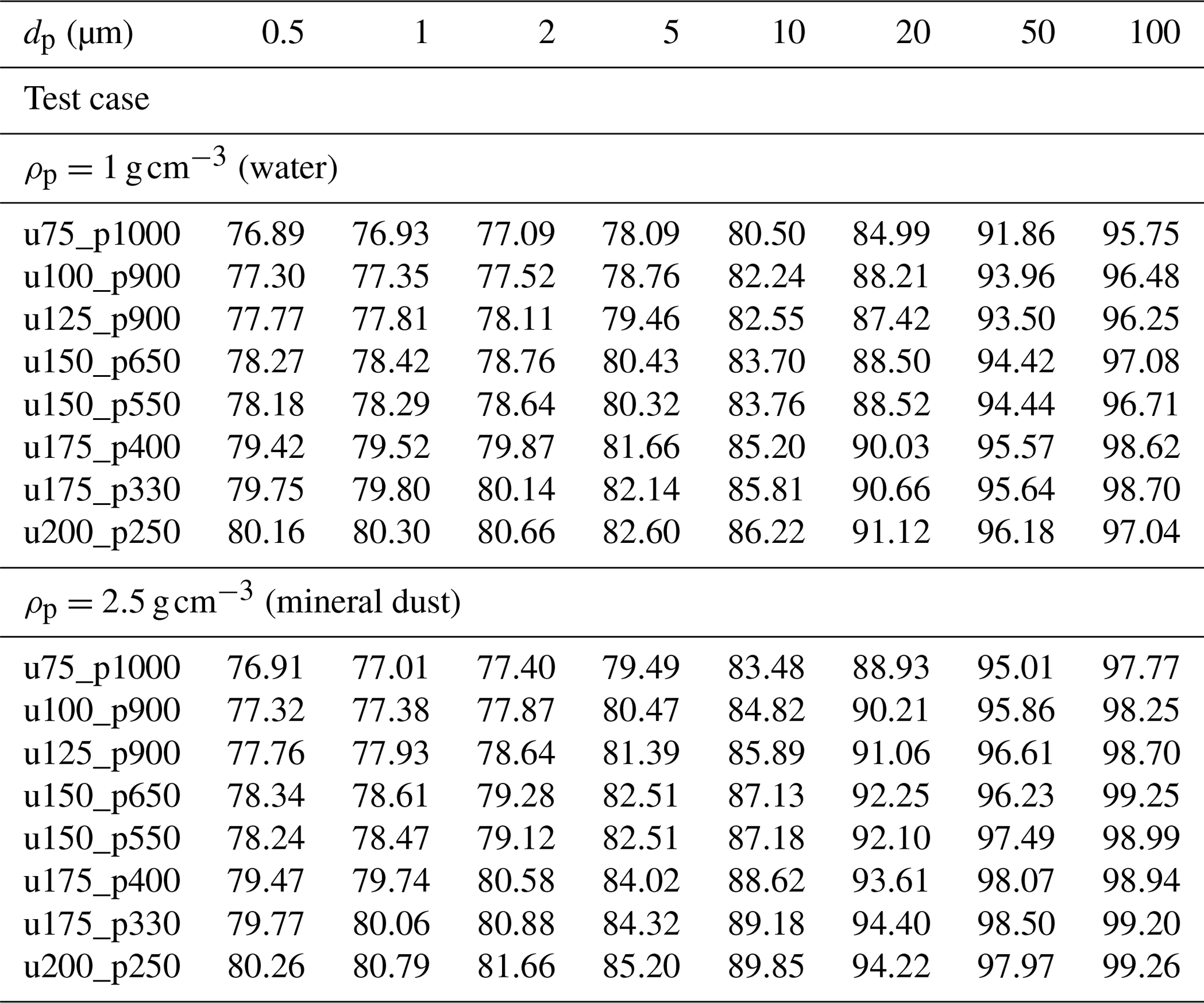
μ_air is the dynamic viscosity of air, R_s is the specific gas constant of air (287.1 $\mathrm{J}{\mathrm{kg}}^{-\mathrm{1}}{\mathrm{K}}^{-\mathrm{1}}$) and ψ the additional correction factor as a function of particle Reynolds number Re_p varying from 1 in the laminar case to values smaller than 0.1 in the case of fully turbulent flow (see Fig. 3 of Israel and Rosner, 1982 or Eq. 36a of Wessel and Righi, 1988 for ψ(Re_p)). L is a characteristic fluid length, here fixed to 1 m. The TAS is used for U in Eq. (4). Figure 8 shows the sampling efficiency as a function of the Stokes number Stk^*. Different symbol colors represent particle diameters whereas the differently colored lines represent fits of sigmoid functions to the Stokes numbers of the selected test cases. The sampling efficiency f_eff is well approximated by the sigmoid fits. In the Appendix, Table A3 presents the sampling efficiencies of the selected test cases for different particle diameters and densities. For large Stokes numbers, the simulated droplet concentration at the probe is minimally affected by the flow. For example, f_eff>95 % holds for diameters larger than 100 µm. For small particles with less inertia, the effect caused by the flow is more evident, and it leads to a sampling efficiency of ∼77 % (test case u100_p900). This effect appears less marked for test cases at higher TAS and lower pressure, e.g., for u200_p250, where 80 % of the small particles reach the sampling area. It is worth mentioning that simulations considering only the wing itself without the instrument (not shown) result in f_eff values around 91 %–92 % for small Stk^* illustrating that both the wing and the instrument affect the flow at the sampling location.

Figure 9 Particle velocity v_p normalized by PAS_CAS (a) and TAS_CMET (b) as a function of modified Stokes number Stk^*. The contour thickness of the markers increases with TAS. Colors denote particle diameters.

The change of particle inertia as a function of particle diameter plays a significant role also for particle velocity. As King (1984) reported, particle speed v_p may significantly differ from the local air speed depending on their Stokes number. Figure 9 shows the particle speed v_p normalized by PAS (a) and TAS (b) for the selected test cases. Different colors represent different particle diameters and marker thickness is a function of the TAS. For each simulated case, particle speed is calculated as an average of the sampled particles. For diameters smaller than 5 µm, PAS is a reasonable approximation of particle speed. Larger particles with a higher Stokes number, are less influenced by the airflow change due to their inertia. For this reason the particle velocity v_p for diameters d_p>50 µm can be well approximated using the TAS with an error smaller than 10 % (see Fig. 9b). Figure 9b also shows that at higher TAS (see gray arrow) the normalized particle speed is lower, especially for smaller particles, because of the lower normalized air speed (Fig. 5).

3.1.3 Compressibility effect on particle concentration: a correction strategy

The PAS is lower than TAS (during SALTRACE, PAS/TAS ≃70 %; see Fig. 6c). Thus, for a given number of particle counts per time interval, particle number concentrations calculated using PAS as a reference speed are larger than values obtained using TAS. Furthermore, the temperature and the pressure at the probe are higher than in the free stream as shown in Fig. 6a and b. Wrong temperature and pressure values will lead to errors of the concentration values after conversion to other conditions, e.g., those in the free stream. A higher pressure value leads to a lower calculated concentration, whereas it is directly proportional to the temperature value used.

Weigel et al. (2016) provide a method to derive ambient number concentration from data of underwing instruments that is primarily based on the concept that the air compression near the instrument causes a corresponding densification of the number concentration of airborne particles. Subsequently, they take into account a size-dependent correction factor that corrects the effect of the inertia of large particles. Their inertia correction is mainly assessed on the basis of the circularity of droplet images taken by an OAP at a resolution of 15 µm. Weigel et al. (2016) conclude that particles with diameters d_p<70 µm follow the airflow and thus require no inertia correction. On the contrary, our simulations (see, e.g., Fig. 9) show a notable impact of the particle inertia already for particle diameters d_p=10 µm (their speed is about 10 % higher than the air speed; particle density 1 g m⁻³) and a strong impact for 50 µm particles (about 25 % faster than air). These particle simulations are consistent with results (not shown) from a simplified numerical particle motion model using the simulated flow fields (Sect. 3.1.1) as input and Eq. (3.5) of Hinds (1999) (which is based on Clift et al., 1978) to calculate the drag force on the particles. Therefore, we conclude that inertia needs to be taken into consideration for particles larger than about d_p>5–10 µm.

The main idea of our concentration correction strategy is to express the sampling efficiency f_eff as a function of the Stokes number and a parameter α describing the difference between the probe and the free stream conditions:

$$\begin{array}{}\text{(5)}& \mathit{\alpha }={\displaystyle \frac{p_{\mathrm{s},\mathrm{probe}}}{p_{\mathrm{s},\mathrm{free}}}}{\displaystyle \frac{T_{\mathrm{free}}}{T_{\mathrm{probe}}}}{\displaystyle \frac{\mathrm{PAS}}{\mathrm{TAS}}}.\end{array}$$

Using α as variable, the sampling efficiency f_eff (in %) can be approximated with the sigmoid equation:

$$\begin{array}{}\text{(6)}& f_{\mathrm{eff}}(\mathit{\alpha },St{k}^{*})=k_{\mathrm{0}}+{\displaystyle \frac{\mathrm{100}\mathit{\%}-k_{\mathrm{0}}}{\mathrm{1}+e^{k_{\mathrm{1}}}\cdot (St{k}^{*}{)}^{k_{\mathrm{2}}}}}.\end{array}$$

The sampling efficiency values from the simulations for different flight conditions and for different distances from the probe were used to fit the coefficients in Eq. (6), finding $k_{\mathrm{0}}=\mathrm{83.7}\mathit{\%}\cdot \mathit{\alpha }+\mathrm{14.6}\mathit{\%},k_{\mathrm{1}}=\mathrm{1.86}\cdot \mathit{\alpha }-\mathrm{3.66}$, and $k_{\mathrm{2}}=-\mathrm{0.87}$. Equation (6) allows correcting particle concentrations as a function of the modified Stokes number and flight conditions. For each particle diameter d_p, the first step of the correction is to estimate the corresponding modified Stokes number (Eq. 4) using free stream conditions (p_s, T, TAS) and a range of particle densities. Secondly, the sampling efficiency f_eff is calculated using the Eq. (6). Finally, the ambient number concentration N_i in each diameter bin i (covering the diameter interval from d_p,i to $d_{p,i+\mathrm{1}}$) is calculated as follows:

$$\begin{array}{}\text{(7)}& N_i={\displaystyle \frac{\text{number of detected particles in bin}i}{\text{size of sampling area}\cdot \text{TAS}\cdot \text{measurement duration}\cdot f_{\mathrm{eff}}\left(d_{\mathrm{p}}\right)}}.\end{array}$$

Note that Eq. (6) is an extension of the formula by Belyaev and Levin (1974) where the deviation of the sampling efficiency from unity was found (via a direct method) to be a sigmoid function of the Stokes number and to be proportional to (PAS/TAS – 1).

Figure 10 compares estimated sampling efficiencies with sampling efficiencies obtained directly from the simulations. Two different estimation methods are considered to illustrate the benefit of the new correction strategy proposed here. In the “old method” (Fig. 10a) concentrations are calculated using PAS as reference speed, which are then corrected with an adiabatic expansion between the probe and free stream conditions. In contrast, the “new method” (Fig. 10b) uses TAS as reference speed and the fitted sampling efficiency f_eff sigmoid function from Eq. (6). The concentrations calculated with the “old method” are correct for describing the behavior of small particles (see Fig. 10a). Small particles exhibit enough mobility to follow the airflow. In contrast, using probe conditions (PAS) and an adiabatic expansion overestimates the particle number concentration by up to 25 % for coarse-mode particles (d_p>2 µm). This difference will grow even larger if PAS deviates more from TAS. The “new method” (Fig. 10b) shows good agreement with deviations smaller than 2 % for the complete size range. The “new method” not only has the advantage of reducing concentration errors but it also reduces the size dependence of these errors.

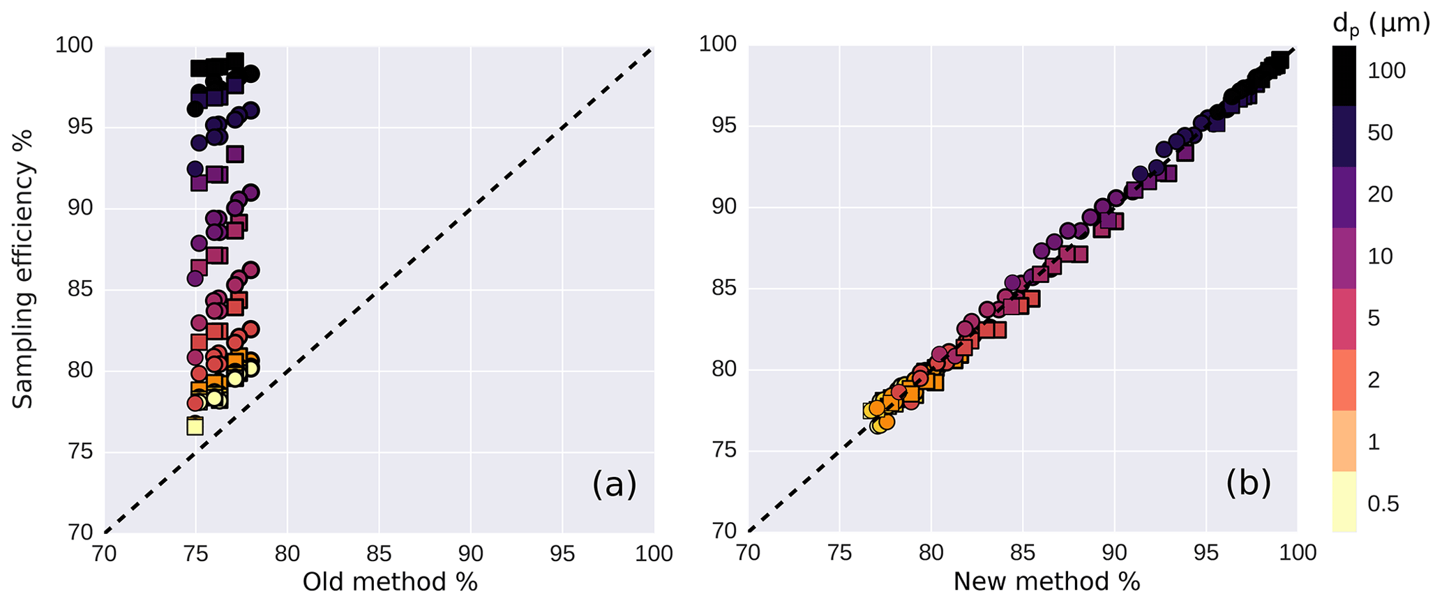
Figure 10 Simulated sampling efficiency f_eff versus sampling efficiencies estimated from the simulations using the “old method” (a) and the “new method” (b). Different markers indicate different numerical test cases, while the colors refer to the particle diameter. For the “old method”, the concentration is calculated using the probe conditions and using an adiabatic expansion to free stream conditions. For the “new method”, the concentration is calculated using free stream conditions and corrected for the flow distortion by applying Eq. (6). To obtain the sampling efficiency, concentrations from both methods are divided by concentration assumed in the free stream.

3.1.4 Reducing OAP errors related to OAP reference speed

The OAP reference speed is usually derived from measurements with a pitot tube being part of the OAP, thus by default represent local conditions. As explained in Sect. 2.1.1 the OAP reference speed is critical for the correct reconstruction of the particle size in the direction of the flow. OAP instruments mainly cover particle diameters larger than 30 µm. Figure 9b shows that particle speed v_p in this size range is close to TAS, i.e., v_p is minimally affected by the flow around the aircraft. Thus, using the PAS as a OAP reference speed will result in images flattened along the flow direction, with a relative error proportional to the relative offset of PAS from TAS. On the contrary, TAS is a good approximation for the OAP reference speed minimizing image distortion errors. Therefore, the basis of the correction method proposed here is to calibrate the pressure sensors such that the pitot tube of the OAP reports TAS instead of PAS. This can be achieved by performing a similar analysis as presented in Fig. 2. In our case, the CAPS pitot tube was re-calibrated using data from the CMET system together with simultaneous measurements of CAPS during some test flights. A linear fit² between the free stream conditions from the CMET system and the probe conditions from CAPS is performed for q_c and p_s. A similar analysis was conducted using NASA DC-8 data provided by the MMS for ATom-2, ATom-3, and ATom-4.

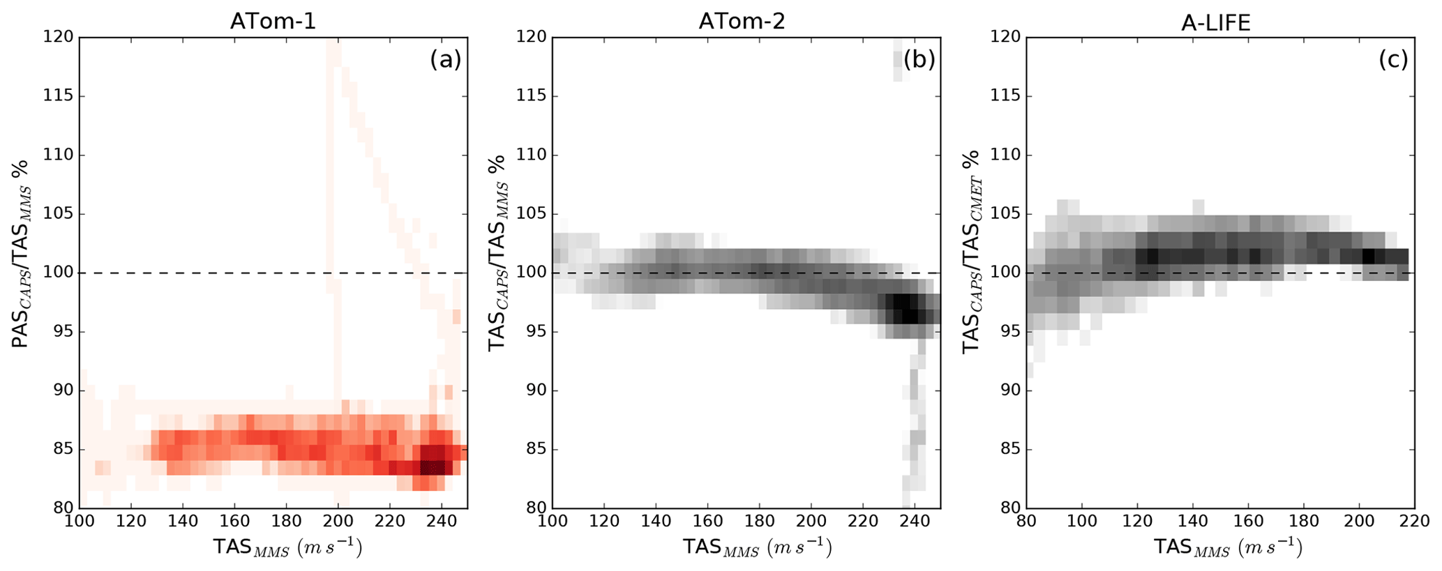
Figure 11 Air velocity recorded by CAPS normalized by air velocity recorded by the default aircraft systems. Data from ATom-1 (a), ATom-2 (b), and A-LIFE (c) are shown. While the CAPS pitot tube was calibrated to match PAS during ATom-1, it was calibrated to match the TAS during ATom-2 and A-LIFE. The pixels are color coded with the number of seconds of data at 1 Hz.

Figure 11 shows the ratio of the air speed reported by the CAPS instrument and the TAS during the NASA DC-8 campaigns ATom-1 (a, 2016), ATom-2 (b, 2017), and the Falcon campaign A-LIFE (c, 2017). Whereas during ATom-1 the CAPS pitot tube calibration was based on the manufacturer settings reporting PAS, the CAPS pitot tube was calibrated to match free stream conditions reporting TAS during ATom-2 and A-LIFE. The obtained air speed during ATom-2 and A-LIFE, named hereafter TAS_CAPS, shows on average a 2 % deviation from the TAS_CMET and 3 % from TAS_MMS. Contrary, during ATom-1, the uncorrected PAS_CAPS shows an offset with the TAS_MMS larger than 15 % (see Fig. 11a).

3.2 Droplet deformation

The recorded shape of droplets using an OAP is a combination of the real particle shape influenced by the sampling conditions and, as discussed above, instrumental effects such as those resulting from the settings to calculate v_p. In the following we evaluate OAP image distortions along the flow direction to estimate the correctness of the assumed particle speed v_p and to investigate aerodynamic effects on the real droplet shape. Since ice crystals mostly present irregular shapes, we limit our analysis to liquid droplet images.

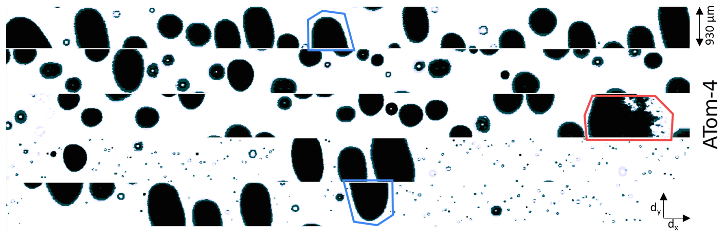
Figure 12 CIP gray-scale images collected in a liquid cloud during the ATom-4 campaign. Colors are the three levels of shadow recorded on each photodetector. The vertical scale is 62 pixels of 15 µm, while the horizontal axis represents the timeline. The red contour indicates splashes due to a droplet breakup. Blue contours highlight examples of large particles that are not fully recorded.

Figure 12 shows sequences of gray-scale images taken with the CIP in cloud passages during the ATom-4 campaign. The vertical dimension (y axis) of these images is the dimension of the optical array (being perpendicular to airflow direction) and the horizontal dimension (x axis) initially is the time dimension, which is converted to length using the OAP reference speed. As discussed, using PAS would result in particles flattened in the horizontal dimension since for particles in the OAP size range v_p is higher than PAS (Fig. 9). For the particles shown in Fig. 12 pressure and temperature conditions recorded during the passages ensure droplets being in a liquid state. Image colors are the three levels of shadow recording on each photo-detector. The vertical scale is 62 pixels, where each pixel represents an area of 15 µm⋅15 µm. Images were taken using the TAS_CAPS as reference speed. TAS_CAPS is obtained as explained in Sect. 3.1.4. The smaller droplet images are nearly circular, whereas larger droplets show deformed shapes, with the deformation becoming increasingly visible with increasing size. The red contour highlights droplet breakup and the blue ones indicate examples of large deformed droplets that are not fully recorded by the array.

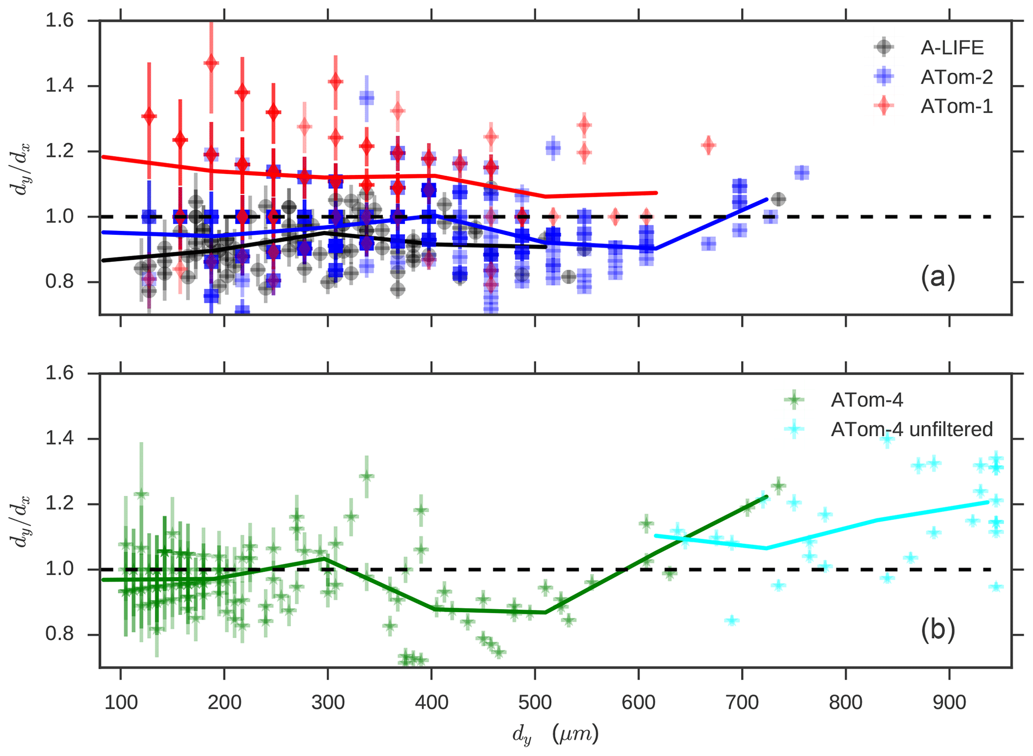
Figure 13 Ratio between the main axis lengths (d_y∕d_x) of droplets recorded by the CIP during different campaigns (indicated by color). Error bars represent the CIP pixel resolution (15 µm). Considered are only particles recorded during cloud passages where the temperature ensures a liquid droplet state. Red markers in the upper panel show data from the ATom-1 mission where the CAPS pitot tube, and thus the OAP reference velocity, was calibrated to match PAS, whereas the data of the other campaigns (shown in dark blue, black, green, light blue) were collected when the CAPS pitot tube was calibrated to match TAS (see also Fig. 11). Lines indicate the mean values of each campaign within several wider size intervals. Data from ATom-4 (green), including particles not fully covered by CIP (light blue), are shown in the lower panel.

To better understand the droplet deformation and v_p deviations from TAS we performed a statistical analysis of droplet images. Figure 13 compares the deformation ratio, defined as the ratio between main droplet axes d_y∕d_x for the different droplet images. To extend our analysis, we included datasets collected during different campaigns (as indicated by the marker colors). The images were taken during selected flight sequences where liquid droplets were encountered. Following Korolev (2007), we choose droplet images showing only a small Fresnel effect and entirely contained in the field of view of the CIP, except for the ATom-4 data marked in light blue (Fig. 13b) where also particles which were not fully recorded were included. Image analyses were conducted using the image processing library OpenCV (Bradski, 2000) (using a contours threshold of 0.8). Error bars in both directions are calculated according to the CIP size resolution of one pixel, corresponding to 15 µm and solid lines indicate the mean value of each campaign. Red markers refer to measurements during ATom-1 with the PAS_CAPS set as reference speed for particles. Dark blue markers refer to ATom-2 when the TAS_CAPS was used after re-calibration of the pitot tube (Fig. 11b). In the case of ATom-1 (red markers), the use of the PAS causes a squeezing effect in the images along the flow direction, i.e., $d_y/d_x>\mathrm{1}$ for most droplets. Contrary, during ATom-2, ATom-4, and A-LIFE the ratio d_y∕d_x is more evenly distributed around 1 illustrating the benefit of using TAS_CAPS as reference speed. For small droplets (<150 µm) the large scattering is due to the limited instrument resolution (see error bars). For larger droplets, error bars expressing the instrumental resolution cannot explain the data scattering. The scattering also cannot be explained by air speed errors only. A possible explanation is the instability effect on the surface of the droplets, as presented in Szakall et al. (2009), and discussed below. To better understand these phenomena, we extend our study by using a droplet deformation model.

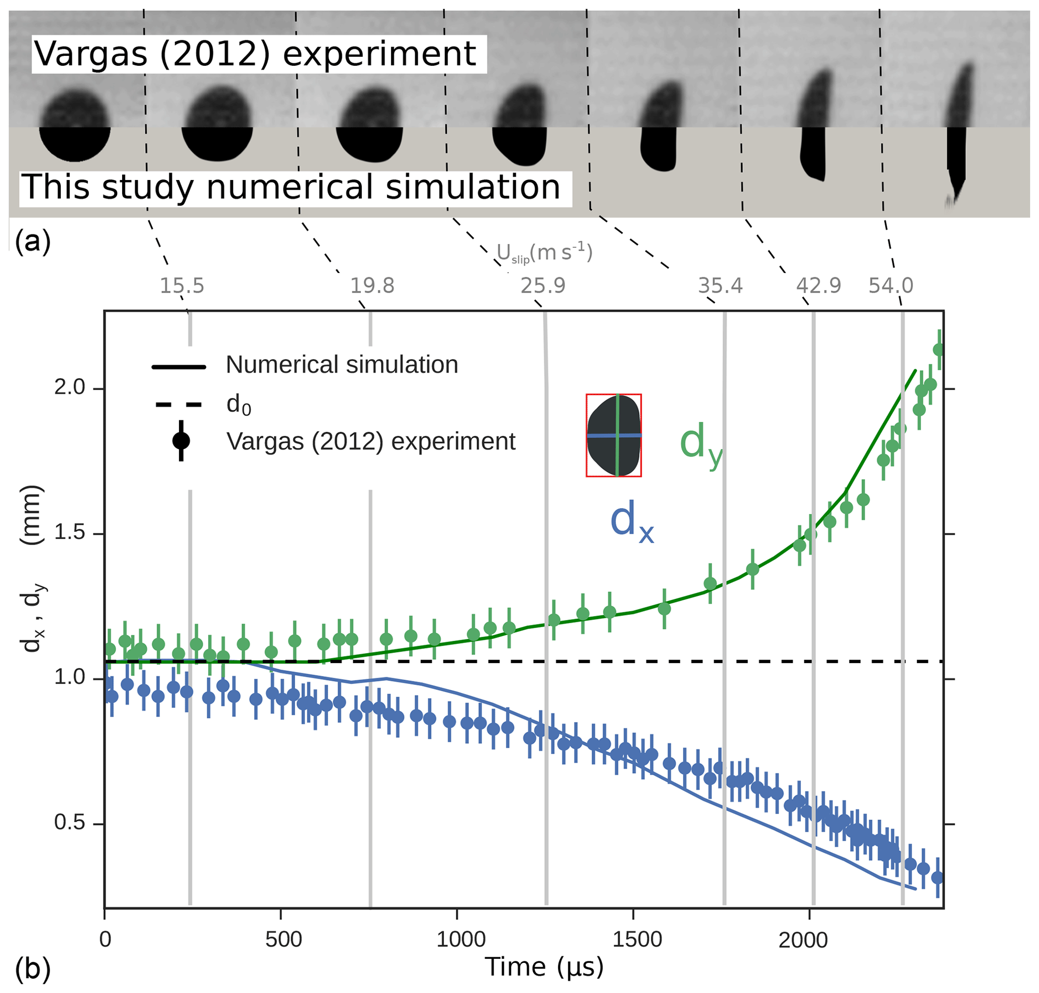
Figure 14 Simulations for a test case with a 1032 µm diameter droplet reproducing an experiment by Vargas (2012). In the upper panel, the upper halves display images recorded by Vargas (2012), while the lower halves show corresponding simulated droplets from the present study. The airflow comes from the left. Time and relative air speed increase from the left to the right. The lower panel shows changes of both droplet axes' lengths (d_x and d_y; see inlay image) as a function of time and relative velocity (labeled at the top) for the experiment from Vargas (2012) (dots) and for the simulations (continuous line).

3.2.1 Quantification of droplet deformation

Before analyzing the results of the droplet deformation model, we test the numerical results by comparison with data from the experimental work of Vargas (2012). We selected the experiments of Vargas (2012) where they observed a 1032 µm water droplet approaching an aircraft wing as test for our simulations. The selected experiment consisted of a droplet that is vertically falling on a horizontally rotating arm with an attached wing profile. The wing profile rotated with a speed of 90 m s⁻¹. In Fig. 14 selected images at different points of time in the Vargas (2012) experiment (upper half of the upper panel) are compared with the corresponding simulation results (lower half of the upper panel). Since the flow circulating around the particle is changing with time, the lower panel also shows the corresponding slip velocity values U_slip defined as the droplet speed relative to the suspending air. To have a more explicit comparison of the change of droplet shape, the lower panel of Fig. 14 shows the lengths of the droplet's axes of the experimental data (dots) and those simulated (lines) as a function of time and relative speed U_slip. The lengths of the axes of individual droplet images are determined using the length and width of a circumscribing rectangle (as sketched in the Fig. 14). As visible in the upper panel, when the droplet approaches the airfoil, U_slip increases and the droplet starts to be squeezed along the flow direction, until the breakup process occurs at the droplet edges for U_slip∼60 m s⁻¹. The model reproduces the behavior of the droplet over time qualitatively well with deviations smaller than 2 times the uncertainties of the experimental data. To extend our result to different droplet diameters and flight conditions, we use the Weber number We which represents the ratio of the aerodynamic forces to the surface tension forces. We is defined as

$$\begin{array}{}\text{(8)}& We={\displaystyle \frac{d_{\mathrm{p}}{\mathit{\rho }}_{\mathrm{air}}{U}_{\mathrm{slip}}^{\mathrm{2}}}{\mathit{\sigma }}}.\end{array}$$

σ is the surface tension and d_p the droplet diameter. In our case, U_slip is changing with time from zero when the droplet is in still air, to its maximum value when the droplet is recorded (U_slip=TAS – PAS for large Stokes numbers).

To understand the data deviation found in Fig. 13 we simulated different droplet diameters. The results are shown in Fig. 15 where the deformation ratio is plotted for the simulated droplets as a function of the We. Different marker colors represent different test cases where we varied droplet diameters. As a droplet approaches the airfoil, the relative speed U_slip increases and therefore the We also increases. The mechanism of droplet deformation and breakup is governed by an interplay of aerodynamic, tension and viscous forces. The distortion is primarily caused by the aerodynamic forces, whereas the surface tension and viscous forces, respectively, resist and delay deformation of the droplet. Gravitational forces play a minor role since the ratio of aerodynamic forces over gravitational forces ${\mathit{\rho }}_{\mathrm{air}}{U}_{\mathrm{slip}}^{\mathrm{2}}/{\mathit{\rho }}_{\mathrm{p}}g{d}_{\mathrm{p}}$, is much larger than unity. When aerodynamic forces grow larger than the surface tension forces, they deform the droplet causing in the worst case a breakup of the droplet by aerodynamic shattering (Craig et al., 2013). For a droplet approaching an airfoil, the viscous forces are smaller than aerodynamic and surface tension forces and the droplet breakup process is mainly controlled by We. Howarth (1963) and Oertel (2010) showed that a droplet requires a critical Weber number (We_crit) for breakup. Wierzba (1990) studied We_crit when droplets interact with an instantaneous airflow in a horizontal wind tunnel. Kennedy and Roberts (1990) studied the breakup of droplets subject to an accelerating flow in a vertical wind tunnel.

Figure 15 Droplet axis ratio (d_y∕d_x) as a function of Weber number (We). Different dots represent different simulations where we increased the initial droplet diameter d₀ from 265 µm (white) to 1062 µm (dark blue). The gray area represents the region where droplet breakup can occur.

The critical Weber number We_crit from different experimental studies with uniform airflow varies around 11±2. Craig et al. (2013) also assumed We_crit=12 for determining the droplet critical diameter d_crit for aerodynamic shattering on an inlet. For a droplet approaching an airfoil, since U_slip is changing and droplets can adjust their shape to the changing flow, droplet breakup occurs at larger We compared to the case of a uniform airflow (Vargas, 2012). On the other hand, the rapid change in the flow creates instabilities and droplets show a deformed shape already at We∼1 (see Fig. 15). Garcia-Magariño et al. (2018) characterized the We_crit providing an analytical equation:

$$\begin{array}{}\text{(9)}& W{e}_{\mathrm{crit}}=\mathrm{17.5}+\mathrm{17.9}\mathit{\tau }\text{where}\mathit{\tau }={\displaystyle \frac{\sqrt{({\mathit{\rho }}_{\mathrm{p}}{d}_{\mathrm{p}}^{\mathrm{3}}\mathit{\pi }/(\mathrm{6}\mathit{\sigma }\left)\right)}}{U_{\mathrm{slip}}/\frac{\partial U_{\mathrm{slip}}}{\partial t}}}.\end{array}$$

Using the simulated airflow fields and Eqs. (8) and (9), we can express the critical diameter d_crit as a function of relative particle speed U_slip. U_slip is a function of TAS and mounting position (see Fig. 5). Therefore, for a specific configuration, d_crit can be expressed as a function of TAS. Figure 16 shows how d_crit decreases when TAS increases. The two colors in Fig. 16 refer to the two different mounting configurations for the DLR Falcon and the NASA DC-8. The difference in the mounting configurations between the Falcon and the DC-8 is the main reason for the differences in the relative particle speed U_slip for a given droplet diameter d_p and TAS, which results in differences in d_crit as shown in Fig. 16. Figure 16 also shows that pressure and temperature have only a rather small effect since results for different test cases with same TAS lie on top of each other. Generally, a large difference between the free stream and the probe air speed will increase the slip velocity U_slip and consequently the Weber number, reducing the critical diameter for droplet breakup. This explains why critical diameters for the Falcon configuration are smaller than for the DC-8.

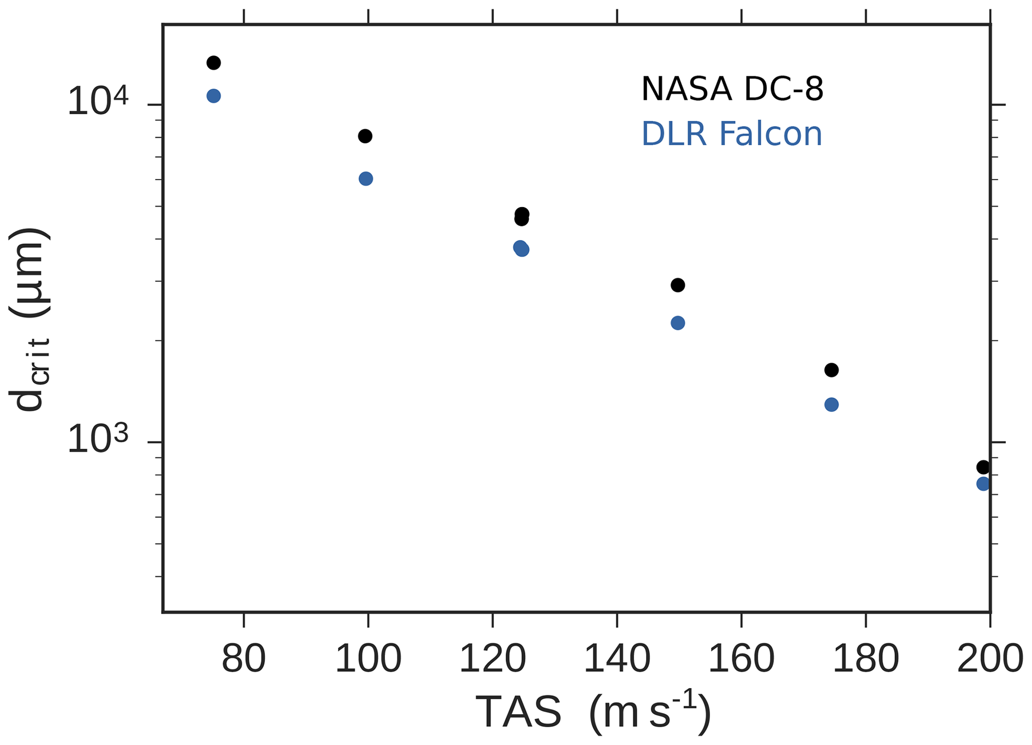
Figure 16 Critical diameter for droplet breakup as a function of TAS for the DLR Falcon and the NASA DC-8 configuration.

In general, smaller droplets resist deformation more than larger ones because the small diameter translates into a larger curvature. However, relatively small droplets can show instability phenomena where the droplet surface starts to oscillate (called Taylor instability) which are not resolved in our simplified droplet model. This effect can be responsible for some additional scattering of data in Fig. 13.

The aerodynamic deformation of larger droplets, as modeled in Fig. 15, is only partially visible in the statistical analysis presented in Fig. 13, since large droplets have a higher chance to be only partially recorded inside the field of view, and consequently being excluded from the study. However, when considering particles not fully recorded inside the field of view, the deformation becomes visible for particles larger than about 600 µm, as shown for the ATom-4 data in Fig. 13b. Most have ratios $d_y/d_x>\mathrm{1}$ going up to 1.4 which is confirmed by the mean values (lines) being larger than unity. Since the y-extension of these particles is not fully covered by the imaging array, the real ratio d_y∕d_x is probably even higher as indicated by the shape of several incomplete droplet images in Fig. 12 (blue contours).

3.2.2 Impact of droplet deformation on particle volume estimation

As observed in Figs. 12, 14, and 15 large liquid droplets show a large distortion with d_y∕d_x values around 2 and larger, when measured with an OAP aboard a fast aircraft. This raises the question which diameter should be used to describe the size of deformed droplets. Different diameter definitions exist (Korolev et al., 1998). Here, we use as approximation diameters d_approx, the maximum diameter $d_{\max }=max(d_x,d_y)$, the mean diameter $d_{\mathrm{mean}}=(d_x+d_y)/\mathrm{2}$, and the area equivalent diameter $d_{\mathrm{equi}}=\mathrm{2}\sqrt{\mathrm{Area}/\mathit{\pi }}$ where Area is the droplet cross section area calculated from the image. Two additional approximations are used: $d_{\mathrm{spheroid}}=(d_x{d}_y^{\mathrm{2}}{)}^{\mathrm{1}/\mathrm{3}}$ derived assuming a spheroid rotated around the x-axis and $d_{\mathrm{asym}}=(\mathrm{4}/\mathit{\pi }\cdot \mathrm{Area}\cdot d_y{)}^{\mathrm{1}/\mathrm{3}}$. McFarquhar (2004) noted that inconsistencies in particle size definitions could have significant impacts on mass conversion ratios between different hydrometeor classes used in numerical models. Errors in the droplet volume approximations have a direct effect on the liquid water content (LWC) estimation. We use the numerical simulations analyzed in Fig. 15 to better understand possible errors in the estimation of the droplet volume. The simulated droplet shapes are processed to calculate the different approximation diameters and to estimate the corresponding approximation volumes ($V_{\mathrm{approx}}=d_{\mathrm{approx}}^{\mathrm{3}}\cdot \mathit{\pi }/\mathrm{6}$). Results are shown in Fig. 17, where the relative error (${\mathrm{err}}_{\mathrm{rel}}=|V_{\mathrm{approx}}-V_{\mathrm{0}}|/V_{\mathrm{0}}$) is plotted as a function of We. V₀ is the actual droplet volume. Using d_max (red diamonds), the error increases progressively with We, from 10 % at We=1 until almost a factor of 10 when the breakup process starts. A better approximation is the mean diameter d_mean (light blue symbols). In this case, for We<20, on average, the volume is underestimated by 2 % to 20 %. For larger We, the formula overestimates the volume up to a factor of 6. A more stable way to define droplet diameter is based on the equivalent d_equi (green circles). Also in this case, errors are growing as a function of We, passing from 3 % to 40 %. A common assumption is considering droplets as spheroids (purple triangles). In this case, using the approximation formula for a spheroid $V_{\mathrm{approx}}=\mathit{\pi }/\mathrm{6}\cdot d_x\cdot d_y^{\mathrm{2}}$ gives errors smaller than 12 % below We=34. For larger We, droplets appear asymmetric, and errors can grow larger than a factor of 7. The best approximation is obtained by using d_asym where the volume is obtained from the formula $V_{\mathrm{approx}}=\mathrm{2}/\mathrm{3}\cdot \mathrm{Area}\cdot d_y$. Errors, in this case, are generally ±3 % to ±10 % and in the case of droplet breakup still smaller than a factor of 2.

Figure 17 Relative error of the droplet volume as a function of Weber number (We) for different volume approximations (colors). V₀ is the original droplet volume. Different marker sizes represent different simulations where we varied the droplet diameter.

4 Recommendations

The following list summarizes the proposed correction strategy to reduce flow-induced measurement errors and to express measurement uncertainties for OAP and OPC instruments. OPC and OAP measurement errors directly depend on flow conditions like pressure, air speed, and temperature. Since free stream conditions differ from conditions at the position where the instrument is mounted on the aircraft, it is fundamental to adopt a correction scheme.

The following are recommended steps for OAPs such as CIP:

1. For imaging probes, covering particle diameters larger than 50 µm, use the TAS as the reference speed in the OAP data acquisition software. If possible, use the TAS recorded by the aircraft. Otherwise, an option could be to re-calibrate the pitot tube installed on the probe to measure free stream conditions (TAS, p_s,free, and T_free; see Sect. 3.1.4 and the Appendix). In this last case, the local probe conditions can be obtained during the data evaluation by inverting the calibration coefficients for p_s,q_c and using Eq. (3) to calculate the PAS.

2. Droplets are deformed by the flow distortion around the wing-mounted instrument even at low TAS, which complicates the volume estimation from OAP images. For the volume estimation, using the formula $V=\mathrm{2}/\mathrm{3}\cdot \mathrm{Area}\cdot d_y$ is recommended.

The following are recommended steps for passive-inlet OPCs such as CAS:

1. Calculate the α parameter (Eq. 5) using the ratio between the free stream and probe conditions³. To do so, data from the instrument's pitot tube recording local airflow conditions (PAS, p_s,probe and T_probe) at the probe are necessary in addition to independent meteorological data covering the free stream condition.

2. Estimate the modified Stokes number Stk^* based on flight conditions (p_s, (U=)TAS), particle diameter and density (Eq. 4). If particle density is not known, use a range of possible values to propagate the uncertainty.

3. Use Eq. (6) to calculate the correction factor f_eff as function of α and Stk^*.

4. For the derivation of particle number concentration, use free stream conditions (TAS) and the correction factor f_eff (see Eq. 7).

5. If steps 1–3 cannot be done, the lookup table in the Appendix (Table A3) can be used instead. These correction values were calculated for different diameters and two reference densities (water and mineral dust).

When designing new mounting systems, the mounting location should be selected such that the deviation between the instrument and free stream conditions, and thus also the flow-induced measurement errors, are minimized.

5 Conclusions

This study investigated the effect of flow distortion around wing-mounted instruments. The analysis focused on open-path and passive-inlet OPC and OAP instruments. The data-set collected during SALTRACE (Weinzierl et al., 2017) was used to estimate flow differences between the free stream and the aerosol and cloud probes mounted under an aircraft wing. The air speed at the probe location (PAS) was on average 30 % smaller than in the free stream (TAS).

A CFD model was adopted to test different flight conditions. The numerical results matched the recorded differences between free stream conditions and the conditions at the probe location (see Fig. 6). The simulated flow fields were used to estimate changes in concentration for particles of different densities and diameters. Concentrations of particles smaller than about 5 µm can be derived with low error using the probe conditions (PAS, p_s,probe, and T_probe). Therefore, it is highly beneficial to equip wing-mounted instruments covering this size range with measurements of the probe conditions (PAS, p_s,probe and T_probe). However, the simulations also showed that using probe conditions leads to incorrect particle concentrations with an overestimation of the coarse-mode aerosol amount in the diameter range of 5–100 µm of up to 20 % (see Fig. 10). This inaccuracy can be corrected with the correction scheme proposed in this study which considers the Stokes number depending on particle size and density. The proposed correction scheme was generalized to different aircraft configurations with a simple formula (Eq. 6) based on the ratio between the probe and free stream conditions, reducing concentration errors drastically, from 30 % to less than 2 %.

Wrong OAP recording speeds not only impact the derived particle concentrations but also result in deformed images. Since coarse particles and droplets (d_p>50 µm) move with a speed v_p≈ TAS, TAS was used as the reference speed in the OAP data acquisition software during the A-LIFE and ATom-2 through ATom-4 missions. In our measurements during these missions, the OAP reference speed was taken from the instrument's pitot tube measurements after a re-calibration of the instrument's pitot tube such that it provides TAS. Although the use of TAS as a reference particle speed largely reduced images distortions, large droplets still appeared deformed. To understand the deformation of water droplets, a volume of fluid (VOF) method was used which confirmed that aerodynamic forces are the reason for the deformations. The model well reproduced experimental data from Vargas (2012). Already at Weber number We=1 droplets were deformed (see Figs. 14 and 15). Droplets smaller than 400 µm showed deformed shapes caused by instabilities developing at their surface.

To reduce errors of the estimated LWC derived from OAP size distributions, different definitions of droplet diameter were tested. Using the maximum droplet dimension d_max to estimate droplet volume resulted in a 40 % error even at low aircraft speed with errors dramatically increasing up to 1 order of magnitude with aircraft speed. The best volume approximation was obtained by using the formula $V=\mathrm{2}/\mathrm{3}\cdot d_y\cdot \mathrm{Area}$, where d_y is the particle diameter perpendicular to the flow and Area is the droplet area calculated from the image. Significant differences between air speed in the free stream (TAS) and at the instrument location (PAS) increased the risk, especially for fast flying aircraft, of the breakup of large droplets. Droplet breakup caused measurement artifacts by increasing the number of particles (red contour in Fig. 12). This phenomenon, known also as aerodynamic breakup (Craig et al., 2013), caused shattering of droplets without hitting instrument walls. Extending the result from Garcia-Magariño et al. (2018), we provided an estimate for the critical diameter of droplet breakup as a function of aircraft speed.

Deviations between values of PAS and TAS have been under discussion for some time. In this study, the physical reasons for the observed deviations were explained based on numerical simulations and a new correction method has been proposed. The correction scheme was validated for the DLR Falcon (A-LIFE campaign) and the NASA DC-8 (ATom campaigns) and the general conclusions hold for any fast-flying research aircraft. Using this new method for the analysis of past and upcoming data sets therefore may reduce errors in particle and droplet number concentrations up to 30 % and in the derived LWC up to 1 order of magnitude.

Appendix A

Figure A1 Statistical comparison between values recorded by the MMS and the CAPS pitot tube installed under the aircraft wing during ATom-1: static pressure (a) and dynamic pressure (b). The histogram color map refers to number of seconds of data at 1 Hz. Dashed lines represent the 1:1 line and red lines linear fits.

Figure A2 Frequency of angle of attack (AOA) versus TAS during the SALTRACE campaign.

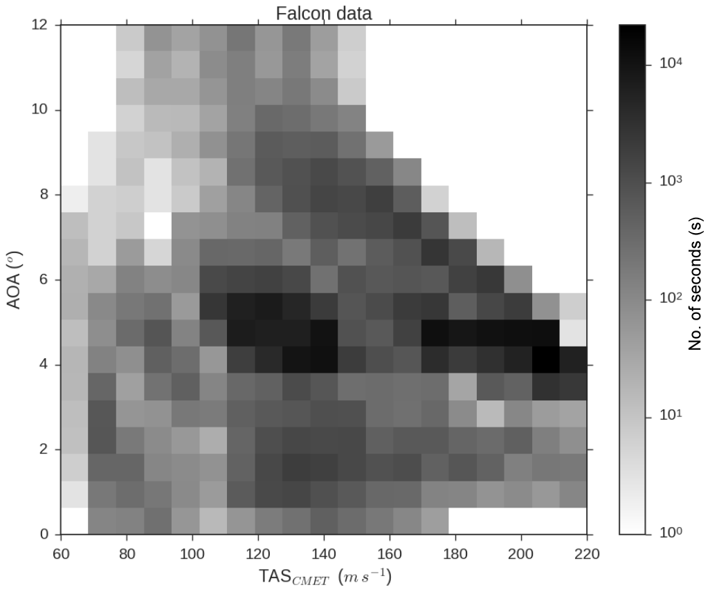
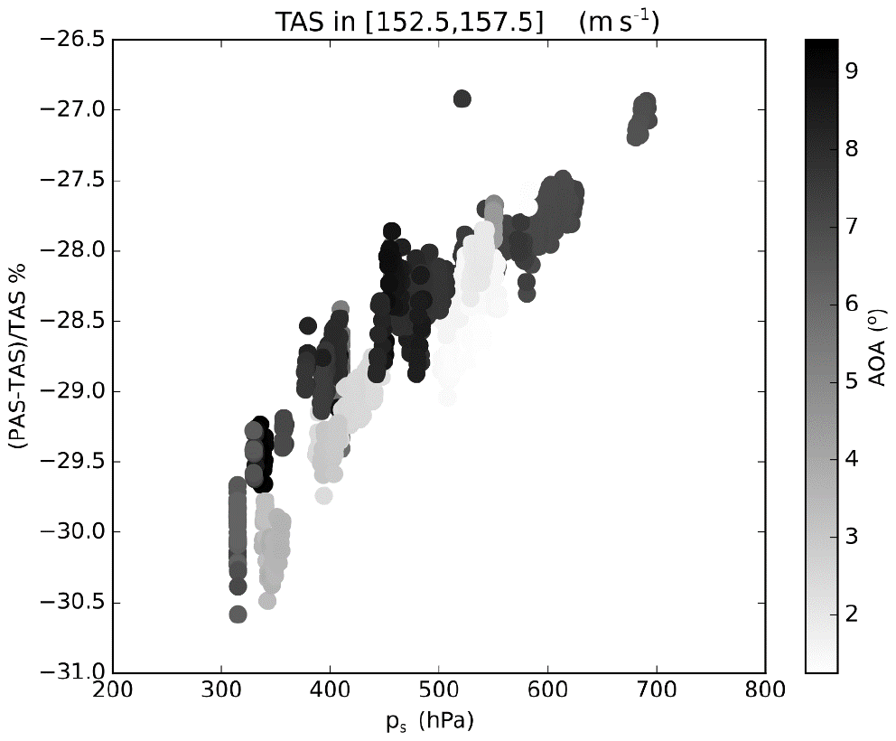
Figure A3 Deviation between PAS and TAS as a function of ambient pressure color coded with the AOA. Markers represent measurements at 1 Hz collected during the SALTRACE campaign covering an arbitrarily chosen TAS range from 152.5 to 157.5 m s⁻¹. A TAS range had to be chosen for this figure because the deviation between PAS and TAS depends also on TAS. However, also for other TAS ranges, the data show in a similar way that the AOA has only a minor impact on the measurements; i.e., (PAS–TAS)/TAS changes less than 2 % when the AOA changes.

Figure A4 Statistical analysis of differences between air speed in the free stream and at the probe during A-LIFE when CAPS was calibrated to match free stream conditions. TAS_CMET values were obtained by the CMET system and the PAS_CAPS was post-calculated using Eq. (1) and the dynamic and static pressure as well the temperature value at the probe obtained by inverting the relation described in Sect. 3.1.4. The histogram color map refers to the number of seconds of data at 1 Hz.

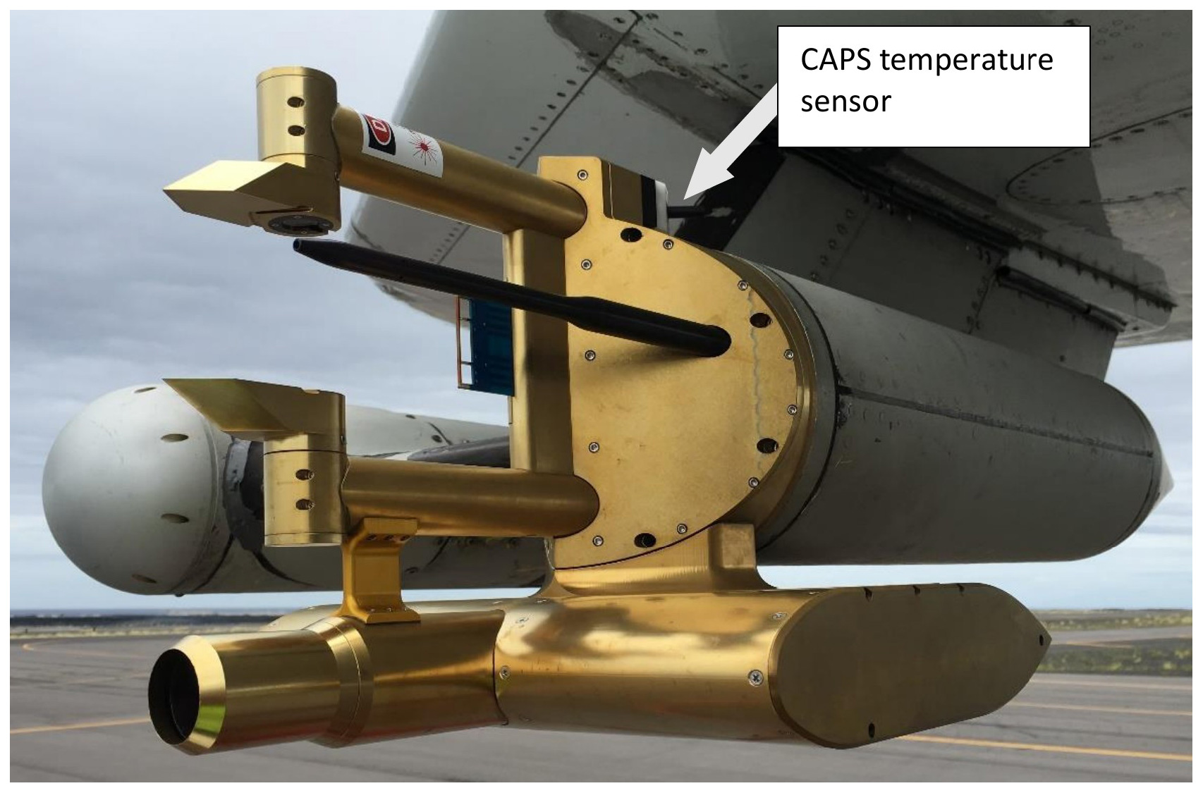
Figure A5 Photograph of the CAPS mounted at the wing of the NASA DC-8 research aircraft during ATom-4. The position of the temperature sensor is marked by the white arrow. (Photograph: Bernadett Weinzierl)

Table A1 Different speeds used.

Table A2 Abbreviations and symbols used.

Table A3 Sampling efficiency f_eff (%) for different test cases for different particle diameters d_p and densities ρ_p as shown in Fig. 8.