the Creative Commons Attribution 4.0 License.
the Creative Commons Attribution 4.0 License.
 | 29 Jun 2020
Low-level liquid cloud properties during ORACLES retrieved using airborne polarimetric measurements and a neural network algorithm
Daniel J. Miller
Michal Segal-Rozenhaimer
Kirk Knobelspiesse
Jens Redemann
Brian Cairns
Mikhail Alexandrov
Bastiaan van Diedenhoven
Andrzej Wasilewski
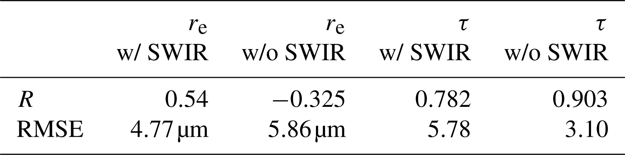
In this study we developed a neural network (NN) that can be used to retrieve cloud microphysical properties from multiangular and multispectral polarimetric remote sensing observations. This effort builds upon our previous work, which explored the sensitivity of neural network input, architecture, and other design requirements for this type of remote sensing problem. In particular this work introduces a framework for appropriately weighting total and polarized reflectances, which have vastly different magnitudes and measurement uncertainties. The NN is trained using an artificial training set and applied to research scanning polarimeter (RSP) data obtained during the ORACLES field campaign (ObseRvations of Aerosols above CLouds and their intEractionS). The polarimetric RSP observations are unique in that they observe the same cloud from a very large number of angles within a variety of spectral bands, resulting in a large dataset that can be explored rapidly with a NN approach. The usefulness of applying a NN to a dataset such as this one stems from the possibility of rapidly obtaining a retrieval that could be subsequently applied as a first guess for slower but more rigorous physical-based retrieval algorithms. This approach could be particularly advantageous for more complicated atmospheric retrievals – such as when an aerosol layer lies above clouds like in ORACLES. For RSP observations obtained during ORACLES 2016, comparisons between the NN and standard parametric polarimetric (PP) cloud retrieval give reasonable results for droplet effective radius (re: R=0.756, RMSE=1.74 µm) and cloud optical thickness (τ: R=0.950, RMSE=1.82). This level of statistical agreement is shown to be similar to comparisons between the two most well-established cloud retrievals, namely, the polarimetric and the bispectral total reflectance cloud retrievals. The NN retrievals from the ORACLES 2017 dataset result in retrievals of re (R=0.54, RMSE=4.77 µm) and τ (R=0.785, RMSE=5.61) that behave much more poorly. In particular we found that our NN retrieval approach does not perform well for thin (τ<3), inhomogeneous, or broken clouds. We also found that correction for above-cloud atmospheric absorption improved the NN retrievals moderately – but retrievals without this correction still behaved similarly to existing cloud retrievals with a slight systematic offset.
- Article
(4510 KB) - Full-text XML
- BibTeX
- EndNote


Advancing the scientific understanding of aerosol–cloud interactions is imperative for forming a more complete picture of the Earth climate system. These interactions are responsible for large uncertainties in our understanding of anthropogenic climate forcing (IPCC, 2013). The uncertainty primarily stems from the semidirect and indirect effects of aerosols on clouds (Wilcox, 2010, 2012; Lu et al., 2018), which have been found to have significant yet uncertain climate impacts (Sakaeda et al., 2011).
Not many other regions of the world have as consistent aerosol–cloud interactions as the marine boundary layer of the southeast (SE) Atlantic Ocean. This region is dominated by a semipermanent subtropical stratocumulus (Sc) deck that regularly interacts with significant biomass burning (BB) aerosols originating from natural and anthropogenic (agricultural) fires in central Africa during austral spring (July–October) (Zuidema et al., 2016). The aerosols are lofted into the mid-troposphere over land before being transported by large-scale circulation, eventually arriving above the marine stratocumulus deck (Adebiyi and Zuidema, 2016). This leads to near-persistent above-cloud aerosol (ACA) conditions that have consequential impacts on the radiative budget via direct radiative effects (i.e., enhanced aerosol absorption; Meyer et al., 2013; Zhang et al., 2016) and semidirect radiative effects that can induce numerous cloud adjustments (e.g., increased vertical stability, burn off, etc.; Koch and Del Genio, 2010; Wilcox, 2012). As a result of this unique environment, the SE Atlantic region has become the focus of sustained research efforts. In addition to orbital observations, several international field campaigns have overlapped with one another to explore this region, including CLARIFY (UK Met Office, CLoud-Aerosol-Radiation Interactions and Forcing: Year 2016; Zuidema et al., 2016), AEROCLO-SA (French National Research Agency, AErosol RadiatiOn and CLOuds in Southern Africa; Formenti et al., 2019), ONFIRE (US National Science Foundation, Observations of Fire's Impact on the Southeast Atlantic Region), LASIC (US Department of Energy, Layered Atlantic Smoke Interactions with Clouds; Zuidema et al., 2018), and ORACLES (NASA, ObseRvations of Aerosols above CLouds and their intEractionS; Zuidema et al., 2016). The last of these campaigns is the focus of this study.
To study this region, numerous state-of-the-art in situ and remote sensing instruments have participated in ORACLES flights in three deployments each austral spring from 2016 to 2018. As a consequence, the ORACLES dataset offers the opportunity to test and develop new remote sensing techniques – opening up the possibility of extending regional understanding to future satellite missions capable of making observations over global spatial scales and climactic timescales. One example is the upcoming NASA Plankton, Aerosol, Clouds, ocean Ecosystem (PACE) mission, which will deploy instruments with similar capabilities as the one we will focus on in this study (Werdell et al., 2019). From a passive cloud remote sensing perspective, the persistence of ACA in the ORACLES study region can represent a difficult and sometimes confounding issue. Cloud microphysical retrievals which do not consider the presence of the aerosol above the cloud can suffer biases due to the impact of absorption of the overlying BB aerosols in shortwave spectral bands. Most notably, this was found to be the case for the Moderate Resolution Imaging Spectroradiometer (MODIS) cloud retrieval product (Meyer et al., 2013). It is possible to correct for this impact, but an assumed aerosol model is required to constrain the otherwise unknown optical properties of the aerosol. On the other hand, there are some ACA retrieval methods that attempt to simultaneously retrieve full aerosol and cloud properties of ACA scenes. However, the existing techniques each still exhibit shortcomings when it comes to constraining aerosol absorption properties (e.g., single-scattering albedo or complex refractive index) and thus can result in an inaccurate representation of the direct radiative effect of ACA (Knobelspiesse et al., 2015; Yu and Zhang, 2013). One of the more promising approaches takes advantage of the large information content of multispectral, multiangular, and polarization observations. The vast information content of polarimetric observations provides ample opportunities to simultaneously retrieve aerosol and cloud properties. This methodology has been applied to both orbital (Waquet et al., 2009, 2013) and suborbital field campaign observations (Knobelspiesse et al., 2011b; Xu et al., 2018).
In this study, we make use of polarimetric observations obtained using the research scanning polarimeter (RSP) during ORACLES 2016 and 2017 field campaigns. The RSP is the airborne prototype for the aerosol polarimetry sensor (APS) built for the NASA Glory mission (Mishchenko et al., 2007; Peralta et al., 2007; Persh et al., 2010). While Glory did not successfully enter orbit due to a launch failure, the pair of RSP instruments, denoted RSP1 and RSP2, continue to make observations and have been deployed on over 25 field missions in the last 20 years. The instruments heritage, accuracy, and measurement characteristics make it well suited for observations of clouds (Alexandrov et al., 2012a, b; van Diedenhoven et al., 2016, 2013; Sinclair et al., 2017), aerosols (Chowdhary et al., 2001; Chowdhary and Cairns, 2002; Chowdhary et al., 2012; Knobelspiesse et al., 2011a, b; Wu et al., 2015, 2016; Stamnes et al., 2018), the ocean (Chowdhary et al., 2006, 2005b, a; Ottaviani et al., 2012), and snow (Ottaviani et al., 2015). In particular the cloud retrieval products of RSP are well established and validated (Alexandrov et al., 2015, 2016). In contrast, the retrieval of ACA properties has been implemented and tested only in a few case studies (Knobelspiesse et al., 2011b; Pistone et al., 2019).
The main limitation to the latter effort is the high computational expense, requiring numerous iterative calls to a time-consuming forward radiative transfer (RT) model. These iterative calls are made in an effort to match observations to a simulated scene, thereby retrieving optical and microphysical properties of the cloud and aerosol layers concurrently. Additionally, the dimensionality of the observational data (large for multiangle polarimetry) as well as the number of variables that are retrieved (large for ACA retrieval) can significantly slow down this type of approach. As a consequence of these computational limitations, accelerating these types of algorithms is critical to developing a useful retrieval product. Here, the neural network (NN) retrieval approach is useful, since it offers some important benefits and can be complementary to the solutions discussed above. First, it can be used to explore the nonlinear relationships between observation variables and retrieval properties in a manner that is independent of any imposed parameterized relationship between geophysical variables and the observations – providing unique insight into other inverse approaches. Second, after the network is trained, it is capable of transforming a vector of observed variables to retrievals rapidly by applying the “transfer function” resulting from the trained network. Third, the NN retrieval can serve as a prior state vector for an optimal estimation retrieval, accelerating and improving its results, as demonstrated by Di Noia et al. (2015) for a NN retrieval of aerosol properties using a multiangular and multiwavelength polarized ground-based instrument.
Here, we are capitalizing on our previous work in Segal-Rozenhaimer et al. (2018), where we have developed a NN retrieval scheme for low-level cloud properties. By focusing on clouds only, we can easily compare our results to the other RSP cloud retrieval algorithms to gain an understanding of how the NN retrieval is performing. Our original NN scheme was used twice: first as a base architecture for a sensitivity study and second as a retrieval scheme for low-level cloud properties during ORACLES 2016. The sensitivity study addressed numerous aspects in the algorithm design such as the type of input variables and their dimensionality, while the retrieval scheme used a preliminary (and somewhat limited) NN training set. Perhaps the most important outcome from this work was the determination of the type of input data required to use in a NN to retrieve cloud properties. For example, it is not necessarily obvious what pair of independent polarimetric observations would work best for a NN approach. We were able to demonstrate that the NN trained retrievals with the lowest root-mean-square error (RMSE) and highest correlation were found with inputs of the total reflectance (RI) and degree of linear polarization (DoLP) (Segal-Rozenhaimer et al., 2018). It is also worth emphasizing here that the existing passive cloud microphysical retrievals (e.g., bispectral; Nakajima and King, 1990; and polarimetric; Alexandrov et al., 2012a) either utilize observations of total or polarized reflectances separately to infer cloud droplet size distribution shape and cloud optical thickness. In contrast, this approach allows us to effectively mix the information contained in both total and polarized reflectance observations – resulting in a retrieval that attempts to be consistent for both observations. One major difference we are introducing in this work, compared to our previous NN, is the dimensionality of the input layer of the network. Previously, we used principal component analysis (PCA) to reduce the dimensionality of the input vector to improve the network in an attempt to increase convergence and generalization capability, as suggested in many prior studies (Di Noia et al., 2015; Del Frate and Schiavon, 1999; Del Frate et al., 2005; LeCun et al., 1989). This was performed separately on the RI and DoLP, which were then both used as an input to the NN. However, after training the network in this manner and applying it to a subset of ORACLES 2016 measurements, we found that the network placed more importance of RI than on DoLP measurements, despite the fact that the uncertainty of the latter is much lower (0.2 %) than the former (3 %). This resulted in poor accuracy and highly biased retrievals of cloud droplet size. In this work, we implemented a new approach to the network architecture that allows us to directly input the observation vector into the network – eliminating the need for dimensionality reduction and allowing us to treat disparate observational uncertainties in a more explicit manner.
The rest of the paper is organized in the following manner. Section 2 outlines the properties of the RSP instrument observations and uncertainties (Sect. 2.1) as well as specifics regarding the data obtained during the 2016 and 2017 ORACLES field campaigns (Sect. 2.2). Additionally, in that section we also give an overview of the various standard cloud property retrieval products from the RSP instrument, which we use to compare with our NN-based retrievals (Sect. 2.3). Section 3 focuses on new developments and improvements implemented in our approach to the NN retrieval scheme. Section 4 focuses on the output of the NN and the comparison of the NN retrievals to RSP's existing cloud retrievals during ORACLES 2016 (Sect. 4.2) and ORACLES 2017 (Sect. 4.3). Finally, in Sects. 5 and 6 we summarize our findings, discuss strengths and limitations, and indicate future goals of this research.
2.1 Research scanning polarimeter
The research scanning polarimeter is an airborne multiangular polarimetric instrument that continuously scans in the along-track direction, resulting in 152 views of each pixel at viewing zenith angles (VZA) up to (forward and aft of the flight direction). As a result, the RSP instrument has a very high angular resolution of . Measurements of the total and polarized reflectances are obtained at nine visible and shortwave infrared (SWIR) spectral channels with the following band centers: 0.410, 0.470, 0.555, 0.670, 0.865, 0.960, 1.59, 1.88, and 2.26, µm.1
Observed reflectances are defined in terms of the Stokes vector elements describing linearly polarized light (I, Q, and U) and are unitless due to normalization with respect to the incident solar irradiance in the following manner:
where RI is the total reflectance (including unpolarized and polarized light) and RQ and RU are the two perpendicular components of the linearly polarized reflectance. Additionally, r0 is the Earth–Sun distance in astronomical unit, F0 is the top-of-atmosphere solar irradiance, and θ0 is the solar zenith angle (SZA). It is important to note that the magnitudes of the linearly polarized reflectances (RQ, RU) are initially defined in an instrument polarization reference frame. In this work we transform from the instrument reference plane to the principal scattering plane (hereafter simply the principal plane), which is the plane containing both incident solar and observation viewing direction vectors. In the principal plane the singly scattered polarized reflectance of cloud droplets is fully described by RQ with measurements of RU expected to be near zero in magnitude (Mishchenko et al., 2007). However, for observations off of the principal plane the polarized reflectance is distributed between both RQ and RU. One way to separate the dependence on a geometric reference is to decompose the polarized reflectance measurements into the magnitude (independent of reference) and angle of the polarization vector (dependent on reference). For our purposes, the angle of the polarization vector is not particularly important, and the magnitude of the linearly polarized reflectance (RP) is the measurement of interest:
Additionally, it is also convenient to introduce the degree of linear polarization (DoLP), which is the ratio of the magnitude of polarized reflectance to the total reflectance:
The uncertainties in RI and DoLP differ from one another by an order of magnitude, with δRI≈3 % and δDoLP≈0.2 %, respectively. For RI, this measurement uncertainty is largely a result of radiometric calibration uncertainty. Because DoLP is a relative measurement, calibration uncertainty is less important, and sensitivity to random noise becomes the dominant source of uncertainty. A more complete description of RSP uncertainty and uncertainty models for the instruments can be found in Knobelspiesse et al. (2019).
As mentioned previously in Sect. 1, RSP2 flew throughout the ORACLES mission. In 2016, RSP2 was on board the NASA ER-2, but in 2017 and 2018 it was moved to the NASA P-3. It is worth noting that RSP1 was also deployed during the ORACLES 2016 campaign on board the P-3; however, there were data collection problems. Unexpected wind resistance at the instrument scanning assembly prevented it from spinning at the required rate, resulting in incomplete scans and poor georegistration. Successful data collection occurred for a small portion of the flights, but the limited nature of these observations did not justify application of the NN. RSP2 on the ER-2 had no significant issues throughout the 2016 campaign.
In practice, RSP is not oriented in the aircraft such that there is a symmetric range of VZAs about nadir viewing (i.e., 152 measurements spanning ). Rather, due to mounting constraints that result in aircraft vignetting, it is often positioned such that the range is : (forward to aft). For this reason, we restrict ourselves to a reduced range of angles that are symmetric about nadir (112 measurements spanning ). This restriction is important for our application, as it makes it possible to use the same NN for any heading.
RSP reflectances used in the NN dataset are aggregated to cloud-top height (CTH) following the same procedure as described in Fig. 1 of Alexandrov et al. (2012a).
2.2 Data from the ORACLES deployments
The datasets obtained during the first 2 years of ORACLES deployments in 2016 and 2017 differ from each other substantially. By design, each deployment of the ORACLES campaign was intended to target and characterize different months during the BB season (July through October), where the prevailing easterly wind transports the BB aerosols from sub-Saharan Africa fire events to the SE Atlantic, where the stratocumulus cloud deck is located (Swap, 1996; Costantino and Breon, 2013; Painemal et al., 2014; Zhang et al., 2016; Zuidema et al., 2016). To that end, the peak of the season (September) was the focus of the 2016 deployment, the beginning of the season (August) was the focus in 2017, and finally the end of the season (October) was the focus of the 2018 deployment. Additionally, from a logistical perspective, flight operations were not based out of the same location during each deployment. In 2016, flight operations were based out of Walvis Bay, Namibia (Fig. 1, dotted lines), and in 2017 (and also 2018) flight operations were moved north of the study region to the island of São Tomé (Fig. 1, dashed lines). The consequence of this logistical change is that there are regional differences in the cloud properties observed throughout the campaign. Walvis Bay is located close to the climatological center of the stratocumulus deck during the biomass burning season, whereas flights out of São Tomé in 2017 (and also in 2018) typically had to fly further south before encountering the stratocumulus cloud deck. As a consequence, from an environmental perspective, the clouds observed during the ORACLES 2016 field campaign were largely overcast marine stratocumulus but flights during 2017 observed less homogeneous marine boundary layer clouds associated with the transition between stratocumulus and broken cumulus cloud regimes. In addition to the regional differences, the behavior in the SE Atlantic changes to a greater extent seasonally and to a lesser extent interannually. Seasonally, the stratocumulus deck in this region shifts southward later in the season with the cloud fraction maximum occurring in September (Wood, 2012). In an interannual sense, the stratocumulus deck is modified by changes in lower tropospheric stability (LTS) that can be strongly correlated with sea surface temperature and free tropospheric temperature (Wood, 2012). Because the ORACLES campaign spanned multiple years and different seasons, the role of interannual variability is important to consider. However, for the purposes of this study, all of the variabilities result in greater diversity in the cloud retrieval dataset, which we can use to gain a better understanding of the behavior of our retrieval approach under a variety of cloudy conditions.
From an instrument perspective, the RSP flew on board different flight platforms during the 2016 and 2017 deployments. In 2016, the NASA high-altitude ER-2 was dedicated to remote sensing instruments, obtaining data from a near-consistent flight altitude above 18 km. On the other hand, during 2017 (and 2018) the RSP flew on board the NASA P-3 at a more variable range of altitudes, because the P-3 sampled throughout the boundary layer, in the cloud, in the aerosol layer, and above the cloud. As a consequence, the NN training sets for these 2 years differ from one another in order to be appropriately tailored to the airborne platform differences, mainly due to their different altitudes and the Rayleigh scattering differences. The training set for ORACLES 2016 was created for a constant aircraft altitude of 20 km, whereas the training set for ORACLES 2017 was constructed to account for level legs at different aircraft altitudes. The differences in the training set definition for each of these two datasets is further discussed in Sect. 3.1. Note that while ORACLES 2018 data are now available, they had not been available until after the analysis of the this NN implementation was complete. However, the 2018 NN results will also be available in our data archive when they are completed. (Refer to the Data availability section for a link to the data archive.)
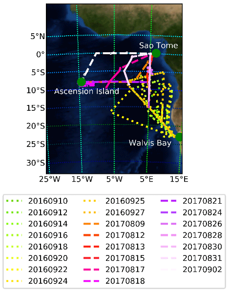
Figure 1Flight tracks and study regions for the ORACLES 2016 (dotted lines) and 2017 (dashed lines) field campaigns. Additionally, key take-off and landing locations are indicated and labeled with green circles. Map data based on the Blue Marble: Next Generation from the NASA Earth Observatory.
As with any field campaign, instrument-specific complications arose that need to be considered. For example, the SWIR detectors of RSP must be cooled to obtain SWIR reflectances without significant noise; however, during the 2017 field campaign there was a lack of liquid nitrogen to cool the detectors during some of the flights. As a consequence, much of the 2017 dataset lacks data from the SWIR channels. To explore the consequence of the loss of the SWIR channels on our retrievals, we created two different training datasets for our ORACLES 2017 NN retrieval scheme: one excluding the SWIR channels (applied on the entire dataset) and one that included the SWIR channels during training (applied on the flights that acquired data with these channels).
Before performing the comparison of different retrieval methods, presented in Sect. 4, RSP data are first screened for a number of conditions to obtain useful comparable retrieval datasets. The philosophy behind this screening process is to obtain the best data for usage in this study but at the same time not cast aside NN retrievals that may be useful in future studies. In addition to RSP data, we also use cloud-top height data from the NASA Langley airborne second-generation high spectral resolution lidar (HSRL-2) to remove observations of high-level or multilayer clouds in an attempt to limit the retrieval to low-level marine boundary layer clouds (Hair et al., 2008; Burton et al., 2018). To that end, the following screening criteria are applied to the datasets compared:
-
cloudy scenes as identified by other RSP retrieval methods,
-
successful RSP retrievals using all other techniques,
-
coincident RSP and HSRL-2 data for cloud-top height definition, and
-
instances with HSRL-2 cloud-top height below 2 km.
In a few limited cases coincident HSRL-2 and RSP data were not available, which precludes some retrieval data from the screening criteria above. The HSRL-2 screening criteria were removed in the final data product (refer to the Data availability section) so that it could include NN retrievals for the entire RSP dataset. Also included with the dataset is a guide discussing how to evaluate the screening flags and select data suitable for other uses.
2.3 Standard RSP cloud retrievals
The shortwave radiative impact of clouds largely depends on microphysical-scale cloud properties that define the droplet size distribution (DSD) (Twomey, 1977). Additionally, the DSD also plays an important role in cloud-precipitation processes (Pruppacher and Klett, 1978). In cloud remote sensing it is common to describe the cloud droplet size distribution using the gamma distribution presented in Hansen and Travis (1974), because it is both mathematically convenient and fits well to in situ observations (Deirmendjian, 1964; Tampieri and Tomasi, 1976):
This is a three-parameter distribution characterized by a droplet number concentration (N0, cm−3), a droplet effective radius (re, µm), and a droplet effective variance (ve, −). The normalization constant for this distribution, C, is calculated based on these parameters and the gamma function (Γ). The effective radius is a cross-section weighted droplet size that, for the purposes of light scattering applications, is usefully related to the scattering droplet size described in Hansen and Travis (1974). The effective variance is related to the droplet size distribution dispersion and can also be interpreted as a measure of the asymmetry of the droplet size distribution.
The existing RSP liquid cloud retrieval products include three very different methods of inferring cloud microphysical information. Each of these methods differs from one another in fundamental ways that include integrating observational data of different types (i.e., total or polarized reflected light), capability of retrieving different combinations of variables (i.e., some combination of re, ve, and τ), and sensitivities (i.e., to cloud vertical profile, aerosol above cloud, or microphysical regime).
The first method, often referred to as the bispectral Nakajima–King (NJK) method, is an approach that takes advantage of a difference in sensitivity to cloud optical thickness and effective radius in a pair of spectral total reflectance bands (Nakajima and King, 1990). One band is in a scattering-dominated visible-to-near-infrared (VNIR) band, while the other is in a more absorptive shortwave infrared (SWIR) band. The NJK retrieval performed by RSP makes use of nadir-viewing total reflectances in the 0.865 µm and the 2.26 µm or 1.59 µm spectral bands. For the purposes of this study, we focus on the RSP NJK retrieval using the 0.865 and 2.26 µm spectral band combination. This retrieval, most notably implemented for the MODIS cloud retrieval product, is typically performed as a two-dimensional interpolation of observed reflectances within a discrete look-up table (LUT), relating reflectances to unique pairs of re and τ values (Platnick et al., 2016). This particular method is also important because it obtains a retrieval of cloud optical thickness, while the following two methods, which are based on polarized reflectances, retrieve only droplet size distribution information (re, and ve). As a consequence, these other methods secondarily perform an optical thickness retrieval in a manner similar to the NJK retrieval but with a single VNIR band LUT with a preconstrained re obtained via a polarimetric retrieval. In the context of the ORACLES field campaign it is also important to emphasize that the NJK method has been shown to be systematically biased by the presence of ACA – resulting in a high bias in both re and τ retrievals that is highly dependent on aerosol model assumptions, especially those that can impact absorption (e.g., aerosol single-scattering albedo or refractive index) (Meyer et al., 2013).
The second RSP retrieval, referred to here as the parametric polarimetric method (PP), makes use of a library of calculations that describe the angular distribution of single-scattered polarized light (known as polarized phase functions −P12). The phase functions and reflectances are both characterized by angular rainbow features (appearing between scattering angles of 130 and 170∘) that predictably shift and erode depending on the properties of the particular droplet size distribution (i.e., the re and ve pair) (Bréon and Goloub, 1998). Because polarized reflectances are dominated by single scattering, this library can be used to obtain a best fit solution that matches the observed multiangular RP or DoLP in a single spectral band. The phase function is then modified by parametric functions that account for Rayleigh scattering and multiple scattering effects. The best fit solution of this parametric phase function to the observed multiangular reflectance corresponds to the droplet size distribution parameters retrieved (Alexandrov et al., 2012a). The PP retrieval can be performed for a number of different spectral bands, however, in this study we make use of the retrieval performed for the 0.865 µm band. This is because the longer shortwave spectral bands have been shown to be more sensitive to a greater range of droplet sizes at a fixed angular resolution (Miller et al., 2018).
The third RSP retrieval method is a non-parametric approach, known as the rainbow Fourier transform (RFT), that retrieves the droplet size distribution in a functional form via a mathematical transformation mapping the polarized reflectance in angular space to the droplet size distribution in microphysical space. As the name indicates, this approach is similar to the relationship between oscillatory signals (frequency space) and their corresponding Fourier transforms (amplitude space) (Alexandrov et al., 2012b). This method is useful for evaluating the assumption that droplet size distributions are well behaved and mono-modal – an implicit assumption for both of the gamma-distribution parameter retrievals discussed previously (Alexandrov et al., 2016). The RFT retrieval reports the distribution shape, but it also reports the best-fit gamma-distribution parameters of the two most prominent modes of the size distribution, resulting in re and ve retrievals for each mode. When we discuss the RFT retrieval in this study as a single re or ve value, we are always referring to the most prominent mode of the size distribution.
The physical differences between NJK and PP cloud property retrievals was recently the topic of research in Miller et al. (2018). One of the findings of that study was that high spatial resolution retrievals (50 m) mostly agreed with one another to within the measurement uncertainties of the two methods. However, at coarse spatial resolutions (>300 m) observations of spatially inhomogeneous cloud fields caused the NJK retrieval to be biased high, resulting in differences between the two retrieval approaches. In the context of this study, airborne observations made by RSP have quite a high spatial resolution (on the order of tens of meters to hundreds of meters, depending on aircraft altitude), which should avoid some spatial inhomogeneity issues in this comparison. Another finding by Miller et al. (2018) was that there can be significant high biases for the NJK retrieval when droplet sizes become small (re≈5 µm) or for optically thin clouds (τ<3). Given the high spatial and angular resolution of the RSP retrievals in this study, it is likely that biases associated with the “small and thin” population will be the most prevalent source of bias in our data.
In this study we intend to make informed comparisons between these already existing retrievals and the NN retrieval. However, before doing that it is important to evaluate how these disparate retrieval products compare to one another. To that end, Fig. 2 evaluates each of the retrievals against one another in much the same manner as in Miller et al. (2018). All of these comparisons are made using ORACLES data that have been previously screened for multilayer clouds, as detailed in Sect. 2.2. The comparison of NJK and PP retrievals of re are shown as density regressions for the ORACLES 2016 (Fig. 2a) and ORACLES 2017 (Fig. 2d) datasets. From the ORACLES 2016 comparison, it is evident that the two retrievals are similar to one another – with a correlation of R=0.747, a mean bias of −0.830 µm, and a RMSE=1.74 µm. It is noteworthy that despite being similar overall, the RMSE of the retrieval comparison is actually still quite large with Fig. 2b, indicating that the re retrieval bias is being driven by retrievals of the low τ population (τ<3). With that in mind, the statistics for comparisons of the two retrievals excluding the low τ population are significantly improved. The comparison for ORACLES 2017 is more complicated, with increased relative occurrence of thin clouds and increased spatial inhomogeneity, the statistical metrics are much poorer – with a correlation of R=0.201, a mean bias of −1.41 µm, and a RMSE=3.38 µm. However, this behavior is still, to a large extent, associated with the low τ population with statistics improving when that population is excluded (looking only at τ>3) as indicated in Fig. 2. For both ORACLES 2016 (Fig. 2c) and ORACLES 2017 (Fig. 2f) datasets, the comparison of τ reveals that there is typically very little relative bias. In some cases, there are biases observed between the two retrievals corresponding to small NJK re retrievals – indicating that using the PP constrained re retrieval produced a different τ retrieval. Given the statistical properties of the comparisons of these two well-established retrieval approaches, we should expect to be satisfied if we find a similar degree of agreement between the NN retrieval and any of the standard RSP retrievals.
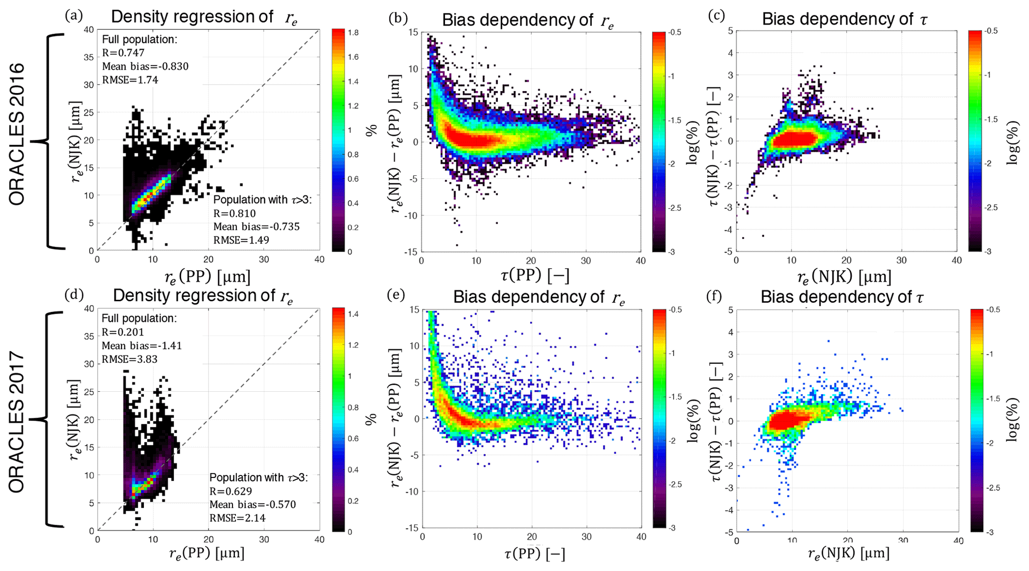
Figure 2A series of comparisons between the PP (using the 0.865 µm polarized reflectances) and NJK retrievals (using the 2.26 µm SWIR band) made by RSP during ORACLES 2016 (a–c) and 2017 (d–f). In panels (a, d) NJK re (y axis) and PP re (x axis) retrievals are compared using a density regression plot with a color bar that indicates the percentage of observations contained in each bin and a dashed one-to-one line. In panels (a, b) the correlation, mean bias, and RMSE are reported for the full retrieval population, while the same statistics are also reported for thick clouds (τ>3) only in (c). Panels (d–f) use a different color bar that emphasizes features of smaller populations using the logarithm of the percentage of observations in each bin. In panels (b, e) we display the bias between NJK and PP retrieval of re (y axis) is shown with respect to the PP retrieval of τ (x axis). Finally, in panels (c, f) the bias between NJK and PP retrievals of τ (y axis) is shown with respect to the NJK re retrieval.
As discussed in Sect. 1, the NN architecture implemented in this study has changed significantly in response to the findings of our previous work (Segal-Rozenhaimer et al., 2018). In Sect. 3.1 we will discuss the definition of the training set and particularities to the first 2 years of the ORACLES field campaign. Then, Sect. 3.2 discusses our new approach to preprocessing input observations and uncertainties of total and polarized reflectances. Finally, in Sect. 3.3 we outline the architectural variables such as network structure, learning rate, etc.
3.1 Training set simulations
The synthetic observational dataset used to train the NN is created using a vectorized radiative transfer (RT) model to generate total and polarized reflectances that mimic the conditions of the observations made by the RSP instrument during the ORACLES field campaign. The RT model used in this study is the plane-parallel (1-D) polarized doubling–adding (PDA) model developed at the NASA Goddard Institute for Space Studies. This model is built upon the methods described in van de Hulst and Irvine (1963) and can efficiently solve radiative transfer problems in optically thick atmospheres (Hovenier, 1971; Hansen, 1971; Hansen and Travis, 1974; De Haan et al., 1987). This PDA radiative transfer code was also selected to be used for inversions during the Glory mission and therefore was specifically improved and tailored for polarimetric accuracy (Cairns and Chowdhary, 2003). As a consequence, it is very efficient at generating the simulated multispectral, multiangular polarimetric observations required to mimic the observations of the RSP instrument.
The training sets for the operational NN were generated based on the range of cloud properties observed in ORACLES 2016 (from RSP and in situ cloud measurements) and were tailored for each of the airborne platforms, as discussed in Sect. 2.2. Compared to our training set generated in the Segal-Rozenhaimer et al. (2018) study, these training sets expand the relative azimuth angle (RAA) range significantly (from to ) as shown in Table 1. This new RAA range covers all possible azimuth geometries, since radiative transfer is symmetric about the solar plane and because the RSP scans in both forward and aft directions.
For all training sets, cloud-top height was fixed at 1 km, which was found to be a reasonable assumption based on other independent measurements during the ORACLES campaigns. Also, since the ER-2 is a high-altitude platform that flies at a constant altitude, the training set simulations (Table 1) were made for a constant aircraft altitude of 20 km. However, since the P-3 is a low-altitude flying platform, altitude variations were much larger than the ER-2, and the training set was constructed to predict measurements obtained along constant level legs of various altitudes (Table 2). Additionally, there was slightly more variability in cloud-top height during 2017 as the clouds observed were often transitioning between low-level stratocumulus regime into mid-level cloud regimes. Since the atmospheric scattering between the flying platform and the cloud top has an effect on the measured signals, the generated cases might not be optimal for all the scenes flown during 2017. This is a relatively simplistic approach and certainly does not capture the full variability of the observed data; as a result, the training set simplifies some aspects of nature. For example, this approach would neglect the Rayleigh shielding effect, where an increased cloud-top height would exclude more of the lower atmosphere and therefore it's contribution to the Rayleigh scattering signal from observed reflectances.
Compared to the predecessor paper Segal-Rozenhaimer et al. (2018), we used a larger set of geometries and wider range of parameter values but many of the same approximations. For example, this training set assumes plane-parallel radiative transfer (neglecting 3-D radiative effects) and a “black” ocean surface with no reflections due to sun glint or ocean color. The former is beyond our computing resources and desired level of parameterization, while the impact of the latter is expected to be heavily attenuated by the cloud. It should also be noted that, as a matter of practice, we attempted to keep the size of the training set used in this study reasonable to leave open the possibility of massively expanding the training data to include a large number of other independent variables describing above-cloud aerosol properties for use in future projects. The consequences and limitations of using this limited training dataset and the role that other training set decisions play in the behavior of our retrieval results will be discussed in Sects. 4 and 5.
Table 1Parameter grid space used to generate the training set for the operational NN used for cloud retrievals from the ER-2 during the ORACLES 2016 field campaign. This contains N=44 064 feature vectors, with each vector containing N≈1600 labeled datapoints corresponding to radiometric variables (I and DoLP), wavelengths, across all VZAs. Aircraft altitude is set as constant at 20 km, and cloud top altitude was also fixed at 1 km.
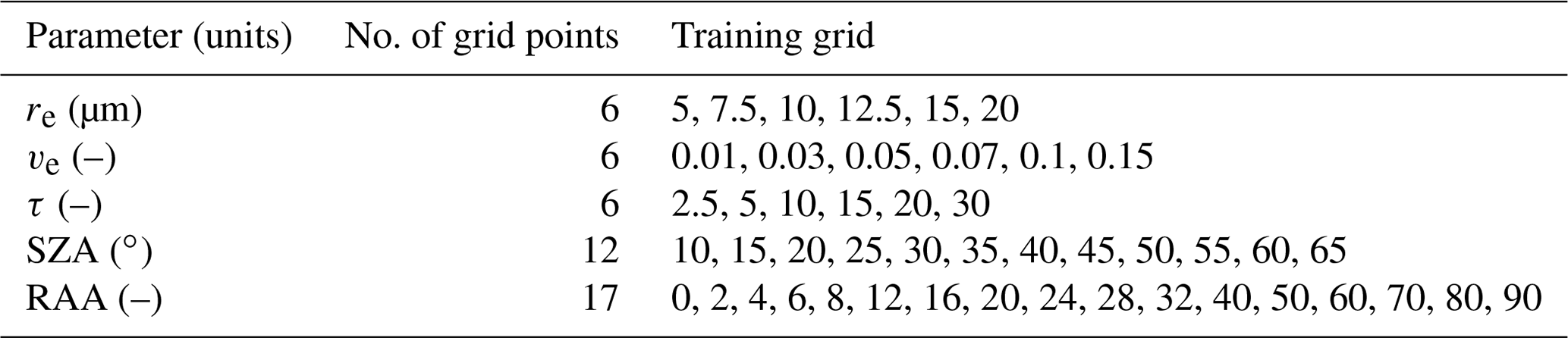
Table 2Parameter grid space used to generate the training set for the operational NN used for cloud retrievals from the P-3 during the ORACLES 2017 field campaign. This contains N=261 144 feature vectors, with each vector containing N≈1600 labeled datapoints corresponding to radiometric variables (I and DoLP), wavelengths, across all VZAs.

3.2 Preprocessing input observations
In our former NN retrieval scheme, we reduced the dimensionality of the input layer by reducing measurement vector inputs to principal components (PCs) before introducing them as input to the NN (Segal-Rozenhaimer et al., 2018). Our improved retrieval scheme described here is instead trained with and applied to the measurement vector itself. This solution was conceived to allow for more appropriate weighting of RI or DoLP, which have significantly different measurement uncertainties. The size of the input layer changed from 122 inputs (100 PC for DoLP, 20 for RI, and the two geometry inputs, i.e., SZA and RAA for each case) to 1570 (concatenating RI and DoLP, each spanning 784 values, covering the 112 instrument viewing angles in seven wavelengths plus the two geometry input values). To accommodate this 10-fold increase in the size of the input layer, we implemented a new approach to our NN architecture, which will be discussed in Sect. 3.3. The advantage of this approach is that it allows us to adequately scale (weight) the different input sources (RI and DoLP) according to their measurement uncertainty. This is specifically important for polarimetric observations, because both the magnitude and uncertainty of RSP observations of RI and DoLP differ by an order of magnitude. The uncertainty in RI is δRI≈3 % and is largely dominated by systematic calibration-dependent biases, whereas the uncertainty in DoLP is δDoLP≈0.2 % and is largely dominated by random noise that varies with scene reflectance (RI). Without consideration of the relative magnitude and uncertainty, a NN incorporating both of these types of observations would erroneously rely too much on high-magnitude and uncertainty RI observations at the expense of low-magnitude and uncertainty DoLP. To avoid this issue, we incorporate knowledge of measurement uncertainty into a vector standardization process that is applied prior to NN training and application. Typically, standardization scales the input state vector by the variability in the dataset such that all inputs are constrained within a range in the following manner,
where is the mean of all x over all elements i, and s is the associated standard deviation. In contrast to this, we have modified this process so that measurement uncertainty is incorporated into the standardized data, such that the standard deviation is replaced by the expected measurement uncertainty of the mean observation obtained for the same geometry and band ,
where the measurement uncertainty, σ, is calculated using the RSP uncertainty model in Knobelspiesse et al. (2019). We have explicitly noted the dimensions over which the average is calculated (solar zenith angle, view zenith angle, relative solar-view azimuth angle, spectral band [θ0, θ, Δϕ, λ]), such that a new standardization is calculated for the population of all training set data with the same geometry and wavelength. Both the training set and the observations go through this preprocessing standardization process. After this standardization relative to instrument uncertainty, the range of variability in the DoLP training set input was approximately 4 times greater than the range of variability in the RI. As a result the network initially places greater weight on changes in DoLP than on changes in RI. It is also important to note here that after this initial preprocessing step, we also perform further input regularization and normalization as described in the following section to help the network converge quickly during training.
3.3 Neural network architecture and training
To handle the order-of-magnitude increase in the new input layer, we have been pushed to develop a deeper network architecture. The new network, shown in Fig. 3, consists of four subsequent hidden layers, each with 1024 nodes. This deep architecture contains more parameters that need to be trained, and as a consequence our approach to training has also changed. In our previous work, we used a pure stochastic back-propagation method that updated the weights in the hidden layer after each training sample. This network is instead trained using a mini-batch method, where a batch of samples (128) is presented to the network and the hidden layer weights are only updated after each batch has been processed. In this architecture, following each hidden layer, there is a batch normalization (BN) layer applied to the outputs of the layer. The purpose of the BN layer is to increase the stability of the neural network, by subtracting the batch mean and dividing by the batch standard deviation. By applying this transformation, it keeps the inputs into the subsequent activation layer stable (not too high and not too low), maintaining the mean activation close to 0 and the activation standard deviation close to 1, to help with the network training convergence. In the activation layer, we make use of either a hyperbolic tangent (tanh (θ)) or rectified linear unit function (ReLU(θ)), the latter of which is zero for all negative inputs and linearly increases for positive inputs. The tanh activation is widely used as the standard in NN literature (e.g., LeCun et al., 1989, 1998), while ReLU is gaining more popularity recently due to its simplicity and its ability to greatly accelerate the convergence of stochastic gradient descent (SGD) algorithms and their variations (Krizhevsky et al., 2012). In Segal-Rozenhaimer et al. (2018), we did not notice a large difference between these two activation functions, but for this larger NN, we find differences in retrieval performance that we will discuss in detail in Sect. 4. Finally, the output layer activation function is linear, with a loss function defined as the mean-square error (MSE) and results in the predicted values of τ, re, and ve.
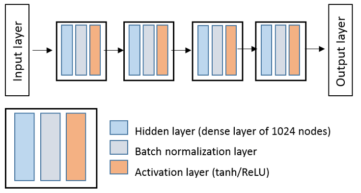
Figure 3Architecture of the operational NN scheme used for the retrieval of ORACLES 2016–2017 RSP measurements. The network contains four subsequent hidden layers, as detailed in the text.
During the training process, the input vector, which has already been preprocessed as detailed in the former section, is further linearly scaled to have values between −1 and 1. This is performed to allow for better convergence during training. Also, the training process is being regularized by adding Gaussian noise to the input layer during the training phase. The optimization algorithm used here is Adam (Adaptive moment estimation), implemented within the Keras python API (Chollet, 2017) with a TensorFlow back end (a system for large-scale machine learning) (Abadi et al., 2016). In comparison with the classic stochastic gradient descent (SGD) optimization algorithm, Adam is computationally efficient, has little memory requirements, and is well suited for problems that are large in terms of data and/or parameters (Kingma and Ba, 2014). The network is trained with a learning rate of 0.0001 using the “mini-batch” method to complete an epoch, while the number of epochs per training scenario was 100. Following training, the network was evaluated using an evaluation dataset consisting of a subset of training set data that were set aside during the training phase. Taking the network trained for ORACLES 2016 using tanh activation as an example, comparison with the evaluation dataset resulted in correlations of 0.999, 0.987, and 0.941; absolute biases of 0.016, 0.044 µm, and 0.094; and RMSEs of 0.021, 0.076 µm, and 0.16 each for τ, re, and ve, respectively. The results for τ and re are quite promising, but the RMSE in the ve evaluation after training is enough to span the possible state space – an indication that this network cannot adequately retrieve ve. It is important to note that other neural network studies have demonstrated better retrieval quality for ve with different input and architecture decisions (Di Noia et al., 2019). We also compared ve(NN) to RSP retrievals and found significant variability and large biases that were inconsistent with both studies of RSP retrieval sensitivity (Alexandrov et al., 2012a), as well as other studies focused on similar polarimeter retrievals (Shang et al., 2019).
4.1 Initial output and postprocessing
The output from the network initially reveals some issues that still need to be addressed. Our approach to evaluating the behavior of the output layer results is to explore comparisons to the RSP retrievals. Throughout the following we will refer to network output layer results as the “initial output” to indicate that it has not undergone any postprocessing. As indicated in Sect. 2.3, we are particularly interested in the RSP PP retrieval comparison as this provides the most consistent retrieval results in conditions with varying cloud inhomogeneity and in the presence of above-cloud aerosols. Overall, this comparison revealed correlations for the re retrievals are lower (R≈0.7) than for the τ (R≈0.9) retrieval irrespective of the network activation function used. An interesting finding of this initial analysis was that networks using different activation functions produced different behaviors for the retrievals of τ than they did for re. This is demonstrated in Table 3 using the ORACLES 2016 network and data, where the correlations for re retrievals improve for networks using a tanh activation function, while in contrast τ retrievals have improved correlations for networks using a ReLU activation function. This behavior is a symptom of a feature we observed rather than being linearly related to the PP retrieval of τ; the tanh-based τ retrieval demonstrated a nonlinear or logarithmic dependence with increasing τ. A similar behavior was exhibited for the PP retrieval of re and the ReLU-based re retrieval. As a consequence, throughout the rest of this study, we will perform retrievals for re and τ with two different networks: for re we make use of the tanh network and for τ we make use of the ReLU network. This approach will be further discussed in Sect. 4.2.
Table 3Correlations between existing RSP retrieval of re and τ with raw NN retrieval output with different activation functions (ReLU(θ) vs. tanh (θ)). Note that the p values for all of these comparisons are much less than 0.05.

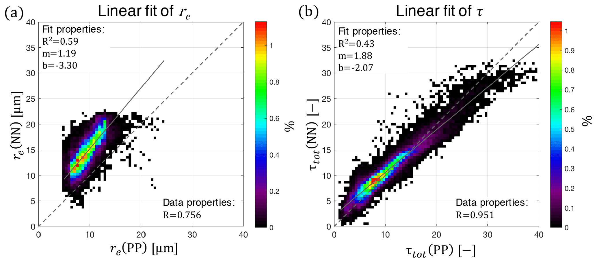
Figure 4Density regression plots demonstrating behavior of raw NN retrieval output for re (tanh network, a) and τ (ReLU network, b). The dashed gray line in each plot indicate the 1:1 line, while the solid gray line indicates the linear best fit line for the dataset.
Beyond simply evaluating correlations, the raw output of the network exhibits clear linear offsets when compared to the other RSP retrievals. In particular we emphasize this behavior for the PP retrievals in Fig. 4. This linear bias was absent during our training set validation exercise in Sect. 3.3, implying that this systematic offset is a consequence of differences between training set and observational data. Despite this linear bias, the high correlations of these retrievals imply that the NN retrieval is otherwise generally performing correctly. In particular, we expect that this bias is an expression of a difference between the assumptions built into the network training dataset that differ from the observation dataset. We will discuss the possible sources of these differences in Sect. 5.
Given the high correlations, linearity of the initial output, and results from the network training evaluation, we believe the linear offsets of these regressions are artifacts. To correct the persistent linear offset of the NN retrievals, we apply a linear scaling to them by creating what we refer to as our adjusted NN retrieval product. Ideally and in principle this could be done with a small validation dataset that is not related to the retrieval products we hope to later compare our results to. Without an external dataset to scale to, we have decided to linearly scale the NN retrievals to a subset of 10 % of the total population of RSP data (in this example for the ORACLES 2016 dataset). This avoids explicitly fitting all NN retrievals via fitting. This dataset is then regressed against the corresponding τ(PP) and re(PP) retrievals to obtain two linear correction terms, the offset bias (b) and the scaling bias (m),
where corresponds to a linearly adjusted neural network retrieval output, m is the scale correction, and b is the linear offset correction. After the components of this linear adjustment are determined using the subset of PP retrievals, the NN retrievals are adjusted (i.e., the product is created). Finally, this adjusted NN retrieval product can be compared to the other retrievals using the full RSP dataset – including the portion that was excluded from this correction definition exercise. The application of this linear correction does not influence the correlation of the retrievals; however, it does result in lower mean and RMSE biases for this ORACLES 2016 example shown in Fig. 4. For re, the mean bias is reduced to 0.023 µm and the RMSE is 1.74 µm, whereas for τ the mean bias is −0.050 and the RMSE is 1.82. Further discussions of the behavior of the adjusted NN datasets are separated into Sect. 4.2 and 4.3, where each discusses and highlights behaviors of the NN retrieval for the ORACLES 2016 and 2017 datasets, respectively.
4.2 Results for ORACLES 2016
From a number of perspectives, the ORACLES 2016 campaign data are easy to work with: RSP was flying on a dedicated remote sensing platform (NASA high-altitude ER-2), there were prevalent observations of clouds, and data availability was often not an issue. As a consequence, the dataset analyzed here is large – including 6 d of flights with N=72 542 retrievals that pass all of the analysis filter criteria introduced in Sect. 2.2.
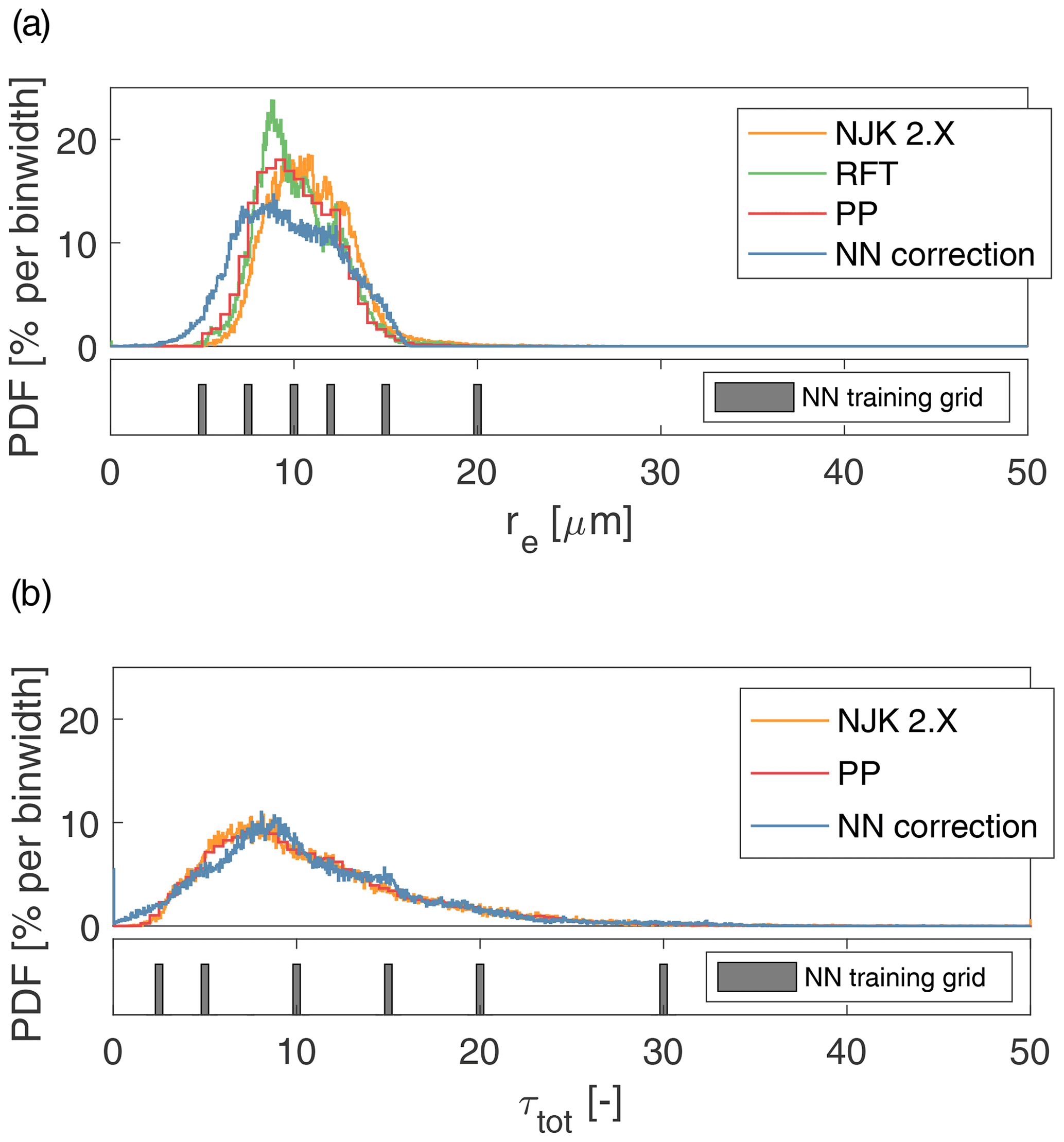
The overall statistics of retrievals during ORACLES 2016 highlight features and challenges for the development of the NN retrieval. At first glance, the retrieval probability distribution functions (PDFs, % per bin unit) in Fig. 5 reveal that all of the RSP cloud retrievals are similar to one another – with droplet sizes that are small (), optical thicknesses are largely moderate (), and relatively few occurrences of thicker clouds (τ>30). The standard RSP cloud retrievals exhibit some similar differences and behaviors to those highlighted in Sect. 2.3, specifically that the NJK retrieval is shifted toward larger droplet sizes than the other two methods. An evident feature of the NN retrieval PDF is that there is some clustering occurring near discrete values associated with the training set grid (shown below each PDF as defined in Table 1), as demonstrated by the NN training grid bins shown below each PDF. This effect is particularly evident in the τ histogram where peaks in the PDF appear near training set grid points (allowing for some shifting associated with the postprocessing correction). The overall shape of the NN retrieval distributions resemble that of the other RSP retrievals, although the NN retrievals of re appear to be slightly more broadly distributed.
A closer examination of the comparison of NN retrievals and the PP retrievals is required to reveal if the NN retrieval exhibits any systematic dependence on different retrieval populations. This is accomplished using the joint density regression of the NN retrievals against each of the PP retrievals shown in Fig. 6. Comparisons of the NN retrievals to the RSP PP retrievals reveal mean biases for re and τ of 0.023 µm and −0.050, respectively, with RMSEs for re and τ of 1.74 µm and 1.82, respectively. In the case of the re retrieval, the NN retrieval appears to miss the large re(PP) retrieval population above 15 µm, and there is much more variability in small re(NN) retrievals in part because there are no re(PP) retrievals below 5 µm. Whether or not such small re(NN) results are reasonable remains an open question as this regime is often excluded from look-up table datasets, whether for sensitivity reasons (NJK has multiple solution issues) or simply because they are not expected to be common.
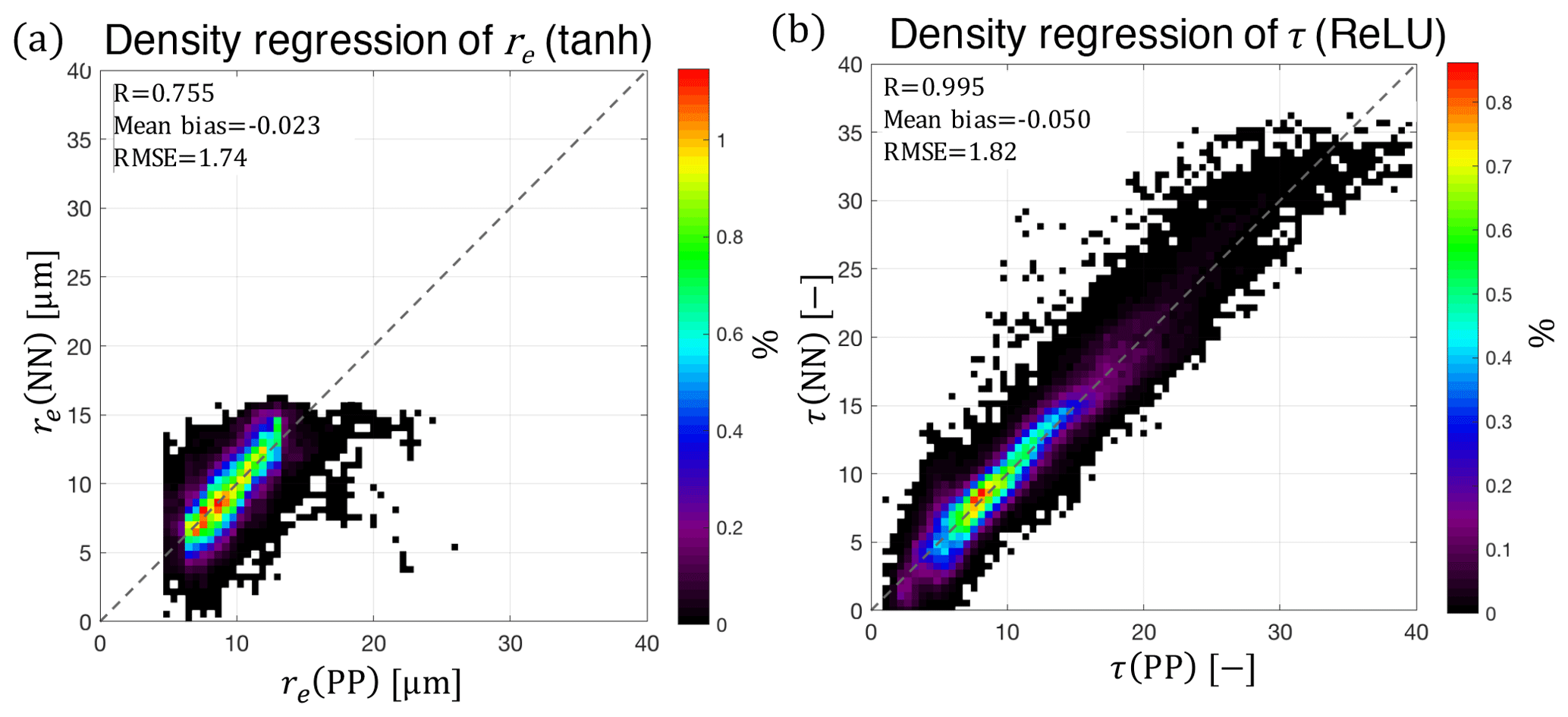
Figure 6Density regression plots comparing all of the ORACLES 2016 NN retrievals (y axis) and PP retrievals (x axis) of re (a) and τ (b). The density of the joint histogram is shown in a linear scale indicating the percentage of the retrieval population within each bin. A dashed line is also plotted indicating the 1:1 line.
A flight track time series is useful for emphasizing how the observed spatial variability of the NN retrieval behaves relative to the other retrieval products. The example flight track time series in Fig. 7 reveals that there is clearly good match-up between cloud optical thickness and effective radius retrievals. The statistics of this time series show improvement relative to our previous study. In particular the new NN exhibits a retrieval of re that is significantly improved relative to Segal-Rozenhaimer et al. (2018) – with correlations between re(NN) and re(PP) of 0.587 and an RMSE between re(NN) and re(PP) of 1.74 µm . The new network performs just as well on the τ retrieval as our previous study – with correlations τ(NN) and τ(PP) at 0.951 and an RMSE between τ(NN) and τ(PP) of 1.842.
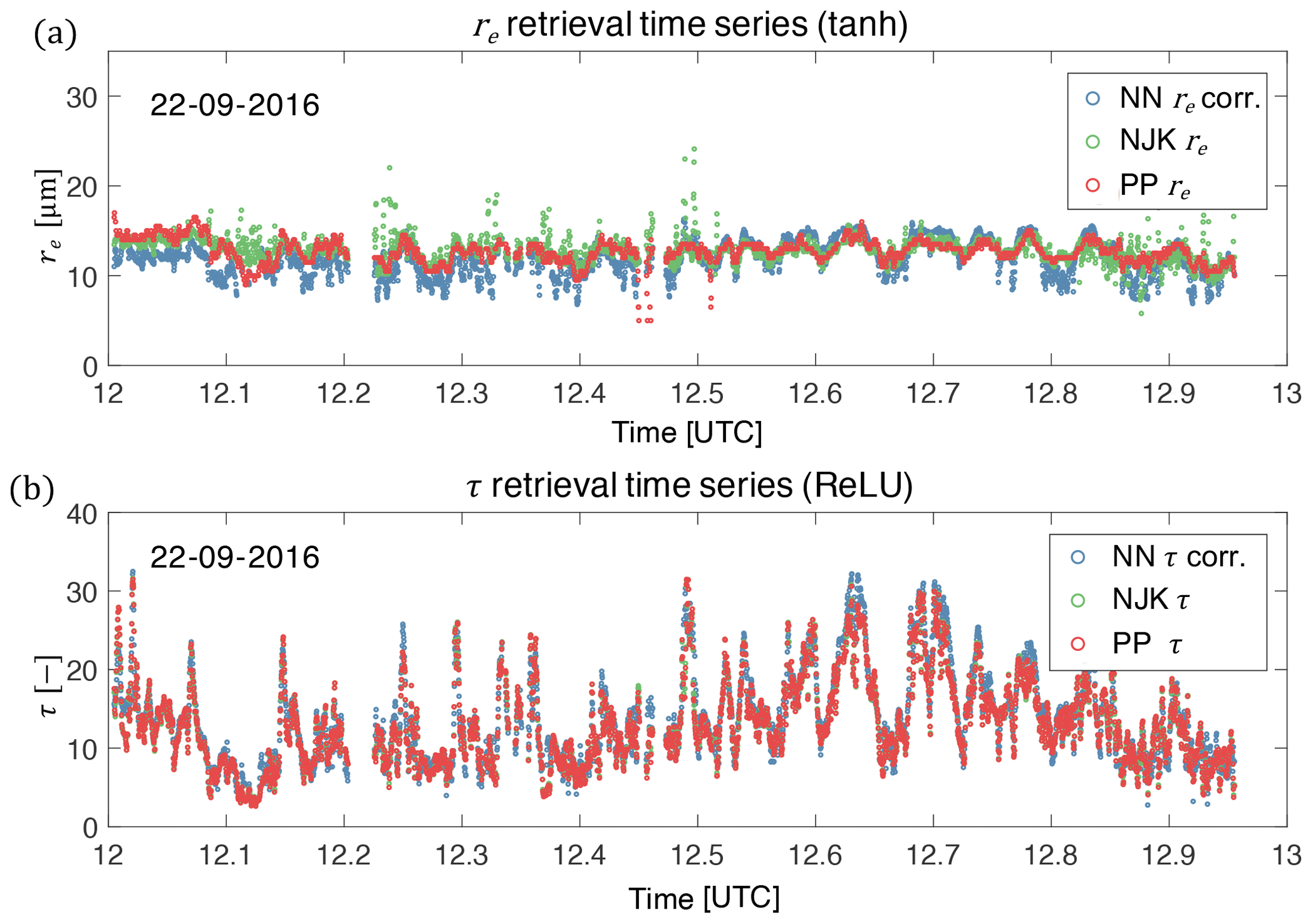
Figure 7A selected time series of re (a) and τ (b) retrievals from NN (blue), NJK (green), and PP (red) methods.
Additionally, we found that the NN retrieval demonstrated some dependence on untrained variables that influence the observational dataset. First, we found a dependence to the fixed cloud-top height assumption (H=1 km) that was made for the ORACLES 2016 training set. This was revealed by comparing our percent retrieval bias (relative to re(PP)) to the HSRL-2 cloud-top height product, as shown in Fig. 8. There is clear covariability between the HSRL-2 cloud-top height and the bias between re(NN) and re(PP). In this example, it appears as though the cloud-top height variation could be associated with a ±20 % variation in the percent retrieval bias depending on the relative error in the cloud-top height assumption. A second sensitivity we observed influenced the τ(NN) retrieval in the presence of above-cloud aerosols. While there was no clear functional dependence, we did observe a handful of cases where the HSRL-2 above-cloud aerosol optical thickness (τACA) was weakly correlated with a reduction in the τ(NN) retrieval.
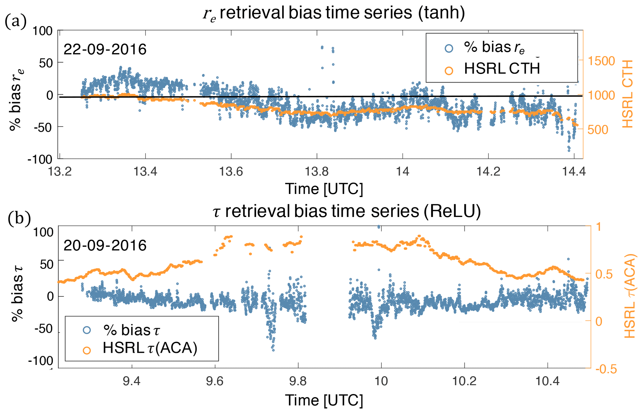
Figure 8Panel (a) is a time series of the percent bias of re(NN) with respect to re(PP) plotted along with the accompanying HSRL-2 CTH time series on top. The solid line going through the center of the panel indicates both zero bias and the CTH assumption of 1 km. Panel (b) shows the time series of the percent bias of τ(NN) with respect to τ(PP) plotted along with the accompanying HSRL-2 τACA. Note that these biases are shown for datasets on different days.
4.3 Results for ORACLES 2017
The ORACLES 2017 campaign data presented a more difficult dataset to work with. Observations that lacked SWIR data and fewer co-located HSRL-2 observations on the days when SWIR data were available reduced the amount of useful intercomparison data. As a consequence, the dataset analyzed here is smaller than 2016 – including 4 d of flights with N=18 159 retrievals that pass all of the analysis criteria discussed in Sect. 2.2. This difficulty also presented an opportunity to test the behavior of a NN retrieval trained without SWIR data at all. To accomplish this, an alternate version of the 2017 ORACLES NN was developed that was trained without SWIR data. Then, the same observational dataset from ORACLES 2017 (namely the data with SWIR observations) was input into both networks either with or without SWIR data accordingly. As shown in Table 4, the NN that excluded SWIR data behaved quite differently than the network trained for SWIR observations.
Table 4Comparison of initial NN output (uncorrected) to PP retrievals during ORACLES 2017. All re retrievals are for a tanh-based network, and all τ retrievals are for a ReLU-based network.
As might be expected, the exclusion of SWIR reflectances has a significant detrimental impact on the NN retrieval of re. Compared to the moderate correlation and RMSE error of NN retrievals with SWIR data (R=0.54 and RMSE=4.77 µm), NN retrievals of re without SWIR data have a very poor correlation and RMSE ( and RMSE=5.86 µm). This behavior is likely attributable to the loss of information content in the SWIR bands, which are strongly absorbed by liquid water droplets and as a consequence are more sensitive to droplet cross section (and therefore re) than the other spectral bands.
Perhaps unexpectedly, the exclusion of SWIR reflectances in the training and observation dataset improves the correlation and RMSE between τ NN retrievals and the other standard RSP retrievals of τ. However, as the comparison of the corrected datasets in Fig. 9 reveals, this story is slightly more complex and nuanced. On the one hand, the histogram regressions clearly show that the τ retrieval with SWIR reflectances (Fig. 9a) is more broadly distributed and exhibits a nonlinear dependency that gets exacerbated for large τ, while the τ retrieval without SWIR reflectances (Fig. 9b) is more tightly distributed and more linearly correlated. This seems to confirm the relationship indicated in the bulk statistics of Table 4. On the other hand, the 1-D histograms reveal that the distribution of the retrieval without SWIR reflectances (Fig. 9d) is mostly densely clustered around bin locations of the training set grid (indicated below as a bar plots). Thus, it appears as though a NN retrieval without SWIR data may be possible if the training set had a higher density of grid points. Another important note is that the slight nonlinear dependence of the τ(NN) retrieval in the SWIR case might be the result of a saturated signal effect. Cloud reflectances are an asymptotic function of τ that saturates at different thicknesses depending on absorption and scattering properties. In particular, the SWIR bands with increased absorption saturate a lower τ than the other bands provided as input to the NN.
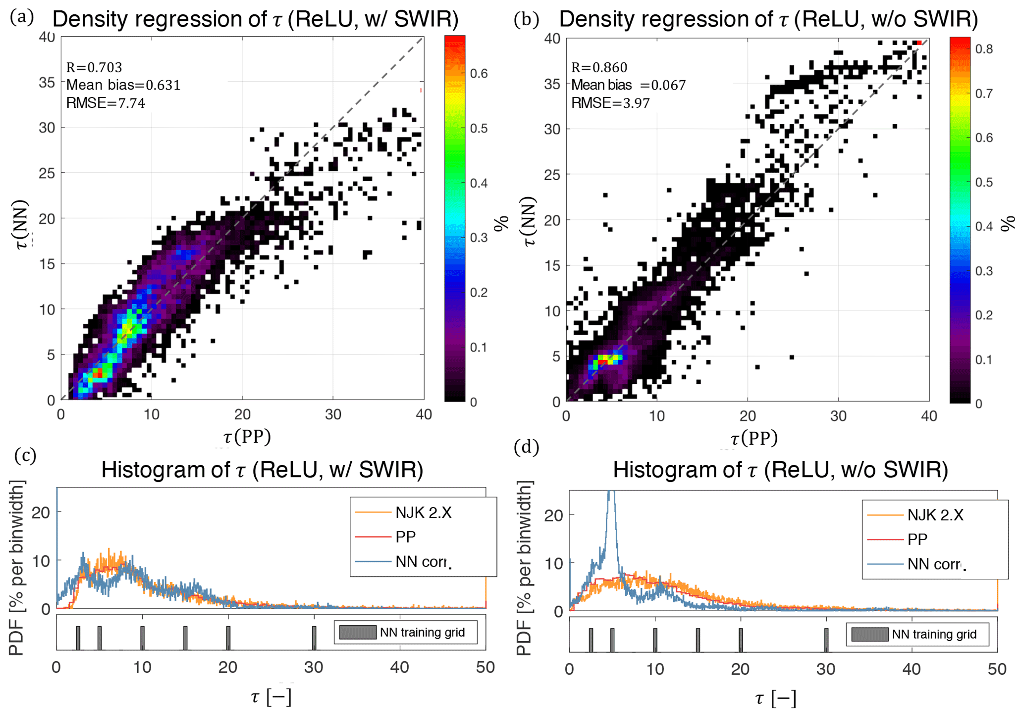
Figure 9Comparisons of corrected NN retrievals against the PP retrievals of τ for the ORACLES 2017 dataset. Panels (a, c) focus on the NN retrieval with SWIR reflectances, while panels (b, d) focus on the NN retrieval without SWIR reflectances. Panels (a, b) are histogram regressions, while panels (c, d) show the corresponding 1-D histogram of the NN retrieval (below which the training grid is shown).
Another interesting finding regarding the NN retrievals in ORACLES 2017 stems from how it compares to the other standard RSP retrievals. In addition to comparison with the PP retrieval as we have highlighted up until now, we have also evaluated comparisons of the NN retrievals against the NJK retrieval. At first glance, the coarse statistical comparison of the initial NN output to the NJK retrieval in Table 5 reveals similar results to those compared to the PP retrieval in Table 4. However, at closer inspection the re retrieval comparison to NJK (with SWIR) has correlations and RMSEs that are moderately better than the results from the PP comparison.
Table 5Comparison of initial NN output to NJK retrievals during ORACLES 2017. All re retrievals are for a tanh-based network, and all τ retrievals are for a ReLU-based network.

Apparently, the ORACLES 2017 NN retrievals of re do not compare as well to the PP retrieval as the results in ORACLES 2016. The histogram regressions in Fig. 10 reveal this clearly, where the comparison to the PP retrieval (panel 10a) shows a clear nonlinearity, whereas the comparison to NJK retrieval (panel 10b) is more linear. Each comparison has similar RMSE but there are also important differences in the distribution of retrievals. In particular, the nonlinear behavior of the comparison to the PP retrieval is reminiscent of the biases shown previously during the comparison of NJK and PP to one another directly in Fig. 2, where there were also large, high biases in the NJK retrieval for small and large droplet size regimes. Previously, we concluded that this difference was associated with thin (τ<3) or broken clouds. The increased relative occurrence of thin and broken clouds that characterized the observations made during ORACLES 2017 appears to be the primary source of this behavior. This population of clouds is most susceptible to biases that are coupled to spatial resolution – specifically unresolved cloud inhomogeneity and resolved 3-D radiative effects. These effects are known to have a more severe influence on the NJK re retrieval than on the PP retrieval of re (Miller et al., 2016, 2018). Interestingly, because the NN retrieval is ingesting reflectances that may be biased by these effects, the NN retrieval more closely resembles the results of the NJK retrieval rather than the PP retrieval. This appears to indicate, at least for the ORACLES 2017 dataset, that the NN places are influenced strongly by biased total reflectances, particularly for the optically thin clouds that were often observed.
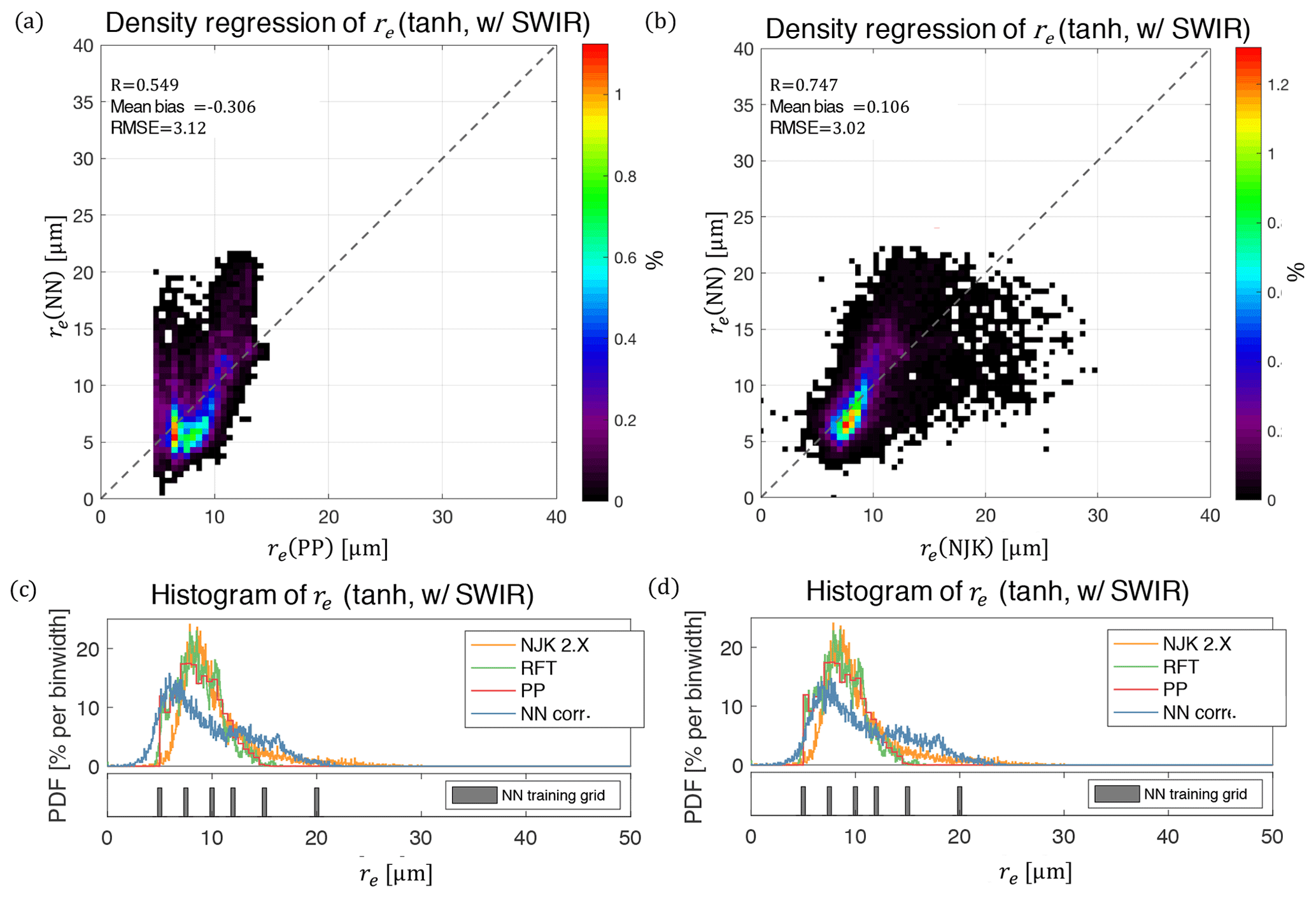
Figure 10Histogram regressions of re retrievals that compare NN to PP retrievals (a) and NN to NJK retrievals (b). Below are the 1-D histograms of the different NN-corrected retrievals using different reference retrievals (PP, c; NJK d) for the linear correction of the initial NN output.
Looking at the flight track time series the observed spatial variability of the ORACLES 2017 NN retrieval in Fig. 11 reveals some similarities to the ORACLES 2016 cases examined previously. In particular, the spatial variability of the ORACLES 2017 NN retrievals of τ appears similar to the results shown previously in Fig. 7. However, looking more closely at the re time series reveals that there is a clear deviation of both the NN and NJK retrievals around a gap in the cloud at approximately 10.5 UTC – a behavior not observed in the PP retrieval. This is evidence that cloud inhomogeneity and thin clouds (τ<3) are indeed the source of the biases observed in both the NN and NJK retrievals in this dataset. Additionally, there are notable deviations of the NN retrieval of re away from other RSP retrievals in the proximity of steep increases or decreases in τ (e.g., around 10.7 or 10.85 UTC). This behavior could be a consequence of stronger 3-D radiative effects in the shorter-wavelength spectral bands that are not used by the NJK retrieval but are a part of this NN framework (e.g., λ=0.410 µm).
While the ORACLES 2016 NN retrievals exhibited correlation to some untrained variables like cloud-top height and above-cloud aerosol optical thickness, the results from ORACLES 2017 did not reveal any meaningful correlations with ACA optical thickness. Additionally, there was no clear sensitivity of the new network to cloud-top height. Indicating that training with the flight altitude as a variable during training had a positive impact on the retrieval outcomes for this dataset.
Overall, the results of this study demonstrate that a multiangular polarimetric neural network cloud property retrieval can produce results that are statistically similar to other existing RSP cloud retrievals. Defining the input layer of the NN required careful consideration of the particularities of multiangular polarimetric data. For example, we found that appropriately weighting of observations that have vastly different uncertainties was quite important because total (I) and polarized (DoLP) observations differ from one another by an order of magnitude in both value and uncertainty. Additionally, we constructed a deeper network architecture and created a more efficient network that could operate on the entire observation vector itself, rather than on a reduced input vector. After making these input vector decisions, each retrieval was performed using a separate network architecture, each giving the best results for the given variable (re or τ). Specifically, we found that networks using different activation functions performed better for retrievals of τ and re – namely, the network using tanh for re retrievals and the network using ReLU for τ retrievals. In addition to using different networks for re and τ retrievals, the inherent differences between the ORACLES 2016 and 2017 datasets required us to develop different networks for each year that were built using training data tailored for the observation conditions. This effort was complicated by the fact that the two datasets differed significantly, with many more broken and inhomogeneous clouds present in the ORACLES 2017 dataset. This presented a challenge for the NN and other RSP retrievals but also an opportunity for us to learn how the NN behaved in a larger variety of conditions.
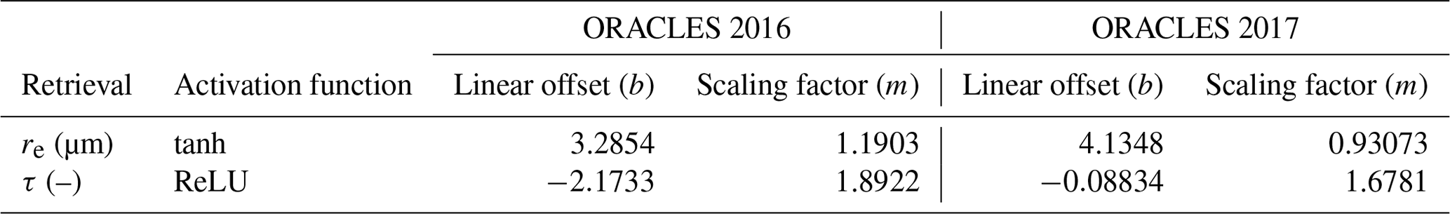
As discussed in Sect. 4.1, the initial output of the NN exhibited a clear systematic linear offset relative to the other RSP standard retrievals. This was especially true for the re retrieval, which had an offset bias of about 3 µm. To create a dataset that was more consistent with the other RSP retrievals, we arbitrarily linearly corrected the NN retrieval datasets by linear regression to the RSP PP retrieval for a limited sampling of retrievals. Afterwards, the linear correction was applied to the full dataset and the results were again compared to other RSP cloud retrievals using the correlations and RMSE statistics as a meaningful evaluation of the retrievals quality. However, the source of the linear offset bias likely stems from a difference in the data used in the training set and the observations made by the instrument. The simplest explanation for this difference is associated with above-cloud gaseous absorption that was not modeled in the NN training sets. The absorption of well-mixed gases (e.g., CO2 and CH4) and trace gases (e.g., water vapor (WV), NO2, and O3) can vary significantly within some of the spectral bands of RSP – of particular note is strong absorption by CO2 and CH4 in two SWIR bands where much of the sensitivity to cloud droplet size information is contained. Additionally, the absorption of these gases also increases with increasing view angle as the light scattered to the detector passes through a longer atmospheric path at oblique viewing angles. To test the impact of atmospheric absorption we re-examined a pair of cases of atmospherically corrected RSP data and compared them to our original NN retrievals time series data from 2016 and 2017 shown in Figs. 7 and 11. The modeled atmosphere was built using RSP retrievals of above-cloud WV, in addition to MERRA-2 reanalysis column NO2, O3, and subsequent assumptions regarding well-mixed gases and vertical profiles based on the U.S. Standard Atmosphere (National Aeronautics and Space Administration et al., 1976). Cloud-top height measurements from HSRL2 were used to define cloud top and subsequently calculate the above-cloud impact on the absorption of the two-way transmitted reflectance. The re retrievals from the initial NN output (not linearly adjusted) that is obtained using the atmospherically corrected reflectances for ORACLES 2016 and ORACLES 2017 networks are compared to the original scaled NN retrievals and the polarimetric RSP retrieval in Fig. 12. It is evident that the atmospheric correction largely serves to reduce the re retrieval globally to a value that is more in line with the polarimetric retrieval – cutting the offset bias nearly in half. This is likely due to the correction for absorption in the SWIR bands as well as the correction to the angular distribution of reflectance due to large view angles having significantly more absorption. It is also good to note the atmospheric correction has very little impact on the NN retrieval of τ, which did not have a significant offset bias. It should also be noted that after correcting the observational input, the tanh-based network retrieval of τ improved markedly – indicating that this activation function may be more useful than we found previously. These initial results are promising, because they largely do not change the variability in the time series and as a consequence validate our original linear correction approach. The atmospherically corrected reflectance observations were used to produce the publicly available NN retrieval stored in our archive (refer to the Data availability section).

Figure 11A selected time series of re (a) and τ (b) retrievals from NN (blue), NJK (green), and PP (red) methods.
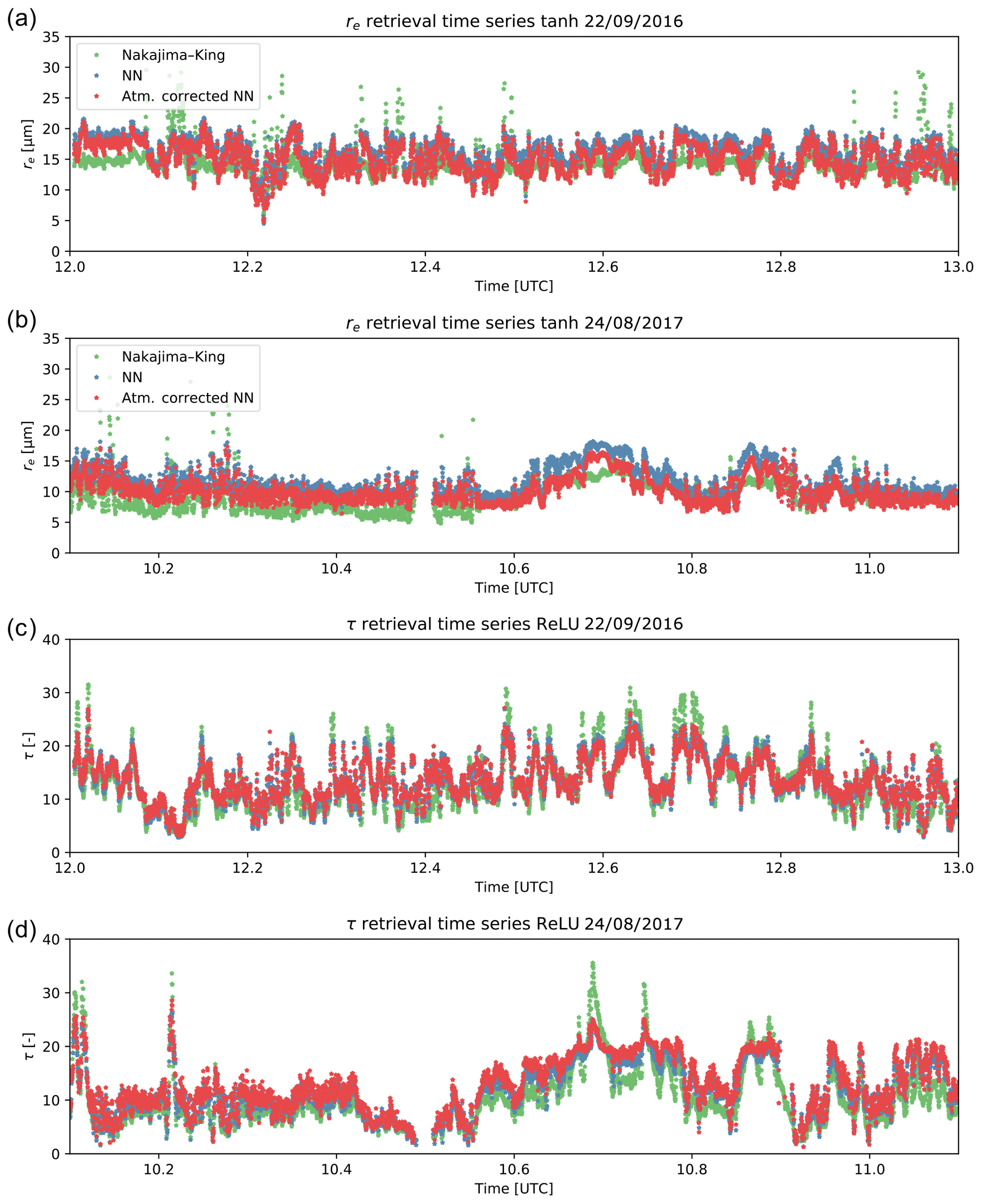
Figure 12Time series comparisons of NJK retrievals (green), uncorrected NN retrievals (blue), and NN retrievals using atmospherically corrected reflectances. Panels (a, b) focus on re retrievals from ORACLES 2016 (a) and 2017 (b), while panels (c, d) present the τ time series from ORACLES 2016 (c) and 2017 (d).
Table 6A summary of the properties of the archived RSP NN retrieval. All re retrievals are for a tanh-based network, and all τ retrievals are for a ReLU-based network. The linear corrections applied to the initial NN output are recorded here so that one could replicate results presented in this paper.
Comparisons of the NN retrieval to the existing RSP cloud retrievals during ORACLES revealed reasonable results. In particular, the ORACLES 2016 dataset showed comparisons of neural network retrievals (NN) to the RSP polarimetric retrievals (PP) that had correlations for re and τ of R=0.756 and R=0.950, respectively, while the RMSEs for re and τ were 1.74 µm and 1.82, respectively. The results of this comparison are of similar quality to the comparison of the standard RSP PP and NJK retrievals to one another in Fig. 2. In contrast to these results, the ORACLES 2017 dataset fared poorly, with correlations and RMSEs of NN retrievals of re (R=0.54 and RMSE=4.77 µm) and τ (R=0.785 and RMSE=5.61) that were much worse. Though, based on the comparisons of the standard RSP PP and NJK retrievals of re, this was to be expected due to the increased prevalence of optically thin (τ<3) clouds observed in the ORACLES 2017 data. As a consequence, the NN retrievals of re during this year more closely resemble the systematically high-biased NJK retrievals. It is, however, surprising that the τ retrieval performed so poorly for this dataset. It appears to be the result of a strong nonlinear behavior with increasing τ. We found that if we attempted to retrieve τ using an input vector that excluded the SWIR data, then the τ retrieval statistics improved significantly (R=0.908 and RMSE=3.08). However, this SWIR-free NN retrieval exhibited an undesirable training set bin-seeking behavior that may possibly be avoided if we trained with a denser grid of training set variables. In a general sense, our training sets in this study are relatively small (≈250 000 grid points) compared to other neural network remote sensing studies which were trained on millions to even tens of millions of datapoints (Di Noia et al., 2019; Strandgren et al., 2017; Kox et al., 2014).
The NN was trained using a synthetic dataset that made some significant assumptions about the types of scenes that would be observed. The first type of assumption relates to the structure of the forward model itself (i.e., assuming that clouds are plane-parallel and internally homogeneous to simplify to a 1-D radiative transfer problem). As a consequence, the cloud is assumed to be vertically homogeneous, which could cause issues due to the different vertical information contained in polarized reflectances which scatter from a shallow layer at the cloud top, while the total radiances contain information from deeper within the cloud. The second type of assumption is about the state of the atmosphere itself (i.e., using a fixed cloud-top height). Another example of this type of assumption is that the observations in the training set exclusively consider the presence of clear cloudy scenes, with no aerosols above the cloud. We cannot do much about the first type of assumption, as cloud retrievals are subject to the possible influence of inhomogeneity and 3-D radiative effects – which usually have a greater impact on total reflectance-based retrievals than on polarimetric retrievals (Miller, 2017). On the other hand, the second type of assumption is something that can be further explored in future studies by incorporating a more complete description of the atmospheric state in the training dataset. We experimented with one such assumption of this type by training the network for ORACLES 2017 to account for variability in the separation between the Aircraft altitude and the cloud-top height. As a consequence the retrievals for the ORACLES 2017 dataset did not demonstrate the same systematic bias in re as a function of cloud-top height that we observed in the ORACLES 2016 dataset. We have not yet extensively tested how above-cloud aerosols influence the results of the NN retrievals shown here. There was some indication in Fig. 8 that ACA could lead to slight low biases in τ retrievals compared to the RSP PP retrieval, though in that instance both retrievals of τ should be impacted by the ACA layer. From previous studies based on the bispectral (NJK) retrieval, this behavior is expected in the presence of an absorbing ACA layer (Meyer et al., 2013). In order to account for this effect, however, a simultaneous retrieval of aerosol and cloud optical thickness would be required, which would be a topic for a future study.
The NN approach outlined here does come with some particular challenges that are unique relative to other approaches (e.g., LUT-based search, curve fitting, iterative least squares, etc.): it is not designed to obtain a “best fit” between simulations and observations for each observation. Rather, it is designed to obtain a best fit for a population of training data and later generalize that behavior to different observational input data. As a consequence, analyzing the behavior of NN retrievals requires carefully developing an understanding of the training and input datasets and their potential differences. However, despite this potential difficulty, the NN retrieval was shown here to provide reasonable results, lending support to the idea that a NN retrieval could provide a quick first guess to other numerically rigorous retrievals (Di Noia et al., 2015). Another interesting feature of the approach we have taken for the NN retrieval is that it makes full use of the large information content of multiangular polarimetry, using all the total and polarized reflectances, numerous wavelengths, and viewing geometries in the same retrieval. This is unlike the other RSP retrievals, which typically make use of a limited wavelengths and either polarized or total reflectance observations. As a consequence of using both total and polarized reflectances, we found that the NN retrieval was sometimes behaving more like the PP retrieval (when the clouds were optically thick and more homogeneous) and sometimes behaving more like the NJK retrieval (when clouds were thinner and less homogeneous). It is possible that this is an indication that the NN is detrimentally influenced by biases in total reflectances associated to 3-D radiative effects and unresolved cloud inhomogeneity that also impacts the NJK retrieval. These biases in total reflectance can be most severe for thin and broken clouds. This brings us to another weakness: the analysis of this study hinges on the comparison of retrievals to other retrievals. Without a true baseline reference, we only have comparisons between different approaches, which comes with its own caveats and sources of bias. This is specifically important in the case when both retrievals are not considering a large component of the observed system (e.g., the presence of an above-cloud aerosol layer).
In the future we intend to extend this NN retrieval study in a few aspects. First, we endeavor to redefine our approach to developing the training set. Rather than use a fixed grid training set as we did in this study, we would like to use an approach that is more flexible and allows us to train more in the regions of state space that occur most often. One of the ways to do this is to implement importance or occurrence sampling in the training set. Importance sampling requires the user to define the full distribution of a priori cloud and aerosol parameters in the state space. Then the user specifies a number of training samples desired and then a value is randomly sampled from the distributions of each of the atmospheric state variables, leading to numerous unique combinations of atmospheric simulations. This results in a training set that more accurately represents the underlying state space of the observational dataset and avoids the binned retrieval issues we saw in some of the NN retrievals in this study. Second, because we saw improvement in the NN results when we corrected for atmospheric absorption, we intend to improve our approach to atmospheric correction – making the input observations more closely resemble the synthetic training dataset. Third, with our understanding of the cloud retrieval problem on firmer ground, we hope to extend the NN retrieval approaches discussed here to the retrieval of above-cloud aerosol properties. Finally, we would also like to demonstrate that this NN first guess can indeed accelerate a rigorous optimal estimation retrieval of above-cloud aerosol properties by providing an accurate a priori estimate of the retrieval space that should be explored. The lessons learned from this study can hopefully help in other applications of machine learning to remote sensing data. The full RSP NN retrieval product can be accessed from the DOI in the data availability statement below.
The RSP NN cloud retrievals from all ORACLES field campaigns can be found at the
following locations –
https://doi.org/10.5067/Suborbital/ORACLES/ER2/2016_V2 (ORACLES Science Team, 2017);
https://doi.org/10.5067/Suborbital/ORACLES/P3/2017_V2 (ORACLES Science Team, 2019a);
https://doi.org/10.5067/Suborbital/ORACLES/P3/2018_V2 (ORACLES Science Team, 2019b). All other RSP
retrieval products can also be accessed at: https://data.giss.nasa.gov/pub/rsp/ (last access: June 2020) (RSP Science Team, 2020). Finally,
all ORACLES data will also be permanently archived in the NASA Langley ASDC DAAC, which can be
accessed at: 10.5067/ASDC_DAAC/ORACLES_AerosolCloud (ORACLES Science Team, 2020). Interested
users are encouraged to contact the authors with questions and advice on accessing these different
datasets.
DM, KK, and MS-R drafted the manuscript together. The network architecture was defined and developed by MS-R, while the simulated RSP training dataset was generated by KK, and the input standardization and uncertainty scheme was created by DM. Primary analysis and data processing were handled by DM. Integration of RSP measurements, retrievals, and atmospheric correction in this study was supported by BC, MA, BvD, and AW. All authors contributed to the editing of the article.
The authors declare that they have no conflict of interest.
This article is part of the special issue “New observations and related modelling studies of the aerosol–cloud–climate system in the Southeast Atlantic and southern Africa regions (ACP/AMT inter-journal SI)”. It is not associated with a conference.
The authors would like to acknowledge NASA funding and support for the ORACLES project. We would like the thank the ORACLES ER-2 and P-3 aircrew for its support in the field. Additionally, The authors are grateful to Sharon Burton, Johnathan Hair, and Richard Ferrare of the NASA Langley HSRL-2 team for making their data available and providing feedback on our data.
This research has been supported by NASA (grant no. NNH13ZDA001N-EVS2). Daniel J. Miller's research was supported by an appointment to the NASA Postdoctoral Program at the NASA Goddard Space Flight Center, administered by Universities Space Research Association (USRA) under contract with NASA.
This paper was edited by Paquita Zuidema and reviewed by three anonymous referees.
Abadi, M., Agarwal, A., Barham, P., Brevdo, E., Chen, Z., Citro, C., Corrado, G. S., Davis, A., Dean, J., Devin, M., Ghemawat, S., Goodfellow, I., Harp, A., Irving, G., Isard, M., Jia, Y., Jozefowicz, R., Kaiser, L., Kudlur, M., Levenberg, J., Mane, D., Monga, R., Moore, S., Murray, D., Olah, C., Schuster, M., Shlens, J., Steiner, B., Sutskever, I., Talwar, K., Tucker, P., Vanhoucke, V., Vasudevan, V., Viegas, F., Vinyals, O., Warden, P., Wattenberg, M., Wicke, M., Yu, Y., and Zheng, X.: TensorFlow: Large-Scale Machine Learning on Heterogeneous Distributed Systems, arXiv [preprint], arxiv:1603.04467v2, 2016. a
Adebiyi, A. A. and Zuidema, P.: The role of the southern African easterly jet in modifying the southeast Atlantic aerosol and cloud environments, Q. J. Roy. Meteorol. Soc., 142, 1574–1589, 2016. a
Alexandrov, M. D., Cairns, B., Emde, C., Ackerman, A. S., and van Diedenhoven, B.: Accuracy assessments of cloud droplet size retrievals from polarized reflectance measurements by the research scanning polarimeter, Remote Sens. Environ., 125, 92–111, 2012a. a, b, c, d, e
Alexandrov, M. D., Cairns, B., and Mishchenko, M. I.: Rainbow Fourier transform, J. Quant. Spectrosc. Ra., 113, 2521–2535, 2012b. a, b
Alexandrov, M. D., Cairns, B., Wasilewski, A. P., Ackerman, A. S., McGill, M. J., Yorks, J. E., Hlavka, D. L., Platnick, S., Thomas Arnold, G., van Diedenhoven, B., Chowdhary, J., Ottaviani, M., and Knobelspiesse, K. D.: Liquid water cloud properties during the Polarimeter Definition Experiment (PODEX), Remote Sens. Environ., 169, 20–36, 2015. a
Alexandrov, M. D., Cairns, B., van Diedenhoven, B., Ackerman, A. S., Wasilewski, A. P., McGill, M. J., Yorks, J. E., Hlavka, D. L., Platnick, S., and Arnold, G. T.: Polarized view of supercooled liquid water clouds, Remote Sens. Environ., 181, 96–110, 2016. a, b
Bréon, F. M. and Goloub, P.: Cloud droplet effective radius from spaceborne polarization measurements, Geophys. Res. Lett., 25, 1879–1882, 1998. a
Burton, S. P., Cook, A. L., Hostetler, C. A., Müller, D., Harper, D. B., Chemyakin, E. V., Smith, J. A., Hair, J. W., Fenn, M. A., Saide, P. E., Ferrare, R. A., Scola, S., and Seaman, S. T.: Calibration of a high spectral resolution lidar using a Michelson interferometer, with data examples from ORACLES, Appl. Opt., 57, 6061–6075, 2018. a
Cairns, B. and Chowdhary, J.: Aerosol and Cloud Environmental Data Records: Aerosol Polarimetry Sensor Algorithm Theoretic Basis Document, technical report, NASA Headquarters, Washington, D.C., 2003. a
Chollet, F.: Deep Learning with Python, 1st edn., Manning Publications Co., Greenwich, CT, USA, 2017. a
Chowdhary, J. and Cairns, B.: Case studies of aerosol retrievals over the ocean from multiangle, multispectral photopolarimetric remote sensing data, J. Atmos. Sci., 59, 383–397, 2002. a
Chowdhary, J., Cairns, B., Mishchenko, M., and Travis, L.: Retrieval of aerosol properties over the ocean using multispectral and multiangle Photopolarimetric measurements from the Research Scanning Polarimeter, Geophys. Res. Lett., 28, 243–246, 2001. a
Chowdhary, J., Cairns, B., Mishchenko, M. I., Cota, G. F., Rutledge, K., Holben, B. N., Russell, E., Hobbs, P. V., Cota, G. F., Redemann, J., Rutledge, K., Holben, B. N., and Russell, E.: Retrieval of Aerosol Scattering and Absorption Properties from Photopolarimetric Observations over the Ocean during the CLAMS Experiment, J. Atmos. Sci., 62, 1093–1117, 2005a. a
Chowdhary, J., Cairns, B., Mishchenko, M. I., and Travis, L. D.: Using multi-angle multispectral photo-polarimetry of the NASA Glory mission to constrain optical properties of aerosols and clouds: results from four field experiments, in: Sensors, Systems, and Next-Generation Satellites IX, p. 59780G, International Society for Optics and Photonics, 2005b. a
Chowdhary, J., Cairns, B., and Travis, L. D.: Contribution of water-leaving radiances to multiangle, multispectral polarimetric observations over the open ocean: bio-optical model results for case 1 waters, Appl. Opt., 45, 5542–5567, 2006. a
Chowdhary, J., Cairns, B., Waquet, F., Knobelspiesse, K., Ottaviani, M., Redemann, J., Travis, L., and Mishchenko, M.: Sensitivity of multiangle, multispectral polarimetric remote sensing over open oceans to water-leaving radiance: Analyses of RSP data acquired during the MILAGRO campaign, Remote Sens. Environ., 118, 284–308, 2012. a
Costantino, L. and Bréon, F.-M.: Aerosol indirect effect on warm clouds over South-East Atlantic, from co-located MODIS and CALIPSO observations, Atmos. Chem. Phys., 13, 69–88, https://doi.org/10.5194/acp-13-69-2013, 2013. a
De Haan, J. F., Bosma, P. B., and Hovenier, J. W.: The adding method for multiple scattering calculations of polarized light, Astron. Astrophys., 183, 371–391, 1987. a
Deirmendjian, D.: Scattering and polarization properties of water clouds and hazes in the visible and infrared, Appl. Opt., 3, 187–196, 1964. a
Del Frate, F. and Schiavon, G.: Nonlinear principal component analysis for the radiometric inversion of atmospheric profiles by using neural networks, IEEE T. Geosci. Remote Sens., 37, 2335–2342, 1999. a
Del Frate, F., Iapaolo, M., Casadio, S., Godin-Beekmann, S., and Petitdidier, M.: Neural networks for the dimensionality reduction of GOME measurement vector in the estimation of ozone profiles, J. Quant. Spectrosc. Ra., 92, 275–291, 2005. a
Di Noia, A., Hasekamp, O. P., van Harten, G., Rietjens, J. H. H., Smit, J. M., Snik, F., Henzing, J. S., de Boer, J., Keller, C. U., and Volten, H.: Use of neural networks in ground-based aerosol retrievals from multi-angle spectropolarimetric observations, Atmos. Meas. Tech., 8, 281–299, https://doi.org/10.5194/amt-8-281-2015, 2015. a, b, c
Di Noia, A., Hasekamp, O. P., van Diedenhoven, B., and Zhang, Z.: Retrieval of liquid water cloud properties from POLDER-3 measurements using a neural network ensemble approach, Atmos. Meas. Tech., 12, 1697–1716, https://doi.org/10.5194/amt-12-1697-2019, 2019. a, b
Formenti, P., D'Anna, B., Flamant, C., Mallet, M., Piketh, S. J., Schepanski, K., Auriol, F., Brogniez, G., Burnet, F., Chaboureau, J.-P., Chauvigné, A., Chazette, P., Denjean, C., Desboeufs, K., Doussin, J.-F., Elguindi, N., Feuerstein, S., Gaetani, M., Giorio, C., Klopper, D., Mallet, M. D., Nabat, P., Monod, A., Solmon, F., Namwoonde, A., Chikwililwa, C., Mushi, R., Welton, E. J., Holben, B., D'Anna, B., Flamant, C., Mallet, M., Piketh, S. J., Schepanski, K., Waquet, F., Auriol, F., Brogniez, G., Burnet, F., Chaboureau, J.-P., Chauvigné, A., Chazette, P., Denjean, C., Desboeufs, K., Doussin, J.-F., Elguindi, N., Feuerstein, S., Gaetani, M., Giorio, C., Klopper, D., Mallet, M. D., Nabat, P., Monod, A., Solmon, F., Namwoonde, A., Chikwililwa, C., Mushi, R., and Welton, E. J.: The Aerosols, Radiation and Clouds in Southern Africa Field Campaign in Namibia: Overview, Illustrative Observations, and Way Forward, B. Am. Meteorol. Soc., 100, 1277–1298, 2019. a
Hair, J. W., Hostetler, C. A., Harper, D. B., Cook, A. L., Hovis, F. E., Izquierdo, L. R., Ferrare, R. A., Mack, T. L., and Welch, W.: Airborne High Spectral Resolution Lidar for profiling aerosol optical properties, Appl. Opt., 47, 6734–6752, 2008. a
Hansen, J. E.: Multiple scattering of polarized light in planetary atmospheres part II. Sunlight reflected by terrestrial water clouds, J. Atmos. Sci., 28, 1400–1426, 1971. a
Hansen, J. E. and Travis, L. D.: Light scattering in planetary atmospheres, Space Sci. Rev., 16, 527–610, 1974. a, b, c
Hovenier, J. W.: Multiple scattering of polarized light in planetary atmospheres, Astron. Astrophys., 13, 7–29, 1971. a
IPCC: Climate Change: The Assessment Reports of the Intergovernmental Pane on Climate Change, 2013. a
Kingma, D. P. and Ba, J.: Adam: A Method for Stochastic Optimization, arXiv [preprint], arXiv:1412.6980, 2014. a
Knobelspiesse, K., Cairns, B., Ottaviani, M., Ferrare, R., Hair, J., Hostetler, C., Obland, M., Rogers, R., Redemann, J., Shinozuka, Y., Clarke, A., Freitag, S., Howell, S., Kapustin, V., and McNaughton, C.: Combined retrievals of boreal forest fire aerosol properties with a polarimeter and lidar, Atmos. Chem. Phys., 11, 7045–7067, https://doi.org/10.5194/acp-11-7045-2011, 2011a. a
Knobelspiesse, K., Cairns, B., Redemann, J., Bergstrom, R. W., and Stohl, A.: Simultaneous retrieval of aerosol and cloud properties during the MILAGRO field campaign, Atmos. Chem. Phys., 11, 6245–6263, https://doi.org/10.5194/acp-11-6245-2011, 2011b. a, b, c
Knobelspiesse, K., Cairns, B., Jethva, H., Kacenelenbogen, M., Segal-Rosenheimer, M., and Torres, O.: Remote sensing of above cloud aerosols, in: Light Scattering Reviews, Vol. 9, Springer Berlin Heidelberg, Berlin, Heidelberg, pp. 167–210, 2015. a
Knobelspiesse, K., Tan, Q., Bruegge, C., Cairns, B., Chowdhary, J., van Diedenhoven, B., Diner, D., Ferrare, R., van Harten, G., Jovanovic, V., Ottaviani, M., Redemann, J., Seidel, F., and Sinclair, K.: Intercomparison of airborne multi-angle polarimeter observations from the Polarimeter Definition Experiment, Appl. Opt., 58, 650–669, 2019. a, b
Koch, D. and Del Genio, A. D.: Black carbon semi-direct effects on cloud cover: review and synthesis, Atmos. Chem. Phys., 10, 7685–7696, https://doi.org/10.5194/acp-10-7685-2010, 2010. a
Kox, S., Bugliaro, L., and Ostler, A.: Retrieval of cirrus cloud optical thickness and top altitude from geostationary remote sensing, Atmos. Meas. Tech., 7, 3233–3246, https://doi.org/10.5194/amt-7-3233-2014, 2014. a
Krizhevsky, A., Sutskever, I., and Hinton, G. E.: ImageNet Classification with Deep Convolutional Neural Networks, papers.nips.cc, pp. 1097–1105, 2012. a
LeCun, Y., Boser, B., Denker, J. S., Henderson, D., Howard, R. E., Hubbard, W., and Jackel, L. D.: Backpropagation Applied to Handwritten Zip Code Recognition, Neural Computation, 1, 541–551, 1989. a, b
LeCun, Y., Bottou, L., Orr, G., and Müller, K. R.: Neural Networks: Tricks of the trade, Efficient BackProp, Springer, 1998. a
Lu, Z., Liu, X., Zhang, Z., Zhao, C., Meyer, K., Rajapakshe, C., Wu, C., Yang, Z., and Penner, J. E.: Biomass smoke from southern Africa can significantly enhance the brightness of stratocumulus over the southeastern Atlantic Ocean, Proc. Natl. Acad. Sci. USA, 115, 2924–2929, 2018. a
Meyer, K., Platnick, S., Oreopoulos, L., and Lee, D.: Estimating the direct radiative effect of absorbing aerosols overlying marine boundary layer clouds in the southeast Atlantic using MODIS and CALIOP, J. Geophys. Res.-Atmos., 118, 4801–4815, 2013. a, b, c, d
Miller, D. J.: Satellite Simulator Studies of the Impact of Cloud Inhomogeneity on Passive Cloud Remote Sensing Retrievals, Ph.D. thesis, ProQuest Dissertations Publishing, University of Maryland, Baltimore County, 2017. a
Miller, D. J., Zhang, Z., Ackerman, A. S., Platnick, S., and Baum, B. A.: The impact of cloud vertical profile on liquid water path retrieval based on the bispectral method: A theoretical study based on large-eddy simulations of shallow marine boundary layer clouds, J. Geophys. Res.-Atmos., 121, 4122–4141, 2016. a
Miller, D. J., Zhang, Z., Platnick, S., Ackerman, A. S., Werner, F., Cornet, C., and Knobelspiesse, K.: Comparisons of bispectral and polarimetric retrievals of marine boundary layer cloud microphysics: case studies using a LES–satellite retrieval simulator, Atmos. Meas. Tech., 11, 3689–3715, https://doi.org/10.5194/amt-11-3689-2018, 2018. a, b, c, d, e
Mishchenko, M. I., Cairns, B., Travis, L. D., Kopp, G., Schueler, C. F., Fafaul, B. A., Hooker, R. J., Maring, H. B., Itchkawich, T., Hansen, J. E., Kopp, G., Schueler, C. F., Fafaul, B. A., Hooker, R. J., Maring, H. B., and Itchkawich, T.: Accurate Monitoring of Terrestrial Aerosols and Total Solar Irradiance: Introducing the Glory Mission, B. Am. Meteorol. Soc., 88, 677–691, 2007. a, b
Nakajima, T. and King, M. D.: Determination of the optical thickness and effective particle radius of clouds from reflected solar radiation measurements. Part I: Theory, J. Atmos. Sci., 47, 1878–1893, 1990. a, b
National Aeronautics and Space Administration, National oceanic and atmospheric administration (US), and United States Air Force: U.S. standard atmosphere, 1976, U.S. Government Printing Office, 1976. a
ORACLES Science Team: Suite of Aerosol, Cloud, and Related Data Acquired Aboard ER2 During ORACLES 2016, Version 2, NASA Ames Earth Science Project Office, https://doi.org/10.5067/Suborbital/ORACLES/ER2/2016_V2, 2017. a
ORACLES Science Team: Suite of Aerosol, Cloud, and Related Data Acquired Aboard P3 During ORACLES 2017, Version 2, NASA Ames Earth Science Project Office, https://doi.org/10.5067/Suborbital/ORACLES/P3/2017_V2, 2019a. a
ORACLES Science Team: Suite of Aerosol, Cloud, and Related Data Acquired Aboard P3 During ORACLES 2018, Version 2, NASA Ames Earth Science Project Office, https://doi.org/10.5067/Suborbital/ORACLES/P3/2018_V2, 2019b. a
ORACLES Science Team: Suite of Aerosol, Cloud, and Related Data Acquired During ORACLES Campaign, Version 1, NASA Langley ASDC DAAC, 10.5067/ASDC_DAAC/ORACLES_AerosolCloud, 2020. a
Ottaviani, M., Cairns, B., Chowdhary, J., van Diedenhoven, B., Knobelspiesse, K., Hostetler, C., Ferrare, R., Burton, S., Hair, J., Obland, M. D., and Rogers, R.: Polarimetric retrievals of surface and cirrus clouds properties in the region affected by the Deepwater Horizon oil spill, Remote Sens. Environ., 121, 389–403, 2012. a
Ottaviani, M., van Diedenhoven, B., and Cairns, B.: Photopolarimetric retrievals of snow properties, The Cryosphere, 9, 1933–1942, https://doi.org/10.5194/tc-9-1933-2015, 2015. a
Painemal, D., Kato, S., and Minnis, P.: Boundary layer regulation in the southeast Atlantic cloud microphysics during the biomass burning season as seen by the A-train satellite constellation, J. Geophys. Res.-Atmos., 119, 11288–11302, 2014. a
Peralta, R. J., Nardell, C., Cairns, B., Russell, E. E., Travis, L. D., Mishchenko, M. I., Fafaul, B. A., and Hooker, R. J.: Aerosol polarimetry sensor for the Glory Mission, in: MIPPR 2007: Automatic Target Recognition and Image Analysis; and Multispectral Image Acquisition, p. 67865L, International Society for Optics and Photonics, 2007. a
Persh, S., Shaham, Y. J., Benami, O., Cairns, B., Mishchenko, M. I., Hein, J. D., and Fafaul, B. A.: Ground performance measurements of the Glory Aerosol Polarimetry Sensor, in: Earth Observing Systems XV, p. 780703, International Society for Optics and Photonics, 2010. a
Pistone, K., Redemann, J., Doherty, S., Zuidema, P., Burton, S., Cairns, B., Cochrane, S., Ferrare, R., Flynn, C., Freitag, S., Howell, S. G., Kacenelenbogen, M., LeBlanc, S., Liu, X., Schmidt, K. S., Sedlacek III, A. J., Segal-Rozenhaimer, M., Shinozuka, Y., Stamnes, S., van Diedenhoven, B., Van Harten, G., and Xu, F.: Intercomparison of biomass burning aerosol optical properties from in situ and remote-sensing instruments in ORACLES-2016, Atmos. Chem. Phys., 19, 9181–9208, https://doi.org/10.5194/acp-19-9181-2019, 2019. a
Platnick, S., Meyer, K. G., King, M. D., Wind, G., Amarasinghe, N., Marchant, B., Arnold, G. T., Zhang, Z., Hubanks, P. A., Holz, R. E., Yang, P., Ridgway, W. L., and Riedi, J.: The MODIS Cloud Optical and Microphysical Products: Collection 6 Updates and Examples From Terra and Aqua, IEEE T. Geosci. Remote Sens., 55, 502–525, 2016. a
Pruppacher, H. R. and Klett, J. D.: Diffusion Growth and Evaporation of Water Drops and Ice Crystals, in: Microphysics of Clouds and Precipitation, Springer Netherlands, Dordrecht, pp. 412–463, 1978. a
RSP Science Team: Polarimetric Measurements of Aerosol, Cloud, Ocean, and Related Data, NASA Goddard Institute for Space Studies, available at: https://data.giss.nasa.gov/pub/rsp/, last access: June 2020. a
Sakaeda, N., Wood, R., and Rasch, P. J.: Direct and semidirect aerosol effects of southern African biomass burning aerosol, Journal of Geophysical Research: Atmospheres (1984–2012), 116, D12205, https://doi.org/10.1029/2010JD015540, 2011. a
Segal-Rozenhaimer, M., Miller, D. J., Knobelspiesse, K., Redemann, J., Cairns, B., and Alexandrov, M. D.: Development of neural network retrievals of liquid cloud properties from multi-angle polarimetric observations, J. Quant. Spectrosc. Ra., 220, 39–51, 2018. a, b, c, d, e, f, g, h
Shang, H., Letu, H., Bréon, F.-M., Riedi, J., Ma, R., Wang, Z., Nakajima, Y., Wang, Z., and Chen, L.: An improved algorithm of cloud droplet size distribution from POLDER polarized measurements, Remote Sens. Environ., 228, 61–74, https://doi.org/10.1016/j.rse.2019.04.013, 2019. a
Sinclair, K., van Diedenhoven, B., Cairns, B., Yorks, J., Wasilewski, A., and McGill, M.: Remote sensing of multiple cloud layer heights using multi-angular measurements, Atmos. Meas. Tech., 10, 2361–2375, https://doi.org/10.5194/amt-10-2361-2017, 2017. a
Stamnes, S., Hostetler, C., Ferrare, R., Burton, S., Liu, X., Hair, J., Hu, Y., Wasilewski, A., Martin, W., van Diedenhoven, B., Chowdhary, J., Cetinić, I., Berg, L. K., Stamnes, K., and Cairns, B.: Simultaneous polarimeter retrievals of microphysical aerosol and ocean color parameters from the “MAPP” algorithm with comparison to high-spectral-resolution lidar aerosol and ocean products, Appl. Opt., 57, 2394–20, 2018. a
Strandgren, J., Fricker, J., and Bugliaro, L.: Characterisation of the artificial neural network CiPS for cirrus cloud remote sensing with MSG/SEVIRI, Atmos. Meas. Tech., 10, 4317–4339, https://doi.org/10.5194/amt-10-4317-2017, 2017. a
Swap, R. J.: Transport and Impact of Southern African Aerosols, PhD Thesis, University of Virginia, Charlottesville, VA, 1996. a
Tampieri, F. and Tomasi, C.: Size distribution models of fog and cloud droplets in terms of the modified gamma function, Tellus, 28, 333–347, 1976. a
Twomey, S.: The Influence of Pollution on the Shortwave Albedo of Clouds, J. Atmos. Sci., 34, 1149–1152, 1977. a
van de Hulst, H. and Irvine, W. M.: General Report on Radiation Transfer in Planets Scattering in Model Planetary Atmospheres, Liege Int. Astrophys. Colloq., 11, 78–98, 1963. a
van Diedenhoven, B., Cairns, B., Fridlind, A. M., Ackerman, A. S., and Garrett, T. J.: Remote sensing of ice crystal asymmetry parameter using multi-directional polarization measurements – Part 2: Application to the Research Scanning Polarimeter, Atmos. Chem. Phys., 13, 3185–3203, https://doi.org/10.5194/acp-13-3185-2013, 2013. a
van Diedenhoven, B., Fridlind, A. M., Cairns, B., Ackerman, A. S., and Yorks, J. E.: Vertical variation of ice particle size in convective cloud tops, Geophys. Res. Lett., 43, 4586–4593, 2016. a
Waquet, F., Riedi, J., Labonnote, L. C., Goloub, P., Cairns, B., Deuzé, J. L., and Tanré, D.: Aerosol Remote Sensing over Clouds Using A-Train Observations, J. Atmos. Sci., 66, 2468–2480, 2009. a
Waquet, F., Cornet, C., Deuzé, J.-L., Dubovik, O., Ducos, F., Goloub, P., Herman, M., Lapyonok, T., Labonnote, L. C., Riedi, J., Tanré, D., Thieuleux, F., and Vanbauce, C.: Retrieval of aerosol microphysical and optical properties above liquid clouds from POLDER/PARASOL polarization measurements, Atmos. Meas. Tech., 6, 991–1016, https://doi.org/10.5194/amt-6-991-2013, 2013. a
Werdell, P. J., Behrenfeld, M. J., Bontempi, P. S., Boss, E., Cairns, B., Davis, G. T., Franz, B. A., Gliese, U. B., Gorman, E. T., Hasekamp, O., Knobelspiesse, K. D., Mannino, A., Martins, J. V., McClain, C. R., Meister, G., and Remer, L. A.: The Plankton, Aerosol, Cloud, Ocean Ecosystem Mission: Status, Science, Advances, B. Am. Meteorol. Soc., 100, 1775–1794, https://doi.org/10.1175/BAMS-D-18-0056.1, 2019. a
Wilcox, E. M.: Stratocumulus cloud thickening beneath layers of absorbing smoke aerosol, Atmos. Chem. Phys., 10, 11769–11777, https://doi.org/10.5194/acp-10-11769-2010, 2010. a
Wilcox, E. M.: Direct and semi-direct radiative forcing of smoke aerosols over clouds, Atmos. Chem. Phys., 12, 139–149, https://doi.org/10.5194/acp-12-139-2012, 2012. a, b
Wood, R.: Stratocumulus clouds, Mon. Weather Rev., 140, 2373–2423, 2012. a, b
Wu, L., Hasekamp, O., van Diedenhoven, B., and Cairns, B.: Aerosol retrieval from multiangle, multispectral photopolarimetric measurements: importance of spectral range and angular resolution, Atmos. Meas. Tech., 8, 2625–2638, https://doi.org/10.5194/amt-8-2625-2015, 2015. a
Wu, L., Hasekamp, O., van Diedenhoven, B., Cairns, B., Yorks, J. E., and Chowdhary, J.: Passive remote sensing of aerosol layer height using near-UV multiangle polarization measurements, Geophys. Res. Lett., 43, 8783–8790, 2016. a
Xu, F., van Harten, G., Diner, D. J., Davis, A. B., Seidel, F. C., Rheingans, B., Tosca, M., Alexandrov, M. D., Cairns, B., Ferrare, R. A., Burton, S. P., Fenn, M. A., Hostetler, C. A., Wood, R., and Redemann, J.: Coupled Retrieval of Liquid Water Cloud and Above-Cloud Aerosol Properties Using the Airborne Multiangle SpectroPolarimetric Imager (AirMSPI), J. Geophys. Res.-Atmos., 123, 3175–3204, 2018. a
Yu, H. and Zhang, Z.: New Directions: Emerging satellite observations of above-cloud aerosols and direct radiative forcing, Atmos. Environ., 72, 36–40, 2013. a
Zhang, Z., Meyer, K., Yu, H., Platnick, S., Colarco, P., Liu, Z., and Oreopoulos, L.: Shortwave direct radiative effects of above-cloud aerosols over global oceans derived from 8 years of CALIOP and MODIS observations, Atmos. Chem. Phys., 16, 2877–2900, https://doi.org/10.5194/acp-16-2877-2016, 2016. a, b
Zuidema, P., Redemann, J., Haywood, J., Wood, R., Piketh, S., Hipondoka, M., and Formenti, P.: Smoke and Clouds above the Southeast Atlantic: Upcoming Field Campaigns Probe Absorbing Aerosol's Impact on Climate, B. Am. Meteorol. Soc., 97, 1131–1135, 2016. a, b, c, d
Zuidema, P., Sedlacek, A. J., Flynn, C., Springston, S., Delgadillo, R., Zhang, J., Aiken, A. C., Koontz, A., and Muradyan, P.: The Ascension Island Boundary Layer in the Remote Southeast Atlantic is Often Smoky, Geophys. Res. Lett., 45, 4456–4465, 2018. a
For the purposes of this study, we will neglect the 0.960 and 1.88 µm bands as they are primarily used for the retrieval of column water vapor concentrations.