the Creative Commons Attribution 4.0 License.
the Creative Commons Attribution 4.0 License.
 | 12 Jan 2021
McRALI: a Monte Carlo high-spectral-resolution lidar and Doppler radar simulator for three-dimensional cloudy atmosphere remote sensing
Frédéric Szczap
Alaa Alkasem
Guillaume Mioche
Valery Shcherbakov
Céline Cornet
Julien Delanoë
Yahya Gour
Olivier Jourdan
Sandra Banson
Edouard Bray
The aim of this paper is to present the Monte Carlo code McRALI that provides simulations under multiple-scattering regimes of polarized high-spectral-resolution (HSR) lidar and Doppler radar observations for a three-dimensional (3D) cloudy atmosphere. The effects of nonuniform beam filling (NUBF) on HSR lidar and Doppler radar signals related to the EarthCARE mission are investigated with the help of an academic 3D box cloud characterized by a single isolated jump in cloud optical depth, assuming vertically constant wind velocity. Regarding Doppler radar signals, it is confirmed that NUBF induces a severe bias in velocity estimates. The correlation of the NUBF bias of Doppler velocity with the horizontal gradient of reflectivity shows a correlation coefficient value around 0.15 m s−1 (dBZ km, close to that given in the scientific literature. Regarding HSR lidar signals, we confirm that multiple-scattering processes are not negligible. We show that NUBF effects on molecular, particulate, and total attenuated backscatter are mainly due to unresolved variability of cloud inside the receiver field of view and, to a lesser extent, to the horizontal photon transport. This finding gives some insight into the reliability of lidar signal modeling using independent column approximation (ICA).
- Article
(4105 KB) - Full-text XML
- BibTeX
- EndNote


Spaceborne atmospheric lidar (light detection and ranging) and radar (radio detection and ranging) are suitable tools to investigate vertical properties of clouds on a global scale. Over the last decade, the Cloud–Aerosol Lidar and Infrared Pathfinder Satellite Observations (CALIPSO) (Winker et al., 2010) and the Cloud Satellite (CloudSat) (Stephens et al., 2008) have improved our understanding of the spatial distribution of microphysical and optical properties of clouds and aerosols (Stephens et al., 2018). However, clouds remain the largest source of uncertainty in climate projections (Boucher et al., 2014; Dufresnes and Bony, 2008). Like clouds, aerosols are another large source of uncertainty in climate models (both direct and indirect radiative forcing) (see, e.g., Hilsenrath and Ward, 2017, and references therein). Future missions are planned to pursue those observations. For example, the Earth Clouds, Aerosol and Radiation Explorer (EarthCARE) (Illingworth et al., 2015) is scheduled for 2022, which will deploy the combination of a high-resolution-spectral (HSR) lidar and a Doppler radar for the first time in space. More recently, following the Atmospheric Dynamics Mission ADM-Aeolus (ESA report, 2016) by the European Space Agency (ESA), an atmospheric dynamics observation satellite was placed in orbit in August 2018, which deployed the first space Doppler lidar. The Atmospheric LAser Doppler INstrument (ALADIN) of the ADM-Aeolus provides spectrally resolved data. Indeed, the Mie receiver is a Fizeau spectrometer combined with a charge-coupled detector that measures the spectrum of the return around the emitted laser wavelength using 16 different frequency bins (Reitebuch et al., 2018; Stoffelen et al., 2005). The ATmospheric LIDar (ATLID) signals of the EarthCARE mission will be optically filtered in such a way that the atmospheric Mie and Rayleigh scattering contributions are separated and independently measured (Pereira do Carmo et al., 2019). The radar echoes of the Cloud Profiling Radar (CPR) of the EarthCARE mission will be input to autocovariance analysis by means of the pulse-pair processing technique for the estimation of the Doppler properties (Kollias et al., 2014, 2018; Zrnić, 1977). Note, however, that ATLID and CPR will not provide spectrally resolved data. The CPR will provide information on convective motions, wind profiles, and fall speeds (Illingworth et al., 2015). The ATLID will perform measurements of the extinction coefficient and lidar ratio (ESA, 2016; Illingworth et al., 2015).
Lidar and/or radar simulators are steadily advancing, hence allowing us to explore direct and inverse problems in a cost-effective way. In this Introduction, published works restricted to the case when multiple scattering was taken into account are briefly discussed. Fruitful findings, mostly on lidar returns from clouds, were obtained by the MUSCLE (MUltiple SCattering in Lidar Experiments) community in the 1990s. A review of the participating models can be found in the work by Bissonnette et al. (1995). A Monte Carlo (MC) model was used by Miller and Stephens (1999) to study the specific roles of cloud optical properties and instrument geometries in determining the magnitude of lidar pulse stretching. Several models, which take into consideration Stokes parameters, were developed in the 2000s (Hu et al., 2001; Noel et al., 2002; Ishimoto and Masuda, 2002; Battaglia et al., 2006). Fast approximate lidar and radar multiple-scattering models (Chaikovskaya, 2008; Hogan, 2008; Hogan and Battaglia, 2008; Sato et al., 2019) provide the possibility, for example, to explain certain important characteristics of dual-wavelength reflectivity profiles (Battaglia et al., 2015), although the codes are inherently one-dimensional. In addition, a comprehensive review of multiple scattering in radar systems can be found in the work by Battaglia et al. (2010). The basic principles of Monte Carlo models, which consider the Doppler effect and spectral properties of received signals, were developed in the 1990s for the needs of laser Doppler flowmetry (see, e.g., de Mul et al., 1995, and references therein). As for lidar and radar measurements, we can refer to the EarthCARE simulator (ECSIM) that is a modular multi-sensor simulation framework, wherein a fully 3D Monte Carlo forward model can calculate the spectral polarization state of ATLID lidar signals (Donovan et al., 2008; Donovan et al., 2015). A radar Doppler multiple-scattering (DOMUS) simulator can be run in a full 3D configuration and allows a comprehensive treatment of nonuniform beam-filling (NUBF) scenarios (Battaglia and Tanelli, 2011). Note that DOMUS is not a part of ECSIM.
The McRALI simulators (Monte Carlo modeling of RAdar and LIdar signals) developed at the Laboratoire de Météorologie Physique (LaMP) are based on 3DMcPOLID (3D Monte Carlo simulator of POLarized LIDar signals), an MC code dedicated to simulating polarized active sensor signals from atmospheric compounds in single- and/or multiple-scattering conditions (Alkasem et al., 2017). As their core they use the three-dimensional polarized Monte Carlo atmospheric radiative transfer model (3DMCPOL; Cornet et al., 2010). Like 3DMCPOL, they use the local estimate method (Marchuk et al., 1980; Evans and Marshak, 2005) to reduce the noise level and take into account the polarization state of light. Photons are followed step by step through the cloudy atmosphere. At each interaction, the contribution to the detector is computed according to the scattering matrix and the field of view (FOV) of the detector. Variance reduction techniques proposed by Buras and Mayer (2011) can be employed for the purpose of reducing noise due to the strong forward scattering peak and consequently increasing the computational efficiency. All simulations in this work were done without application of the variance reduction techniques.
The objective of this work is to describe the latest evolution of McRALI, which provides the means to simulate high-spectral-resolution (HSR) lidar and Doppler radar signals. The organization of this paper is as follows. In Sect. 2, we explain in detail the methodology used in McRALI to model spectral properties of lidar or radar data. Two illustrative applications (i.e., ATLID lidar and CPR radar of the EarthCARE mission) of the developed simulator are presented. In Sect. 3 we briefly investigate errors induced by NUBF to the EarthCARE lidar and radar measurements with the help of the academic 3D box cloud. This work is unique in that the results can be obtained only if the simulator is a fully 3D Monte Carlo forward model. Conclusions and discussions are presented in Sect. 4.
2.1 General principles for the computation of frequency-resolved signal
A basic lidar or radar equation can be written as (Weitkamp, 2005; Battaglia et al., 2010)
where p is the power on the detector from range r, K is the instrument function, σext (in m−1) is the extinction, and β (in m−1 sr−1) is the backscattering coefficient defined as
where P(π) (in sr−1) is the scattering phase function in the backward direction and σs (in m−1) is the scattering coefficient. Whereas the lidar community uses the backscattering coefficient β, the radar community prefers to use the reflectivity Z related to β as
where is a dielectric factor usually assumed for liquid water and λ is the wavelength. Due to its large dynamic range, the radar reflectivity factor (usually expressed in mm6 m−3) is more commonly expressed in decibels relative to Z (dBZ) and 10log10(Z) is used. Note that the reflectivity given in Eq. (3) is the radar non-attenuated reflectivity.
If the extinction value of the medium tends to zero, the measured backscatter (or in the case of radar, the measured reflectivity is equal to the “true” backscatter of the medium β (or Z) (Hogan, 2008). Under single-scattering regimes, in an optically thicker medium, , and . is then also called the attenuated backscattering coefficient, hereafter also denoted as ATB. is then the attenuated reflectivity. Under multiple-scattering regimes, there is no rigorous analytical solution of (or . The common feature of the McRALI codes is that they provide range-resolved profiles of Stokes parameters and account for emitter and receiver patterns of the lidar (or radar) system.
Generally speaking, high-spectral-resolution lidars of any type and Doppler radars share the basic principle that useful retrieved data are based on the spectral dependence of the recorded signals. Consequently, the Monte Carlo forward simulator has to account for an additional parameter, namely the frequency shift when a photon interacts with a particle or the molecular atmosphere. The photon frequency has to be tracked through all scattering events until the photon is recorded by a receiver. Of course, it is computationally expensive to store the frequency value of all received photons. A solution developed for the needs of laser Doppler flowmetry (see, e.g., de Mul et al., 1995) was used by Battaglia and Tanelli (2011) in their DOMUS simulator. It consists of creating a discrete frequency distribution, which represents the number of photons with a Doppler shift in a certain frequency range. We follow that approach in the latest version of McRALI as our simulators provide Stokes parameters, , tabulated by range r and frequency f at the same time. S(r,f) is hereinafter referred to as “idealized polarized backscattered power spectrum profiles” or simply “power spectra”. In other words, the result of simulations is a two-dimensional matrix for each of the computed Stokes parameters, without considering the Doppler spectrum folding depending on the measurement technology (step 2 in Fig. 1). The generic name McRALI-FR will be used for our frequency-resolved simulators.
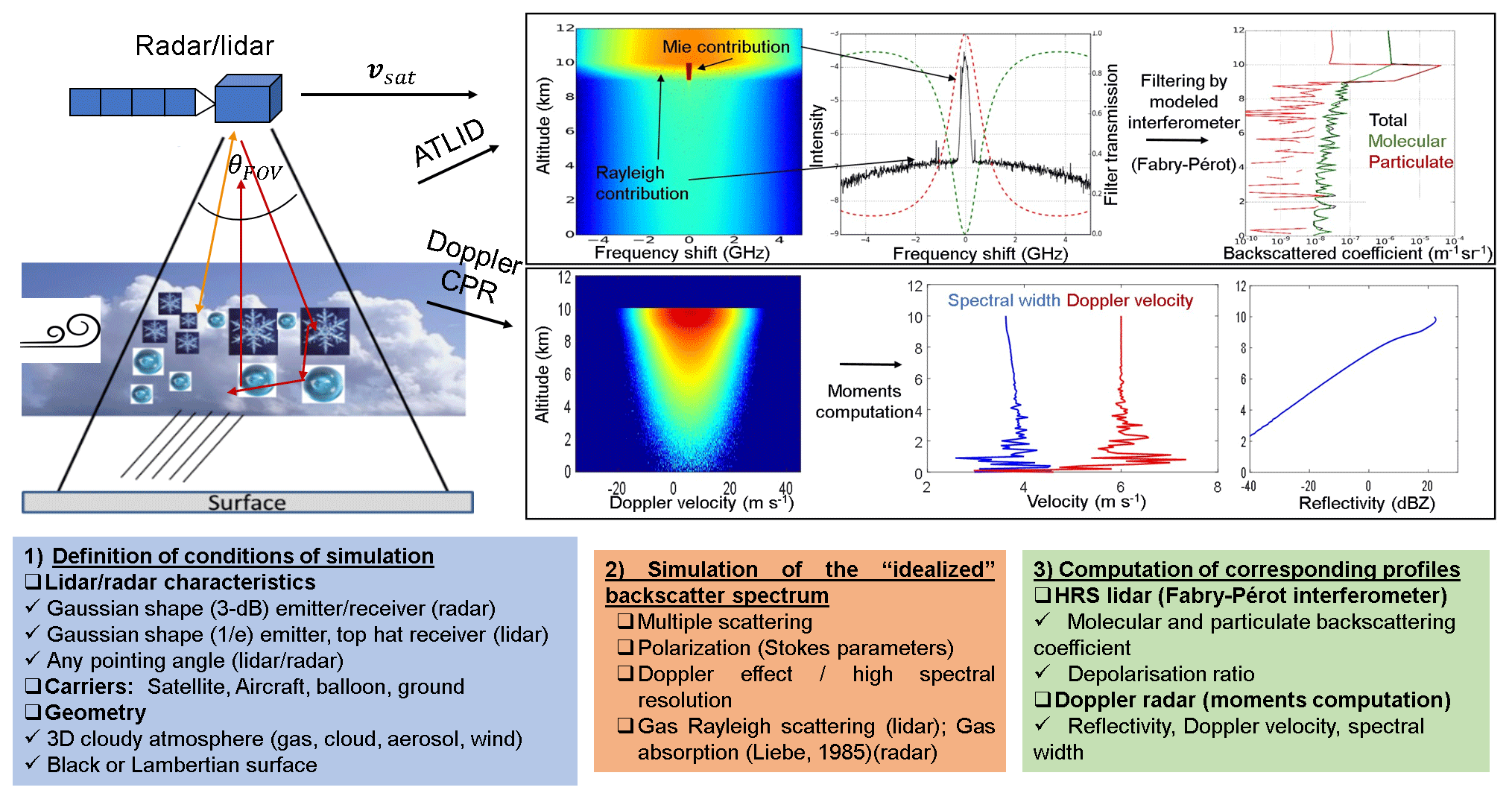
Figure 1Schematic presentation of the McRALI-FR simulator. Once the simulation conditions are defined (step 1), McRALI calculates the idealized backscatter spectrum (step 2). In the last step (step 3), using dedicated software, the desired quantity profiles are calculated. Note that cloud extinction between 9 and 10 km of altitude is set to 3 km−1 for both the lidar and radar simulation.
The simulation conditions (step 1 in Fig. 1) consists of setting the 3D optical and dynamical properties of the cloudy atmosphere, the surface, and main characteristics of the instrument (currently monostatic high-spectral-resolution lidar or a Doppler radar), which are its spatial position, its velocity, the viewing direction, the frequency and the polarization state of the emitted radiation, and the shape of the emitter and the receiver. If at least one of those parameters varies, the simulation has to be carried out once more even when 3D cloudy atmosphere properties remain unchanged. Computations are carried out and profiles of S(r,f) are stored in output files (step 2 in Fig. 1). Separate software uses the saved files to account for spectral and polarization characteristics of receivers and computes profiles of corresponding HSR lidar or Doppler radar signals (step 3 in Fig. 1), such as the particulate and molecular backscattering coefficient profiles for HSR lidar or reflectivity and Doppler velocity profiles for Doppler radar.
The next five subsections describe in detail how McRALI-FR accounts for the Doppler effect, the modeling of transmitter and receiver patterns, and the Lambertian ground surface and present two examples of the McRALI-FR configuration in order to simulate the HSR ATLID lidar and the Doppler CPR radar of the EarthCARE mission.
2.2 Modeling of idealized backscattered power spectrum profiles
McRALI-FR accounts for phenomena that lead to the frequency shift of the received photon. This is the Doppler effect, which is due to the motion of gas (negligible for radar application), aerosol (negligible for radar application), and cloud particles. We use the term “cloud particles” for precipitating hydrometeors as well.
When both the source and the receiver are moving, the Doppler effect can be expressed in a ground-based frame of reference as follows (see, e.g., Tipler and Mosca, 2008):
where fs and fr denote the frequencies; vs and vr are the velocity vectors; the source and receiver parameters are identified by the subscripts s and r, respectively; is the unit vector directed from the source to the receiver; c is the speed of electromagnetic waves; and a⋅b denotes the scalar product. If the absolute values |vs| and |vr| of the velocities are both small compared to the speed c, the series expansion of Eq. (4) takes the form
where the terms of the second order or higher than 1∕c are neglected.
In multiple-scattering conditions, Eq. (5) can be rewritten for the scattering order i as follows:
where n is the total number of scattering orders. The frequency f0 of an emitted photon and the vector of the satellite velocity belong to the set of input parameters for McRALI-FR.
In general, if a photon was scattered by particles n times, its frequency at the lidar–radar receiver is expressed as follows:
All terms of the second order or higher than 1∕c are neglected as above. The unit vector is directed from the satellite to the first scatterer; is directed from the last scatterer to the satellite. It should be noted that Eq. (7) is in agreement with Eq. (5) of the work by Battaglia and Tanelli (2011), wherein, at the scattering order i, the frequency shift Δfi can also be given by
where ki is the unit director vector defined between the scatterer i and i+1.
Figure 2 shows a schematic diagram of the frequency shift consideration at each interaction by using the local estimate method. A photon path of two scattering events within the lidar–radar FOV is represented in red. The velocity of the first and the second scatterer is v1 and v2, respectively. At the first and second scattering, the frequency shift is and , respectively. At each scattering event, McRALI-FR uses the local estimate method to compute the contribution to the detector. For example, at the second scattering event, the total frequency shift is computed as , where , with being the direction from the second scattering event to the detector (dotted blue line), which works with the local estimate method, and where , with vsat being the satellite velocity. The frequency shift due to satellite motion is deliberately ignored to simplify the scheme, but it is present in the codes. Computation of the McRALI-FR power spectrum can also be performed following the convention of the “Gaussian approach” proposed by Battaglia and Tanelli (2011).
Note that in the current version of McRALI-FR codes, the wind velocity can be set by the user or provided by large eddy simulation models at their grid scale. Sub-grid turbulence wind velocity is assumed to be homogeneous and isotropic; the turbulence velocity vector vturb is distributed according to a Gaussian probability density function (PDF) (see Wilczek et al., 2011, and references therein). The single-point velocity PDF has zero mean and the standard deviation σturb for all three coordinates of vturb. The multivariate normal distribution is generated using the Box–Muller method (see, e.g., Tong, 1990).
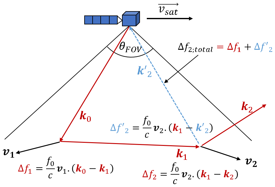
Figure 2Schematic diagram of the frequency shift consideration along the propagation of photons in scattering medium in the framework of the locate estimate method.
2.3 Modeling of transmitter and receiver pattern
The current version of the McRALI-FR codes only allows the monostatic configuration of transmitters and receivers of lidar or radar systems. Lidar–radar systems can be positioned at any altitude, allowing for ground-based, spaceborne, and airborne configurations with any viewing direction. The lidar transmitter is assumed to be a Gaussian laser beam with 1∕e angular half-width θlaser. For instance, a Gaussian laser beam pattern with 1∕e angular half-width θlaser is described by (Hogan, 2008)
The lidar receiver is assumed to be a top-hat telescope with a half-angle field of view θFOV, and its pattern can be described by (Hogan and Battaglia, 2008)
Radar transmitters and receivers are assumed to be Gaussian antennas with a 3 dB half-width θFOV. For instance, a Gaussian antenna pattern with 3 dB half-width θFOV is described by (Battaglia et al., 2010)
The lidar and radar transmitter and receiver pointing direction is defined by the zenith Θ0 and azimuthal ϕ0 angles. Direction cosines of the initial photon leaving the transmitter, calculated in the same way as Battaglia et al. (2006), are given by
where , , and with x1=tan η and x2=tan ξ. To reproduce the Gaussian pattern of Eqs. (9) and (11), η and ξ are Gaussian-distributed random numbers with zero mean and standard deviation equal to and , respectively. The multivariate normal distribution is generated using the Box–Muller method (see, e.g., Tong, 1990).
2.4 Modeling of a Lambertian surface
The current version of the McRALI-FR code uses the Lambertian surface model. The probability that a photon is scattered by the surface is defined by the albedo Λ. When Λ=0, i.e., the black surface model, it is assumed that all photons are absorbed by the surface. Otherwise, i.e., , the photon weight is multiplied by Λ. All photons scattered by the Lambertian surface are depolarized, i.e., have Stokes parameters of the form . The interaction of a photon with the surface is treated in the same way as scattering by a cloud or aerosol particle or the Rayleigh scattering (Cornet et al., 2010).
First, the new direction of a photon scattered by the surface is random and it is simulated according to the well-known algorithm (see, e.g., Mayer, 2009). The azimuth angle φ is chosen randomly between 0 and 2π.
As for the zenith angle θ, its cosine μ=cos(θ) is randomly drawn using the expression
where q1 and q2 are uniform random numbers between 0 and 1.
Secondly, the local estimate technique (Marchuk et al., 1980) is implemented to calculate at each scattering point the contribution of the photon in the direction of the sensor.
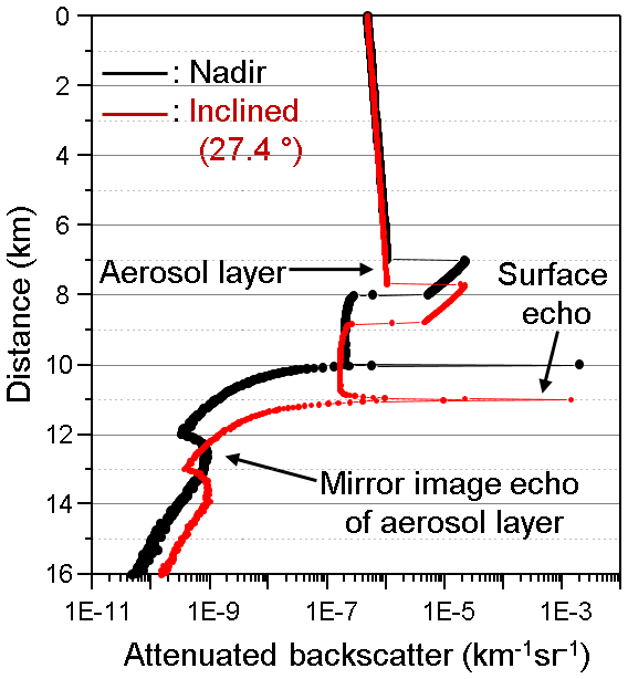
Figure 3Profiles of the attenuated backscatter (ATB) coefficient (black – nadir-looking, red – inclined at 24.7∘) as a function of the distance from the lidar position. The lidar altitude is 10 km.
Figure 3 shows as an example of the two lidar signals as a function of the distance from the lidar position for two viewing directions (nadir and inclined at 24.7∘, chosen so that the distance to the ground is 11 km). The lidar altitude is 10 km, the laser divergence is 0.0007, and the field of view of the receiver is 0.005 rad. An aerosol layer between altitudes of 2 and 3 km has an optical thickness of 0.15. The single-scattering albedo of 0.91888 and the phase function were computed with the refractive index and microphysical parameters of the coarse mode of desert dust, assuming that particles are spheroids with a distribution of the aspect ratio (Dubovik et al., 2006). The albedo of the Lambertian surface is set to 1.
For the nadir direction example, the layer at distances between 7 and 8 km that exhibits large values of the backscatter coefficient corresponds to the aerosol layer between 2 and 3 km in altitude. At a distance of 10 km, the very large value of the backscatter coefficient corresponds to the echo from the surface. Then, for distances larger than 10 km, the lidar signal drastically decreases. But for the distances from 12 to 13 km, another layer can be observed. That layer corresponds to a third and higher order of scattering. In this particular case, the triple scattering is of the type “surface–aerosol layer–surface”. It is also called the mirror image and refers to reflectivities measured by airborne or spaceborne radars at ranges beyond the range of the surface reflection (see, e.g., Battaglia et al., 2010). It should be underscored that the mirror image disappears when, during a simulation, one photon can undergo no more than two scatterings. The same behavior is observed for the case of the inclined viewing direction. The position of the aerosol layer, the surface echo, and the mirror image shifts in agreement with corresponding distances from the lidar.
The signal-to-noise ratio (SNR) of lidars is generally much lower than the SNR of radars. Thus, in practice it is impossible to observe a mirror image with a spaceborne lidar, contrary to a spaceborne radar. Results presented in Fig. 3 should be considered a numerical and theoretical exercise that demonstrates the McRALI capacities. The simulations were performed with a very high number of photon trajectories so that the numerical noise of the McRALI simulator is very low. Under these idealized simulation conditions, we show that McRALI is able to simulate lidar–radar systems with inclined sighting by taking into account the properties of the Lambertian surface, but also the mirror images (as it is seen in certain radar observations). It should be noted that to make the mirror image appear in this simulation, we have imposed a maximum surface albedo equal to 1.
2.5 Doppler radar CPR/EarthCARE configuration
2.5.1 Modeling gas absorption
At 94 GHz (3.2 mm, W band), the attenuation by atmospheric gas is mainly due to absorption of water vapor and oxygen (Liebe, 1985; Lenoble, 1993; Liou, 2002). The attenuation A (in dB km−1) by water vapor and oxygen in McRALI codes is computed from Liebe (1985) tabulations. Absorption coefficient σabs (in km−1) is given by σabs=0.2303 A. Absorption and scattering are treated separately in McRALI codes, as is done in 3DMCPOL (Fauchez et al., 2014), whereby absorption is considered by a photon weight wabs according to the Lambert–Beer law (Partain et al., 2000; Emde et al., 2011):
where ds′ is a path element of the photon path.
2.5.2 Doppler spectrum and its relation to reflectivity, Doppler velocity, and spectral width
The Doppler radar community uses the Doppler spectrum S(r,v), a power-weighted distribution of the radial velocities v in the velocity range dv of the scatterers (Doviak and Zrnić, 1984). McRALI-FR codes dedicated to Doppler radar simulations compute S(r,v) by using the first Stokes parameter I(r,f) and the Doppler formula . We follow the convention that the Doppler velocity is positive for motion away from the radar. The backscattering coefficient profile β(r) is then given by
The reflectivity Z(r) profile is computed using Eq. (3) and β(r). The Doppler velocity profile VDop(r) is defined as
and the Doppler velocity spectral width profile σDop(r) is obtained from
Figure 4 shows, as an example, a simulation of the Doppler power spectrum, the Doppler velocity, the Doppler velocity spectral width, and the reflectivity profiles for a CPR/EarthCARE-like radar for a homogenous iced cloud layer with fixed 6 m s−1 downdraft at all altitudes (see details of the conditions of the simulation in Table 1) with (σturb=0.5 ms−1) and without (σturb=0 ms−1) sub-grid turbulent wind. In a first step, McRALI-FR codes dedicated to Doppler radar simulations compute the idealized Doppler power spectrum density S(rv). The first Stokes parameter I(r,v) of the Doppler spectrums (with and without sub-grid turbulent wind) are shown in Fig. 4a and b, respectively. Then, in a second step, software computes the reflectivity, the Doppler velocity, and the Doppler velocity spectral width profiles with Eqs. (16), (17), and (18), respectively. Multiple-scattering (MS) and single-scattering (SS) Doppler velocity profiles are superimposed on the MS Doppler spectrum. MS and SS Doppler velocity values are constant within the cloud layer (between 9 and 10 km of altitude) and are equal to the “true” 6 ms−1 vertical velocity, whatever the wind turbulence value is. Due to multiple-scattering processes, the apparent Doppler velocity of 6 ms−1 can be observed between the cloud-base altitude and the ground, contrary to the SS apparent Doppler velocity, which appears only in the cloud layer.
In Fig. 4c the MS and SS Doppler velocity spectral width profiles are drawn. Under the SS approximation, the Doppler velocity spectral width σDop is given by (Kobayashi et al., 2003; Battaglia et al., 2013) , where σhydro is due to the spread of the terminal fall velocities of hydrometeors of different size, σshear is the broadening due to the vertical shear of vertical wind, σturb is the broadening of the vertical wind due to turbulent motions in the atmosphere, and σmotion is the spread caused by the coupling between the platform motion and the vertical wind shears of the horizontal winds. For a Gaussian circular antenna pattern, assuming zero fall velocities of hydrometeors and no wind shear, σDop is given by (Tanelli et al., 2002)
where vsat is the satellite velocity relative to the ground and θFOV is the Gaussian (3 dB) FOV half-angle.
Simulated SS Doppler velocity spectral widths without turbulence and with turbulence are close to 3.58 and 3.62 m s−1, respectively. Both computed values are very close to theory-predicted values. On the other hand, MS processes together with sub-grid turbulent wind are a source of broadening. For example, at 2 km under the cloud base, σDop=3.75 m s−1, which is larger than the SS value.
Vertical profiles of MS and SS reflectivity are shown in Fig. 4d. These profiles are not sensitive to the wind turbulence. MS processes are a source of enhancement of the reflectivity compared to the SS reflectivity and the apparent reflectivity that can be observed under the cloud layer.

Figure 4Estimated Doppler spectrum moments for a Doppler CPR/EarthCARE-like radar. (a) Doppler spectrum without wind turbulence. Doppler velocity profiles are superimposed (MS: dotted line, SS: cross). (b) Same as (a), but with wind turbulence. (c) Vertical profiles of MS (full lines) and SS (crosses) Doppler spectrum width with wind turbulence (red) and without wind turbulence (blue). (d) Vertical profiles of MS (full lines) and SS (crosses) reflectivity with wind turbulence (red) and without wind turbulence (blue). The altitude of the base of the iced homogeneous cloud layer (optical depth of 3) is 9 km. Its geometrical thickness is 1 km.
2.6 High-spectral-resolution (HSR) lidar ATLID/EarthCARE configuration
2.6.1 Modeling of the emitted laser energy spectrum
The laser transmitter of the ATLID instrument has spectral requirements with a spectral line width below 50 MHz (Hélière et al., 2017). In McRALI-FR codes, the frequency of the emitted radiation is drawn randomly according to a Gaussian law of average f0 with a 1∕e half-width MHz.
2.6.2 Modeling of thermal molecular velocity distribution
The current version of McRALI-FR codes assumes that each component of molecular velocity is distributed according to the Maxwell–Boltzmann density function with null mean and standard deviation a given by
where k is the Boltzmann's constant, T is the temperature, and m is the molecular mass of gas. The multivariate normal distribution is generated using the Box–Muller method. As a next step, we plan to take into account spontaneous Rayleigh–Brillouin scattering.
2.6.3 Relation of the HSR spectrum to molecular and particulate backscattering coefficient: modeling of a Fabry–Pérot interferometer
One of the important features of HSR lidars is the possibility to retrieve profiles of particle extinction and the backscattering coefficient without the need for additional information on the lidar ratio (Shipley et al., 1983; Ansmann et al., 2007, and references therein). HSR technology relies on the principle of measuring the Doppler frequency shift resulting from the scattering of photons by molecules (referred to as molecular scattering or Rayleigh scattering) and by particles (referred to as particulate scattering or Mie scattering). The characteristic shape of the HSR spectrum depends on both these two scattering processes: a broad spectrum of low intensity for molecule scattering and a narrow peak of large intensity for particle scattering.
The spectral width of the particle peak will be determined by the spectral width of the laser pulse itself along with any turbulence present in the sampling volume. The spectral width of the ATLID laser will be on the order of 50 MHz so that the laser line width will be the dominant factor. Thus, the molecular backscatter will be much broader than the particulate-scattering return. This is due to the fact that atmospheric molecules have a large thermal velocity. Assuming a Gaussian molecular thermal velocity distribution with a half-width at 1∕e of the maximum, molecular broadening γm can be written (Bruneau and Pelon, 2003) as
If T=230 K, then γm is of the order of 2 GHz, which is about 40 times larger than the laser line width. Thus, using interferometers (such as the Fabry–Pérot (FP) interferometer equipping the ATLID/EarthCARE lidar) and appropriate signal processing (Hélière et al., 2017), the molecular and particulate contributions of the lidar backscattered signal can be separated. Then particulate and molecular backscattering coefficient profiles (attenuated or apparent attenuated backscattering coefficient or simply attenuated backscatter, also denoted as ATB) can be separately determined. In this study, we suppose that the FP interferometer has the following parameters. The free spectral range is 7.5 GHz, the finesse is 10, and the FP is centered at the wavelength 355 nm. The cross-talk effects were taken into account according to the work by Shipley et al. (1983). The coefficients of the cross-talk correction were computed using an Airy function (see, e.g., Vallée and Soares, 2004), which describes the FP transmission spectrum, assuming a Gaussian molecular thermal velocity distribution with a half-width at 1∕e of the maximum γm (Eq. 21). This method determines four calibration coefficients corresponding to the fraction of cloud–aerosol backscatter in the molecular and particulate channels (Cam and Caa, respectively), as well as the fraction of molecular backscatter in the molecular and particulate channels (Cmm and Cma, respectively). The calculation method of these coefficients is described in detail in Shipley et al. (1983). As an indication, for the present study in the ATLID/EarthCARE lidar configuration, these coefficients have the following values: Cmm=0.543, Cma=0.457, Caa=0.998, and Cam=0.002. Note that the cross-talk coefficients used in this paper assume ideal behavior of the ATLID FP interferometer. In practice, the Airy function will be “blurred” due to the effects of nonideal collimation of the beam, frequency jitter, surface roughness, and so on. All these factors combine to decrease the peak transmission and lower the full-width at half-maximum (see the Fig. 9 in Pereira do Carmo et al., 2019). It is important to keep in mind that all the calculations shown in this paper are merely “EarthCARE-like” but with an idealized modeled FP interferometer.
Figure 5 shows particulate and molecular ATB profiles for an ATLID/EarthCARE-like lidar. We consider in this example an ice cloud corresponding to a homogenous layer with an optical depth 3 between 9 and 10 km in altitude (see details of the simulation conditions in Sect. 3.1). In the first step, McRALI-FR codes, dedicated to HSR lidar simulations, compute the HSR spectrum S(rf). The first Stokes parameter I(r,f) of the MS HSR spectrum is shown in Fig. 5a. The peak of intensity (in red) centered at 0 GHz between 9 and 10 km of altitude corresponds to the position of the cloud. It is the contribution of the cloud particles (the so-called “Mie contribution”). This spectrum is also characterized by the molecular contribution (Rayleigh contribution). The intensity of the spectrum below the cloud is lower than the intensity of the spectrum above the cloud due to particulate extinction. In Fig. 5b, the MS (computed with McRALI-FR) and SS (computed from SS theory) vertical profiles of spectral width are represented. We note very good agreement between the SS theoretical and MS simulated values at both the cloudy and molecular levels. This suggests that MS effects have very little impact on spectral width. Then, in a second step, a simulated FP interferometer separates the particulate contribution from the molecular contribution and provides the vertical profiles of particulate and molecular ATB as shown in Fig. 5c. The total ATB calculated directly from the spectrum, SS molecular, and SS particulate backscatter profiles is also represented. Above the cloud, particulate ATB is not strictly zero and molecular ATB is not strictly equal to total ATB because of the FP remaining cross-talk effects (see above). In the cloudy part between 9 and 10 km of altitude, the molecular and particulate ATB logically decrease exponentially with depth. The SS backscatter profiles decrease faster with depth than the MS backscatter profiles, revealing that MS effects on ATB are not negligible. Under the cloud, molecular ATB is almost equal to total ATB. It is likely worth pointing out the quasi-exponential decay of the below-cloud molecular return towards single-scattering levels. This result is consistent with the cases shown by Donovan (2016). Particulate ATB is almost zero. Some nonzero values exist due to FP cross-talk effects but also due to Monte Carlo noise and MS processes.
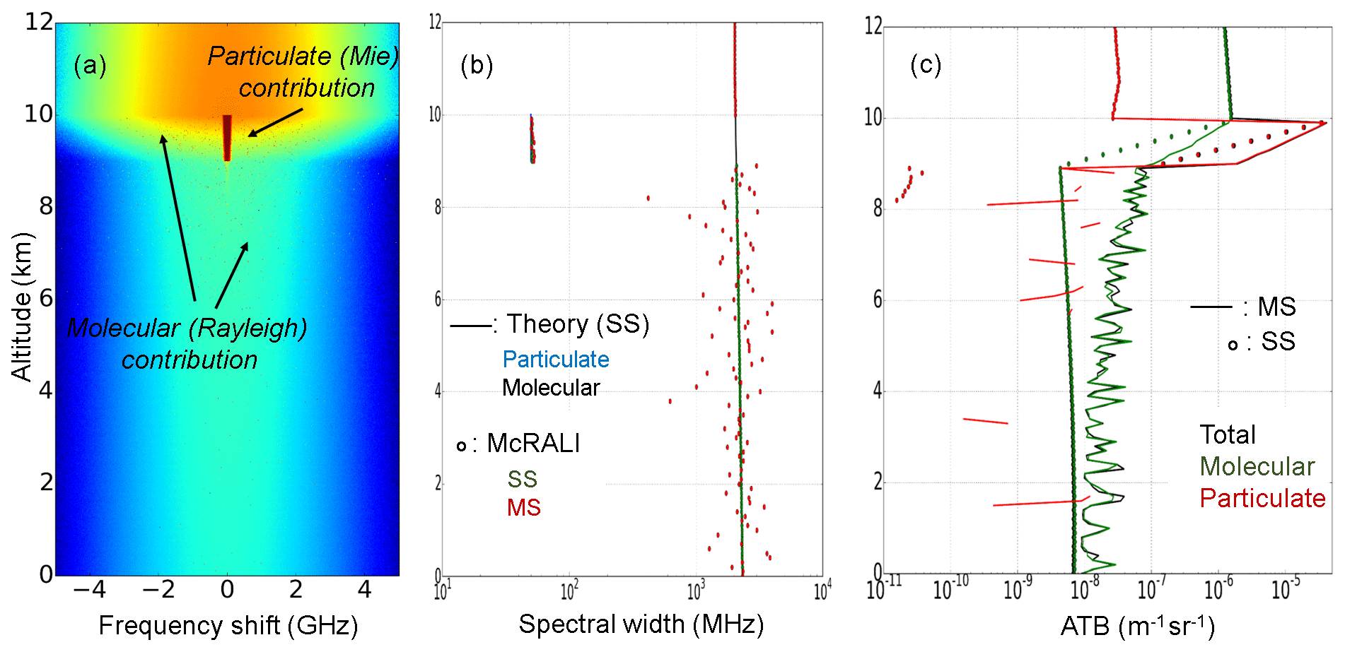
Figure 5(a) Vertical profile of MS HSR spectrum for an ATLID-like lidar. (b) Spectral width profiles. SS and MS spectral width profiles computed by McRALI (circle) are in green and red, respectively. Theoretical SS molecular and SS particulate width profiles (full line) are in black and blue, respectively. (c) Vertical profiles of the MS (line) and SS (circle) backscattered coefficient (ATB). Total, molecular, and particulate signals are in black, green, and red, respectively. The altitude of the base of the iced homogeneous cloud layer (optical depth of 3) is 9 km. Its geometrical depth is 1 km.
The objectives of this section are to investigate the effects of a cloudy atmosphere having 3D spatial heterogeneities under a multiple-scattering regime on HSR lidar and Doppler data by using McRALI-FR simulators. One of the simplest shapes of heterogeneous cloud to study this kind of effects is the idealized “step” cloud defined in the international Intercomparison of 3D Radiation Codes (I3RC) phase 1 (Cahalan et al., 2005). The main interest is to model behavior in the vicinity of the single isolated jump in optical depth. With this in mind, we prefer to use an even more simplistic cloud model, the box cloud, described in the following paragraph. A detailed statistical analysis at different averaging scales of representative fine-structure 3D cloud field effects on lidar and radar observables is beyond the scope of this paper and will be investigated in a future work.
3.1 Conditions of simulation and definition of the box cloud
The box-cloud base altitude is 9 km, its geometrical thickness is 1 km, and its x-horizontal and y-horizontal extension is 2 km and infinite, respectively. Temperature and pressure vertical profiles assume 1976 US standard atmosphere models. Optical cloud properties are characterized by the extinction coefficient set to 0.1, 1.0, and 3 km−1.
Figure 6 shows a representation of two specific positions of a spaceborne lidar–radar system relative to the idealized box cloud. Cloud optical properties are spatially homogeneous within the box cloud. When the lidar–radar system is just above the cloud edge, the NUBF effect can be significant, whereas it is null when the system is completely over the cloud. Table 1 summarizes the conditions of McRALI-FR simulations for data from the HSR ATLID lidar and Doppler CPR radar of the EarthCARE mission when the heterogeneous box cloud is considered.
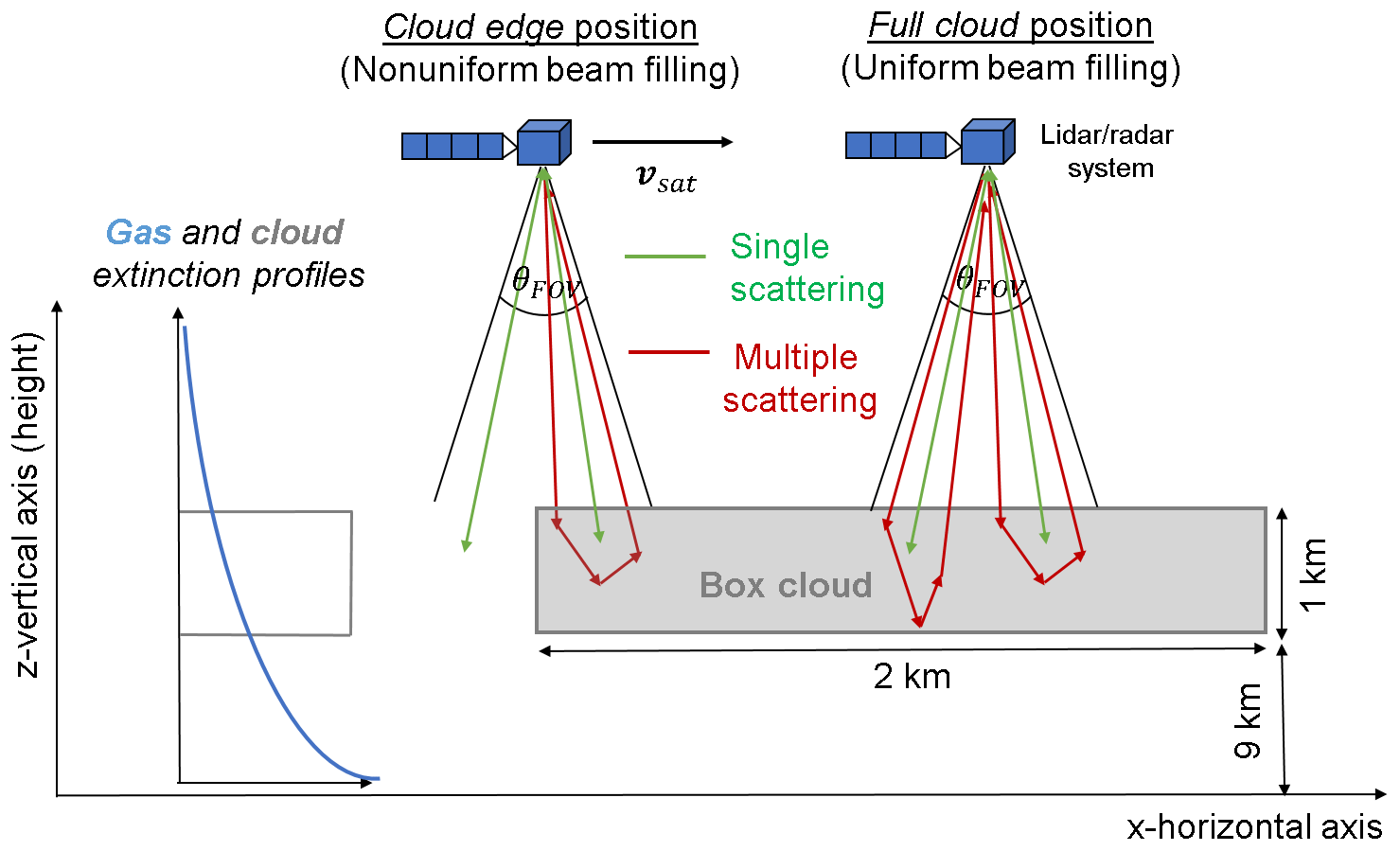
Figure 6Schematic representation of two specific positions of a spaceborne lidar–radar system relative to the idealized box cloud. The box-cloud base altitude is 9 km, its geometrical thickness is 1 km, and its x-horizontal and y-horizontal extension is 2 km and infinite, respectively. The cloud vertical extinction profile is constant. In the two positions, single- and multiple-scattering photon path examples are represented by green and red arrows, respectively.
At a wavelength of 355 nm (lidar configuration), gas scattering properties are based on Hansen and Travis (1974). Gas Doppler broadening is computed assuming a Maxwell–Boltzmann distribution as presented in Sect. 2.4.1. The scattering matrix was computed for a gamma size distribution of ice crystals having an effective diameter of 50 µm and the aspect ratio of 0.2. The refractive index value was ; the surface of particles was assumed to be rough (Yang and Liou, 1996). Optical characteristics were computed using the improved geometric optics method (IGOM) (Yang and Liou, 1996). The asymmetry parameter is g=0.73, which is in agreement with experimental data for cirrus clouds (Gayet, 2004; Shcherbakov et al., 2006). Single-scattering albedo is set to 1.0.
At 94 Ghz (radar configuration), we assumed a Henyey–Greenstein phase function with an asymmetry parameter g=0.6. Single-scattering albedo is set to 0.98. These last two values are taken from Battaglia and Tanelli (2011) for a scenario involving a deep convective core with graupel. Wind vertical velocity (downdraft) is set to 6 ms−1. We assume no wind turbulence nor particle sedimentation velocity. For a cloud layer at an altitude of around 9 km, the pressure, temperature, and relative humidity can be set to 308 hPa, 229.7 K, and 100 %, respectively (1976 US standard atmosphere); then gas absorption km−1. We assumed that this value is small enough to neglect the gas absorption for the simulations carried out in this work.
Spacecraft velocity and altitude are set to vsat=7.2 km s−1 and 393 km, respectively. The lidar–radar system pointing angle is set to 0∘. The lidar transmitter is assumed to be a Gaussian laser beam with 1∕e angular half-width θ=22.5 µrad. The lidar receiver is assumed to be a top-hat telescope with a half-angle field of view θFOV=32.5 µrad, which represents a ground beam footprint of around 30 m. Radar transmitters and receivers are assumed to be Gaussian antennas with a 3 dB half-width ∘, which represents a ground beam footprint of around 660 m.
McRALI-FR code simulates the multiple-scattering and single-scattering idealized HSR and Doppler spectrum for lidar and radar configurations, respectively. Lidar spectra are computed for five positions (x-horizontal ground-projected distance) relative to the box-cloud edge. Lidar position values are , and 8.6 m. Indeed, the ratio (we also talk about cloud coverage) of the cloudy part inside the ATLID lidar FOV divided by the full lidar footprint area at the altitude of 10 km is 10 %, 30 %, 50 %, 70 %, and 90 %, respectively. Then, software computes apparent molecular and particulate backscattering coefficient profiles, assuming that the ATLID/EarthCARE lidar is equipped with FP interferometers (see Sect. 2.5.3). For the radar configuration, simulations are carried out every 100 m; Doppler spectra are computed for position values fixed at , −250, 0, 250, and 500 m. Then, software computes reflectivity, Doppler velocity, and Doppler velocity spectrum width profiles with the help of Eqs. (16), (17), and (18).
Table 1Description of the simulation conditions presented in this work. This table summarizes the characteristics of the ATLID/EarthCARE-type lidar and the CPR/EarthCARE-type radar as well as properties of a cloudy atmosphere and quantities computed by McRALI-FR codes.
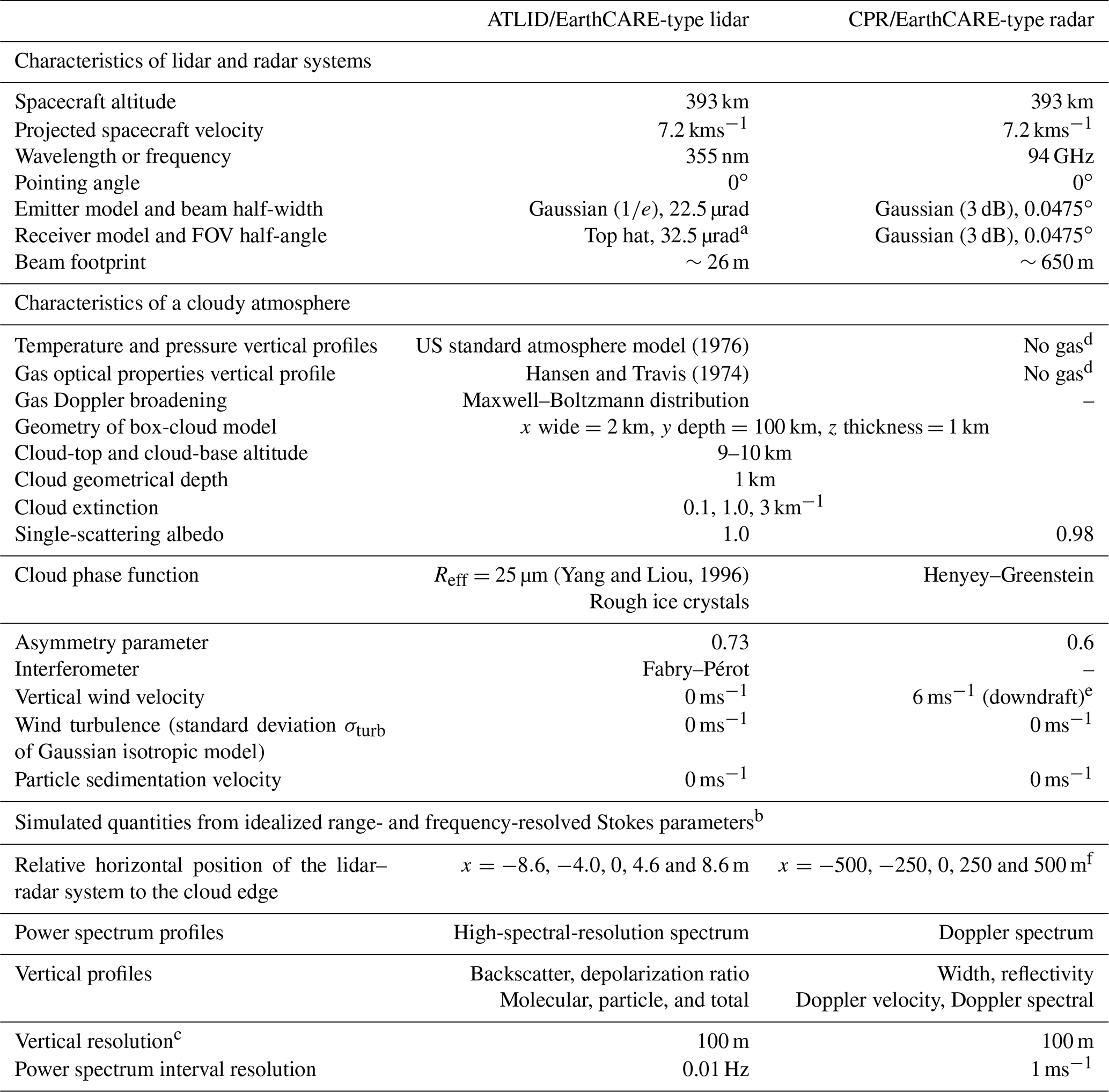
a Other simulations are performed with an FOV half-angle of 325 µrad. b Idealized means that receiver noise, along-track integration, and Nyquist folding are ignored. c ATLID and CPR vertical resolution is 100 m from −1 to 20 km in height. d Gas absorption (Liebe, 1985) can be taken into account. e A specific case with a two-layer cloud with 6 and −6 ms−1 vertical wind velocity in the top layer and bottom layer, respectively, is also studied. f For radar configurations, simulations are also carried out every 100 m according to the horizontal distance.
3.2 CPR/EarthCARE configuration
3.2.1 NUBF effects on Doppler radar data: Doppler spectrum and reflectivities
Figure 7a–e show vertical profiles of MS radar Doppler spectra density in the CPR/EarthCARE configuration corresponding to the five positions of the satellite relative to the edge of the box cloud with optical depth set to 3. Regardless of the satellite position, Doppler spectra correspond to negative Doppler velocity values. This is consistent with the convention that the Doppler velocity is positive for motion away from the radar. As the satellite approaches the edge of the cloud and carries on, the NUBF effect decreases. Indeed, the Doppler spectrum becomes more and more symmetrical. The asymmetric shape of the Doppler spectrum is due to zero values beyond a critical value of Doppler velocity vcrit. As an example, ms−1 in Fig. 7a. The explanation of the vcrit value is purely geometric. Doppler broadening is dominated by Doppler fading due to satellite motion. Under the SS approximation, neglecting wind velocity, the Doppler shift is given by , with . Assuming vsat with an x-horizontal positive component, k0, in the (z–x) vertical plan and with kx as the x-horizontal component, then . Assuming that satellite is at the x-horizontal d distance to the box-cloud edge and at the z-vertical D distance above the cloud, with a vertical (downdraft) wind velocity vwind fixed at 6 ms−1, then . For , , x=0, x=250, and x=500 m, , , vcrit=6, vcrit=10.7, and vcrit=15.4 m s−1, respectively. These values are very close to those estimated from the five respective power spectra in Fig. 7.

Figure 7Vertical profiles of MS radar Doppler spectra (logarithm of the spectral density; in m−1 sr−1 (m s in the CPR/EarthCARE configuration corresponding to the five positions m (a), m (b), x=0 m (c), m (d), and m (e) of the satellite relative to the edge of the box cloud. SS (black line) and MS (black dotted line) vertical profiles of Doppler velocity are superimposed. The vertical wind velocity profile (downdraft) fixed at wwind=6 m s−1 during our simulation is also drawn (black dotted line). (e) The five reflectivity (in dBZ) profiles (MS: full lines, SS: dotted lines) corresponding to the five positions ( in blue, in red, x=0 m in brown, x=250 m in green, and x=500 m in magenta) relative to the edge of the box cloud. Cloud optical depth is 3.
Figure 7f also shows the five reflectivity profiles corresponding to the five positions of the satellite relative to the edge of the box cloud. MS reflectivity profiles are larger than SS reflectivity profiles because MS processes logically increase the reflectivity value. We can also see MS effects on the apparent reflectivity that is non-null under the cloud layer, contrary to the SS apparent reflectivity. At the same time, as the satellite approaches the edge of the cloud and keeps moving forward, SS and MS apparent reflectivity profile values increase due to the fact that the NUBF effect decreases. Many studies have focused on the NUBF effect on rain fields retrieved by radar from space (Amayenc et al., 1993; Testud et al., 1996; Durden et al., 1998; Iguchi et al., 2009). Iguchi et al. (2000) showed that the NUBF effect could be accounted for by a factor determined from horizontal variation of the attenuation coefficient. Our simulations are coherent with the literature. A detailed investigation of the NUBF effect on reflectivity profiles for spaceborne cloud radar will be carried out in a later work.
3.2.2 NUBF effects on Doppler velocity and Doppler spectrum width
Figure 7 shows the SS and MS vertical profiles of Doppler velocity superimposed on the five power spectra for the five positions of the satellite relative to the box-cloud edge: , −250, 0, 250, and 500 m. Since each power spectrum has no value beyond the vcrit velocity, which is due to the NUBF effect, it is obvious that the profile of the apparent Doppler velocity is different from the profile of the vertical wind velocity fixed at 6 ms−1. Figure 8 shows the MS and SS apparent Doppler velocity and Doppler spectrum width computed every 100 m along the horizontal axis. These quantities are estimated at different altitudes (cloud top, middle, and base) and are plotted as a function of the satellite distance to the box-cloud left edge. Differences between apparent Doppler velocities are in general small (around 1 m s−1) whatever the altitude is, and differences between MS and SS Doppler velocities are also small, no larger than 1 m s−1 at the bottom of the cloud. The same conclusions can be drawn for the Doppler spectrum width at which differences are no larger than 0.3 m s−1. This implies that MS processes do not play an important role in the estimation of the apparent Doppler velocity or in the estimation of apparent spectrum width (for the specific conditions of simulation with the box cloud) compared to the NUBF effect. The NUBF Doppler velocity bias between apparent Doppler velocity and “true” vertical wind velocity fixed at 6 m s−1 is around −10, −5, −3, −2, and −1 ms−1 at , −250, 0, 250, 500 m, respectively.
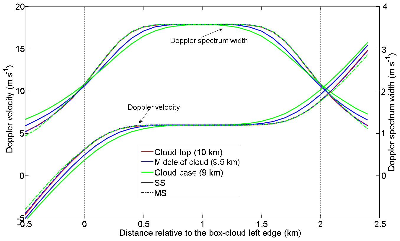
Figure 8MS (full lines) and SS (dotted line) apparent Doppler velocity and Doppler spectrum width as a function of the distance of the satellite relative to the box-cloud left edge. Values are computed at cloud top (10 km of altitude, in red), middle (9.5 km of altitude, in blue), and base (9 km of altitude, in green). Optical thickness of the box cloud is 3. Simulations are done every 100 m.
In general the NUBF bias of Doppler velocity can be expressed as a function of the distribution of the radar reflectivity (Tanelli et al., 2002). An estimate of the NUBF bias of Doppler velocity can be obtained by considering the difference between the Doppler velocity computed with a satellite velocity (i.e., vsat=7.2 kms−1) and the Doppler velocity computed with a satellite velocity set to 0 m s−1 (Battaglia et al., 2018). Sy et al. (2014) showed that the NUBF bias of Doppler velocity is correlated with the horizontal gradient of reflectivity and demonstrated that the theoretical proportional coefficient α value is bounded between 0.165 and 0.219 m s−1 (dBZ km. Kollias et al. (2014) estimated this proportional coefficient value close to α=0.23 m s−1 (dBZ km for along-track horizontal integration of 500 m (i.e., Doppler CPR/EarthCARE resolution) and for all their available simulations performed with a cirrus cloud and a precipitation system. Figure 9 shows the Doppler velocity NUBF bias as a function of the horizontal reflectivity gradient for a horizontal integration of 500 m at four positions relative to the box-cloud edge (−200, 100, 0, and 100 m). Computations are carried out for different optical depths of the box cloud of 0.1, 1, and 3. We note that the α value is between 0.14 and 0.16 m s−1 (dBZ km and is almost independent of the position of the satellite relative to the box-cloud edge. If the satellite position is just above the cloud edge, the proportional coefficient value is close to 0.15 m s−1 (dBZ km, a value close to that obtained by Sy et al. (2014).
3.2.3 Effects of vertically heterogeneous wind velocity on Doppler velocity
A first study of the effects of multiple scattering on the Doppler velocity vertical profile in the case of vertically heterogeneous wind velocity is carried out for a very specific case in the CPR/EarthCARE configuration. Indeed, for a homogeneous cloud layer with a base altitude of 9 km and with a geometrical thickness of 1 km, the vertical velocity is set to 6 m s−1 (downdraft) and −6 m s−1 (updraft) in the upper and lower part of the cloud layer, respectively. Figure 10 shows vertical profiles of the MS radar Doppler spectrum and the MS and SS Doppler velocity profiles computed with McRALI-FR. The measured Doppler velocity under the SS regime (black dotted line in Fig. 10) is equal to 6 m s−1 (−6 m s−1) in the upper (lower) part of the cloud, and the SS Doppler velocity can be used as the reference of the true velocity. In the upper part of the cloud, the measured MS Doppler velocity is 6 m s−1, which equals the true velocity. In the lower part of the cloud, the measured MS Doppler velocity is biased by multiple-scattering processes with a value not smaller than −3 m s−1, contrary to the true velocity of −6 m s−1 in this cloudy part. For altitudes lower than 7 km, we can also note that multiple-scattering processes can lead to a Doppler velocity lower than −6 m s−1.
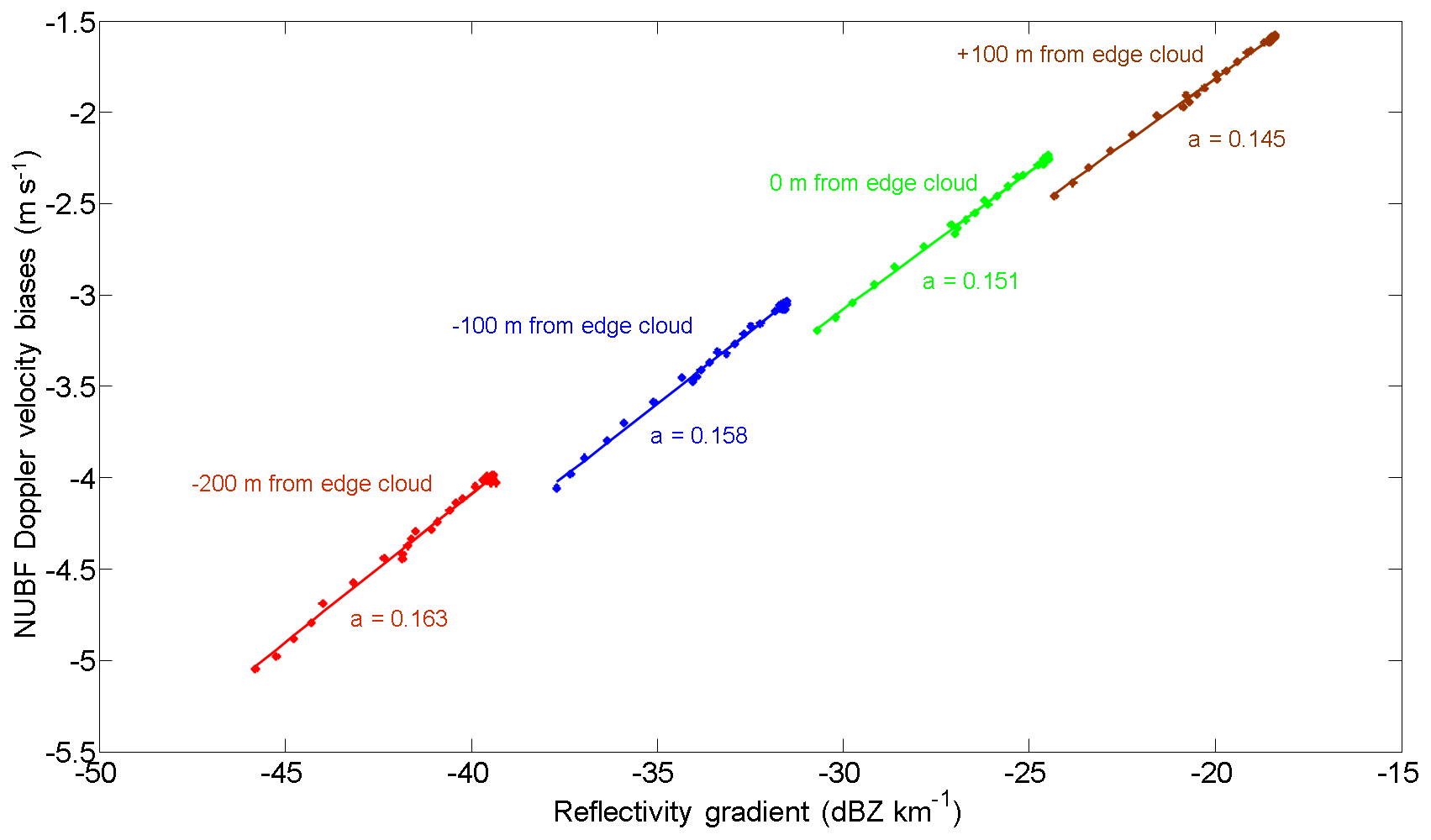
Figure 9NUBF velocity bias as a function of the horizontal reflectivity gradient for a horizontal integration of 500 m, estimated for four positions relative to the box-cloud edge: −200 m (red), −100 m (blue), 0 m (green), and +100 m (brown). Optical depths of the box cloud are 0.1, 1, and 3. Vertical (downdraft) velocity is set to 6 m s−1. The proportional coefficient value α (in m s−1 (dBZ km between NUBF velocity bias and horizontal reflectivity gradient is also given.
3.3 ATLID/EarthCARE configuration
3.3.1 NUBF effects on the HSR lidar data
In order to investigate the NUBF effects on HSR lidar observables under MS regimes we firstly compare simulation results carried out with the box cloud (full 3D simulation) and an optical depth equal to 3 (hereafter called 3D cloud) to simulations performed with the plane-parallel and homogeneous cloud model (hereafter called PP cloud) as well as with the independent column approximation (or independent pixel approximation) cloud model (hereafter called ICA cloud). PP theory and the ICA assumption are commonly used to assess the radiative effects of inhomogeneous cloud when cloud unresolved variability and net horizontal fluxes, respectively, are ignored (Marshak and Davis, 2005). For the specific case of the satellite position relative to the box-cloud edge m (see Fig. 11a), and the cloud coverage α inside the lidar receiver FOV is 30 % (see Sect. 3.1). As cloud optical depth (COD) is set to 3, this implies that mean COD weighted by the cloud coverage inside the lidar footprint is 0.9, the assigned value for the optical depth of the PP cloud (Fig. 11b). In other words, the PP profile can be considered a profile computed for a homogeneous cloud with optical depth equal to the mean optical depth of the cloudy part weighted by the cloud cover of the 3D cloud. The ICA simulation is carried out by averaging 30 % of a simulation with a homogeneous cloud with COD of 3 % and 70 % of a simulation in a clear-sky atmosphere (Fig. 11c). In other words, ICA profiles can be considered a profiles averaged over columns (two columns in this case) weighted by the cloud coverage.
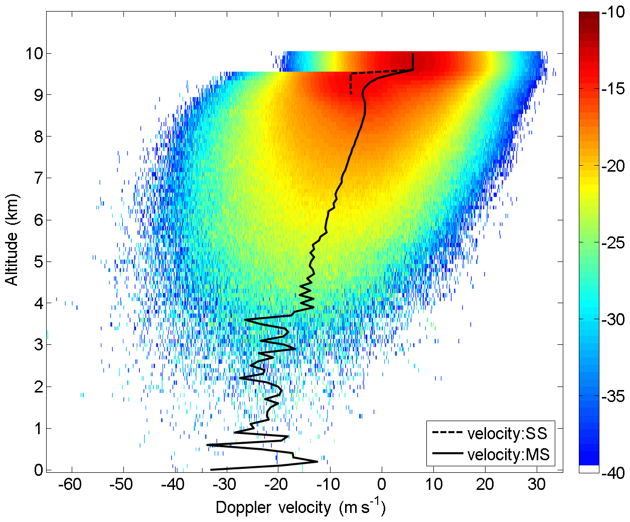
Figure 10Vertical profiles of an MS radar Doppler spectrum (logarithm of the spectra density; in m−1 sr−1 (m s in the CPR/EarthCARE configuration simulated by McRALI-FR. The MS Doppler velocity (black line) and SS (black dotted line) vertical profiles of Doppler velocity are superimposed. The homogeneous cloud layer base altitude is 9 km; its geometrical thickness is 1 km. The vertical velocity is set to 6 m s−1 (downdraft) and −6 m s−1 (updraft) in the upper and lower part of the cloud layer, respectively. Optical depth is 3.

Figure 11Conceptual representation of cloud models used for the HSR lidar simulations: (a) box-cloud model (3D), (b) plane-parallel and homogeneous (PP) model, and (c) independent column approximation (ICA) cloud. The purple circles represent the lidar footprint location for the simulations.
Figure 12 shows the HSR spectra simulated by McRALI-FR for the three cloud models at four altitude levels: above the cloud (12 km, Fig. 12a), at cloud top (9.8 km, Fig. 12b) and base (9.2 km, Fig. 12c), and below the cloud (8.5 km, Fig. 12d). In the clear-sky region above the cloud (Fig. 12a), the three frequency spectra line up very well, as expected, because the lidar laser beam has not yet been scattered by the cloud. A similar feature is observed at cloud top (Fig. 12b), whereas a few spikes can be seen in the molecular broad spectrum. Deeper in the cloud (Fig. 12c) and below (Fig. 12d), spikes are more numerous with higher intensity. These spikes are simulation artifacts. They are caused by specific events of multiple scattering, namely by cases when forward scattering is involved during a photon random path. For example, the photons can first be scattered by air molecules, inducing a large frequency shift, then by cloud particles, inducing a large contribution due to the highly forward-peaked phase function. The scattering phase function of ice particles spans about 6 orders of magnitude. Thus, the forward-scattered photons have a weight that is several orders of magnitude larger than those scattered in other directions. At the same time, such cases occur rarely. Consequently, we should carry out simulations with an unrealistic number of photons emitted by the lidar to smooth spikes, which is not possible. Spikes are not observed in simulations under the single-scattering regime (not shown here).
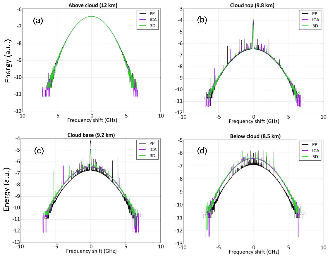
Figure 12Normalized HSR power spectra (a) above the cloud (12 km of altitude), (b) at cloud top (9.8 km of altitude), (c) at cloud base (9.2 km of altitude), and (d) below the cloud (at 8.5 km of altitude). Black lines represent simulations using the PP cloud model, purple lines the ICA cloud model, and green lines the 3D box-cloud model.
One can clearly see that the intensity of the central Mie (particulate) peak computed by ICA and 3D is lower than the one computed by the PP simulation. The opposite behavior is observed concerning the Rayleigh (molecular) scattering region: the broad and low-intensity spectra for ICA and 3D simulations show larger values (in intensity) compared to the PP simulation and for the full range of frequency shift. The same observation can be made below the cloud.
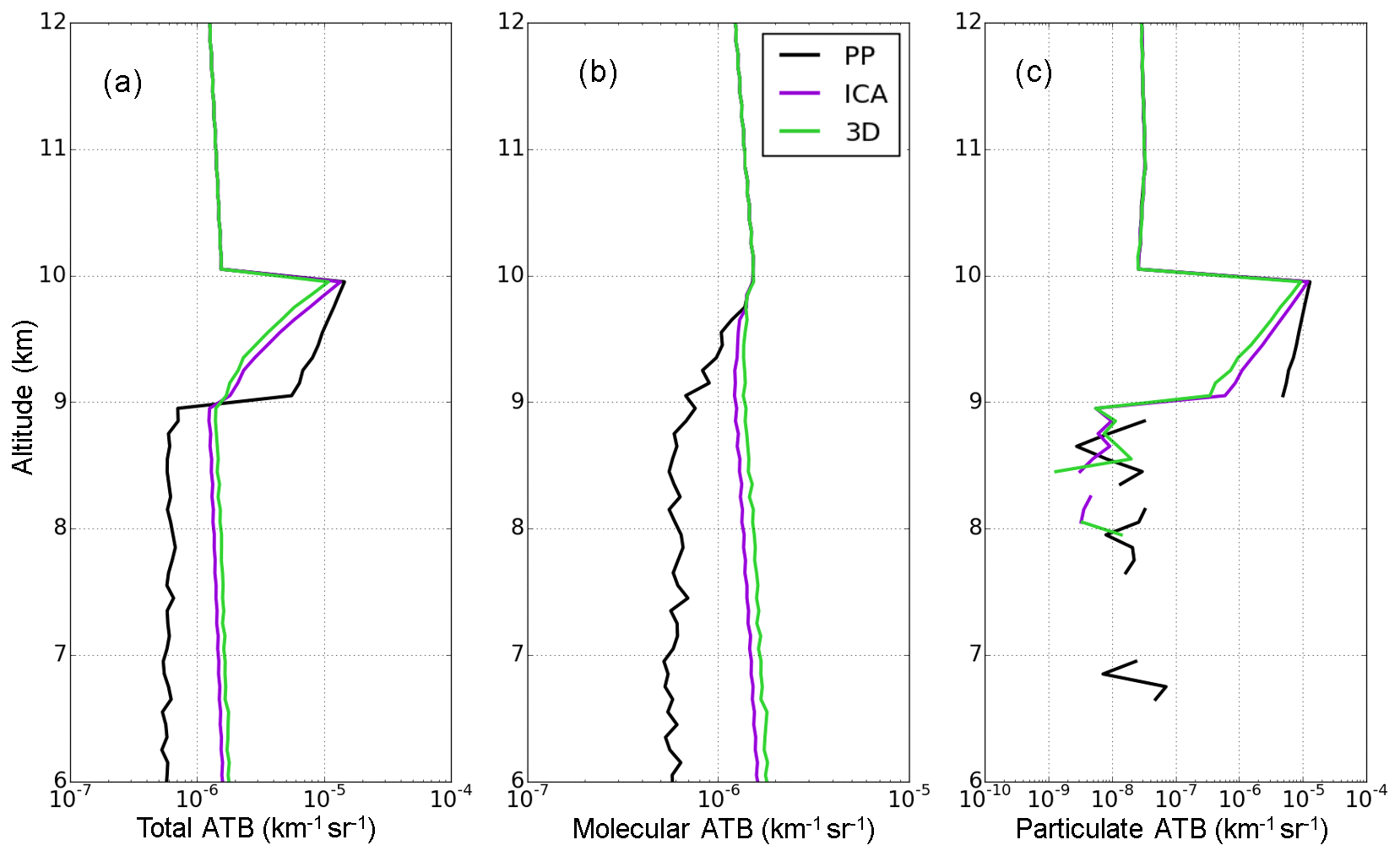
Figure 13Vertical profiles of (a) total, (b) molecular, and (c) particulate ATB simulated by McRALI. The cloud is located between 9 and 10 km. Black lines represent simulations using the PP cloud model, purple lines the ICA cloud model, and green lines the 3D box-cloud model.
In order to obtain the molecular and particulate ATB vertical profiles for the three cloud models (Fig. 13b and c), the HSR spectra are filtered by a modeled Fabry–Pérot interferometer (see Sect. 2.5.3 for the filtering parameters) at each altitude level. The ATB vertical profiles (Fig. 13a) exhibit features observed in HSR spectra more clearly: once the cloud is reached (i.e., below 10 km), the three cloud models give very different total ATB. Higher values are observed in clouds for the PP model compared to ICA and 3D cloud models, whereas the opposite is observed below the cloud. This feature shows that PP cloud representation can lead to large discrepancies and is suitable to account for 3D cloud structure. In contrast, ICA cloud models give results rather close to 3D cloud models. In Fig. 13b and c the PP cloud shows the most significant differences, with PP particulate ATB in the cloud larger than ICA and 3D particulate ATB and a PP molecular ATB that is smaller. To a lesser extent, ICA and 3D computations also show differences with 3D total and 3D particulate ATB smaller than the ICA computation. This difference is the opposite for molecular ATB.
In order to quantify the differences coming from the cloud models, PP, ICA, and 3D biases have been computed. These biases, well described in Davis and Polonsky (2005), were first defined in the radiance framework by Cahalan et al. (1994) and were adapted to a lidar signal framework by Alkasem et al. (2017). The 3D bias on ATB (i.e., ΔATB3D) is the sum of the PP bias (i.e., ΔATBPP) and the ICA bias (i.e., ΔATBICA) defined as
where ATBICA, ATBPP, and ATB3D are ATB computed by McRALI with the ICA, PP, and 3D cloud models, respectively. The relative biases are also computed and correspond to the biases divided by the reference ATB3D. In Appendix B, it is shown that the PP bias of molecular ATB and particulate ATB is always negative and positive, respectively. It is also shown that the larger multiple scattering, the smaller the PP particulate bias. Note that the PP bias of total ATB is positive but becomes negative with increasing cloud optical depth (Alkasem et al., 2017).

Figure 14Vertical profiles of biases on (a) total, (b) molecular, and (c) particulate ATB and vertical profiles of relative biases on (d) total, (e) molecular, and (f) particulate ATB. Black lines represent simulations using the PP cloud model, purple lines the ICA cloud model, and green lines the 3D box-cloud model.
Figure 14 shows that the PP biases are the largest on total ATB as well as the molecular and particulate components. Indeed, they reach 250 %, −60 %, and 1200 % for total, molecular, and particulate ATB, respectively. The ICA biases present lower values (around 25 %, −10 %, and less than 100 % for total, molecular, and particulate ATB, respectively). These results thus show that 3D biases are mainly due to PP biases.
Based on the three cloud models, further simulations have been carried out with varying the cloud coverage inside the lidar FOV from 10 % to 90 % in order to evaluate the impact of cloud coverage on HSR lidar observations. A simulation has been carried out for the study of the NUBF effect on radar observations in a similar way (see Sect. 3.2). The SS bias and the MS relative bias on total, molecular, and particulate ATBs at cloud top (9.8 km), cloud base (9.2 km), and in the middle of the cloud (9.5 km) have been computed for each cloud model in Fig. 15.
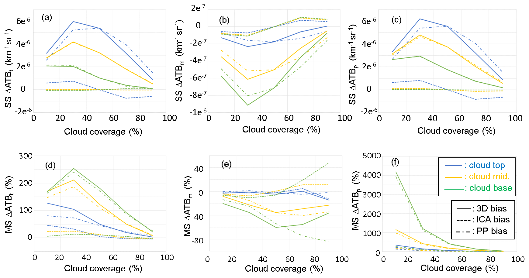
Figure 15ICA (dashed), PP (dotted dashed), and 3D (full line) biases under the single-scattering (SS) regime on (a) total ATB, (b) molecular ATB, and (c) particulate ATB as a function of cloud coverage (%) inside the lidar receiver FOV computed at cloud top (9.8 km, blue curves), in the middle of the cloud (9.5 km; yellow curves), and at cloud base (9.2 km; green curves). Panels (d), (e), and (f) are the same as (a), (b), and (c) but for relative bias and the MS regime. Cloud optical depth is 3.
Figure 15d and f show that MS total and particulate biases decrease when cloud coverage increases and reach almost zero for 90 % cloud coverage. These relative biases always show the largest values at cloud base, then in the middle of cloud, and then at cloud top, whereas it is not observed for SS bias (Fig. 15a and c). This is due to the division by reference ATB3D values that exponentially increase with cloud altitude. We also find that PP biases are positive, with a maximum bias of 250 % observed for the total relative ATB at cloud base and for cloud coverage of 30 %. These last two observations are consistent with simulation results under the SS regime: PP biases of total ATB and of particulate ATB are generally positive (see Eq. B8) and strictly positive (see Eq. B7), respectively. The maximum bias of ATB also occurs for cloud coverage of 30 %. Otherwise, regardless of cloud coverage, Fig. 15d and f show that MS total and particulate ICA biases are still rather small (<50 % and <200 %, respectively) compared to PP biases (<250 % and <4000 %, respectively). For total and particulate ATB, PP biases are the largest and are mainly responsible for the 3D biases, confirming the findings of the previous section for any cloud coverage in both the SS and MS regimes.
For molecular signals, Fig. 15e shows the negative PP bias that increases in absolute value with increasing cloud coverage, reaching −40 % and −80 % for 90 % cloud coverage in the middle of the cloud and at cloud base, respectively. The negative value of MS molecular PP bias is consistent with the SS molecular PP bias definition (see Eq. B6). Otherwise, MS ICA bias is negative for cloud coverage smaller than 50 % and rather positive for cloud coverage larger than 50 %. This latter observation is consistent with simulation results performed under SS regimes (see Fig. 15b): molecular ICA bias is negative, null, and positive for cloud coverage smaller than, equal to, and larger than 50 %, respectively. Figure 15e shows that MS ICA bias reaches only 15 % and 50 % in the middle of the cloud and at cloud base, respectively. At cloud top, all the molecular biases remain small (between 5 % and −15 %). Because of competition under the MS regime between the rather negative PP bias and the positive and negative ICA bias of the same order of magnitude, no specific trend in the 3D molecular biases according to the cloud coverage can be highlighted, and conclusions are less obvious than for total and particulate ATB.
Finally, our simulation results also show that 3D bias decreases in magnitude when COD decreases due to the PP bias that decreases. For example, if COD is 0.1, 3D total, molecular, and particulate biases are less than 6 %, 15 %, and 100 %, respectively, mainly driven by ICA bias.
3.3.2 Impact of the size of the field of view on total, molecular, and particulate ATB
We briefly investigate the impact of the size of the field of view (FOV) by carrying out simulations with an FOV 10 times greater than in the simulations performed in the previous sections. Simulations have been carried out for cloud coverage of 50 %, implying COD of 1.5 for the PP cloud model. Figure 16 shows vertical profiles of ATB biases and relative ATB biases computed with this large FOV (i.e., 650 µrad) and those computed with the ATLID FOV (i.e., 65 µrad).
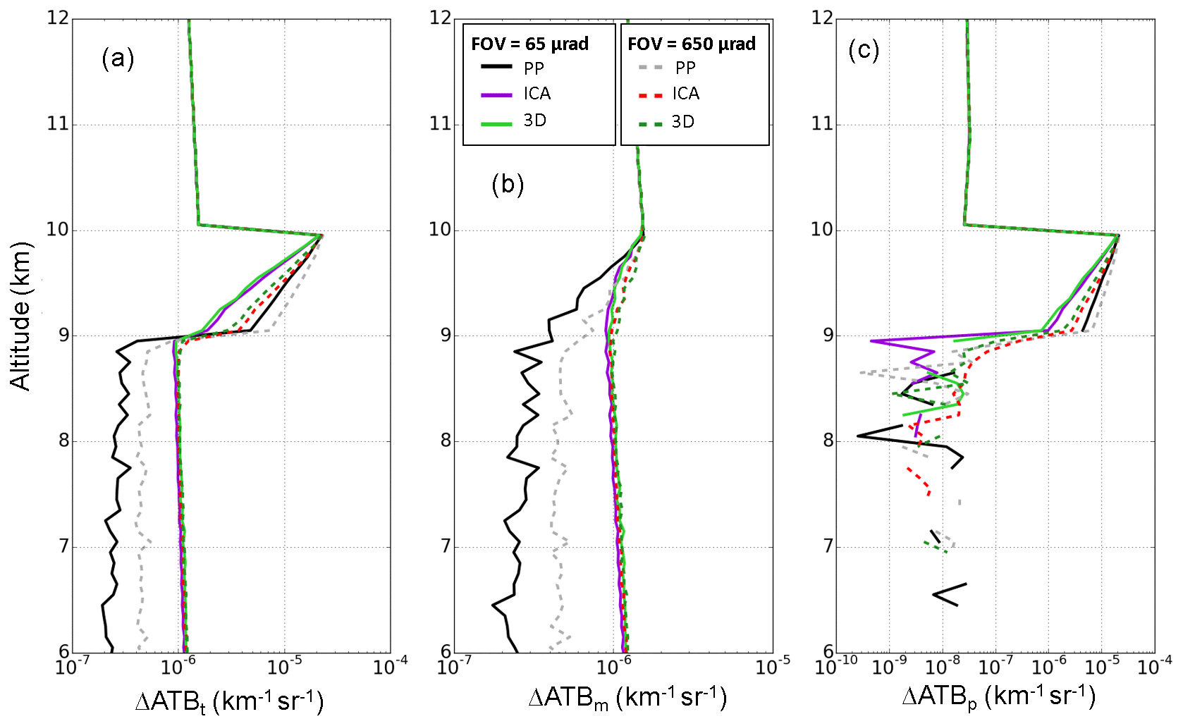
Figure 16Same as Fig. 13 but with 50 % cloud coverage. Simulations with ATLID FOV (65 µrad) are represented by full lines and simulations with a 650 µrad FOV are represented by dotted lines.
When comparing ATB computed with the three cloud models (i.e., PP, ICA, and 3D cloud model) for the large FOV, the same conclusions as for the ATLID FOV can be made: when reaching the cloud base, total and particulate ATBs show lower values for ICA and 3D models than for the PP model, and the opposite is true for the molecular ATB. Biases also show the same trend as for ATLID FOV, with a maximum bias for the PP model and lower values for ICA models.
When comparing simulations carried out with a large FOV to those performed with a small FOV, we observed that with a larger FOV, ATB values are larger when going into the cloud for the three cloud models. The reason is mainly the multiple scattering, which is obviously more pronounced as the FOV increases. Figure 16 shows that the biases and the relative biases for the large FOV present the same trend as for a small FOV. For total and particulate ATB, we can note that ICA biases are larger whatever the vertical position in the cloud, whereas PP biases are smaller in the upper part of the cloud due to multiple scattering, which becomes more significant as the FOV increases; this latter behavior is coherent with Eq. (B7). The relative biases for the large FOV show slightly smaller values for the three signal components (total, molecular, and particulate). The maximum values for the 3D bias are 150 %, −60 %, and 200 % for the total, molecular, and particulate ATBs, respectively.
Figure 17Same as Fig. 14 but with 50 % cloud coverage. Simulations with ATLID FOV (65 µrad) are represented by straight lines and simulations with a 650 µrad FOV are represented by dotted lines.
This paper presents the Monte Carlo code McRALI-FR that provides simulations of range-resolved z and frequency-resolved f Stokes parameters recorded by different kinds of monostatic polarized high-spectral-resolution lidars and Doppler radars from a 3D cloudy atmosphere and/or precipitation fields. McRALI-FR is an extension of 3DMcPOLID, a Monte Carlo code simulating a polarized active sensor (Alkasem et al., 2017). The core of McRALI-FR is based on the 3D polarized Monte Carlo atmospheric radiative transfer model 3DMCPOL (Cornet et al., 2010; Fauchez et al., 2014), which uses the local estimate method to reduce the noise level. Gas absorption in micro-wavelength is taken into account according to the work of Liebe (1985). McRALI-FR considers the Doppler effect related to the motion of hydrometeors and aerosols. The random motion, i.e., the turbulent flow, is assumed to be homogeneous and isotropic. It is modeled as a multivariate normal distribution. Generally, the regular motion of particles, i.e., the wind and/or precipitating hydrometeors, is assigned as a 3D vector field. The spectral distribution of the molecular scattering is modeled following the conventional method based on the Doppler shift from independent molecules moving with a Maxwell distribution of velocities. Each of the Stokes parameters is computed by McRALI-FR as a two-dimensional matrix (range- and frequency-resolved) and stored in an output file. Separate software uses the saved files to account for spectral and polarization characteristics of receivers and computes profiles of corresponding HSR lidar or Doppler radar signals.
A study has been carried out on the effects of NUBF on the HSR ATLID lidar and Doppler CPR radar signals of the EarthCARE mission with the help of the academic 3D box cloud, characterized by a single isolated jump in cloud optical depth. It is the simplest 3D cloud model that can be used to show and interpret the 3D radiative effects of clouds and for which the displayed results can only be obtained if the simulator is entirely in 3D. Moreover, for simplification, the wind speed is assumed to be only vertical and constant. Particle sedimentation velocity is null.
Regarding Doppler CPR radar signals, it appears that multiple scattering does not affect the velocity estimation when the cloud characteristics are locally homogeneous across the radar beam. But if vertical wind velocity sharply varies with altitude, the measured Doppler velocity profile can be largely affected by multiple-scattering processes, as already mentioned by Battaglia and Tanelli (2011). At the same time, it is confirmed that horizontally nonuniform beam filling induces a severe bias in velocity estimates. Indeed, the Doppler spectra shape is geometrically affected by the NUBF: the shape is all the more asymmetrical as the radar system vertically points away from the edge of the box cloud, inducing a bias in the estimation of the Doppler velocity. Within our very specific conditions of simulation with the box cloud and with McRALI-Fr code, we found a proportional coefficient value around 0.15 m s−1 (dBZ km close to that obtained by Sy et al. (2014) and Kollias et al. (2014).
Regarding HSR ATLID lidar signals, we confirm that multiple-scattering processes are not negligible, whatever the box-cloud cloud optical depth between 0.1 and 3, as previously studied by Reverdy et al. (2015) and pointed out by Donovan (2016). We also investigated the NUBF effect due to different cloud coverages inside the FOV on HSR ATLID lidar observables under the MS regime. For this purpose, we computed the vertical profiles of the 3D, PP, and ICA biases for total, molecular, and particulate ATB. The main conclusion is that 3D biases are mainly due to the PP biases, implying that NUBF effects are mainly due to unresolved variability of cloud inside the FOV and, to a lesser extent, to horizontal photon transport, which increases if FOV increases. Finally, these results give an indication of the reliability of lidar signals modeled using ICA.
All these simulations and results are still a test bench to show the ability of the McRALI-FR simulation tool to study the impact of multiple scattering and 3D cloud radiative effects on remote sensing observations and products. Real detailed cloud case studies and statistical analysis of representative fine-structure 3D cloud field effects on lidar and radar observables, while taking into account the polarization of light, will be the topic of future papers.
| Acronym | Definition |
| A-train | Afternoon constellation |
| ADM-Aeolus | Atmospheric Dynamics Mission |
| ALADIN | Atmospheric LAser Doppler Instrument |
| ATB | Attenuated backscatter |
| ATLID | ATmospheric LIDar |
| CALIPSO | Cloud–Aerosol Lidar and Infrared Pathfinder Satellite Observations |
| CNES | French National Centre for Space Studies |
| COD | Cloud optical depth |
| CPR | Cloud Profiling Radar |
| 3D | Three-dimensional |
| 3DMCPOL | 3D POLarized Monte Carlo atmospheric radiative transfer model |
| 3DMcPOLID | 3D Monte Carlo simulator of POLarized LIDar signals |
| DOMUS | Doppler multiple-scattering simulator |
| EECLAT | Expecting EarthCARE, Learning from A-train |
| EarthCARE | Earth Clouds, Aerosol and Radiation Explorer mission |
| ECSIM | EarthCARE simulator |
| ESA | European Space Agency |
| FOV | Field of view |
| ICA | Independent column approximation |
| INSU | French National Institute for Earth Sciences and Astronomy |
| HSR | High spectral resolution |
| MC | Monte Carlo |
| MS | Multiple scattering |
| McRALI | Monte Carlo modeling of RAdar and LIdar signals |
| McRALI-FR | McRALI Frequency-Resolved simulator |
| MUSCLE | MUltiple SCattering in Lidar Experiments |
| NUBF | Nonuniform beam filling |
| Probability density function | |
| PP | Plane-parallel and homogenous cloud |
| RTE | Radiative transfer equation |
| SS | Single scattering |
Total, molecular, and particulate ATB are hereafter noted ATBt, ATBm, and ATBp, respectively. According to Alkasem et al. (2017), PP bias can be understood from the following. Assuming null absorption and vertically constant atmospheric properties, then ATB(r)t at position r can be expressed as
where σm and σp are the molecular and particulate scattering coefficients, respectively, Pm and Pp are the molecular and particulate phase functions at 180∘, respectively, and γ is a factor that takes into account the multiple-scattering effects (Platt, 1973). In the same way, ATB(r)m and ATB(r)p, by voluntarily omitting r, assuming that σm and σp are vertically constant, and introducing the thickness Δr to lighten the writing, can be expressed as
Let α represent the cloud coverage inside the lidar receiver FOV; then the molecular (i.e., ATBm;IPA), particulate (i.e., ATBp;IPA), and total ATB (i.e., ATBt;IPA) computed with the IPA cloud model can be written as
and the molecular (i.e., ATBm;PP), particulate (i.e., ATBp;PP), and total (i.e., ATBt;PP) ATB computed with the PP cloud model can be written as
The PP molecular bias ΔATBm;PP, estimated as
is always negative. The PP particulate bias ΔATBp;PP, estimated as
is always positive. Note that the smaller γ is, the smaller ΔATBp;PP is. In other words, the larger the multiple-scattering effects, the smaller the PP particulate bias. The PP total bias ΔATBt;PP, estimated as
is positive but becomes negative with increasing cloud optical depth, as explained in Alkasem et al. (2017).
Fortran McRALI-FR codes can be obtained by contacting the corresponding author of this article.
FS, VS, and GM were responsible for the conceptual idea, supervision, and methodology. AA and GM conducted the numerical simulation and formal analysis. FS and GM acquired funding. All the authors contributed to developing the McRALI code and to writing and revising the paper.
The authors declare that they have no conflict of interest.
This work is part of the French scientific community EECLAT project (Expecting EarthCARE, Learning from A-train) (Luebke et al., 2018). The EECLAT community and research activities are supported by the National Center for Space Studies (CNES) and the National Institute for Earth Sciences and Astronomy (INSU). This work has also been supported in part by the Programme National de Télédétection Spatiale (PNTS, https://programmes.insu.cnrs.fr/pnts/, last access: 29 December 2020) under grant no. PNTS-2019-8.
This research has been supported by the National Institute for Earth Sciences and Astronomy (INSU grant) and the Programme National de Télédétection Spatiale (PNTS, https://programmes.insu.cnrs.fr/pnts/, last access: 29 December 2020) (grant no. PNTS-2019-8).
This paper was edited by Ad Stoffelen and reviewed by two anonymous referees.
Alkasem, A., Szczap, F., Cornet, C., Shcherbakov, V., Gour, Y., Jourdan, O., Labonnote, L. C., and Mioche, G.: Effects of cirrus heterogeneity on lidar CALIOP/CALIPSO data, J. Quant. Spectrosc. Ra., 202, 38–49, https://doi.org/10.1016/j.jqsrt.2017.07.005, 2017.
Amayenc, P., Marzoug, M., and Testud, J.: Analysis of cross-beam resolution effects in rainfall rate profile retrieval from a spaceborne radar, IEEE T. Geosci. Remote, 31, 417–425, https://doi.org/10.1109/36.214918, 1993.
Ansmann, A., Wandinger, U., Le Rille, O., Lajas, D., and Straume, A. G.: Particle backscatter and extinction profiling with the spaceborne high-spectral-resolution Doppler lidar ALADIN: methodology and simulations, Appl. Optics, 46, 6606, https://doi.org/10.1364/AO.46.006606, 2007.
Battaglia, A. and Tanelli, S.: DOMUS: Doppler Multiple-Scattering Simulator, IEEE T. Geosci. Remote, 49, 442–450, https://doi.org/10.1109/TGRS.2010.2052818, 2011.
Battaglia, A., Ajewole, M. O., and Simmer, C.: Evaluation of Radar Multiple-Scattering Effects from a GPM Perspective. Part I: Model Description and Validation, J. Appl. Meteorol. Clim., 45, 1634–1647, https://doi.org/10.1175/JAM2424.1, 2006.
Battaglia, A., Tanelli, S., Kobayashi, S., Zrnic, D., Hogan, R. J., and Simmer, C.: Multiple-scattering in radar systems: A review, J. Quant. Spectrosc. Ra., 111, 917–947, https://doi.org/10.1016/j.jqsrt.2009.11.024, 2010.
Battaglia, A., Tanelli, S., Mroz, K., and Tridon, F.: Multiple scattering in observations of the GPM dual-frequency precipitation radar: Evidence and impact on retrievals: MULTIPLE SCATTERING IN DPR OBSERVATIONS, J. Geophys. Res.-Atmos., 120, 4090–4101, https://doi.org/10.1002/2014JD022866, 2015.
Battaglia, A., Dhillon, R., and Illingworth, A.: Doppler W-band polarization diversity space-borne radar simulator for wind studies, Atmos. Meas. Tech., 11, 5965–5979, https://doi.org/10.5194/amt-11-5965-2018, 2018.
Bissonnette, L. R., Bruscaglioni, P., Ismaelli, A., Zaccanti, G., Cohen, A., Benayahu, Y., Kleiman, M., Egert, S., Flesia, C., Schwendimann, P., Starkov, A. V., Noormohammadian, M., Oppel, U. G., Winker, D. M., Zege, E. P., Katsev, I. L., and Polonsky, I. N.: LIDAR multiple scattering from clouds, Appl. Phys. B-Laser O., 60, 355–362, https://doi.org/10.1007/BF01082271, 1995.
Boucher, O., Randall, D., Artaxo, P., Bretherton, C., Feingold, G., Forster, P., Kerminen, V.-M., Kondo, Y., Liao, H., Lohmann, U., Rasch, P., Satheesh, S. K., Sherwood, S., Stevens, B., and Zhang, X. Y.: Clouds and Aerosols, in: Climate Change 2013: The Physical Science Basis. Contribution of Working Group I to the Fifth Assessment Report of the Intergovernmental Panel on Climate Change, edited by: Stocker, T. F., Qin, D., Plattner, G.-K., Tignor, M., Allen, S. K., Doschung, J., Nauels, A., Xia, Y., Bex, V., and Midgley, P. M., Cambridge University Press, Cambridge, UK, 571–658, 2014.
Bruneau, D. and Pelon, J.: Simultaneous measurements of particle backscattering and extinction coefficients and wind velocity by lidar with a Mach-Zehnder interferometer: principle of operation and performance assessment, Appl. Opt., 42, 1101, https://doi.org/10.1364/AO.42.001101, 2003.
Buras, R. and Mayer, B.: Efficient unbiased variance reduction techniques for Monte Carlo simulations of radiative transfer in cloudy atmospheres: The solution, J. Quant. Spectrosc. Ra., 112, 434–447, https://doi.org/10.1016/j.jqsrt.2010.10.005, 2011.
Cahalan, R. F., Ridgway, W., Wiscombe, W. J., Gollmer, S., and Harshvardhan: Independent Pixel and Monte Carlo Estimates of Stratocumulus Albedo, J. Atmos. Sci., 51, 3776–3790, https://doi.org/10.1175/1520-0469(1994)051<3776:IPAMCE>2.0.CO;2, 1994.
Cahalan, R. F., Oreopoulos, L., Marshak, A., Evans, K. F., Davis, A. B., Pincus, R., Yetzer, K. H., Mayer, B., Davies, R., Ackerman, T. P., Barker, H. W., Clothiaux, E. E., Ellingson, R. G., Garay, M. J., Kassianov, E., Kinne, S., Macke, A., O'hirok, W., Partain, P. T., Prigarin, S. M., Rublev, A. N., Stephens, G. L., Szczap, F., Takara, E. E., Várnai, T., Wen, G., and Zhuravleva, T. B.: The I3RC: Bringing Together the Most Advanced Radiative Transfer Tools for Cloudy Atmospheres, B. Am. Meteorol. Soc., 86, 1275–1294, https://doi.org/10.1175/BAMS-86-9-1275, 2005.
Chaikovskaya, L. I.: Remote sensing of clouds using linearly and circularly polarized laser beams: techniques to compute signal polarization, in: Light Scattering Reviews 3, edited by: Kokhanovsky, A. A., Springer Berlin and Heidelberg, Germany, 191–228, 2008.
Cornet, C., C.-Labonnote, L., and Szczap, F.: Three-dimensional polarized Monte Carlo atmospheric radiative transfer model (3DMCPOL): 3D effects on polarized visible reflectances of a cirrus cloud, J. Quant. Spectrosc. Ra., 111, 174–186, https://doi.org/10.1016/j.jqsrt.2009.06.013, 2010.
Davis, A. B. and Polonsky, I. N.: Approximation Methods in Atmospheric 3D Radiative Transfer Part 1: Resolved Variability and Phenomenology, in: 3D Radiative Transfer in Cloudy Atmospheres, edited by: Marshak, A. and Davis, A., Springer, Berlin and Heidelberg, Germany, 283–340, 2005.
de Mul, F. F. M., Koelink, M. H., Kok, M. L., Harmsma, P. J., Greve, J., Graaff, R., and Aarnoudse, J. G.: Laser Doppler velocimetry and Monte Carlo simulations on models for blood perfusion in tissue, Appl. Optics, 34, 6595, https://doi.org/10.1364/AO.34.006595, 1995.
Donovan, D., Voors, R., van Zadelhoff, G.-J., and Acarreta, J.-R.: ECSIM Model and Algorithms Document, KNMI Tech. Rep.: ECSIM-KNMI-TEC-MAD01-R, available at: https://www.knmi.nl/kennis-en-datacentrum/publicatie/ecsim-model-and-algorithms-document (last access: 16 April 2019), 2008.
Donovan, D. P.: The Expected Impact of Multiple Scattering on ATLID Signals, Web of Conferences, 119, 01006, https://doi.org/10.1051/epjconf/201611901006, 2016.
Donovan, D. P., Klein Baltink, H., Henzing, J. S., de Roode, S. R., and Siebesma, A. P.: A depolarisation lidar-based method for the determination of liquid-cloud microphysical properties, Atmos. Meas. Tech., 8, 237–266, https://doi.org/10.5194/amt-8-237-2015, 2015
Doviak, R. J. and Zrnić, D. S.: Doppler radar and weather observations, Academic Press, Orlando, FL, USA, 1984.
Dubovik, O., Sinyuk, A., Lapyonok, T., Holben, B. N., Mishchenko, M., Yang, P., Eck, T. F., Volten, H., Muñoz, O., Veihelmann, B., van der Zande, W. J., Leon, J.-F., Sorokin, M., and Slutsker, I.: Application of spheroid models to account for aerosol particle nonsphericity in remote sensing of desert dust, J. Geophys. Res., 111, D11208, https://doi.org/10.1029/2005JD006619, 2006.
Dufresne, J.-L. and Bony, S.: An Assessment of the Primary Sources of Spread of Global Warming Estimates from Coupled Atmosphere–Ocean Models, J. Climate, 21, 5135–5144, https://doi.org/10.1175/2008JCLI2239.1, 2008.
Durden, S. L., Haddad, Z. S., Kitiyakara, A., and Li, F. K.: Effects of Nonuniform Beam Filling on Rainfall Retrieval for the TRMM Precipitation Radar, J. Atmos. Oceanic Tech., 15, 635–646, https://doi.org/10.1175/1520-0426(1998)015<0635:EONBFO>2.0.CO;2, 1998.
Emde, C., Buras, R., and Mayer, B.: ALIS: An efficient method to compute high spectral resolution polarized solar radiances using the Monte Carlo approach, J. Quant. Spectrosc. Ra., 112, 1622–1631, https://doi.org/10.1016/j.jqsrt.2011.03.018, 2011.
ESA: European Space Agency (ESA): ADM-Aeolus Mission Requirements Document, ESA EOP-SM/2047, available at: http://esamultimedia.esa.int/docs/EarthObservation/ADM-Aeolus_MRD.pdf (last ccess: 16 April 2019), 2016.
ESA report: ADM-Aeolus Mission Requirements Document, ESA EOP-SM/2047, available at: http://esamultimedia.esa.int/docs/EarthObservation/ADM-Aeolus_MRD.pdf (last access: 16 April 2019), 2016.
Evans, K. F. and Marshak, A.: Numerical methods, in: 3D Radiative transfer in cloudy atmosphere, edited by: Marshak, A. and Davis, A. B., Springer, 243–281, 2005
Fauchez, T., Cornet, C., Szczap, F., Dubuisson, P., and Rosambert, T.: Impact of cirrus clouds heterogeneities on top-of-atmosphere thermal infrared radiation, Atmos. Chem. Phys., 14, 5599–5615, https://doi.org/10.5194/acp-14-5599-2014, 2014.
Gayet, J.-F.: Cirrus cloud microphysical and optical properties at southern and northern midlatitudes during the INCA experiment, J. Geophys. Res., 109, D20206, https://doi.org/10.1029/2004JD004803, 2004.
Hansen, J. E. and Travis, L. D.: Light scattering in planetary atmospheres, Space Sci. Rev., 16, 527–610, https://doi.org/10.1007/BF00168069, 1974.
Hélière, A., Le Hors, L., and Toulemont, Y.: Development of ATLID, the earthcare UV backscatter lidar, in: Proc. SPIE 10563, International Conference on Space Optics – ICSO 2014, 105633R, https://doi.org/10.1117/12.2304087, 2017.
Hilsenrath, E. and Ward, A. B.: The Third A-Train Symposium: Summary and Perspectives on a Decade of Constellation-Based Earth Observations, available at: https://eospso.nasa.gov/sites/default/files/eopdfs/July%20August%202017%20color%20508.pdf (last access: 16 April 2019), 2017.
Hogan, R. J.: Fast Lidar and Radar Multiple-Scattering Models. Part I: Small-Angle Scattering Using the Photon Variance-Covariance Method, J. Atmos. Sci., 65, 3621–3635, https://doi.org/10.1175/2008JAS2642.1, 2008.
Hogan, R. J. and Battaglia, A.: Fast Lidar and Radar Multiple-Scattering Models. Part II: Wide-Angle Scattering Using the Time-Dependent Two-Stream Approximation, J. Atmos. Sci., 65, 3636–3651, https://doi.org/10.1175/2008JAS2643.1, 2008.
Hu, Y.-X., Winker, D., Yang, P., Baum, B., Poole, L., and Vann, L.: Identification of cloud phase from PICASSO-CENA lidar depolarization: a multiple scattering sensitivity study, J. Quant. Spectrosc. Ra., 70, 569–579, https://doi.org/10.1016/S0022-4073(01)00030-9, 2001.
Iguchi, T., Kozu, T., Meneghini, R., Awaka, J., and Okamoto, K.: Rain-Profiling Algorithm for the TRMM Precipitation Radar, J. Appl. Meteorol., 39, 2038–2052, https://doi.org/10.1175/1520-0450(2001)040<2038:RPAFTT>2.0.CO;2, 2000.
Iguchi, T., Kozu, T., Kwiatkowski, J., Meneghini, R., Awaka, J., and Okamoto, K.: Uncertainties in the Rain Profiling Algorithm for the TRMM Precipitation Radar, J. Meteorol. Soc. Jpn., 87, 1–30, https://doi.org/10.2151/jmsj.87A.1, 2009.
Illingworth, A. J., Barker, H. W., Beljaars, A., Ceccaldi, M., Chepfer, H., Clerbaux, N., Cole, J., Delanoë, J., Domenech, C., Donovan, D. P., Fukuda, S., Hirakata, M., Hogan, R. J., Huenerbein, A., Kollias, P., Kubota, T., Nakajima, T., Nakajima, T. Y., Nishizawa, T., Ohno, Y., Okamoto, H., Oki, R., Sato, K., Satoh, M., Shephard, M. W., Velázquez-Blázquez, A., Wandinger, U., Wehr, T., and van Zadelhoff, G.-J.: The EarthCARE Satellite: The Next Step Forward in Global Measurements of Clouds, Aerosols, Precipitation, and Radiation, B. Am. Meteorol. Soc., 96, 1311–1332, https://doi.org/10.1175/BAMS-D-12-00227.1, 2015.
Ishimoto, H. and Masuda, K.: A Monte Carlo approach for the calculation of polarized light: application to an incident narrow beam, J. Quant. Spectrosc. Ra., 72, 467–483, https://doi.org/10.1016/S0022-4073(01)00136-4, 2002
Kobayashi, S., Kumagai, H., and Iguchi, T.: Accuracy Evaluation of Doppler Velocity on a Spaceborne Weather Radar through a Random Signal Simulation, J. Atmos. Ocean. Tech., 20, 944–949, https://doi.org/10.1175/1520-0426(2003)020<0944:AEODVO>2.0.CO;2, 2003.
Kollias, P., Tanelli, S., Battaglia, A., and Tatarevic, A.: Evaluation of EarthCARE Cloud Profiling Radar Doppler Velocity Measurements in Particle Sedimentation Regimes, J. Atmos. Ocean. Tech., 31, 366–386, https://doi.org/10.1175/JTECH-D-11-00202.1, 2014.
Kollias, P., Battaglia, A., Tatarevic, A., Lamer, K., Tridon, F., and Pfitzenmaier, L.: The EarthCARE cloud profiling radar (CPR) doppler measurements in deep convection: challenges, post-processing, and science applications, in: Proc. SPIE 10776, Remote Sensing of the Atmosphere, Clouds, and Precipitation VII, 107760R, https://doi.org/10.1117/12.2324321, 2018.
Lenoble, J.: Atmospheric radiative transfer, Deepak, Hampton, Va, 1993.
Liebe, H. J.: An updated model for millimeter wave propagation in moist air, Radio Sci., 20, 1069–1089, https://doi.org/10.1029/RS020i005p01069, 1985.
Liou, K.-N.: An introduction to atmospheric radiation, 2nd edn., Academic Press, Amsterdam, 2002.
Luebke, A. E., Delanoë, J., Noel, V., Chepfer, H., and Stevens, B.: A Workshop on Remote Sensing of the Atmosphere in Anticipation of the EarthCARE Satellite Mission, B. Am. Meteorol. Soc., 99, 195–198, https://doi.org/10.1175/BAMS-D-18-0143.1, 2018.
Marchuk, G. I., Mikhailov, G. A., Nazareliev, M. A., Darbinjan, R. A., and Elepov, B. S.: The Monte Carlo method in atmospheric optics, Springer Berlin Heidelberg, 1980.
Marshak, A. and Davis, A.: 3D Radiative Transfer in Cloudy Atmospheres, Springer, Berlin and Heidelberg, Germany, 2005.
Mayer, B.: Radiative transfer in the cloudy atmosphere, Eur. Physical J. Conf., 1, 75–99, https://doi.org/10.1140/epjconf/e2009-00912-1, 2009.
Miller, S. D. and Stephens, G. L.: Multiple scattering effects in the lidar pulse stretching problem, J. Geophys. Res.-Atmos., 104, 22205–22219, https://doi.org/10.1029/1999JD900481, 1999.
Noel, V., Chepfer, H., Ledanois, G., Delaval, A., and Flamant, P. H.: Classification of particle effective shape ratios in cirrus clouds based on the lidar depolarization ratio, Appl. Optics, 41, 4245, https://doi.org/10.1364/AO.41.004245, 2002.
Partain, P. T., Heidinger, A. K., and Stephens, G. L.: High spectral resolution atmospheric radiative transfer: Application of the equivalence theorem, J. Geophys. Res.-Atmos., 105, 2163–2177, https://doi.org/10.1029/1999JD900328, 2000.
Pereira do Carmo, J., de Villele, G., Helière, A., Wallace, K., Lefebvre, A., and Chassat, F.: ATLID, ESA atmospheric backscatter LIDAR for the ESA EarthCARE mission, CEAS Space J., 11, 423–435, https://doi.org/10.1007/s12567-019-00284-6, 2019.
Platt, C. M. R.: Lidar and Radioinetric Observations of Cirrus Clouds, J. Atmos. Sci., 30, 1191–1204, https://doi.org/10.1175/1520-0469(1973)030<1191:LAROOC>2.0.CO;2, 1973.
Reitebuch, O., Huber, D., and Nikolaus, I.: ADM-Aeolus Algorithm Theoretical Basis Document (ATBD) Level1B Products, AE-RPDLR- L1B-001, 4.4, 117 pp., available at: https://earth.esa.int/pi/esa?type=file&table=aotarget&cmd=image&alias=Aeolus_L1B_Algorithm_TBD (last access: 23 September 2020), 2018.
Reverdy, M., Chepfer, H., Donovan, D., Noel, V., Cesana, G., Hoareau, C., Chiriaco, M., and Bastin, S.: An EarthCARE/ATLID simulator to evaluate cloud description in climate models: AN EARTHCARE/ATLID SIMULATOR, J. Geophys. Res.-Atmos., 120, 11090-11113, https://doi.org/10.1002/2015JD023919, 2015.
Sato, K., Okamoto, H., and Ishimoto, H.: Modeling the depolarization of space-borne lidar signals, Opt. Express, 27, A117, https://doi.org/10.1364/OE.27.00A117, 2019.
Shcherbakov, V., Gayet, J.-F., Jourdan, O., Ström, J., and Minikin, A.: Light scattering by single ice crystals of cirrus clouds, Geophys. Res. Lett., 33, L15809, https://doi.org/10.1029/2006GL026055, 2006.
Shipley, S. T., Tracy, D. H., Eloranta, E. W., Trauger, J. T., Sroga, J. T., Roesler, F. L., and Weinman, J. A.: High spectral resolution lidar to measure optical scattering properties of atmospheric aerosols 1: Theory and instrumentation, Appl. Optics, 22, 3716, https://doi.org/10.1364/AO.22.003716, 1983.
Stephens, G., Winker, D., Pelon, J., Trepte, C., Vane, D., Yuhas, C., L'Ecuyer, T., and Lebsock, M.: CloudSat and CALIPSO within the A-Train: Ten Years of Actively Observing the Earth System, B. Am. Meteorol. Soc., 99, 569–581, https://doi.org/10.1175/BAMS-D-16-0324.1, 2018.
Stephens, G. L., Vane, D. G., Tanelli, S., Im, E., Durden, S., Rokey, M., Reinke, D., Partain, P., Mace, G. G., Austin, R., L'Ecuyer, T., Haynes, J., Lebsock, M., Suzuki, K., Waliser, D., Wu, D., Kay, J., Gettelman, A., Wang, Z., and Marchand, R.: CloudSat mission: Performance and early science after the first year of operation, J. Geophys. Res., 113, D00A18, https://doi.org/10.1029/2008JD009982, 2008.
Stoffelen, A., Pailleux, J., Källén, E., Vaughan, J. M., Isaksen, L., Flamant, P., Wergen, W., Andersson, E., Schyberg, H., Culoma, A., Meynart, R., Endemann, M., and Ingmann, P.: THE ATMOSPHERIC DYNAMICS MISSION FOR GLOBAL WIND FIELD MEASUREMENT, B. Am. Meteorol. Soc., 86, 73–88, https://doi.org/10.1175/BAMS-86-1-73, 2005.
Sy, O. O., Tanelli, S., Takahashi, N., Ohno, Y., Horie, H., and Kollias, P.: Simulation of EarthCARE Spaceborne Doppler Radar Products Using Ground-Based and Airborne Data: Effects of Aliasing and Nonuniform Beam-Filling, IEEE T. Geosci. Remote, 52, 1463–1479, https://doi.org/10.1109/TGRS.2013.2251639, 2014.
Tanelli, S., Im, E., Durden, S. L., Facheris, L., and Giuli, D.: The Effects of Nonuniform Beam Filling on Vertical Rainfall Velocity Measurements with a Spaceborne Doppler Radar, J. Atmos. Ocean. Tech., 19, 1019–1034, https://doi.org/10.1175/1520-0426(2002)019<1019:TEONBF>2.0.CO;2, 2002.
Testud, J., Amayenc, P., Dou, X., and Tani, T.: Tests of Rain Profiling Algorithms for a Spaceborne Radar Using Raincell Models and Real Data Precipitation Fields, J. Atmos. Ocean. Tech., 13, 426–453, https://doi.org/10.1175/1520-0426(1996)013<0426:TORPAF>2.0.CO;2, 1996.
Tipler, P. A. and Mosca, G.: Physics for scientists and engineers: standard, 6th ed., W.H. Freeman, New York, NY, USA, 2008.
Tong, Y. L.: The Multivariate Normal Distribution, Springer, New York, NY, USA, 1990.
Vallée, O. and Soares, M.: Airy functions and applications to physics, World Scientific, New Jersey, USA, 2004.
Weitkamp, C.: Lidar Range-Resolved Optical Remote Sensing of the Atmosphere, Springer-Verlag New York, 2005.
Wilczek, M., Daitche, A., and Friedrich, R.: On the velocity distribution in homogeneous isotropic turbulence: correlations and deviations from Gaussianity, J. Fluid Mech., 676, 191–217, https://doi.org/10.1017/jfm.2011.39, 2011.
Winker, D. M., Pelon, J., Coakley, J. A., Ackerman, S. A., Charlson, R. J., Colarco, P. R., Flamant, P., Fu, Q., Hoff, R. M., Kittaka, C., Kubar, T. L., Le Treut, H., Mccormick, M. P., Mégie, G., Poole, L., Powell, K., Trepte, C., Vaughan, M. A., and Wielicki, B. A.: The CALIPSO Mission: A Global 3D View of Aerosols and Clouds, B. Am. Meteorol. Soc., 91, 1211–1230, https://doi.org/10.1175/2010BAMS3009.1, 2010.
Yang, P. and Liou, K. N.: Geometric-optics-integral-equation method for light scattering by nonspherical ice crystals, Appl. Optics, 35, 6568, https://doi.org/10.1364/AO.35.006568, 1996.
Zrnic, D.: Spectral Moment Estimates from Correlated Pulse Pairs, IEEE T. Aero. Elec. Sys., 13, 344–354, https://doi.org/10.1109/TAES.1977.308467, 1977.
- Abstract
- Introduction
- Modeling of HSR lidar and Doppler radar signals with McRALI
- Assessment of errors induced by NUBF on lidar and radar data
- Conclusions
- Appendix A: List of acronyms used in this work and their definition
- Appendix B: Estimation of the PP bias of molecular, particulate, and total ATB as a function of cloud coverage and multiple-scattering intensity for the box-cloud model
- Code availability
- Author contributions
- Competing interests
- Acknowledgements
- Financial support
- Review statement
- References