the Creative Commons Attribution 4.0 License.
the Creative Commons Attribution 4.0 License.
 | 18 May 2021
Insights into wind turbine reflectivity and radar cross-section (RCS) and their variability using X-band weather radar observations
Martin Lainer
Jordi Figueras i Ventura
Zaira Schauwecker
Marco Gabella
Montserrat F.-Bolaños
Reto Pauli
Jacopo Grazioli
The increasing need of renewable energy fosters the expansion of wind turbine sites for power production throughout Europe with manifold effects, both on the positive and negative side. The latter concerns, among others, radar observations in the proximity of wind turbine (WT) sites. With the aim of better understanding the effects of large, moving scatterers like wind turbines on radar returns, MeteoSwiss performed two dedicated measurement campaigns with a mobile X-band Doppler polarimetric weather radar (METEOR 50DX) in the northeastern part of Switzerland in March 2019 and March 2020. Based on the usage of an X-band radar system, the performed campaigns are up to now unique. The main goal was to quantify the effects of wind turbines on the observed radar moments, to retrieve the radar cross-section (RCS) of the turbines themselves and to investigate the conditions leading to the occurrence of the largest RCS. Dedicated scan strategies, consisting of PPI (plan position indicator), RHI (range–height indicator) and fixed-pointing modes, were defined and used for observing a wind park consisting of three large wind turbines. During both campaigns, measurements were taken in operation. The highest measured maxima of horizontal reflectivity (ZH) and RCS reached 78.5 dBZ and 44.1 dBsm, respectively. A wind turbine orientation (yawing) stratified statistical analysis shows no clear correlation with the received maximum returns. However, the median values and 99th percentiles of ZH show different enhancements for specific relative orientations. Some of them remain still for Doppler-filtered data, supporting the importance of the moving parts of the wind turbine for the radar returns. Further, we show, based on investigating correlations and an OLS (ordinary least square) model analysis, that the fast-changing rotor blade angle (pitch) is a key parameter, which strongly contributes to the variability in the observed returns.
- Article
(11360 KB) - Full-text XML
- BibTeX
- EndNote


The rapid development and expansion of wind farms in the latest years are a significant source of concern for the weather (e.g., Norin, 2017) and aviation radar community (de la Vega et al., 2016; Cuadra et al., 2019). Wind turbines are very large, reflective and moving objects, which makes them a source of clutter that becomes difficult to filter or separate from return signals of interest. Over the last years, the demand for the quantification, modeling and mitigation of the effects of wind turbines on radar systems has been rising as the number of installed, planned or foreseen wind turbines is highly increasing. As analyzed by Komusanac et al. (2020) in 2019, about 15.4 GW of new wind power capacity was installed in the European Union (EU). This is 27 % higher than in 2018. The total capacity of wind energy in the EU at the end of 2019 was 205 GW. The effective real production amounts to about 417 TWh, which is 15 % of the total consumed electricity. With the fact that green energy is becoming trendy, a realistic outlook until 2030 is to have around 323 GW of wind turbine power installed (Nghiem et al., 2017). By assuming a perfectly rational market here, it is expected that more wind turbines will pop up.
Several studies exist in the literature about the evaluation and quantification of the impact of wind turbines on radar systems. These studies discussed the issue of clutter contamination of weather radar data (Lepetit et al., 2019; Hood et al., 2010; Angulo et al., 2015) as well as the identification of adverse effects of wind turbines on the performance of air surveillance and marine radars (Angulo et al., 2014; Cuadra et al., 2019). In general, wind turbine clutter reflectivity depends on various parameters such as wind turbine dimensions, incidence angle of radiation, rotor speed, nacelle orientation and radiation frequency (Gallardo-Hernando et al., 2011; Norin, 2015).
A key parameter for the evaluation of how efficiently electromagnetic waves interfere with a physical object is the radar cross-section (RCS). RCS is an optimal variable to estimate the effect of a “point target” on the performance of a radar system. With the term “point” we mean a target which is much smaller than the radar sampling volume and with a size such that the incident field could be assumed to be planar over the whole extent of the target. However, the RCS concept is often generalized and extended to larger objects, starting with small airplanes but then reaching even large airplanes and wind turbines. As a matter of fact, existing numerical models for estimating the backscattering efficiency of wind turbines rely on this quantity. It is the projected area needed to isotropically re-irradiate the same power as the target scatters in the direction of the receiver and is usually expressed in decibel units related to 1 m2 (dBsm) (Knott et al., 2004; Skolnik, 1990). The detailed background on how the RCS is computed within our system is given in Sect. 3. A lot of studies have been published evaluating the RCS of individual wind turbines and wind farms and the effects on radar and communication systems. For instance, Lute and Wieserman (2011), Kong et al. (2011), and Kent et al. (2008) have used measurements to characterize wind turbine scattering properties and the impact on radar performance. Others used numerical tools to investigate RCS and Doppler signatures of model-based wind turbines (de la Vega et al., 2016; Muñoz-Ferreras et al., 2016; He et al., 2015). The electromagnetic interactions between wind turbines and radar signals are complex and the general understanding still limited.
In this work effort was put into the analysis of the data of two dedicated field campaigns which took place in March 2019 and March 2020, aiming at gathering weather radar measurements in the X-band frequency of three large wind turbines. The primary focus of this paper is to present a statistical analysis of radar reflectivity (ZH) and retrieved RCS values and to find the relation between those variables and the operational data of the wind turbines (orientation, blade pitch angle, revolution speed).
In Sect. 2 we describe the field campaigns and X-band weather radar system used in this study (METEOR 50DX) as well as some key parameters of the wind turbine targets. More details on the observation site and visibility towards the wind park are given in Sect. 2.1. The special scanning strategies are the topic of Sect. 2.2, while the data sets are briefly treated in Sect. 2.3. In Sect. 3 we first present global statistics regarding unfiltered horizontal reflectivity ZH for all three wind turbines during the field campaign in 2019. For simplicity, we call ZH just horizontal reflectivity hereinafter, for which no Doppler or any other quality filter is applied. With data from the March 2020 campaign, the impact of the relative (with respect to the radar location) nacelle orientation (yaw angle), blade orientation (pitch angle), rotor revolutions and wind speed on the received radar returns is investigated by different correlation analyses (Sect. 3.2). The impact of a Doppler notch clutter filter on parts of the post-processed data is discussed. To even better explain the variance of the maximum ZH, an OLS (ordinary least square) model fit is performed (Sect. 3.3). Finally, in Sect. 4 a summary and conclusion are provided.
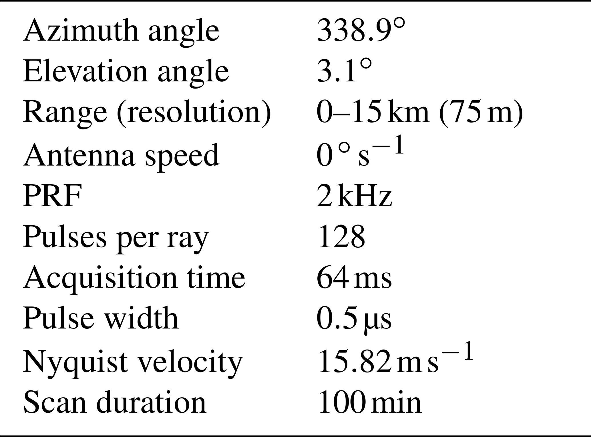
The main goal of the measurement campaigns in 2019 and 2020 was to study the interaction between electromagnetic waves at 9.84 GHz sent by the weather radar and the structure of wind turbines. For this type of investigation, a small wind park consisting of three large wind turbines, with the characteristics specified in Table 1, was selected near the city of Schaffhausen. Many logistical requirements for the installation of the weather radar had to be met (e.g., sufficient power supply, radiation safety, permits from the Swiss Federal Office of Communication) in addition to good visibility towards the wind park. More details on the observation site are provided in Sect. 2.1.
Table 1Specifications of the wind turbines in the observed wind park during the measurement campaigns in 2019 and 2020.

The field campaign in 2019 took place between 6 and 28 March with totally 23 d of continuous observations, while the second one took place between 4 and 25 March 2020 with a total of 22 d of measurements. During the latter campaign, the radar data were collected with a fixed-pointing antenna towards the nacelle of the closest wind turbine with respect to the radar site. The radar scanning protocol lasted 120 min, whereof 100 min were used for the fixed-pointing measurements and about 12 min for a PPI (plan position indicator) volume acquisition as an overview scan for the whole wind park area.
The measurements presented in this paper have been collected with a dual-polarization, simultaneous transmission and reception (STAR), mobile Doppler weather radar, which operates at a frequency of 9.48 GHz (X-band). This radar system is sensitive mostly to hydrometeors in the precipitation size range. Due to the relatively small antenna size and overall weight, it is a transportable system integrated into a trailer and particularly suitable for field campaigns and agile relocations. Several configurations of the transmission protocols and data acquisition can be defined (e.g., pulse repetition frequency – PRF, pulse widths, scan velocity, data acquisition rate). For the campaigns we are consistent and stick to one pulse width of 0.5 µs to have a good target range resolution of 75 m, where most of the radiation energy is scattered by the WT object. The 0.5 µs pulse shape is, compared to the one for 0.33 µs, more uniform and thus preferred in our system. The antenna movement for the measurements in 2019 is slow, ensuring data collection every 0.1∘ in azimuth, while the PRF is set high enough (2 kHz) to ensure a large number of pulses for each radial and a reasonably good unambiguous velocity range. A detailed technical overview about the characteristics of the radar system can be found in Neely et al. (2018). Some key specifications are listed in Table 2.
Table 2Specifications of the mobile METEOR 50DX dual-polarization weather radar used for the measurement campaigns in 2019 and 2020. The abbreviations H and V stand for horizontal and vertical polarization, respectively.

The radar system provides a set of single-polarization, dual-polarization and Doppler measurements: horizontal (vertical) reflectivity ZH (ZV), differential reflectivity ZDR, co-polar correlation coefficient ρHV, total differential phase shift ΦDP, specific differential phase shift KDP, Doppler velocity V and Doppler spectrum width W. If filters or thresholds are applied to the data, not only the filtered data can be kept but also always the raw data. Additionally it is possible to store full power spectrum (PSR) data.
After the wind turbine campaign in 2019 two main upgrades of our mobile radar system have been conducted. In June a complete new seamless radome was installed. The improvements compared to the former radome, which was joined by metal units, are shown and discussed in Figueras i Ventura et al. (2020b). Concerning power-related measurements, it is important to know that the attenuation of both radomes have similar values. Later in October, an important software upgrade was performed, allowing now the acquisition of data when the radar antenna is not moving (something that was not possible to do in 2019). This new ability is hereafter referred to as fixed-pointing or stare-mode measurements of the weather radar.
The core data processing for both campaigns was done by the MeteoSwiss in-house-developed open-source real-time weather radar data processing framework Pyrad (Figueras i Ventura et al., 2020a), which is based on the Py-ART radar toolkit (Helmus and Collis, 2016).
2.1 Observation site and radar visibility
The observation site where the radar system could be installed was in the vicinity of the city of Schaffhausen. This site had several advantages: line of sight with the wind turbines, a minimum distance from the wind park to limit the risk of a receiver saturation, site accessibility, permission to transmit and power connection. The three wind turbines of the small wind park located north of Schaffhausen are installed on a hill surrounded by forests. The corresponding terrain profile between the radar and the furthermost wind turbine (WT3) is shown in Fig. 1c. The locations of the turbines as seen from the radar site are at distances of 7.7, 8.1 and 8.6 km with directions of 337.8, 343.3 and 340.2∘ from the north. In order to hit the turbine ground locations, elevation angles of 2.24∘ (WT1) and 2.1∘ (WT2, WT3) are needed.
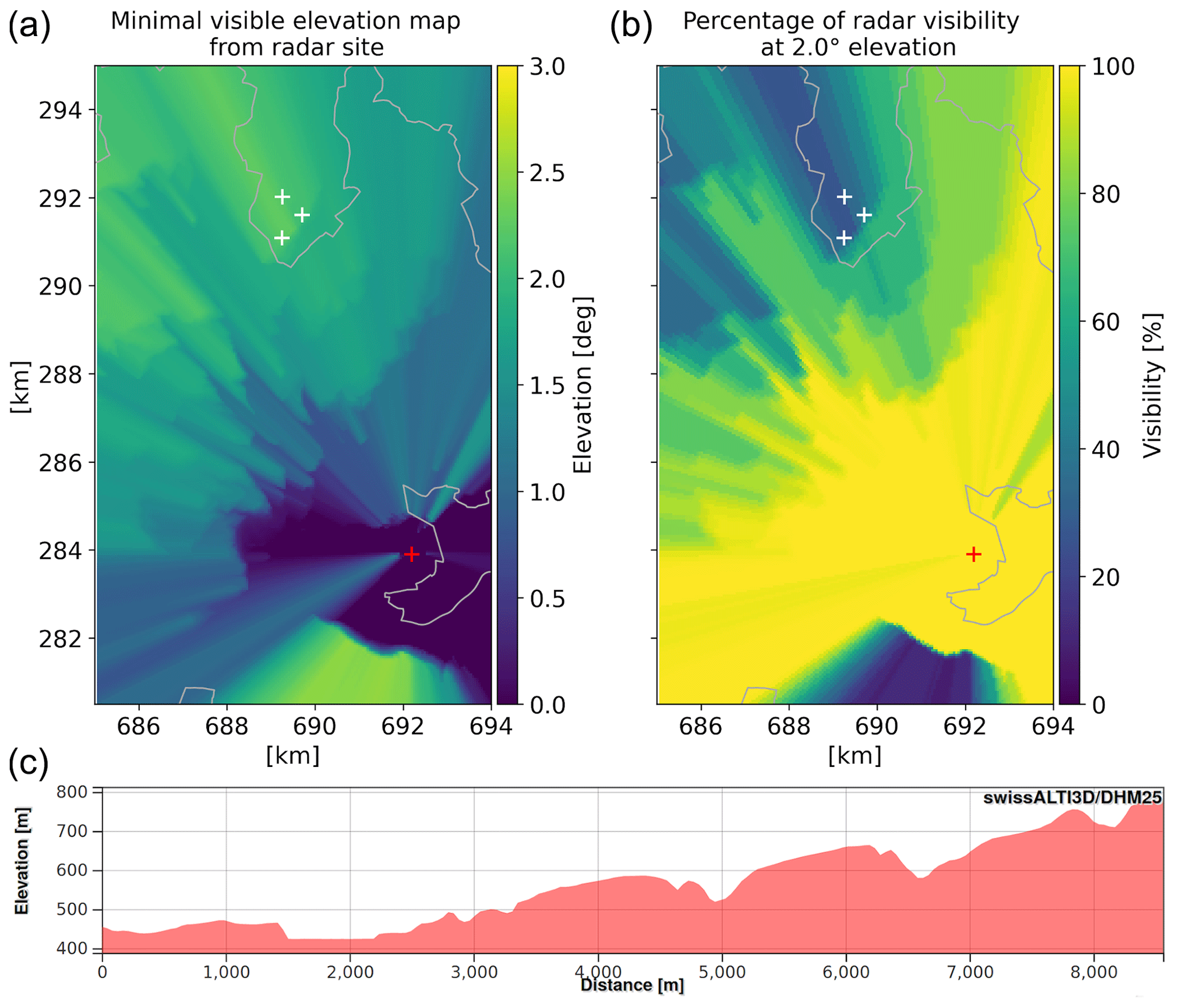
Figure 1Visibility contour maps from DEM-based GECSX (Ground Echo Clutter Simulator) simulations for the radar observation site close to Schaffhausen. Minimal-visibility map (elevation for maximum of 50 % beam blockage) is shown in plot (a). Plot (b) shows the derived percentages of visibility for the fixed antenna elevation of 2.0∘. White plus signs indicate the wind turbine locations and the red plus signs the weather radar location. Additionally the cross-section of the terrain profile between the radar observation site (left end of cross-section) and the wind turbine of the wind park with the largest distance to the radar (right end of cross-section) is presented in (c). The last plot was produced on the swisstopo website (https://www.geo.admin.ch/, last access: 21 March 2021).
Although trees were blocking part of the radiation towards the masts at a distance of 1 km, the rotor centers of all three wind turbines were always visible at the center of the radar antenna beam. With radar ground echo clutter simulations based on GECSX (Ground Echo Clutter Simulator) and a digital elevation model (DEM) with 50 m resolution, the radar visibility towards the wind turbines could be determined. The used approach follows the technique and developed software described in Gabella and Perona (1998) and Gabella et al. (2008). Figure 1a shows the minimal-visibility elevation map, which is the minimum radar antenna beam elevation angle to get maximum 50 % beam blockage, starting from the weather radar observation site. The locations of the wind turbines are indicated as three white plus signs in the maps, while the radar location is shown as a red plus sign. From the first map (Fig. 1a) we get the lowest elevation angles with visibility at the center of the radar beam: 2.25∘ (WT1), 2.10 ∘ (WT2) and 2.15∘ (WT3). With increasing elevation of the radar beam the visibility gets better (see Fig. 1b). At an elevation of 3∘, all three turbine locations are visible with the whole HPBW (half-power beam width) angle.
Given the distances to the wind turbines, ranging between 7.7 and 8.6 km with respect to the radar site, together with the characteristics of the radar antenna (HPBW of 1.25∘), a beam broadening between 175 and 195 m can be assumed at the ranges of the wind turbines. Compared to the spatial dimensions of the wind turbines, the beam shape is already larger when it is reaching the target. Due to the fact that the radar measurements are the result of a convolution between the beam shape and wind turbine structures, it is difficult to distinguish return signals from structures that are smaller than the beam shape during the radar scans.
2.2 Radar scanning strategy
The scanning strategy of the weather radar system in 2019 consisted of the continuous repetition of a protocol lasting 45 min, including three different scan types: PPI, RHI (range–height indicator) and solar scan. While the PPI and RHI scans were dedicated to the wind turbine measurements, the solar scan is used for the receiver quality control. One PPI sector scan sequence lasted 12 min; one RHI scan sequence took 18 min.
The sequence of PPI scans is a narrow-volume scan in the azimuth sector 331 to 349∘ consisting of 30 individual PPIs at increasing elevation angles. Regarding the RHI scans, a sequence of 81 individual RHIs were set up. The RHI scans are separated by 0.2∘ at the edges of the azimuthal scan area and 0.1∘ in the core region. In order to optimize the mechanical antenna movements of the scans, the RHIs are conducted from the smallest to the largest azimuth angle with alternating upward and downward antenna motions, which create a continuous sampling of the volume. With the use of RHI scans, a better characterization of the influence of the secondary lobes towards the ground is possible.
The detailed parameters of both scan types are listed in Table 3. The movement of the antenna is slow for all scans, ensuring data collection every 0.1∘ in azimuth, while the PRF (pulse repetition frequency) is high enough to ensure a large number of pulses for each radial and a reasonably good unambiguous (Nyquist) velocity range. No speckle or spatial filter was applied with the data acquisition. A zero-Doppler filter has only been used to post-process some of the gathered power spectra during PPI scanning modes.
Table 3Scanning parameters of the mobile weather radar used for the wind turbine measurement campaign in 2019. The solar scan parameters are not included.

With the upgraded system, a new scanning method – the fixed pointing – could be applied in 2020, which should complement the results obtained a year before with the help of a very high temporal resolution of the acquired data in stare mode. During the fixed-pointing scans, the antenna of the radar was not moving and always pointing to the same wind turbine. For the whole campaign in 2020, we observed only that wind turbine (WT1) where the visibility was best. One goal we wanted to achieve with the stare mode was to have a complete overview of the variations in time and revolution cycles of the blades. This was not possible to achieve with the slow scanning strategy in PPI and RHI modes of 2019. However, every 2 h a PPI volume scan similar to the ones during the first campaign was taken in order to get a broader overview across the wind farm area. The data acquisition time for the fixed-pointing measurements is as short as 64 ms. Other relevant characteristics of this new radar scan mode are summarized in Table 4.
Table 4Scan parameters of the fixed-pointing mode of the weather radar in 2020.
2.3 Weather radar and wind turbine data
Over the entire measurement campaign in 2019, we gathered in total 612 full PPI and 700 full RHI volume sector scans covering the wind park during the 23 measurement days with its various environmental conditions. The month of March 2019 had reasonable variability in terms of weather. Wind conditions were particularly interesting also due to many periods of strong winds. The wind rose plots in Fig. 2 show how the wind speeds and directions were stratified in March 2019 (a) and 2020 (b) as seen from a nearby wind profiler. Two main direction modes (from northeast and southwest) dominate the statistics, and this is also visible in the temporal evolution of the relative position (with respect to the radar location) of the turbine nacelles (Fig. 3b and c). In this figure we representatively show the data for wind turbine WT1. As seen relative to the radar angle of attack, the main orientation is centered between 50 and 100∘. The rotor speeds rs, which are presented in revolutions per minute, are plotted on top in red and reveal that an rs of about 11 rpm is the main power production operation mode of this kind of turbine. The data from the wind turbines have a temporal resolution of 10 min and were kindly provided by the wind park operator.
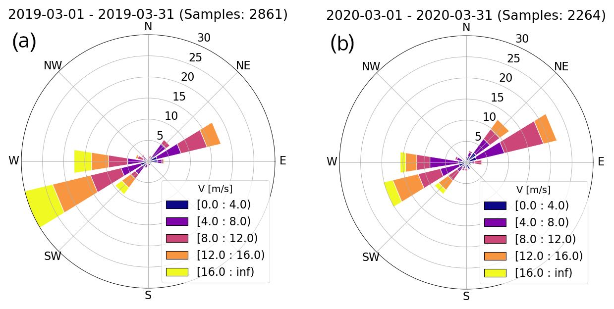
Figure 2Wind rose plots showing the wind speed and direction distribution for March 2019 (a) and 2020 (b) at an altitude of 874 m. The measurement data are retrieved from a nearby wind profiler (47.69∘ N, 8.62∘ W) in the district of Schaffhausen. The altitude of the wind measurements is comparable to the altitude of the nacelles of the wind turbines, and the horizontal distance to the turbines is about 8.8 km. The colors indicate the wind speed intervals in a bin width of 4 m s−1.
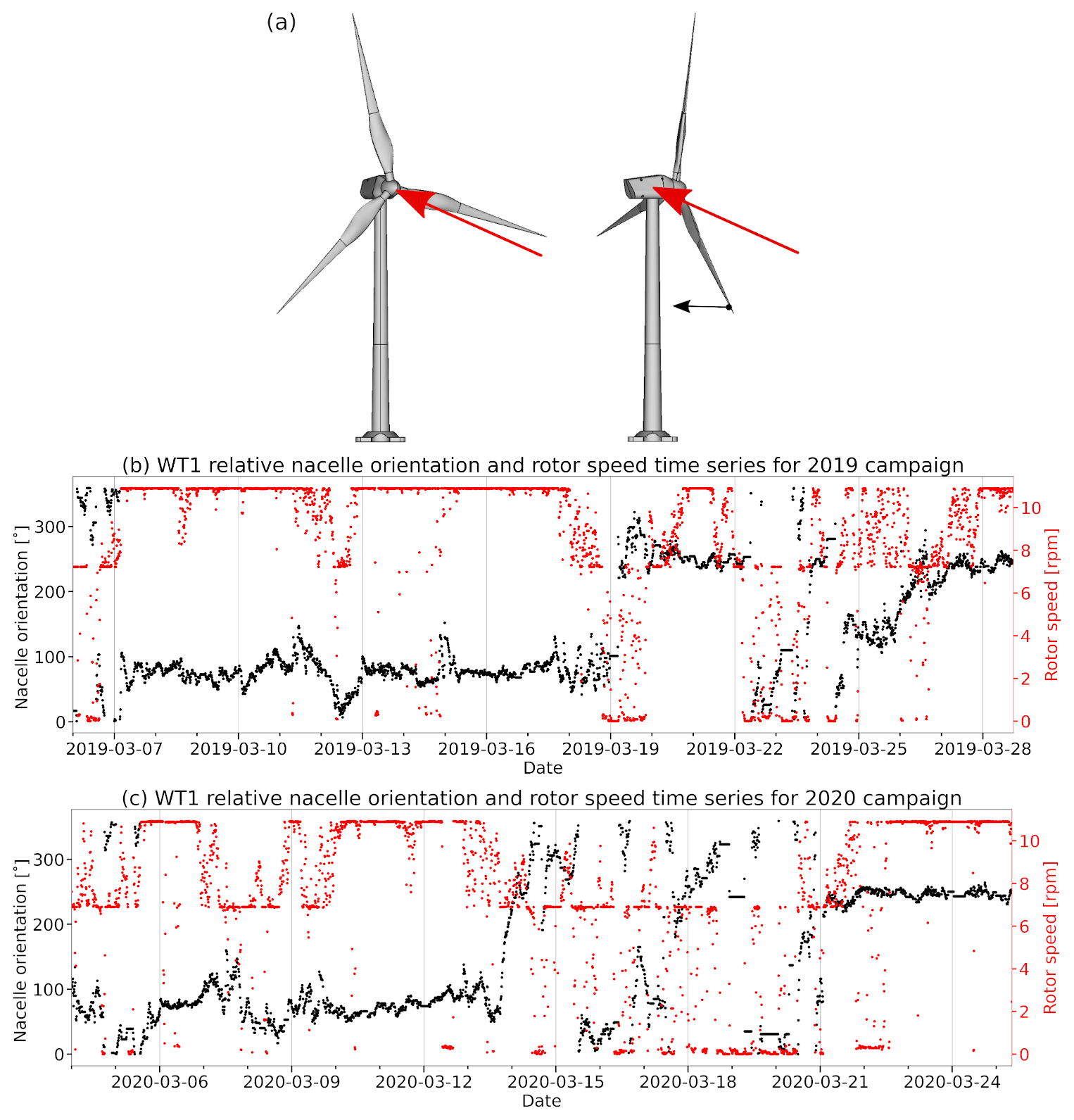
Figure 3In (a) a schematic view of two wind turbines in relative nacelle positions of 0∘ (left) and 270∘ (right) with respect to the radar angle of attack (red arrows) is shown. The blade pitch angles are at a high position (), and the direction of blade bending during wind load is indicated by the black arrow. The plots (b) and (c) show the time series of relative orientations (black), with respect to the radar location, of the WT1 nacelle from 6 to 28 March 2019 and from 4 to 25 March 2020. On top and specified by a secondary y axis, the associated rotor speeds are presented in red, in revolutions per minute (rpm). For the measurement campaign in 2019 the time series plot is representatively shown for wind turbine WT1. The offset angle between relative and absolute nacelle orientations is 158.9∘.
In order to illustrate the narrow-sector PPI scans of the weather radar in 2019, the four plots in Fig. 4a–d are shown. At an elevation of 3∘ PPIs of the horizontal reflectivity ZH (a), the differential reflectivity ZDR (b), the co-polar correlation coefficient ρHV (c) and the Doppler spectrum width W (d) are represented on 24 March 2019. The wind turbine clutter is made visible by the black 35 dBZ reflectivity contours in all shown PPI moment data at the range from 7.7 to 8.6 km. The impact of turbine clutter cannot be seen in all PPIs clearly. While ZH shows values up to 40–50 dBZ for the given elevation of 3∘, ZDR attains mostly slightly negative numbers within the 35 dBZ contours. In those areas and in the shadow behind, ρHV is reduced to approximately 0.7 compared to the hill forest clutter in front of the wind turbines, where ρHV reaches more than 0.95. For this specific example and the slow PPI scan, the Doppler spectrum width remains close to 0 m s−1 on average as indicated by the violet areas.
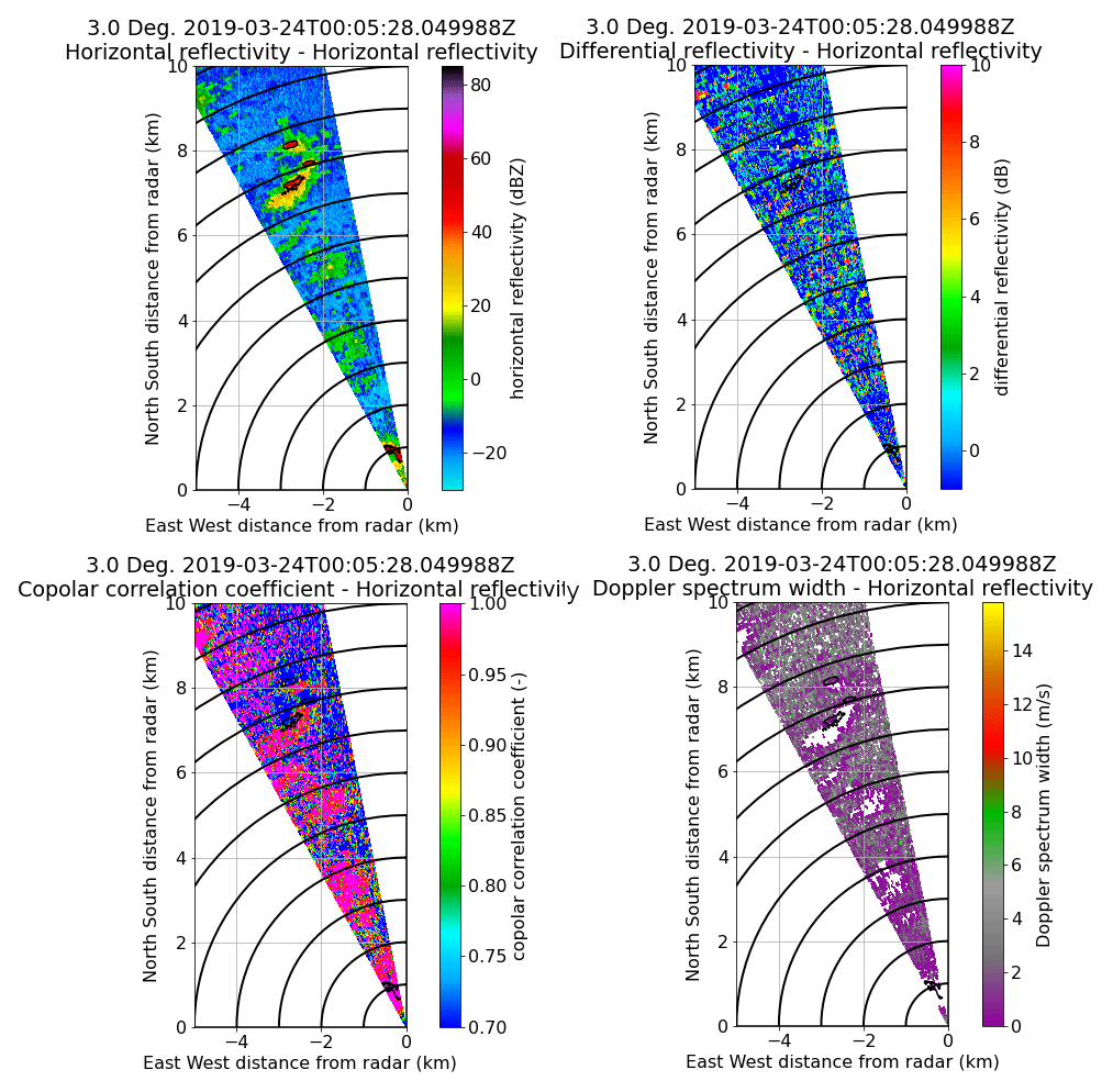
Figure 4Example of single PPI slices (a–d) of horizontal reflectivity ZH, differential reflectivity ZDR, co-polar correlation coefficient ρHV and Doppler spectrum width W covering the wind park of the three wind turbines at an elevation angle of 3∘ on 24 March 2019. The black circles indicate a range spacing of 1 km. In all PPI slices the 35 dBZ reflectivity contour is drawn to show the approximate location of the three wind turbine scatterers.
For the statistical analyses, azimuth elevation plots at a fixed range or range span are used. Figure 5a–d show for a specific PPI (a) and RHI (c) scan sequence the maximum horizontal reflectivity within the range span of all the three wind turbines. Below 2∘ in elevation, a software-based blanking was applied to the radiation transmitter for safety reasons. All three wind turbines can be distinguished in these kinds of plots. WT1 (left signatures at 339∘), with the best visibility, has in this example the highest returns, of about 60 dBZ within the center region, where the nacelle is located. The benefit of the RHI-based results is the larger overview for elevations up to 10∘. Figure 5b and d show the range gates from both scan sequences, respectively, where the maximum of ZH occurred. With the distance of these range gates, it is obvious that the high returns left of WT1 are not associated with a turbine effect as they appear at a shorter distance from the radar, of about 7500 m, compared to the WT1 distance of 7740 m. Given the surroundings consisting of uphill terrain (see Fig. 1), the high radar returns most likely have their origin in background clutter from the hill forests.
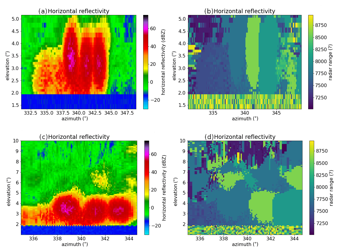
Figure 5Fixed-range span plots of the maximum retrieved horizontal reflectivity ZH from the PPI (a) and RHI (c) scan sequences are shown. The axes indicate the azimuth and elevation angles. The subplots (b) and (d) show the range gates from both scan sequences, respectively, where the maximum ZH occurred. Be aware that azimuth and elevation span is different for the PPI- and RHI-based fixed-range span plots. The former go from 331 to 349∘ in azimuth and from 2 to 5.1∘ in elevation and the latter from 335 to 344.6∘ in azimuth and from 2 to 10∘ in elevation.
In March 2020 the radar was placed exactly at the same location as the year before. The whole campaign lasted 22 d and was dedicated solely to the observation of wind turbine WT1. The radar beam center was targeted at the elevation of the nacelle and thus towards the center of the rotors. The detailed characteristics are summarized in Table 4. In total we gathered 2.429×10⁷ data samples, where one sample (or one radial) consists of 128 averaged radar pulses. The full ZH data set is illustrated also later in Sect. 3.1 with Fig. 8. Together with the available environmental wind turbine data, which are available at a 10 min resolution scale, we aim to find relations for the occurrence of radar return maxima and minima as well as their variability.
In the following part of the paper, all the horizontal reflectivity ZH measurements obtained from PPI and RHI scans in 2019 are statistically analyzed in order to characterize the returns from the three wind turbines by using the radar data processing framework Pyrad (Figueras i Ventura et al., 2020a). Global statistics considering the median and maximum ZH are presented. Given the stability of the location of the wind turbine signals, statistics can be computed at fixed ranges on a two-dimensional plane that is given by azimuth (x axis) and elevation (y axis) (see Sect. 3.1). While radar reflectivity values may be informative, a core piece of information allowing the generalization of the measurements collected is the retrieved RCS, usually given in dBsm (dB square meters). Its added value with respect to reflectivity alone is that it is a pure property of the target. The RCS values that are shown here are retrieved from the inversion of the formula for the radar reflectivity Z. According to Battan (1973) the radar equation for a single, isolated target is
where [pr]=mW is the received lossless power by a directional antenna.
The log-transformed power can be derived by , where p0=1 mW. In Eq. (1), the backscattering cross-section or RCS is indicated as σb (assuming a monostatic radar with a scattering angle of for the angular RCS), the antenna gain as , the radar wavelength as λ and the transmitted power as pt; θH and θV are the horizontal and vertical beam widths in radians. Usually σb is expressed as a scalar, and the dependencies on wavelength are implicitly assumed: in our case λ=0.032 m. [σb]=m2 and, respectively, , where σ0=1 m2.
Precipitation particles act as distributed scatterers in the volume of air illuminated by the weather radar. The resolution volume Vr filled by a transmitted pulse can be approximated by a cylindrical shape, given the radar pulse width τ and the range r:
Accounting for the actual distribution of power within the beam generated by a parabolic antenna, a correction factor of was introduced by Probert-Jones (1962):
The backscattered signal from a volume of randomly distributed scatterers is the sum over all scattered signals. The summation of the backscattered cross-sections from precipitation scatterers in a unit volume is called the radar reflectivity and is defined as . The final form of the radar equation for distributed scatterers, like precipitation, combines Eqs. (1) and (3) and substitutes z in the resolution volume, , for σb,i. The general form of the radar equation that is valid for scatterers of all sizes yields
The general assumption behind the formulation presented in Eq. (4) is that of a pulse volume homogeneously filled by a huge number of randomly distributed backscatterers. For a weather radar, the average returned power has to be related to the physical characteristics of the particles within the resolution volume. The Rayleigh approximation of the backscattering cross-section of a single water drop σb,i can be expressed according to, e.g., Fabry (2015) or Ryzhkov and Zrnic (2019) as
where |K| is related to the complex index of refraction. By substituting Eq. (5) into Eq. (4), the radar equation for spherical drops can be written as
The conversion to the wind turbine radar cross-section σb that has been used in our study is finally shown by Eq. (7).
The three conversion values F, which have to be subtracted from the retrieved [Z]=dBZ to obtain [RCS]=dBsm for all wind turbines, are summarized in Table 5. The reflectivity in linear unit is given by (Bringi and Chandrasekar, 2001), where .
Table 5Conversion factors F to obtain the radar cross-section (RCS) from ZH for the three wind turbines WT1, WT2 and WT3.

With the much better temporally resolved measurements acquired in 2020 with the fixed-pointing scan mode of the weather radar, the impact of the turbine orientation, blade pitch angle θ, rotor speed rs and wind speed , as a measure of blade bending, on the retrieved horizontal reflectivities is investigated later in Sect. 3.2. In a first step, the relative turbine (nacelle) orientation is solely used to stratify the returns with an azimuth bin of 10∘ width. Then, in order to measure the strength and direction of possible relationships between the different WT data sets, we perform a correlation analysis based on the Pearson correlation coefficient. In order to simplify the use of a linear regression, we converted the relative nacelle positions α to normalized positions Ψ such that values between 0 and 1 map symmetrically and independently between backward- or forward- and sideways-facing of the WT nacelle. We calculate Ψ simply as Ψ=|sin α|. For clarification, a Ψ value of 0 means that the turbine's angle of attack is facing either towards the radar or away from the radar, while a value of 1 shows the sideways case, when the angle of attack is perpendicular to the radar beam. With the Ψ parameter, a more reasonable calculation of the linear Pearson correlation coefficient is achievable because the polar 360∘ projection of the turbine position alone has a symmetry.
3.1 Global statistics of horizontal reflectivity ZH and radar cross-section (RCS)
The global statistics are computed at a range distance of 7740 m (WT1), 8040 m (WT2) and 8600 m (WT3) over the entire data set of the 2019 field campaign. The statistical overviews in Figs. 6 and 7 show the maximum (first row) and median (second row) of ZH for all three wind turbines. The used data set to compute the statistics for Fig. 6 refers to all PPI scans, while for Fig. 7 all RHI scans were processed. As can be seen in those images, the visibility over the wind turbines was very good for the selected site. At elevation angles lower than 2∘, sector blanking has been applied, where the radar transmission was turned off for safety reasons. While the elevation span of the PPI scans is enough to fully observe the wind turbines, the increased vertical span of the RHI scans allowed the observation of the returns that are not associated with the main lobes of the radar antenna.
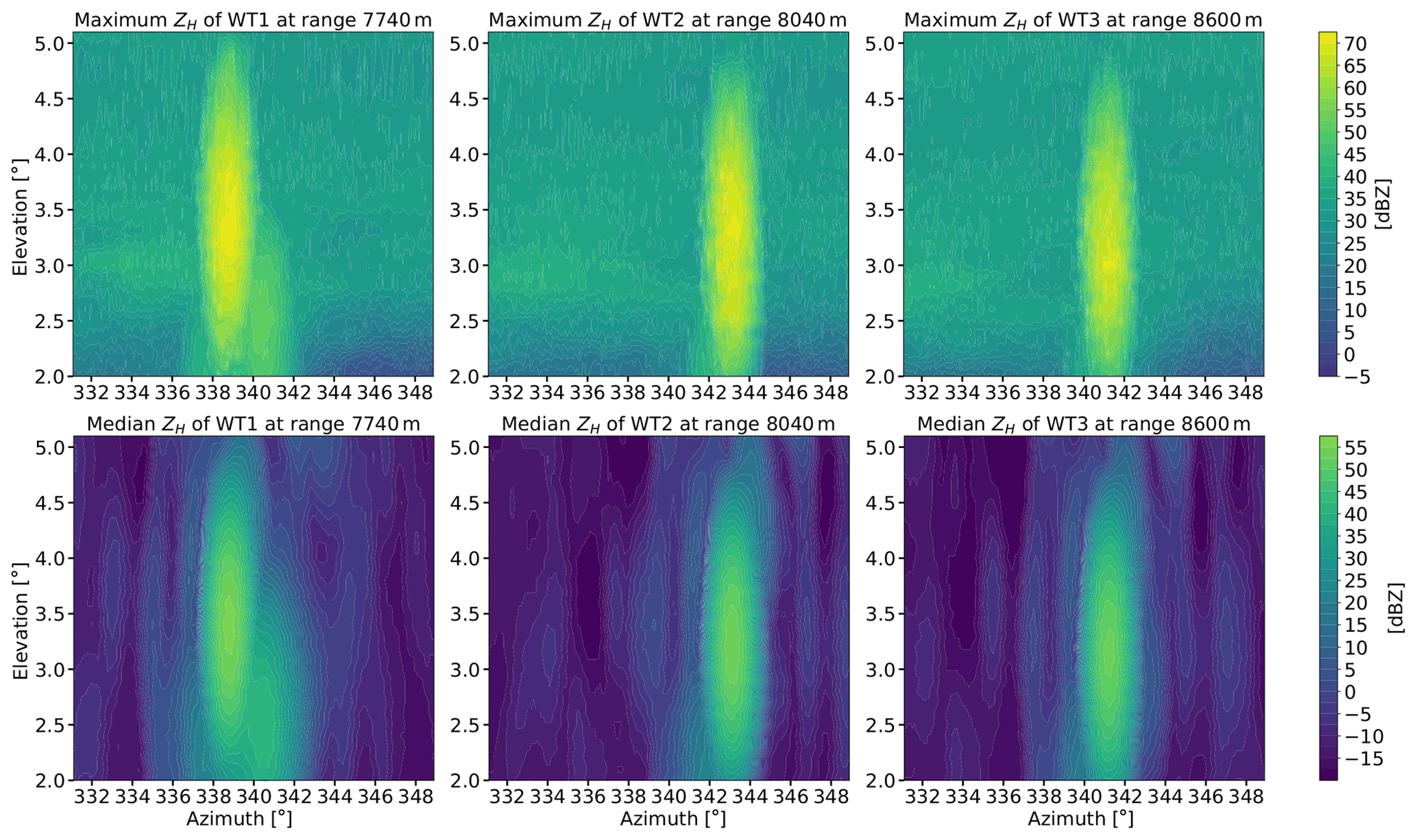
Figure 6Maximum (first row) and median (second row) fixed-range statistics from PPI radar scan data of horizontal reflectivity ZH for all three observed wind turbines during the entire measurement campaign in March 2019. The first column shows the results for WT1 (range: 7740 m), the second column the results for WT2 (range: 8040 m) and the third column the results for WT3 (range: 8600 m). The elevation angles go up to 5.1∘, and the azimuth range is 18∘ (see Table 3).

Figure 7Maximum (first row) and median (second row) fixed-range statistics from RHI radar scan data of horizontal reflectivity ZH for all three observed wind turbines during the entire measurement campaign in March 2019. The first column shows the results for WT1 (range: 7740 m), the second column the results for WT2 (range: 8040 m) and the third column the results for WT3 (range: 8600 m). The elevation angles go up to 10∘, and the azimuth range is 9.6∘ (see Table 3).
A clear example can be seen in the median value of ZH within Fig. 6. Secondary returns appear in the area surrounding the core of the wind turbines, either generating the visual effect of a ring signature around the most intense echoes or as secondary and tertiary replications of the intense signals. Those returns are 20 to 50 dB lower than the strongest returns from the turbines themselves. These signals remain significant and populate a large sector of azimuth and elevation angles around the actual location of the wind turbines, thus extending the area which has to be seen as WT clutter-contaminated. The characteristics of secondary or tertiary returns obviously depend on the characteristics of the antenna (shape, secondary lobes, symmetric or anisotropic behavior) of each individual radar.
Based on Fig. 6, we find the largest area of maximum returns (ZH) spreading from the rotor center of wind turbine WT1, which is likely related to the visibility of the radar beam. Regarding ZH, WT1 also reached the maximum of about 75 dBZ in the RHI data during the first campaign in 2019. By looking to the fixed-range contour plots of WT1, a very high and stable return signal can be identified to the lower right, at about 341∘ in azimuth and 2.5∘ in elevation direction. So far this signal could not be assigned to a source. Multi-path effects could be a possibility. By looking at the range gates in Fig. 4d it is evident that this peculiar signal has its maximum at the same range as the wind turbine WT1 and is thus likely related to the interference with this turbine.
While the location of the intense signals is stable in time, the intensity of the returns varies significantly. This is evident when we look at the differences between the maximum and median ZH values, which are on the order of 20 dB. One of the main objectives of the measurement campaign is the evaluation of the most critical scenarios in terms of high wind turbine radar cross-sections. Here we summarize the highest observed values and their frequency of occurrence. The highest RCS values retrieved were on the order of 40 dBsm for the RHI-based data set and 38 dBsm for the PPI-based one. These high values were very rare to observe; only a few echo counts could be assigned to them. WT1, with the best radar visibility, reached the highest values. The variability in the intensity of the maximum returns was found to be significant, and the maximum RCS of each radar scan can be as low as 20 dBsm (or lower). The underlying dynamics is given by the combination of the changing turbine orientation, motion of the rotors and blade pitch angles together with the motion of the radar antenna, which scans over the wind park and thus only covers the same exact spot at intervals of several minutes. This was the main motivation to introduce fixed-pointing observations during the second field campaign in 2020. The number of data produced with the fixed-pointing acquisition mode was as high as one radial collected every 64 ms. This increases the confidence that actual maxima of the radar returns are captured within our long dedicated observation period towards WT1. In order to give an idea about the number of data that were captured, the scatterplot in Fig. 8a is visualized, showing the whole time series of ZH (in black) and the corresponding 10 min moving median values (in red).
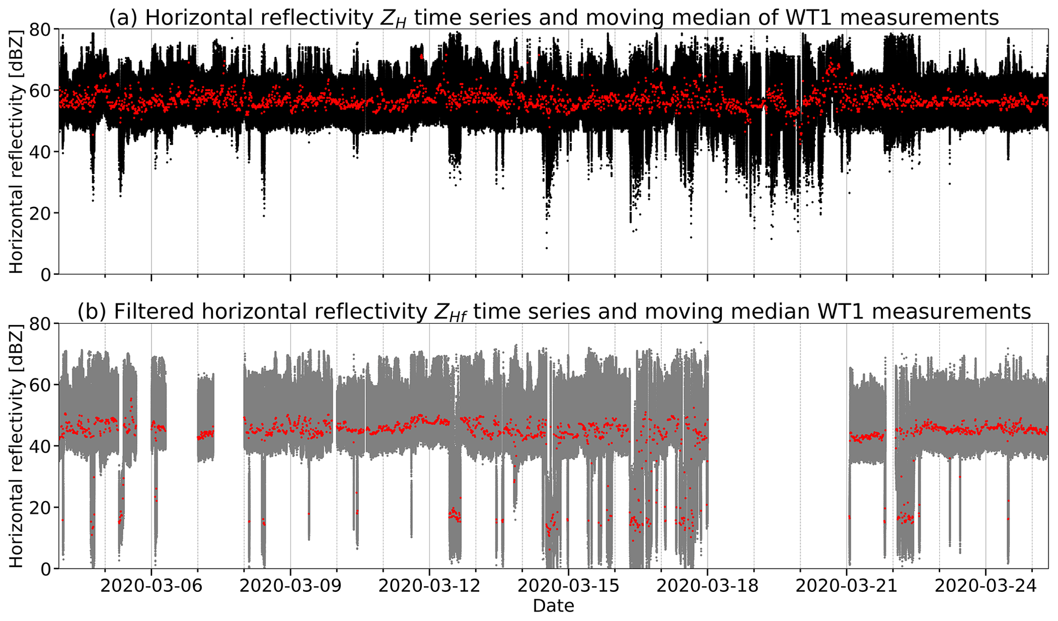
Figure 8In (a), the scatterplot time series (black dots) of horizontal reflectivity ZH values retrieved from wind turbine WT1 during the stare-mode measurements of the mobile weather radar in March 2020 (4 to 25 March 2020). The red colored line represents the corresponding moving median of the reflectivity data with a temporal window size of 10 min. In (b), the scatterplot time series (gray dots) of the clutter notch Doppler-filtered ZHf values and corresponding moving median. The clutter filter used has a width of 7 m s−1 and was applied during postprocessing to moment data where spectral data were available. In consequence, gaps appear in the time series of ZHf.
The variability in the returns remains extremely high, with typical short-term spans on the order of 20 dB. A first conclusion is that the variability which has been observed during the 2019 field campaign was not caused by the scanning strategy itself. With the radar stare mode, frequently higher maxima than during the PPI and RHI scans of 2019 were observed in the reflectivity data. Thus the usage of fixed-pointing data acquisition indeed improved the sampling of the right tail of the distribution of ZH values. This is especially important when worst-case scenarios are of interest, e.g., for aviation safety issues. ZH maxima of 78.5 dBZ (equivalent to an RCS of 44 dBsm), about 4 dB higher than what has been observed in 2019, were measured. From the time series shown in Fig. 8 some interesting periods can be identified when the spread between the maxima and minima of ZH suddenly increases. Between 14 and 21 March 2020 such sudden increases were more frequently observed. In Sect. 3.2 we investigate these findings in depth by performing correlation analyses with, i.a., the pitch angle θ of the rotor blades. The 10 min moving median mostly stays between 50 and 60 dB over the 2020 campaign period, occasionally going up to 65–70 dB.
Having access to spectral data, it is worth investigating the potential of frequency-domain filters to suppress the returns of the wind turbines. Thus, we tested a spectral clutter suppression of 7 m s−1 width (suppressing the returns in the Doppler interval ). The spectral clutter suppression shown here is simple: the contribution of power corresponding to the Doppler velocities within the width is removed. Data collected in 2020 allow for a finer comparison of filtered (clutter-suppressed) ZHf data and unfiltered ones. First, it can be observed how the operational characteristics of WT1 affect the efficiency of clutter removal. And second, the corresponding removal of static parts like the WT tower and mostly the nacelle allows the assignment of the seen effects in the radar returns to the remaining moving rotor blades.
Doppler spectra have been collected every 5 min for 5 min during the field campaign in 2020, with a few days of data gaps given by the very high demand in terms of data computation and transfer on the signal processor. However, we can get a clear idea of how a clutter-notch-based filter performed during the entire campaign (see Fig. 8b). The clutter suppression is very efficient as soon as the rotor speeds get close to 0 rpm, and most of the signal can be removed. The median residual reflectivity is on the order of 20 dBZ in those cases. The zero-Doppler component of the wind turbines is very high even when the turbine is spinning. In this way, the clutter notch filter can remove a part of the signal even during normal operation of WT1. Looking at the plots, this reduction is on the order of 10 dB in median terms. Overall this is a significant attenuation, but one must keep in mind that the residual signal is still very high.
3.2 Impact of WT orientation, blade pitch angle, rotor speed and wind speed on ZH
Given the availability of the WT and wind sensor data, it is possible to perform turbine orientation stratified statistics with ZH and ZHf. The first experiment, which was conducted in 2019, provided non-conclusive results with respect to the orientation of the wind turbines, and this was another reason that motivated a second experiment in 2020. Now, with the high-temporal-resolution data, we are more confident about the obtained results that we intend to show here. Both March 2019 and March 2020 had similar statistical meteorological wind patterns (see Fig. 2), which led to comparable distributions of the relative nacelle orientations (see Figs. 3b and 3c). A different view of the relative positions is provided in Fig. 9, where the normalized polar distribution is shown in combination with the rotor speeds for the ZH and, respectively, ZHf data. To briefly clarify the relative nacelle positions, a value of 0∘ means that the long axis of the rotor blades is perpendicularly aligned to the direction of the radar beam center, and the WT is pointing towards the radar (left WT schematic in Fig. 3a). In contrast, a value of 180∘ represents a WT pointing away from the radar, and with the long axis of the blades is aligned parallel to the center of the radar beam (right WT schematic in Fig. 3a).
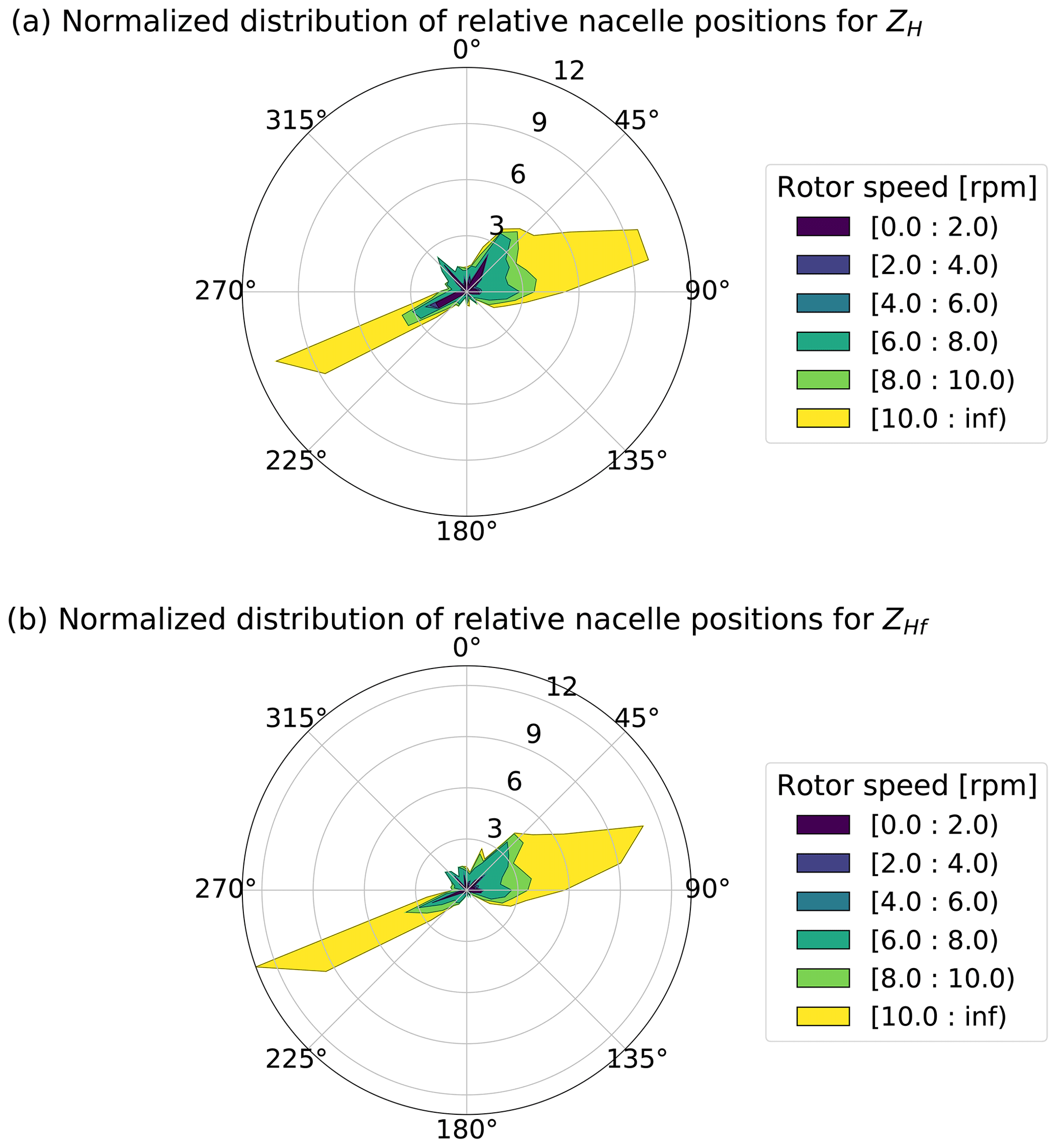
Figure 9The plots indicate the normalized distribution of relative nacelle positions with corresponding rotor speeds during March 2020 for the unfiltered ZH (a) and filtered ZHf (b) reflectivity data. The rotor speeds are binned with a width of 2 rpm.
From the polar plots in Fig. 10a we see that the maximum measured reflectivities are insensitive to the relative yaw angle of the nacelle. This is evident by the round and not too much disturbed distributions (less than 10 dB) of the color-mapped scatter points. In this plot the maximum ZH values are counted within a bin width of 0.5 dB. Biased by the wind direction distribution in March 2020, most maxima were retrieved at 270∘, marked by the yellow scatter point, with a total number of 10 data values. By having a look at the 99th percentile distributions together with the number of counts exceeding the plotted values of the scatter points (inner color-mapped scatterplot circle), first deformations of the distribution in the polar plots become visible and even more in the median distribution (red scatter points). It is interesting to observe how, in median terms, the relative orientations near 180∘ are associated with higher returns, while for 99 % quantiles, similar signals are observed also at orientations near 90 and 270∘.
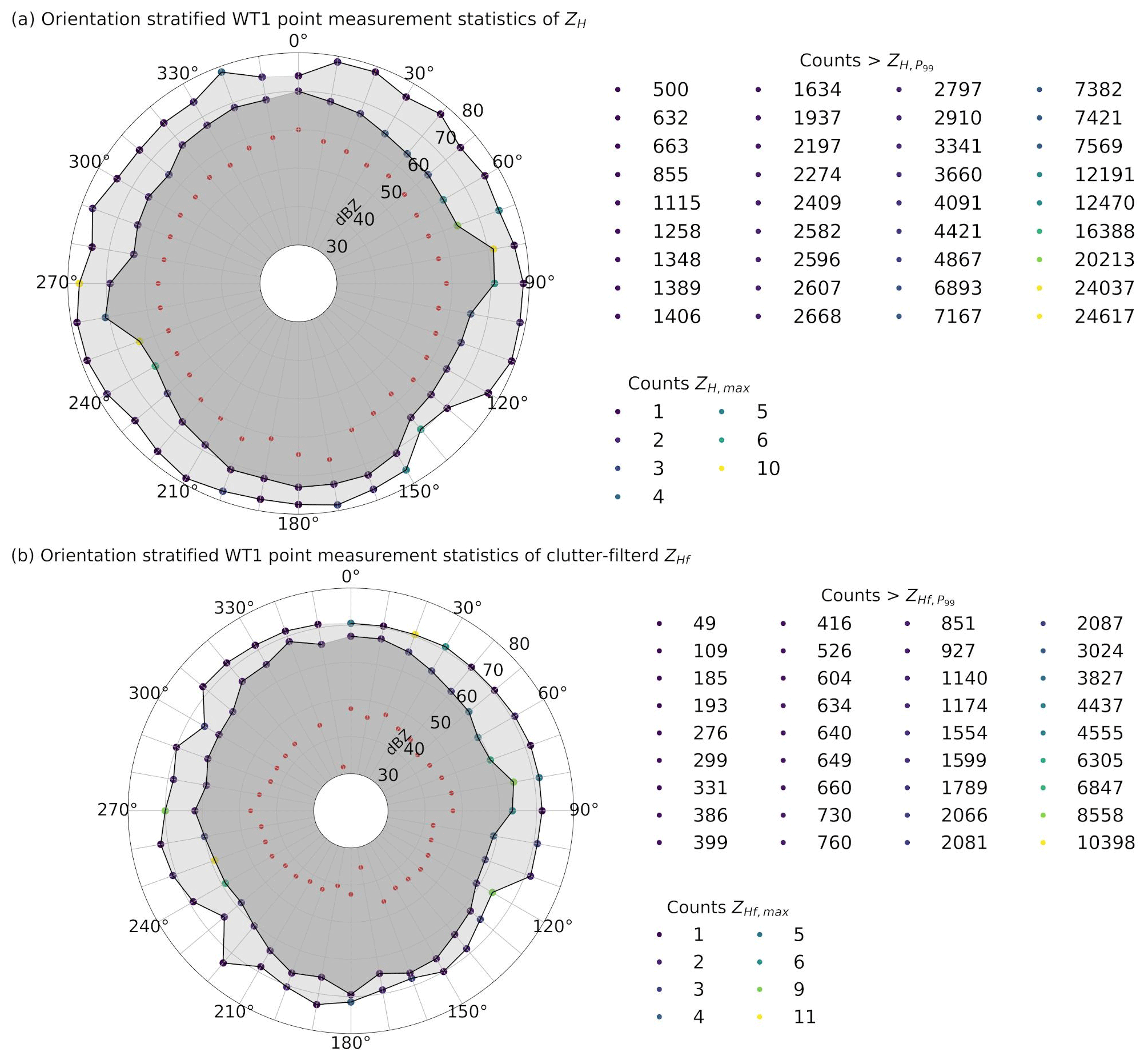
Figure 10Fixed-pointing measurement statistics of horizontal reflectivity ZH (a) and clutter-filtered ZHf (b) based on the relative position of the WT1 nacelle. The median value is indicated by the red scatter points in all polar projections. The maximum values with the corresponding counts within a bin width of 0.5 dB are shown by the light-gray shaded area and color-coded scatter points. The dark shaded area represents the results for the 99th percentiles, with the counts exceeding them indicated by the corresponding color table.
With Fig. 10b (ZHf data only) in comparison, we try to separate the effects of the moving parts, which is mainly the rotor blades, from the static returns from the tower and nacelle. We assume that the returns from the slow-moving nacelle are significantly reduced by the applied filter. In the polar distribution we find that the maximum ZHf values get reduced by 5–10 dB and reach mostly around 70 dBZ, still rather independent of the relative WT1 orientation. The median distribution for ZHf drops remarkably at two positions, 170 and 350∘. But this result is statistically not significant as the data samples for those directions are in general small (below 2 %) and further decreased for the filtered reflectivity data (see Fig. 9b). A higher reduction (>10 dB) is found at 260∘ for the 99th percentile when the turbine is pointing rightwards (wind direction from the east) but not for the opposite direction (WT pointing leftwards). One explanation can be that the radar beam center is filled with more moving parts of the turbine when the WT is pointing leftwards. This could be the case when the moving rotors are spinning in front of the field of view towards the tower or nacelle.
Figure 11 compares on a 10 min moving window the maximum, minimum and median of filtered and unfiltered reflectivity. The separation of the individually colored scatter points indicates the two modes of the turbine, moving and not or only slowly moving. As naturally expected, the filter is more efficient when WT1 is not or is slowly moving. The fact that the difference between ZH,max and ZHf,max is smaller than the difference in the median or minimum is an additional sign that the high ZH comes preferably from the moving WT parts. Regarding the possible influence of the WT nacelle, it can be argued that the effective scattering area of the WT nacelle is small compared to the area of the rotor. In the end this could lead to a stealth behavior as long as the radar angle of attack is not perpendicular to the nacelle surface, which is given for our measurement setup. Future work should also take into account numerical simulations to assess the complex interactions in more detail.
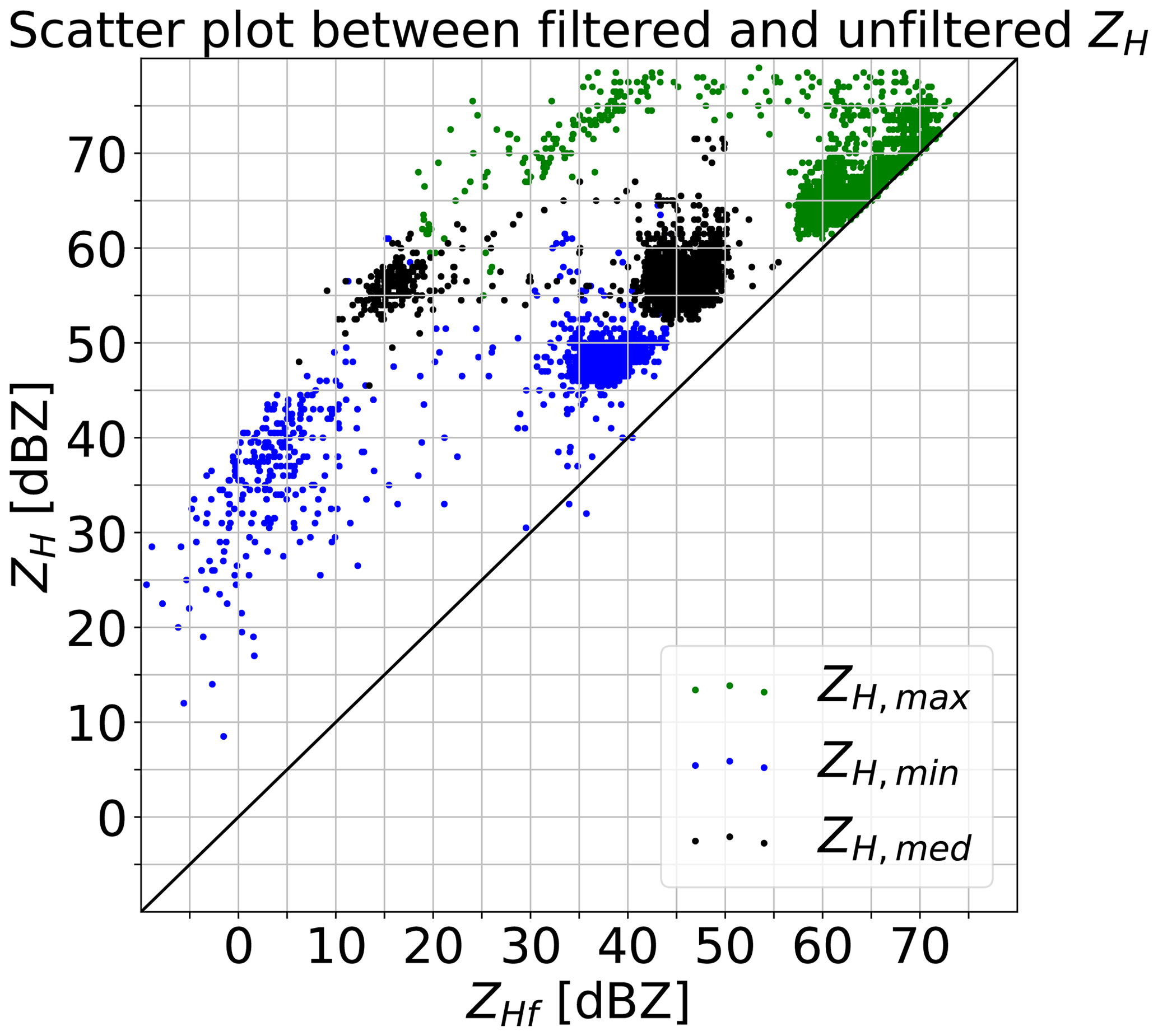
Figure 11Scatterplot comparison of 10 min moving minimum (blue), maximum (green) and median (black) ZHf from Doppler-filtered (clutter notch of ) and unfiltered reflectivity data ZH.
The complexity of an operating wind turbine is related not only to the nacelle and, respectively, the rotor orientation (yaw angle) but also to the varying blade pitch angles θ, which are used to control the rotor speed (power production) when the wind speed is changing. The profile of the blade rotates along the axis from the hub to the blade tip in order to maintain the angle of attack (Gipe, 2004). θ is a parameter that may vary at the timescale of seconds. Unfortunately, the granularity of the available wind turbine data (10 min resolution) does not allow us to match the observed maxima with the actual wind turbine parameters at the exact same time, but while looking at how the maxima and minima appear in the data (see Fig. 12a) it is reasonable to assume that the blade angle is a key parameter. From the time series plots themselves, a linkage between the blade angles and moving ZH,max (green line) and ZH,min (blue line) signatures is obviously present during certain time periods. For example on 12 or 22 March 2020, blade pitch angles of WT1 were aligned at roughly 90∘ over hours, and at the same time the maximum ZH values increased by more than 10 dBZ accompanied by a heavy increase in the spread between the minima and the maxima, which is equivalent to an increase in the overall variability. It can be concluded that large changes in the blade angles over time, like in the time period between 16 and 21 March 2020, lead to a strongly increased variability in the captured radar returns.

Figure 12The line plots in (a) show the 10 min moving maximum (green) and minimum (blue) of [ZH]=dBZ as presented in Fig. 8. The black (rs≥1 rpm) and red (rs<1 rpm) scatterplots indicate the WT1 blade angles with a temporal resolution of 10 min. The time period between 4 and 25 March 2020 covers the whole 2020 field campaign. For practical reasons, plot (b) presents the relative nacelle orientation according to plot (a).
Another, unfortunately unsupervised, WT parameter which is supposed to influence the results is the bending or deflection of the blades, occasionally enhancing the radar returns. Realistic simulations by Zhang et al. (2018) assumed blade mid-deflection angles of 15∘ for a 37 m blade length. Converted to larger turbines, like the Nordex SE N131, with blades as long as 65.5 m, bending distances of 17.15 m at the blade tip level result if the deflection angle reaches 15∘. The signal enhancements are possible even if the wind turbine is not pointing towards the radar as the blades are twisted, and therefore mirror effects are even possible sideways in azimuth and, respectively, elevation from the main orientation of the rotational axis of the rotor. The blade bending effect is naturally closely related to the wind and rotor speed. The coupling between the bending and torsional deflection of a blade is generally known as aero-elastic tailoring (Weisshaar, 1981).
From the viewpoint of a megawatt-class turbine operator the stability of power production is important when delivering electricity into the grid. When the wind conditions are not good enough (e.g., too low wind speeds), and stable power production cannot be assured anymore, the wind turbine is put into a so-called sailing position. In such a position the pitch angle of the blades θ is highly increased () compared to normal operation, allowing the rotor to slowly turn (usually below 1 rpm) while keeping the bearings of the system greased. Further, the axial turbine load is constantly varying, which is also important to reduce the mechanical stress. During certain, mostly rare time periods, θ is put over 90∘ to aerodynamically break the rotors. Possible reasons are temporal fast-changing gusts of wind, for instance during thunderstorm activity, or an external slowdown triggering to reduce fatalities, i.e., of birds and bats.
Next, a Pearson-based correlation analysis between the WT1 operation data and the radar returns is presented for the fixed-pointing measurements of 2020. One idea was to oppose the correlation results with data during a normal (power production) and abnormal (breaking or sailing) wind turbine operation. Therefore a threshold of 1 rpm for the rotor speed has been chosen to sub-divide the resampled (10 min) data sets of horizontal reflectivity (ZH,max, ZH,min, ZH,r, ZH,med) and WT parameters (θ, Ψ, rs, ). For the moving maximum ZH,max (green line in Fig. 12a) and the pitch angle, a weak positive Pearson coefficient r of 0.32 resulted. More interesting is the result between the moving minimum ZH,min (blue line in Fig. 12a) and θ.
A theoretically strong downhill linear relationship with can be calculated for them, but it has to be taken into account that the complex blade surfaces will likely not give a linear radar echo response, which in turn would initiate some misleading result. In addition the abnormal turbine modes with less variable blade angles bias these results further. By only taking into account the data where rs≥1 rpm, the correlation coefficient is reduced to −0.56. For ZH,max in contrast the change is small, with r reaching 0.34. The corresponding correlation heat maps for both WT modes, separated by the defined rotor speed threshold of 1 rpm, are presented in Fig. 13.
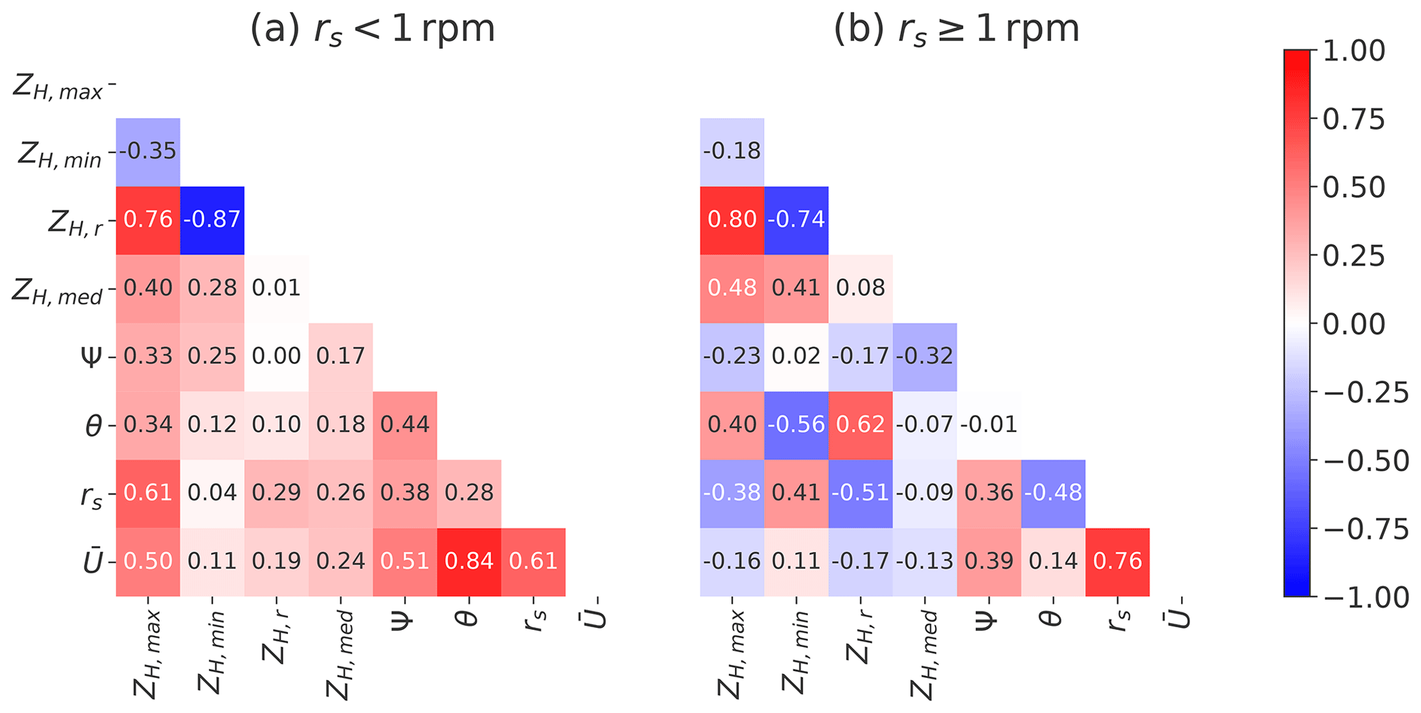
Figure 13Pearson linear correlation coefficient heat map matrices between radar returns, resampled to a temporal resolution of 10 min (maximum ZH,max, minimum ZH,min, difference ZH,r, median ZH,med) and WT1 orientation Ψ, blade pitch angle θ, rotor speed rs and average wind speed . The correlation matrix (a) is computed with the measurements when the rotor speed rs is less than 1 rpm and (b) when rs is equal to or higher than 1 rpm. Some corresponding regression line fits are shown in the scatterplots of Fig. 14.
Furthermore, strong uphill (positive) linear relations can be found between the rotor speed and the moving minimum ZH,min (r=0.63) for all of the data and between the blade pitch angle θ and the difference ZH,r (r=0.64) between the min and max values. From this point of view we deduce that θ is a good measure for the observed variability in the horizontal reflectivity of a wind turbine. Naturally, the rotor speed rs and θ have a very high anti-correlation (), and further it is interesting to see that without sub-dividing the data sets no significant relevant linear relation is evident between the ZH data sets (including the 99.9 and 0.1 % quantiles) and Ψ (simplified relative nacelle orientation) or average wind speed (measure of blade bending). By looking at the rs threshold split correlation heat maps in Fig. 13a and b, this picture changes. For the rs<1 rpm case, Ψ now has a low positive correlation towards the maximum returns (r=0.33), and the coefficients for even reach 0.5 (moderate uphill linear relation) when the turbine is in sailing or aero-breaking mode. On the other hand the ZH,r loses the high correlation towards the pitch angle when the rotor is only slowly idling with the wind. This can be explained by the fact that θ is not adjusted much during these abnormal operation modes as is evident in the scatterplot of Fig. 14a (vertically aligned scatter points for rs<1 rpm). In more detail the plots in Fig. 14 show four different color-coded scatterplots between the blade pitch angle θ or normalized relative yaw angle Ψ and ZH,max and ZH,min, respectively, below and above the rotor speed threshold of 1 rpm. In addition, the linear regression lines with confidence interval sizes of 95 % for the regression estimate are drawn using translucent bands around the regression line. The maximum returns increase as the blade pitch θ increases, and this is especially true when the turbine rotors rotate slowly (sailing mode). We also see a high variability in ZH,min when θ is roughly at 70∘ or 90∘ (rs<1 rpm). A positive correlation of ZH,max and negative correlation of ZH,min could be identified when the wind turbine is in normal operation mode. Given the possibility that ZH,max is facing some radar saturation issue during the 2020 measurement campaign, it could be the case that the correlation coefficients are lower than they should be.
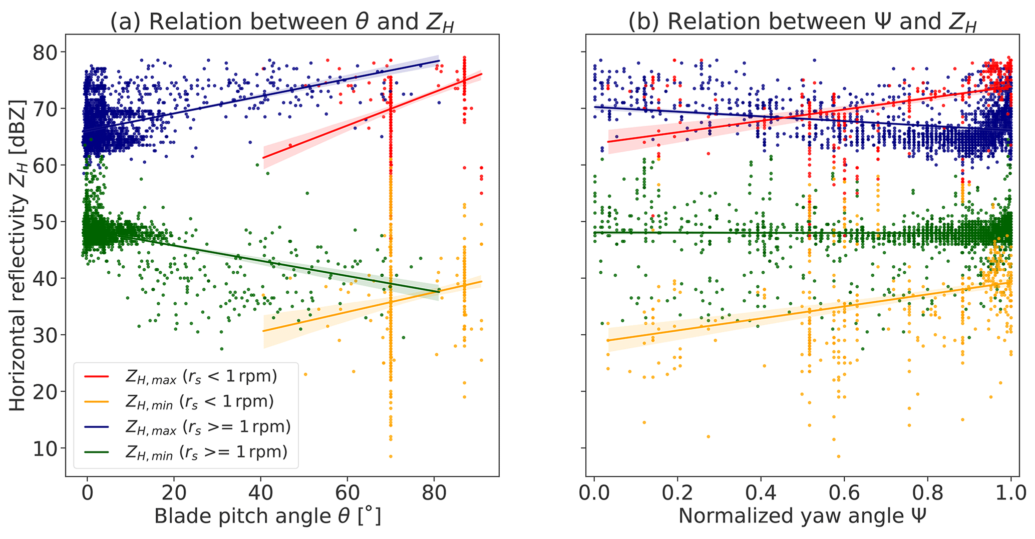
Figure 14Scatterplots and corresponding linear regression lines with confidence interval sizes of 95 % for the regression estimate (translucent bands) showing the relations between the blade pitch angle θ (a) and normalized nacelle orientation Ψ (b), respectively, and different sub-data sets of ZH. In particular the data sets ZH,max (blue and red) and ZH,min (orange and green) are each separated for the WT1 rotor speed threshold of 1 rpm. The confidence intervals are estimated using a bootstrap method.
One question that arises is what is causing the high variability in the minimum and maximum radar returns when θ is nearly constant (yellow and red scatter points in Fig. 14a). The remaining WT parameters are the nacelle orientation and possibly the blade bending related to the wind force. Both parameters are investigated in more detail with the help of Figs. 14b and 15. By investigating the ZH relations towards Ψ, the positive Pearson correlation coefficient already presented is now visible by the regression lines for the data sets with rs<1 rpm (comparable color codes as for θ). It has to be added that a significant shift to stronger echoes is not described by the linear relation. Some part of the variability in the horizontal reflectivities during the abnormally slowly rotating turbine modes can be ascribed to changes in the azimuth pointing of the turbine (yaw angle), which in turn changes from the radar location point of view the backscatter efficiency of the blades when the pitch is constant. The fact that the radar observations were most of the time facing the WT from the side is clearly seen by the majority of scatter points beyond Ψ values of 0.8.
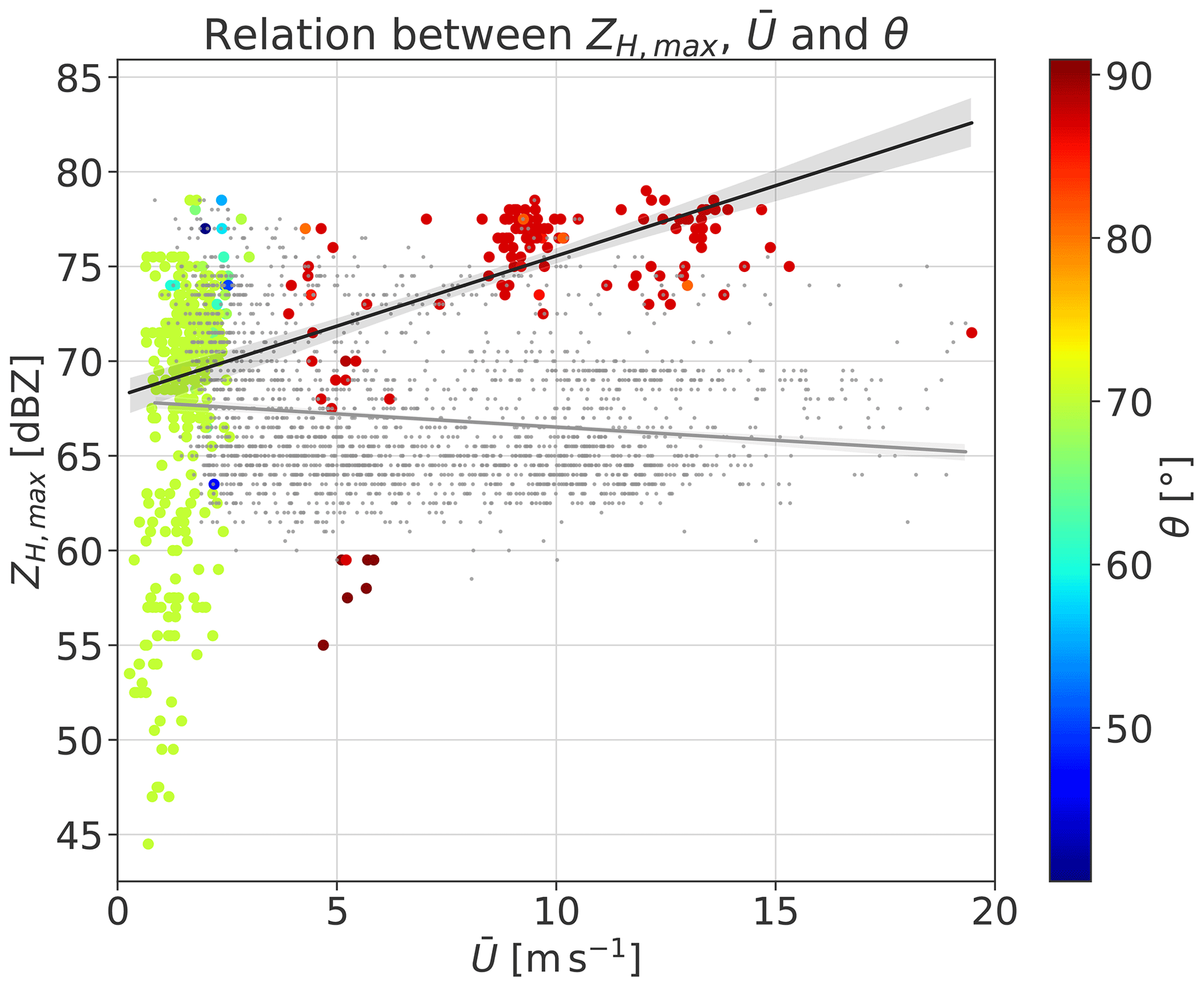
Figure 15Scatterplots and corresponding linear regression lines with confidence interval sizes of 95 % for the regression estimate (translucent bands) showing the relations between the average wind speed and two sub-data sets of ZH,max. The data when the rotor speed rs≥1 rpm are plotted in gray, while the data for rs<1 rpm are represented by the color-mapped scatter points. The color dimension shows the blade pitch angle θ. The black regression line belongs to the color-mapped scatter points. The confidence intervals are estimated using a bootstrap method.
The second, more fuzzy and thus difficult WT parameter to assess is the blade bending. One way to increase the transformation of wind energy into power is to produce and use longer blades without a large increase in weight. Such blades, which are in use nowadays, tend to be less stiff and will be more easily bent towards the tower with the wind load on it. Thus as a first guess, we assume that the blade bending is strongly related to the wind speed. In consequence we now try to find relations between ZH,max and by still keeping the blade pitch in mind. The information of all three variables is combined in the scatterplot of Fig. 15. The WT sailing mode with blade pitch angles close to 70∘ happens mostly when the average wind speed is basically below the cut-in wind speed of 3 m s−1, when the power production is not economic or even possible. Clusters of scatter points at high ZH,max are more likely accompanied by θ values of 90∘, when the average wind velocity is high. The fact that the turbine is still not going into normal operation during the high-wind-speed cases might be related to too strong and changing wind gusts, making stable electricity production difficult. For those cases we also find highly reduced variability in ZH,max.
When the WT is in normal mode (gray scatter points) no obvious linear relation between ZH,max and the wind speed is visible. In order to not overload the information given in the plot, the color-coded blade pitch dimension is only shown for the abnormal WT modes (rs<1 rpm). The tendency for higher ZH,max with increasing is perceivable and adds up to the positive correlation with the change in WT orientation Ψ.
In conclusion, complex interactions between θ, Ψ and should explain to a large extent the occurrence of the maximum returns as well as the overall captured variability. With this knowledge, statistical methods like OLS (ordinary least square) fits can be deployed to the data as introduced in the next Sect. 3.3.
3.3 Ordinary least square fitting to explain ZH,max variability
Here we briefly present the outcome of an ordinary least square model fit for the dependent variable ZH,max (2406 data samples) by using the independent wind turbine parameters θ and Ψ (Pearson ) during normal WT operation (rs≥1 rpm; Fig. 14b). The method should not be applied during the abnormal operation as θ and Ψ have a linear correlation (see Fig. 14a) and cannot be handled as independent variables anymore. For the computation we make use of the Python package scipy.stats, and for more details, also on OLS, we refer to Seabold and Perktold (2010).
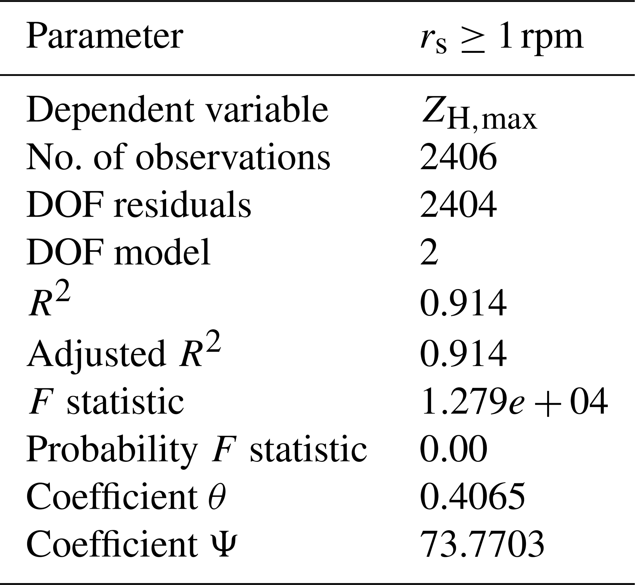
The key summary of the OLS model fit results is shown in Table 6. The coefficient of determination, denoted as R2, is the proportion of the variance in the dependent variable that is predictable from the explanatory variables. The general use of an adjusted R2 value is the attempt to account for the phenomenon that R2 can automatically and spuriously increase when extra explanatory variables are added to the model. In our case there is no difference for both R2 values, which reach 0.914 in the case of ZH,max, meaning that over 90 % of the observed variance can be explained by the parameters θ and Ψ. Also with the fact that the p value of the F statistic is less than the significance level, our sample data provides sufficient evidence to conclude that the used regression model fits the data better than a model with no independent parameters.
Table 6OLS (ordinary least square) regression results for fitting ZH,max by the independent variables θ and Ψ. The results are shown for the normal WT operation with rotor speeds rs≥1 rpm. DOF denotes degree of freedom.
The OLS model can now be used to rebuild the reflectivity time series from the independent variables θ and Ψ. A simple comparison between the original and rebuilt time series for rs≥1 is provided in Fig. 16. Time periods of good agreement between the violet and black scatter points can be identified besides those with large differences. With the help of machine learning algorithms in the future, better results are likely to be achieved.
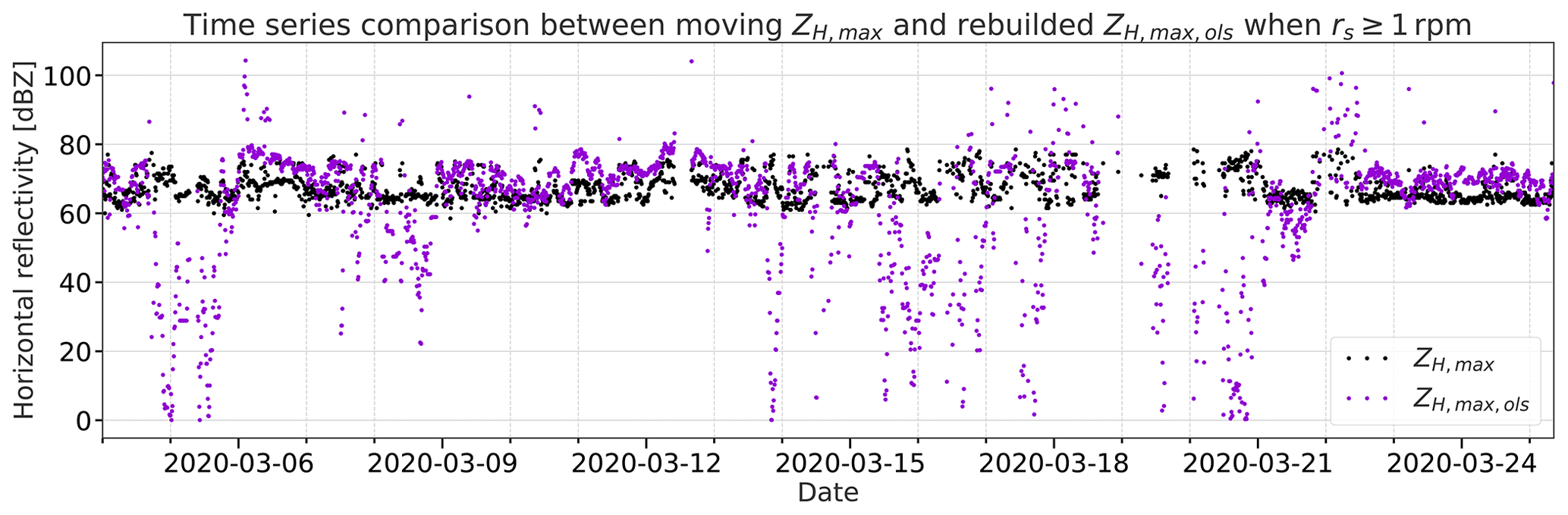
Figure 16Time series scatterplots of the 10 min moving maximum of ZH,max (black) and the corresponding OLS-model-based rebuilt maximum of the horizontal reflectivity (violet) when the rotor speed rs≥1 rpm. For the input of the model estimation, only the WT blade pitch angle θ and nacelle orientation Ψ are used.
The interaction between wind turbines and radar systems is complex in nature due to a large set of parameters affecting the scattering behavior of the turbine object. In this context, MeteoSwiss was in charge of organizing two measurement campaigns, lasting 23 d (2019) and 22 d (2020) each, with a mobile X-band weather radar (METEOR 50DX) in the proximity of the city of Schaffhausen (Switzerland). The area of a small wind park consisting of three large wind turbines was the target area for the radar measurements. The radar was located at a distance between 7.7 and 8.6 km away from the individual wind turbines. There was fairly good visibility towards the three wind turbines. The measurements taken during March 2019 were close to a receiver saturation, while during March 2020 and the fixed-pointing radar observations with the highest returns reaching 78.5 dBZ, a saturation was more likely to happen. Indeed, the observed discrepancy between the correlations of ZH,min and ZH,max with the blade pitch angle θ, for which ZH,min is much more downhill-correlated than ZH,max is uphill-correlated, could be attributed to a receiver saturation issue. So to say, the receiver was not able to capture the highest intrinsic returns from the wind turbine anymore.
At the distance of the wind turbines, the beam size was large enough (∼200 m) to entirely include the complex obstacle within the beam shape. Measurement data have been collected with a scanning sequence composed of slowly moving PPI and RHI scans, with a repetition time of 45 min in March 2019 and with a fixed-pointing antenna observation in March 2020. Although the radar data included polarimetric moments and power spectra, the focus of this paper was the statistical analyses of horizontal reflectivity ZH and radar cross-section (RCS) of large wind turbines for a weather radar operated within the X-band. The maximum returns describe a general worst-case scenario, which is of interest, for example, to the mostly civilian aviation safety sector when measurements from K- or X-band SMRs (surface movement radars) or PARs (precision approach radars) are validated. For the military aviation sector it would also concern radar systems for guidance and surveillance, both for ground-based and airborne systems.
From a comparison point of view, it is worth looking at computational results from Angulo et al. (2015). They also report RCS values on the order of 40 dBsm, with extremely narrow peaks up to 45 to 55 dBsm, for angles of incidence of about 2.5∘. For other angles of incidence large decreases between 15 and 30 dB resulted. Those simulated values do not excessively deviate from our retrieved results. According to those simulations, peak RCSs occur at extremely precise angles of incidence, and the worst-case situations actually can be observed at slightly negative incidence angles (Angulo et al., 2015), a setup that could not be realized with the presented measurement campaigns. In those conditions, for wind turbines of similar size with respect to the ones shown in this report, RCS values can rapidly increase to more than 60 dBsm. For future campaigns it may thus be interesting to perform measurements at a site that allows the observation of wind turbines at negative incidence angles. By using the high temporal continuous radar staring mode, observations up to 44.1 dBsm were reached in case of the closest wind turbine (WT1), with the best visibility from the radar location.
The pattern of the secondary returns depends on the full characteristics of the antenna pattern in all the possible planes, but it is relevant to mention that secondary (or tertiary peaks) have been measured with intensities 20–30 dB lower than the median returns during the measurement campaign in 2019.
Although the derivation of wind turbine RCS is possible by using CEM (commercial computational electromagnetic) tools as proven by Danoon and Brown (2013), the computational requirements are huge, and accounting for the incidence angle, radar range, the rotation of the blades and the yaw angle is difficult and requires very large lookup tables. Thus dedicated measurement campaigns with, for example, mobile radars offer another approach to assess wind turbine reflectivity and RCS in a broad range of real environmental scenarios. Bredemeyer et al. (2019) used a UAS (unmanned aerial system) as a passive bistatic radar (PBR) at nacelle altitude for reflectivity measurements of a wind turbine in the C-band (5.64 GHz). From short distances below 300 m they got RCS differences of more than 30 dB between WT rotor planes perpendicular and parallel to the PBR.
In our study, enhancements of the median ZH could be also related to the WT nacelle orientation, with the highest values being observed when the wind turbine is facing away with respect to the radar location. Interestingly, the 99th percentile of ZH also showed enhancements towards 80–90 and 260–270∘ (sideways-facing towards radar). The reason could not be quantitatively deduced. A combination of an increase in the effective nacelle area (elongated shape) and change in the blade surface due to yawing is a potential source.
A short summary of the key results from the correlation and OLS analyses between the WT and ZH data sets at the 10 min time resolution is given below:
-
The maximum returns increase as the blade pitch angle θ increases, and this is especially true when the wind turbine rotors rotate slowly (sailing or aero-breaking).
-
High variability in ZH,min is observed and a bit less for ZH,max when the blade pitch is at 70∘ or 90∘ (rs<1 rpm).
-
Positive correlation of ZH,max and negative correlation of ZH,min resulted, when the turbine was in normal (power production) operation mode (rs≥1 rpm).
-
For high wind speeds accompanied by aero-breaking pitch angles, we find a highly reduced ZH,max variability compared to sailing WT modes in low wind speeds. Additionally, a moderately positive correlation (ZH,max vs. ) is present for rs below 1 rpm, which could be related to the aero-elastic bending of the blades.
-
By only taking into account the blade pitch angle θ and normalized relative WT orientation parameter Ψ=|sin (α)|, where α corresponds to the relative orientation, an ordinary least square (OLS) model fit shows that more than 90 % of the ZH,max variance can be explained.
Our results can be helpful for wind turbine interference mitigation measures in radar systems in the future. The present detailed description and analysis are based on the first meteorological quantity measured by weather radar in the history of radar meteorology: the so-called radar reflectivity expressed in dBZ. We plan to complement the present work with spectral (mean radial velocity and spectrum width) and polarimetric signatures (co-polar correlation coefficient, differential phase shift, differential reflectivity) of the wind turbines. The next step consists of a stratification of the spectral and polarimetric signatures upon a given rotor speed threshold. Indeed, in the case of not-moving rotors, the WT spectral signatures are similar to those of a tall metallic tower (Gabella, 2018): very large and very stable co-polar correlation coefficient; small dispersion of the differential phase shift; stable and slowly varying horizontal, vertical and differential reflectivities; null spectral signature. An example of not-varying horizontal reflectivity can be seen in Fig. 8a on 19 March. In contrast, in the case of moving rotors, the degree of complexity and interpretation difficulty is similar to what is shown in the present paper, which focuses only on horizontally polarized radar reflectivity.
Pyrad, a real-time data processing framework developed by MeteoSwiss, is available via GitHub under https://github.com/MeteoSwiss/pyrad.git (Figueras i Ventura et al., 2020a) or as a conda-forge package pyrad_mch.
ML prepared the manuscript, did the main data analyses and was involved in setting up the field campaigns. JFiV was in charge of the required software development within Pyrad and helped with the data interpretation. ZS had a leading role in the process of finding the best observation site for the radar system and the setup. MG scientifically advised the team in all aspects of the field campaigns and radar meteorology. With the help of RP, it was possible to get the turbine data from the wind park operator. Further, he advised the team together with MFB on all kinds of wind turbine aspects. JG was, at the time of the measurements, the team lead. He set up the radar and scanning strategies and was involved in the scientific interpretation of the data.
The authors declare that they have no conflict of interest.
The presented work was done in the framework of the project RadarV, a collaboration of MeteoSwiss and armasuisse. Further, we would like to thank Hegauwind GmbH & Co. KG Verenafohren, which kindly provided the operational data of the wind turbines.
This paper was edited by Gianfranco Vulpiani and reviewed by Jochen Bredemeyer and one anonymous referee.
Angulo, I., de la Vega, D., Cascon, I., Canizo, J., Wu, Y., Guerra, D., and Angueira, P.: Impact analysis of wind farms on telecommunication services, Renewable and Sustainable Energy Reviews, 32, 84–99, https://doi.org/10.1016/j.rser.2013.12.055, 2014. a
Angulo, I., Grande, O., Jenn, D., Guerra, D., and de la Vega, D.: Estimating reflectivity values from wind turbines for analyzing the potential impact on weather radar services, Atmos. Meas. Tech., 8, 2183–2193, https://doi.org/10.5194/amt-8-2183-2015, 2015. a, b, c
Battan, L. J.: Radar observation of the atmosphere, University of Chicago press, Chicago, USA, 324 pp., https://doi.org/10.1002/qj.49709942229, 1973. a
Bredemeyer, J., Schubert, K., Werner, J., Schrader, T., and Mihalachi, M.: Comparison of principles for measuring the reflectivity values from wind turbines, in: 2019 20th International Radar Symposium (IRS), pp. 1–10, https://doi.org/10.23919/IRS.2019.8768171, 2019. a
Bringi, V. N. and Chandrasekar, V.: Polarimetric Doppler Weather Radar: Principles and Applications, Cambridge University Press, Cambridge, UK, 636 pp., https://doi.org/10.1017/CBO9780511541094, 2001. a
Cuadra, L., Ocampo-Estrella, I., Alexandre, E., and Salcedo-Sanz, S.: A study on the impact of easements in the deployment of wind farms near airport facilities, Renew. Energ., 135, 566–588, https://doi.org/10.1016/j.renene.2018.12.038, 2019. a, b
Danoon, L. R. and Brown, A. K.: Modeling Methodology for Computing the Radar Cross Section and Doppler Signature of Wind Farms, IEEE Transactions on Antennas and Propagation, 61, 5166–5174, https://doi.org/10.1109/TAP.2013.2272454, 2013. a
de la Vega, D., Jenn, D., Angulo, I., and Guerra, D.: Simplified characterization of Radar Cross Section of wind turbines in the air surveillance radars band, in: 2016 10th European Conference on Antennas and Propagation (EuCAP), Curran Associates, Inc, Red Hook, NY, USA, pp. 1–5, ISBN 978-88-907018-6-3, 2016. a, b
Fabry, F.: Radar Meteorology: Principles and Practice, Cambridge University Press, Cambridge, UK, 256 pp., https://doi.org/10.1017/CBO9781107707405, 2015. a
Figueras i Ventura, J., Lainer, M., Schauwecker, Z., Grazioli, J., and Germann, U.: Pyrad: a Real-Time Weather Radar Data Processing Framework Based on Py-ART, J. Open Res. Softw., 8, 28, https://doi.org/10.5334/jors.330, 2020a (code available at: https://github.com/MeteoSwiss/pyrad.git, last access: 2 May 2021). a, b, c
Figueras i Ventura, J., Schauwecker, Z., Lainer, M., and Grazioli, J.: On the Effect of Radome Characteristics on Polarimetric Moments and Sun Measurements of a Weather Radar, IEEE Geosci. Remote Sens., 18, 642–646, 1–5, https://doi.org/10.1109/LGRS.2020.2981993, 2020b. a
Gabella, M.: On the Use of Bright Scatterers for Monitoring Doppler, Dual-Polarization Weather Radars, Remote Sens., 10, 1007, https://doi.org/10.3390/rs10071007, 2018. a
Gabella, M. and Perona, G.: Simulation of the Orographic Influence on Weather Radar Using a Geometric–Optics Approach, J. Atmos. Ocean. Tech., 15, 1485–1494, https://doi.org/10.1175/1520-0426(1998)015<1485:SOTOIO>2.0.CO;2, 1998. a
Gabella, M., Notarpietro, R., Turso, S., and Perona, G.: Simulated and measured X‐band radar reflectivity of land in mountainous terrain using a fan‐beam antenna, Int. J. Remote Sens., 29, 2869–2878, https://doi.org/10.1080/01431160701596149, 2008. a
Gallardo-Hernando, B., Muñoz-Ferreras, J. M., Pérez-Martínez, F., and Aguado-Encabo, F.: Wind turbine clutter observations and theoretical validation for meteorological radar applications, IET Radar, Sonar & Navigation, 5, 111–117, https://doi.org/10.1049/iet-rsn.2009.0296, 2011. a
Gipe, P.: Wind Power: Renewable Energy for Home, Farm and Business, 2nd edn., Chelsea Green Publishing Co, Vermont, USA, ISBN-13 978-1931498142, 512 pp., 2004. a
He, W., Ma, Y., Shi, Y., Wang, X., Zhang, S., and Wu, R.: Analysis of the wind turbine RCS and micro-Doppler feature based on FEKO, in: 2015 Integrated Communication, Navigation and Surveillance Conference (ICNS), pp. U3-1–U3-9, https://doi.org/10.1109/ICNSURV.2015.7121265, 2015. a
Helmus, J. J. and Collis, S. M.: The Python ARM Radar Toolkit (Py-ART), a library for working with weather radar data in the Python programming language, J. Open Res. Softw., 4, e25, https://doi.org/10.5334/jors.119, 2016. a
Hood, K., Torres, S., and Palmer, R.: Automatic Detection of Wind Turbine Clutter for Weather Radars, J. Atmos. Ocean. Tech., 27, 1868–1880, https://doi.org/10.1175/2010JTECHA1437.1, 2010. a
Kent, B. M., Hil, K. C., Buterbaugh, A., Zelinski, G., Hawley, R., Cravens, L., Tri-Van, Vogel, C., and Coveyou, T.: Dynamic Radar Cross Section and Radar Doppler Measurements of Commercial General Electric Windmill Power Turbines Part 1: Predicted and Measured Radar Signatures, IEEE Antennas and Propagation Magazine, 50, 211–219, https://doi.org/10.1109/MAP.2008.4562424, 2008. a
Knott, E. F., Schaeffer, J. F., and Tulley, M. T.: Radar cross section, SciTech Publishing, Raleigh, NC, USA, ISBN 9781891121258, 611 pp., 2004. a
Komusanac, I., Brindley, G., and Fraile, D.: Wind Energy in Europe in 2019, techreport, WindEurope, Brussels, Belgium, 2020. a
Kong, F., Zhang, Y., Palmer, R., and Bai, Y.: Wind Turbine radar signature characterization by laboratory measurements, in: 2011 IEEE RadarCon (RADAR), pp. 162–166, https://doi.org/10.1109/RADAR.2011.5960520, 2011. a
Lepetit, T., Simon, J., Petex, J., Cheraly, A., and Marcellin, J.: Radar cross-section of a wind turbine: application to weather radars, in: 2019 13th European Conference on Antennas and Propagation (EuCAP), pp. 1–3, 2019. a
Lute, C. and Wieserman, W.: ASR-11 radar performance assessment over a wind turbine farm, in: 2011 IEEE RadarCon (RADAR), pp. 226–230, 2011. a
Muñoz-Ferreras, J., Peng, Z., Tang, Y., Gómez-García, R., Liang, D., and Li, C.: Short-Range Doppler-Radar Signatures from Industrial Wind Turbines: Theory, Simulations, and Measurements, IEEE Transactions on Instrumentation and Measurement, 65, 2108–2119, https://doi.org/10.1109/TIM.2016.2573058, 2016. a
Neely III, R. R., Bennett, L., Blyth, A., Collier, C., Dufton, D., Groves, J., Walker, D., Walden, C., Bradford, J., Brooks, B., Addison, F. I., Nicol, J., and Pickering, B.: The NCAS mobile dual-polarisation Doppler X-band weather radar (NXPol), Atmos. Meas. Tech., 11, 6481–6494, https://doi.org/10.5194/amt-11-6481-2018, 2018. a
Nghiem, A., Pineda, I., and Tardieu, P.: Wind energy in Europe: Scenarios for 2030, Technical report available from Wind EUROPE, Brussels, Belgium, p. 32, 2017. a
Norin, L.: A quantitative analysis of the impact of wind turbines on operational Doppler weather radar data, Atmos. Meas. Tech., 8, 593–609, https://doi.org/10.5194/amt-8-593-2015, 2015. a
Norin, L.: Wind turbine impact on operational weather radar I/Q data: characterisation and filtering, Atmos. Meas. Tech., 10, 1739–1753, https://doi.org/10.5194/amt-10-1739-2017, 2017. a
Probert-Jones, J. R.: The radar equation in meteorology, Q. J. Roy. Meteorol. Soc., 88, 485–495, https://doi.org/10.1002/qj.49708837810, 1962. a
Ryzhkov, A. V. and Zrnic, D. S.: Radar Polarimetry for Weather Observations, Springer, Cham, Switzerland, 486 pp., https://doi.org/10.1007/978-3-030-05093-1, ISBN 978-3-030-05093-1, 2019. a
Seabold, S. and Perktold, J.: Statsmodels: Econometric and statistical modeling with python, in: Proceedings of the 9th Python in Science Conference, vol. 57, p. 61, Austin, TX, 2010. a
Skolnik, M. I.: Radar handbook second edition, McGraw-Hill Professional, New York, NY, USA, ISBN 978-0070579132, 1200 pp., 1990. a
Weisshaar, T. A.: Aeroelastic Tailoring of Forward Swept Composite Wings, Jo. Aircraft, 18, 669–676, https://doi.org/10.2514/3.57542, 1981. a
Zhang, S., Franek, O., Byskov, C., and Pedersen, G. F.: Antenna Gain Impact on UWB Wind Turbine Blade Deflection Sensing, IEEE Access, 6, 20497–20505, https://doi.org/10.1109/ACCESS.2018.2819880, 2018. a