Machine learning calibration of low-cost NO₂ and PM₁₀ sensors: non-linear algorithms and their impact on site transferability

Low-cost air pollution sensors often fail to attain sufficient performance compared with state-of-the-art measurement stations, and they typically require expensive laboratory-based calibration procedures. A repeatedly proposed strategy to overcome these limitations is calibration through co-location with public measurement stations. Here we test the idea of using machine learning algorithms for such calibration tasks using hourly-averaged co-location data for nitrogen dioxide (NO₂) and particulate matter of particle sizes smaller than 10 µm (PM₁₀) at three different locations in the urban area of London, UK. We compare the performance of ridge regression, a linear statistical learning algorithm, to two non-linear algorithms in the form of random forest regression (RFR) and Gaussian process regression (GPR). We further benchmark the performance of all three machine learning methods relative to the more common multiple linear regression (MLR). We obtain very good out-of-sample R² scores (coefficient of determination) >0.7, frequently exceeding 0.8, for the machine learning calibrated low-cost sensors. In contrast, the performance of MLR is more dependent on random variations in the sensor hardware and co-located signals, and it is also more sensitive to the length of the co-location period. We find that, subject to certain conditions, GPR is typically the best-performing method in our calibration setting, followed by ridge regression and RFR. We also highlight several key limitations of the machine learning methods, which will be crucial to consider in any co-location calibration. In particular, all methods are fundamentally limited in how well they can reproduce pollution levels that lie outside those encountered at training stage. We find, however, that the linear ridge regression outperforms the non-linear methods in extrapolation settings. GPR can allow for a small degree of extrapolation, whereas RFR can only predict values within the training range. This algorithm-dependent ability to extrapolate is one of the key limiting factors when the calibrated sensors are deployed away from the co-location site itself. Consequently, we find that ridge regression is often performing as good as or even better than GPR after sensor relocation. Our results highlight the potential of co-location approaches paired with machine learning calibration techniques to reduce costs of air pollution measurements, subject to careful consideration of the co-location training conditions, the choice of calibration variables and the features of the calibration algorithm.

1 Introduction

Air pollutants such as nitrogen dioxide (NO₂) and particulate matter (PM) have harmful impacts on human health, the ecosystem and public infrastructure (European Environment Agency, 2019). Moving towards reliable and high-density air pollution measurements is consequently of prime importance. The development of new low-cost sensors, hand in hand with novel sensor calibration methods, has been at the forefront of current research efforts in this discipline (e.g. Mead et al., 2013; Moltchanov et al., 2015; Lewis et al., 2018; Zimmerman et al., 2018; Sadighi et al., 2018; Tanzer et al., 2019; Eilenberg et al., 2020; Sayahi et al., 2020). Here we present insights from a case study using low-cost air pollution sensors for measurements at three separate locations in the urban area of London, UK. Our focus is on testing the advantages and disadvantages of machine learning calibration techniques for low-cost NO₂ and PM₁₀ sensors. The principal idea is to calibrate the sensors through co-location with established high-performance air pollution measurement stations (Fig. 1). Such calibration techniques, if successful, could complement more expensive laboratory-based calibration approaches, thereby further reducing the costs of the overall measurement process (e.g. Spinelle et al., 2015; Zimmerman et al., 2018; Munir et al., 2019). For the sensor calibration, we compare three machine learning regression techniques in the form of ridge regression, random forest regression (RFR) and Gaussian process regression (GPR), and we contrast the results to those obtained with standard multiple linear regression (MLR). RFR has been studied in the context of NO₂ co-location calibrations before, with very promising results (Zimmerman et al., 2018). Equally for NO₂ (but not for PM₁₀) different linear versions of GPR have been tested by De Vito et al. (2018) and Malings et al. (2019). To the best of our knowledge, we are the first to test ridge regression both for NO₂ and PM₁₀ and GPR for PM₁₀. Finally, we also investigate well-known issues concerning site transferability (Masson et al., 2015; Fang and Bate, 2017; Hagan et al., 2018; Malings et al., 2019), i.e. if a calibration through co-location at one location gives rise to reliable measurements at a different location.

A key motivation for our study is the potential of low-cost sensors (costs of the order of GBP 10 to GBP 100) to transform the level of availability of air pollution measurements. Installation costs of state-of-the-art measurement stations typically range between GBP 10 000 and GBP 100 000 per site, and those already high costs are further exacerbated through subsequent maintenance and calibration requirements (Mead et al., 2013; Lewis et al., 2016; Castell et al., 2017). Lower measurement costs would allow for the deployment of denser air pollution sensor networks and for portable devices possibly even at the exposure level of individuals (Mead et al., 2013). A central complication is the sensitivity of sensors to environmental conditions such as temperature and relative humidity (Masson et al., 2015; Spinelle et al., 2015; Jiao et al., 2016; Lewis et al., 2016; Spinelle et al., 2017; Castell et al., 2017) or to cross-sensitivities with other gases (e.g. nitrogen oxide), which can significantly impede their measurement performance (Mead et al., 2013; Popoola et al., 2016; Rai and Kumar, 2018; Lewis et al., 2018; Liu et al., 2019). Low-cost sensors thus require, in the same way as many other measurement devices, sophisticated calibration techniques. Machine learning regressions have seen increased use in this context due to their ability to calibrate for many simultaneous, non-linear dependencies. These dependencies, in turn, can for example be assessed in relatively expensive laboratory settings. However, even laboratory calibrations do not always perform well in the field (Castell et al., 2017; Zimmerman et al., 2018). Here, we instead evaluate the performance of low-cost sensor calibrations based on co-location measurements with established reference stations (e.g. Masson et al., 2015; Spinelle et al., 2015; Esposito et al., 2016; Lewis et al., 2016; Cross et al., 2017; Hagan et al., 2018; Casey and Hannigan, 2018; Casey et al., 2019; De Vito et al., 2018, 2019; Zimmerman et al., 2018; Casey et al., 2019; Munir et al., 2019; Malings et al., 2019, 2020). If sufficiently successful, these methods could help to substantially reduce the overall costs and simplify the process of calibrating low-cost sensors.

Another challenge in relation to co-location calibration procedures is “site transferability”. This term refers to the measurement performance implications of moving a calibrated device from one location (where the calibration was conducted) to another location. Some significant performance losses after site transfers have been reported (e.g. Fang and Bate, 2017; Casey and Hannigan, 2018; Hagler et al., 2018; Vikram et al., 2019), with reasons typically not being straightforward to assign. A key driver might be that often devices are calibrated in an environment not representative of situations found in later measurement locations. As we discuss in greater detail below, for machine-learning-based calibrations this behaviour can, to a degree, be fairly intuitively explained by the fact that they do not tend to perform well when extrapolating beyond their training domain. As we will show, this issue can easily occur in situations where already calibrated sensors have to measure pollution levels well beyond the range of values encountered in their training environment.

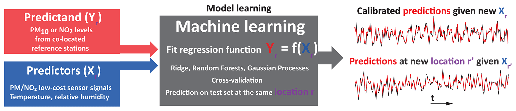
Figure 1 Sketch of the co-location calibration methodology. We co-locate several low-cost sensors for PM (for various particle sizes) and NO₂ with higher-cost reference measurement stations for PM₁₀ and NO₂. The low-cost sensors also measure relative humidity and temperature as key environmental variables that can interfere with the sensor signals, and for NO₂ calibrations, we further include nitrogen oxide (NO) sensors. We formulate the calibration task as a regression problem in which the low-cost sensor signals and the environmental variables are the predictors (X_r) and the reference station signal the predictand (Y_r), both measured at the same location r. The time resolution is set to hourly averages to match publicly available reference data. We train separate calibration functions for each NO₂ and PM₁₀ sensor, and we compare three different machine learning algorithms (ridge, random forest and Gaussian process regressions) with multiple linear regression in terms of their respective calibration performances. The performance is evaluated on out-of-sample test data, i.e. on data not used during training. Once trained and cross-validated, we use these calibration functions to predict PM₁₀ and NO₂ concentrations given new low-cost measurements X, either measured at the same location r or at a new location r^′. The latter location is to test the feasibility and impacts of changing measurement sites post-calibration. The time series (right) are for illustration purposes only.

We highlight that, in particular concerning the performance of low-cost PM₁₀ sensors, a huge gap in the scientific literature has been identified regarding issues related to co-location calibrations (Rai and Kumar, 2018). We therefore expect that our study will provide novel insights into the effects of different calibration techniques on sensor performances, and a data sample that other measurement studies from academia and industry can compare their results against. We will mainly use the R² score (coefficient of determination) and root mean squared error (RMSE) as metrics to evaluate our calibration results, which are widely used and should thus facilitate intercomparisons. To provide a reference for calibration results perceived as “good” for PM₁₀, we point towards a sensor comparison by Rai and Kumar (2018), who found that low-cost sensors generally displayed moderate to excellent linearity (R²>0.5) across various calibration settings. The sensors typically perform particularly well (R²>0.8) when tested in idealized laboratory conditions. However, their performance is generally lower in field deployments (see also Lewis et al., 2018). For PM₁₀, this performance deterioration was, inter alia, attributed to changing conditions of particle composition, particle sizes and environmental factors such as humidity and temperature, which are thus important factors to account for in our calibrations.

The structure of our paper is as follows. In Sect. 2, we introduce the low-cost sensor hardware used, the reference measurement sources, the three measurement site characteristics and measurement periods, the four calibration regression methods, and the calibration settings (e.g. measured signals used) for NO₂ and PM₁₀. In Sect. 3, we first introduce multi-sensor calibration results for NO₂ at a single site, depending on the sensor signals included in the calibrations and the number of training samples used to train the regressions. This is followed by a discussion of single-site PM₁₀ calibration results before we test the feasibility and challenges of site transfers. We discuss our results and draw conclusions in Sect. 4.

2 Methods and data

2.1 Sensor hardware

Depending on the measurement location, we deployed one set or several sets of air pollution sensors, and we refer to each set (provided by London-based AirPublic Ltd) as a multi-sensor “node”. Each of these nodes consists of multiple electrochemical and metal oxide sensors for PM and NO₂, as well as sensors for environmental quantities and other chemical species known for potential interference with their sensor signals (required for calibration). Each node thus allows for simultaneous measurement of multiple air pollutants, but we will focus on individual calibrations for NO₂ and PM₁₀ here, because these species were of particular interest to our own measurement campaigns. We note that other species such as PM_2.5 are also included in the measured set of variables. We will make our low-cost sensor data available (see “Data availability” section), which will allow other users to test similar calibration procedures for other variables of interest (e.g. PM_2.5, ozone). A caveat is that appropriate co-location data from higher-cost reference measurements might not always be available.

For NO₂, we incorporated three different types of sensors in our set-up for which purchasing prices differed by an order of magnitude. One aspect of our study will therefore be to evaluate the performance gained by using the more expensive (but still relatively low-cost) sensor types. Of course, our results will only be validated in the context of our specific calibration method so that more general conclusions have to be drawn with care.

Each multi-sensor node contained the following (i.e. all nodes consist of the same types of individual sensors):

• Two MiCS-2714 NO₂ sensors produced by SGX Sensortech. These are the cheapest measurement devices deployed in our set with market costs of approximately GBP 5 per sensor.

• Two Plantower PMS5003T series PM sensors (PMSs), which measure particles of various size categories including PM₁₀ based on laser scattering using Mie theory. We note that particle composition does play a role in any PM calibration process as, for example, organic materials tend to absorb a higher proportion of incident light as compared to inorganic materials (Rai and Kumar, 2018). Below we therefore effectively make the assumption that we measure and calibrate within composition-wise similar environments. By taking into account various particle size measures in the calibration, we likely do indirectly account for some aspects of composition though, because to a degree, particle sizes might be correlated with particle composition. Each PMS device also contains a temperature and relative humidity sensor, and these variables were also included in our calibrations. The minimum distinguishable particle diameter for the PMS devices is 0.3 µm. The market cost is GBP 20 for one sensor.

• An NO2-A43F four-electrode NO₂ sensor produced by AlphaSense (market cost GBP 45).

• An NO2-B43F four-electrode NO₂ sensor produced by AlphaSense (market cost GBP 45).

• An NO-A4 four-electrode nitric oxide sensor produced by AlphaSense to calibrate against the sometimes significant interference of NO₂ signals with NO (market cost GBP 45).

• An OX-A431 four-electrode oxidizing gas sensor measuring a combined signal from ozone and NO₂ produced by AlphaSense. We used this signal to calibrate against possible interference of electrochemical NO₂ measurements by ozone (market cost GBP 45).

• A separate temperature sensor built into the AlphaSense set. It is needed to monitor the warm-up phase of the sensors.

In normal operation mode, each node provided measurements around every 30 s. These signals were time-averaged to hourly values for calibration against hourly public reference measurements.

2.2 Measurement sites and reference monitors

We conducted measurements at three sites in the Greater London area during distinct multi-week periods (Table 1). Two of the sites are located in the London Borough of Croydon, which we label CR7 and CR9 according to their UK postcodes. The third site is located in the car park of the company AlphaSense in Essex, hereafter referred to as site “CarPark” (Fig. 2a). At CR7, the sensor nodes were located kerbside on a medium busy street with two lanes in either direction. At CR9, the nodes were located on a traffic island in the middle of a very busy road with three lanes in either direction (Fig. 2b). For the two Croydon sites, reference measurements were obtained from co-located, publicly available measurements of London's Air Quality Network (LAQN; https://www.londonair.org.uk, last access: 30 April 2020​​​​​​​). In the two locations in question, the LAQN used chemiluminescence detectors for NO₂ and Thermo Scientific tapered element oscillating microbalance (TEOM) continuous ambient particulate monitors, with the Volatile Correction Model (Green et al., 2009) for PM₁₀ measurements at CR9. For the CarPark site, PM₁₀ measurements were conducted with a Palas Fidas optical particle counter AFL-W07A. These CarPark reference measurements were provided at 15 min intervals. For consistency, these measurements were averaged to hourly values to match the measurement frequency of publicly available data at the other two sites.

Table 1 Overview of the measurement sites and the corresponding maximum co-location periods, which vary for each specific sensor node and co-location site due to practical aspects such as sensor availability and random occurrences of sensor failures. Note that reference measurements for NO₂ and PM₁₀ are only available for two of the three sites each. Sensors that were co-located for at least 820 active measurement hours are identified by their sensor IDs in the last column. Further note that the only sensor used to measure at multiple sites is sensor 19, which is therefore used to test the feasibility of site transfers.

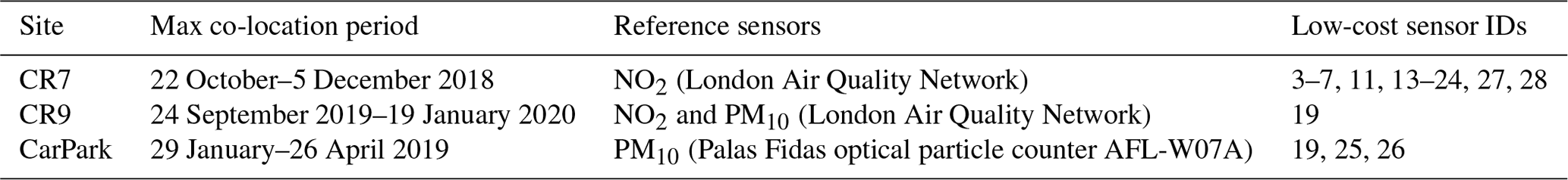
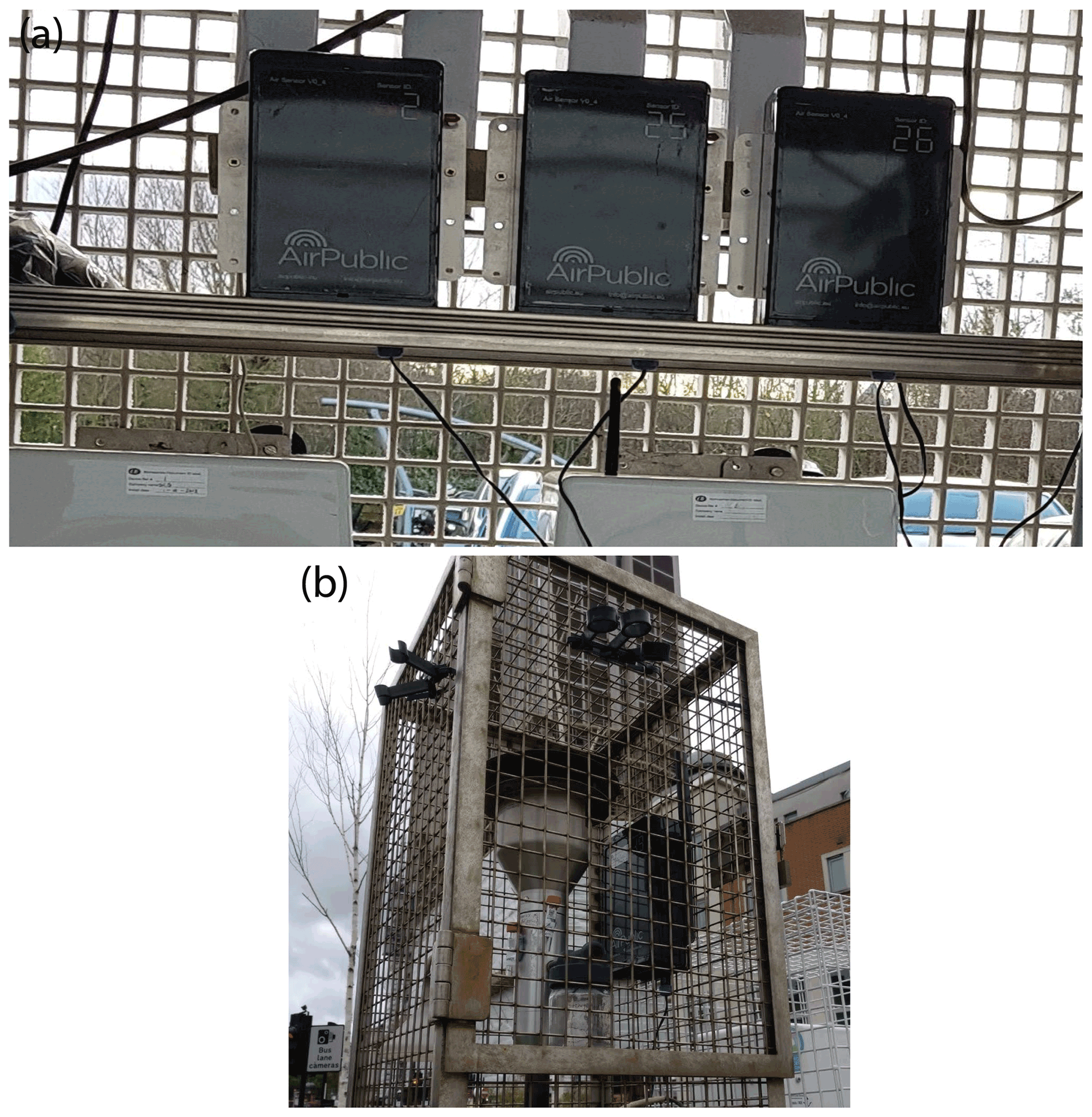
Figure 2 Examples of the co-location set-up of the AirPublic low-cost sensor nodes with reference measurement stations at sites (a) CarPark and (b) CR9.

2.3 Co-location set-up and calibration variables

In total, we co-located up to 30 nodes, labelled by identifiers (IDs) 1 to 30. For our NO₂ measurements, we considered the following 15 sensor signals per node to be important for the calibration process: the NO sensor (plus its baseline signal to remove noise), the NO₂ + O₃ sensor (plus baseline), the two intermediate cost NO₂ sensors (NO2-A43F, NO2-B43F) plus their respective baselines, the two cheaper MiCS sensors, three different temperature sensors, and two relative humidity sensors. All 15 signals can be used for calibration against the reference measurements obtained with the co-located higher-cost measurement devices. We discuss the relative importance of the different signals, e.g. the relative importance of the different NO₂ sensors or the influence of temperature and humidity in Sect. 3. For the PM₁₀ calibrations, we used two devices of the same type of low-cost PM sensor, resulting in 2×10 different particle measures used in the PM₁₀ calibrations. In addition, we included the respective sensor signals for temperature and relative humidity, providing us with in total 24 calibration signals for PM₁₀.

2.4 Calibration algorithms

We evaluate four regression calibration strategies for low-cost NO₂ and PM₁₀ devices, by means of co-location of the devices with the aforementioned air quality measurement reference stations. The four different regression methods – which are multiple linear regression (MLR), ridge regression, random forest regression (RFR) and Gaussian process regression (GPR) – are introduced in detail in the following subsections. As we will show in Sect. 3, the relative skill of the calibration methods depends on the chemical species to be measured, sample size available for calibration, and certain user preferences. We will additionally consider the issue of site transferability for sensor node 19, including its dependence on the calibration algorithm used. We note that we do not include the manufacturer calibration of the low-cost sensors in our comparison here mainly because we found that this method, which is a simple linear regression based on certain laboratory measurement relationships, provided us with negative R² scores when compared with reference sensors in the field. This result is in line with other studies that reported differences between sensor performances in the field and under laboratory calibrations (see e.g. Mead et al., 2013; Lewis et al., 2018; Rai and Kumar, 2018).

2.4.1 Ridge and multiple linear regression

Ridge regression is a linear least squares regression augmented by L₂ regularization to address the bias-variance trade-off (Hoerl and Kennard, 1970; James et al., 2013; Nowack et al., 2018, 2019). Using statistical cross-validation, the regression fit is optimized by minimizing the cost function

$$\begin{array}{}\text{(1)}& J_{\text{Ridge}}=\sum _{t=\mathrm{1}}^n{\left(y_t-\sum _{j=\mathrm{1}}^p{c}_j{x}_{j,t}\right)}^{\mathrm{2}}+\mathit{\alpha }\sum _{j=\mathrm{1}}^p{c}_j^{\mathrm{2}}\end{array}$$

over n hourly reference measurements of pollutant y (i.e. NO₂, PM₁₀); x_j,t represents p non-calibrated measurement signals from the low-cost sensors, representing signals for the pollutant itself as well as signals recorded for environmental variables (temperature, humidity) and other chemical species that might cause interference with the signal in question. The cost function (Eq. 1) determines the optimization goal. Its first term is the ordinary least squares regression error, and the second term puts a penalty on too large regression coefficients and thus avoids overfitting in high-dimensional settings. Smaller (larger) values of the regularization coefficient α put weaker (stronger) constraints on the size of the coefficients, thereby favouring overfitting (high bias). We find the value for α through fivefold cross-validation; i.e. each data set is split into five ordered time slices and α optimized by fitting regressions for large ranges of α values on four of the slices at a time, and then the best α is found by evaluating the out-of-sample prediction error on each corresponding remaining slice using the R² score. Each slice is used once for the evaluation step. Before the training procedure, all signals are scaled to unit variance and zero mean so as to ensure that all signals are weighted equally in the regression optimization, which we explain in more detail at the end of this section. Through the constraint on the regression slopes, ridge regression can handle settings with many predictors, here calibration variables, even in the context of strong collinearity in those predictors (Dormann et al., 2013; Nowack et al., 2018, 2019). The resulting linear regression function f_Ridge,

$$\begin{array}{}\text{(2)}& \widehat{y}\left(t\right)=f_{\text{Ridge}}=c_{\mathrm{0}}+\sum _{j=\mathrm{1}}^p{c}_j{x}_j\left(t\right),\end{array}$$

provides estimates for pollutant mixing ratios $\widehat{y}$ at any time t, i.e. a calibrated low-cost sensor signal, based on new sensor readings x_j(t). f_Ridge represents a calibration function because it is not just based on a regression of the pollutant signal itself against the reference but also on multiple simultaneous predictors, including those representing known interfering factors.

Multiple linear regression (MLR) is the simple non-regularized case of ridge regression, i.e. where α is set to nil. MLR is therefore a good benchmark to evaluate the importance of regularization and, when compared to RFR and GPR below, of non-linearity in the relationships. As MLR does not regularize its coefficients, it is expected to increasingly lose performance in settings with many (non-linear) calibration relationships. This loss of MLR performance in high-dimensional regression spaces is related to the “curse of dimensionality” in machine learning, which expresses the observation that one requires an exponentially increasing number of samples to constrain the regression coefficients as the number of predictors is increased linearly (Bishop, 2006). We will illustrate this phenomenon for the case of our NO₂ sensor calibrations below.

Finally, we note that for ridge regression, as also for GPR described below, the predictors x_j must be normalized to a common range. For ridge, this is straightforward to understand as the regression coefficients, once the predictors are normalized, provide direct measures of the importance of each predictor for the overall pollutant signal. If not normalized, the coefficients will additionally weight the relative magnitude of predictor signals, which can differ by orders of magnitude (e.g. temperature at around 273 K but a measurement signal for a trace gas of the order of 0.5 amplifier units). As a result, the predictors would be penalized differently through the same α in Eq. (1), which could mean that certain predictors are effectively not considered in the regressions. Here, we normalize all predictors in all regressions to zero mean and unit standard deviation according to the samples included in each training data set.

2.4.2 Random forest regression

Random forest regression (RFR) is one of the most widely used non-linear machine learning algorithms (Breiman and Friedman, 1997; Breiman, 2001), and it has already found applications in air pollution sensor calibration as well as in other aspects of atmospheric chemistry (Keller and Evans, 2019; Nowack et al., 2018, 2019; Sherwen et al., 2019; Zimmerman et al., 2018; Malings et al., 2019). It follows the idea of ensemble learning where multiple machine learning models together make more reliable predictions than the individual models. Each RFR object consists of a collection (i.e. ensemble) of graphical tree models, which split training data by learning decision rules (Fig. 3). Each of these decision trees consists of a sequence of nodes, which branch into multiple tree levels until the end of the tree (the “leaf” level) is reached. Each leaf node contains at least one or several samples from the training data. The average of these samples is the prediction of each tree for any measurement of predictors x defining a new traversion of the tree to the given leaf node. In contrast to ridge regression, there is more than one tunable hyperparameter to address overfitting. One of these hyperparameters is the maximum tree depth, i.e. the maximal number of levels within each tree, as deeper trees allow for a more detailed grouping of samples. Similarly, one can set the minimum number of samples in any leaf node. Once this minimum number is reached, the node is not further split into children nodes. Both smaller tree depth and a greater number of minimum samples in leaf nodes mitigate overfitting to the training data. Other important settings are the optimization function used to define the decision rules and, for example, the number of estimators included in an ensemble, i.e. the number of trees in the forest.

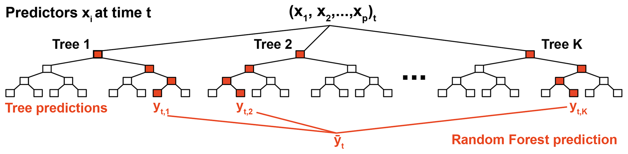
Figure 3 Sketch of a random forest regressor. Each random forest consists of an ensemble of K trees. For visualization purposes, the trees shown here have only four levels of equal depth, but more complex structures can be learnt. The lowest level contains the leaf nodes. Note that in real examples, branches can have different depths; i.e. the leaf nodes can occur at different levels of the tree hierarchy; see, for example, Fig. 2 in Zimmerman et al. (2018). Once the decision rules for each node and tree are learnt from training data, each tree can be presented with new sensor readings x at a time t to predict pollutant concentration y_t. The decision rules depend, inter alia, on the tree structure and random sampling through bootstrapping, which we optimize through fivefold cross-validation. Based on the values x_i, each set of predictors follows routes through the trees. The training samples collected in the corresponding leaf node define the tree-specific prediction for y. By averaging K tree-wise predictions, we combat tree-specific overfitting and finally obtain a more regularized random forest prediction ${\stackrel{\mathrm{‾}}{y}}_t$.

The RFR training process tunes the parameter thresholds for each binary decision tree node. By introducing randomness, e.g. by selecting a subset of samples from the training data set (bootstrapping), each tree provides a somewhat different data representation. This random element is used to obtain a better, averaged prediction over all trees in the ensemble, which is less prone to overfitting than individual regression trees. We here cross-validated the scikit-learn implementation of RFR (Pedregosa et al., 2011) over problem-specific ranges for the minimum number of samples required to define a split and the minimum number of samples to define a leaf node. The implementation uses an optimized version of the Classification And Regression Tree (CART) algorithm, which constructs binary decision trees using the predictor and threshold that yields the largest information gain for a split at each node. The mean squared error of samples relative to their node prediction (mean) serves as optimization criterion so as to measure the quality of a split for a given possible threshold during training. Here we consider all features when defining any new best split of the data at nodes. By increasing the number of trees in the ensemble, the RFR generalization error converges towards a lower limit. We here set the number of trees in all regression tasks to 200 as a compromise between model convergence and computational complexity (Breiman, 2001).

2.4.3 Gaussian process regression

Gaussian process regression (GPR) is a widely used Bayesian machine learning method to estimate non-linear dependencies (Rasmussen and Williams, 2006; Pedregosa et al., 2011; Lewis et al., 2016; De Vito et al., 2018; Runge et al., 2019; Malings et al., 2019; Nowack et al., 2020; Mansfield et al., 2020). In GPR, the aim is to find a distribution over possible functions that fit the data. We first define a prior distribution of possible functions that is updated according to the data using Bayes' theorem, which provides us with a posterior distribution over possible functions. The prior distribution is a Gaussian process (GP),

$$\begin{array}{}\text{(3)}& Y\sim \text{GP}\left(\mathit{\mu },k(x_i,x_j)\right),\end{array}$$

with mean μ and a covariance function or kernel k, which describes the covariance between any two points x_i and x_j. We here “standard-scale” (i.e. centre) our data so that μ=0, meaning our GP is entirely defined by the covariance function. Being a kernel method, the performance of GPR depends strongly on the kernel (covariance function) design as it determines the shape of the prior and posterior distributions of the Gaussian process and in particular the characteristics of the function we are able to learn from the data. Owing to the time-varying, continuous but also oscillating nature of air pollution sensor signals, we here use a sum kernel of a radial basis function (RBF) kernel, a white noise kernel, a Matérn kernel and a “Dot-Product” kernel. The RBF kernel, also known as squared exponential kernel, is defined as

$$\begin{array}{}\text{(4)}& k(x_i,x_j)=\exp \left({\displaystyle \frac{-d(x_i,x_j{)}^{\mathrm{2}}}{\mathrm{2}{l}^{\mathrm{2}}}}\right).\end{array}$$

It is parameterized by a length scale l>0, and d is the Euclidean distance. The length scale determines the scale of variation in the data, and it is learnt during the Bayesian update; i.e. for a shorter length scale the function is more flexible. However, it also determines the extrapolation scale of the function, meaning that any extrapolation beyond the length scale is probably unreliable. RBF kernels are particularly helpful to model smooth variations in the data. The Matérn kernel is defined by

$$\begin{array}{}\text{(5)}& \begin{array}{rl}k(x_i,x_j)=& {\displaystyle \frac{\mathrm{1}}{\mathrm{\Gamma }\left(\mathit{\nu }\right){\mathrm{2}}^{\mathit{\nu }-\mathrm{1}}}}{\left({\displaystyle \frac{\sqrt{\mathrm{2}\mathit{\nu }}}{l}}d(x_i,x_j)\right)}^{\mathit{\nu }}{K}_{\mathit{\nu }}\\ & \left({\displaystyle \frac{\sqrt{\mathrm{2}\mathit{\nu }}}{l}}d(x_i,x_j)\right),\end{array}\end{array}$$

where K_ν is a modified Bessel function and Γ the gamma function (Pedregosa et al., 2011). We here choose ν=1.5 as the default setting for the kernel, which determines the smoothness of the function. Overall, the Matérn kernel is useful to model less-smooth variations in the data than the RBF kernel. The Dot-Product kernel is parameterized by a hyperparameter ${\mathit{\sigma }}_{\mathrm{0}}^{\mathrm{2}}$,

$$\begin{array}{}\text{(6)}& k(x_i,x_j)={\mathit{\sigma }}_{\mathrm{0}}^{\mathrm{2}}+x_i\cdot x_j,\end{array}$$

and we found that adding this kernel to the sum of kernels improved our results empirically. The white noise kernel simply allows for a noise level on the data as independently and identically normally distributed, specified through a variance parameter. This parameter is similar to (and will interact with) the α noise level described below, which is, however, tested systematically through cross-validation.

The Python scikit-learn implementation of the algorithm used here is based on Algorithm 2.1 of Rasmussen and Williams (2006). We optimized the kernel parameters in the same way as for the other regression methods through fivefold cross-validation, and we subject them to the noise α parameter of the scikit-learn GPR regression packages (Pedregosa et al., 2011). This parameter is not to be confused with the α regularization parameter for ridge regression and takes the role of smoothing the kernel function so as to address overfitting. It represents a value added to the diagonal of the kernel matrix during the fitting process with larger α values corresponding to greater noise level in the measurements of the outputs. However, we note that there is some equivalency with the α parameter in ridge as the method is effectively a form of Tikhonov regularization that is also used in ridge regression (Pedregosa et al., 2011). Both inputs and outputs to the GPR function were standard-scaled to zero mean and unit variance based on the training data. For each GPR optimization, we chose 25 optimizer restarts with different initializations of the kernel parameters, which is necessary to approximate the best possible solution to maximize the log-marginal likelihood of the fit. More background on GPR can be found in Rasmussen and Williams (2006).

2.5 Cross-validation

For all regression models, we performed fivefold cross-validation where the data are first split into training and test sets, keeping samples ordered by time. The training data are afterwards divided into five consecutive subsets (folds) of equal length. If the training data are not divisible by five, with a residual number of samples n, then the first n folds will contain one surplus sample compared to the remaining folds. Each fold is used once as a validation set, while the remaining four folds are used for training. The best set of model hyperparameters or kernel functions is found according to the average generalization error on these validation sets. After the best cross-validated hyperparameters are found, we refit the regression models on the entire training data using these hyperparameter settings (e.g. the α value for which we found the best out-of-sample performance for ridge regression).

3 Results

3.1 NO₂ sensor calibration

The skill of a sensor calibration function is expected to increase with sample size, i.e. the number of measurements used in the calibration process, but will also depend on aspects of the sampling environment. For co-location measurements, there will be time-dependent fluctuations in the value ranges encountered for the predictors (e.g. low-cost sensor signals, humidity, temperature) and predictands (reference NO₂, PM₁₀). The calibration range in turn affects the performance of the calibration function: if faced with values outside its training range, the function effectively has to perform an extrapolation rather than interpolation, i.e. the function is not well constrained outside its training domain. This limitation is particularly critical for non-linear machine learning functions (Hagan et al., 2018; Nowack et al., 2018; Zimmerman et al., 2018). Calibration performance will further vary for each device, even for sensors of the same make, due to unavoidable randomness in the sensor production process (Mead et al., 2013; Castell et al., 2017). To characterize these various influences, we here test the dependence of three machine learning calibration methods, as well as of MLR, on sample size and co-location period for a number of NO₂ sensors.

The NO₂ co-location data at CR7 is ideally suited for this purpose. Twenty-one sensor nodes of the same make were co-located with a LAQN reference during the period October to December 2018 (Table 1). We actually co-located 30 sensor sets at the site, but we excluded any sensors with less than 820 h (samples) after outlier removal from our evaluation. The remaining sensors measure sometimes overlapping but still distinct time periods, because each sensor measurement varied in its precise co-location start and end time and was also subject to sensor-specific periods of malfunction. To detect these malfunctions, and to exclude the corresponding samples, we removed outliers (evidenced by unrealistically large measurement signals) at the original time resolution of our measurements, i.e. <1 min and prior to hourly averaging. To detect outliers for removal, we used the median absolute deviation (MAD) method, also known as “robust Z-Score method”, which identifies outliers for each variable based on their univariate deviation from their training data median. Since the median is a robust statistic to outliers itself, it is a typically a better measure to identify outliers than, for example, a deviation from the mean. Accordingly, we excluded any samples t from the training and test data where the quantity

$$\begin{array}{}\text{(7)}& M_{j,t}=\mathrm{0.6745}{\displaystyle \frac{|x_{j,t}-{\stackrel{\mathrm{̃}}{x}}_j|}{\text{median}\left\{|x_{j,t}-{\stackrel{\mathrm{̃}}{x}}_j|\right\}}}\end{array}$$

takes on values >7 for any of the predictors, where ${\stackrel{\mathrm{̃}}{x}}_j$ is the training data median value of each predictor. To train and cross-validate our calibration models, we took the first 820 h measured by each sensor set and split it into 600 h for training and cross-validation, leaving 220 h to measure the final skill on an out-of-sample test set. We highlight again that the test set will cover different time intervals for different sensors, meaning that further randomness is introduced in how we measure calibration skill. However, the relationships for each of the four calibration methods are learnt from exactly the same data and their predictions are also evaluated on the same data, meaning that their robustness and performance can still be directly compared. To measure calibration skill, we used two standard metrics in the form of the R² score (coefficient of determination), defined by

$$\begin{array}{}\text{(8)}& R^{\mathrm{2}}(y,\widehat{y})=\mathrm{1}-{\displaystyle \frac{{\sum }_{i=\mathrm{1}}^n(y_i-{\widehat{y}}_i{)}^{\mathrm{2}}}{{\sum }_{i=\mathrm{1}}^n(y_i-\stackrel{\mathrm{‾}}{y}{)}^{\mathrm{2}}}},\end{array}$$

and the RMSE between the reference measurements y and our calibrated signals $\widehat{y}$ on the test sets. For particularly poor calibration functions, the R² score can take on infinitely negative values, whereas a value of 1 implies a perfect prediction. An R² score of 0 is equivalent to a function that predicts the correct long-term time average of the data but no fluctuations therein.

As discussed in Sect. 2.1, each of AirPublic's co-location nodes measures 15 signals (the predictors or inputs) that we consider relevant for the NO₂ sensor calibration against the LAQN reference signal for NO₂ (the predictand or output). Each of the 15 inputs will potentially be systematically linearly or non-linearly correlated with the output, which allows us to learn a calibration function from the measurement data. Once we know this function, we should be able to make accurate predictions given new inputs to reproduce the LAQN reference. As we fit two linear and two non-linear algorithms, certain transformations of the inputs can be useful to facilitate the learning process. For example, a relationship between an input and the output might be an exponential dependence in the original time series so that applying a logarithmic transformation could lead to an approximately linear relationship that might be easier to learn for a linear regression function. We therefore compared three set-ups with different sets of predictors:

1. using the 15 input time series as provided (label I₁₅);

2. adding logarithmic transformations of the predictors (I₃₀); and

3. adding both logarithmic and exponential transformations of the predictors (I₄₅).

These are labelled according to their total number of predictors after adding the input transformations, i.e. 15, 30 and 45. The logarithmic and exponential transformations of each input signal A_i(t) are defined as

$$\begin{array}{}\text{(9a)}& {\displaystyle }{A}_{i,\log }\left(t\right)=\log \left(A_i\left(t\right)+\mathrm{1}\right),\text{(9b)}& {\displaystyle }{A}_{i,\exp }\left(t\right)=\exp \left({\displaystyle \frac{A_i\left(t\right)}{A_{\max }+\mathit{ϵ}}}\right),\end{array}$$

where A_max is the maximum value of the predictor time series, and $\mathit{ϵ}={\mathrm{10}}^{-\mathrm{9}}$. The latter prevents possible divisions by zero, whereas the former prevents overflow values in the function.

3.1.1 Comparison of regression models for all predictors

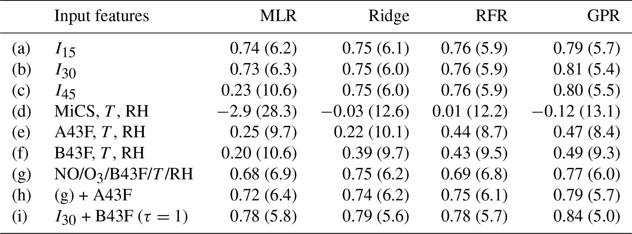
For a first comparison of the calibration performance of the four methods, we show R² scores and RMSEs in Table 2, rows (a) to (c), averaged across all 21 sensor nodes. GPR emerges as the best-performing method for all three sets of predictor choices, reaching R² scores better than 0.8 for I₃₀ and I₄₅. This highlights that GPR should from now on be considered an option in similar sensor calibration exercises. RFR consistently performs worse than GPR but slightly better than ridge regression, which in turn outperforms MLR in all cases, but the differences are fairly small for I₁₅ and I₃₀. A notable exception occurs for I₄₅, where the R² score for MLR suddenly drops abruptly to around 0.2. This sudden performance loss can be understood from the aforementioned curse of dimensionality: MLR increasingly overfits the training data as the number of predictors increases; the existing sample size becomes too small to constrain the 45 regression coefficients (Bishop, 2006; Runge et al., 2012). The machine learning methods can deal with this increase in dimensionality highly effectively and thus perform well throughout all three cases. Indeed, GPR and ridge regression benefit slightly from the additional predictor transformations. This robustness to regression dimensionality is a first central advantage of machine learning methods in sensor calibrations. Machine learning methods will be more reliable and will allow users to work in a higher-dimensional calibration space compared to MLR. Having said that, for 15 input features the performance of all methods appears very similar on first sight, making MLR seemingly a viable alternative to the machine learning methods. We note, however, that there is no apparent disadvantage in using machine learning methods to prevent potential dangers of overfitting depending on sample size.

Table 2 Average NO₂ sensor skill depending on the selection of predictors. Shown are average R² scores and root mean squared errors (in brackets; units µg m⁻³). Results are averaged over the 21 low-cost sensor nodes with 600 hourly training samples each, and the evaluation is carried out for 220 test samples each. RH stands for relative humidity, and T stands for temperature.

3.1.2 Calibration performance depending on sample size

We next consider the performance dependence on sample size of the training data (Fig. 4). The advantages of machine learning methods become even more evident for smaller numbers of training samples, even if we consider case (b) with 30 predictors, i.e. I₃₀, for which we found that MLR performs fairly well if trained on 600 h of data. The mean R² score and RMSE (µg m⁻³) quickly deteriorate for smaller sample sizes for MLR, in particular below a threshold of less than 400 h of training data. Ridge regression – its statistical learning equivalent – always outperforms MLR. Both GPR and RFR can already perform well at small samples sizes of less than 300 h. While all methods converge towards similar performance approaching 600 h of training data (Table 2), MLR is generally performing worse than ridge regression and significantly worse that RFR and GPR.

Further evidence for advantages of machine learning methods are provided in Fig. 5, showing boxplots of the R² score distributions across all 21 sensor nodes depending on sample size (300, 400, 500, 600 h) and regression method. While median sensor performances of MLR, ridge and GPR ultimately become comparable, MLR is typically found to yield a number of poor-performing calibration functions with some R² scores well below 0.6 even for 600 training hours. In contrast, the distributions are far narrower for the machine learning methods: GPR and RFR do not show a single extreme outlier even after being trained on only 400 h of data, providing strong indications that the two methods are the most reliable. After 600 h, one can effectively expect that all sensors will provide R² scores >0.7 if trained using GPR. Overall, this highlights again that machine learning methods will provide better average skill but are also expected to provide more reliable calibration functions through co-location measurements independent of sensor device and the peculiarities of the individual training and test data set.

Figure 4 Error metrics as a function of the number of training samples for I₃₀, as labelled. The figure highlights the convergence of both metrics for the different regression methods as the sample size increases. Note that MLR would not converge for I₄₅, owing to the curse of dimensionality. This tendency can also be seen here for small sample sizes, where MLR rapidly loses performance. Results are averaged over the 21 low-cost sensor nodes with 600 hourly training samples each, and the evaluation is carried out for 220 test samples each.

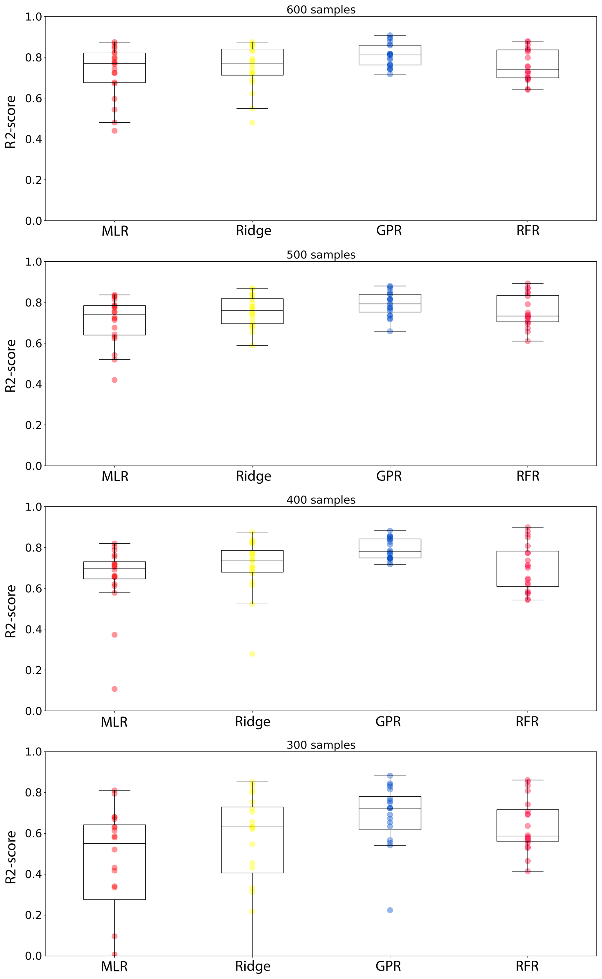
Figure 5 Node-specific I₃₀ R² scores depending on calibration method and training sample size, evaluated on consistent 220 h test data sets in each case (see main text). The boxes extend from the lower to the upper quartile; inset lines mark the median. The whiskers extending from the box indicate the range excluding outliers (fliers). Each circle represents the R² score on the test set for an individual node (21 in total). For MLR, some sensor nodes remain poorly calibrated even for larger sample sizes.

3.1.3 Calibration performance depending on predictor choices and NO₂ device

Tests (a) to (c) listed in Table 2 indicate that the machine learning regressions for NO₂, specifically GPR, can benefit slightly from additional logarithmic predictor transformations but that adding exponential transformations on top of these predictors does not further increase predictive skill, as measured through the R² score and RMSE. Incorporating the logarithmic transformations, we next tested the importance of various predictors to achieve a certain level of calibration skill (rows (d) to (i) in Table 2). This provides two important insights: firstly, we test the predictive skill if we use the individual MiCS and AlphaSense NO₂ sensors separately, i.e. if individual sensors are performing better than others in our calibration setting and if we need all sensors to obtain the best level of calibration performance. Secondly, we test if other environmental influences such as humidity and temperature significantly affect sensor performance.

We first tested three set-ups in which we used only the sensor signals of the two cheaper MiCS devices (d) and then set-ups with the more expensive AlphaSense A43F (e) and B43F (f) devices. Using just the MiCS devices, the R² score drops from 0.75–0.81 for the machine learning methods to around zero, meaning that hardly any of the variation in the true NO₂ reference signal is captured. Using our calibration approach here, the MiCS would therefore not be sufficient to achieve a meaningful measurement performance. The picture looks slightly better, albeit still far from perfect, for the individual A43F and B43F devices for which R² scores of almost 0.5 are reached using non-linear calibration methods. We note that the linear MLR and ridge methods do not achieve the same performance, but ridge outperforms MLR. The most recently developed AlphaSense sensor used in our study, B43F, is the best-performing stand-alone sensor. If we add the $\mathrm{NO}/\mathrm{ozone}$ sensor as well as the humidity and temperature signals to the predictors – case (g) – its performance alone almost reaches the same as for the I₃₀ configuration. This implies that the interference with $\mathrm{NO}/\mathrm{ozone}$, temperature and humidity might be significant and has to be taken into account in the calibration, and if only one sensor could be chosen for the measurements, the B43F sensor would be the best choice. By further adding the A43F sensor to the predictors the predictive skill is only mildly improved (h). Finally, we note that, in this stationary sensor setting, further predictive skill can be gained by considering past measurement values. Here, we included the 1 h lagged signal of the best B43F sensor (i). This is clearly only possible if there is a delayed consistency (or autocorrelation) in the data, which here leads to the best average R² generalization score of 0.84 for GPR and related gains in terms of the RMSE. While being an interesting feature, we will not consider such set-ups in the following, because we intend sensors to be transferable among locations, and they should only rely on live signals for the hour of measurement in question.

In summary, using all sensor signals in combination is a robust and skilful set-up for our NO₂ sensor calibration and is therefore a prudent choice, at least if one of the machine learning methods is used to control for the curse of dimensionality. In particular, the B43F sensor is important to consider in the calibration, but further calibration skill is gained by also considering environmental factors, the presence of interference from ozone and NO, and additional NO₂ devices.

3.2 PM₁₀ sensor calibration

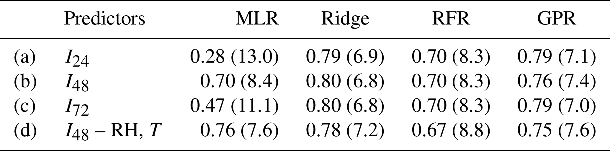
In the same way as for NO₂, we tested several calibration settings for the PM₁₀ sensors. For this purpose, we consider the measurements for the location CarPark, where we co-located three sensors (IDs 19, 25 and 26) with a higher-cost device (Table 1). However, after data cleaning, we have only 509 and 439 samples (hours) for sensors 19 and 25 available, respectively, which our NO₂ analysis above indicates is too short to obtain robust statistics for training and testing the sensors. Instead we focus our analysis on sensor 26 for which there are 1314 h of measurements available. We split these data into 400 samples for training and cross-validation, leaving 914 samples for testing the sensor calibration. Below we discuss results for various calibration configurations, using the 24 predictors for PM₁₀ (Sect. 2.3) and the same four regression methods as for NO₂. The baseline case with just 24 predictors is named I₂₄, following the same nomenclature as for NO₂. I₄₈ and I₇₂ refer to the cases with additional logarithmic and exponential transformations of the predictors according to Eqs. (9a) and (9b). In addition, we test the effects of environmental conditions, as expressed through relative humidity and temperature, by excluding these two variables from the calibration procedure, while using the I₄₈ set-up with the additional log-transformed predictors.

The results of these tests are summarized in Table 3. For the baseline case of 24 non-transformed predictors, RFR (R²=0.70) is outperformed by ridge regression (R²=0.79) and GPR (R²=0.79). This is mainly the result of the fact that some of the pollution values measured with sensor 26 during the test period lie outside the range of values encountered at training stage. RFR cannot predict values beyond its training range (i.e. it cannot extrapolate to higher values) and can therefore not predict those values accurately (see also Zimmerman et al., 2018; Malings et al., 2019). Instead, RFR constantly predicts the maximum value encountered during training in those cases.

Table 3 Sensor skill depending on the selection of predictors for PM₁₀ sensor 26 at location CarPark. Shown are the R² scores and RMSEs (in brackets) evaluated over 914 h of test data, after training and cross-validating the algorithms on 400 h of data. RMSEs are given in µg m⁻³. In (d), relative humidity (RH) and temperature (T) are removed from the calibration variables to test their importance for the measurement skill.

However, this problem is not entirely exclusive to RFR but is inherited by all methods, with RFR only being the most prominent case. We illustrate the more general issue, which will occur in any co-location calibration setting, in Fig. 6. In the training data, there are not any pollution values beyond ca. 40 µg m⁻³, so the RFR predictions simply level off at that value. This is a serious constraint in actual field measurements where one would be particularly interested in episodes of highest pollution. We note that this effect is somewhat alleviated by using GPR and even more so by ridge regression. For the latter, this behaviour is intuitive as the linear relationships learnt by ridge will hold to a good approximation even under extrapolation to previously unseen values. However, even for ridge regression the predictions eventually deviate from the 1:1 line for the highest pollution levels. This aspect will be crucial to consider for any co-location calibration approach, as is also evident from the poor MLR performance, despite being another linear method. In addition, MLR sometimes predicts substantially negative values, producing an overall R² score of below 0.3, whereas the machine learning methods appear to avoid the problem of negative predictions almost entirely. In conclusion, we highlight the necessity for co-location studies to ensure that maximum pollution values encountered during training and testing/deployment are as similar as possible. Extrapolations beyond 10–20 µg m⁻³ appear to be unreliable even if ridge regression is used as calibration algorithm, which is the best among our four methods to combat extrapolation issues.

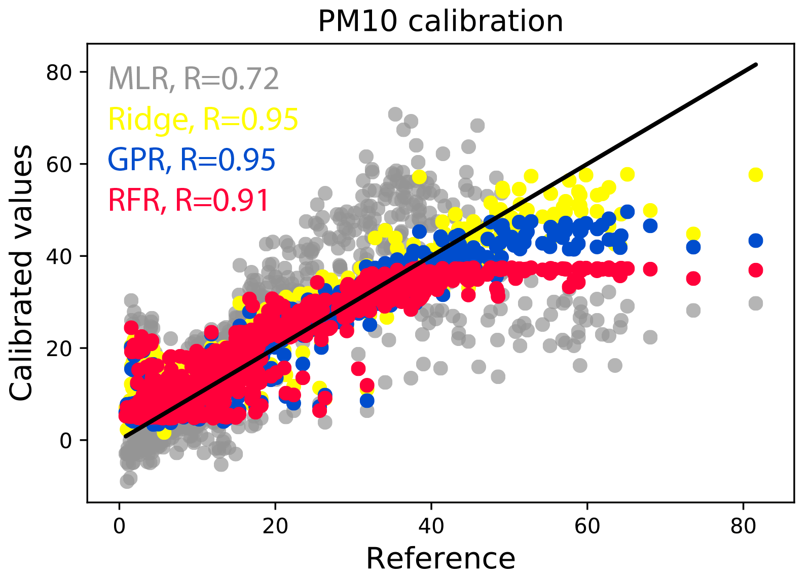
Figure 6 Calibrated PM₁₀ values (in µg m⁻³) versus the reference measurements for 900 h of test data at location CarPark for the I₂₄ predictor set-up. The ideal 1:1 perfect prediction line is drawn in black. Inset values R are the Pearson correlation coefficients.

A test with additional log-transformations (I₄₈) of the predictors led to test score improvements for the two linear methods (Table 3), in particular for MLR (R²=0.7) but also for ridge regression (R²=0.8). This implies that the log-transformations have helped linearize certain predictor–predictand relationships. Further exponential transformations (I₇₂) and thus also further increasing the predictor dimensionality did not lead to an improvement in calibration skill. We therefore ran one final test using the I₄₈ set-up but without relative humidity and temperature included as predictors. This test confirmed that the sensor signals indeed experience a slight interference from humidity and temperature, at least considering the machine learning regressions. Notably, this loss of skill is not observed for MLR for which the R² score actually improves. A likely explanation for this behaviour is the curse of dimensionality that affects MLR more significantly than the three machine learning methods, so the reduction in collinear dimensions (given the sample size constraint) is more beneficial than the information gained by including temperature and humidity in the MLR regression.

In summary, we have found that ridge regression and GPR are the two most reliable and high-performing calibration methods for the PM₁₀ sensor. We are able to attain very good R² scores >0.7 for all four regression methods though. An important point to highlight is the characteristics of the training domain, in particular of the pollution levels encountered during the training data measurements. If the value range is not sufficient to cover the range of interest for future measurement campaigns, then ridge regression might be the most robust choice to alleviate the underprediction of the most extreme pollution values. However, the power of extrapolation of any method is limited, so we underline the need to carefully check every training data set to see if it fulfils such crucial criteria; see also similar discussions in other calibration contexts (Hagan et al., 2018; Zimmerman et al., 2018; Malings et al., 2019).

3.3 Site transferability

Finally, we aim to address the question of site transferability, i.e. how reliably a sensor calibrated through co-location can be used to measure air pollution at a different location. One of the sensor nodes (ID 19) was used for NO₂ measurements at both locations, CR7 and CR9, and was also used to measure PM₁₀ at CR9 and CarPark, allowing us to address this question for our methodology. Note that these tests also include a shift in the time of year (Table 1), which has been hypothesized to be one potentially limiting factor in site transferability. The results of these transferability tests for PM₁₀ (from CR9 to CarPark and vice versa) and NO₂ (from CR7 to CR9 and vice versa) are shown in Figs. 7 and 8, respectively.

For PM₁₀, we trained the regressions, using the I₂₄ predictor set-up, on 400 h of data at either location. This emulates a situation in which, according to our results above, we limit the co-location period to a minimum number of samples required to achieve reasonable performances across all four regression methods. To mitigate issues related to extrapolation (Fig. 6), we selected the last 400 h of the time series for location CarPark (Fig. 7a) and hours 600 to 1000 of the time series for location CR9 (Fig. 7b). This way we still emulate a possible minimal scenario of 400 consecutive hours of co-location, while also including near maximum and minimum pollution values within our training data (given the available measurement data). We note that alternative sampling approaches, such as random sampling with shuffling of the data, could lead to artificial effects at validation and testing stages because of autocorrelation effects that could inflate apparent calibration skill. The maximum pollution found within the two time slices differ only by ca. ±10 µg m⁻³, for which at least ridge regression should provide reasonable extrapolation performances. For the resulting predictions at location CarPark, using models trained on the CR9 data, we achieve generally very good R² scores ranging between 0.67 for RFR and 0.78 for ridge regression. The site-transferred measurement performance of sensor 19 is therefore almost as good as the one for sensor 26 at the co-location site itself (Table 3); i.e. we cannot detect any significant loss in measurement performance due to the site transfer. A surprising element is that MLR performs almost as good as ridge regression in this case, whereas it performed poorly for sensor 26, where it only achieved an R² score of 0.28 (Table 3). This underlines our previous observation that the performance of MLR is more sensitive to the specific sensor hardware, with sometimes low performance for relatively small sample sizes (Fig. 5). However, our results also show again that linear methods appear to generally perform well for our PM₁₀ sensors, with ridge regression being the most reliable and high-performing choice overall. These results are further supported by calculations concerning the detection of only the most extreme pollution events in the time series; see also the definition of such events described in the caption of Fig. 7. We characterize such events in the form of their statistical recall in our sensor measurements (the fraction of extreme pollution events in the reference time series that are also identified by our calibrated sensors) and precision (the fraction of extreme events identified by our sensors that are indeed also extreme events in the reference time series) and show the results as inset numbers in Figs. 7 and 8. Overall, these site-transfer PM₁₀ results from CR9 to CarPark imply that sensors calibrated through co-location can achieve high measurement performance distant from the co-location site.

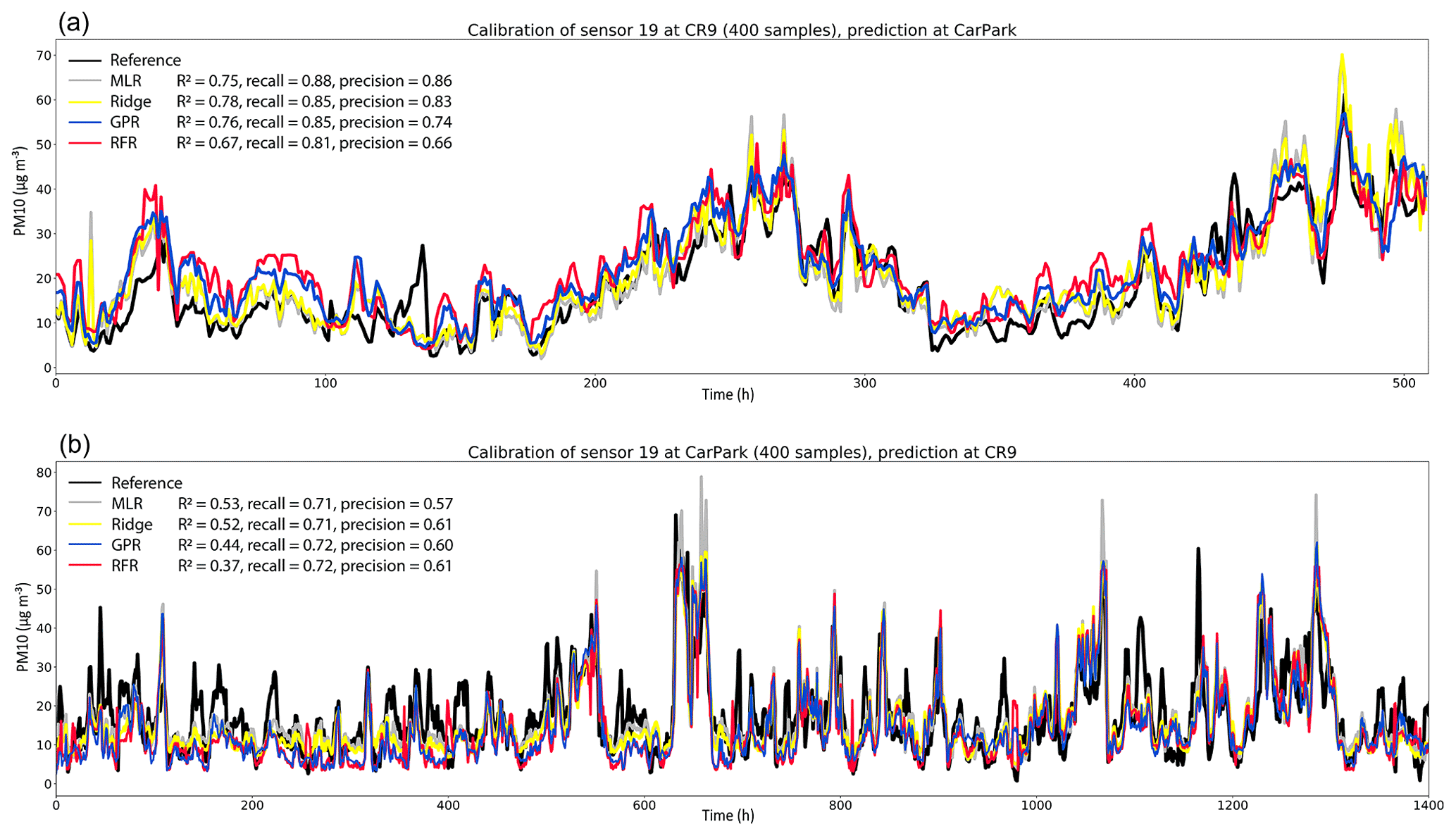
Figure 7 Tests of PM₁₀ sensor site transfers using calibration models trained on 400 h of data. (a) Predictions for the four regression models (as labelled) and reference measurements at location CarPark, using models trained at CR9, and (b) at location CR9, using models trained on data measured at CarPark. The inset values provide the R² scores for each method relative to the reference as well as the corresponding recall and precision for the detection of the strongest pollution events, which are typically of particular interest in real-life situations (here defined as events when two values within the last 3 h exceeded a threshold of 35 µg m⁻³). For compactness, we only show data for times at which both reference and low-cost sensor data were available, and we label these hours as a consecutive timeline.

However, we do find that site transferability is not always as straightforward as found for this particular case. For example, for the inverse transfer using models trained at CarPark and predicting PM₁₀ pollution levels at CR9, we find lower R² scores overall. There is consistency in the sense that MLR and ridge remain the best performing methods for sensor 19 with R² scores of around 0.5, but the sensors now miss several significant pollution events in the time series. We note, however, that many of the most extreme pollution events are still detected, which is evident from the still relatively high precision and recall scores for all methods. These results underline that, in general at least, a good performance can be achieved with co-location calibrations but that there are also significant challenges posed by site transfers. In particular, the problem is not necessarily symmetric among sites, i.e. the skill of the method can depend on the direction of the transfer, even if the pollution levels at both sites are similar. We therefore hope that our insights and results will motivate further work in this direction, with the aim to identify possible causes of such effects. We discuss some of the possible reasons for this behaviour in Sect. 4.

Figure 8 Tests of NO₂ sensor site transfers using calibration models trained on all available samples for locations CR7 and CR9. (a) Predictions for the four regression models (as labelled) and reference measurements at location CR7, using models trained on data from CR9 and (b) vice versa. The inset values provide the R² scores for each method relative to the reference as well as the corresponding recall and precision for the detection of the strongest pollution events, which are typically of particular interest in real-life situations. Since the two locations were subject to very different pollution ranges (note the different value ranges on the y axes), these are defined in (a) as 45 µg m⁻³ and in (b) as 90 µg m⁻³, and we indicate these thresholds by grey dashed lines. An extreme pollution event occurs when the threshold is exceeded for 2 of the last 3 h. For compactness, we only show data for times at which both reference and low-cost sensor data were available, and we label these hours as a consecutive timeline.

Similarly, we find promising results for the NO₂ sensor site transfer using the I₃₀ predictor set-up (Fig. 8). The key challenge for the sensor transfer from CR7 to CR9 is that the maximal pollution levels at the two locations differ substantially, with peak concentration being around 100 µg m⁻³ greater at CR9. To allow for the best possible learning opportunities for the regression algorithms, we therefore used all available samples for training, which are 1482 samples at CR9 and 829 samples at CR7. This leads to overall good performance of the non-linear RFR and GPR methods at location CR7 using models trained at CR9. As no extrapolation is necessary, these methods achieve a good performance of R² scores >0.6 and also a good balance of precision and recall. The results are, however, slightly worse than for the same site calibrations (Table 2). Ridge regression has a tendency to overpredict NO₂ pollution levels in this particular case, likely because it cannot capture some non-linear effects that would have limited the prediction values. As a result, it also reproduces almost all extreme pollution events where the concentration of NO₂ exceeds 45 µg m⁻³ (recall =0.98) but also predicts many false pollution events (precision =0.49).

Despite the large sample size, MLR performs poorly for both site transfers (R²=0.07 and −0.31). In particular, MLR underpredicts, sometimes providing even impossible negative pollution estimates at CR7, whereas it provides several runaway positive values at CR9 (Fig. 8). However, at CR9 all methods struggle with the impossible challenge of extrapolation far outside their training domain, which effectively is an extreme demonstration of the effects of an ill-considered training range (cf. Fig. 6). Among the machine learning methods, the effect is as expected most prominent for RFR (R²=0.36), which cannot predict any pollution values beyond those encountered at training stage. This is a serious limitation and means that the method scores nil on precision and recall of any extreme pollution events at CR9 where NO₂ levels exceeded 90 µg m⁻³. GPR is slightly better at extrapolating beyond its training domain (compare also Fig. 6) but still not good enough to reproduce any of the extreme pollution events, giving rise to equally low precision and recall. Ridge regression, as a regularized linear method, performs best in the sense that it is able to reproduce at least a few of the extreme events (recall =0.05) and predicting no false extreme events (precision =1.0), while still achieving an R² score of 0.53. Nonetheless, it is clear from the time series in Fig. 8 that none of the regression methods works for this site transfer, simply because of the too large extrapolation range.

4 Discussion and conclusions

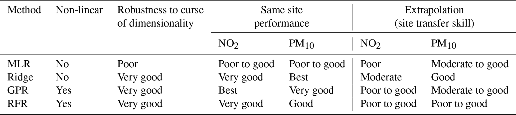
We have compared four different regression methods to calibrate a number of low-cost NO₂ and PM₁₀ sensors against reference measurement signals, by means of co-location at three separate sites in London, UK. A summary of the various features of each regression algorithm is given in Table 4. Comparing the four regression methods, our main conclusions are the following:

1. For the 21 NO₂ sensor nodes, Gaussian process regression (GPR) is generally performing best at the same measurement site, followed by ridge regression, random forest regression (RFR), and multiple linear regression (MLR). For a single sensor PM₁₀ calibration, we find that ridge regression and GPR attain about the same measurement performance, with a slight edge for ridge regression. We note that in particular the relative performance of GPR differs greatly from a recent study by Malings et al. (2019), likely due to our different choice of kernel design.

2. Special care must be taken of the calibration conditions, in particular if sensors are thereafter used for measurements in areas where higher pollution levels are to be expected. The linear ridge method can best mitigate the catastrophic measurement failure in such extrapolation settings, for both NO₂ and PM₁₀ measurements, but also fails if measurement signals deviate by more than around 10–20 µg m⁻³ from the maximum pollution level in the training data. For our NO₂ measurement with site transfer, we find that the non-linear methods, GPR and RFR, can outperform ridge regression, assuming that the training pollution range encapsulates the range of values encountered at the new site. For the PM₁₀ sensor calibrations and corresponding site transfers, we find that ridge regression is the highest performing and most reliable calibration algorithm overall.

3. All three machine learning methods (ridge, GPR and RFR) generally outperform or perform as least as good as MLR. The machine learning methods are also more reliable if many signals are used for calibration, or if the number of measurement samples is relatively small. MLR suffers most significantly from the curse of dimensionality in those settings and can produce highly erroneous results.

4. Under careful consideration of the calibration conditions, given expected measurement conditions, the low-cost sensors typically achieve high performances with R² scores often exceeding 0.8 on new unseen test data.

Table 4 Summary and qualitative evaluation of key features of each of the four regression algorithms. The robustness to the curse of dimensionality refers to how well each algorithm can handle an increase in the number of calibration variables. In addition, we summarize how well each method performs for our calibrations here if evaluated against test data sampled at the same site as the one used for training and after site transfers. The variable performance of GPR (and also RFR) for site transfers is mainly the result of its limited skill to extrapolate so that its performance will always depend strongly on how representative the training data is in terms of value ranges. We also note that robustness to the curse of dimensionality (third column) is only considered with respect to the maximum of 72 predictors considered here. In even higher dimensions more significant differences across the machine learning methods are expected to occur eventually.

On another note, we highlight that we sometimes found significant signals in our test data sets that were not reproduced by our low-cost sensor nodes (see, for example, the pollution spike at t≈140 in Fig. 7a) even if the measured pollution value lies well within the training data range. It is hard to assign reasons to this surprising sensor behaviour, as our low-cost sensors are apparently able to capture most of the other pollution spikes well for the same data set. One possible reason is a calibration blind spot; i.e. we encounter a new type of sensor interference which we did not find in the training data. For example, this could be substantial changes in environmental conditions or, for example, PM composition, which are not captured by the calibration function. In our interpretation of results, this would represent again an extrapolation with respect to the predictors and/or the predictands. However, we think that this is unlikely, given that the behaviour is not found frequently, at least in this particular time series. Two other options are (a) imperfect co-location (e.g. we might have missed an important local pollution plume by chance) or (b) temporary sensor failures that were removed by the MAD outlier removal, i.e. that our sensors were temporarily inoperable at the time of a pollution spike that dominated the values for the given measurement hour. Interesting aspects to explore as part of future work might be to compare how sensitive site transfer performances are to the measurement principle of the NO₂ and PM₁₀ devices used and effects of the seasonal cycle (e.g. winter-based calibrations to be used during summer). We hope that future measurement campaigns can provide further insights into such calibration challenges, and we hope that our study can motivate further work in this direction.

In conclusion, our results underline the potential of machine learning algorithms for the calibration of co-located low-cost NO₂ and PM₁₀ sensors. At the same time, we highlight several significant challenges that will always have to be considered in similar calibration processes. This includes the need for a well-adjusted calibration data set to avoid calibration failure if the algorithm needs to extrapolate to significantly higher pollution values and the role of individual choices relating to the combination of calibration variables and calibration algorithms, e.g. concerning the curse of dimensionality, predictor transformations and linearity in the predictor–predictand relationships. Recent studies indicate that the issues related to extrapolation can be mitigated through the application of hybrid models in which non-linear machine learning models are used within the training domain and a simpler linear regression approach otherwise (Hagan et al., 2018; Malings et al., 2019). We note that in particular ridge regression could be a good compromise, which does not require a somewhat arbitrary hybrid-model definition. Having said that, we also found that even high-dimensional linear methods have ultimately limited extrapolation skill (Fig. 6), so the consideration of the training data pollution range remains of fundamental importance. We hope that such insights will contribute to ever less expensive and more spatially dense measurements of air pollution in the future and that our work will motivate additional measurement campaigns, testing of other calibration algorithms and further low-cost sensor development.