Controlled-release experiment to investigate uncertainties in UAV-based emission quantification for methane point sources

Mapping trace gas emission plumes using in situ measurements from unmanned aerial vehicles (UAVs) is an emerging and attractive possibility to quantify emissions from localized sources. Here, we present the results of an extensive controlled-release experiment in Dübendorf, Switzerland, which was conducted to develop an optimal quantification method and to determine the related uncertainties under various environmental and sampling conditions. Atmospheric methane mole fractions were simultaneously measured using a miniaturized fast-response quantum cascade laser absorption spectrometer (QCLAS) and an active AirCore system mounted on a commercial UAV. Emission fluxes were estimated using a mass-balance method by flying the UAV-based system through a vertical cross-section downwind of the point source perpendicular to the main wind direction at multiple altitudes. A refined kriging framework, called cluster-based kriging, was developed to spatially map individual methane measurement points into the whole measurement plane, while taking into account the different spatial scales between background and enhanced methane values in the plume. We found that the new kriging framework resulted in better quantification compared to ordinary kriging. The average bias of the estimated emissions was −1 %, and the average residual of individual errors was 54 %. A Direct comparison of QCLAS and AirCore measurements shows that AirCore measurements are smoothed by 20 s and had an average time lag of 7 s. AirCore measurements also stretch linearly with time at an average rate of 0.06 s for every second of QCLAS measurement. Applying these corrections to the AirCore measurements and successively calculating an emission estimate shows an enhancement of the accuracy by 3 % as compared to its uncorrected counterpart. Optimal plume sampling, including the downwind measurement distance, depends on wind and turbulence conditions, and it is furthermore limited by numerous parameters such as the maximum flight time and the measurement accuracy. Under favourable measurement conditions, emissions could be quantified with an uncertainty of 30 %. Uncertainties increase when wind speeds are below 2.3 m s⁻¹ and directional variability is above 33^∘, and when the downwind distance is above 75 m. In addition, the flux estimates were also compared to estimates from the well-established OTM-33A method involving stationary measurements. A good agreement was found, both approaches being close to the true release and uncertainties of both methods usually capturing the true release.

1 Introduction

Methane emissions from localized sources such as oil- and gas-production facilities are often caused by leakage giving rise to highly uncertain emission fluxes with high spatial and temporal variability (Kemp et al., 2016; Fox et al., 2019). A significant disparity was observed, for example, between facility-observed bottom-up emission inventories and a more traditional component-based emission inventory (Brandt et al., 2014; Alvarez et al., 2018). Observation-based estimates from the United States indicate that emissions from oil and gas are underestimated in official emission inventories (Alvarez et al., 2018; Omara et al., 2018; Zhang et al., 2020). Further measurements of leakage rates from oil- and gas-production facilities in other regions of the world, such as those conducted during the ROmanian Methane Emissions from Oil and gas (ROMEO) measurement campaign in Romania (Röckmann and the ROMEO team, 2020), are therefore essential to validate and improve current estimates.

A broad range of methods of methane emission quantification for facility-scale sources has been developed, which includes ground-based thermal imaging (Gålfalk et al., 2016), aircraft remote sensing (Frankenberg et al., 2016; Kuai et al., 2016; Thorpe et al., 2016), chamber sampling (Kang et al., 2014; Yver Kwok et al., 2015), ground-based tracer-release correlation (Lamb et al., 2015, 2016; Omara et al., 2016; Roscioli et al., 2015; Feitz et al., 2018; Fjelsted et al., 2020) and Gaussian plume matching (Ars et al., 2017; Bakkaloglu et al., 2021). Some of these methods, for example, tracer-release correlation, are quite accurate but expensive, intrusive, and time-consuming, while other methods suffer from large, poorly quantifiable uncertainties.

An emerging and attractive approach to quantify emissions from point sources, or more generally from spatially localized sources, involves deploying integrated unmanned aerial vehicle (UAV) systems capable of measuring atmospheric trace gas concentrations. The most common ways of measuring methane from UAVs include (1) collection of ambient air samples using onboard storage equipment and subsequent analysis of the samples with instrumentation on the ground (Chang et al., 2016; Greatwood et al., 2017; Andersen et al., 2018), (2) live analysis of air samples pumping air into a long tube connected to a ground-based analyser (Brosy et al., 2017; Shah et al., 2019), and (3) in situ reporting of measurements using an analyser mounted on the UAV (Berman et al., 2012; Nathan et al., 2015; Golston et al., 2017; Martinez et al., 2020; Tuzson et al., 2020). Small UAVs with payloads of a few kilograms are affordable, versatile, and much more easy to deploy compared to larger UAVs or aircraft. UAVs allow the plume to be transected over its entire vertical and horizontal extent, which reduces the dependence on assumptions on horizontal and vertical dispersion compared to ground-based mobile or stationary measurements that only capture a small portion of the plume.

Although UAV-based methane measurements are gaining popularity, systematic studies on testing and comparing different quantification methods and analysing the different sources of uncertainty are still sparse (Golston et al., 2018; Yang et al., 2018; Shah et al., 2019; Hollenbeck et al., 2021; Shaw et al., 2021). The main goal of this study is to develop an improved strategy to quantify local methane sources using UAV measurements and to test this strategy on UAV measurements obtained downwind from sources with known fluxes. It is crucial to test a new quantification technique with a set of sources with a known release before applying the technique to sources with unknown emissions (Feitz et al., 2018; Shah et al., 2020). To this end, we designed the MethAne Release Experiment (MATRIX), where a series of controlled and partly blind methane releases were performed from 9 February to 14 March 2020 in Dübendorf, Switzerland. Methane mole fractions were measured using a UAV-based sensor (Tuzson et al., 2020) and an active AirCore system (Andersen et al., 2018). Adopting the mass-balance approach, the UAV was flown downwind of the source perpendicular to the main wind direction at different vertical levels to derive emission fluxes. In this study, we describe a novel quantification approach and report on its capability to reproduce known emissions. Furthermore, we investigate this approach and its sensitivity to different measurement configurations and provide recommendations for an optimal sampling.

The new UAV-based quantification approach presented here was developed to support the ROMEO campaign that took place in September and October 2019. With 415.60 kt CH₄ yr⁻¹, Romania has one of the highest per-capita methane emissions from the energy sector in the European Union, according to the latest UNFCCC 2018 report. This emission estimate was mainly derived using prescribed Tier 1 emission factors following the IPCC guidelines for national reporting, which are both non-country-specific and quite uncertain. The ROMEO campaign was, thus, put into action to investigate the accuracy of this estimate. Eight ground measurement teams, including our UAV system, were deployed to quantify methane emissions from over 1000 oil- and gas-production facilities (Röckmann and the ROMEO team, 2020). Reported emissions from UAV-based measurements collected in the western region of Wallachia, Romania, during the ROMEO campaign were generated using the quantification approach developed in this study.

In this paper, we give first an overview of the instruments used in the controlled-release experiment (Sect. 2), followed by the details regarding the setup of the experiments and the mass-balance approach in Sect. 3. The data treatment and interpolation schemes applied to the measurements of both methane and wind are discussed in Sect. 4. Quantification results from the controlled-release experiments are presented in Sect. 5.

2 Instruments

The in situ measurements of atmospheric CH₄ mole fractions were performed using two different techniques: (i) a lightweight laser absorption spectrometer and (ii) an active AirCore system. These devices were mounted beneath a commercial hexacopter (Matrice 600, DJI), equipped with an RTK-GPS receiver (NEO-M8P-2, SparkFun) for accurate positioning of the UAV in all three dimensions. The integrated system, illustrated in Fig. 1, weighs about 13 kg, of which the payload is around 3 kg and can have a maximum flight time of 20 min.

Figure 1 The embedded UAV system used for CH₄ detection: the QCLAS analyser and the active AirCore sampling system are mounted below a Matrice 600 DJI hexacopter equipped with an RTK-GPS system.

2.1 Quantum cascade laser spectrometer (QCLAS)

The in situ airborne analyser, developed at Empa, is a compact and lightweight mid-IR laser absorption spectrometer (Graf et al., 2018; Tuzson et al., 2020) capable of measuring atmospheric methane mole fractions at 1 s time resolution. The instrument achieves a precision (1σ) of 1.1 ppb at 1 s and 0.1 ppb at 100 s averaging time. This performance is also mainly preserved under flight conditions. The analyser has a compact footprint ($\mathrm{15}\times \mathrm{45}\times \mathrm{25}$ cm³) and weighs only 2.1 kg, including batteries.

The analyser uses a distributed feedback (DFB) quantum cascade laser (QCL) emitting in the mid-infrared at 7.83 µm. During the flight, air flows passively through an open circular absorption cell of 77 mm radius. Multiple reflections of the laser beam on the segmented inner surface result in an effective optical path of about 10 m. The compact design of the multipass cell combines the advantage of a long optical path with mechanical stability, allowing for efficient and interference-free beam folding (Graf et al., 2018).

The energy consumption of the spectrometer has been minimized using a customized system-on-chip (SoC) FPGA-based hardware control and data acquisition as well as a custom-made laser driving electronics (Liu et al., 2018). The instrument's precision, linearity, and calibration were characterized and consequently validated under field conditions (Tuzson et al., 2020). Briefly, the instrument was calibrated by inserting it into a custom-built small-volume (60 L) climate chamber. This chamber was then hermetically sealed and continuously purged with a certified calibration gas with high CH₄ concentration (200 ppm±1 %; PanGas, Switzerland). Furthermore, the gas was dynamically diluted with dry nitrogen (N₂) in a stepwise fashion using calibrated mass flow controllers. The overall uncertainty was estimated to be ±2 %. Repeated experiments showed that the instrument preserves its linearity, and only a marginal drift may appear in the offset. This, however, is fully accounted for when applying the background CH₄ subtraction step (see Sect. 4.4). Real-time data synchronization between the instrument and a computer on the ground is made possible by a wireless bidirectional data link (SkyHopper PRO). This allows for real-time access to the raw spectra and all hardware parameters during the flights, which enables the operator to do real-time spectral fitting and logging. Thus, the operator is provided with full control of the hardware, continuous monitoring of the instrument's status, and in situ monitoring of the ambient CH₄ values during the flights.

2.2 Active AirCore

The active AirCore, designed for atmospheric sampling on a UAV, consists of 50 m thin-wall stainless-steel tubing, a dryer, a micro-pump, and a data logger (Andersen et al., 2018). The whole system is enclosed in a carbon fibre box with a compact footprint (1.1 kg, $\mathrm{34}\times \mathrm{19.5}\times \mathrm{12.0}$ cm³) making it suitable for UAV-based measurements.

Prior to each quantification flight, the active AirCore is flushed with a calibrated fill gas and spiked with about 10 ppm CO, in order to identify the starting point of ambient air sampling. Shortly before the integrated UAV system takes off, the micro-pump is turned on to sample ambient air, and immediately after the quantification flight, it is turned off to stop sampling ambient air. The active AirCore samples are then consequently analysed on site with a trace gas analyser (cavity ring-down spectroscopy (CRDS) G2401-m, Picarro, Inc., CA, USA). The precision (1σ, 0.25 Hz) of the CRDS analyser was determined to be better than 0.7  ppb. A single-point calibration was used to correct the potential drift of the CRDS measurements. Measured methane mole fraction obtained using the AirCore system was linked to a known calibration standard that is traceable to the WMO X2004A CH₄ scale (Vinkovic et al., 2022)

2.3 RTK-GPS system

Readily available commercial UAVs, including the Matrice 600 DJI, rely on a simple global positioning system (GPS), similar to systems found in other utilities such as mobile phones and smart watches. GPS readings combined with ambient pressure measurements are used to obtain the spatial coordinates, specifically the altitude, of the UAV at the time of flight. Manufacturer specification reports vertical accuracy of this type of UAVs to be ±0.50 m. However, this level of accuracy is not sufficient for our purpose that requires a precise spatial mapping of the plumes, especially with respect to height.

Alternatively, real-time kinematic (RTK) positioning can be employed to enhance positioning accuracy. Nowadays, accuracy at the level of centimetres is possible, even with low-cost receivers (such as the NEO-M8P), by capturing measurements of carrier phase signals from the GPS satellites and then post-processing the logs with open-source programs (e.g. RTKLIB). For our purpose, we deployed two RTK-GPS boards from SparkFun. The rover was integrated with the data acquisition of the UAV-based QCLAS system, while the second board was deployed as a stand-alone, battery-powered base station. Post-processing of raw data was done using RTKLIB, which returns corrected coordinates.

A direct comparison of an altitude time series between the UAV-GPS and the RTK-GPS data in one of our flights is presented in Fig. 2. Quantified average drift of the UAV-GPS for the entire duration of the controlled-release experiment was found to be 0.1 cm s⁻¹, equivalent to 0.6 m of altitude drift for a 10 min duration measurement flight. Details on how this altitude drift affects our quantification estimate are discussed in Sect. 5.1.1

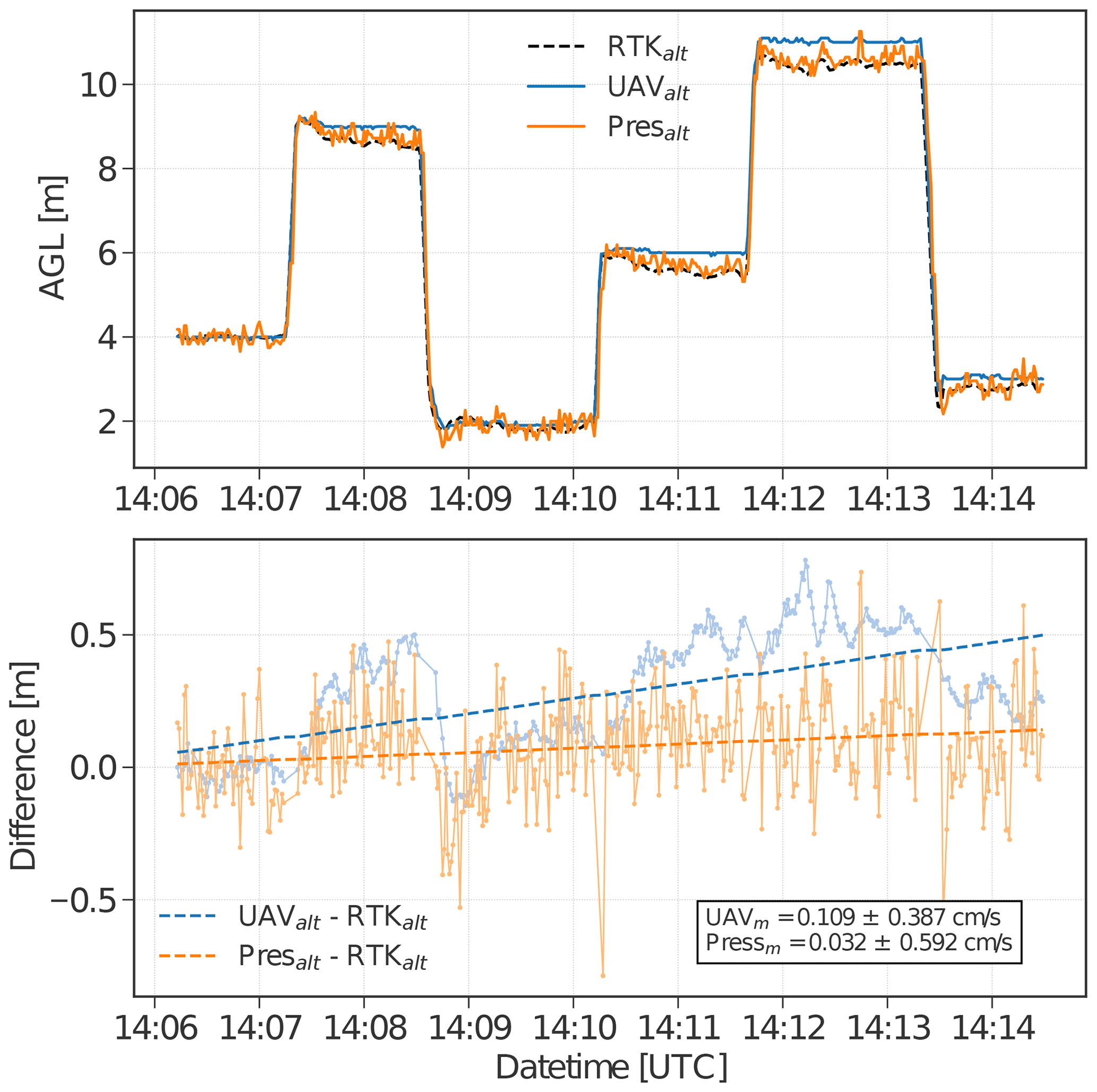
Figure 2 Recorded altitude during the flight with code 314_03. Colour-coded lines represent the altitude measured using three different systems. The dashed black line and blue line correspond to the altitude recorded by RTK and UAV-GPS, respectively. The orange line refers to the altitude derived using the pressure sensor. Dashed blue and orange lines are fits representing a linear regression, with the subscript m referring to the slope of the line.

3 Controlled-release experiment

The release experiment was performed over a managed agricultural field (Agrar Hauser) near the city of Dübendorf, Switzerland. The field is a seasonal cropland with an access road mainly used by pedestrians and bikers. The location is relatively flat but is shielded by a forested hill about 250 m in the south. The release experiment was performed from 23 February to 14 March 2020 with a total of 9 d of active measurements. There is no livestock or other significant methane source in the vicinity of the field, making it an ideal location for the experiment. The selection of active days was mainly based on favourable weather conditions, i.e. days with no precipitation and a sufficiently large wind speed but smaller than 8 m s⁻¹, which is the maximum value given by the UAV flight specifications. Local wind speeds during the selected days ranged from 1–7 m s⁻¹. A total of 35 measurement flights were performed during the whole campaign, out of which 18 are suitable for quantification. The rest had to be discarded mainly due to technical problems with either the UAV, the analysers, the controlled release, or the GPS device. A sample measurement flight is presented in Fig. 3, which also provides an aerial view of the site.

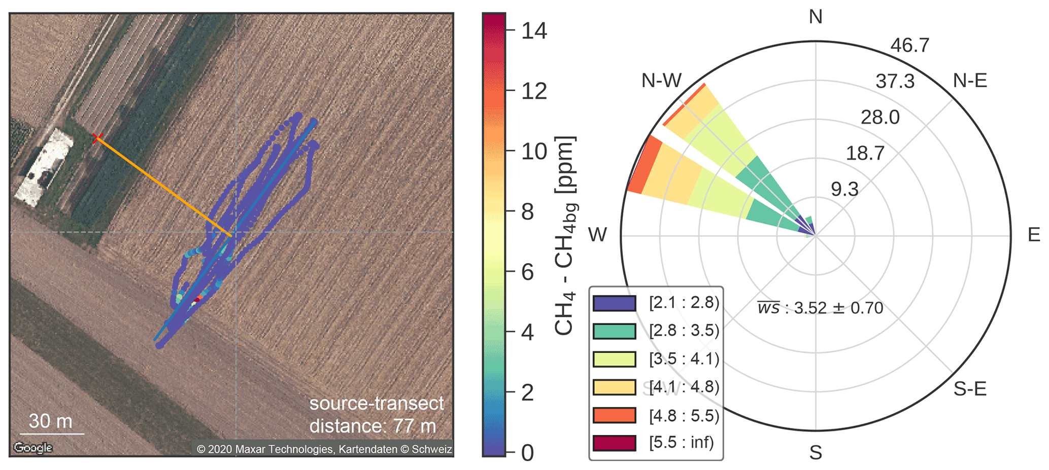
Figure 3 Measured methane mole fraction above background during MATRIX with flight code 312_03 and its corresponding wind rose. The red cross indicates the location of the artificial source. The source transect distance, shown as the orange line, is computed as the perpendicular distance between the source and the measurement plane. The flight trajectories are illustrated as coloured dots, indicating the measured local CH₄ concentrations. Wind and turbulence conditions are measured with a 3D sonic anemometer located next to the source.

Alongside the UAV flights, a second quantification method based on stationary measurements with an independent methane analyser was applied on the first 3 d of the campaign for comparison. The method, called OTM-33A (Thoma et al., 2012), is presented in more detail in Sect. 4.2. In order to avoid any possible bias in the data processing towards the real controlled release, two of the releases were conduced as blind experiments, where a third-party person released methane at a rate not known to the team.

An artificial methane source, in the form of natural gas of which 92.2 % is CH₄, was released from a 50 L high-pressure cylinder. The gas was directed through a 100 m long 1.2 cm inner diameter tubing to the release point. The end of the tubing was placed at about 1.5 m above surface. A mass flow controller (MFC; red-y series, Vögtlin Instruments) calibrated for methane up to 100 L min⁻¹ at normal conditions was used to regulate the gas release. A summary of the release rates during the experiment is given in Table 1. The release rates used in this study are a good representation of emissions from normal operating (i.e. excluding super-emitters) natural gas production sites in the United States which produce 0.13–0.58 g s⁻¹ (Omara et al., 2018). At the start of each measurement day, a suitable location of the release was determined based on prevailing winds. Meteorological conditions were measured using 3D (uSonic-3 Scientific, METEK) and/or 2.5D (TriSonica Mini, Anemoment) anemometers, which were usually placed next to the release point of the source. Stability classes listed in Table 1 were determined by calculating a dimensionless height, $\mathit{\zeta }=z/L$, where z is the height of wind measurement, and L is the Obukhov length. The dimensionless height is used as a stability parameter, where ζ<0 indicates unstable, ζ>0 unstable, and ζ=0 for neutral conditions.

Table 1 Overview of MethAne Release Experiment (MATRIX).

Instruments – A: AirCore, Q: QCLAS, O: OTM-33A, R: RTK. Meteorological stability – N: Neutral, U: Unstable, S: Stable.

4 Method

4.1 Mass balance

Mass-balance methods have been applied extensively to aircraft-based measurements for quantifying emissions from facility scale (e.g. Ryerson et al., 2001; Karion et al., 2013; Gordon et al., 2015; Lavoie et al., 2015; Tadić et al., 2017) up to urban and regional scale (e.g. Cambaliza et al., 2015; Pitt et al., 2019; Fiehn et al., 2020; Klausner et al., 2020). The quantification involves flying downwind and/or around a region of interest at a single vertical height or multiple heights. Emission rates are quantified by taking the net difference between fluxes into and out of a volume containing the source. Subtracting a large-scale background, the inflow is usually assumed to be zero, and the outflow is determined from the enhancements above background inside the plume downwind of the source, together with measurements or model assumptions of wind speed. With the advent of UAVs, estimating emissions using the cross-sectional mass-balance method originally used for aircraft may be adapted to smaller scale and more localized sources. Emission quantification is best performed by flying the UAV downwind of a given source perpendicular to the main wind direction at multiple altitudes above ground up to an altitude, z_max, where no discernible change in methane mixing ratio is observed. Background mole fractions can be determined from measurements outside of the plume or from measurements upwind of the source.

Applying mass conservation for a chemically non-reactive gas within a control volume, the emission flux downwind of a given source can be quantified as

$$\begin{array}{}\text{(1)}& Q_{\mathrm{c}}=\underset{y_{\min }}{\overset{y_{\max }}{\int }}\underset{\mathrm{0}}{\overset{z_{\max }}{\int }}c(y,z)\mathit{u}(y,z)\cdot \widehat{\mathit{n}}\mathrm{d}z\mathrm{d}y,\end{array}$$

where Q_c is the sum of methane emission fluxes within the area of interest. The y axis is aligned with the vertical cross-section in which the UAV is flown. The integral over this two-dimensional plane is approximated in the observations as a discrete summation of the product of the mass concentration of methane above background c(y,z) and the component of the horizontal wind vector u(y,z) normal to the vertical cross-section, i.e. parallel to the unit vector $\widehat{\mathit{n}}$. In doing so, it is assumed that there are no other significant sources of methane emissions upwind besides the controlled release.

4.2 OTM-33A

The other test method (OTM) 33A was introduced by Thoma et al. (2012) to quantify emissions from natural oil and gas sites emitting at near-ground level without having the need to access the site. This approach heavily relies on the assumption that plume dispersion is governed by the point source Gaussian (PSG) model and thus requires certain conditions to be met for effective quantification. In particular, the target source must come from a single point, and no nearby sources should contribute to the measurement. Furthermore, no obstacle should be present between the source and the measurement point. Lastly, measurements of methane and meteorological parameters should be collected at 1–2 Hz and should be taken under rather steady wind conditions with a wind speed of at least 1 m s⁻¹ blowing consistently from the source to the measurement point over a period of at least 15–20 min.

The emission rate, Q_c, of the point source is then estimated using the following equation that is based on spatial integration over a Gaussian shaped plume of horizontal width σ_y and vertical width σ_z:

$$\begin{array}{}\text{(2)}& Q_{\mathrm{c}}=\mathrm{2}\cdot \mathit{\pi }\cdot {\mathit{\sigma }}_y\cdot {\mathit{\sigma }}_z\cdot \stackrel{\mathrm{‾}}{U}\cdot C_{\mathrm{peak}}.\end{array}$$

The horizontal and vertical dispersion coefficients σ_y and σ_z are parameterized as a function of distance from the source using a lookup table developed by Thoma et al. (2012) based on Pasquill stability classes. The average wind speed during the measurements is $\stackrel{\mathrm{‾}}{U}$, and the C_peak is obtained by taking the peak of a Gaussian fit of methane enhancements with respect to wind directions, binned into 10^∘.

The method was characterized using controlled-release experiments (Brantley et al., 2014; Robertson et al., 2017; Edie et al., 2020), which suggested that the method has a 2σ error of ±70 % with a slight negative bias of about 5 % (Heltzel et al., 2020). It was eventually used to quantify emissions from oil and gas plants in the United States (Brantley et al., 2014; Robertson et al., 2017), and results were compared to direct measurements simultaneously performed on site (Bell et al., 2017). Quantification estimates from Robertson et al. (2017) were slightly lower as compared to direct measurements, but most emissions were captured within the 2σ uncertainty. A further analysis of controlled-release data by Edie et al. (2020) suggested that the error caused by variations in wind speed, number of sources, and release height is small compared to the method's uncertainty and has no significant effect on the accuracy of the emission estimates. This implies that the method is also applicable under conditions outside of the strict bounds of the original formulation by Thoma et al. (2012).

The OTM-33A method was applied alongside measurement flights on the first 3 d of the MATRIX campaign. Prior to quantification, the dominant wind direction was chosen following screening recommendations of Thoma et al. (2012). Once determined, a portable CH₄ analyser (LI-7810, LI-COR, Inc.) and a 3D sonic anemometer (uSonic-3 Scientific, METEK) were placed in a stationary position, 35–70 m downwind of the source, to measure continuous methane mole fractions and meteorological parameters at 1 Hz, with an inlet height set at 2.5 m above ground. The CH₄ analyser has a portable footprint (12 kg, $\mathrm{51}\times \mathrm{33}\times \mathrm{18}$ cm³) and can measure methane mole fractions up to 50.0 ppm. It operates between −25 and 45 ^∘C and can reach a precision (1σ) of 0.6 ppb at 1 s and 0.25 ppb at 5 s averaging time. The analyser was calibrated before and after each measurement on the field and can be linked to at least two certified standards: the atmospheric CH₄ value (2 ppm±5 %), 5 ppm standard (5.05 ppm±5 %), and a 25 ppm tank (24.98 ppm±5 %).

4.3 Estimation of wind speeds along the UAV flight

Local meteorological conditions were measured using the 3D sonic anemometer placed next to the artificial point source sampling at an altitude of 2 m above ground. The anemometer has a sampling rate of 20 Hz, and measurements were averaged every second. Wind speeds were then decomposed into components normal and parallel to the measurement plane. Turbulence parameters such as friction velocity u_* and Obukhov length L were computed for each measurement flight. In this study, three different ways of computing the normal wind component along the UAV transects were tested. The first and most simple approach, referred to as scalar wind (SW), was to apply the mean normal component of the wind vector u measured during the whole flight uniformly to all points in the vertical cross-section. Equation (1) can then be simplified to

$$\begin{array}{}\text{(3)}& Q_{\mathrm{c}}=U\underset{y_{\min }}{\overset{y_{\max }}{\int }}\underset{\mathrm{0}}{\overset{z_{\max }}{\int }}c(y,z)\mathrm{d}z\mathrm{d}y,\end{array}$$

where U is the mean of the normal component of the wind.

A second approach involved the construction of a theoretical logarithmic wind (LW) profile to vertically extrapolate the measurements at 2 m to the whole altitude range covered by the UAV. The stability condition of the atmospheric surface layer was determined using the Obukhov length. Depending on whether the surface layer was neutral, stable, or unstable, the roughness length, z₀, was derived using the logarithmic profile

$$\begin{array}{}\text{(4)}& {\stackrel{\mathrm{‾}}{u}}_z={\displaystyle \frac{u_{*}}{\mathit{\kappa }}}\left[\ln \left({\displaystyle \frac{z}{z_{\mathrm{0}}}}\right)-{\mathrm{\Psi }}_m\left({\displaystyle \frac{z}{L}}\right)\right],\end{array}$$

where ${\stackrel{\mathrm{‾}}{u}}_z$ is the normal component of the wind vector at the height of the actual measurement z, and Ψ_m is a profile function depending on the stability of the atmosphere. Following Högström (1988), we applied the following structure functions:

$${\mathrm{\Psi }}_m=\left\{\begin{array}{ll}\mathrm{0}& \text{neutral}\\ -\mathrm{6}{\displaystyle \frac{z}{L}}& \text{stable}\\ \mathrm{2}\ln \left({\displaystyle \frac{\mathrm{1}+x}{\mathrm{2}}}\right)+\ln \left({\displaystyle \frac{\mathrm{1}+x^{\mathrm{2}}}{\mathrm{2}}}\right)-\mathrm{2}\arctan x+{\displaystyle \frac{\mathit{\pi }}{\mathrm{2}}}& \text{unstable},\end{array}\right.$$

with $x=(\mathrm{1}-\mathrm{15}z/L{)}^{\mathrm{0.25}}$. Instead of using a constant wind at all levels as in the first approach, the wind speed thus varied with altitude.

The third approach, referred to as projected wind (PW), involved taking the 1 s average normal wind component and projecting it onto the measurement plane by matching the timestamp of the anemometer to the GPS location of the UAV during the time of measurement. This allows changes in wind conditions over the period of a UAV flight to be accounted for. The measurement plane is assumed to be sufficiently close to the anemometer that the wind measurements are representative for the conditions encountered by the UAV. With a typical downwind distance of about 40 m and a wind speed of 4 m s⁻¹ (see Table 1), a wind gust measured at the anemometer would arrive at the measurement plane after only 10 s. After projecting each normal wind component to the location of the UAV, a wind field is constructed by ordinary kriging using the projected wind data.

4.4 Post-processing of UAV measurements

Timestamps of the CH₄ data reported by the QCLAS and positional coordinates from the RTK-GPS system were synchronized by performing a cross-correlation between the longitude and latitude reading of the built-in GPS of the QCLAS and the RTK-GPS system. After determining the delay between clocks, timestamps from the QCLAS were shifted to match the RTK-GPS system, which is considered to be the real time that all other clocks in the system follow.

Background CH₄ mole fractions were determined from measurements outside of the emission plume. Each sampled vertical height was extended to pass both sides of the plume to ensure sampling of local background values. Local variation of measured background values was corrected using the robust extraction baseline signal (REBS) algorithm developed by Ruckstuhl et al. (2012). The average CH₄ background mole fraction during the whole release experiment was determined at 2.09±0.19 ppm. Take-off and landing times of the UAV were noted, and all data before and after the flight were removed.

Processing of active AirCore measurements

In contrast to the CH₄ mole fractions measured by the fast-response QCLAS analyser, characterized by sharp and instantaneous elevations, the measurements by the AirCore resulted in a rather smooth signal, as presented in Fig. 4. Instantaneous methane plumes usually did not have a Gaussian shape but rather showed complex structures with small patches of elevated concentrations due to the chaotic nature of turbulence. These sharp concentration gradients were fully captured by the fast-response QCLAS but were smeared out by the AirCore system, which has a much slower response due to mixing in the sampling tube and later in the CRDS analyser.

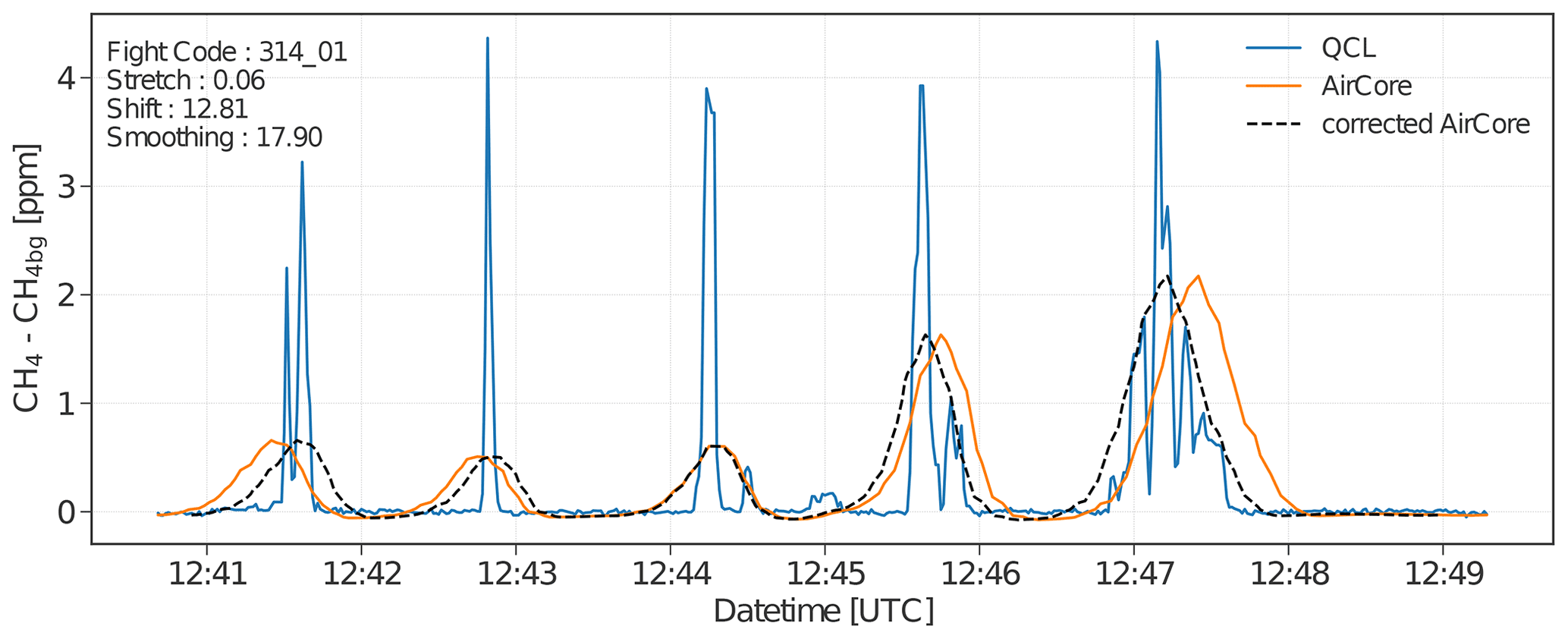
Figure 4 Methane mole fraction time series obtained by simultaneously flying the active AirCore system (orange line) and the in situ QCLAS analyser (blue line). The dashed black line represents the corrected AirCore measurements using the shifting and stretching parameters obtained from the 3S algorithm.

To determine the magnitude of smoothing present in the AirCore measurements, we flew the two instruments simultaneously with the UAV, while measuring the same point source downwind, as shown in Fig. 1. We then transformed the fast-response QCLAS measurements to mimic the smooth and smeared out AirCore data for each quantification flight where both instruments were present. Using the in-flight spectral calibration algorithm of imaging spectrometers developed by Kuhlmann et al. (2016), we obtained the smoothing, shifting, and stretching (3S) parameters needed in transforming the QCLAS measurements to match the measurements from the AirCore.

The smoothing of the AirCore measurements is dominated by the response of the CRDS analyser, i.e. air mixing in the analyser cavity (Andersen et al., 2022; Vinkovic et al., 2022), but is also influenced by molecular diffusion during sample storage as well as Taylor diffusion during sampling and analysis (Karion et al., 2010). We approximate the active AirCore measurement as y, defined as

$$\begin{array}{}\text{(5)}& y=f(x,b)+e,\end{array}$$

where f is a model function that fits the high-resolution QCLAS and projects it onto the low-resolution AirCore measurement. The model function consists of x, which is the independent variable where the QCLAS is measured (i.e. timescale), and the fit parameters b containing three elements describing the shift, stretch, and smoothing (i.e. 3S) of the AirCore. The error e represents the instrument's error as well as the error from the model function. We used a first-order Lagrange polynomial interpolation and applied a Gaussian filter with an initial width (1σ) of 10 s to parametrize the shift, stretch, and smoothing of the AirCore. Starting with an arbitrary initial guess, the optimal parameter $\widehat{b}$ was determined using a non-linear least-squares fit solved iteratively using the Gauss–Newton method.

4.5 Cluster-based kriging

In order to compute the flux through the vertical cross-section, the spatially discrete samples were interpolated to fill all gaps in the plane. Kriging is a popular method of stochastic interpolation in which the produced interpolated surface is modelled by a Gaussian process governed by prior covariance kernels, which is a realization of many possible outcomes that could have produced the known data points.

Kriging models have been widely used in atmospheric science and air quality as a tool for data analysis and prediction (e.g. Wong et al., 2004; Tadić et al., 2015, 2017; Michael et al., 2019). However, applying kriging to airborne measurements is faced with several challenges. Standard ordinary kriging assumes spatial stationarity of the geophysical field (Tadić et al., 2015), and all data points are assumed to be taken from a unimodal single probability distribution. Both assumptions are not necessarily true when a temporally varying plume is sampled sequentially over the duration of a flight. Furthermore, the scales of spatial variability of methane inside the plume and in the background are largely different, which violates the assumption of a unimodal distribution.

In order to overcome these issues, a cluster-based kriging (van Stein et al., 2020) was adapted. The process may be summarized into three main steps: (i) partitioning the dataset into smaller clusters, (ii) training an adequate kriging model for each cluster, and (iii) combining all kriging models to predict values (i.e. methane mole fractions) at unknown locations.

4.5.1 Data clustering

Cluster analysis or clustering is a process of grouping data into subsets according to a degree of similarity found inherently within the data. Clustering can be performed in many ways and can generally be divided into two basic types, hard and soft clustering.

Hard clustering is achieved when the data are split into smaller disjoint datasets, and the resulting label of a data point belongs to one and only one cluster. The most common example of an algorithm that implements hard clustering is k-means clustering. On the other hand, soft clustering splits the data into smaller datasets with small overlaps and returns a probability of how much a data point is associated with a specific cluster. A soft clustering approach is favoured in this study as this approach increases the final model accuracy (van Stein et al., 2020). One of the widely used models to perform soft clustering is a Gaussian mixture model (GMM) (Reynolds, 2015). A GMM is the type of model that will be used here.

Given a set $\mathcal{X}=\left\{({\mathit{x}}^{\mathrm{1}},y^{\mathrm{1}}),\mathrm{\dots },({\mathit{x}}^n,y^n)\right\}$ of methane mole fractions yⁱ acquired at locations xⁱ for $i=\left\{\mathrm{1},\mathrm{\dots },n\right\}$, where n is the number of data points collected, the goal is to split the input data 𝒳 into a set 𝒮, composed of several Gaussian components k, such that

$$\begin{array}{}\text{(6)}& \mathcal{S}=\mathit{\{}{\mathcal{X}}_{\mathrm{1}},\mathrm{\dots },{\mathcal{X}}_k\mathit{\}},\text{where}\bigcup _{j=\mathrm{1}}^k{\mathcal{X}}_j=\mathcal{X}.\end{array}$$

Each cluster 𝒳_j in the set 𝒮 is assumed to have a Gaussian shape in three dimensions, namely the 2D spatial location x and methane mole fraction y. The shape of each 𝒳_j being determined by a set of parameters ${\mathit{\theta }}_j=\left\{{\mathit{\pi }}_j,{\mathit{\mu }}_j,{\mathrm{\Sigma }}_j\right\}$, where π_j is the mixing probability, μ_j is the mean, and Σ_j is the covariance (i.e. spread) of the Gaussian. Each cluster 𝒳_j is acting together to model the overall density of 𝒳. The probability distribution of 𝒳 given a global mixture model parameter $\mathit{\theta }=\mathit{\{}{\mathit{\theta }}_{\mathrm{1}},\mathrm{\dots },{\mathit{\theta }}_k\mathit{\}}$ is defined as

$$\begin{array}{}\text{(7)}& p(\mathcal{X}\mid \mathit{\theta })=\sum _{j=\mathrm{1}}^k{\mathit{\pi }}_j\mathcal{N}({\mathcal{X}}_j\mid {\mathit{\mu }}_j,{\mathrm{\Sigma }}_j),\text{where}\sum _{j=\mathrm{1}}^k{\mathit{\pi }}_j=\mathrm{1},\end{array}$$

where 𝒩 is the normal distribution with mean μ_j and width Σ_j. The global mixture model parameter θ that best describes the data must be learned. The most established method to learn this parameter is through the use of an expectation–maximization (EM) algorithm. Given an initial parameter θ, the EM algorithm aims to estimate a new $\stackrel{\mathrm{‾}}{\mathit{\theta }}$, such that $p(\mathcal{X}\mid \stackrel{\mathrm{‾}}{\mathit{\theta }})\ge p(\mathcal{X}\mid \mathit{\theta })$. The new parameter then becomes the old parameter for the next iteration, and this process is repeated until a convergence threshold is satisfied. The a posteriori probability of a data point (xⁱ,yⁱ) belonging to cluster 𝒳_j with parameters θ_j is then given by

$$\begin{array}{}\text{(8)}& \begin{array}{rl}& \text{Pr}\left(\right({\mathit{x}}^i,y^i)\in {\mathcal{X}}_j\mid {\mathit{\theta }}_j)={\displaystyle \frac{{\mathit{\pi }}_j\mathcal{N}({\mathcal{X}}_j\mid {\mathit{\mu }}_j,{\mathrm{\Sigma }}_j)}{{\sum }_{j=\mathrm{1}}^k{\mathit{\pi }}_j\mathcal{N}({\mathcal{X}}_j\mid {\mathit{\mu }}_j,{\mathrm{\Sigma }}_j)}}\\ & \text{for}j=\mathrm{1},\mathrm{\dots },k.\end{array}\end{array}$$

Once the model parameter θ and the membership probability of a data point belonging to a cluster is learned, the clustered data points are expanded to the whole domain, and the membership probability of an unobserved location point ${\mathit{x}}_j^t$ belonging to cluster 𝒳_j is computed as well.

For typical trace gas distribution modelling, Stachniss et al. (2009) suggested the use of a mixture of only two clusters. The first cluster corresponds to measured background mole fractions, whereas the second cluster corresponds to elevated measurements. This choice is motivated by the fact that the spatial scales of variability are largely different between the two clusters. Tests with larger mixtures applied to our dataset showed that a two-cluster mixture is indeed sufficient to achieve good results.

4.5.2 Kriging estimate

Once the dataset has been clustered and the membership probability of each data point belonging to a cluster has been computed, ordinary kriging models are trained for each cluster separately to spatially interpolate the field of interest. Since data points for ordinary kriging can only belong to one of the two clusters, the kriging model for each cluster is learned using hard clustered data points, either belonging to the background or the elevated cluster. Hard clustered data points are obtained by rounding the probability obtained from the GMM to either belong to the background or the elevated cluster. Interpolation of a geophysical field from a spatially sparse dataset is highly dependent on a chosen covariance kernel K, which statistically describes the relationship between two spatial points using a set of hyper-parameters $\mathit{\lambda }=\left\{l,\mathit{\sigma }\right\}$, where l refers to the length-scale, and σ² is the overall variance (i.e. noise) coming from the data. There are several ways to define the covariance kernel. In this study, the Matèrn 5/2 covariance kernel is chosen as it performs better compared to other frequently used kernels, such as a squared exponential function as shown by Stachniss et al. (2009). In their study, they established that the Matèrn covariance kernel has a lesser degree of smoothing compared to other kernels, which resembles more closely the nature of gas distributions in the vicinity of a localized source. Optimizing the hyper-parameters of the covariance kernel K for each cluster is done by evaluating a log-marginal-likelihood (LML) using a set of initial parameters, which are increased or decreased incrementally until a maximum value is obtained. The whole process of clustering the dataset into two clusters followed by optimizing the hyper-parameters of each cluster was implemented using the scikit-learn package of Python.

Optimized hyper-parameters ${\mathit{\lambda }}_j=\mathit{\{}{l}_j,{\mathit{\sigma }}_j\mathit{\}}$ for each cluster 𝒳_j are used to perform ordinary kriging to predict a data point $({\mathit{x}}_j^t,y_j^t)$ of unmeasured methane mole fraction $y_j^t$ at an unobserved location ${\mathit{x}}_j^t$. The resulting interpolated field from kriging is a Gaussian distribution 𝒩 expressed as

$$\begin{array}{}\text{(9)}& y_j^t\mid {\mathcal{X}}_j\sim \mathcal{N}\left(m_j\left({\mathit{x}}^t\right),s_j^{\mathrm{2}}\left({\mathit{x}}^t\right)\right),\end{array}$$

with mean m_j and variance $s_j^{\mathrm{2}}$.

The final predicted value (x^t,y^t) of methane mole fractions y^t at each point (x^t,y^t) is obtained by combining the results of all the kriging models together $({\mathit{x}}_j^t,y_j^t)$ with the respective membership probability of each spatial point x^t used as weights w_j, denoted as

$$\begin{array}{}\text{(10)}& w_j=\text{Pr}\left(C=j\mid \mathcal{X},{\mathit{x}}^t\right),\text{for}j=\mathrm{1},\mathrm{\dots },k,\end{array}$$

where C is the cluster indicator ranging from 1 to k.

Thus, the expected value of methane mole fraction y^t at each spatial point x^t is

$$\begin{array}{}\text{(11)}& \mathbf{E}\left[y^t\mid \mathcal{X},y,{\mathit{x}}^t\right]=\sum _{j=\mathrm{1}}^k{w}_j{m}_j\left({\mathit{x}}^t\right),\end{array}$$

and the variance of the expected value is (van Stein et al., 2020)

$$\begin{array}{}\text{(12)}& \begin{array}{rl}\text{Var}\left[y^t\mid \mathcal{X},y,x^t\right]=& \sum _{j=\mathrm{1}}^k{w}_j(s_j^{\mathrm{2}}\left({\mathit{x}}^t\right)+m_j^{\mathrm{2}}\left({\mathit{x}}^t\right))\\ & -{\left(\sum _{j=\mathrm{1}}^k{w}_j{m}_j\left({\mathit{x}}^t\right)\right)}^{\mathrm{2}}.\end{array}\end{array}$$

Although other kriging option modules are available such as a moving neighbourhood approach where only data points within a certain radius are considered in the kriging process (Mays et al., 2009; O'Shea et al., 2014; Pitt et al., 2019), the cluster-based kriging approach offers the advantage of removing many arbitrary subjective parameters present in other approaches.

4.6 Example of quantification procedure

An illustration of the clustering and kriging approach used to map a discrete set of data points onto the whole measurement plane is presented in Figs. 5 and 6 for flight 312_03 on 12 March 2020. The time series presented in the upper left panel of Fig. 5 was first mapped onto the 2D measurement plane composed of horizontal distance and vertical altitude. The time series, composed of a set of ordered spatial and methane concentration points (x,y), was then fed into a GMM to partition the dataset into two clusters, namely, the background and the elevated cluster. The GMM returns the membership probability of a data point belonging to one cluster or the other. The membership probability of each data point was then expanded to the whole domain to unobserved locations as shown in Fig. 6a. In a next step, ordinary kriging was applied to each cluster separately to produce a background and an elevated CH₄ distribution (Fig. 6a left panels). Finally, the kriging results for each cluster were combined with their respective membership probability. The resulting kriging field is illustrated in Fig. 6b, with the expected value computed according to Eq. (11) and prediction uncertainty, i.e. the square root of variance according to Eq. (12). A reconstructed time series of predicted methane mole fraction was compared to the original time series of measured methane and is shown in Fig. S1 in the Supplement. The peaks of predicted methane mole fraction are lower but broader compared to the original methane time series as expected as kriging applies smoothing in the data.

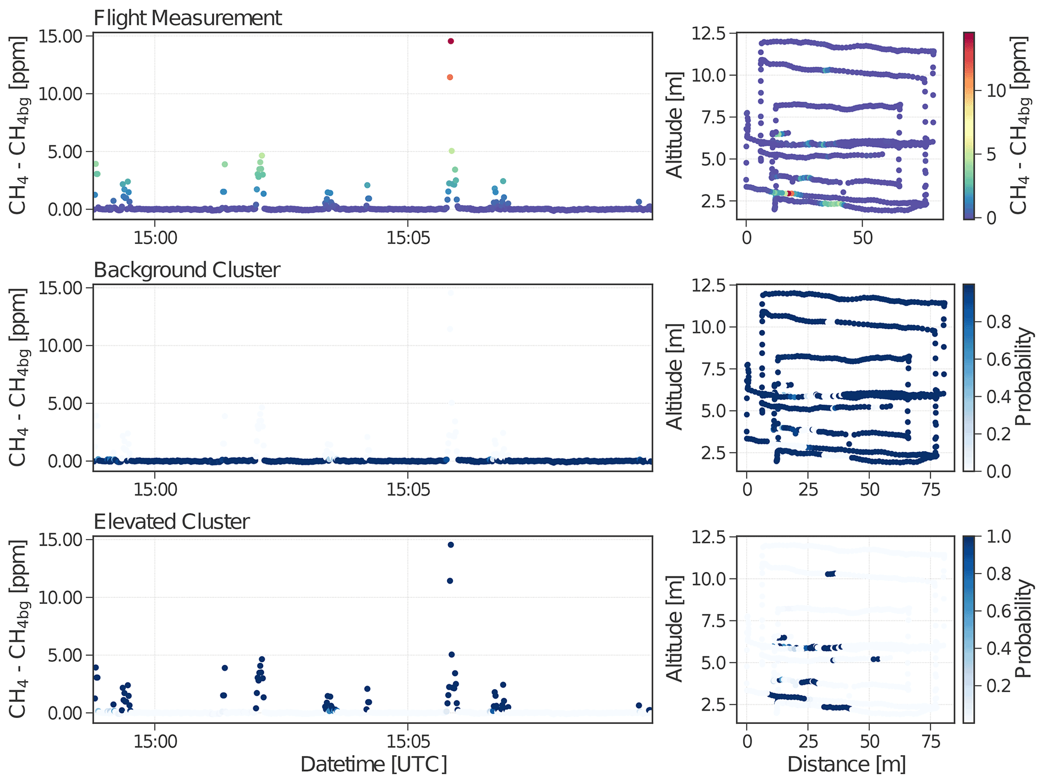
Figure 5 Clustering result for flight 312_03 on 12 March 2020 obtained from the in situ QCLAS after applying a GMM with two mixture components. The background and elevated cluster complement each other; the total probability of each data point shared between the two clusters is equal to 1a.

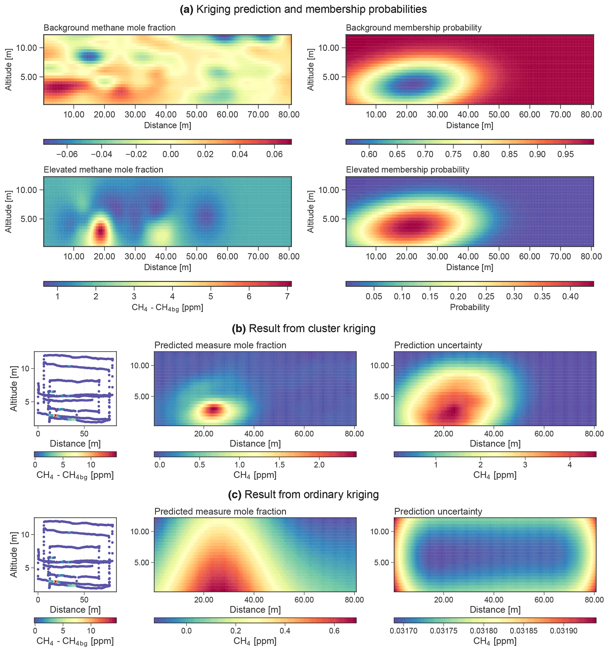
Figure 6 (a) Kriging prediction and membership probabilities of each spatial point within the domain of interest for background and elevated clusters. (b) Expected value and variance of methane mole fractions after combining kriging prediction of the two clusters and their respective membership probabilities. (c) Expected value and variance of methane mole fractions using ordinary kriging.

The measured average ambient air temperature T [K] and pressure p [Pa] during the flight was used to convert the obtained kriging field of methane mole fraction ${\mathit{\chi }}_{{\mathrm{CH}}_{\mathrm{4}}}$ [ppm] into concentrations ${\mathit{\rho }}_{{\mathrm{CH}}_{\mathrm{4}}}$ [g m⁻³]:

$$\begin{array}{}\text{(13)}& {\mathit{\rho }}_{{\mathrm{CH}}_{\mathrm{4}}}={\mathit{\chi }}_{{\mathrm{CH}}_{\mathrm{4}}}{\displaystyle \frac{p{M}_{{\mathrm{CH}}_{\mathrm{4}}}}{RT}},\end{array}$$

where R is the gas constant (8.3144 J K⁻¹ mol⁻¹), and $M_{{\mathrm{CH}}_{\mathrm{4}}}$ is the molar mass of methane (16.04 g mol⁻¹). The influence of humidity, which introduces an error of no more than 1 %, was ignored in this equation. As we are only interested in methane elevations above the background, this uncertainty is considered small.

The concentration field was combined with wind fields using three different wind treatments as discussed in Sect. 4. Finally, an emission rate Q_c was estimated as a scalar (dot) product of the concentration field C and the wind field U written as vectors:

$$\begin{array}{}\text{(14)}& Q_{\mathrm{c}}=\left({\mathit{C}}^{\top }\cdot \mathit{U}\right)\mathrm{\Delta }y\mathrm{\Delta }z,\end{array}$$

where Δy and Δz are the regularly spaced intervals in the horizontal and vertical direction.

The emission rate Q_c(C,U) is a function of two variables C and U, and the overall error propagation of the function is

$$\begin{array}{}\text{(15)}& \mathrm{\Delta }{Q}_{\mathrm{c}}^{\mathrm{2}}={\left({\displaystyle \frac{\partial Q_{\mathrm{c}}}{\partial \mathit{C}}}\mathrm{\Delta }\mathit{U}\right)}^{\mathrm{2}}+{\left({\displaystyle \frac{\partial Q_{\mathrm{c}}}{\partial \mathit{U}}}\mathrm{\Delta }\mathit{C}\right)}^{\mathrm{2}}\mathrm{\Delta }{y}^{\mathrm{2}}\mathrm{\Delta }{z}^{\mathrm{2}}.\end{array}$$

The concentration field C and wind field U come with their respective covariance matrix K_C and K_U provided by kriging, and the above equation becomes

$$\begin{array}{}\text{(16)}& \mathrm{\Delta }{Q}_{\mathrm{c}}^{\mathrm{2}}=\left({\mathit{U}}^{\top }\cdot {\mathbf{K}}_{\mathrm{C}}\cdot \mathit{U}+{\mathit{C}}^{\top }\cdot {\mathbf{K}}_{\mathrm{U}}\cdot \mathit{C}\right)\mathrm{\Delta }{y}^{\mathrm{2}}\mathrm{\Delta }{z}^{\mathrm{2}}.\end{array}$$

In cases where U is a scalar constant or logarithmic profile, the uncertainty of the wind is estimated by computing the standard deviation (1σ) of the mean wind speed normal to the measurement plane during the flight.

Cluster-based kriging produces the concentration field C as a linear combination of two distinct concentration fields C_elev and C_bg with weights w_elev and w_bg:

$$\begin{array}{}\text{(17)}& \mathit{C}={\mathit{w}}_{\mathrm{elev}}{\mathit{C}}_{\mathrm{elev}}+{\mathit{w}}_{\mathrm{bg}}{\mathit{C}}_{\mathrm{bg}},\end{array}$$

where w_elev and w_bg are vectors of the same length as C_elev and C_bg. Both concentration fields come with a covariance matrix K_Celev and K_Cbg as determined by kriging. The weights w_elev and w_bg are constants without uncertainties.

The concentration field C(C_elev,C_bg) is a function of two variables C_elev and C_bg, and the error propagation of the function is

$$\begin{array}{}\text{(18)}& \mathrm{\Delta }{\mathit{C}}^{\mathrm{2}}={\left({\displaystyle \frac{\partial C}{\partial {\mathit{C}}_{\mathrm{elev}}}}\mathrm{\Delta }{\mathit{C}}_{\mathrm{elev}}\right)}^{\mathrm{2}}+{\left({\displaystyle \frac{\partial C}{\partial {\mathit{C}}_{\mathrm{bg}}}}\mathrm{\Delta }{\mathit{C}}_{\mathrm{bg}}\right)}^{\mathrm{2}},\end{array}$$

written in matrix notation as

$$\begin{array}{}\text{(19)}& {\mathbf{K}}_{\mathrm{C}}=\mathrm{\Delta }{\mathit{C}}^{\mathrm{2}}={\mathit{w}}_{\mathrm{elev}}\cdot {\mathit{w}}_{\mathrm{elev}}^{\top }\cdot {\mathbf{K}}_{\mathrm{Celev}}+{\mathit{w}}_{\mathrm{bg}}\cdot {\mathit{w}}_{\mathrm{bg}}^{\top }\cdot {\mathbf{K}}_{\mathrm{Cbg}}.\end{array}$$

5 Results and discussion

5.1 Emission estimates

Measurements from 18 flights were analysed to characterize the accuracy of the quantification method. A total of six quantification approaches were applied to all flights and evaluated for their ability to reproduce the true releases. These approaches arise from the combination of two different treatments of methane measurements and three different treatments of wind measurements. The treatments involved in mapping the discrete methane points into the measurement plane are the standard ordinary kriging (OK) and the cluster-based kriging (CK) interpolation schemes. The three different ways of estimating wind speeds during each quantification flight involve the scalar wind (SW), logarithmic wind (LW), and projected wind (PW), as discussed in Sect. 4.

The overall performance of each quantification approach is presented in Table 2 and estimated emission rates together with the true release rates for every individual flight are presented in Table S1 in the Supplement. Estimates are presented for six different quantification methods, which correspond to three different wind treatments applied to two different kriging methods, standard ordinary kriging and cluster kriging, as described above. Among all the methods, the best-performing approach, characterized by the lowest RMSE, was obtained by applying cluster kriging with projected wind (CKPW), where methane measurements were clustered before kriging and where the normal components of the instantaneous wind measurements were projected onto the positions of the UAV.

Table 2 Summary of performance of each quantification approach.

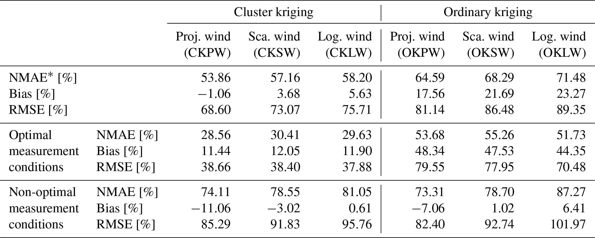
^* Normalized mean absolute error. Optimal and non-optimal measurement conditions are defined in Sect. 5.1.2.

A residual plot showing the accuracy of each quantification approach relative to the true release is presented in Fig. 7. The plot illustrates the amount by which we underestimated (negative numbers) or overestimated (positive numbers) the known release for each measurement flight.

Figure 7 Residual plot. Colour-coded solid bars represent the range of residuals using different quantification approaches, with the mean values represented as black dots. Values to the right of the red line correspond to overestimations, and values to the left correspond to underestimations. CK and OK stand for cluster kriging and ordinary kriging, respectively. PW (projected wind), SW (scalar wind), and LW (logarithmic wind) refer to the different wind data treatments.

In general, a good agreement between computed estimates using the CKPW approach and true releases was observed as the uncertainty range managed to capture the known release for most measurement flights. A slight overestimation was observed for most of the earlier flights, but release rates were captured well within the uncertainty range provided by the CKPW approach. We have observed a systemic underestimation for the last six flights on 13 and 14 March, where we did not manage to capture the true release for four flights (i.e. 313_03, 313_04, 314_01, and 314_02). In order to investigate the reasons for this underestimation, we compared the predicted kriging fields with a theoretical Gaussian plume dispersion model (see Figs. S2 and S3) to test whether the vertical and horizontal distance flown by the UAV was sufficient to capture the whole plume. The Gaussian plume model using a Pasquill–Gifford stability class dispersion parameterization scheme provides an analytical solution for the horizontal and vertical width as a function of downwind distance depending on wind speed and atmospheric stability. The comparison with the size of the theoretical Gaussian plume suggests that although we managed to detect methane elevations, we were most likely not able to capture the whole extent of the plume during these flights. The reason is that some of these flights were conducted at a rather large distance from the source and under low wind conditions, during which the plume spreads more quickly with downwind distance. For flights 313_03–05, for example, the horizontal and vertical width of the Gaussian plume computed for the meteorological conditions and downwind distance of the flight was on average 75 and 20 m, respectively. However, the typical cross-sectional plane covered by the UAV was of the order of 100 m×12 m, which is insufficient to fully capture a spread of the calculated plume, especially with respect to the vertical extent.

The average horizontal and vertical spread of the plume with respect to wind speed and downwind distance computed with the Gaussian plume model is illustrated in Fig. 8. The spread does not vary smoothly with wind speed but shows step-wise changes because the model uses different (but fixed) dispersion parameters for different wind speed and stability classes. Overlaid on top are dots coloured from white to red representing the performance of each measurement flight with lighter colours showing smaller relative errors. It can be seen that flights with the highest accuracy are the ones that fall within the blueish region characterized by wind speeds greater than 2 m s⁻¹ and a sampling downwind distance ranging from 10 to 75 m. Measurement flights within this region had a higher accuracy mainly because the vertical spread of the plume was below 10 m, which is a realistic range for the UAV to completely map the plume. For optimal measurement conditions, we found a slight positive bias of 11 % using the CKPW method and an RMSE of 39 %. Measurements under suboptimal conditions had a smaller average bias (about −11 %) but a much larger spread with a significant overestimation and underestimation with an RMSE of 85 %.

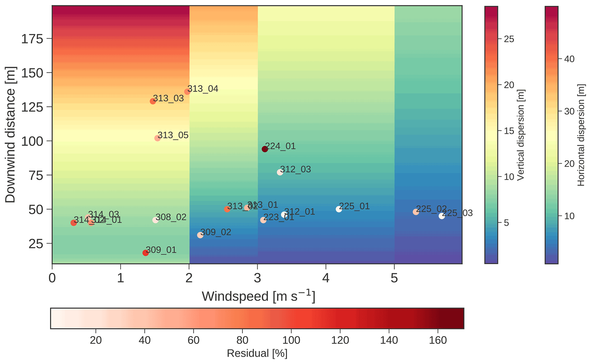
Figure 8 Theoretical horizontal and vertical spread of a plume with respect to wind speed and downwind distance. White to red dots refers to the individual error of each quantification flight, lighter being more accurate than darker dots.

All measurement flights were also analysed using an ordinary kriging (OK) algorithm, where methane measurements were not clustered before kriging. By doing so, each measurement flight was fed directly into a GMM to determine the hyper-parameters for kriging. Likewise, the Matèrn 5/2 covariance kernel was used to quantify the correlation between the measured data. Ordinary kriging produces a single methane field with expected value and variance because a single correlation length scale is assumed for both the background and the plume data. The assumption of a single correlation length leads to a strong smoothing of the plume (Stachniss et al., 2009), as illustrated in Fig. 6c. Obtained methane fields were combined with the same three different wind treatments to compute the release rates. A summary of emission rates computed using ordinary kriging is presented in Table 2, and the range of the residuals for each quantification approach is illustrated in Fig. 9. It shows that cluster-based kriging, in general, outperforms ordinary kriging, as evidenced by lower RMSE and lower relative absolute errors. On average, all data treatments tend to overestimate the true release, but the lowest overestimation was obtained using the CKPW approach. Generally, a larger variability of residuals (wider interquartile band) was obtained for the approaches using OK as compared to the respective CK counterpart. A concrete example to see the difference between the reconstructed methane plume using cluster kriging and ordinary kriging is presented for flight 312_03 in Fig. 6b and c. CK proves to better preserve the shape of the plumes, which results in a better accuracy of the estimates.

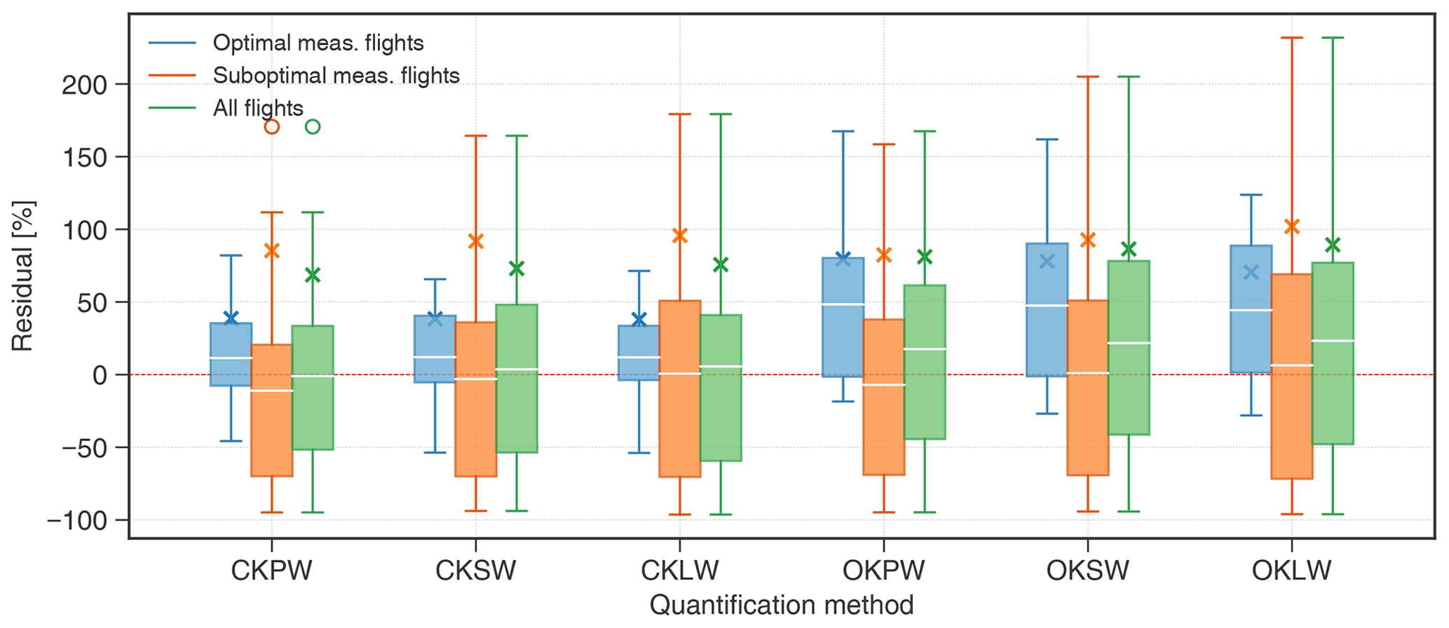
Figure 9 Colour-coded box plots represent the range of residuals in flux estimates of measurement flights grouped according to meteorological and threshold conditions. Solid white lines represent the mean bias and the × marks represent the RMSE for each quantification approach. Definitions of optimal and suboptimal measurement flights are defined in Sect. 5.1.2.

5.1.1 Impact of altitude uncertainties on emission estimates

Initially, the altitude measurements of the UAV-based system were relying exclusively on the onboard internal GPS, but later it became evident that this has some impact on our capability of emission estimates. The RTK-GPS system was implemented a few days after the start of the MATRIX campaign, and 11 out of 18 measurement flights contain both UAV altitude and RTK altitude. We observed an average drift of the UAV-GPS of 0.10 cm s⁻¹, which translates to an altitude error of about 0.6 m for a 10 min flight duration. This drift is consistent with the uncertainty reported by the UAV manufacturer, though sometimes errors were larger, up to 0.20 cm s⁻¹ (see Table S2). An erroneous altitude retrieval on certain flight levels may lead to a distortion of the emission plume, which ultimately affects the estimated emissions (see Fig. S4). A summary of the percentage difference between the emission estimates derived using two different altitudes is presented in Fig. 10. Differences are in the range of −8 % to 18 %, with an absolute average difference of 4 %, suggesting that the errors introduced by inaccurate vertical positioning are relatively small compared to the overall uncertainty of the CKPW quantification method. The highest differences occurred on flights 313_02 and 313_05, during which the drift of the UAV-GPS was particularly large (about 0.17 cm s⁻¹; see Table S2). These findings are also important aspects in the context of the ROMEO campaign, during which the high-accuracy RTK-GPS system was not yet implemented. Now, it can be stated that the emissions reported for the ROMEO campaign should have a similar accuracy as presented here, at least for those cases where meteorological conditions were favourable.

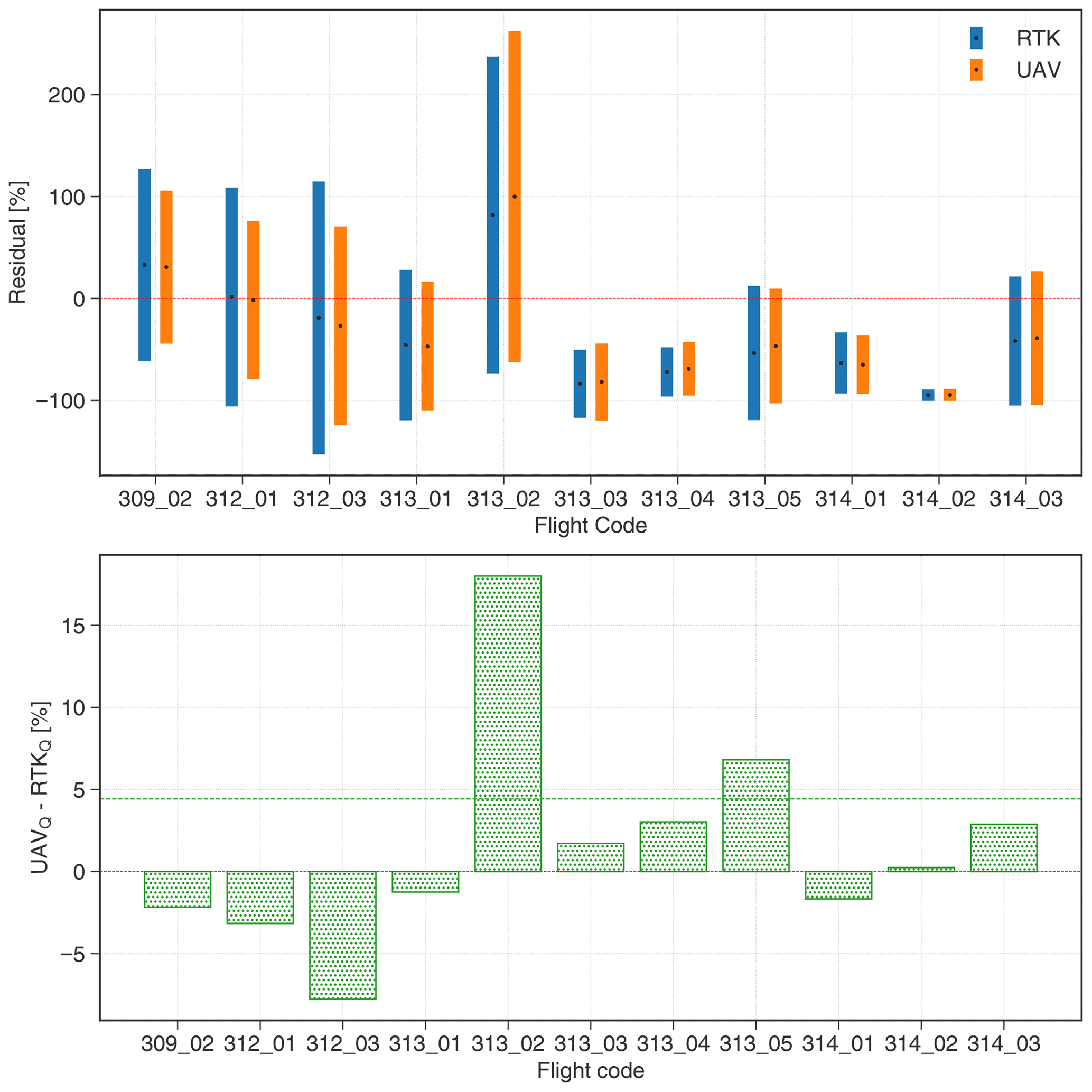
Figure 10 Difference in emission estimates using two different GPS altitudes. The dashed green line represents the absolute average difference between the two estimates.

5.1.2 Impact of wind speed and direction on emission estimates

Similar to our study, Yang et al. (2018) performed a rasterized mass-balance approach to quantify emissions from individual gas wells in Texas, United States, using UAVs. Based on their results, they proposed a minimum threshold of wind speed of 2.3 m s⁻¹ and wind direction variability not greater than 33.1^∘ in order to quantify emissions with an accuracy of better than 50 %. Applying the same threshold criteria and additionally restricting the measurements to a maximum downwind distance of 75 m, we have identified 8 out of 18 flights from our campaign that satisfy these criteria (see Fig. S5). As illustrated in Fig. 9, these flights indeed exhibit a lower RMSE and absolute mean error. RMSE and absolute error were reduced to 39 % and 29 % respectively as compared to 69 % RMSE and 54 % absolute error for all flights. Computed emission rates were on average slightly overestimated by 11 %. In contrast, a lower average accuracy was observed when measurement flights were performed under less favourable wind conditions. Computed emission rates under these conditions were generally underestimated by 11 %, with a higher corresponding RMSE and absolute mean error of 85 % and 74 %. Underestimation of true releases during highly variable weather conditions may be attributed to incomplete sampling of methane plumes, as discussed above. Variability of residuals (width of interquartile band) among all approaches is significantly lower for measurement flights under optimal conditions as compared to measurements performed in suboptimal conditions.

5.2 Comparison of AirCore and QCLAS emission estimates

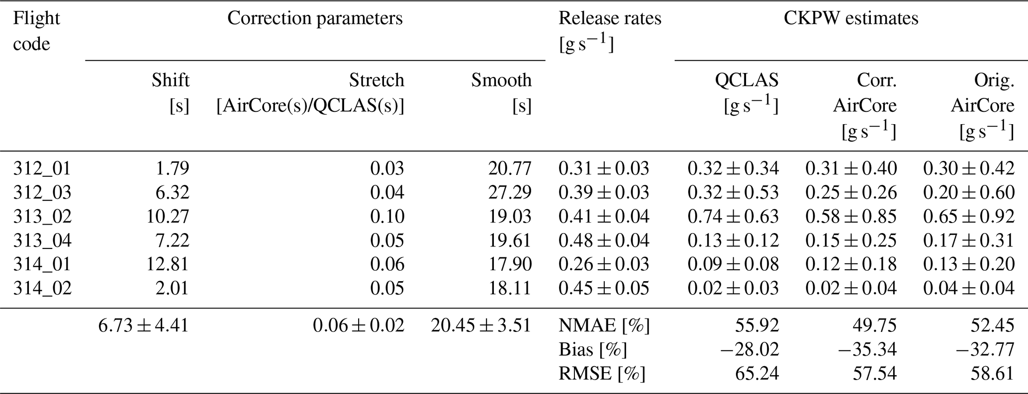
Having simultaneous samples of methane plumes using the QCLAS and AirCore systems, we have found that the AirCore measurements were smoothed by an average of 20 s (1σ) using a Gaussian smoothing function when compared with measurements using the QCLAS. We also observed that AirCore measurements are temporally shifted by an average of 7 s and are stretched linearly with time at an average rate of 0.06 s for every second of QCLAS measurement. The smoothing, stretching, and shifting parameters obtained for each individual flight are presented in Table 3. Corrected and original AirCore methane measurement flights were subject to the CKPW quantification approach to compare how the stretched and shifted AirCore measurements affect the quantifications. Emissions are compared to emission estimates using QCLAS measurements to see the degree of agreement between the two systems. A summary comparing the differences in emission estimates is presented in Table 3. We have observed that the emission estimate computed using the corrected time series is 3 % more accurate compared to its original counterpart. Nevertheless, the uncertainty bounds of most quantification flights manage to capture the true release. In extreme cases, where the time shift and stretching are not sufficiently well known, the size and location of the plume might not be captured accurately. As an example, a comparison of reconstructed plume with and without applying proper correction for flight 312_03 is illustrated in Fig. S6. The figure shows that the uncorrected reconstructed plume tends to be cut on the left side of the mapping plane. After applying the proper correction, the plume shifted to the right, putting the methane plume closer to the centre of the mapping plane. This resulted in a 23 % increase in the emission estimate, bringing it much closer to the actual release. Thus, even though uncertainty bounds manage to capture most of the releases, accounting for the proper time shift and stretching of the AirCore data is important when performing a mass-balance quantification approach, especially in extreme cases.

Table 3 Correction parameters and calculated emission rates for AirCore measurements.

5.3 Comparison with other methodologies

A direct comparison with another method was performed for the OTM-33A method. Quantified releases using OTM-33A and our mass-balance approach are summarized in Table 4. Although the number of simultaneous quantifications is limited, the results show that both approaches are close to the true release and that the uncertainty bounds of both methods usually capture the true release. This showcases that our UAV-based quantification technique has a great potential and is on a par with measuring CH₄ emissions from oil and gas wells when compared with the OTM-33A method. Emission estimates using OTM-33A for flight 225_01–03 were identical because OTM-33A estimates are more robust if the input data last longer than 20 min. Since the release rate during that day was constant and continuous, one emission estimate was used for the three UAV-flight emission estimates for that day.

Table 4 Emission rates from QCL-CKPW and OTM-33A in g s⁻¹.

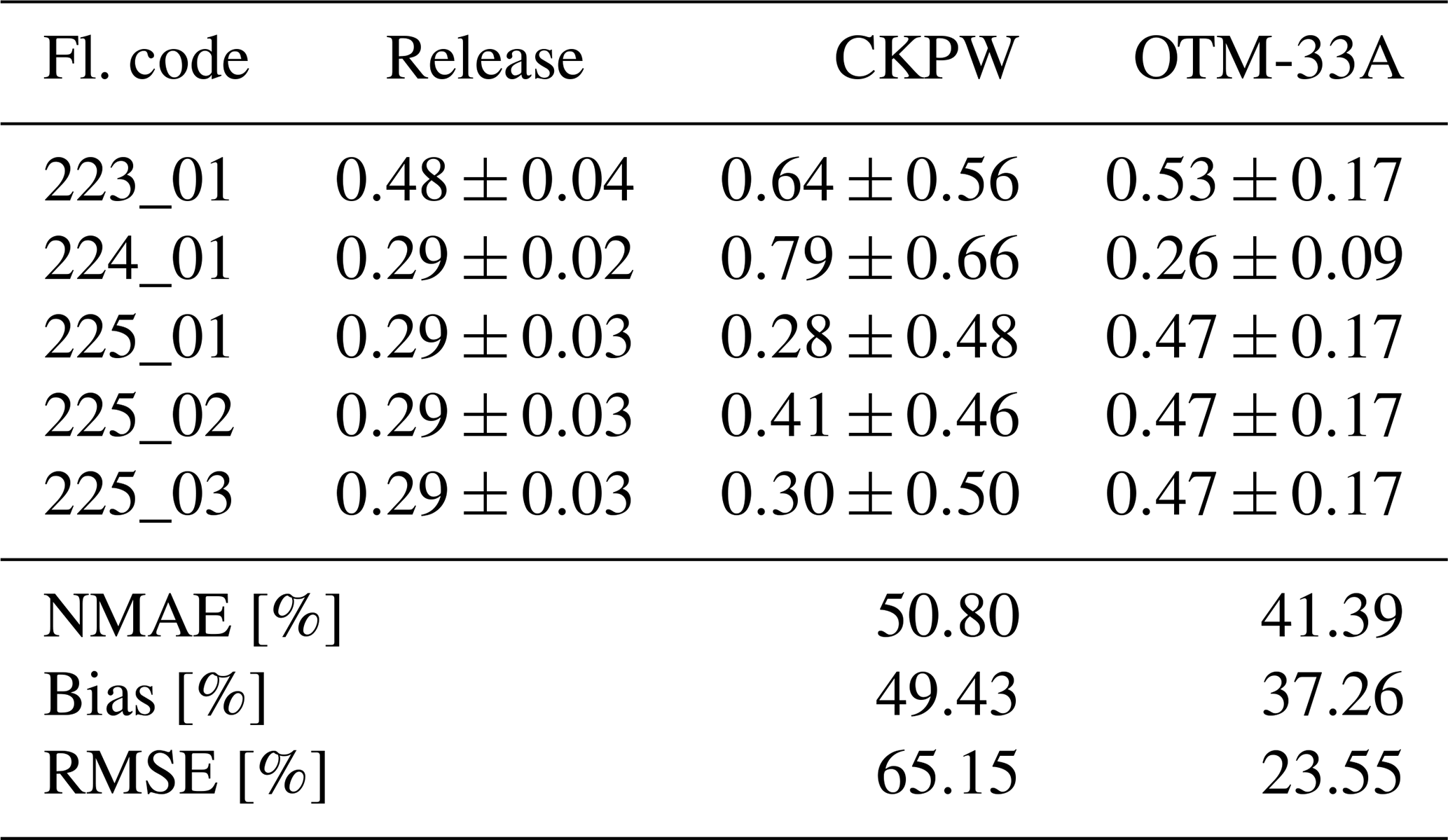
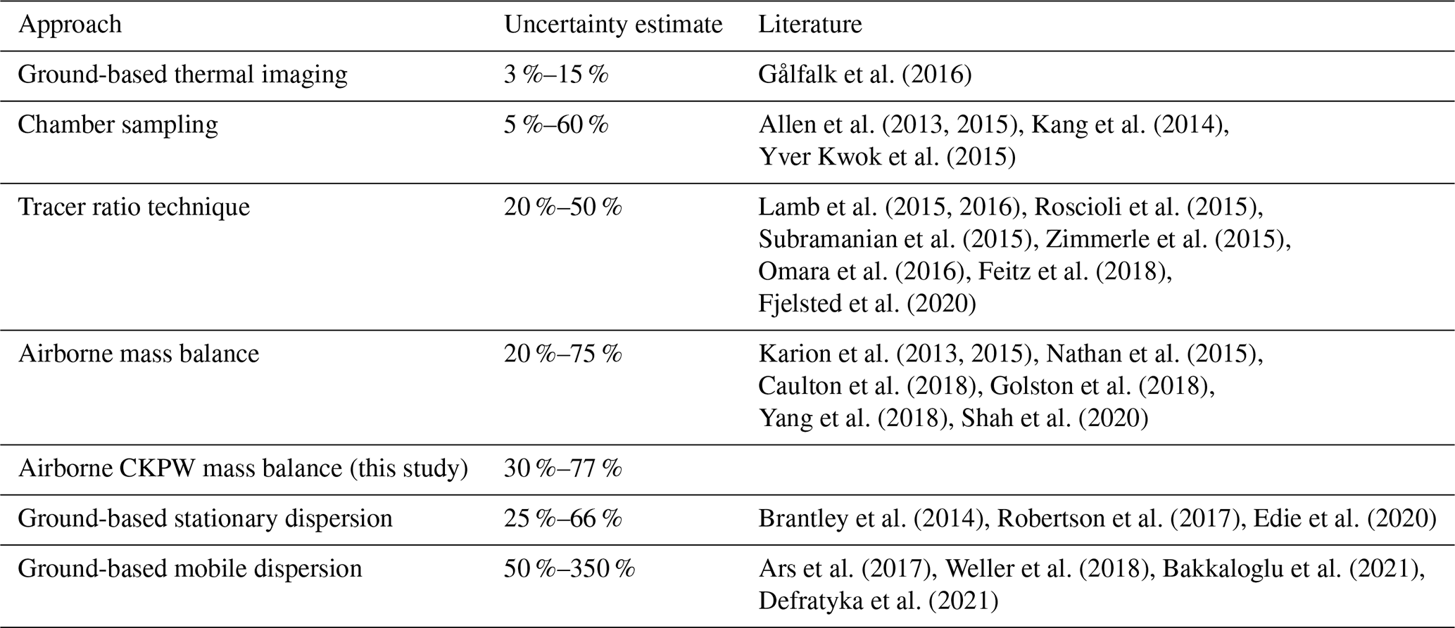
Table 5 compares the uncertainty of our UAV-based quantification method with other methods as previously summarized by Caulton et al. (2018). With an accuracy ranging from 28 % to 75 %, our method is on a par with existing quantification techniques, specifically with mass-balance approaches using aircraft/UAVs. A major advantage of our UAV-based method is that it can be applied to sources that are not easily accessible and where no road is present in a suitable distance perpendicular to wind direction for ground-based mobile measurements. Another advantage is that it can be applied to quantify the total emissions of a cluster of sources, provided that the UAV can map the full extent of all individual source plumes. Ideally, the emission from an individual source should be quantified multiple times. The individual estimates provide an invaluable measure of uncertainty in addition to the method uncertainty estimated here for individual flights. This is even more important under highly unstable and turbulent conditions, since an individual flight can only capture a snapshot of a turbulent plume.

Gålfalk et al. (2016)Allen et al. (2013, 2015)Kang et al. (2014)Yver Kwok et al. (2015)Lamb et al. (2015, 2016)Roscioli et al. (2015)Subramanian et al. (2015)Zimmerle et al. (2015)Omara et al. (2016)Feitz et al. (2018)Fjelsted et al. (2020)Karion et al. (2013, 2015)Nathan et al. (2015)Caulton et al. (2018)Golston et al. (2018)Yang et al. (2018)Shah et al. (2020)Brantley et al. (2014)Robertson et al. (2017)Edie et al. (2020)Ars et al. (2017)Weller et al. (2018)Bakkaloglu et al. (2021)Defratyka et al. (2021)

Table 5 Uncertainty of different CH₄ emission quantification techniques.

6 Conclusions

A novel strategy of methane flux quantification with the use of unmanned aerial vehicles (UAVs) equipped with a methane sensor has been developed and applied to an extensive controlled-release experiment. Real-time atmospheric methane mole fractions were measured in situ using a quantum cascade laser spectrometer (QCLAS) and an active AirCore system. Both instruments are lightweight and have a compact footprint, allowing them to be mounted on commercially available UAVs. Emissions were quantified by applying a cross-sectional mass-balance approach. An extensive controlled-release experiment was conducted in Dübendorf, Switzerland, from 23 February to 14 March 2020 to develop, optimize, and evaluate the method. In addition, source quantification from the UAV was compared for selected cases with results from stationary measurements applying the OTM-33A method.

The mass-balance approach was performed by flying the UAV-integrated system at a cross-section downwind of the source at multiple vertical levels. Methane mole fraction measurements were subject to two different data treatments, while the wind measurements were treated in three different ways, thus giving us in total six methane-quantification approaches. Each of these were applied to all flights and evaluated for their ability to reproduce the true releases.

During the campaign, 18 flights suitable for emission quantification could be performed. Among the six quantification approaches, the best results were obtained using the CKPW (cluster kriging with projected wind) approach. The true release could be estimated with a normalized mean absolute percentage error of 54 %. The highest absolute percentage error of 71 % was obtained using the OKLW (ordinary kriging with logarithmic wind profile) approach. A consistent underestimation of methane fluxes occurred in our quantification approach when the mass-balance method was performed at a downwind distance of more than 75 m. Simulations with a simple Gaussian plume model suggest that we were most likely not able to capture the whole extent of the plume during these flights, especially with respect to its vertical extent. Comparison of QCLAS-CKPW emission estimates with quantified emission rates using an independent ground-based quantification technique, OTM-33A, shows that both methods captured the true release almost every time.

As a general guideline, performing UAV-based emission quantification of emission sources requires favourable wind conditions with a minimum wind speed of 2.3 m s⁻¹ and a maximum wind direction variability of 33.1^∘. Under these conditions, measuring at a downwind distance of less than 75 m ensures the true emission to be fully mapped, both horizontally and vertically. In cases where an RTK-GPS is not present, a vertical spacing of at least 0.5 m is recommended to properly account for the average drift of a commercial UAV-GPS of about 0.11 cm s⁻¹.

Having a high-precision and fast CH₄ analyser, such as the QCLAS, offers the benefit of correctly mapping the methane plume both spatially and temporally as compared to other methods, such as collecting air samples with subsequent analysis on the ground. In extreme cases, poor mapping of the emission may ultimately lead to over- or underestimation of its value. This is evidenced in one of the measurement flights, i.e. 312_03, where a reconstructed methane plume using the uncorrected AirCore measurement resulted in a significant underestimation (about 48 %) of the true release. Nevertheless, the uncertainty bounds of the CKPW quantification approach usually manage to capture the true release.

In conclusion, UAV-based emission quantification using the CKPW approach proved its capability to quantify emission fluxes from methane point sources. This approach can be easily scaled up to confidently quantify total emissions for a cluster of sources given that the UAV system can map the full extent of all individual plumes. The use of UAVs in quantifying localized methane sources offers an advantage of allowing for additional freedom of sampling locations where stationary monitors and ground-based mobile sensors cannot be deployed. It also allows for rapid adjustment to changing wind conditions, which proved to be particularly beneficial during the ROMEO measurement campaign, where a large number of oil and gas wells had to be quantified in a short amount of time.