the Creative Commons Attribution 4.0 License.
the Creative Commons Attribution 4.0 License.
 | 14 Apr 2022
Retrieving H2O/HDO columns over cloudy and clear-sky scenes from the Tropospheric Monitoring Instrument (TROPOMI)
Andreas Schneider
Joost aan de Brugh
Alba Lorente
Franziska Aemisegger
David Noone
Dean Henze
Rigel Kivi
Jochen Landgraf
This paper presents an extended scientific HDO/H2O total column data product from short-wave infrared (SWIR) measurements by the Tropospheric Monitoring Instrument (TROPOMI) including clear-sky and cloudy scenes. The retrieval employs a forward model which accounts for scattering, and the algorithm infers the trace gas column information, surface properties, and effective cloud parameters from the observations. Compared to the previous clear-sky-only data product, coverage is greatly enhanced by including scenes over low clouds, particularly enabling data over oceans as the albedo of water in the SWIR spectral range is too low to retrieve under cloud-free conditions. The new dataset is validated against co-located ground-based Fourier transform infrared (FTIR) observations by the Total Carbon Column Observing Network (TCCON). The median bias for clear-sky scenes is 1.4×10²¹ molec cm−2 (2.9 %) in H2O columns and 1.1×10¹⁷ molec cm−2 (−0.3 %) in HDO columns, which corresponds to −17 ‰ (9.9 %) in a posteriori δD. The bias for cloudy scenes is 4.9×10²¹ molec cm−2 (11 %) in H2O, 1.1×10¹⁸ molec cm−2 (7.9 %) in HDO, and −20 ‰ (9.7 %) in a posteriori δD. At low-altitude stations, the bias is small at low and middle latitudes and has a larger value at high latitudes. At high-altitude stations, an altitude correction is required to compensate for different partial columns seen by the station and the satellite. The bias in a posteriori δD after altitude correction depends on sensitivity due to shielding by clouds and on realistic a priori profile shapes for both isotopologues. Cloudy scenes generally involve low sensitivity below the clouds, and since the information is filled up by the prior, a realistic shape of the prior is important for realistic total column estimation in these cases. Over oceans, aircraft measurements with the Water Isotope System for Precipitation and Entrainment Research (WISPER) instrument from a field campaign in 2018 are used for validation, yielding biases of −3.9 % in H2O and −3 ‰ in δD over clouds. To demonstrate the added value of the new dataset, a short case study of a cold air outbreak over the Atlantic Ocean in January 2020 is presented, showing the daily evolution of the event with single-overpass results.
- Article
(13824 KB) - Full-text XML
- BibTeX
- EndNote


Atmospheric moisture strongly controls Earth's radiative budget and transports energy via latent heat, e.g. from low to high latitudes. Uncertainties in the quantification of these two effects are still large and represent one of the key uncertainties in current climate prediction (Stevens and Bony, 2013). Isotopologues of water offer further insights into the water cycle due to fractionation processes on phase changes. This provides additional constraints for models and thus valuable insights for their improvement. The application of isotopic effects to this end requires observations on a global scale and with a long-term perspective, whereto satellite observations from space are most useful (Rast et al., 2014).
HDO and H2O are observed from space mainly in the thermal infrared spectral range, e.g. by the Infrared Atmospheric Sounding Interferometer (IASI) onboard the MetOP satellites (Herbin et al., 2009; Schneider and Hase, 2011; Schneider et al., 2016; Lacour et al., 2012) or the Atmospheric Infrared Sounder (AIRS) onboard the NASA Aqua satellite (Worden et al., 2019), which builds on earlier work using the Tropospheric Emission Spectrometer (TES) on the NASA Aura satellite (Worden et al., 2012). These sounders can observe clear-sky and cloudy scenes over land and oceans, but they are insensitive to the boundary layer. The short-wave infrared (SWIR) spectral range does provide sensitivity to the boundary layer and is suitable for estimating total columns; however, bodies of water are very dark in the SWIR, which makes retrievals over oceans impossible for clear-sky conditions. The Tropospheric Monitoring Instrument (TROPOMI) onboard the Sentinel 5 Precursor (S5P) satellite launched on 13 October 2017 (Veefkind et al., 2012) will, together with its successor instrument Sentinel 5 on MetOp-SG-A, provide measurements in the SWIR beyond the year 2040 with an unprecedented spatial resolution of 5.5 km×7 km (7 km×7 km before August 2019) in the centre of the swath, daily global coverage and superior radiometric performance. Schneider et al. (2020a) recently published a first clear-sky dataset of H2O and HDO columns from TROPOMI. However, the restriction to clear-sky scenes over land hinders hydrological studies: cloudy-sky conditions are often different from clear-sky conditions, and oceans are important for the hydrological cycle. This can be remedied by also considering scenes over low clouds, which enables data over oceans and greatly extends coverage over land. To this end, an updated retrieval is employed which accounts for scattering and estimates effective cloud parameters in addition to the trace gases. Any loss of sensitivity to the partial column below the cloud is reflected by the column averaging kernel.
Isotopological abundance variations are often described by the so-called δ notation which denotes the relative difference of the ratio of the heavy and light isotopologue, , to the standard abundance ratio of Vienna Standard Mean Ocean Water (VSMOW) (Craig, 1961b; Hagemann et al., 1970), i.e.
This nomenclature is also used herein.
The next section describes the retrieval set-up, detailing the changes compared to the previous clear-sky-only data product by Schneider et al. (2020a). Section 3 introduces reference data used for validation and intercomparison, namely ground-based Fourier transform infrared (FTIR) observations over land and aircraft measurements over the ocean. Section 4 shows validation results, with low-altitude and high-altitude FTIR stations presented separately. A comparison to the clear-sky-only data product by Schneider et al. (2020a) for the same ground pixels is also included. Over the ocean, the retrievals are compared to aircraft measurements. Section 5 presents applications of the new dataset on the global scale as well as locally for single overpasses. Finally, Sect. 6 gives a summary and conclusions.
This work employs the Shortwave Infrared CO Retrieval (SICOR) algorithm, which utilises a profile-scaling approach; it is described in detail by Scheepmaker et al. (2016), Landgraf et al. (2016) and Borsdorff et al. (2014). While the clear-sky retrieval by Schneider et al. (2020a) employs a forward model which ignores scattering (hereafter non-scattering retrieval), the update presented herein uses a forward model which does account for scattering using the practical improved flux method (PIFM; Zdunkowski et al., 1980) and is termed scattering retrieval hereafter. The inversion derives the target trace gases H2O and HDO together with the interfering species CH4 and CO and a Lambertian surface albedo from the observed spectrum in the spectral window from 2354.0 to 2380.5 nm (Scheepmaker et al., 2016). The isotopologue H218O is included in the forward model but is not estimated in the inversion (i.e. the abundance is fixed at the a priori value) since the absorption is very weak. Absorption cross sections are taken from the high-resolution transmission molecular absorption database (HITRAN) 2016 release (Gordon et al., 2017). A priori profiles of water vapour are taken from the European Centre for Medium-Range Weather Forecasts (ECMWF) analysis product. Since the ECMWF data product does not distinguish between individual isotopologues, H2O, HDO and H218O profiles are obtained from the water vapour profiles by scaling them with the respective average relative natural abundances. That implicitly corresponds to an a priori δD of 0 ‰. A case study for high-altitude stations in Sect. 4.3 alternatively uses HDO prior profiles computed from H2O profiles via an assumed more realistic δD profile which linearly decreases from −100 ‰ at the surface to −600 ‰ at 15 km altitude followed by a linear increase to −400 ‰ at the top of the atmosphere as used by Scheepmaker et al. (2016) for their simulated measurements. From this δD profile, a δ18O profile is computed via the global meteoric water line
(Craig, 1961a) and is used to obtain the H218O a priori profile from the H2O profile. A priori profiles of CH4 and CO are taken from simulations with the global chemistry Transport Model, version 5 (TM5; Krol et al., 2005).
Clouds are modelled by a single scattering layer with a triangular height profile in extinction coefficient centred at cloud centre height h with a geometrical half-width d and a cloud optical thickness of τ, deploying a two-stream model. The idea is to infer these effective cloud parameters from deviations of the retrieved methane column to the prior, as such differences are supposed to originate from light path modifications by scatterers. Fitting both d and τ would lead to ambiguities, and thus the cloud geometric thickness d is fixed at 2500 m. The sensitivity of the inferred cloud parameters to the actual choice of d is relatively small. The approach of the CO product (Landgraf et al., 2016), which comprises fitting h and τ simultaneously to the trace gases in its spectral range 2315–2338 nm, cannot directly be transferred to the spectral window 2354–2380.5 nm because it introduces errors in the inferred water vapour columns, maybe due to interferences and/or inaccuracies of the methane spectroscopy in the latter window. Thus, the effective cloud parameters are determined in a pre-fit in the spectral window from 2310 to 2338 nm where large absorption features of methane not interfering with water vapour are present. The resulting parameters are taken over to the final fit in the spectral window from 2354.0 to 2380.5 nm, where they are fixed while the trace gases are fitted. This neglects the spectral dependence of the cloud optical thickness in the spectral range between 2310 and 2380 nm. Figure 1 visualises the spectral windows employed for the retrieval in plots of simulated transmission spectra of the relevant absorbers.
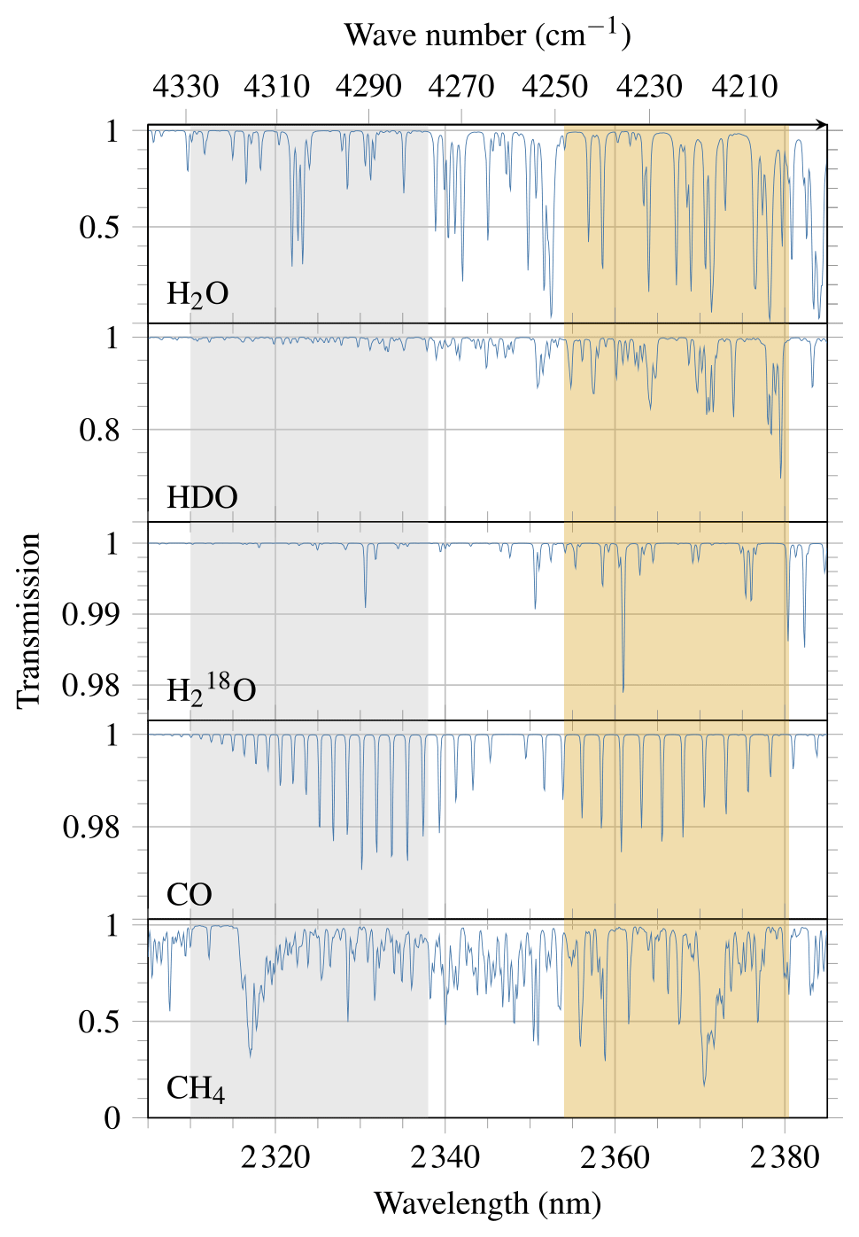
Figure 1Simulation of atmospheric transmission in the spectral range of TROPOMI's SWIR channel for the absorbers taken into account by the retrieval algorithm. The grey shading marks the spectral window used for the determination of effective cloud parameters, the yellow shading the spectral window for the retrieval of the trace gases.
A priori surface albedos are taken from a 1-year average over the year 2018 of the non-scattering product on an equal-area grid with 5760×2880 bins (corresponding to a resolution of 0.125∘ at the Equator). Values over oceans and lakes (where the non-scattering retrieval does not yield data) are set to 0 as water is very dark in the short-wave infrared. Figure 2 shows a map of this prior. To reduce interferences with cloud parameters and to stabilise the inversion, the surface albedo is slightly regularised to the prior. Regularisation in the context of ill-posed problems is discussed in detail by Borsdorff et al. (2014).
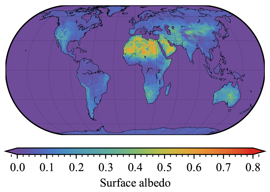
Figure 2Average surface albedo from the non-scattering retrieval (Schneider et al., 2020a) of the year 2018, which is used as a priori surface albedo for the scattering retrieval. Values over oceans and lakes (where the non-scattering retrieval does not yield data) are set to 0.
The results are filtered for convergence and with a quality filter based on fit quality in terms of the number of iterations and χ2 as a measure for the residual. Moreover, scenes with high solar zenith angles (SZAs) larger than 70∘ are filtered out since they are prone to errors. These errors are on the one hand due to multi-scattering and diffraction effects not covered well by the two-stream forward model and on the other hand due to typically low radiances resulting in low signal-to-noise ratios. From the remaining data, scenes are classified as clear sky, cloudy with low clouds, or other (e.g. high clouds) based on retrieved effective cloud parameters as specified in Table 1. Only scenes of the first two categories (i.e. clear sky or low clouds) are considered in this study and recommended to be taken into account by the user. If averaging kernels are taken into account, e.g. when assimilating the data, all scenes can be used, although shielding by high clouds may result in quite low information content. Clear-sky scenes are additionally filtered for surface albedo because low surface albedos usually involve low signal-to-noise ratios. Such a surface albedo filter is not applied to cloudy scenes because clouds usually have high reflectivity, which allows the retrieval algorithm to work over very low surface albedos with high signal-to-noise ratios.
Table 1Quality filters and selection criteria for clear-sky and cloudy-sky conditions.
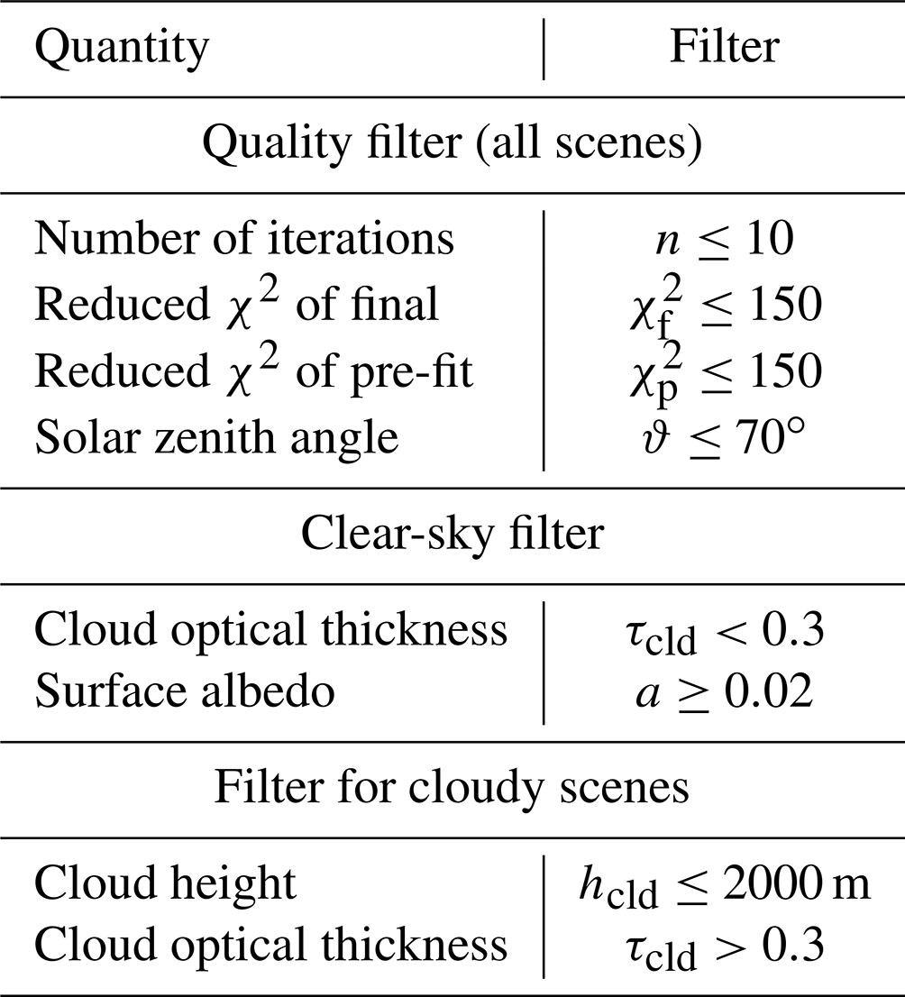
Figure 3 depicts a typical spectral fit. The root mean square (RMS) of the residual is somewhat higher than the nominal radiance precision; however, the latter only includes statistical noise in the detector signal but not errors due to correction (e.g. offset, dark current, memory, stray light) and conversion steps in the processor. This also leads to high χ2 values, particularly for bright scenes, e.g. over the Sahara region.
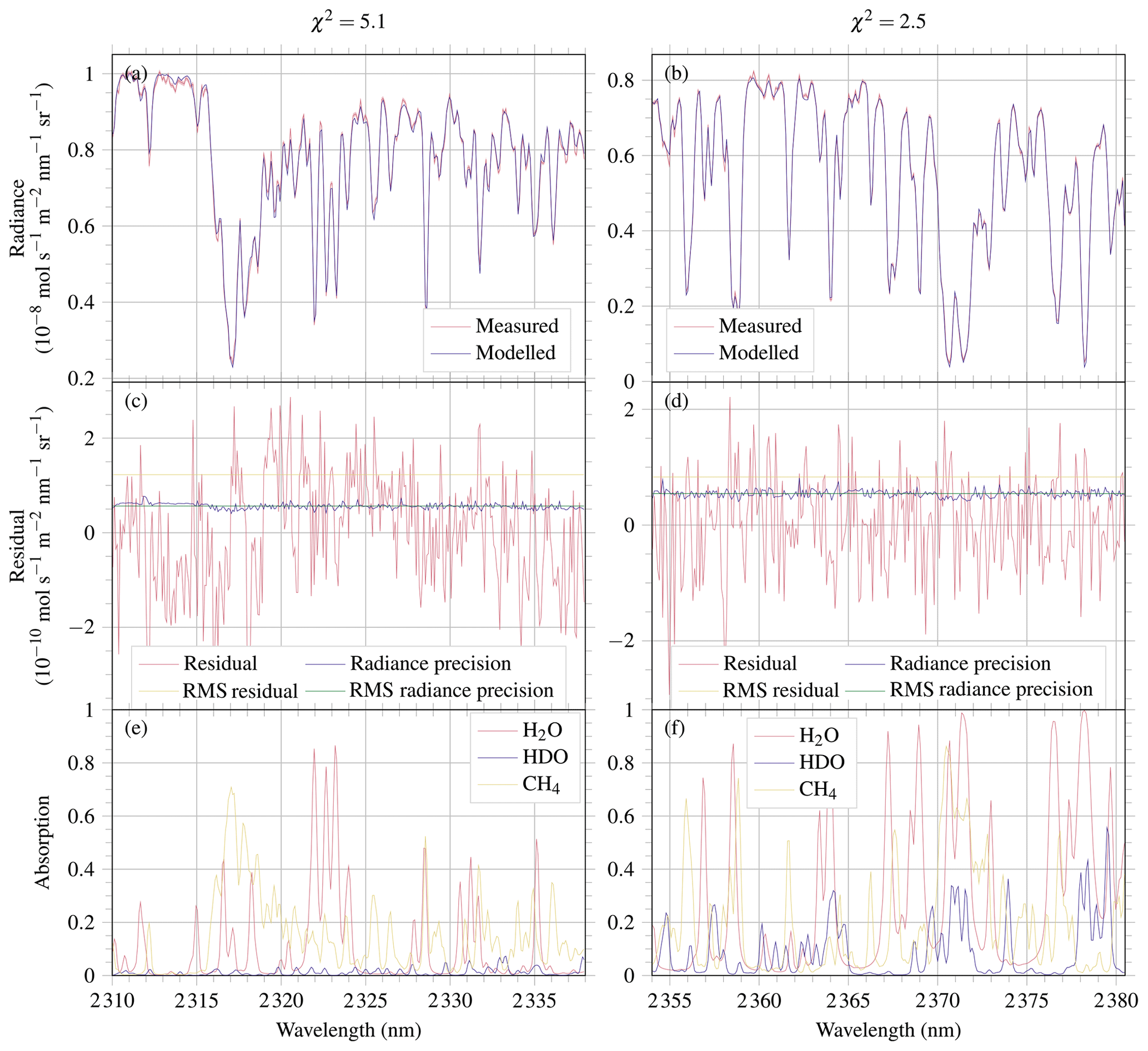
Figure 3Observed TROPOMI radiance (red) and spectral fit (blue) in (a) the pre-fit window and (b) the final window for ground pixel 511 754 in orbit 4924 located near Karlsruhe (7.8∘ E, 49.2∘ N) on 25 September 2018. Corresponding residuals (defined as measured minus modelled radiances, in red) and its root mean square (RMS, in yellow), precision of the radiance (in blue) and its RMS (in green) in (c) the pre-fit window and (d) the final window. Simulated absorption by H2O (red), HDO (blue) and CH4 (yellow) in (e) the pre-fit window and (f) the final window.
Retrievals over optically thick clouds are insensitive to the partial column below the cloud. The algorithm estimates the missing information from the prior, however, that can deviate from the truth. This requires a thorough data interpretation using the column averaging kernel, which indicates the vertical retrieval sensitivity. It can be used e.g. to assimilate the data with models to help with the interpretation when sensitivity is low.
3.1 Ground-based measurements by TCCON and co-location criteria
To validate the new satellite dataset, ground-based FTIR observations by the Total Carbon Column Observing Network (TCCON; Wunch et al., 2011), version GGG2014, are used. The TCCON HDO data are bias-corrected by dividing the HDO columns by a correction factor of 1.0778 as derived by Schneider et al. (2020a). This factor accounts for a missing aircraft correction factor of TCCON HDO. The aircraft correction factor corrects systematic biases due to uncertainties in the spectroscopy which tend to be highly reproducible (Wunch et al., 2015). It is usually obtained from a comparison to airborne reference measurements at TCCON sites, but such measurements are lacking for HDO. Thus, Schneider et al. (2020a) determined an effective factor by fitting TCCON a posteriori δD to MUSICA-NDACC δD because MUSICA-NDACC δD is validated with aircraft measurements.
Table 2 lists the stations that are used for the validation.
Strong et al. (2019)Notholt et al. (2019b)Kivi et al. (2014)Wunch et al. (2018)Deutscher et al. (2019)Notholt et al. (2019a)Hase et al. (2015)Té et al. (2014)Warneke et al. (2019)Sussmann and Rettinger (2018a)Sussmann and Rettinger (2018b)Wennberg et al. (2017)Morino et al. (2018c)Wennberg et al. (2016b)Morino et al. (2018a)Iraci et al. (2016)Wennberg et al. (2016a)Wennberg et al. (2015)Kawakami et al. (2014)Blumenstock et al. (2017)Morino et al. (2018b)Griffith et al. (2014)Sherlock et al. (2014)Pollard et al. (2019)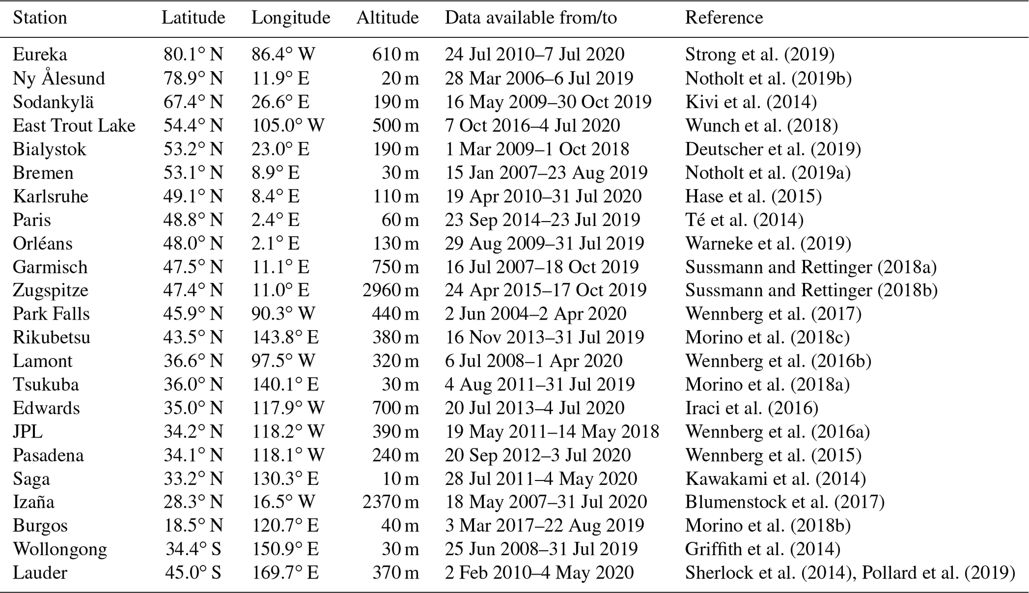
An FTIR instrument has sensitivity in its viewing direction (i.e. in the direction of the Sun). If the Sun is low in the sky (i.e. for high solar zenith angles), this translates into an azimuthal dependency of sensitivity, while there is no azimuthal dependency if the Sun is in the zenith. To take this into account, the spatial co-location considers satellite overpasses in a cone in the FTIR viewing direction with an opening angle α and a radius rα depending on solar zenith angle ϑ. Varying the opening angle linearly with SZA from at to 360∘ at and requiring an equal co-location area in all cases gives
Figure 4 illustrates this condition, which selects ground pixels depending on the directional sensitivity of the FTIR while keeping the co-location area constant. Here, is selected and r0 is computed from the radius at a solar zenith angle of 90∘, , with km. With these selections, the limit of gives the co-location criteria used for the validation of the non-scattering retrieval by Schneider et al. (2020a).
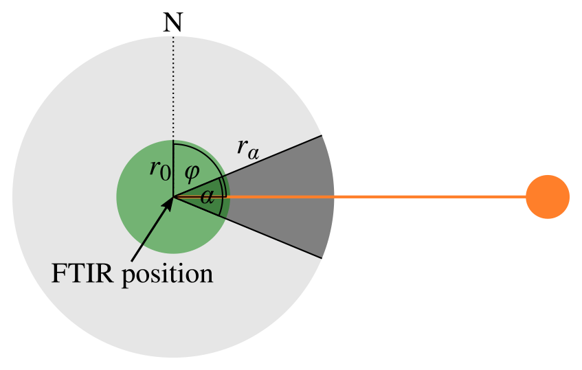
Figure 4Illustration of the spatial co-location condition. The co-location area consists of a cone in the FTIR viewing direction (i.e. solar azimuth angle φ) with opening angle α and radius rα depending on solar zenith angle ϑ (dark grey). The limit of is a full circle (green). The area remains constant (dark grey and green).
Additionally, the time between satellite and ground measurements has to be less than 2 h to minimise representation errors due to the diurnal cycle. Since the FTIR has to directly see the Sun (possibly through gaps in the clouds) to take measurements, co-located cloudy satellite observations require a change in the cloud cover within the co-location radius or the co-location time.
At low-altitude stations, i.e. stations below 1000 m above mean sea level (a.m.s.l.), only TROPOMI ground pixels with an altitude difference to the station height of less than 500 m are used. If the altitude difference between station and satellite ground pixel is too large, both observe too different partial columns, which leads to errors. That is the case for high-altitude stations that are typically located on mountains so that most co-located ground pixels have significantly lower surface height. Therefore, such stations are treated separately in Sect. 4.3.
The effects by different a priori profiles used by FTIR and satellite retrievals are accounted for with the column averaging kernel. Following Borsdorff et al. (2014), the adjustment of column ci retrieved using a priori profile xai to a priori profile xaj is performed with the column averaging kernel Ai of retrieval i by
where 1 is a vector with ones in all places. In the present case, i denotes TROPOMI and j denotes TCCON. TCCON a priori profiles are linearly interpolated from TCCON levels to SICOR layer centres, and the top layer is extended to 0 Pa to match the layering of the forward model. This correction is performed for all comparisons to TCCON data except for high-altitude stations.
3.2 Ground-based measurements by MUSICA-NDACC
The project MUlti-platform remote Sensing of Isotopologues for investigating the Cycle of Atmospheric water (MUSICA; Schneider et al., 2016; Barthlott et al., 2017) also provides a ground-based water vapour isotopologue data product, which uses spectra measured within the Network for the Detection of Atmospheric Composition Change (NDACC; De Mazière et al., 2018). Two different products exist, firstly the direct retrieval output, called the type-1 product, and secondly an a posteriori processed output that reports the optimal estimation of (H2O, δD) pairs, called the type-2 product. Here, the type-2 product is used because it is recommended for isotopologue analyses (Barthlott et al., 2017). Recent MUSICA-NDACC data are currently only available for three stations (Karlsruhe, Kiruna and Izaña), which compromise globally valid validation studies.
Seven stations are in both networks, TCCON and NDACC. In these cases, the TCCON and NDACC measurements are performed with the same instrument but in a different spectral range at different times. As shown e.g. by Schneider et al. (2020a), the retrievals from the two networks do not agree.
Based on the fact that MUSICA δD is calibrated by aircraft measurements near Izaña but that TCCON HDO is not verified, Schneider et al. (2020a) derived a correction of TCCON HDO by matching TCCON a posteriori δD to MUSICA-NDACC δD. Nevertheless, H2O columns also differ between TCCON and MUSICA-NDACC. Since TCCON H2O is better validated and thus assumed to be correct, this discrepancy is solved by a correction of MUSICA-NDACC derived in the following. Figure 5a shows correlations of TCCON and MUSICA-NDACC H2O columns at Wollongong, Australia. The difference is well described by a simple scaling of the column. The result of such a fit for all stations in both networks (as listed in Table 3) is presented in Fig. 5c. The correction factors do not vary considerably between stations. To harmonise both datasets, MUSICA H2O and HDO columns are thus corrected by division by the mean correction factor 1.1527 (red line in Fig. 5c). This adjusts the MUSICA H2O columns while leaving MUSICA δD unchanged. This correction is applied to all MUSICA-NDACC stations, i.e. also those not in TCCON.
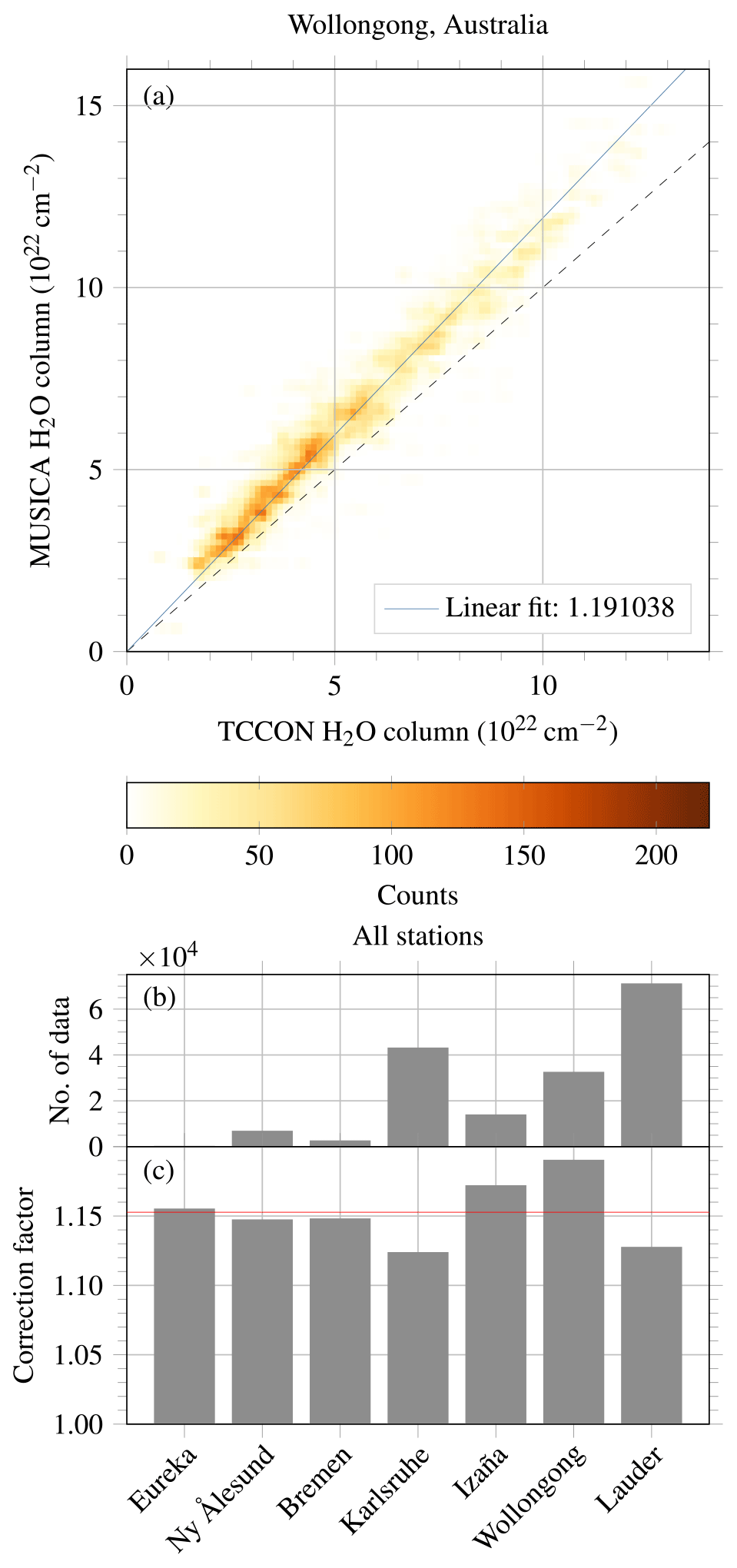
Figure 5(a) Two-dimensional histogram of correlations of co-located TCCON and MUSICA-NDACC H2O columns at Wollongong (colour-coded) and the result of a fit of a linear correction (blue line). The one-to-one line is shown dashed. (b) Number of co-located observations for all individual stations in both networks. (c) Correction factors to correct MUSICA-NDACC H2O columns to TCCON. The average 1.1527 is marked by a red line.
Filling the null space of TROPOMI measurements with MUSICA-NDACC a priori profiles with averaging kernels creates large scatter and deviations from the reference. MUSICA a priori profiles do not depend on time and are much less realistic than TCCON or TROPOMI a priori profiles. This can lead to deviations. Thus, averaging kernels are not applied for the validation with MUSICA-NDACC data.
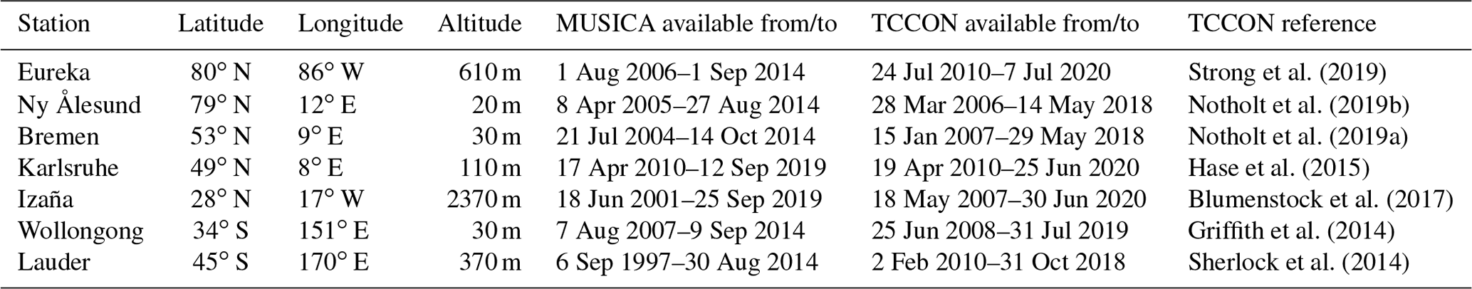
Strong et al. (2019)Notholt et al. (2019b)Notholt et al. (2019a)Hase et al. (2015)Blumenstock et al. (2017)Griffith et al. (2014)Sherlock et al. (2014)Table 3List of ground stations used for the derivation of the FTIR correction.
3.3 Aircraft measurements
During the NASA ObseRvations of Aerosols above CLouds and their intEractionS (ORACLES) field mission in the south-eastern Atlantic Ocean region (Redemann et al., 2021), measurements of H2O mixing ratio and δD were taken onboard the NASA P-3B Orion aircraft with the Water Isotope System for Precipitation and Entrainment Research (WISPER) instrument (Henze et al., 2021). This instrument employs in situ gas-phase cavity ring-down water vapour isotopic analysers (Picarro model L2120-fi) coupled to inlets that enable paired measurements of cloud water, total water amounts and isotope ratios.
The validation uses profile measurement data from the 2018 field mission. Only profiles reaching at least 5000 m are taken into account. For ascent profiles, descending sections are filtered out by discarding sections with higher pressure than a previous data point; similarly, ascending sections are removed from descent profiles. If more than 30 % of the data are discarded in this step, the whole profile is dropped. This eliminates flight sections with a “saw-tooth” pattern designed for sampling in cloudy regions. Altogether, 17 profiles pass the filter, spanning the time range from 27 September 2018 to 21 October 2018. The top altitude varies between 5130 and 7408 m with an average of 6195 m. The vertical resolution is typically 30 m due to sampling at 1 Hz and typical aircraft descent rates. HDO mixing ratios are computed from H2O mixing ratios and δD. In order to derive total columns, the aircraft profiles are extended to the ground by assuming a constant mixing ratio equal to the lowest observed value and extended to the top with the scaled prior profile. These extended profiles are then vertically integrated to obtain total columns.
The co-location is performed with the full 360∘ viewing angle (as the in situ instrument does not have a directional sensitivity like the FTIR) and a radius of 10.6066 km (corresponding to the radius for the full circle r0 in Sect. 3.1). For each co-located measurement, the satellite a priori profile is scaled such that the partial column below the ceiling of the aircraft profile coincides with that of the aircraft measurement. The aircraft profile is interpolated to the grid of the a priori profile, and the part above the ceiling is complemented by the upper part of the scaled a priori profile. Finally, the averaging kernel Ai of the satellite measurement is applied to compute the smoothed reference column by
which is then used for the validation.
In the following subsections, the scattering retrieval is validated for clear-sky and cloudy scenes according to retrieved effective cloud parameters as described in Sect. 2. As a reference, the plots additionally show the non-scattering retrieval filtered as reported by Schneider et al. (2020a), i.e. with the cloud fraction from the Visible Infrared Imaging Radiometer Suite (VIIRS) co-located to the TROPOMI field of view, a two-band filter as described in Schneider et al. (2020a), and the solar zenith angle.
4.1 Low-altitude stations
Figure 6 depicts an exemplary time series of daily medians of co-located measurements at the TCCON station Karlsruhe. The TROPOMI observations follow the reference well, although some deviations are present, especially for cloudy scenes.

Figure 6Time series of (a) individual observations per day, (b) daily medians of H2O columns, (c) HDO columns and (d) a posteriori δD of TCCON (grey), TROPOMI clear-sky scenes (blue), TROPOMI cloudy scenes (yellow) and the former TROPOMI non-scattering retrieval (red) at Karlsruhe, Germany (49.1∘ N, 8.4∘ E, 110 m a.m.s.l.).
Figure 7 presents corresponding correlations. Retrieved columns correlate excellently with the reference, with Pearson correlation coefficients of 0.98 in H2O and 0.99 in HDO for clear-sky scenes and 0.95 in H2O and 0.96 in HDO for cloudy scenes. A posteriori δD has more scatter, with correlation coefficients of 0.86 and 0.83 for clear-sky and cloudy scenes, respectively. The bias, which is defined as the mean difference between TROPOMI and TCCON, is for clear-sky scenes molec cm−2 (−0.4 %) in H2O and molec cm−2 (−1.0 %) in HDO, which corresponds to a bias in a posteriori δD of −3 ‰ (1.1 %). For cloudy scenes, it is 4.9×10²¹ molec cm−2 (8.3 %) in H2O, 1.1×10¹⁸ molec cm−2 (6.5 %) in HDO and −12 ‰ (7.3 %) in a posteriori δD. The retrieval performance for cloudy scenes is good: correlations are similar to clear-sky scenes or the non-scattering retrieval, although the bias is larger. This can be explained by the small sensitivity of the retrieval below optically thick clouds.
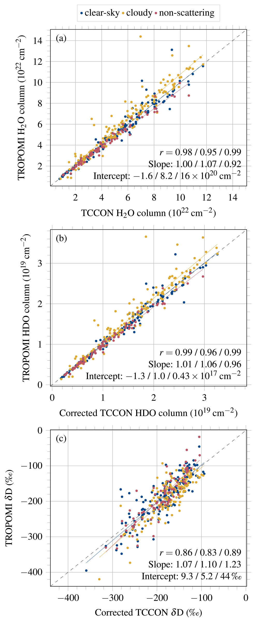
Figure 7Correlations of TROPOMI observations against corrected TCCON measurements of (a) H2O columns, (b) HDO columns and (c) a posteriori δD for clear-sky scenes (blue), cloudy scenes (yellow) and the non-scattering retrieval (red) at Karlsruhe. The coloured lines represent linear fits and the dashed line denotes the one-to-one line.
Figure 8 presents statistics and correlation coefficients of daily medians at all low-altitude stations. The amount of data for clear-sky scenes of the new scattering retrieval is much larger than for the old non-scattering retrieval, on average a factor of 8 more. This is explained by different filtering: while the non-scattering product is strictly filtered with the S5P-VIIRS product and an additional two-band filter (Schneider et al., 2020a), the scattering product is filtered with effective cloud parameters retrieved in the pre-fit (see Table 1). The number of observations (ground pixels) per day (Fig. 8b) is usually around four but is significantly higher at high latitudes due to multiple overpasses per day. Cloudy scenes encounter typically fewer observations per day compared to clear-sky scenes, with a median of 3.4 vs. 4.1. The non-scattering retrieval has a significantly lower data yield, with a median of 2.7 co-located ground pixels per day. The distributions visualised by the violin plots show that there is quite some spread, with some days with a high number of observations.
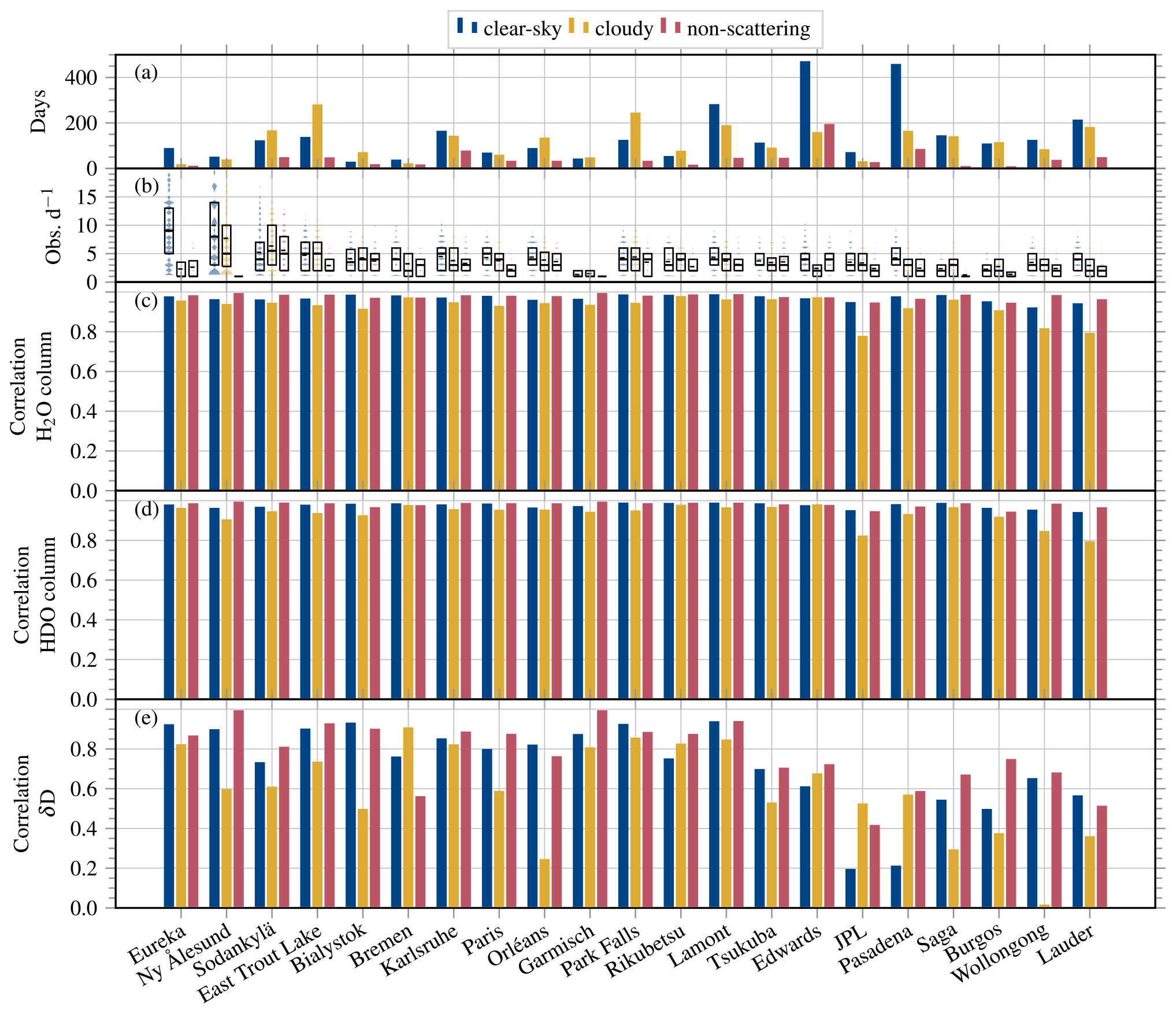
Figure 8(a) Number of days with observations, (b) observations per day, (c) correlation coefficients of H2O columns, (d) correlation coefficients of HDO columns and (e) correlation coefficients of a posteriori δD at all TCCON stations.
Correlations of daily medians of H2O and HDO columns are excellent at all stations (Fig. 8c, d). In a posteriori δD, correlations are lower at some stations, typically ones with low seasonal variation (Fig. 8e). For clear-sky scenes, correlation coefficients are similar to those of the non-scattering product, except for δD at some stations like the Jet Propulsion Laboratory (JPL) and Pasadena. For cloudy scenes, the correlations are mostly slightly lower than for clear-sky scenes.
Biases are depicted in Fig. 9. At low and middle latitudes the bias is generally small: at these stations, the median for clear-sky scenes is 1.3×10²¹ molec cm−2 (1.8 %) in H2O columns, 2.0×10¹⁶ molec cm−2 (−0.3 %) in HDO columns and −8 ‰ (4.6 %) in δD, and the one for cloudy scenes is 4.7×10²¹ molec cm−2 (8.8 %) in H2O columns, 1.1×10¹⁸ molec cm−2 (6.5 %) in HDO columns and −20 ‰ (12 %) in δD. High-latitude stations mostly have larger biases that can be as high as 20 % in the columns and 40 ‰ in a posteriori δD. The median bias at high-latitude stations (Eureka, Ny Ålesund, Sodankylä, and East Trout Lake) in H2O, HDO and δD is for clear-sky scenes 2.3×10²¹ molec cm−2 (9.5 %), 4.0×10¹⁷ molec cm−2 (0.4 %) and −37 ‰ (13 %) and for cloudy scenes 5.1×10²¹ molec cm−2 (12 %), 1.0×10¹⁸ molec cm−2 (9.1 %) and −24 ‰ (8.4 %), respectively. These high biases are similar but partly more pronounced than for the non-scattering retrieval. High-latitude locations employ difficult measurement geometries with typically high solar zenith angles and low surface albedos, in which the additional estimation of cloud parameters seems to be even more challenging. In summer, these biases are typically lower than in darker seasons with higher solar zenith angles. The bias is also high at Garmisch, which lies in a mountainous region, meaning a complex topography with typically large variation in surface altitude and albedo within a ground pixel. The median bias of all stations is for clear-sky scenes 1.4×10²¹ molec cm−2 (2.9 %) in H2O columns, 1.1×10¹⁷ molec cm−2 (−0.3 %) in HDO columns and −17 ‰ (9.9 %) in a posteriori δD. For cloudy scenes, it is 4.9×10²¹ molec cm−2 (11 %) in H2O, 1.1×10¹⁸ molec cm−2 (7.9 %) in HDO and −20 ‰ (9.7 %) in a posteriori δD. Although the absolute bias in δD is higher for cloudy scenes than for clear-sky scenes, the relative bias is not. This is connected to different conditions in cloudy and clear-sky weather. The distributions of the differences (TROPOMI − TCCON, visualised by the violin plots in Fig. 9) vary considerably between stations. Outliers are present, which shows that statistics over an adequate amount of data are needed for interpretation. Altogether, the performance of the new scattering retrieval for clear-sky scenes is similar to the one of the non-scattering retrieval, even though the scattering retrieval yields much more data. Biases are slightly smaller in HDO but slightly larger in a posteriori δD.
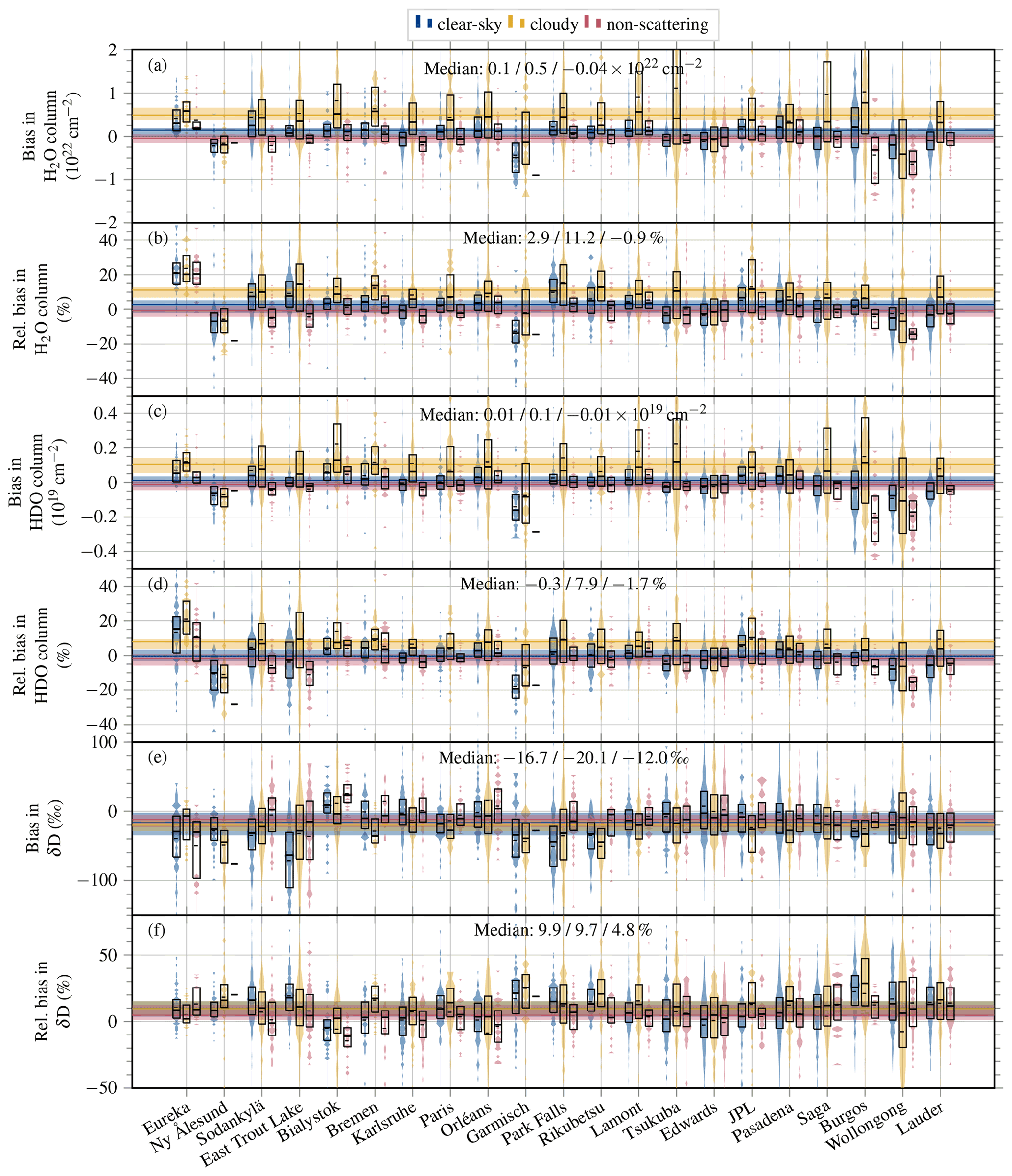
Figure 9(a) Bias in H2O columns, (b) relative bias in H2O columns, (c) bias in HDO columns, (d) relative bias in HDO columns, (e) bias in δD, and (f) relative bias in δD for clear-sky scenes (blue), cloudy scenes (yellow) and the non-scattering retrieval (red). The violin plots visualise the distributions of differences between TROPOMI and TCCON, the boxplots mark quartiles and the dashed lines inside the boxes mark the mean. Coloured horizontal lines denote station-to-station medians and the shading around them the station-to-station quartiles.
4.2 Comparison to the former non-scattering dataset
For a direct comparison of the new scattering retrieval to the former non-scattering retrieval by Schneider et al. (2020a), only ground pixels for which both retrievals yield valid data are considered. Figure 10 shows distributions of the differences to the reference (TROPOMI − TCCON) for the same ground pixels. It demonstrates that both retrievals perform similarly at most low-altitude TCCON stations at middle and low latitudes. Significant differences are only present at the coastal stations Burgos and Wollongong and at Park Falls. The station-to-station median bias for this scene selection at low- and mid-latitude stations is in H2O 4.4×10²⁰ molec cm−2 or 0.3 % for the scattering retrieval vs. molec cm−2 or 0.4 % for the non-scattering retrieval and in HDO molec cm−2 or −1.1 % vs. molec cm−2 or −1.3 %. In a posteriori δD it is −14 ‰ (7.5 %) for the scattering retrieval vs. −11 ‰ (5.4 %) for the non-scattering retrieval. This demonstrates that the performance of both retrievals is comparable under clear-sky conditions.
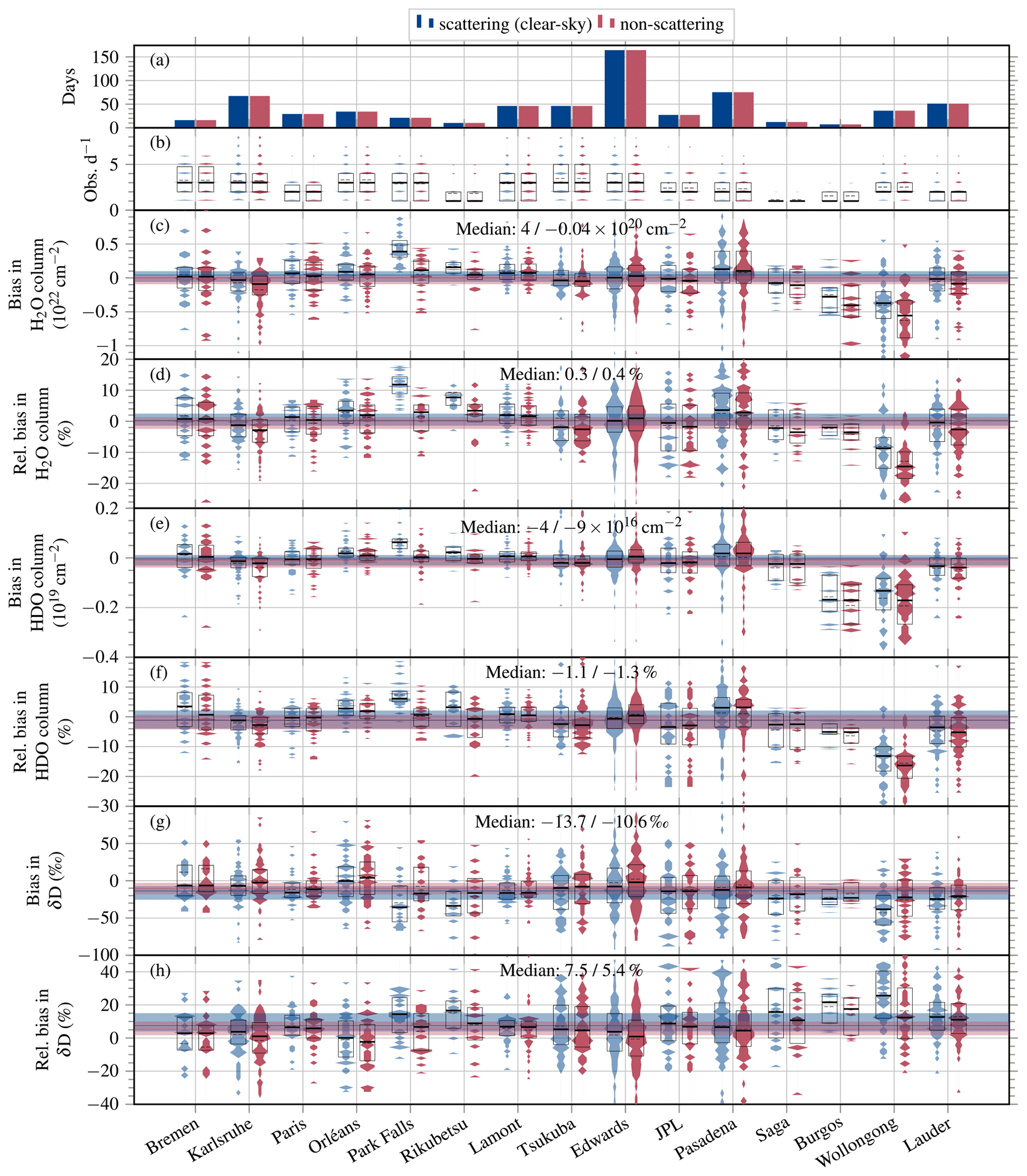
Figure 10(a) Number of days with observations, (b) observations per day, (c) bias in H2O columns, (d) relative bias in H2O columns, (e) bias in HDO columns, (f) relative bias in HDO columns, (g) bias in δD, and (h) relative bias in δD for the scattering retrieval (blue) and the non-scattering retrieval (red). The violin plots visualise the distribution of differences between TROPOMI and TCCON, the boxplots mark quartiles and the dashed lines inside the boxes show the mean. Coloured horizontal lines denote station-to-station medians and the shading around them the station-to-station quartiles.
4.3 High-altitude stations
Ground stations on high mountains are special because the station height and the mean surface altitude of co-located satellite ground pixels typically differ considerably, which means that different air columns are observed by both. This leads to high biases if not accounted for. Therefore, the chosen prior plays an important role in this situation. To demonstrate the role of the prior in potential corrections, an additional run with HDO a priori profiles obtained by an assumed more realistic δD profile as described in Sect. 2 has been performed. This prior is referred to as a “depleted” prior because a depletion in HDO is assumed to compute it from the humidity profile. The standard prior is also referred to as a “scaled” prior because it consists of a scaled humidity profile (i.e. corresponding to 0 ‰ δD). During the co-location, the same ground pixels are considered for both runs. Moreover, averaging kernels are not applied for this analysis because the a priori profiles of the retrieval are used for the altitude correction.
The left column of Fig. 11 demonstrates the high biases of uncorrected clear-sky observations near Zugspitze (2964 m a.m.s.l.), which for the standard prior amount to 185 % in H2O, 232 % in HDO and 75 ‰ in δD. Nevertheless, the time series does follow the relative variability of the reference.
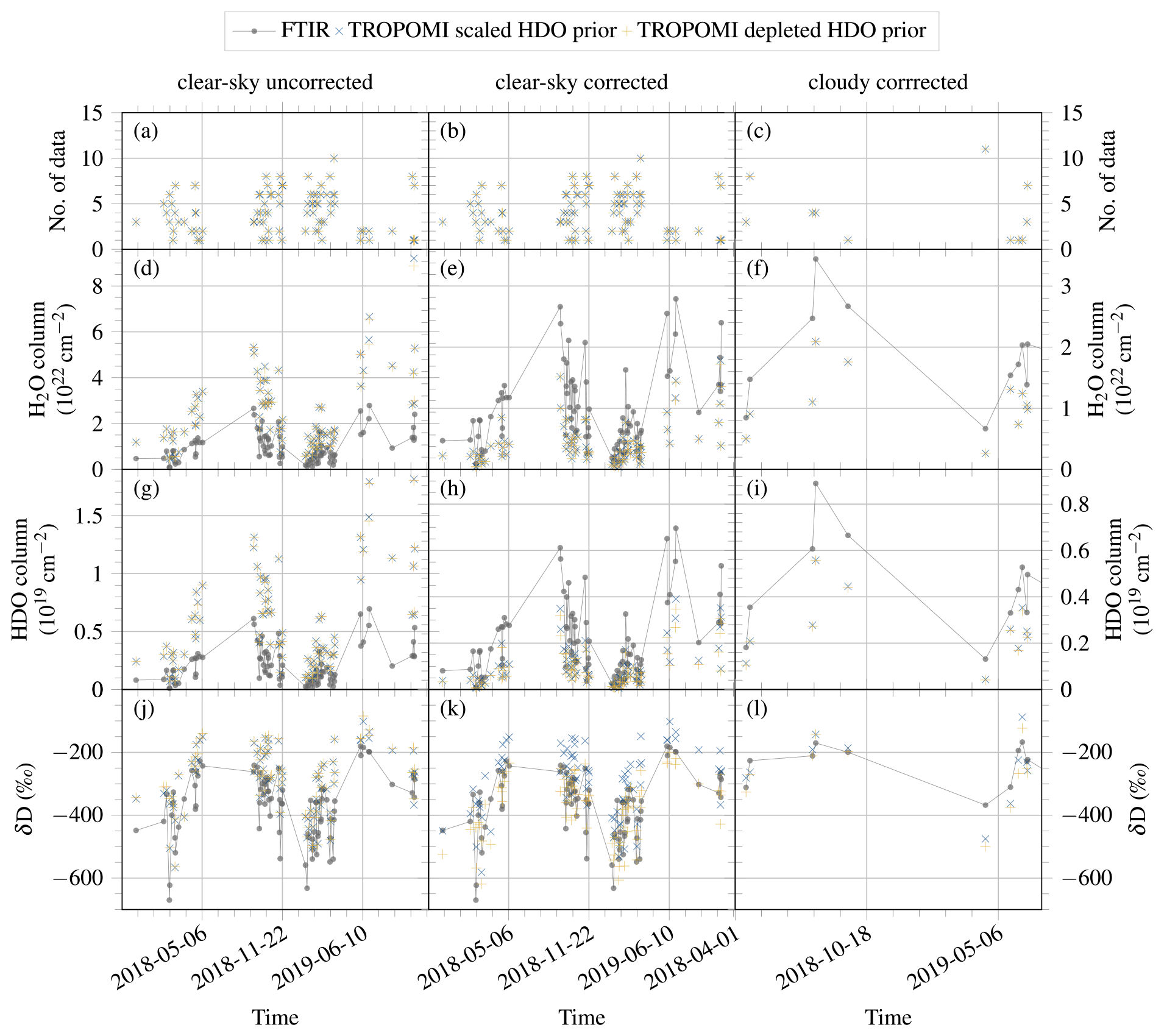
Figure 11Time series of (a–c) the number of individual measurements per day, (d–f) bias in the H2O column, (g–i) bias in the HDO column, and (j–l) bias in δD at the high-altitude station Zugspitze (2964 m a.m.s.l.). The left panels (a), (d), (g) and (j) show clear-sky measurements without altitude correction, the centre panels (b), (e), (h) and (k) show the same measurements with altitude correction, and the right panels (c), (f), (i) and (l) show observations over optically thick clouds within an altitude range 1000 m above and 500 m below the station height. Please note that in the left panels the H2O and HDO axes are different than in the centre and right panels, as indicated by the axis ticks. The blue points correspond to the standard prior which is scaled from the humidity profile, while the yellow points correspond to the prior computed assuming a more realistic δD profile.
The ground station on top of the mountain is always higher than the (mean) ground pixel altitude. To correct for the altitude differences, the partial columns of the TROPOMI observations above the station height are considered by truncating the scaled profile of the retrieval at the altitude of the station. This is the same procedure as applied by Schneider et al. (2018, Sect. 4). The second column of Fig. 11 depicts the resulting time series. The bias in both H2O and HDO is greatly reduced to −54 % and −48 % for the standard prior and −55 % and −54 % for the depleted prior. In a posteriori δD a large difference between both priors is visible: while the bias for the scaled prior is practically the same as for the uncorrected case, 73 ‰, it is largely reduced to 4 ‰ for the depleted prior. The first is due to the fact that the altitude correction in H2O and HDO cancels out when dividing HDO by H2O if the same profile shapes are used. On the other hand, the small bias in δD in the second case shows that the assumed depleted HDO profile shape is indeed a good estimate for this case.
Table 4Filter criteria for cloudy-sky scenes at high-altitude stations. Here hs denotes the height of the ground site.
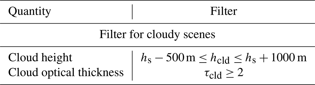
Another possibility is to utilise the shielding of clouds. To this end, scenes with optically thick clouds at an altitude similar to the station height as specified in Table 4 are selected. In these cases, the satellite measurement is sensitive above the cloud but insensitive below the cloud. Figure 12 illustrates the corresponding averaging kernels for a clear-sky scene and a cloudy scene.
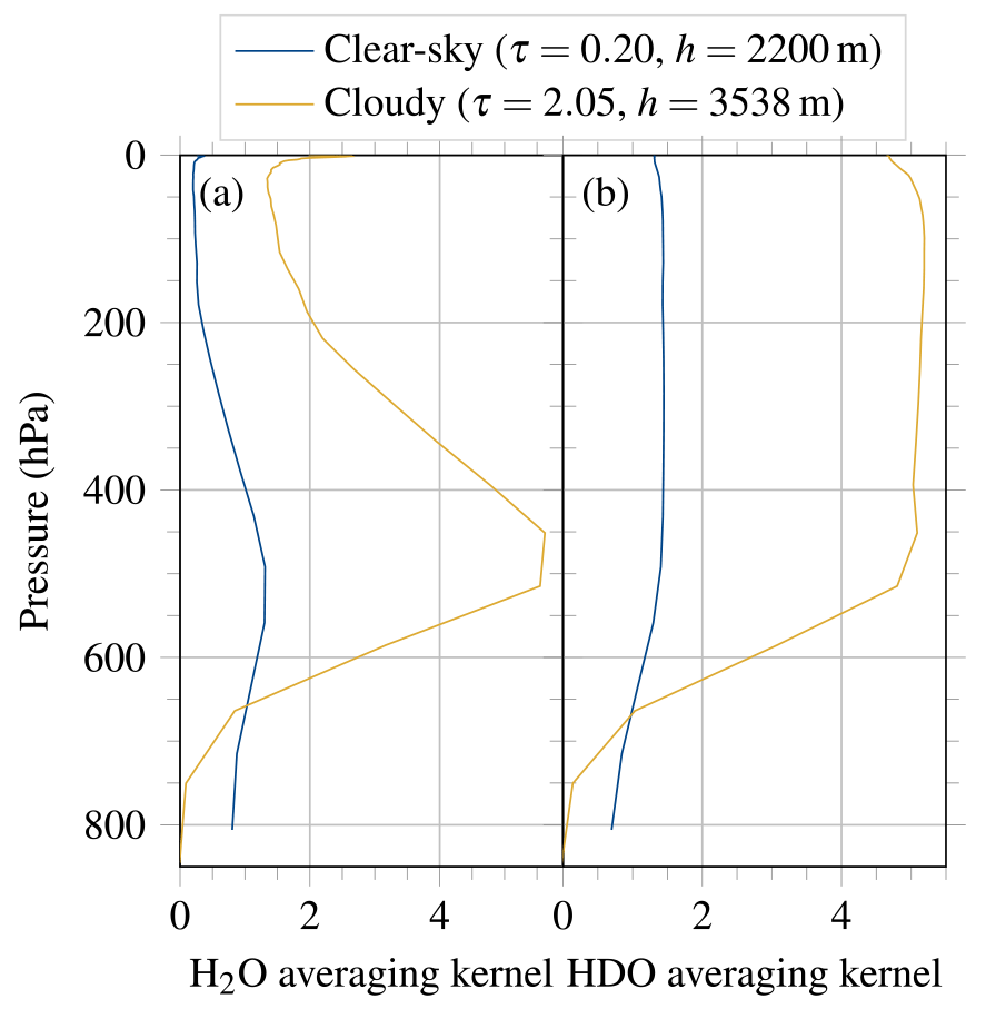
Figure 12Averaging kernels of (a) H2O and (b) HDO for a clear-sky scene (orbit 4725 on 11 September 2018, blue) and a cloudy scene (orbit 4839 on 19 September 2018, yellow) near Zugspitze.
Since the FTIR has to see the Sun and thus can measure only through gaps in the clouds or when the cloud cover changes within the co-location time, the amount of data for cloudy scenes is very small. Thus, the co-location radius is extended to km in this case. The inferred columns are corrected for the altitude difference between ground pixel and station height as described above. The right panel of Fig. 11 depicts the resulting time series. The biases in the columns and in a posteriori δD are acceptable for both priors. They amount to 4 ‰ for the scaled prior and −24 ‰ for the depleted prior. That the shielding yields good agreement with the scaled prior shows that the data provide information about the vertical distribution.
Figure 13 depicts biases for both high-altitude stations Zugspitze and Izaña. It confirms the behaviour seen in the time series at Zugspitze for both stations. Uncorrected clear-sky observations yield a large bias in all quantities. The altitude correction greatly reduces the bias in the H2O and HDO columns. In δD, the correction cancels out when assuming the same vertical distributions of H2O and HDO, so that the bias remains. However, the altitude correction with a more realistic prior yields a substantial reduction of the bias in δD. For cloudy scenes with optically thick clouds at similar altitudes to the station height, the biases are also relatively small, although the validation is hampered by a small amount of data.
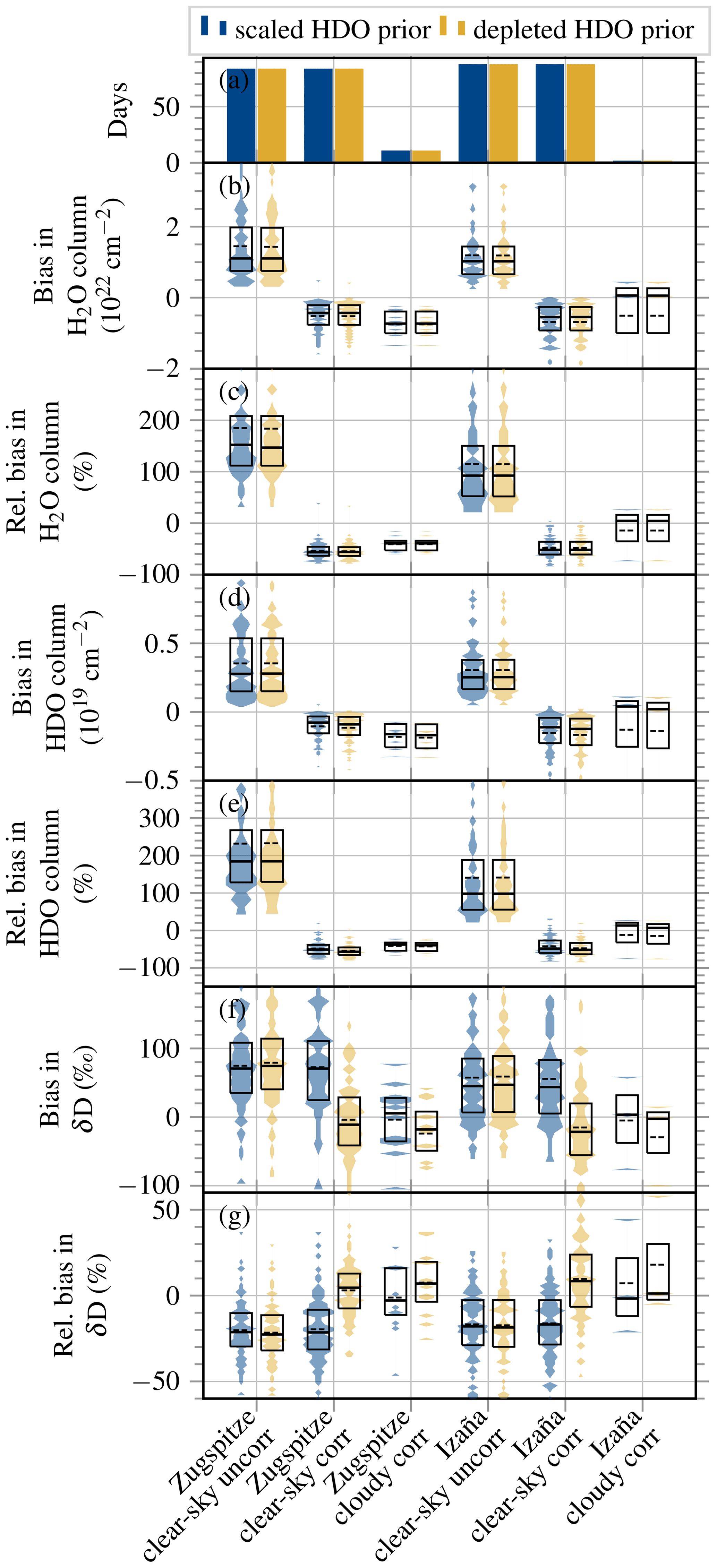
Figure 13Biases for high-altitude TCCON stations plotted similarly to Fig. 9 but for retrievals with the standard scaled HDO a priori profile (blue) and an HDO a priori profile obtained by assuming a more realistic δD profile described in Sect. 2 (yellow). Shown are (a) the number of days with observations, (b) the bias in H2O columns, (c) the relative bias in H2O columns, (d) the bias in HDO columns, (e) the relative bias in HDO columns, (f) the bias in δD, and (g) the relative bias in δD. For each station, three entries are shown which correspond to uncorrected clear-sky observations, clear-sky observations corrected for the station altitude and altitude-corrected cloudy observations.
4.4 MUSICA-NDACC
Recent MUSICA-NDACC data are available for two low-altitude stations. Karlsruhe is also in TCCON, so that a comparison is possible. MUSICA-NDACC provides fewer measurements than TCCON (113 vs. 170 for clear-sky scenes and 83 vs. 148 for cloudy scenes). This is, among others, due to longer durations of individual FTIR measurements for NDACC compared to TCCON. Correlations, as shown in Fig. 14, are excellent in the retrieved columns. For clear-sky scenes, Pearson correlation coefficients are 0.98 in H2O and 0.99 in HDO, the same numbers as derived for TCCON (compare Fig. 7). For cloudy scenes, correlations with MUSICA-NDACC are at 0.98 in H2O and 0.99 in HDO even better than with TCCON, with however considerably fewer data points. A posteriori δD also has excellent correlation coefficients of 0.93 for clear-sky scenes and 0.91 for cloudy scenes, which is better than with TCCON. The bias for clear-sky scenes is 1.8×10²¹ molec cm−2 (2 %) in H2O, 2.5×10¹⁷ molec cm−2 (−0.1 %) in HDO and −16 ‰ (8.4 %) in δD. For cloudy scenes, the bias is 6.4×10²¹ molec cm−2 (9.9 %) in H2O, 9.3×10¹⁷ molec cm−2 (4.8 %) in HDO and −37 ‰ (21 %) in δD. This is significantly larger than for TCCON.
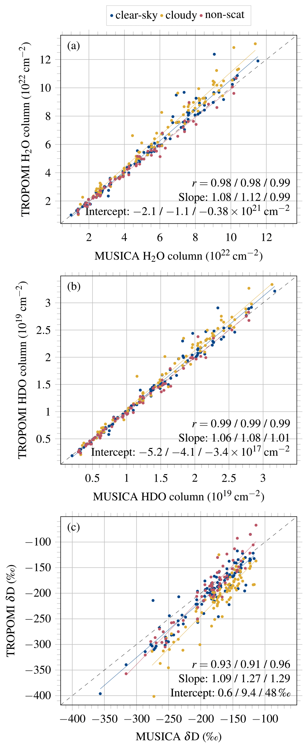
Figure 14Correlations of TROPOMI observations against corrected MUSICA-NDACC measurements of (a) H2O columns, (b) HDO columns and (c) a posteriori δD for clear-sky scenes (blue), cloudy scenes (yellow) and the non-scattering retrieval (red) at Karlsruhe. The coloured lines represent linear fits and the dashed line denotes the one-to-one line.
Only one other low-altitude station provides MUSICA-NDACC data with temporal overlap with the TROPOMI mission, namely Kiruna. This is a high-latitude station, so that high biases are expected due to difficult retrieval conditions with high solar zenith angles and low surface albedos (cf. Sect. 4.1). They amount to 2.6×10²¹ molec cm−2 (4.6 %) in H2O, 1.6×10¹⁷ molec cm−2 (−3.5 %) in HDO and −58 ‰ (24 %) in δD for clear-sky scenes and 5.0×10²¹ molec cm−2 (12 %) in H2O, 6.4×10¹⁷ molec cm−2 (5.1 %) in HDO and −51 ‰ (23 %) in δD for cloudy scenes. With only two stations, it is not meaningful to make statistical statements.
4.5 WISPER aircraft measurements over the ocean
In order to validate the retrievals over oceans, aircraft profiles from the ORACLES field campaign in 2018 are used as a reference. The co-location method is described in Sect. 3.3.
Figure 15 shows a time series of total columns computed from aircraft profiles and co-located TROPOMI retrievals over the North Atlantic Ocean. The bias is molec cm−2 or % in H2O and ‰ in δD. The validation over the ocean is hampered by very few data points. Nevertheless, the comparison to the available aircraft profiles shows a good performance of the retrieval over the ocean.
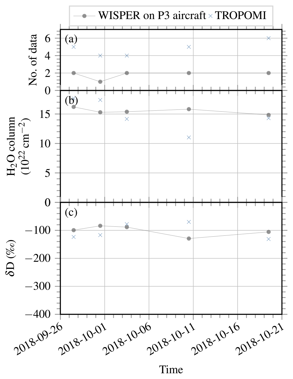
Figure 15Time series of (a) the number of measurements, (b) daily averaged total columns of H2O and (c) δD from aircraft profiles (grey) and co-located TROPOMI retrievals (blue).
5.1 Global picture
Figure 16 demonstrates a global picture of the new dataset with a monthly average for September 2018. The most prominent improvement compared to the same figure for the non-scattering product shown in Schneider et al. (2020a, Fig. 10) is a huge enhancement in data coverage, most prominently over the oceans and in regions at low latitudes with persistent clouds (e.g. over the Amazon, central Africa and Oceania), where the non-scattering retrieval yields no data. Near these regions and also over northern India, δD is lower than in the non-scattering (clear-sky-only) data product, which is attributed to different weather conditions on cloudy days compared to clear-sky days.
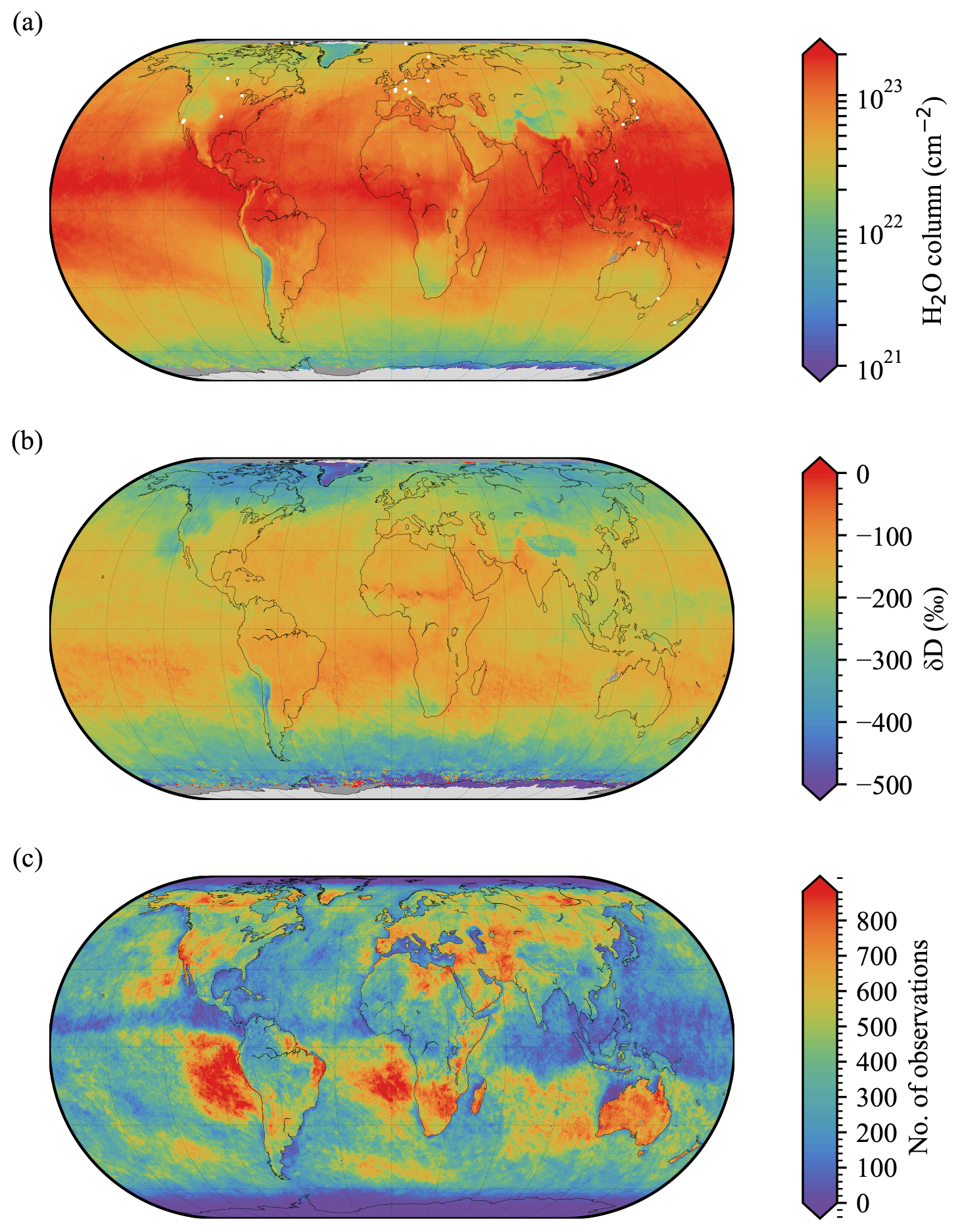
Figure 16Global plots of (a) average H2O, (b) average δD, and (c) number of observations for September 2018 on a grid. The average of δD is weighted with the H2O column. The white points in (a) show the locations of the TCCON stations used for validation in Sect. 4.1.
The data coverage, as can be seen in the example for the month of September 2018 in Fig. 16c, is highly variable in space. Particularly over tropical oceanic regions, the data are still very sparse due to shielding by high clouds. Over high-latitude land regions, the data are also still sparse due to high solar zenith angles and low surface albedos (recall the SZA filter and albedo filter; cf. Table 1). In contrast, particularly in regions of enhanced subsidence in the subtropics, a large number of observations are available.
The distribution of the (H2O, δD) pairs in the tropics is shown in Fig. 17 for September 2018 to give a first insight into the benefit from δD compared to only H2O total column information. A large variability is observed in total column δD at high humidity levels (−200 ‰ to −100 ‰), which may be controlled by the strength of convection and the level of convective aggregation in different regions (Fig. 17). Furthermore, the δD distributions show the highest occurrence frequencies at higher δD over land ( ‰) than ocean ( ‰), while H2O is higher over ocean (6000–8000 ppm) than land (2000–4000 ppm). This might reflect differences in properties of deep convective system organisation and/or the impact of continental cycling, which highlights the value of total column δD for process-based studies of the atmospheric water cycle in the tropics.
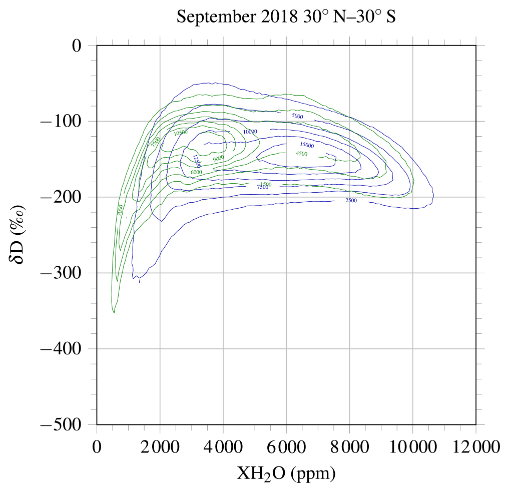
Figure 17(H2O, δD) phase space for all valid measurements in September 2018 in the latitude band 30∘ N–30∘ S. Green isolines correspond to data over land and blue isolines to data over oceans.
5.2 Single overpasses
Figure 18 demonstrates single-overpass results over the North Atlantic Ocean. On 17 January 2020 a cold air outbreak forms along the North American eastern coast behind a cold front associated with a North Atlantic cyclone. The cold front can be identified in Fig. 18a by the quasi-zonal cloudy band, marked by a strong gradient of low to high total column H2O between 15 and 25∘ N across the front. The cold air mass (see low values of potential temperature at 850 hPa behind the cold front in Fig. 18f) travels southward towards the tropics between 17 and 20 January 2020 (Figs. 18–20). The cold, subsiding air behind the cold front is very dry (Fig. 18a) and is associated with low total column δD values between −400 ‰ and −200 ‰ (Fig. 18b) which are characteristic of the cold sector of extratropical cyclones (Thurnherr et al., 2021). Marine cold air outbreak clouds are typically low-level clouds with a high cloud fraction (stratocumulus, cumulus, Fig. 18e) and moderate optical thickness (Fig. 18c, Fletcher et al., 2016). The very high δD values of ∼0 ‰ stretching in a bow from ∼20∘ N, 40∘ W westward are caused by low sensitivity at low altitudes due to cloud shielding. These sensitivity issues are reflected by very low values of the column averaging kernel (Fig. 18d). The magnitude of the null-space error is determined by the deviation of the shape of the a priori profile to the real profile. The prior depends on time and location, and thus the null-space error may be different in different regions. Nevertheless, these TROPOMI data still contain valuable information that can be interpreted in combination with measurements or model simulations providing vertical profiles of H2O and HDO that can be combined with the vertical sensitivity of the satellite retrievals.

Figure 18TROPOMI single-overpass results of (a) XH2O, (b) δD, (c) retrieved effective cloud optical thickness and (d) column averaging kernel at the surface over the North Atlantic on 19 January 2020; (e) ERA5 cloud fraction and (f) ERA5 potential temperatures at 850 hPa at 15:00 UTC. The grey contours in all panels show ERA5 mean sea-level pressure at 15:00 UTC with a contour line distance of 2 hPa. The black contours in (f) show vertical winds at 500 hPa at levels of 0.5 Pa s−1. The boxes in (a) and (b) mark the regions for which Rayleigh plots are depicted in Fig. 21.

Figure 19(a) TROPOMI single-overpass δD and (b) ERA5 potential temperatures at 850 hPa at 15:00 UTC on 18 January 2020. The grey contours in all panels show ERA5 mean sea-level pressure at 15:00 UTC with a contour line distance of 2 hPa.
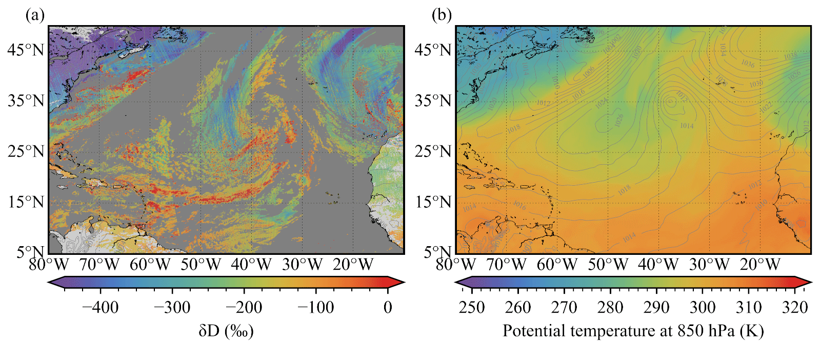
Figure 20(a) TROPOMI single-overpass δD and (b) ERA5 potential temperatures at 850 hPa at 15:00 UTC on 20 January 2020. The grey contours in all panels show ERA5 mean sea-level pressure at 15:00 UTC with a contour line distance of 2 hPa.
The analysis of successive overpasses between 18 and 20 January (Figs. 18–20) shows a rapid moistening of the originally very dry and depleted cold air mass. When it leaves the North American continent on 18 January the cold sector air has total column δD of less than −400 ‰. On 20 January, when the cold front reaches into the tropics, the δD of the cold sector is in the range −300 ‰ to −200 ‰. The dry and cold air subsiding above the boundary layer typically induces large humidity gradients near the ocean surface and consequently leads to enhanced surface evaporation fluxes that favour a rapid moistening (Aemisegger and Papritz, 2018) and continuous increase in δD of cold sector air as it travels southward. The δD in Fig. 18b shows large spatial variability in the cold sector, hinting towards different degrees of vertical mixing in different regions of the cold sector, most likely due to variations in subsidence strength. Vertical mixing between the boundary layer and the free troposphere, such as during the moistening of the cold sector, is one key process for which isotopes could provide additional information compared to total column H2O only. The latter aspect could be investigated in more detail using this dataset in combination with a numerical weather model including isotopes.
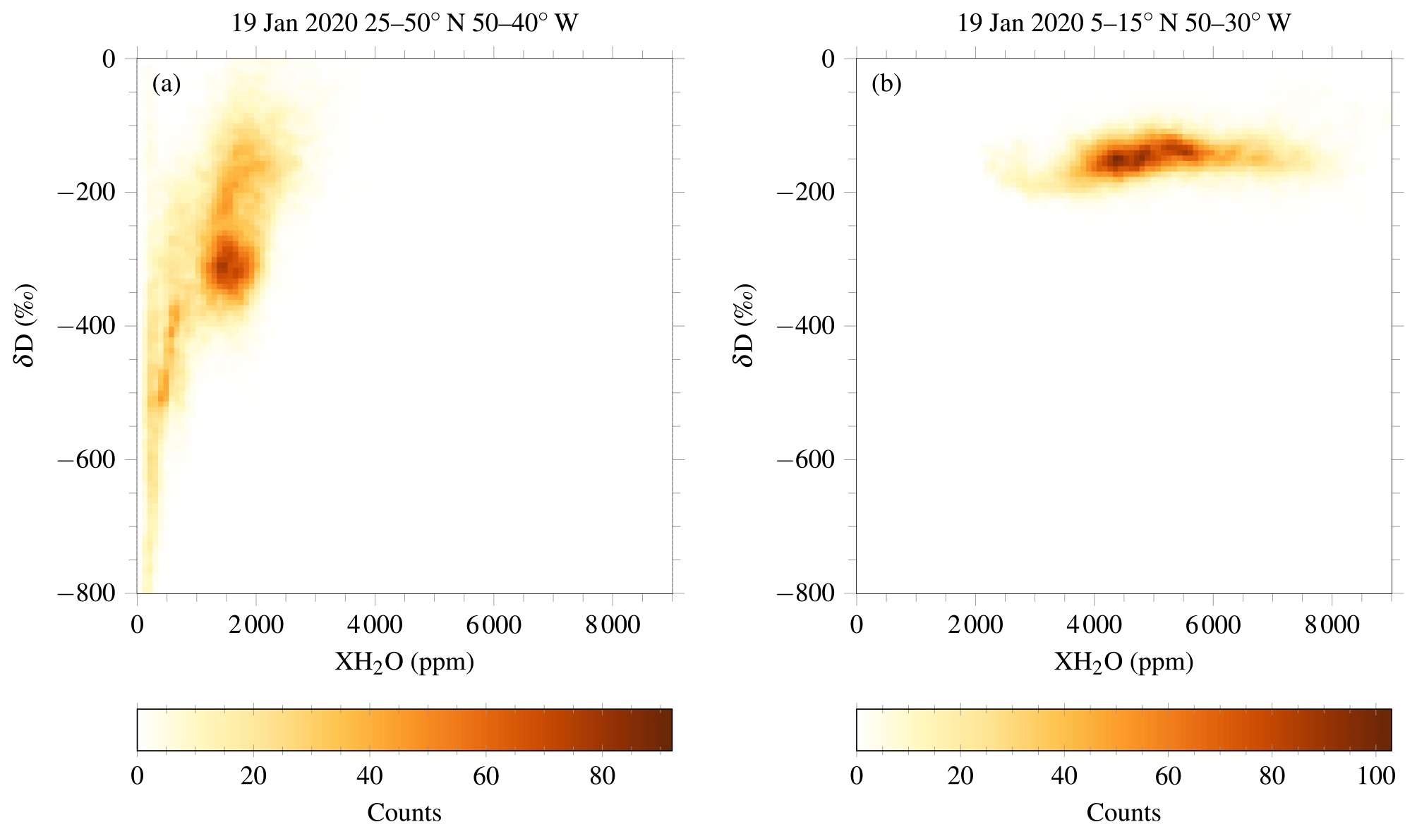
Figure 21Histograms of TROPOMI observations on 19 January 2020 (a) in the area 25–50∘ N, 50–40∘ W comprising the cold sector and (b) in the area 5–15∘ N, 50–30∘ W containing the cold front.
The large variability in δD at low total column H2O can be best observed when displaying the cold sector data in a (H2O, δD) phase space (Fig. 21), pinpointing the additional process information on boundary layer moisture export due to vertical mixing contained in δD total columns. In contrast to the cold air mass behind the cold front, the trade wind air mass in front of the cold front is associated with very high total column δD (Fig. 21b). Reduced subsidence and stronger shallow convective activity with deeper clouds are the reason for the higher δD on the warm, trade-wind side of the front (see also Aemisegger et al., 2021, for a discussion on the impact of extratropical intrusions behind cold fronts on the low-level δD signals in the tropics).
In future, comparisons of TROPOMI all-sky observations with vertical profiles from aircraft-based measurement campaigns will be helpful for identifying potentially remaining biases in very dry compared to very moist conditions. Furthermore, studies combining TROPOMI data with high-resolution numerical modelling will provide a promising data basis for studying the interaction between the moist boundary layer and the subsiding dry free tropospheric air, which is key in determining the variability in the low-level cloud cover properties.
This work presents a new dataset of H2O and HDO columns over cloudy and clear-sky scenes retrieved from TROPOMI short-wave infrared measurements. Effective cloud parameters are fitted in the spectral window 2310 to 2338 nm and taken over to the final fit of the trace gases in the spectral window 2354.0 to 2380.5 nm. Surface albedos are slightly regularised to the 1-year average of the non-scattering retrieval by Schneider et al. (2020a).
The performance of the new retrieval is similar to that of the non-scattering retrieval when comparing the same ground pixels, i.e. clear-sky scenes over land. Nevertheless, the scattering retrieval yields far more data, even for scenes classified as clear sky since the filtering is less strict. The median bias to TCCON at low-altitude stations at low and middle latitudes is for clear-sky scenes 1.3×10²¹ molec cm−2 (1.8 %) in H2O columns, 2.0×10¹⁶ molec cm−2 (−0.3 %) in HDO columns and −8 ‰ (4.6 %) in a posteriori δD, and the one for cloudy scenes is 4.7×10²¹ molec cm−2 (8.8 %) in H2O, 1.0×10¹⁸ molec cm−2 (6.5 %) in HDO columns and −20 ‰ (12 %) in δD. At high latitudes, the bias is higher (up to about 20 % in the columns and 40 ‰ in a posteriori δD) due to difficult measurement geometries with typically high solar zenith angles and low surface albedos, meaning low signal-to-noise ratios.
At high-altitude stations, the altitude difference between satellite ground pixel and FTIR instrument has to be taken into account. If not corrected for, different partial columns are compared, which leads to high biases. A correction by taking the partial column of the satellite observation above the ground station height largely reduces the biases in the H2O and HDO columns. However, the bias in a posteriori δD remains because the correction cancels out when using the same profile shapes. This bias can be eliminated by using the shielding of clouds: for cloudy scenes with cloud height similar to the station height, the bias in a posteriori δD is very low. This shows that the shielding by clouds provides information about the vertical distribution. For clear-sky observations, the bias in δD can be eliminated by using more realistic profile shapes for HDO: an experiment with an a priori profile of HDO computed from an assumed more realistic profile of δD shows a low bias in a posteriori δD after the altitude correction.
Over oceans, the retrievals are validated with aircraft profile measurements from 2018. Although the validation is hampered by a limited number of reference measurements, the available data show a good retrieval performance.
The amount of data in the new dataset is tremendously increased compared to the non-scattering retrieval by Schneider et al. (2020a). Besides more data for clear-sky scenes over land due to less strict filtering, retrievals over low clouds give new insights, particularly over oceans, where the non-scattering retrieval cannot yield data. Single overpasses yield meaningful results, which enables new case studies. As an example with cloudy scenes over the oceans, a cold air outbreak in January 2020 is shown. Retrievals from consecutive days nicely show the transport of depleted continental air from high to subtropical latitudes.
More reference measurements over oceans, either aircraft- or ship-based, will be useful for complementing the validation. Furthermore, a calibration of the TCCON HDO product would be beneficial. Moreover, a homogenisation of the ground-based data products by TCCON and MUSICA-NDACC would be valuable.
The TROPOMI HDO dataset of this study is available for download at https://tropomi.grid.surfsara.nl/hdo/ (last access: 10 March 2022, Schneider et al., 2020b). The old non-scattering data product is available at ftp://ftp.sron.nl/open-access-data-2/TROPOMI/tropomi/hdo/9_1/ (last access: 10 March 2022; Schneider et al., 2019). TCCON data are available from https://doi.org/10.14291/TCCON.GGG2014 (Total Carbon Column Observing Network Team, 2017). The individual TCCON datasets used in this study are listed in Tables 2 and 3. MUSICA data are available from https://ftp.cpc.ncep.noaa.gov/ndacc/MUSICA/ (last access: 24 March 2021; Barthlott et al., 2020), data until 2014 are also available from https://doi.org/10.5281/zenodo.48902 (Barthlott et al., 2016). Aircraft profiles from the WISPER instrument from the ORACLES 2018 campaign are available from https://doi.org/10.5281/zenodo.5748368 (Henze et al., 2022).
AS made the retrievals and performed the analysis with help from TB, JadB, AL and JL. FA performed the case study in Sect. 5.2. DN and DH provided aircraft data. RK provided TCCON data. AS prepared the manuscript with input from all the co-authors.
The contact author has declared that neither they nor their co-authors have any competing interests.
Plots and data contain modified Copernicus Sentinel data processed by SRON.
Publisher’s note: Copernicus Publications remains neutral with regard to jurisdictional claims in published maps and institutional affiliations.
This work was supported by the ESA Living Planet Fellowship project Water vapour Isotopologues from TROPOMI (WIFT). The TROPOMI data processing was carried out on the Dutch national e-infrastructure with the support of the SURF cooperative. Kimberly Strong, Justus Notholt, Debra Wunch, Christof Petri, Nicholas Deutscher, Frank Hase, Ya Té, Thorsten Warneke, Ralf Sussmann, Paul Wennberg, Isamu Morino, Laura T. Iraci, Kei Shiomi, Matthias Schneider, David Griffith, and Dave Pollard provided TCCON data. Matthias Schneider provided MUSICA-NDACC data. Two anonymous referees helped improve the manuscript with their constructive comments.
This research has been supported by the European Space Agency (grant no. 4000125587/18/I-NS).
This paper was edited by Steffen Beirle and reviewed by Christian Frankenberg and two anonymous referees.
Aemisegger, F. and Papritz, L.: A Climatology of Strong Large-Scale Ocean Evaporation Events. Part I: Identification, Global Distribution, and Associated Climate Conditions, J. Climate, 31, 7287–7312, https://doi.org/10.1175/JCLI-D-17-0591.1, 2018. a
Aemisegger, F., Vogel, R., Graf, P., Dahinden, F., Villiger, L., Jansen, F., Bony, S., Stevens, B., and Wernli, H.: How Rossby wave breaking modulates the water cycle in the North Atlantic trade wind region, Weather Clim. Dynam., 2, 281–309, https://doi.org/10.5194/wcd-2-281-2021, 2021. a
Barthlott, S., Schneider, M., Hase, F., Blumenstock, T., Mengistu Tsidu, G., Grutter de la Mora, M., Strong, K., Notholt, J., Mahieu, E., Jones, N., and Smale, D.: The ground-based MUSICA dataset: Tropospheric water vapour isotopologues (H216O, H218O, and HD16O) as obtained from NDACC/FTIR solar absorption spectra, Zenodo [data set], https://doi.org/10.5281/zenodo.48902, 2016. a
Barthlott, S., Schneider, M., Hase, F., Blumenstock, T., Kiel, M., Dubravica, D., García, O. E., Sepúlveda, E., Mengistu Tsidu, G., Takele Kenea, S., Grutter, M., Plaza-Medina, E. F., Stremme, W., Strong, K., Weaver, D., Palm, M., Warneke, T., Notholt, J., Mahieu, E., Servais, C., Jones, N., Griffith, D. W. T., Smale, D., and Robinson, J.: Tropospheric water vapour isotopologue data (H216O, H218O, and HD16O) as obtained from NDACC/FTIR solar absorption spectra, Earth Syst. Sci. Data, 9, 15–29, https://doi.org/10.5194/essd-9-15-2017, 2017. a, b
Barthlott, S., Schneider, M., Hase, F., Röhling, A. N., Blumenstock, T., Mengistu Tsidu, G., Grutter de la Mora, M., Strong, K., Notholt, J., Mahieu, E., Jones, N., and Smale, D.: The ground-based MUSICA dataset: Tropospheric water vapour isotopologues (H216O, H218O, and HD16O) as obtained from NDACC/FTIR solar absorption spectra, KIT [data set], https://ftp.cpc.ncep.noaa.gov/ndacc/MUSICA/ (last access: 24 March 2021), 2020. a
Blumenstock, T., Hase, F., Schneider, M., García, O. E., and Sepúlveda, E.: TCCON data from Izana (ES), Release GGG2014.R1, Version R1, CaltechDATA [data set], https://doi.org/10.14291/TCCON.GGG2014.IZANA01.R1, 2017. a, b
Borsdorff, T., Hasekamp, O. P., Wassmann, A., and Landgraf, J.: Insights into Tikhonov regularization: application to trace gas column retrieval and the efficient calculation of total column averaging kernels, Atmos. Meas. Tech., 7, 523–535, https://doi.org/10.5194/amt-7-523-2014, 2014. a, b, c
Craig, H.: Isotopic Variations in Meteoric Waters, Science, 133, 1702–1703, https://doi.org/10.1126/science.133.3465.1702, 1961a. a
Craig, H.: Standard for Reporting Concentrations of Deuterium and Oxygen-18 in Natural Waters, Science, 133, 1833–1834, https://doi.org/10.1126/science.133.3467.1833, 1961b. a
De Mazière, M., Thompson, A. M., Kurylo, M. J., Wild, J. D., Bernhard, G., Blumenstock, T., Braathen, G. O., Hannigan, J. W., Lambert, J.-C., Leblanc, T., McGee, T. J., Nedoluha, G., Petropavlovskikh, I., Seckmeyer, G., Simon, P. C., Steinbrecht, W., and Strahan, S. E.: The Network for the Detection of Atmospheric Composition Change (NDACC): history, status and perspectives, Atmos. Chem. Phys., 18, 4935–4964, https://doi.org/10.5194/acp-18-4935-2018, 2018. a
Deutscher, N. M., Notholt, J., Messerschmidt, J., Weinzierl, C., Warneke, T., Petri, C., and Grupe, P.: TCCON data from Bialystok (PL), Release GGG2014.R2, Version R2, CaltechDATA [data set], https://doi.org/10.14291/TCCON.GGG2014.BIALYSTOK01.R2, 2019. a
Fletcher, J. K., Mason, S., and Jakob, C.: A Climatology of Clouds in Marine Cold Air Outbreaks in Both Hemispheres, J. Climate, 29, 6677–6692, https://doi.org/10.1175/JCLI-D-15-0783.1, 2016. a
Gordon, I., Rothman, L., Hill, C., Kochanov, R., Tan, Y., Bernath, P., Birk, M., Boudon, V., Campargue, A., Chance, K., Drouin, B., Flaud, J.-M., Gamache, R., Hodges, J., Jacquemart, D., Perevalov, V., Perrin, A., Shine, K., Smith, M.-A., Tennyson, J., Toon, G., Tran, H., Tyuterev, V., Barbe, A., Császár, A., Devi, V., Furtenbacher, T., Harrison, J., Hartmann, J.-M., Jolly, A., Johnson, T., Karman, T., Kleiner, I., Kyuberis, A., Loos, J., Lyulin, O., Massie, S., Mikhailenko, S., Moazzen-Ahmadi, N., Müller, H., Naumenko, O., Nikitin, A., Polyansky, O., Rey, M., Rotger, M., Sharpe, S., Sung, K., Starikova, E., Tashkun, S., Auwera, J. V., Wagner, G., Wilzewski, J., Wcislo, P., Yu, S., and Zak, E.: The HITRAN2016 molecular spectroscopic database, J. Quant. Spectrosc. Ra., 203, 3–69, https://doi.org/10.1016/j.jqsrt.2017.06.038, 2017. a
Griffith, D. W., Velazco, V. A., Deutscher, N. M., Paton-Walsh, C., Jones, N. B., Wilson, S. R., Macatangay, R. C., Kettlewell, G. C., Buchholz, R. R., and Riggenbach, M. O.: TCCON data from Wollongong (AU), Release GGG2014.R0, Version GGG2014.R0, CaltechDATA [data set], https://doi.org/10.14291/TCCON.GGG2014.WOLLONGONG01.R0/1149291, 2014. a, b
Hagemann, R., Nief, G., and Roth, E.: Absolute isotopic scale for deuterium analysis of natural waters. Absolute DH ratio for SMOW, Tellus, 22, 712–715, https://doi.org/10.3402/tellusa.v22i6.10278, 1970. a
Hase, F., Blumenstock, T., Dohe, S., Groß, J., and Kiel, M.: TCCON data from Karlsruhe (DE), Release GGG2014.R1, Version GGG2014.R1, CaltechDATA [data set], https://doi.org/10.14291/TCCON.GGG2014.KARLSRUHE01.R1/1182416, 2015. a, b
Henze, D., Noone, D., and Toohey, D.: Aircraft measurements of water vapor heavy isotope ratios in the marine boundary layer and lower troposphere during ORACLES, Earth Syst. Sci. Data Discuss. [preprint], https://doi.org/10.5194/essd-2021-238, in review, 2021. a
Henze, D., Noone, D., and Toohey, D.: Aircraft profiles of stable isotope ratios in atmospheric total and condensed water from the NASA ORACLES mission (1.0), Zenodo [data set], https://doi.org/10.5281/zenodo.5748368, 2022. a
Herbin, H., Hurtmans, D., Clerbaux, C., Clarisse, L., and Coheur, P.-F.: H216O and HDO measurements with IASI/MetOp, Atmos. Chem. Phys., 9, 9433–9447, https://doi.org/10.5194/acp-9-9433-2009, 2009. a
Iraci, L. T., Podolske, J. R., Hillyard, P. W., Roehl, C., Wennberg, P. O., Blavier, J.-F., Landeros, J., Allen, N., Wunch, D., Zavaleta, J., Quigley, E., Osterman, G. B., Albertson, R., Dunwoody, K., and Boyden, H.: TCCON data from Edwards (US), Release GGG2014.R1, Version GGG2014.R1, CaltechDATA [data set], https://doi.org/10.14291/TCCON.GGG2014.EDWARDS01.R1/1255068, 2016. a
Kawakami, S., Ohyama, H., Arai, K., Okumura, H., Taura, C., Fukamachi, T., and Sakashita, M.: TCCON data from Saga (JP), Release GGG2014.R0, Version GGG2014.R0, CaltechDATA [data set], https://doi.org/10.14291/TCCON.GGG2014.SAGA01.R0/1149283, 2014. a
Kivi, R., Heikkinen, P., and Kyrö, E.: TCCON data from Sodankylä (FI), Release GGG2014.R0, CaltechDATA [data set], https://doi.org/10.14291/tccon.ggg2014.sodankyla01.R0/1149280, 2014. a
Krol, M., Houweling, S., Bregman, B., van den Broek, M., Segers, A., van Velthoven, P., Peters, W., Dentener, F., and Bergamaschi, P.: The two-way nested global chemistry-transport zoom model TM5: algorithm and applications, Atmos. Chem. Phys., 5, 417–432, https://doi.org/10.5194/acp-5-417-2005, 2005. a
Lacour, J.-L., Risi, C., Clarisse, L., Bony, S., Hurtmans, D., Clerbaux, C., and Coheur, P.-F.: Mid-tropospheric δD observations from IASI/MetOp at high spatial and temporal resolution, Atmos. Chem. Phys., 12, 10817–10832, https://doi.org/10.5194/acp-12-10817-2012, 2012. a
Landgraf, J., aan de Brugh, J., Scheepmaker, R., Borsdorff, T., Hu, H., Houweling, S., Butz, A., Aben, I., and Hasekamp, O.: Carbon monoxide total column retrievals from TROPOMI shortwave infrared measurements, Atmos. Meas. Tech., 9, 4955–4975, https://doi.org/10.5194/amt-9-4955-2016, 2016. a, b
Morino, I., Matsuzaki, T., and Horikawa, M.: TCCON data from Tsukuba (JP), 125HR, Release GGG2014.R2, Version R2, CaltechDATA [data set], https://doi.org/10.14291/TCCON.GGG2014.TSUKUBA02.R2, 2018a. a
Morino, I., Velazco, V. A., Hori, A., Uchino, O., and Griffith, D. W.: TCCON data from Burgos, Ilocos Norte (PH), Release GGG2014.R0, Version GGG2014.R0, CaltechDATA [data set], https://doi.org/10.14291/TCCON.GGG2014.BURGOS01.R0, 2018b. a
Morino, I., Yokozeki, N., Matsuzaki, T., and Horikawa, M.: TCCON data from Rikubetsu (JP), Release GGG2014.R2, Version R2, CaltechDATA [data set], https://doi.org/10.14291/TCCON.GGG2014.RIKUBETSU01.R2, 2018c. a
Notholt, J., Petri, C., Warneke, T., Deutscher, N. M., Palm, M., Buschmann, M., Weinzierl, C., Macatangay, R. C., and Grupe, P.: TCCON data from Bremen (DE), Release GGG2014.R1, Version GGG2014.R0, CaltechDATA [data set], https://doi.org/10.14291/TCCON.GGG2014.BREMEN01.R0/1149275, 2019a. a, b
Notholt, J., Warneke, T., Petri, C., Deutscher, N. M., Weinzierl, C., Palm, M., and Buschmann, M.: TCCON data from Ny Ålesund, Spitsbergen (NO), Release GGG2014.R1, Version R1, CaltechDATA [data set], https://doi.org/10.14291/TCCON.GGG2014.NYALESUND01.R1, 2019b. a, b
Pollard, D. F., Robinson, J., and Shiona, H.: TCCON data from Lauder (NZ), Release GGG2014.R0, Version GGG2014.R0, CaltechDATA [data set], https://doi.org/10.14291/TCCON.GGG2014.LAUDER03.R0, 2019. a
Rast, M., Johannessen, J., and Mauser, W.: Review of Understanding of Earth's Hydrological Cycle: Observations, Theory and Modelling, Surv. Geophys., 35, 491–513, https://doi.org/10.1007/s10712-014-9279-x, 2014. a
Redemann, J., Wood, R., Zuidema, P., Doherty, S. J., Luna, B., LeBlanc, S. E., Diamond, M. S., Shinozuka, Y., Chang, I. Y., Ueyama, R., Pfister, L., Ryoo, J.-M., Dobracki, A. N., da Silva, A. M., Longo, K. M., Kacenelenbogen, M. S., Flynn, C. J., Pistone, K., Knox, N. M., Piketh, S. J., Haywood, J. M., Formenti, P., Mallet, M., Stier, P., Ackerman, A. S., Bauer, S. E., Fridlind, A. M., Carmichael, G. R., Saide, P. E., Ferrada, G. A., Howell, S. G., Freitag, S., Cairns, B., Holben, B. N., Knobelspiesse, K. D., Tanelli, S., L'Ecuyer, T. S., Dzambo, A. M., Sy, O. O., McFarquhar, G. M., Poellot, M. R., Gupta, S., O'Brien, J. R., Nenes, A., Kacarab, M., Wong, J. P. S., Small-Griswold, J. D., Thornhill, K. L., Noone, D., Podolske, J. R., Schmidt, K. S., Pilewskie, P., Chen, H., Cochrane, S. P., Sedlacek, A. J., Lang, T. J., Stith, E., Segal-Rozenhaimer, M., Ferrare, R. A., Burton, S. P., Hostetler, C. A., Diner, D. J., Seidel, F. C., Platnick, S. E., Myers, J. S., Meyer, K. G., Spangenberg, D. A., Maring, H., and Gao, L.: An overview of the ORACLES (ObseRvations of Aerosols above CLouds and their intEractionS) project: aerosol–cloud–radiation interactions in the southeast Atlantic basin, Atmos. Chem. Phys., 21, 1507–1563, https://doi.org/10.5194/acp-21-1507-2021, 2021. a
Scheepmaker, R. A., aan de Brugh, J., Hu, H., Borsdorff, T., Frankenberg, C., Risi, C., Hasekamp, O., Aben, I., and Landgraf, J.: HDO and H2O total column retrievals from TROPOMI shortwave infrared measurements, Atmos. Meas. Tech., 9, 3921–3937, https://doi.org/10.5194/amt-9-3921-2016, 2016. a, b, c
Schneider, A., Borsdorff, T., aan de Brugh, J., Hu, H., and Landgraf, J.: A full-mission data set of H2O and HDO columns from SCIAMACHY 2.3 µm reflectance measurements, Atmos. Meas. Tech., 11, 3339–3350, https://doi.org/10.5194/amt-11-3339-2018, 2018. a
Schneider, A., Borsdorff, T., aan de Brugh, J., and Landgraf, J.: TROPOMI H2O/HDO column dataset for clear-sky scenes, SRON, ftp://ftp.sron.nl/open-access-data-2/TROPOMI/tropomi/hdo/9_1/ (last access: 10 March 2022), 2019. a
Schneider, A., Borsdorff, T., aan de Brugh, J., Aemisegger, F., Feist, D. G., Kivi, R., Hase, F., Schneider, M., and Landgraf, J.: First data set of H2O/HDO columns from the Tropospheric Monitoring Instrument (TROPOMI), Atmos. Meas. Tech., 13, 85–100, https://doi.org/10.5194/amt-13-85-2020, 2020a. a, b, c, d, e, f, g, h, i, j, k, l, m, n, o, p, q
Schneider, A., Borsdorff, T., aan de Brugh, J., Lorente, A., and Landgraf, J.: TROPOMI H2O/HDO column dataset for clear-sky and cloudy scenes, SRON, https://tropomi.grid.surfsara.nl/hdo/ (last access: 10 March 2022), 2020b. a
Schneider, M. and Hase, F.: Optimal estimation of tropospheric H2O and δD with IASI/METOP, Atmos. Chem. Phys., 11, 11207–11220, https://doi.org/10.5194/acp-11-11207-2011, 2011. a
Schneider, M., Wiegele, A., Barthlott, S., González, Y., Christner, E., Dyroff, C., García, O. E., Hase, F., Blumenstock, T., Sepúlveda, E., Mengistu Tsidu, G., Takele Kenea, S., Rodríguez, S., and Andrey, J.: Accomplishments of the MUSICA project to provide accurate, long-term, global and high-resolution observations of tropospheric {H2O,δD} pairs – a review, Atmos. Meas. Tech., 9, 2845–2875, https://doi.org/10.5194/amt-9-2845-2016, 2016. a, b
Sherlock, V., Connor, B., Robinson, J., Shiona, H., Smale, D., and Pollard, D. F.: TCCON data from Lauder (NZ), 125HR, Release GGG2014.R0, Version GGG2014.R0, CaltechDATA [data set], https://doi.org/10.14291/TCCON.GGG2014.LAUDER02.R0/1149298, 2014. a, b
Stevens, B. and Bony, S.: What Are Climate Models Missing?, Science, 340, 1053–1054, https://doi.org/10.1126/science.1237554, 2013. a
Strong, K., Roche, S., Franklin, J. E., Mendonca, J., Lutsch, E., Weaver, D., Fogal, P. F., Drummond, J. R., Batchelor, R., and Lindenmaier, R.: TCCON data from Eureka (CA), Release GGG2014.R3, Version R3, CaltechDATA [data set], https://doi.org/10.14291/TCCON.GGG2014.EUREKA01.R3, 2019. a, b
Sussmann, R. and Rettinger, M.: TCCON data from Garmisch (DE), Release GGG2014.R2, Version R2, CaltechDATA [data set], https://doi.org/10.14291/TCCON.GGG2014.GARMISCH01.R2, 2018a. a
Sussmann, R. and Rettinger, M.: TCCON data from Zugspitze (DE), Release GGG2014.R1, Version R1, CaltechDATA [data set], https://doi.org/10.14291/TCCON.GGG2014.ZUGSPITZE01.R1, 2018b. a
Té, Y., Jeseck, P., and Janssen, C.: TCCON data from Paris (FR), Release GGG2014.R0, Version GGG2014.R0, CaltechDATA [data set], https://doi.org/10.14291/TCCON.GGG2014.PARIS01.R0/1149279, 2014. a
Thurnherr, I., Hartmuth, K., Jansing, L., Gehring, J., Boettcher, M., Gorodetskaya, I., Werner, M., Wernli, H., and Aemisegger, F.: The role of air–sea fluxes for the water vapour isotope signals in the cold and warm sectors of extratropical cyclones over the Southern Ocean, Weather Clim. Dynam., 2, 331–357, https://doi.org/10.5194/wcd-2-331-2021, 2021. a
Total Carbon Column Observing Network (TCCON) Team: 2014 TCCON Data Release, Version GGG2014, CaltechDATA [data set], https://doi.org/10.14291/TCCON.GGG2014, 2017. a
Veefkind, J. P., Aben, I., McMullan, K., Förster, H., de Vries, J., Otter, G., Claas, J., Eskes, H. J., de Haan, J. F., Kleipool, Q., van Weele, M., Hasekamp, O., Hoogeveen, R., Landgraf, J., Snel, R., Tol, P., Ingmann, P., Voors, R., Kruizinga, B., Vink, R., Visser, H., and Levelt, P. F.: TROPOMI on the ESA Sentinel-5 Precursor: A GMES mission for global observations of the atmospheric composition for climate, air quality and ozone layer applications, Remote Sens. Environ., 120, 70–83, https://doi.org/10.1016/j.rse.2011.09.027, 2012. a
Warneke, T., Messerschmidt, J., Notholt, J., Weinzierl, C., Deutscher, N. M., Petri, C., and Grupe, P.: TCCON data from Orléans (FR), Release GGG2014.R1, Version R1, CaltechDATA [data set], https://doi.org/10.14291/TCCON.GGG2014.ORLEANS01.R1, 2019. a
Wennberg, P. O., Wunch, D., Roehl, C. M., Blavier, J.-F., Toon, G. C., and Allen, N. T.: TCCON data from Caltech (US), Release GGG2014.R1, Version GGG2014.R1, CaltechDATA [data set], https://doi.org/10.14291/TCCON.GGG2014.PASADENA01.R1/1182415, 2015. a
Wennberg, P. O., Roehl, C. M., Blavier, J.-F., Wunch, D., and Allen, N. T.: TCCON data from Jet Propulsion Laboratory (US), 2011, Release GGG2014.R1, Version GGG2014.R1, CaltechDATA [data set], https://doi.org/10.14291/TCCON.GGG2014.JPL02.R1/1330096, 2016a. a
Wennberg, P. O., Wunch, D., Roehl, C. M., Blavier, J.-F., Toon, G. C., and Allen, N. T.: TCCON data from Lamont (US), Release GGG2014.R1, Version GGG2014.R1, CaltechDATA [data set], https://doi.org/10.14291/TCCON.GGG2014.LAMONT01.R1/1255070, 2016b. a
Wennberg, P. O., Roehl, C. M., Wunch, D., Toon, G. C., Blavier, J.-F., Washenfelder, R., Keppel-Aleks, G., Allen, N. T., and Ayers, J.: TCCON data from Park Falls (US), Release GGG2014.R1, Version GGG2014.R1, CaltechDATA [data set], https://doi.org/10.14291/TCCON.GGG2014.PARKFALLS01.R1, 2017. a
Worden, J., Kulawik, S., Frankenberg, C., Payne, V., Bowman, K., Cady-Peirara, K., Wecht, K., Lee, J.-E., and Noone, D.: Profiles of CH4, HDO, H2O, and N2O with improved lower tropospheric vertical resolution from Aura TES radiances, Atmos. Meas. Tech., 5, 397–411, https://doi.org/10.5194/amt-5-397-2012, 2012. a
Worden, J. R., Kulawik, S. S., Fu, D., Payne, V. H., Lipton, A. E., Polonsky, I., He, Y., Cady-Pereira, K., Moncet, J.-L., Herman, R. L., Irion, F. W., and Bowman, K. W.: Characterization and evaluation of AIRS-based estimates of the deuterium content of water vapor, Atmos. Meas. Tech., 12, 2331–2339, https://doi.org/10.5194/amt-12-2331-2019, 2019. a
Wunch, D., Toon, G. C., Blavier, J.-F. L., Washenfelder, R. A., Notholt, J., Connor, B. J., Griffith, D. W. T., Sherlock, V., and Wennberg, P. O.: The Total Carbon Column Observing Network, Philos. T. R. Soc. A, 369, 2087–2112, https://doi.org/10.1098/rsta.2010.0240, 2011. a
Wunch, D., Toon, G. C., Sherlock, V., Deutscher, N. M., Liu, C., Feist, D. G., and Wennberg, P. O.: Documentation for the 2014 TCCON Data Release, CaltechDATA, https://doi.org/10.14291/TCCON.GGG2014.DOCUMENTATION.R0/1221662, 2015. a
Wunch, D., Mendonca, J., Colebatch, O., Allen, N. T., Blavier, J.-F., Roche, S., Hedelius, J., Neufeld, G., Springett, S., Worthy, D., Kessler, R., and Strong, K.: TCCON data from East Trout Lake, SK (CA), Release GGG2014.R1, Version R1, CaltechDATA [data set], https://doi.org/10.14291/TCCON.GGG2014.EASTTROUTLAKE01.R1, 2018. a
Zdunkowski, W. G., Welch, R. M., and Korb, G.: An Investigation of the Structure of Typical Two-stream-methods for the Calculation of Solar Fluxes and Heating Rates in Clouds, Contrib. Atmos. Phys., 53, 147–166, 1980. a