Satellite data validation: a parametrization of the natural variability of atmospheric mixing ratios

High-resolution model data are used to estimate the statistically typical mixing ratio variabilities of trace species as a function of distance and time separation. These estimates can be used to explain the fact that some of the differences between observations made with different observing systems are due to the less-than-perfect co-location of the measurements. The variability function is approximated by a two-parameter regression function, and lookup tables of the natural variability values as a function of distance separation and time separation are provided. In addition, a reparametrization of the variability values as a function of latitudinal gradients is proposed, and the seasonal independence of the linear approximation of such a function is demonstrated.

1 Introduction

This paper tackles a problem that typically arises when remotely sensed data from different instruments are compared within the framework of validation studies. In quantitative validation, the common approach is to calculate differences between pairs of measurements of the same air mass from the two instruments under comparison. With the aid of χ² statistics, it is tested if the observed differences can be explained by the estimated error of the differences (Rodgers and Connor, 2003). The estimated error of the differences includes measurement noise as well as parameter and model errors, as far as those coming from different instruments are uncorrelated (von Clarmann, 2006). Furthermore, the different impact of prior information on the result has to be considered. However, the differences will often be too large to be explained by the combined error budget of the measurements under comparison. The reason for this is that the instruments typically do not sound exactly the same air mass. Spatial and temporal mismatch of the measurements as well as natural variability of the measured state variable contribute to the observed differences. This source of differences is only quantified in validation papers in a few exceptional cases (see, e.g., Sheese et al., 2021, for an example where models were used to quantify the related effect of ozone variability). Instead, natural variability is often used as a universal excuse to defend measurements if validation studies suggest that the related retrieval errors are underestimated.

In this study, we present a user-friendly tool to provide quantitative estimates of the component of the observation differences that can be attributed to the spatial and temporal mismatch and natural variability. The underlying method is based on highly resolved model fields of temperature and mixing ratios of trace species, as described in Sect. 2. These model fields were smoothed according to the horizontal resolution of the instruments whose precision was to be validated; in this study, we have chosen the Michelson Interferometer for Passive Atmospheric Sounding (MIPAS; Fischer et al., 2008) as an example. From these smoothed fields, the typical variabilities are evaluated as a function of spatial and temporal mismatch (Sect. 3). In order to avoid unnecessarily high data traffic and to reduce the impact of model imperfections on the calculated fields as much as possible, parametrizations of these dependencies (for different trace gases, altitudes and latitude bins) are developed by prescribing a particular shape to the natural variability function, which arises from the general theory of random functions with stationary increments (Sect. 4) and is confirmed by calculations using model data. A reparametrization is developed to improve the validity of the inductive generalization towards other gases and seasons (Sect. 5). Instructions on how to use this reparametrization are given in Sect. 6. The adequacy of our suggested method is critically discussed in Sect. 7, and final recommendations are given in Sect. 8.

2 Model data

The model fields used in this study came from two models.

2.1 BASCOE (Belgian Assimilation System for Chemical ObsErvations)

The main set of model fields has been produced by the Belgian Assimilation System for Chemical ObsErvations (BASCOE; Errera et al., 2008). While generally used in the context of stratospheric chemical data assimilation (e.g., Errera et al., 2019), the chemistry transport model (CTM) of the system has also been used to study the evolution of the stratospheric composition (Chabrillat et al., 2018; Prignon et al., 2019; Minganti et al., 2020). Here, BASCOE was run for the period from 25 September to 1 October 2008, and wind and temperature were taken from the ERA-Interim reanalysis (Dee et al., 2011). The model was run on a $\mathrm{1}{}^{\circ }\times \mathrm{1}{}^{\circ }$ horizontal grid using the native 60 vertical levels of ERA-Interim (from the surface to 0.1 hPa) and a time step of 30 min. Hourly global fields of 28 relevant trace gases¹ were used for this study.

2.2 WACCM6 (Whole Atmosphere Community Climate Model 6)

The auxiliary set of model fields used came from the Whole Atmosphere Community Climate Model 6 (WACCM6), which is the atmospheric component of the Community Earth System Model, version 2 (CESM2; Danabasoglu et al., 2019; Emmons et al., 2019; Gettelman et al., 2019; Tilmes et al., 2019), run at the Atmospheric Chemistry Observations and Modelling Laboratory of the National Center of Atmospheric Research (UCAR/NCAR/ACOM). The model has a horizontal resolution of $\mathrm{0.9}{}^{\circ }\times \mathrm{1.25}{}^{\circ }$ with 88 vertical hybrid sigma-pressure levels and is run using specified dynamics, with nudging of temperature, and $\mathit{U}/\mathit{V}$ winds from the NASA Goddard Earth Observing System, version 5 (GEOS-5), forecast model. The model simulations contain the fields of three species (O₃, H₂O and NO) for 4 weeks in the year 2020, one in each season. The data were regridded on the same fixed height grid with a 1 km step using the fields of geopotential height and temperature provided with the data.

3 Variabilities

3.1 Structure functions

Let X be a random variable defined by the amount of the target trace gas in a given infinitely small air parcel, centered around a point in the atmosphere at a given moment in time and reported as a volume mixing ratio (VMR). The amount of the trace gas at any point in the atmosphere at a fixed time (or at any moment in time at a fixed point in the atmosphere) can be viewed as a state of a one-dimensional random process X(t), where t parameterizes the distance from an initial point (or the time elapsed from an initial moment). This random process is nonstationary, as its statistical characteristics can change with t. The increments $X(t+\mathit{\tau })-X\left(t\right)$ of the process X(t) represent the change in the amount of the trace gas with distance (or over time). Based on the literature, we assume that, in a given sufficiently narrow latitude band, at a fixed altitude and in a given season, the distribution of the differences $X(t+\mathit{\tau })-X\left(t\right)$ does not depend on t, which means that X(t) is a process with stationary increments. The basic characteristics of real-valued random process with stationary increments are the mean value of the increment $E\left[X(t+\mathit{\tau })-X\left(t\right)\right]$ and the correlation function of the increment

$$\begin{array}{}\text{(1)}& D\left(\mathit{\tau }\right)=E\left|X\right(t+\mathit{\tau })-X(t){|}^{\mathrm{2}},\end{array}$$

also called the “structure function” of the process X(t) (Yaglom, 1986, chap. 23). In our case, as $E\left[X(t+\mathit{\tau })-X\left(t\right)\right]=\mathrm{0}$,

$$\begin{array}{}\text{(2)}& \begin{array}{rl}D\left(\mathit{\tau }\right)& =E\left|X\right(t+\mathit{\tau })-X(t){|}^{\mathrm{2}}\\ & ={\mathit{\sigma }}^{\mathrm{2}}\left(\right|X(t+\mathit{\tau })-X\left(t\right)\left|\right)+\left(E\right|X(t+\mathit{\tau })-X\left(t\right)|{)}^{\mathrm{2}}\\ & ={\mathit{\sigma }}^{\mathrm{2}}\left(\right|X(t+\mathit{\tau })-X\left(t\right)\left|\right).\end{array}\end{array}$$

The natural variability of a trace gas is the square root of the structure function of the process X(t):

$$\begin{array}{}\text{(3)}& \sqrt{D\left(\mathit{\tau }\right)}=\mathit{\sigma }\left(\right|X(t+\mathit{\tau })-X\left(t\right)\left|\right).\end{array}$$

This provides the formal link between the intuitive definition of the natural variability, as the variability of differences, and the mathematical machinery of random processes with stationary increments, which is widely used in studying the processes at smaller spatiotemporal scales, for example, in the theory of atmospheric turbulence. This link will allow us to draw conclusions about the nature of the process X(t) based on the shape of the obtained statistics and will justify the choice of the form of the regression function for the natural variability of trace gases. The next section explains how the estimation of $\sqrt{D}$ is done out of model fields.

3.2 Estimation of variabilities

In order to obtain a statistic of the variability of differences, the model fields were first transformed from their native hybrid sigma-pressure vertical grid to a fixed 1 km step geometrical height grid. For this, the geopotential height for each model knot was restored and transformed into geometrical height using the temperature values from the model, which allowed the interpolation of the profiles on a fixed altitude grid. Second, the model fields were smoothed according to the horizontal resolution of the instruments whose precision was to be validated. We have chosen the MIPAS instrument as an example. Its cross-track resolution roughly corresponds to an east–west resolution and is defined by the width of the instantaneous field of view at the tangent point, which is 30 km. The along-track smearing, which roughly corresponds to a north–south horizontal resolution, is roughly 200 km on average (von Clarmann et al., 2009). This smoothing operation does not influence the shape of the obtained curves, but it does reduce the obtained variability values by around 0.05 %. No vertical smoothing is applied, as vertical smoothing is typically considered in an explicit manner in validation via the averaging kernels. These smoothed fields are the basis for the statistics of the horizontal and temporal variability of the atmospheric state.

3.2.1 Horizontal variability

We take the model data within a fixed 10^∘ latitude bin and at a fixed height; as each of the five model data sets used (one from BASCOE and four from WACCM6) covers only 1 week, there is no need to fix a season. For all possible pairs of points in the obtained subset, the normalized differences of the VMR of the target trace species within a predefined radius of 1500 km are calculated:

$$\begin{array}{}\text{(4)}& {\displaystyle \frac{\text{VMR}({\text{location}}_{\mathrm{1}},t)-\text{VMR}({\text{location}}_{\mathrm{2}},t)}{{\text{VMR}}_{\mathrm{mean}}}},\end{array}$$

with VMR_mean being the mean VMR values of the target trace gas in the chosen latitude band at the chosen height. The constant time index t indicates that only differences where the subtractor and the subtrahend refer to the same time are considered. These differences are binned according to their horizontal separation distance. The following bins were used: 0–100 km between the two points, 100–200 km between the two points, etc. We calculate the standard deviation of the sample of these normalized differences, which provides us with an estimator of the natural variability of the target trace gas as a function of distance separation. The obtained estimation of the natural variability of ozone at 35 km altitude as a function of distance is shown in Fig. 1a. The fast growth of the variability for separation distances over 1000 km at high northern latitudes reflects that, in many pairs of corresponding samples, one point lies inside the polar vortex whereas the other lies outside. Note also that the calculated variability values for the distances from 0 to 100 km are zero for the tropical latitudes (yellow curves in Fig. 1) and present a peak at subtropical latitudes (clear orange and clear green curves in Fig. 1). This is due to the models' resolutions: the samples for 100 km distance separation are empty or very small at low latitudes. Therefore, the 100 km point will not be taken into account in the calculation of regression coefficients at these latitudes.

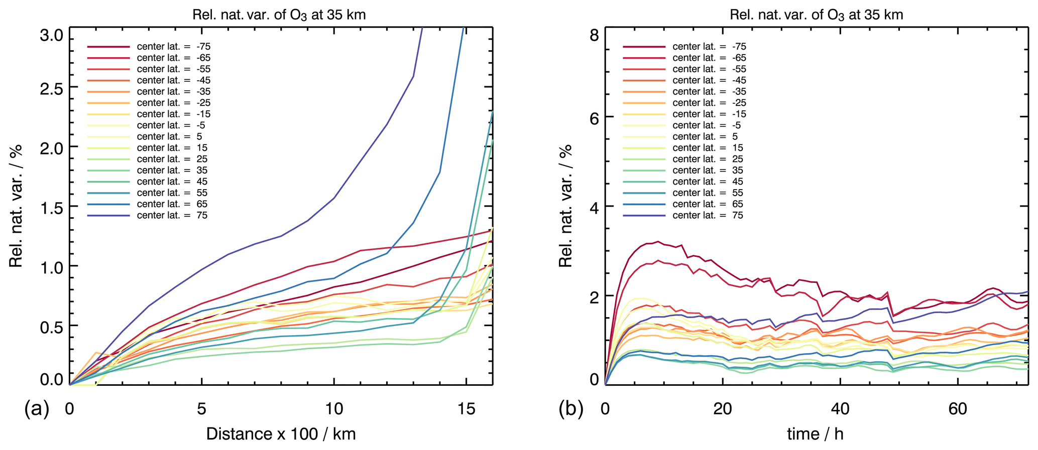
Figure 1 (a) Natural variability of O₃ at 35 km altitude as a function of horizontal distance in the BASCOE model. (b) Natural variability of O₃ at 35 km altitude as a function of time separation in the BASCOE model.

3.2.2 Temporal variability

In a similar fashion to that described above, for all possible pairs of data points for the entire data set, the differences of the VMR of the target trace gas within a predefined time period of 72 h are calculated for each latitude band and height:

$$\begin{array}{}\text{(5)}& {\displaystyle \frac{\text{VMR}(\text{location},t_{\mathrm{1}})-\text{VMR}(\text{location},t_{\mathrm{2}})}{{\text{VMR}}_{\mathrm{mean}}}}.\end{array}$$

The constant location index “location” indicates that differences are only considered when the subtractor and the subtrahend refer to the same location. These differences are sorted according to their time lag. Similar to the horizontal variability, for each time lag, the differences are normalized by the mean VMR within given latitude band at given altitude, and the standard deviation of the sample of normalized differences is then calculated. This quantity is the estimator of the natural variability of the target species as a function of time separation, and we note it as σ_rel,time; its values for ozone at 35 km altitude are shown in Fig. 1b. As for most satellite validation exercises, time separation within co-location criteria stays within 5 h, and we made the choice to restrain our analysis to a maximum time separation lag of 5 h.

3.3 Combination of horizontal and temporal variability

Despite the fact that advection can admittedly cause correlations between horizontal and temporal components of the variability, at the scales considered here, we assume that horizontal and temporal variations of the atmospheric state are uncorrelated. Tests using a statistic of combined horizontal and temporal differences of the type

$$\begin{array}{}\text{(6)}& \text{VMR}({\text{location}}_{\mathrm{1}},t_{\mathrm{1}})-\text{VMR}({\text{location}}_{\mathrm{2}},t_{\mathrm{2}})\end{array}$$

have shown that, at the scales considered here, the error due to the neglect of correlations is below 0.1 % and, thus, not usually worth an additional effort. In our analysis, we offer independent parametrizations for each of them, which are recommended to be combined with their quadratic sum; we also provide a software that performs this summation for a reparametrization of these quantities on latitudinal gradients, and this software is described in the Sect. 6.

We do not consider the vertical variability in the present work, and the fields are calculated independently for each altitude level. Note that atmospheric variability as a function of distance and time separation could be approximately represented by a two-dimensional random process; however, this is outside the scope of this paper: our choice is to treat the distance and time mismatch dependences separately, as this is what a typical validation exercise does.

4 Parametrization

4.1 Motivation

The goal of the present work is to provide the community with information on the natural variability of trace gas mixing ratios as a function of distance and time separation. This information is meant to be used in the context of validation studies. Instead of providing the entire variability data set, we consider the use of a simple and easy-to-use parametrization as more adequate. The reasons for this are as follows: (1) the use of parametrizations avoids a considerable amount of data traffic, (2) the fine structure of the fields reflects the actual conditions of the days actually covered by the model run rather than the general behavior of the atmosphere, and (3) our parametrization using continuous regression functions allows for easy interpolation.

4.2 The regression function

In view of the shape of the curves produced from model data (Sect. 3.2.2 and 3.2.1), the natural variability function can be parameterized in the form D(τ)=Aτ^γ, where A>0, and $\mathrm{0}<\mathit{\gamma }<\mathrm{1}$. An interesting side conclusion that can be made from the obtained shape of the structure function of X(t) is that the process of the atmospheric variability (horizontal and temporal variability) of mixing ratios is self-similar: the form of its structure function D(τ)=Aτ^γ is invariant under a group of similarity transformations, t→ht and X→a(h)X (Kolmogorov, 1940; Yaglom, 1986); in other words, no characteristic scale can be associated with their structure function.

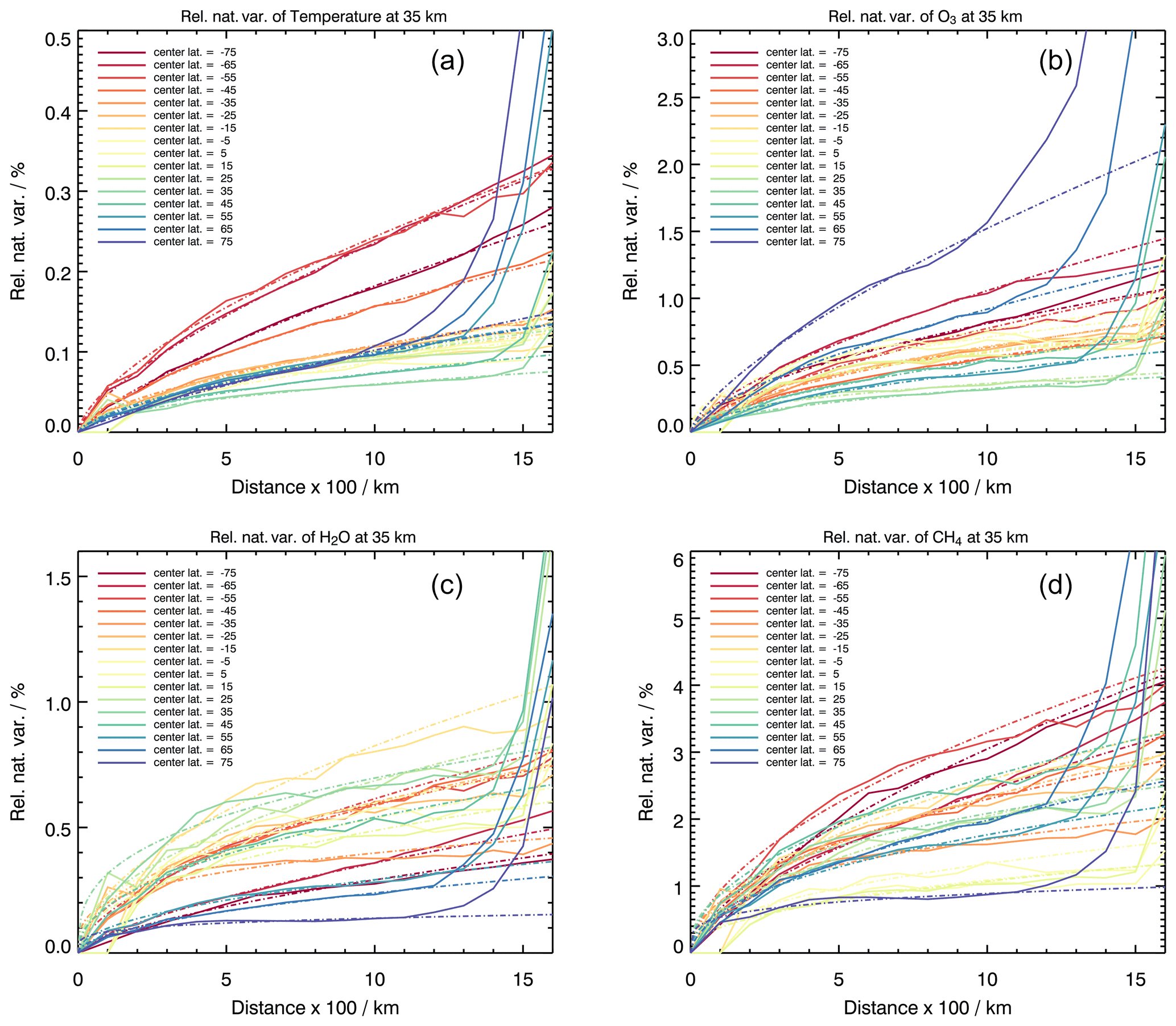
Figure 2 Natural variability as a function of horizontal distance for (a) temperature, (b) O₃, (c) H₂O and (d) CH₄ in the BASCOE model (solid lines) and the proposed parametrization (dashed lines) in different latitude bins.

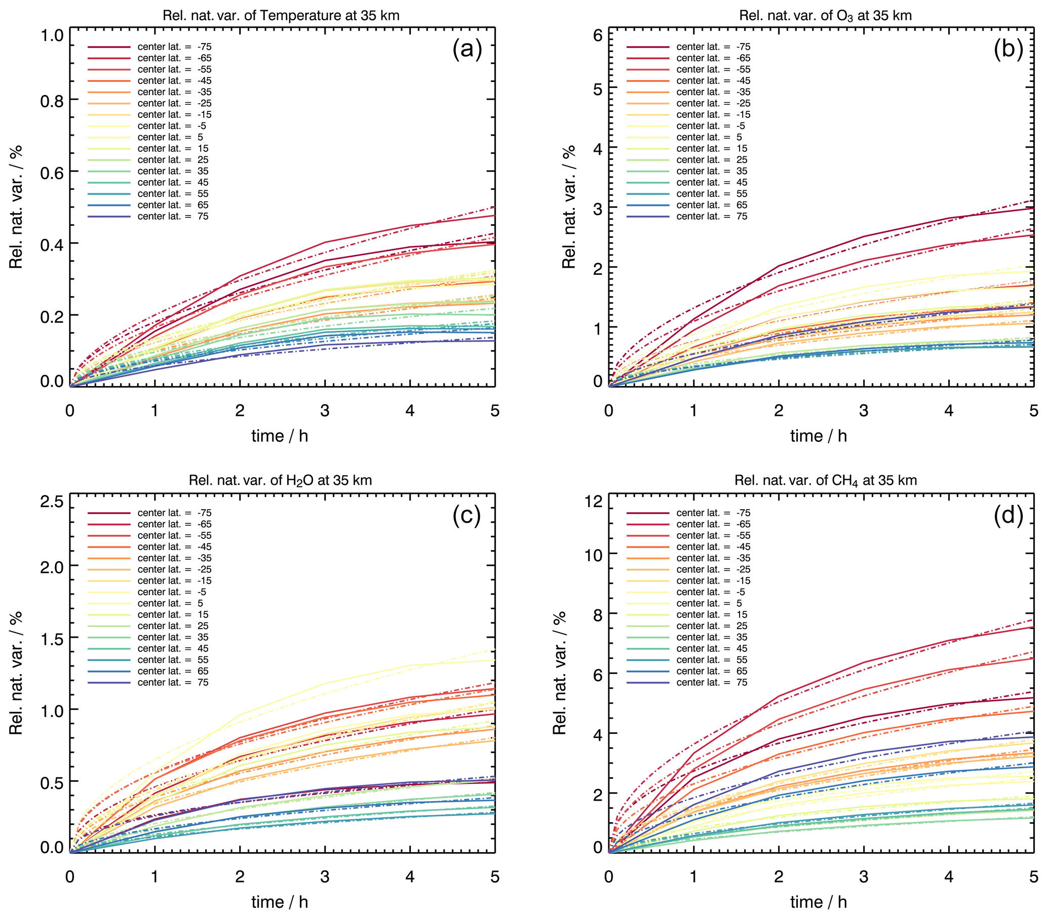
Figure 3 Natural variability as a function of time separation for (a) temperature, (b) O₃, (c) H₂O and (d) CH₄ in the BASCOE model (solid lines) and the proposed parametrization (dashed lines) in different latitude bins.

As pointed out in the Sect. 3.2.1, variability grows very rapidly at high latitudes and distances over 1000 km. Moreover, at low latitudes, the values of variability as a function of the distance mismatch is meaningless at 100 km: it is calculated on the samples from too small to empty, due to the model horizontal resolution. The choice of a 5 h upper limit for the time-dependent variability is driven by the typical values of the time mismatch occurring in satellite validation studies and on the shape of the obtained curves. We calculate the regression coefficients A and γ by minimizing the quantity

$$\begin{array}{}\text{(7)}& \sum _{i=\mathrm{2}}^{\mathrm{10}}{\left(y_i-A{{\mathit{\tau }}_i}^{\mathit{\gamma }}\right)}^{\mathrm{2}}\end{array}$$

via the Sequential Least SQuares Programming (SLSQP) optimizer (Kraft, 1988) and by giving the value at 100 km as a first constraint for A and 0.5 as a first constraint for γ. The obtained regression curves and the initially calculated model curves for some species are shown in Fig. 2 for distance separation and in Fig. 3 for time separation. Note that the assumed parameterization does not apply for a high-latitude case at large distances. The initial and smoothed (regressed) natural variability surfaces as a function of latitude and time separation are shown in Fig. 4 for ozone at 35 km altitude. In a range between 100 and 1000 km, the parametrizations fit the data very well.

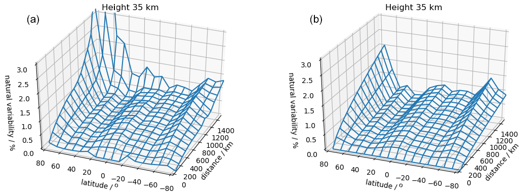
Figure 4 Natural variability of O₃ at 35 km altitude as a function of horizontal distance separation in the BASCOE model for the (a) model fields and (b) regressed fields.

5 Reparametrization on latitudinal gradients

An obvious deficiency of our approach is that the variability fields are calculated from only 1 week of data. Operational constraints did not allow us to generate a better coverage for that many species at the required resolution. The variability, which we have calculated as a function of latitude and distance (time) mismatch, is also dependent on season, as different seasons correspond to different inclinations of the Earth's axis and, intuitively, should all be shifted in latitude as the season changes. There is, however, a way to tackle the problem: if the user is willing to calculate one additional quantity from this data, namely the latitudinal gradients of the gas under validation, then the workaround consists of the reparametrization of the variability of the latitudinal gradients of the species. Latitudinal gradients of a gas are defined as follows:

$$\begin{array}{}\text{(8)}& \left|{\displaystyle \frac{{\text{VMR}}_{l_{\mathrm{1}}}-{\text{VMR}}_{l_{\mathrm{2}}}}{l_{\mathrm{1}}-l_{\mathrm{2}}}}\right|,\end{array}$$

where ${\text{VMR}}_{l_{\mathrm{1}}}$ is the mean VMR of the gas in a latitude band, ${\text{VMR}}_{l_{\mathrm{2}}}$ is the mean VMR in the northward neighboring latitude band, and l₁−l₂ is the width of the latitude band (in our case, this is 10^∘). In the relative version of the latitudinal gradient, this quantity is normalized with respect to the mean VMR in both bands and is multiplied by 100. For a fixed distance (or time) mismatch, as a first approximation, because the variability is calculated as the square root of the variance of differences, and the latitudinal gradients are calculated as differences, we expect a linear dependence of the variability from the latitudinal gradients.

To test the abovementioned theoretical considerations in practice, especially to see if the linear dependence of the natural variability from the latitudinal gradients is the same in different seasons, the link between the natural variability and the latitudinal gradients was tested on the data of a worse resolved model with less species, although using a model for which the data from different seasons were available, namely data from WACCM6.

Figure 5 shows the ozone distributions in each season of WACCM data. The distributions are as expected, and the latitudinal shift in different season is visible; therefore, the data are suitable for our test.

Figure 5 Distribution of O₃ in 1 week of each season in the WACCM model.

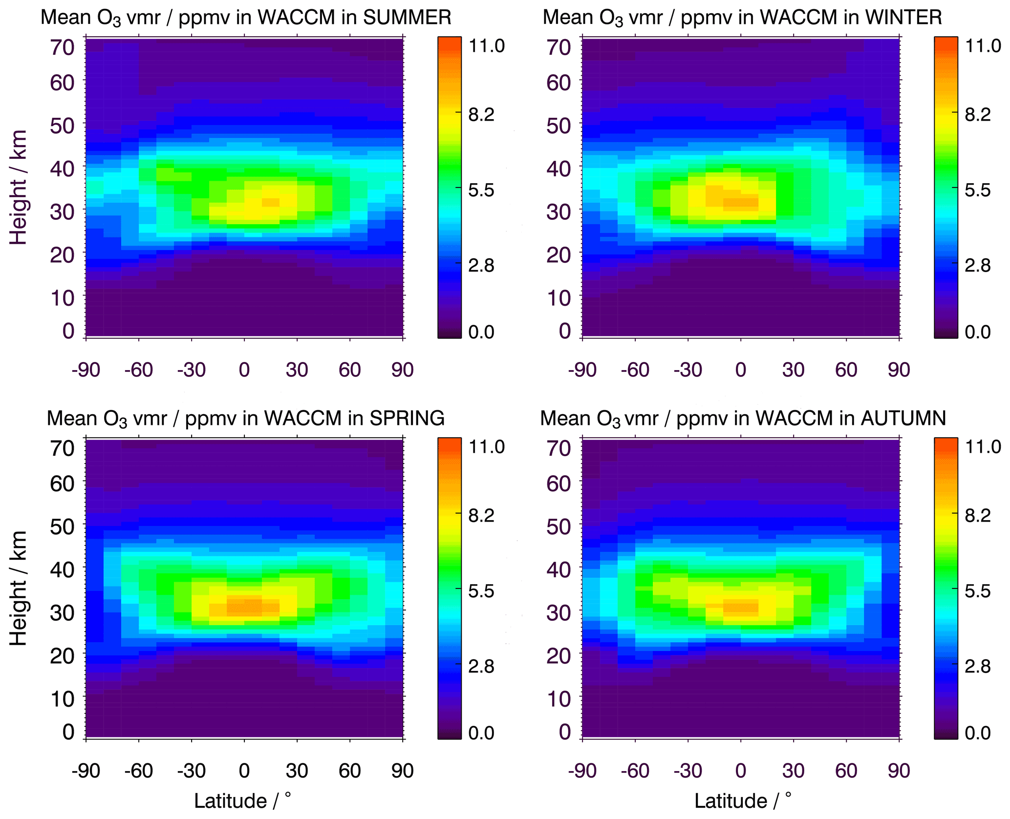
Figures 6, 7 and 8 show the natural variability as a function of latitudinal gradients for a particular distance separation of 400 km in four seasons of WACCM for H₂O at 30 km, O₃ at 35 km and NO at 40 km. Each point in these figures corresponds to one 10^∘ latitude band; for the sake of completeness, we include the points from all of the latitudes. One can observe that the regression lines are similar in all cases, with some deviation in summer and winter that stems from the points corresponding to high (>70^∘) latitudes, which is expected. Similar linear dependencies, which are comparable for different seasons, are observed when changing the 400 km separation distance. This hints at a seasonally independent linear approximation of the natural variability as a function of latitudinal gradients. Hence, the natural variability calculated in just one season and reparameterized on latitudinal gradients of the species provides all of the information needed for the validation exercise in any season. Finally, we would like to remark that the variability fields of well-correlated tracers are close, which provides additional confidence in the method.

Figure 6 Natural variability of H₂O as a function of latitudinal gradients for a 400 km distance separation at 30 km altitude in four seasons in the WACCM model. The horizontal axis corresponds to latitudinal gradients, and the dashed line is the linear regression of plotted points.

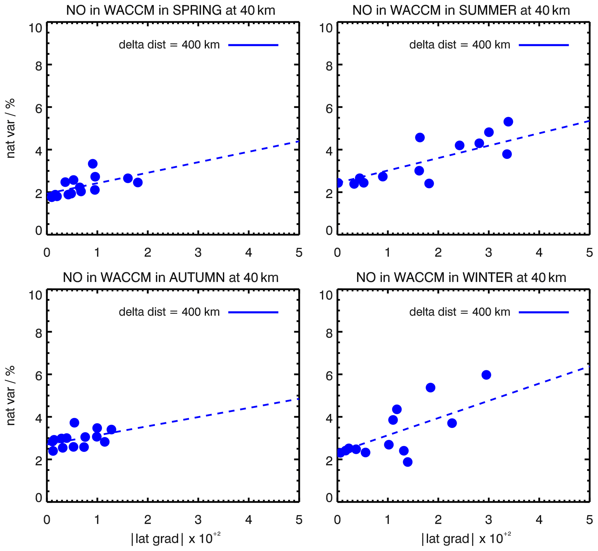
Figure 7 Natural variability of NO as a function of latitudinal gradients for a 400 km distance separation at 40 km altitude in four seasons in the WACCM model.

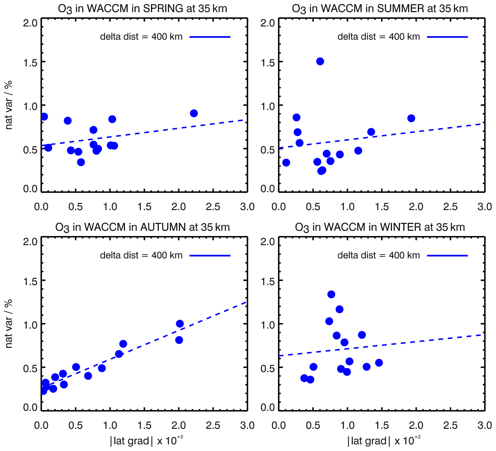
Figure 8 Natural variability of O₃ as a function of latitudinal gradients for a 400 km distance separation at 35 km altitude in four seasons in the WACCM model.

6 What to do in practice: the software

The variabilities as functions of time and distance mismatch are added quadratically, and this provides the final variability value for the chosen co-location criteria. In practice, the users will have to calculate just one additional quantity from the data under validation, namely the latitudinal gradients of the species under validation. This quantity should be calculated on the whole sample in order to increase the significance of the statistics. In addition to the regression coefficient values, we provide a software that uses the species' name (among the 30 available), the distance and time mismatch chosen, the latitude band, the value of the latitudinal gradients of these data and the height as input and then outputs the value of the natural variability of the gas at a given altitude, latitude band and mismatch. If the validation study is performed in a latitude domain larger then 10^∘, the values in the corresponding 10^∘ bands should be added quadratically.

7 Discussion

In the sense of playing devil's advocate, we try to raise possible objections to our method and rebut them. As we do not use model data directly, instead using only differences between model data, the additive model biases cancel out. Critical minds might plead that there could still be multiplicative biases in the model data that would affect our statistics of differences. However, these are not harmful if the gradient-related parametrization is used instead of the latitude–month-related parametrization. The rough reason for this is as follows: a model bias affects the horizontal gradients in the same way as the differences used for our statistics. Thus, the effect of a multiplicative model bias also cancels out.

An obvious objection to our method is that the model data used cover only a short time period and might not be inductively generalizable towards other time periods. We agree that, due to the annual cycle, the typical meteorological regimes are shifted in latitude over the year. However, once again, when the gradient-related parametrization is used, it is likely that the statistics of the correct meteorological regime is chosen, even if it is found at different latitudes to that of the validation experiment. The explanation for this is that the natural variability of mixing ratios of most trace species is predominantly driven by the latitudinal gradients. It goes without saying that this does not hold for fast-reacting species, particularly those that are in photochemical equilibrium.

These parametrizations should not be used where polar vortex dynamics may play a role or for spatial mismatches beyond 1000 km and temporal mismatches beyond 5 h; however, these situations are not the preferred validation scenarios anyway.

8 Conclusions

In validation exercises, a universal excuse used to explain the residual discrepancy between the data is the natural atmospheric variability due to imperfect co-locations. This work is the first attempt to quantify this atmospheric variability for a large sample of atmospheric constituents and to provide the user with a tool to subtract the natural atmospheric variability portion from the residual variability. The fields of natural atmospheric variability as a function of distance and time mismatch were calculated from highly resolved BASCOE model data. The variability data were described with an easy-to-use regression function, and the regression coefficients as well as the software that calculates the value of the corresponding natural variability for given gas, latitudinal gradient, height, and co-location criteria are provided to the community. The independence of the linear approximation of the natural variability as a function of latitudinal gradients from season was demonstrated on WACCM model data. An application of the method to ozone and temperature fields will be provided in upcoming validation papers of version 8 of the MIPAS data.