the Creative Commons Attribution 4.0 License.
the Creative Commons Attribution 4.0 License.
 | 20 Jul 2022
Inter-comparison of atmospheric boundary layer (ABL) height estimates from different profiling sensors and models in the framework of HyMeX-SOP1
Donato Summa
Fabio Madonna
Noemi Franco
Benedetto De Rosa
Paolo Di Girolamo
This paper reports results from an inter-comparison effort involving different sensors and models used to measure the atmospheric boundary layer height (ABLH). The effort took place in the framework of the first Special Observing Period of the Hydrological Cycle in the Mediterranean Experiment (HyMeX-SOP1), with the Raman lidar system BASIL deployed in Candillargues (southern France) and operating in almost continuous mode over the time period September–November 2012. ABLH estimates were obtained based on the application of the Richardson number technique to Raman lidar and radiosonde measurements and to ECMWF-ERA5 reanalysis data. In the effort we considered radiosondes launched in the proximity of the lidar site, as well as radiosondes launched from the closest radiosonde station included in the Integrated Global Radiosonde Archive (IGRA). The inter-comparison effort also includes ABLH measurements from the wind profiler, which rely on the turbulence method, as well as measurements obtained from elastic backscatter lidar signals. The Richardson number approach applied to the on-site radiosonde data is taken as reference. Measurements were carried out throughout the month of October 2012. The inter-comparison is extended to both daytime and night-time data. Results reveal a very good agreement between the different approaches, with values of the correlation coefficient R2 for all compared data pairs in the range 0.94–0.98. Values of the slope of the fitting line in the regression analysis are in the range 0.91–1.08 for daytime comparisons and in the range 0.95–1.03 for night-time comparisons, which testifies to the presence of the very small biases affecting all five ABLH estimates with respect to the reference ABLH estimate, with slightly smaller bias values found at night. Results also confirm that the combined application of different methods to the sensors and model data allows us to get accurate and cross-validated estimates of the ABL height in a variety of weather conditions. Correlations between the ABLH measurements and other atmospheric dynamic and thermodynamic variables, such as CAPE (convective available potential energy), friction velocity and relative humidity, are also evaluated to infer possible mutual dependences.
- Article
(6762 KB) - Full-text XML
- BibTeX
- EndNote


The atmospheric boundary layer (ABL) is the lowest portion of the atmosphere, directly in contact with and influenced by the Earth's surface, which reacts to the combined action of mechanical and thermal forcing factors. In this layer, turbulent air motion and vertical mixing induced by shear and buoyancy forces (Stull, 1988) cause rapid fluctuations of a variety of physical quantities such as flow velocity, temperature and moisture. The variability in these quantities is often exploited to estimate the atmospheric boundary layer height (ABLH).
The evolution of the ABL structure and height has an important impact on meteorology. Accurate measurements of the ABLH allow air quality and weather forecast models to be validated and several physical schemes to be improved like, among others, the boundary layer turbulence and shallow convection parameterizations. However, in many cases, the complexity of the phenomena occurring within the ABL and the influence of advection and local accumulation processes prevents an unambiguous determination of the ABLH from, for example, elastic lidar signals, especially when aerosol stratifications are present within the ABL (Haeffelin et al., 2012). Various methods have been reported in the literature to estimate the ABLH from the vertical profiles of different atmospheric variables. The five most used approaches are (1) the turbulence method (Stull, 1988), (2) the temperature gradient method (Bianco and Wilczak, 2002; Seidel at al., 2012), (3) the Richardson number method (Joffre et al., 2001; Sicard et al., 2006), (4) the wind (Melgarejo and Deardorff,1974) and wind shear (Hyun et al., 2005) profile methods, and (5) the combined cloud top and relative humidity method (Lenschow et al., 2000), this latter being applicable only in the presence of stratocumulus-topped boundary layers. A review of these different methodologies was reported by H. Dai et al. (2014). In the present research effort we compare ABLH measurements obtained through the application of the Richardson number technique to a variety of sensors and model data, namely the Raman lidar BASIL, radiosondes and ECMWF-ERA5 analysis data. These results are also compared with ABLH measurements from a wind profiler and from elastic backscatter lidar signals.
The Richardson number method relies on the identification of Richardson number gradients which are an important diagnostic indicator of dynamic flow stability. This method assumes the ABLH to be the level where the so-called “bulk Richardson number” exceeds a specific threshold value, Ribc. The vertical profile of Rib can be calculated from wind speed and potential virtual temperature profiles, as originally reported in Hanna (1969) and extensively described in, for example, Stull (1988) and Garratt (1994). As the estimate of the Richardson number requires information on both wind and thermodynamic profiles, the application of this approach to Raman lidar data relies on thermodynamic profile measurements from this sensor and wind measurements from simultaneous and co-located radiosondes as the wind measurements are not available from the Raman lidar.
ABLH measurements carried out by the wind profiler rely on the turbulence method, which identifies the ABLH as the depth of the lowest continuous turbulence layer (Stull, 1988). The turbulent region is determined by tracking the fluctuations of the different wind components (U,V, and W), for example through a high-pass wavelet filter (Wang et al., 1999). Such fluctuations can be identified in wind lidar and wind profiler data, but measurements can also be performed with radiosondes and tethered balloons or in situ sensors on board scientific aircraft.
An alternative and effective method to determine the ABLH relies on the strong sensitivity of elastic backscatter lidar signals to suspended aerosol particles and their gradient and on the circumstance that aerosols, being more abundant within the ABL than in the free troposphere, can act as tracers of atmospheric motions. Such an approach, extensively used in the present inter-comparison effort, both in daytime and night-time, is described in detail in the following section.
Another convenient, reliable and widely used approach to determine the ABL height and structure both in daytime and night-time is based on the identification of local maxima in potential temperature vertical gradient profiles as measured by meteorological radiosondes (Cramer, 1972; Oke, 1988; Stull, 1988; Sorbjan, 1989; Garratt, 1992; Van Pul et al., 1994; De Wekker et al., 1997; Martucci et al.,2007; Behrendt et al., 2011).
This paper does not represent the first research effort dedicated to an extensive inter-comparison of different ABLH sensors and methodologies. In a previous paper, Seibert et al. (2000) compared different methods to estimate the ABLH from radiosondes and other instruments and carefully examined advantages and shortcomings of the investigated approaches. In the present paper ABLH estimates obtained through the application of the Richardson number technique to two sensors (a Raman lidar and radiosondes) and to the ECMWF-ERA5 model reanalysis data are compared with ABLH measurements from the wind profiler and from elastic backscatter lidar signals. The capability of the Raman lidar BASIL to perform high-resolution and accurate profile measurements of atmospheric temperature and water vapour, as well as particle backscatter profile measurements, allows us to obtain ABLH estimates based on both the application of the Richardson number approach and the use of elastic backscatter lidar signals.
However, accurate estimates of the ABL height and structure in complex terrains or under complex meteorological conditions remain problematic. A variety of authors have tried to address this challenging issue. Among others, Herrera-Mejía and Hoyos (2019) studied the spatio-temporal evolution of the ABL in a narrow, highly complex terrain located in the Colombian Andes, where convective activity, as a result of aerosol dispersion, increases the uncertainty affecting the estimate of ABLH. Staudt (2006) provided a comprehensive analysis of the ABLH variability over complex terrains in the Bavarian Alpine foreland, based on the use of multi-sensor data collected during the field experiment SALSA 2005. Che and Zhao (2021) assessed the effectiveness of different approaches to characterize the summer ABLH variability over the Tibetan Plateau, this region being characterized by elevations exceeding 4000 m and complex land surface processes and boundary layer structures.
Coming to the characterization of the ABLH in cloudy conditions, Dang et al. (2019a, b) investigated different approaches, with a specific focus on reducing the interference of the residual and cloud layers on ABLH determination. Manninen et al. (2019) demonstrated the capability of Doppler lidars to determine the ABLH in both clear-sky and cloud-topped conditions, with some limitations during precipitation events. Furthermore, Liu et al. (2022) proposed an approach to estimate ABLH from elastic backscatter lidar data under complex atmospheric conditions based on the use of machine learning methods.
However, both the results from these previous papers and the conclusions reached in the present paper clearly indicate that a proper characterization of the ABL height and structure in all weather conditions requires the combined application of different approaches and datasets. This approach allows us to overcome the possible dependence of each single sensor/method on a specific meteorological parameter, thus drastically reducing potential biases affecting ABLH estimates (C. Dai et al., 2014). Additionally, multi-sensor approaches have been demonstrated to be more robust and perform better under variable stable and unstable weather conditions (Joffre et al., 2001).
The paper outline is the following. Section 2 illustrates the different methods considered in the research effort to determine the ABLH. Section 3 describes the profiling sensors and model data involved in the inter-comparison effort. Section 4 illustrates the results from the inter-comparison effort. Finally, Sect. 5 provides a summary, concluding remarks and indications for possible future follow-on studies.
2.1 Richardson number method
This method assumes the ABLH to be the level where the so-called “bulk Richardson number” exceeds a specific threshold value, Ribc. Rib at height z can be calculated from the wind speed and the potential virtual temperature values at z and at surface level, as originally reported in Hanna (1969) and extensively described in, for example, Stull (1988) and Garratt (1994). In the present research effort the bulk Richardson number has been computed through the following expression:
where θv(0) and θv(z) are the virtual potential temperatures at surface and at height z, respectively, is the buoyancy parameter, and u(z) and v(z) are the horizontal wind-speed components at height z, respectively.
Threshold values of the Richardson number Ribc have been reported in a variety of literature papers (among others, Zilitinkevich and Baklanov, 2002; Jericevic and Grisogono, 2006; Esau and Zilitinkevich, 2010). Reported values are in the range 0.15–1.0, with the most used values in the range 0.25–0.5. One important cause of the large variability in Rib is the thermal stratification of the ABL. For example, Vogelezang and Holtslag (1996) reported Ribc values of 0.16–0.22 for a nocturnal, strongly stable ABL and of 0.23–0.32 for a weakly stable ABL. For unstable ABLs, a Ribc value larger than 0.25 is usually needed (Zhang et al., 2014).
The ABLH is found by assessing the altitude level where Rib(z) reaches the Ribc. In the present research effort we are considering Ribc=0.25 in stable boundary layers and Ribc=0.45 in unstable boundary layers.
In the present research effort we generally considered the layers to be stable during the evening, night and early morning periods, while layers were assumed to be unstable during the late mornings and afternoons in clear-air conditions. The period September–November 2012 was selected for the field campaign because of the specific focus on convection of the Hydrological Cycle in the Mediterranean Experiment (HyMeX) first Special Observing Period (SOP1). Within this 3-month period, intense observation periods (IOPs) were typically selected when convective instability conditions were present. Thus, the number of cases characterized by unstable layers is predominant. Conditions are found to be persistently unstable during the IOP on 18–19 October and in the period 16–22 October. The presence of stable or unstable conditions was verified based on the use of the “lifted index”, obtained from ERA5 model analysis data (see Fig. 5).
The main uncertainty affecting the ABLH estimate based on the application of the Richardson number is related to its sensitivity to atmospheric stability conditions and to the sounding vertical resolution (Seidel et al., 2012). The ABLH is obtained from both the radiosonde and model data using the above-described algorithm, which is applied from the surface upwards. In the case the ABLH falls in between two levels, a linear interpolation is applied to determine its exact position.
In the determination of the bulk Richardson number through Eq. (1) the virtual potential temperature and horizontal wind-speed component profiles are needed. The vertical profile of the potential virtual temperature can be expressed as follows:
where P0 is the standard pressure (1 atm), T(z) is the temperature profile, P(z) is the pressure profile, and is the water vapour mixing ratio profile.
Vertical profiles of T(z) and are available from all sensors and models involved in the inter-comparison effort, namely the Raman lidar, the radiosondes launched on-site and those from the closest Integrated Global Radiosonde Archive (IGRA) radiosonde station and the ECMWF-ERA5 analysis data, with the only exception being the wind profiler. For most sensors, vertical profiles of P(z) are obtained by vertically extrapolating the surface pressure value P0. The vertical profiles of the horizontal wind-speed components u(z) and v(z), which are needed to quantify the bulk Richardson number, are also available from the same sensors and models, with the only exception being the Raman lidar, which only provides the humidity and temperature profile measurements needed to determine the virtual potential temperature profile. In this case, the computation of the Richardson number is completed with the inclusion of wind-speed profile measurements from the simultaneous and co-located radiosondes launched in Candillargues.
2.2 Determination of the ABLH from elastic backscatter lidar measurements
Lidar systems are presently able to provide continuous measurements of atmospheric variables, such as particle backscatter, temperature or water vapour concentration profiles, and thus can provide continuous measurements of the ABLH. In the present research effort we consider Raman lidar measurements from BASIL collected in southern France in the period September–November 2012 in the frame of HyMeX-SOP1. We focus our attention on the measurements carried out during October 2012.
There are several methodologies to determine the ABLH from elastic lidar signals which rely on the circumstance that aerosols are more abundant within the ABL than in the free troposphere and that they can act as tracers of atmospheric motions. A widely used methodology relies on the detection of vertical gradients in elastic backscatter lidar signals associated with aerosol concentration gradients.
The elastic lidar equation, expressed in terms of number of collected photons as a function of height, is defined as follows:
where λ0 is the emitted and received lidar wavelength, z is the vertical height, is the number of laser-emitted photons, O(z) is the overlap function, A is the telescope collection area, βmol(z) and βpar(z) are the backscatter coefficients for molecules and particles, respectively, Tmol(z) and Tpar(z) represent the molecular and particle contribution to atmospheric transmissivity, respectively, and Pbgd is the background signal associated with solar irradiance and detectors' noise. In order to compress the signal dynamical variability and define an uncalibrated quantity proportional to total (molecular + particle) attenuated backscattering coefficient, it is often preferable to make use of the range-corrected signal (RCS), which is defined as follows:
As the larger vertical variability in the RCS is associated with aerosol vertical gradients, the ABLH is estimated from the height derivative of RCS through the following expression:
Transitions between different aerosol layers are identified with the minima in Eq. (5), with the highest amplitude minimum, i.e. the largest aerosol gradient, typically indicating the ABLH. This approach relies on the strong sensitivity of elastic backscatter lidars to suspended aerosol particles and their gradient and on the capability of aerosols to act as tracers of atmospheric motions. It is to be specified that ABLH estimates determined through this approach identify the convective boundary layer height during the day, when convective activity is on, and the residual layer during the early morning, the late afternoon and the night, when convective activity is strongly reduced or suppressed.
For the specific purposes of our present study, the elastic backscatter signal at 355 nm, P355(z), is considered in Eq. (3) (Summa at al., 2013; Vivone et al., 2021). Overlap effects affect lidar signals in the lower few hundred metres but have marginal effects on gradient measurements and consequently on the accuracy of ABLH estimates. In fact, overlap effects may determine a compression of the elastic signal dynamics, and consequently a reduction in the amplitude of the detected range-corrected signal gradients, but will not cancel these gradients, making the detection of the ABLH still effective. Overlap effects are more pronounced when determining the night-time ABLH, especially when this height is within a few tens of metres and may fall in the lidar-blind region.
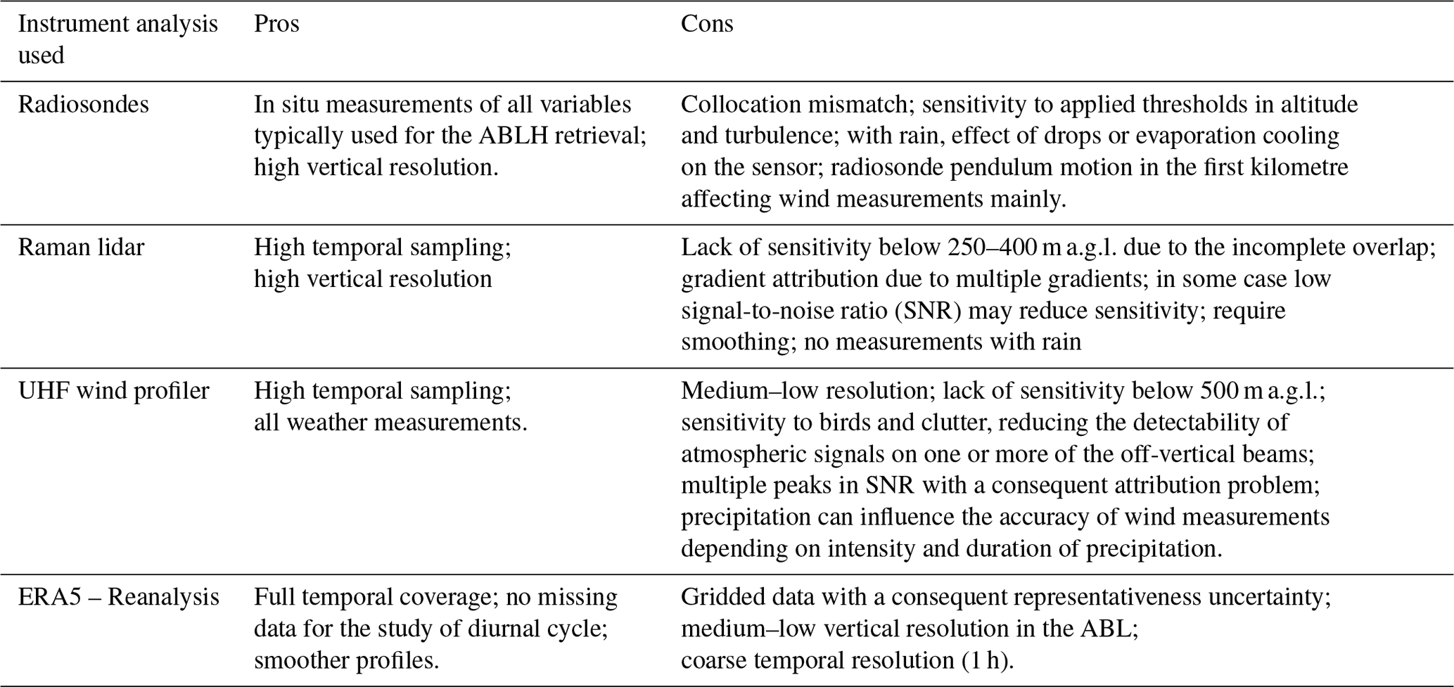
This section illustrates the characteristics, specifications and performance of the ground-based instruments and models used in the present research effort to estimate the ABLH: a Raman lidar system, a UHF wind profiler, co-located radiosoundings and those from the nearest site available in the IGRA, and the ECMWF-ERA5 reanalysis. Instrumental pros and cons and potential sources of bias of the different instruments and reanalysis data are reported in Table 1.
Table 1Pros and cons of the considered instruments/reanalysis and their potential sources of bias.
3.1 BASIL system
The University of Basilicata ground-based Raman lidar system (BASIL) was deployed in the Cévennes-Vivarais (CV) site (Candillargues, southern France; 43∘37′ N, 4∘4′ E; elevation: 1 m; Fig. 1) and operated between 5 September and 5 November 2012, collecting more than 600 h of measurements, distributed over 51 measurement days and 19 intensive observation periods (IOPs; Di Girolamo et al., 2016; Stelitano et al., 2019). BASIL is capable of performing high-resolution and accurate measurements of atmospheric temperature and water vapour, both in daytime and night-time, based on the application of the rotational and vibrational Raman lidar techniques, respectively, in the UV (Di Girolamo et al., 2004, 2009a, 2017; Bhawar et al., 2011). This measurement capability makes BASIL an effective tool for the characterization of water vapour inflows in southern France, which are a key ingredient of the heavy precipitation events taking place in the north-western Mediterranean Basin. BASIL also performs profile measurements of particle backscatter at 355, 532, and 1064 nm, particle extinction at 355 and 532 nm, and particle depolarization at 355 and 532 nm (Di Girolamo et al., 2009b, 2012a, b, 2017).
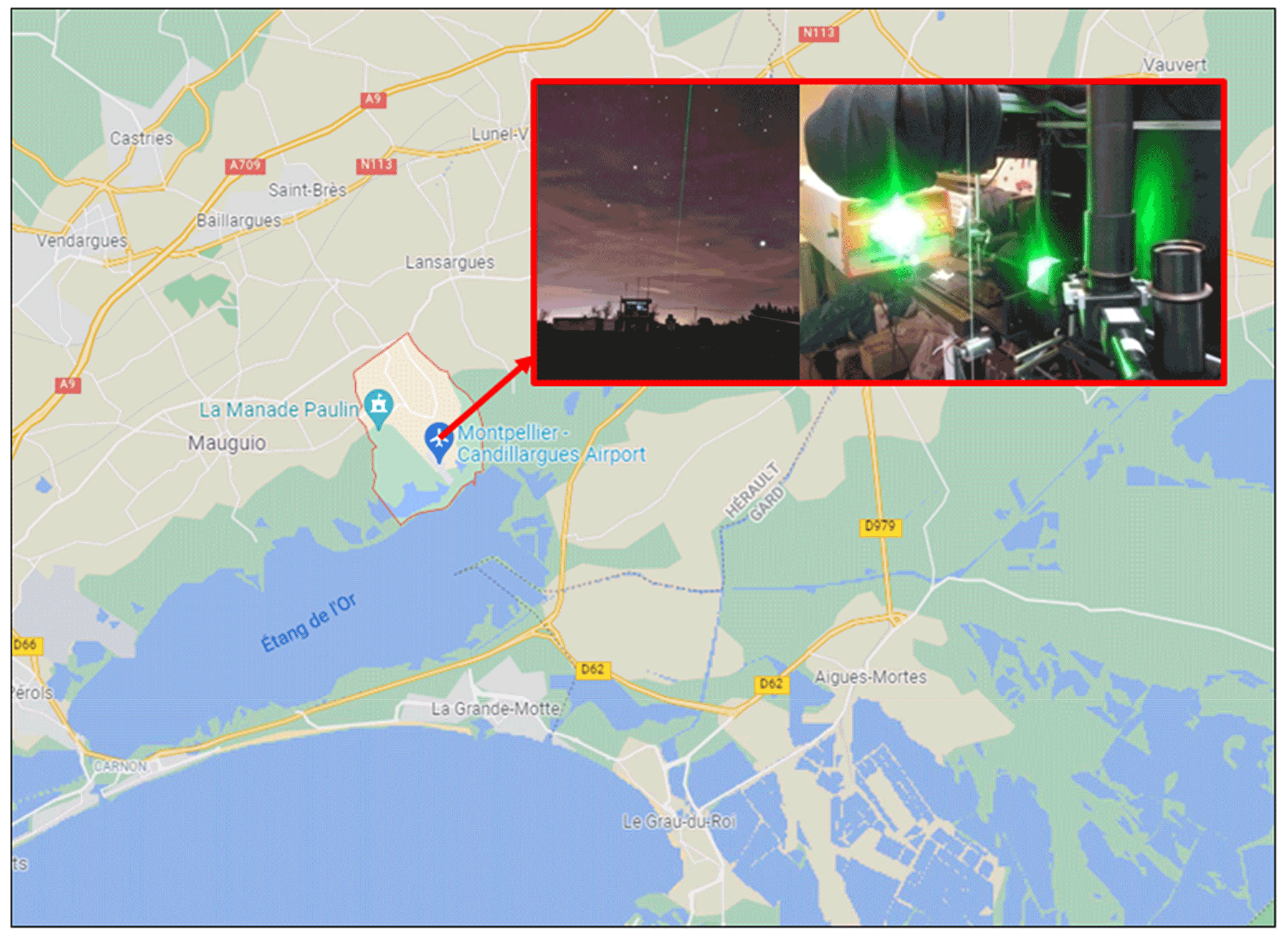
Figure 1Location and two images of the Raman lidar system BASIL operated during HyMeX-SOP1 (© Google Maps 2021).
BASIL makes use of a Nd:YAG laser source capable of emitting pulses at 355, 532 and 1064 nm, with single pulse energies at 355 nm, i.e. the wavelength used to stimulate rotational and rotational–vibrational Raman scattering from atmospheric molecules, of 500 mJ (average optical power of 10 W at a laser repetition rate of 20 Hz). The receiver includes a Newtonian telescope (45 cm diameter primary mirror). Data are sampled with a rough vertical and temporal resolution of 7.5 m and 10 s, respectively, but vertical and temporal smoothing is typically applied when processing water vapour, temperature and particle backscatter measurements for the purpose of estimating the ABLH. In the present study we considered a vertical and temporal resolution of 30 m and 5 min, respectively. Based on these vertical and temporal resolutions, water vapour and temperature profile measurements from BASIL extend from the proximity of the surface (50–100 m above station level) up to km (day/night) and km (day/night), respectively.
3.2 UHF wind profiler
Wind profilers are quite effective and very often used in long-term ABLH measurements as a result of their unattended operation over extended observation periods and the availability of networks of operational wind profilers over wide areas of the globe. However, the operational use of wind profilers is limited by their lack of sensitivity within the surface atmospheric layer (up to 500 m), which prevents an adequate monitoring of the ABLH and structure at night or in the presence of shallow ABLs.
The five-beam wind profiler (WPR) used in this study was also deployed in Candillargues, approximately 100 m away from the Raman lidar. The system is manufactured by Degreane (model PCL 1300) and operates in the UHF band with a primary frequency at 1.274 GHz. A detailed description of the WPR, its specifications, main working parameters, data processing methodologies and delivered geophysical products is given in Saïd et al. (2016). The WPR operated almost continuously throughout the duration of HyMeX-SOP1 (Saïd et al., 2018). For the purpose of the ABLH measurements reported in this paper, the WPR was operated in low mode, with a pulse length of 1 µs, which allows the lower troposphere to be sampled from 0.15 to 5.7 km a.g.l., with a vertical resolution of 150 m. The methodology applied to determine the ABLH relies on the identification of a distinctive strong peak in the WPR time–height reflectivity plot (Gage et al., 1990), which is associated with turbulence-generated radio refractive index fluctuations and associated atmospheric thermodynamic parameter fluctuations, though the strength of this peak may depend also on other factors. Wind profiling radars are sensitive to turbulence scales equal to half the radar wavelength. At 1.274 GHz, this wavelength is ∼20 cm. Therefore the wind profiler is sensitive to turbulent eddies, with spatial dimensions of ∼10 cm causing fluctuations in the radio refractive index. In the boundary layer, essentially all scales of turbulence exist from 1 cm wavelengths up. Wind velocity measurements rely on the detection of the Doppler shift, assuming that fluctuations in the radio refractive index, dependent on atmospheric thermodynamic parameters, are carried along the mean wind flow.
3.3 Radiosoundings
A radiosonde launching facility was installed and set up in Candillargues in the proximity of the Raman lidar shortly before the start of HyMeX-SOP 1 in early September 2012. Radiosondes, manufactured by Vaisala (model: RS92-SGP), were launched without a predefined schedule, primarily during the intensive observation periods, with a launching rate of up to one launch every 1.5 h. The radiosondes were set to provide vertical profiles of atmospheric pressure, temperature, humidity, and wind direction and speed during both the ascent and descent phases. For the accuracy of pressure, temperature, humidity and wind sensors on board Vaisala RS92 radiosondes (https://www.vaisala.com/sites/default/files/documents/RS92SGP-Datasheet-B210358EN-F-LOW.pdf, last access: 18 June 2022).
3.4 IGRA database
ABLH estimates were also inferred from the radiosondes launched from the nearest Integrated Global Radiosonde Archive (IGRA) radiosounding station. The specific IGRA station considered in our study is Nîmes-Courbessac (43.8569∘ N, 4.4064∘ E; 60 m a.s.l., World Meteorological Organization – WMO – index =7645), typically carrying out four radiosonde launches per day. The IGRA radiosondes are characterized by a lower resolution than the Vaisala RS92 radiosondes. Consequently, data from the two radiosondes have been interpolated on a common height array, with the deviations associated with the interpolation procedure having been verified to be negligible. The launched GPS radiosondes are manufactured by Meteomodem (model: M10). IGRA is the most comprehensive, authoritative collection of historical and near-real-time radiosonde and pilot balloon observations, with global coverage maintained and distributed by the National Oceanic and Atmospheric Administration's National Centers for Environmental Information (NCEI). Data were extracted from the IGRA DataBase (IGRA-DB; version V2), which was released in 2016 (Durré et al., 2018) and includes enhanced-quality data with respect to the previous database version (version V1). The performance of M10 radiosondes has been assessed and verified during the WMO 2010 radiosonde inter-comparison effort in Yangjiang (Nash et al., 2010; Madonna et al., 2020, 2021).
3.5 ECMWF-ERA5
ECMWF-ERA5 is the latest reanalysis produced by ECMWF, which includes hourly data on regular latitude–longitude grids, with a resolution (Hersbach et al., 2020). Atmospheric parameters are provided at 2 m and at 36 additional pressure levels. ERA5 is publicly available through the Copernicus Climate Data Store (CDS, https://cds.climate.copernicus.eu/, last access: 25 May 2021).
In order to properly carry out the comparisons, the nearest ERA5 grid point to the Raman lidar site was considered. We assume the representativeness uncertainty associated with the use of the nearest grid point to be comparable with the uncertainty affecting most interpolation approaches (e.g. kriging, bilinear interpolation). In general, reanalysis reliability can considerably vary depending on the location, time and selected atmospheric variable (Dee et al., 2016).
4.1 Climatological variability throughout October 2012
In this section we illustrate and discuss the results obtained in the comparison of ABLH estimates obtained from different sensors' measurements (Raman lidar BASIL and radiosondes) and model data (ECMWF-ERA5 analysis) through the application of the Richardson number technique. The inter-comparison effort also includes ABLH measurements from the wind profiler, which rely on the turbulence method, as well as measurements obtained from elastic backscatter lidar signals.
We first provide a more climatological assessment, focusing on the evolution of the ABLH throughout the month of October 2012. A separate comparison has been carried out for daytime and night-time cases, at 12:00 and 00:00 UTC, respectively (local time is UTC+02:00 in this period of the year). The considered sensors and models are averaged over a half-hour time interval centred over the comparison time, i.e. over the interval 11:45–12:15 UTC in daytime and 23:45–00:15 UTC at night. Figure 2 illustrates the time evolution of the ABLH as measured/modelled through the above-mentioned sensors, models and approaches, with Fig. 2a1 focusing on daytime cases and Fig. 2a2 on night-time cases. The figure includes six distinct ABLH estimates: ABLHs obtained through the application of the Richardson number method to (i) the Raman lidar data, the radiosonde data (considering separately (ii) radiosondes launched on-site and (iii) radiosondes launched from the closest IGRA station), (iv) the ECMWF-ERA5 analysis data, and (v) ABLHs obtained from wind profiler and (vi) ABLHs obtained from elastic backscatter lidar signals. Results reveal a generally good agreement between the six different estimates both in daytime and night-time, all of them revealing the major features associated with ABLH monthly variability. However, percentage differences may be large especially during the night when the ABL becomes shallow. During the month of October 2012, approximately 60 % of the night-time ABLH values are found to not exceed 300 m. Percentage differences in excess of 100 % are found only 2 times in this period and characterize the comparison of BASIL vs. the on-site radiosondes, with the former of these two sensors having a limited sensitivity below 250 m as a result of the presence of overlap effects and a blind vertical region.
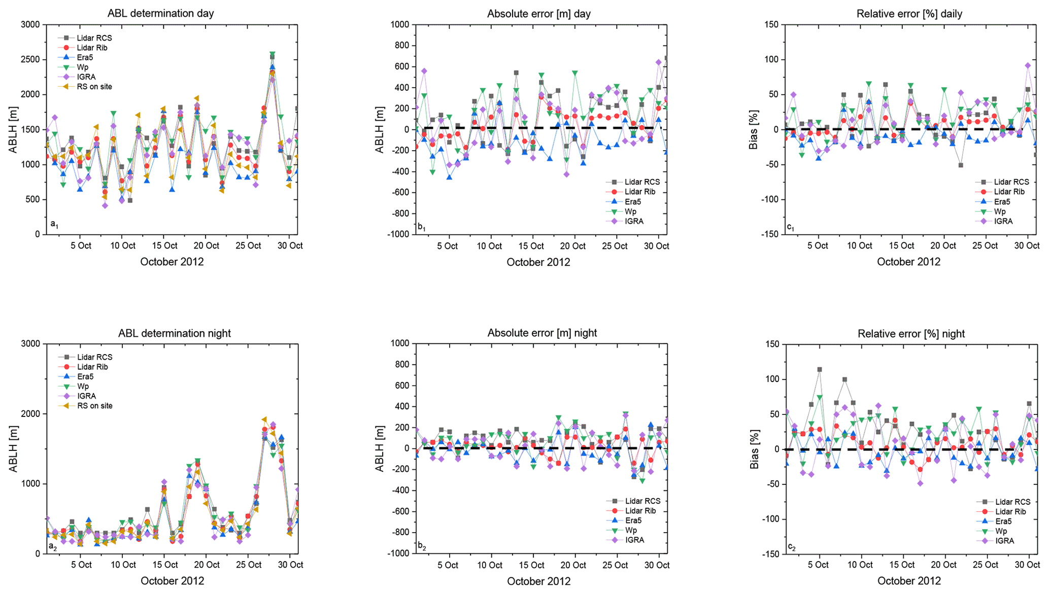
Figure 2Time evolution over the time period 1–31 October 2012 of the six distinct ABLH estimates illustrated in the paper. Panel (a1) illustrates the daytime comparison, while panel (a2) illustrates the night-time comparison. “Lidar Rib” stands for ABLH estimates obtained through the Richardson number method applied to the Raman lidar data, “RS on-site” stands for ABLH estimates obtained through the Richardson number method applied to the on-site radiosonde data, “IGRA” stands for ABLH estimates obtained through the Richardson number method applied to the IGRA radiosonde data, “ERA5” stands for ABLH estimates obtained through the Richardson number method applied to the ECMWF-ERA5 analysis data, “WP” stands for ABLH estimates obtained from wind profiler, and “Lidar RCS” stands for ABLH estimates obtained from range-corrected elastic backscatter lidar signals. Panels (b1)–(b2) and (c1)–(c2) represent the daytime deviations, expressed both in metres and in percentage (%), between the ABLH estimate obtained through the application of the Richardson number approach to the on-site radiosonde profiles and the five remaining ABLH estimates. Panels (b1) and (c1) illustrate the daytime comparison, while panels (b2) and (c2) illustrate the night-time comparison.
The Richardson number approach applied to the on-site radiosonde profiles is the most reliable approach (lowest bias), and, assuming this approach as bias-free, it can be considered as reference. Figure 2b1 and c1 illustrate the daytime deviations, expressed both in metres and in percentage (%), respectively, between the five remaining ABLH estimates and the reference approach, while Fig. 2b2 and c2 illustrate the night-time deviations. These values are also reported in Table 2. Most deviation values are within ±200 m and ±20 %. Again, larger deviation values are found to characterize those comparisons considering lidar-based night-time estimates of the ABLH as a result of the above-mentioned overlap effects and the presence of a blind vertical region.
Table 2Biases, expressed both in metres and in percentage (%), of the different ABLH estimates with respect to the one obtained through the application of the Richardson number approach to the on-site radiosonde profiles. The data cover the month of October 2012 and are separately listed for daytime (12:00 UTC) and night-time (00:00 UTC) comparisons.
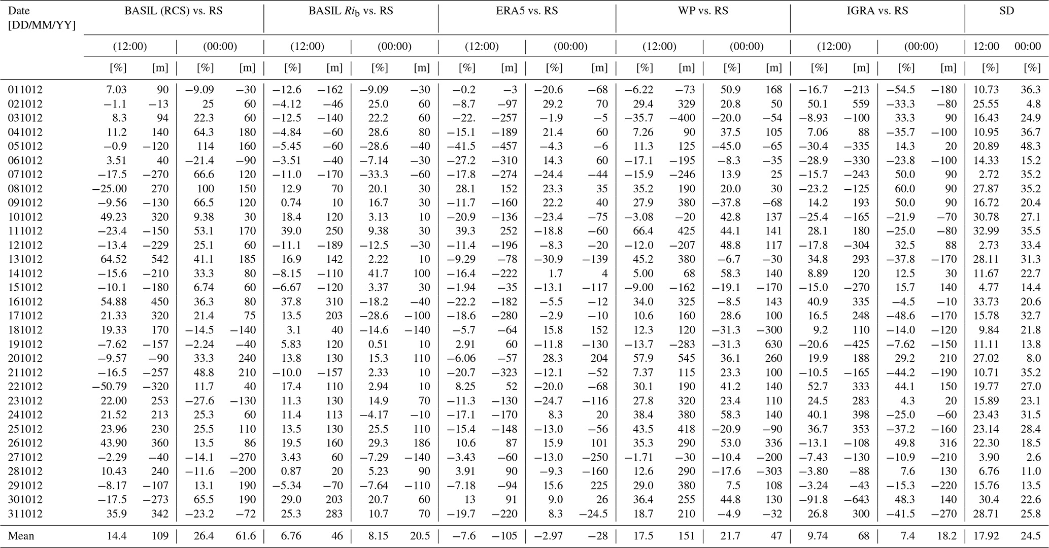
The mean bias throughout the month of October 2012 of each ABLH estimate with respect to the reference value has also been computed. The smallest deviations are observed for night-time comparisons, with absolute mean biases in the range 18.2–61.6 m and relative mean biases in the range 3.0 %–26.4 %. More specifically, smallest biases are found to characterize the ABLH estimates obtained through the application of the Richardson number method (18.2 m and 7.4 % for the IGRA radiosondes, 20.5 m and 8.15 % for the Raman lidar BASIL, and −28 m and −2.97 % for ECMWF-ERA5 analysis), while slightly large bias values are found to characterize ABLH estimates from the wind profiler (47 m and 21.7 %) and ABLH estimates from elastic backscatter lidar signals (61.6 m and 26.4 %). The slightly smaller ABLH values characterizing ECMWF-ERA5 analyses are probably to be attributed to the systematically smaller values of the water vapour mixing ratio and the wind v component from ECMWF-ERA5 with respect to those from other sensors.
Slightly larger absolute deviations are observed for daytime comparisons, with absolute biases in the range 46–151 m and percentage biases in the range 6.8 %–17.5 %. Again, smaller biases are found to characterize night-time ABLH estimates obtained through the application of the Richardson number method (46 m and 6.76 % for the Raman lidar BASIL, 68 m and 9.74 % for the IGRA radiosondes, and 105 m and 7.6 % for ECMWF-ERA5 analysis), while larger values are found to characterize ABLH estimates from the wind profiler (151 m and 17.5 %) and ABLH estimates from elastic backscatter lidar signals (109 m and 14.4 %). In general, there is a negative bias in ERA5. This is because for the parameters q and v, which are necessary for the computation of Rib when comparing on-site radiosondes with ERA5, we often found a negative bias of up to 50 % for water vapour mixing ratio and up to 20 % for wind speed, while temperatures are quite irrelevant.
Figure 3 compares the different ABLH estimates in terms of scatter plots. Each scatter plot includes 31 data points, one per day, throughout the month of October 2012. Again, the different ABLH estimates are compared both in daytime (panels a1–e1 in Fig. 3) and at night (panels a2–e2). A linear fit is applied to the data points using a linear regression function passing through zero, with the form . X are the ABLH reference values, and Y are the values from the five remaining ABLH estimates. The term A represents the slope of the fitting line and provides an alternative estimate of the bias of each of the five ABLH estimates with respect to the reference, while the correlation coefficient R2 of the linear fit quantifies the degree of agreement between the compared ABLH estimates. Values of slope and R2 for each ABLH estimate are reported in Table 3a for daytime comparisons and in Table 3b for night-time comparisons. All values of R2 are in the range 0.94–0.98, which testifies to the high level of agreement between the different ABLH estimates both in daytime and at night, while all values of slope are in the range 0.91–1.08 for daytime comparisons and in the range 0.95–1.03 for night-time comparisons, which testifies the very small bias affecting all five ABLH estimates with respect to the reference estimate. Again, slightly larger biases are observed for daytime comparisons than for night-time, this confirming the results already illustrated in the preceding part of the paper.
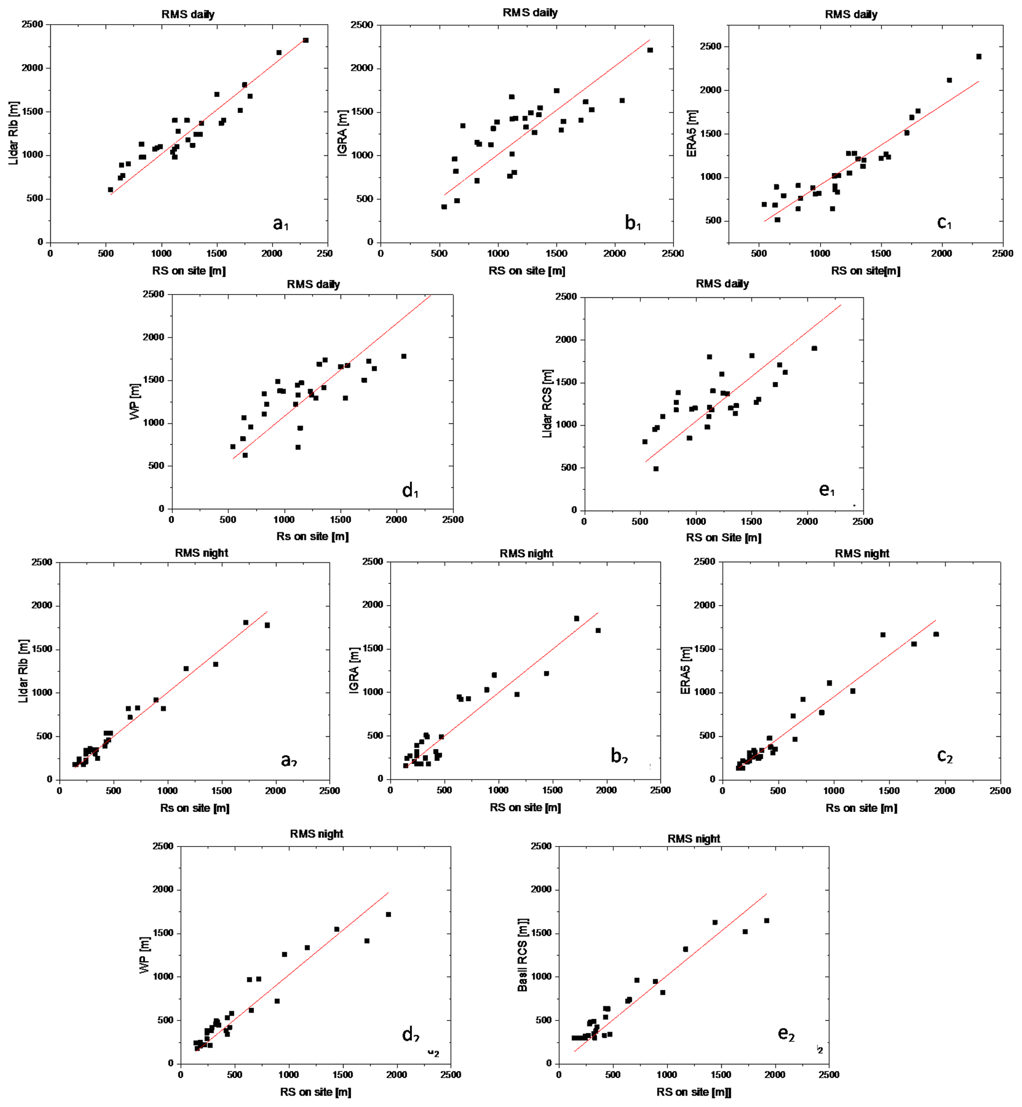
Figure 3Comparison of the different ABLH estimates expressed in terms of scatter plots. On the x axes of each plot are the ABLH reference values obtained through the application of the Richardson number approach to the on-site radiosonde profiles, while on the y axes are the values from the five remaining ABLH estimates. Panels (a)–(e) represent daytime comparisons and panels (f)–(j) night-time comparisons. Panels (a1) and (a2): “Lidar Rib” vs. “RS on-site”; panels (b1) and (b2): “IGRA” vs. “RS on-site”; panels (c1) and (c2): “ERA5” vs. “RS on-site”; panels (d1) and (d2) “WP” vs. “RS on-site”; panels (e1) and (e2): “Lidar RCS” vs. “RS on-site”. The red lines represent the linear fit applied to the data points using a linear regression function with the form .
Table 3Results from the regression analysis, with values of the correlation coefficient R2 and the regression line slope A, with its standard deviation σ(A). Results are reported for both daytime (panel a, 12:00 UTC) and night-time (panel b, 00:00 UTC) comparisons.
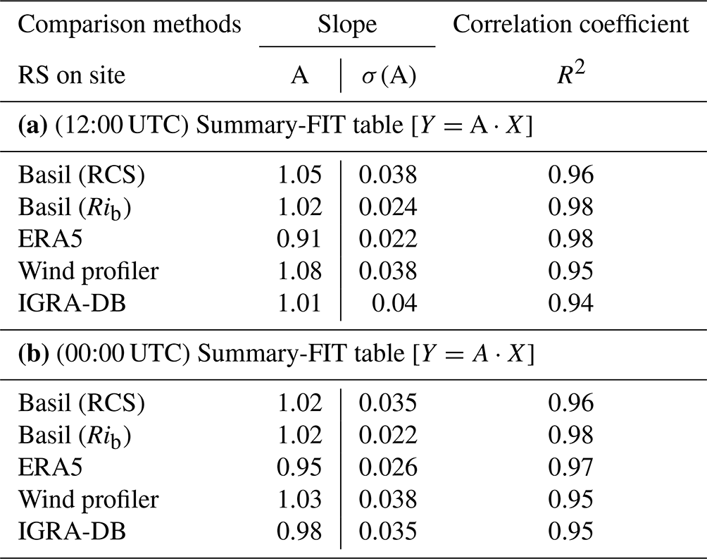
More specifically, Fig. 3a1 compares the reference daytime ABLH estimates with those obtained through the Richardson number method applied to the Raman lidar data, with R2 being equal to 0.98 and slope being equal to 1.02. This result confirms the small bias (2 %) affecting ABLH estimates from the Raman lidar data when compared with the reference estimates. Identical values of R2 and slope are found in the night-time comparison (Fig. 3a2). Figure 3b1 compares the reference daytime ABLH estimates with those obtained through the Richardson number method applied to the IGRA radiosonde data, with R2 being equal to 0.94 and slope being equal to 1.01. This result confirms a very small bias (1 %) affecting ABLH estimates from the IGRA radiosonde data when compared with the reference estimates. Very similar values of R2 and slope, 0.95 and 0.98, respectively, are found in the night-time comparison (Fig. 3b2). Figure 3c1 compares the reference daytime ABLH estimates with those obtained through the Richardson number method applied to the ECMWF-ERA5 analysis data, with R2 being equal to 0.98 and slope being equal to 0.91. This result testifies to a small bias (9 %) affecting the ABLH estimate from the ECMWF-ERA5 analysis data when compared with the reference estimate. Values of R2 and slope for the night-time comparisons are 0.97 and 0.95, respectively (Fig. 3c2), which confirm the presence of a slightly smaller bias at night with respect to daytime. Figure 3d1 compares daytime ABLH estimates from the wind profiler with the reference ABLH values, with R2 being equal to 0.95 and slope being equal to 1.08. This result confirms a small bias (8 %) affecting the ABLH estimate from the wind profiler when compared with the reference estimate. Values of R2 and slope for the night-time comparison are 0.95 and 1.03, respectively (Fig. 3d2), which testifies to the presence of a slightly smaller bias at night with respect to daytime. Finally, Fig. 3e1 compares daytime ABLH estimates obtained from range-corrected elastic backscatter lidar signals with the reference ABLH values, with R2 being equal to 0.96 and slope being equal to 1.05. This result confirms a small bias (5 %) affecting the ABLH estimate obtained from the range-corrected elastic backscatter lidar signals when compared with the reference estimate. Values of R2 and slope for the night-time comparison are 0.96 and 1.02, respectively (Fig. 3e2), which testify to the presence of a slightly smaller bias at night with respect to daytime.
Overall, results clearly reveal that absolute biases are smaller during the night than during the day. This is most probably due to the fact that night-time portions of the measurement records are typically characterized by higher stability conditions. However, percentage biases are typically larger during the night when the ABL may become very shallow. In fact, in the presence of shallow ABLs, ABLH values become comparable with the measurement uncertainty, and this makes percentage biases intrinsically high. In our specific case, ABLH values are found to not exceed 300 m throughout most parts of the month of October 2012. With a vertical resolution of 150 m, the uncertainty affecting the estimate of the ABLH is 50 % when sounding ABLs having heights not exceeding 300 m. As already anticipated above, the bias affecting the ABLH obtained from the range-corrected elastic backscatter lidar signals is possibly generated by the limited sensitivity of this sensor below 250 m as a result of the presence of overlap effects and a blind vertical region. Furthermore, the negative biases observed in ERA5 ABLH estimate are most probably associated with the negative bias affecting ERA5 water vapour and wind v component data.
The above results reveal that the different ABLH methods considered in the paper, which refer to different definitions and physical (dynamic and thermodynamic) processes, ultimately lead to ABLH estimates that are in very good agreement among them. This conclusion, which needs to be confirmed over longer time series including a complete seasonal cycle, confirms that turbulent air motion and vertical mixing, induced by shear and buoyancy forces (Stull, 1988), cause rapid fluctuations of several physical quantities, such as flow velocity, temperature, moisture and aerosol concentration, which are strongly correlated with each other. This result confirms the correctness of the considered approach to simultaneously apply different ABLH estimation methods which refer to the variability in different physical quantities.
Additional parameters from ERA5 reanalysis data have been considered to corroborate the interpretation of the observed atmospheric features. Figure 4 shows the time evolution of the convective available potential energy (CAPE; panel a), the friction velocity (panel b) and the relative humidity (panel c) from ERA5 reanalysis over the time period 1–31 October 2012. Friction velocity quantifies the vertical transport of momentum, or turbulence generation. It is calculated as the square root of the surface stress divided by air density. Friction velocity includes both a turbulent and a viscous component. In a turbulent flow, friction velocity is approximately constant within the few lowest metres of the atmosphere. This parameter increases with surface roughness. CAPE quantifies atmospheric instability (i.e. work done by the buoyancy on the air mass), with large positive values (>400) being necessary for the onset of convective activity in a conditionally unstable tropospheric layer. CAPE is strongly controlled by the ABL properties, with their coupling holding in both convective and non-convective conditions (Donner and Phillips, 2003). Additionally, the response of the boundary layer to near-surface (or 2 m) relative humidity is investigated, although it is known that it involves competing mechanisms (Ek and Mahrt, 1994) and the net effect of relative humidity is difficult to disentangle. Nevertheless, in the literature, the effect of relative humidity on the ABLH and its variability is often investigated because, in general, the ABLH is higher for high surface temperature and low humidity values, which translates into surface sensible heat fluxes dominating over latent heat fluxes and leading to increased buoyancy (Zhang et al., 2013).
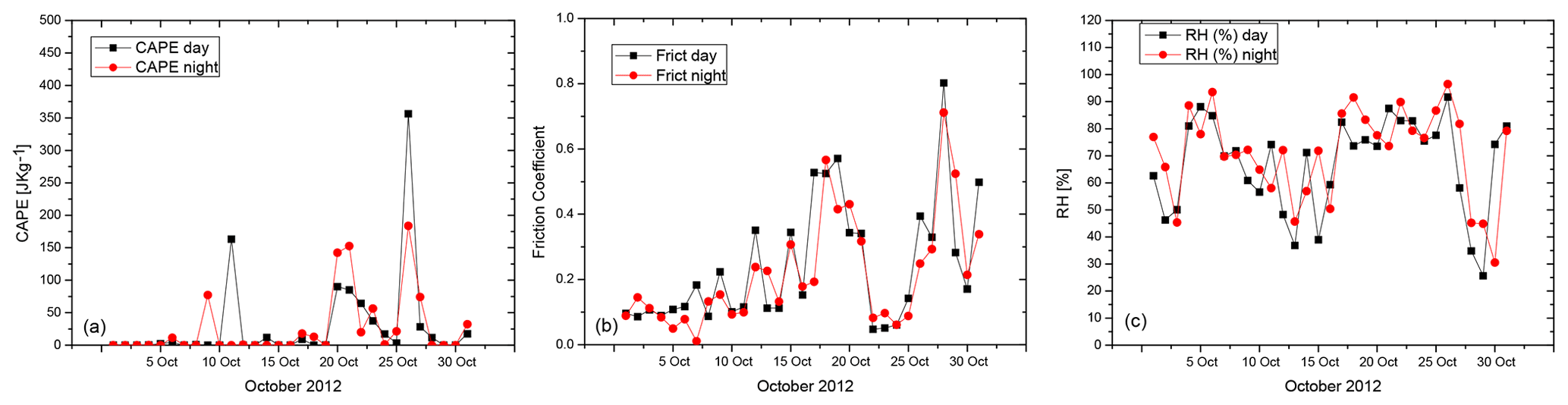
Figure 4ERA5 atmospheric reanalysis for CAPE (a). Friction velocity (b) and relative humidity (c) for the month of October 2012. Results are reported for both daytime (black lines, 12:00 UTC) and night-time (red lines, 00:00 UTC) comparisons.
Peak values in friction velocity are found in association with the highest ABLH values. During the month of October 2012 this happens around 18–19 October. This result confirms the important role played by the vertical transport of momentum and turbulence in the development of the ABL and in ABLH growth. CAPE values in excess of 100 J kg−1 are observed in the time periods 9–11, 19–21 and 25–27 October 2012, but no evident correlation is found with the corresponding time evolution of the ABLH. Within all other periods CAPE values are in the range 50–100 J kg−1, which are indicative of high-stability conditions and of an atmospheric environment unfavourable to convective activity on these days. Relative humidity values are found to experience a large variability, but no clear correlation appear to be present with ABLH estimates. The correlation between relative humidity and ABLH was verified in order to assess the potential role of water vapour in feeding convective activity and consequently in determining an increase in the ABLH when triggering mechanisms are present.
The above results reveal the role of atmospheric stability in limiting the ABLH variability. The high stability present during most of the month of October is probably one of the main drivers of the very good correlation found between the different sensors, models and methods. Figure 5 illustrates the percentage bias of the different ABLH estimates with respect to the reference one, expressed as a function of the atmospheric stability conditions. The presence of stable or unstable conditions was verified based on the use of the “lifted index” obtained from ERA5 model analysis data, with negative values for this index indicating instability – the higher the negative values in the index are, the more unstable the air is – and positive values indicating stability. More than 50 % of the cases can be classified as stable conditions, while the remaining cases can be classified as unstable. For the unstable conditions mutual deviations between the different sensors and methods are approximately 30 % larger than in the case of stable conditions. A lower dispersion of the bias values implies a higher correlation among the different ABLH estimates in the case of stable weather conditions.
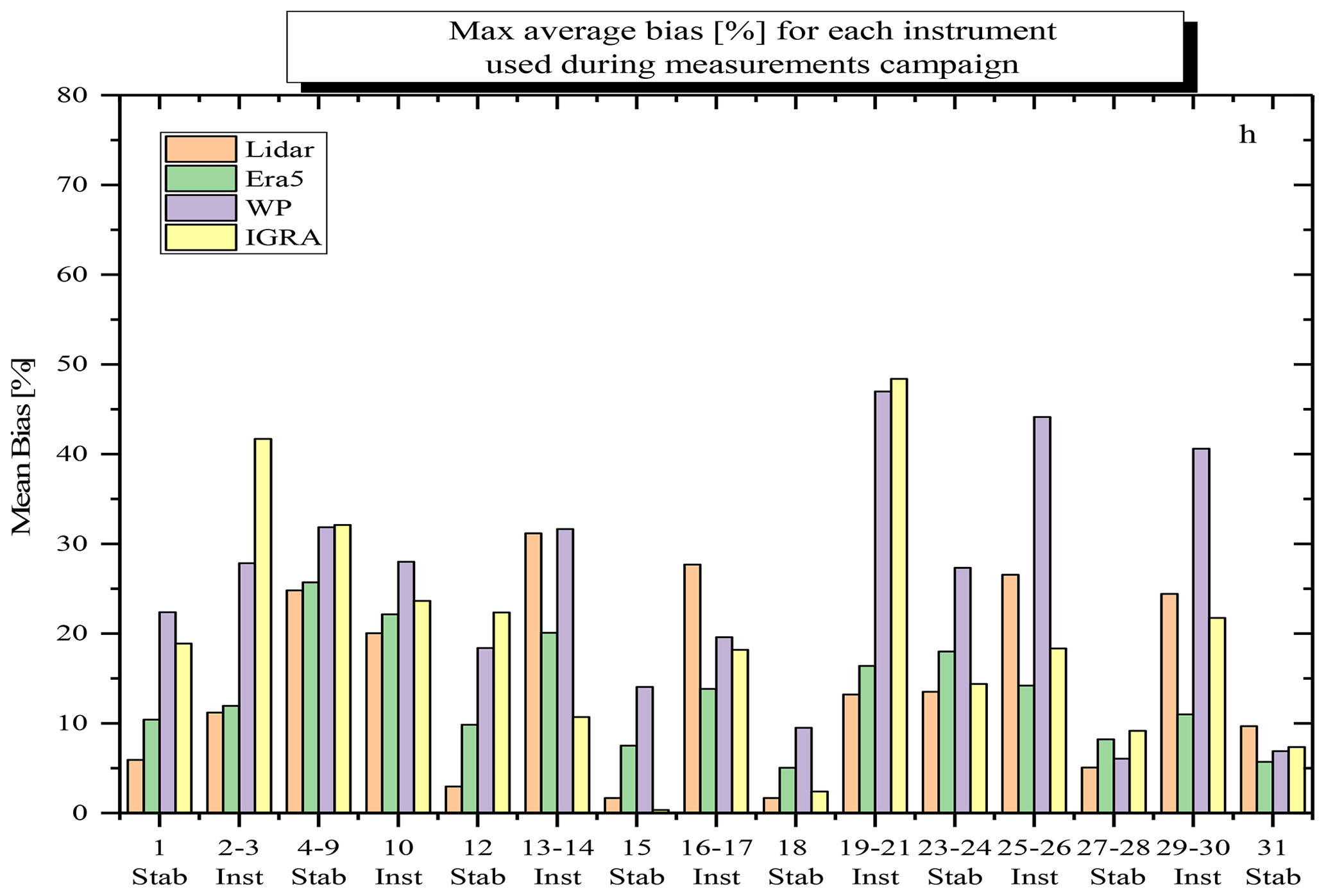
Figure 5Percentage bias of the different ABLH estimates with respect to the one obtained through the application of the Richardson number approach to the on-site radiosonde profiles, expressed as a function of the atmospheric stability conditions.
We also tried to quantitatively correlate ABLH estimates with the variability in CAPE, friction velocity and relative humidity. A linear fit was applied to the time series of the CAPE day-by-day gradient, the friction velocity and the relative humidity values in the time period 1–31 October 2012 vs. the corresponding ABLH estimates (plots not shown here). The correlation between ABLH estimates and the corresponding CAPE day-by-day gradient values is found to be characterized by a correlation coefficient of 0.51 in daytime and 0.46 at night; the correlation between ABLH estimates and the corresponding friction velocity values is found to be characterized by a correlation coefficient of 0.75 in daytime and 0.91 at night; finally, the correlation between ABLH estimates and the corresponding relative humidity values is found to be characterized by a correlation coefficient of 0.41 in daytime and 0.45 at night. These results reveal a reasonably good correlation between ABLH estimates and corresponding friction velocity values and a mild correlation between ABLH estimates and corresponding CAPE day-by-day gradient and relative humidity values. In order to further underline the correlation between ABLH estimates and corresponding friction velocity values, a scatter plot of ABLH vs. friction velocity for the month of October 2012 is illustrated in Fig. 6. In order to more easily reveal the higher correlation during night-time, data points are plotted separately for daytime (red dots, 12:00 UTC) and night-time (black dots, 00:00 UTC).
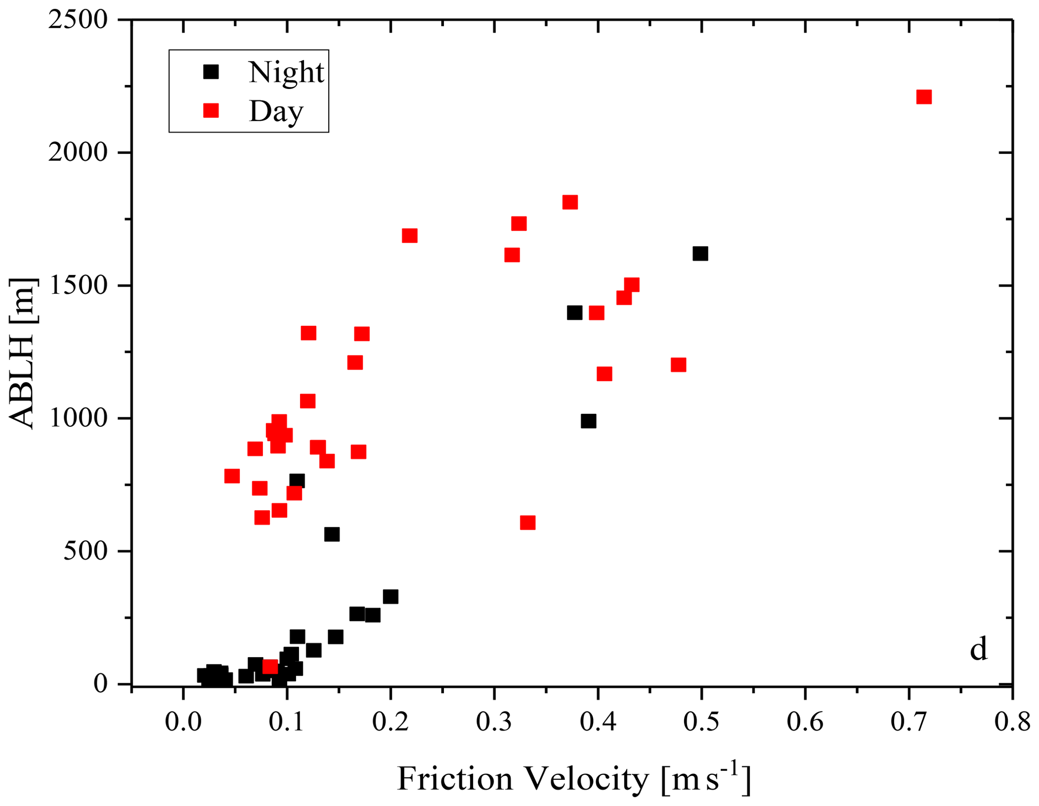
Figure 6Scatter plot of ABLH vs. friction velocity for the month of October 2012. Results are reported for both daytime (red dots, 12:00 UTC) and night-time (black dots, 00:00 UTC).
4.2 Short-term variability over the 2 d period of 18 and 19 October 2012
For the purpose of assessing the performance in monitoring the short-term variability in the ABLH, our analysis was also focused on one specific extended case study, covering the two complete daily cycles on 18 and 19 October 2012 and the night in between. Figure 7a illustrates the time–height cross section of the range-corrected signals (RCSs) at 355 nm as measured by BASIL over the time interval from 09:00 UTC on 18 October 2012 to 19:00 UTC on 19 October 2012. The figure includes approximately 400 consecutive RCS profiles, each one integrated over a time interval of 5 min and with a vertical resolution of 150 m. The six ABLH estimates are also included in the figure, with different symbols being used to identify the different ABLH sensors, models and approaches.
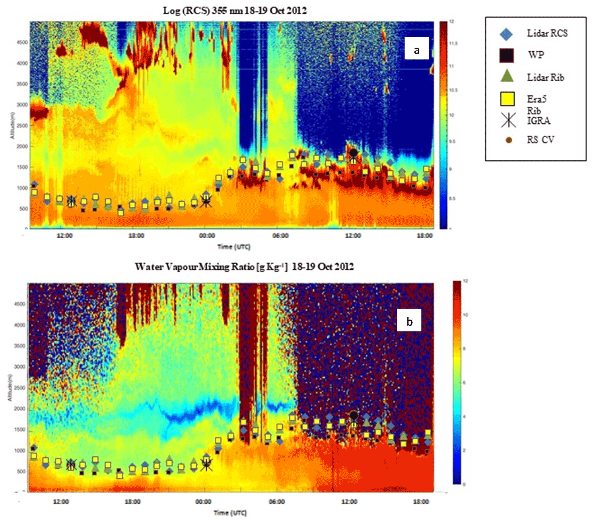
Figure 7(a) Time–height cross section of the range-corrected signals (RCSs) at 355 nm and (b) water vapour mixing ratio as measured by BASIL over the time interval from 23:00 UTC on 18 October 2012 to 19:00 UTC on 19 October 2012. The figure also includes the different ABL estimates.
This measurement period is characterized by variable weather conditions, which translate into variable aerosol and water vapour concentrations at different altitudes, with the presence of both surface and elevated aerosol and humidity layers. Such conditions are ideal to assess the performance of the different sensors, models and approaches and their capability to resolve the short-term variability in the ABLH. Specifically, on 18 October 2012 an elevated mesoscale convective system (MCS) is found to transit over the lidar station, with the cloud system base ranging between 2.5 and 4.5 km. Light precipitation is observed around 11:00 and 12:00 UTC, while virga events, with precipitating particles sublimating before reaching the ground, are observed later in the afternoon in the time interval 17:00–19:00 UTC. On 18 October 2012 the ABLH is found to descend from an initial value of 0.8–1.0 km around 09:30 UTC down to a minimum of 0.5–0.7 km around 18:00 UTC and then keep almost constant until 23:30 UTC. The limited growth of the ABLH on 18 October is probably associated with the shading effect of clouds, which prevent an effective onset of convective activity. Stratiform clouds are found to transit over the lidar site in the time interval 02:00–05:00 UTC on 19 October, with strong evidence of them in the RCSs (cloud base is at 1.0–1.2 km, and vertical extent is ∼0.2 km). Starting around 07:00 UTC on 19 October stratiform clouds are continuously present throughout the day, with a cloud base progressively descending from ∼1.4 to ∼0.8 km. Evidence of shallow orographic stratiform precipitation is also observed throughout the day. All ABLH estimates indicate a marked increase around 00:00 UTC on 19 October, with values rising from 0.5–0.7 up to 1.1–1.3 km. Such abrupt increase in ABLH is probably associated with the observed changes in the wind field flow, with the wind direction turning from east to north and the wind speed decreasing from ∼20 kn down to 3–5 kn, and the consequent change in sounded air masses. This change in the ABL structure is caused by advection of air masses with different thermodynamic and compositional properties associated with the wind direction turning, ultimately altering the stability and turbulent state of the sounded air masses. A similar abrupt ABLH variability had been reported by Pal and Lee (2019), who revealed the important role played in coastal areas by advection via onshore and offshore flows. All six ABLH estimates are coherent in revealing this abrupt ABLH increase.
Coming to the specific details of the comparison between the different ABLH estimates, throughout the day on 18 October the six estimates are all in very good agreement, with values always within 200 m one from the other, except for a few data points. Throughout the day on 19 October, despite the potential issues/problems associated the with the presence of the thick stratiform clouds and light precipitation, all six ABLH estimates are in reasonably good agreement, with all values within 200–300 m. On 19 October ABLH estimates from the wind profiler are systematically found to be slightly smaller than all other estimates. The slightly larger bias characterizing the wind profiler with respect to the other ABLH estimates was already underlined above when focusing on the climatological analysis throughout the month of October 2012. None of the six ABLH estimates appears to be affected by the presence of the thick stratiform clouds, not even the estimates based on the use of the elastic backscatter signals.
Figure 7b illustrates the time–height cross section of the water vapour mixing ratio measurements carried out by BASIL on the same day, which are displayed over the same time interval considered in Fig. 7a. A dry layer appears at the ABL top throughout most parts of the day on 18 October, probably resulting from sub-cloud low-level rain evaporation. This dry layer may ultimately have contributed to convection regeneration events observed throughout the passage of the MCS (Li et al., 2009; Morrison et al., 2009). It is to be specified that rain evaporation significantly contributes to the heat and moisture budgets of clouds (Emanuel et al., 1994), but few observations of these processes are available (Gamache et al., 1993). Dry layers are frequently observed in mid-latitude convective environments as a result of air being advected from different source regions under directionally sheared vertical wind profiles (Carlson and Ludlam, 1968). Deep convective precipitation events are influenced, and frequently favoured, by the presence of aerosols and mid-level dry layers, and this circumstance may have played a significant role in the formation and development of the observed MCS on this day.
In the present paper we illustrate and discuss the results from an inter-comparison effort considering ABL height estimates obtained from different sensors, models and techniques. The effort was carried out in the framework of HyMeX-SOP1. ABLH estimates were obtained using the Richardson number technique to Raman lidar and radiosonde measurements and to ECMWF-ERA5 reanalysis data. The inter-comparison also includes ABLH measurements from the wind profiler, which rely on the turbulence method, as well as measurements obtained from elastic backscatter lidar signals. A climatological assessment focusing on the evolution of the ABL height throughout the duration of the month of October 2012 was provided, with the inter-comparison being extended to both daytime and night-time data.
In the inter-comparison effort the Richardson number approach applied to the on-site radiosonde data is taken as reference. Results reveal a good agreement between the different datasets and approaches, all of them being able to capture the major features of ABLH time evolutions. Values of the correlation coefficient R2 are in the range 0.94–0.98. Biases of the single ABLH estimates with respect to the reference ABLH values were also determined through both a simple statistical analysis (mean deviation between the single sensor and model values and the reference values) and a regression analysis (slope of the linear fit regression line correlating the single sensor and model values and the reference values), with all bias values being smaller that 9 % in daytime and smaller than 5 % at night. The analysis was integrated with the comparison with a variety of atmospheric dynamic and thermodynamic variables from ERA5, namely convective available potential energy, friction velocity and relative humidity, with friction velocity found to be one of the main drivers of the ABLH variability.
The analysis was also focused on one specific case study, covering an extended time interval from 09:00 UTC on 18 October 2012 to 19:00 UTC on 19 October 2012, including two daytime portions, the first one characterized by the presence of high scattered clouds between 3 and 4 km and the second one characterized by the presence of low stratiform clouds between 1 and 2 km, which allowed us to assess the performance in the characterization of the short-term variability in the ABLH in variable weather conditions. This final analysis, while providing encouraging preliminary results, can to no extent be considered a thorough demonstration of the applicability of the considered approaches to variable complex weather conditions as in fact a more comprehensive and extensive study has to be carried out in the future in this direction.
The procedures and algorithms used in this research effort are properly described throughout the paper. Calculations and graphics have been developed with our own developed routines coded in MATLAB and C++. For further information write to donato.summa@imaa.cnr.it.
The data considered in the paper are accessible through the following repositories: https://www.hymex.org/ (last access: 25 July 2021; HyMeX, 2021) and https://www.ncei.noaa.gov/products/weather-balloon/integrated-global-radiosonde-archive (last access: 16 June 2021; NOAA NCEI, 2021).
All authors collaborated and contributed to drafting, reviewing and editing the paper. In particular, PDG and DS coordinated the effort and wrote the original draft. FM, NF and BDR contributed to the reviewing of the data analysis algorithms, the data analysis and the paper.
The contact author has declared that neither they nor their co-authors have any competing interests.
Publisher’s note: Copernicus Publications remains neutral with regard to jurisdictional claims in published maps and institutional affiliations.
This article is part of the special issue “Hydrological cycle in the Mediterranean (ACP/AMT/GMD/HESS/NHESS/OS inter-journal SI)”. It is not associated with a conference.
Wind profiler datasets were obtained from the HyMeX programme, sponsored by grants MISTRALS/HyMeX and ANR-11-BS56-0005 IODA-MED project (contact person: Said Frèdèrique Laboratoire d'Aérologie, Université de Toulouse, UMR CNRS 5560).
This research has been supported by the French National Research Agency (ANR) (grant nos. MISTRALS/HyMeX and ANR-11-BS56-0005 IODA-MED project), the Italian Ministry for Education, University and Research (grants STAC-UP and FISR2019-CONCERNING), and the Italian Space Agency (grants As-ATLAS and CALIGOLA).
This paper was edited by Domenico Cimini and reviewed by two anonymous referees.
Behrendt, A., Pal, S., Aoshima, F., Bender, M., Blyth, A., Corsmeier, U., Cuesta, J., Dick, G., Dorninger, M., Flamant, C., Di Girolamo, P., Gorgas, T., Huang, Y., Kalthoff, N., Khodayar, S., Mannstein, H., and Wulfmeyer, V.: Observation of Convection Initiation Processes with a Suite of State-of-the-Art Research Instruments during COPS IOP8b, Q. J. Roy. Meteor. Soc., 137, 81–100, https://doi.org/10.1002/qj.758, 2011.
Bhawar, R., Di Girolamo, P., Summa, D., Flamant, C., Althausen, D., Behrendt, A., Kiemle, C., Bosser, P., Cacciani, M., Champollion, C., Di Iorio, T., Engelmann, R., Herold, C., Müller, D., Pal, S., Wirth, M., and Wulfmeyer, V.: The Water Vapour Intercomparison Effort in the Framework of the Convective and Orographically-Induced Precipitation Study: Airborne-to-Ground-based and airborne-to-airborne Lidar Systems, Q. J. Roy. Meteor. Soc., 137, 325–348, https://doi.org/10.1002/qj.697, 2011.
Bianco, L. and Wilczak, J. M.: Convective boundary layer depth: improved measurement by Doppler radar wind profiler using fuzzy logic methods, J. Atmos. Ocean. Tech., 19, 1745–1758, 2002.
Carlson, T. N. and Ludlam, F. H.: Conditions for the occurrence of severe local storms, Tellus A, 20, 203–226, https://doi.org/10.1111/j.2153-3490.1968.tb00364.x, 1968.
Che, J. and Zhao, P.: Characteristics of the summer atmospheric boundary layer height over the Tibetan Plateau and influential factors, Atmos. Chem. Phys., 21, 5253–5268, https://doi.org/10.5194/acp-21-5253-2021, 2021.
Cramer, O. P.: Potential temperature analysis for mountainous terrain, J. Appl. Meteorol., 11, 44–50, 1972.
Dai, C., Wang, Q., Kalogiros, J. A., Lenschow, D. H., Gao, Z., and Zhou, M.: Determining Boundary-Layer Height from Aircraft Measurements, Bound.-Lay. Meteorol., 152, 277–302, https://doi.org/10.1007/s10546-014-9929-z, 2014.
Dai, H., Katherine, K., Milkman, L., and Riis, J.: The Fresh Start Effect: Temporal Landmarks Motivate Aspirational Behavior, Manage. Sci., 60, 2563–2582, https://doi.org/10.1287/mnsc.2014.1901, 2014.
Dang, R., Yang, Y., Li, H., Hu, X.-M., Wang, Z., Huang, Z., Zhou, T., and Zhang, T.: Atmosphere Boundary Layer Height (ABLH) Determination under Multiple-Layer Conditions Using Micro-Pulse Lidar, Remote Sens., 11, 263, https://doi.org/10.3390/rs11030263, 2019a.
Dang, R., Yang, Y., Hu, X.-M., Wang, Z., and Zhang, S. A.: Review of Techniques for Diagnosing the Atmospheric Boundary Layer Height (ABLH) Using Aerosol Lidar Data, Remote Sens., 11, 1590, https://doi.org/10.3390/rs11131590, 2019b.
Dee, D. P., Fasullo, J., Shea, D., Walsh, J., and National Center for Atmospheric Research Staff (Eds.): The climate data guide: Atmospheric reanalysis: Overview and comparison tables, NCAR https://climatedataguide.ucar.edu/climate-data/atmospheric-reanalysis-overview-comparison-tables (last access: 12 June 2021), 2016.
De Wekker, S. F. J., Kossmann, M., and Fielder, F.: Observations of daytime mixed layer heights over mountainous terrain during the TRACT field campaign, in: Proc. 12th Symp. on Boundary Layers and Turbulence, Vancouver, BC, Canada, 28 July–1 August 1997, Am. Meteor. Soc., 1, 498–499, 1997.
Di Girolamo, P., Marchese, R., Whiteman, D. N., and Demoz, B. B.: Rotational Raman Lidar measurements of atmospheric temperature in the UV, Geophys. Res. Lett., 31, L01106, https://doi.org/10.1029/2003GL018342, 2004.
Di Girolamo, P., Summa, D., and Ferretti, R.: Multiparameter Raman Lidar Measurements for the Characterization of a Dry Stratospheric Intrusion Event, J. Atmos. Ocean. Tech., 26, 1742–1762, https://doi.org/10.1175/2009JTECHA1253.1, 2009a.
Di Girolamo, P., Summa, D., Lin, R.-F., Maestri, T., Rizzi, R., and Masiello, G.: UV Raman lidar measurements of relative humidity for the characterization of cirrus cloud microphysical properties, Atmos. Chem. Phys., 9, 8799–8811, https://doi.org/10.5194/acp-9-8799-2009, 2009b.
Di Girolamo, P., Summa, D., Bhawar, R., Di Iorio, T., Cacciani, M., Veselovskii, I., Dubovik, O., and Kolgotin, A.: Raman lidar observations of a Saharan dust outbreak event: characterization of the dust optical properties and determination of particle size and microphysical parameters, Atmos. Environ., 50, 66–78, https://doi.org/10.1016/j.atmosenv.2011.12.061, 2012a.
Di Girolamo, P., Summa, D., Cacciani, M., Norton, E. G., Peters, G., and Dufournet, Y.: Lidar and radar measurements of the melting layer: observations of dark and bright band phenomena, Atmos. Chem. Phys., 12, 4143–4157, https://doi.org/10.5194/acp-12-4143-2012, 2012b.
Di Girolamo, P., Flamant, C., Cacciani, M., Richard, E., Ducrocq, V., Summa, D., Stelitano, D., Fourrié, N., and Saïd, F.: Observation of low-level wind reversals in the Gulf of Lion area and their impact on the water vapour variability, Q. J. Roy. Meteor. Soc., 142, 153–172, https://doi.org/10.1002/qj.2767, 2016.
Di Girolamo, P., Cacciani, M., Summa, D., Scoccione, A., De Rosa, B., Behrendt, A., and Wulfmeyer, V.: Characterisation of boundary layer turbulent processes by the Raman lidar BASIL in the frame of HD(CP)2 Observational Prototype Experiment, Atmos. Chem. Phys., 17, 745–767, https://doi.org/10.5194/acp-17-745-2017, 2017.
Donner, L. J. and Phillips, V. T.: Boundary layer control on convective available potential energy: Implications for cumulus parameterization, J. Geophys. Res., 108, 4701, https://doi.org/10.1029/2003JD003773, 2003.
Durré, I., Yin, X., Vose, R. S., Applequist, S., and Arnfield, J.: Enhancing the Data Coverage in the Integrated Global Radiosonde Archive, J. Atmos. Ocean. Tech., 35, 1753–1770, 2018.
Emanuel, K. A., Neelin, J. D., and Bretherton, C. S.: On large-scale circulations in convecting atmospheres, Q. J. Roy. Meteor. Soc., 120, 1111–1143, 1994.
Ek, M. and Mahrt, L.: Daytime Evolution of Relative Humidity at the Boundary Layer Top, Mon. Weather Rev., 122, 2709–2721, https://doi.org/10.1175/1520-0493(1994)122<2709:DEORHA>2.0.CO;2, 1994.
Esau, I. and Zilitinkevich, S.: On the role of the planetary boundary layer depth in the climate system, Adv. Sci. Res., 4, 63–69, https://doi.org/10.5194/asr-4-63-2010, 2010.
Gage, K. S., Balsley, B. B., Ecklund, W. L., Woodman, R. F., and Avery, S. K.: Wind-profiling Doppler radars for tropical atmosphericresearch, Eos T. AGU, 71, 1851–1854, 1990.
Gamache, J. F., Houze, R. A., Marks, F. D.: Dual-aircraft investigation of the inner core of hurricane Norbert. 3. Water-budget, J. Atmos. Sci., 50, 3221–3243, 1993.
Garratt, J.: Review: The atmospheric boundary layer, Earth Sci. Rev., 37, 89–134, 1994.
Garratt, J. R.: The Atmospheric Boundary Layer, Cambridge Atmospheric and Space Science Series, Cambridge Univ. Press, 335 pp., ISBN 0-521-38052-9, 1992.
Haeffelin, M., Angelini, F., Morille, Y., Martucci, G., O'Dowd, C. D., Xueref-Rémy, I., Wastine, B., Frey, S., and Sauvage, L.: Evaluation of mixing depth retrievals from automatic profiling lidars and ceilometers inview of future integrated networks in Europe, Bound.-Lay. Meteorol., 143, 49–75, https://doi.org/10.1007/s10546-011-9643-z, 2012.
Hanna, S. R.: The thickness of the planetary boundary layer, Atmos. Environ., 3, 519–536, https://doi.org/10.1016/0004-6981(69)90042-0, 1969.
Herrera-Mejía, L. and Hoyos, C. D.: Characterization of the atmospheric boundary layer in a narrow tropical valley using remote-sensing and radiosonde observations and the WRF model: the Aburrá Valley case-study, Q. J. Roy. Meteor. Soc., 145, 2641–2665, https://doi.org/10.1002/qj.3583, 2019.
Hersbach, H., Bell, B., Berrisford P., Hirahara S., Horányi, A., Muñoz-Sabater, J., Nicolas, J., Peubey, C., Radu, R., Schepers, D., Simmons, A., Soci, C., Abdalla, S., Abellan, X., Balsamo, G., Bechtold, P., Biavati, G., Bidlot, J., Bonavita, M., De Chiara, G., Dahlgren, P., Dee, D., Diamantakis, M., Dragani, R., Flemming, J., Forbes, R., Fuentes, M., Geer, A., Haimberger, L., Healy, S., Robin J., Hogan, R.J., Hólm, E., Janisková, M., Keeley, S., Laloyaux, P., Lopez, P., Lupu, C., Radnoti, G., De Rosnay, P., Rozum, I., Vamborg, F., Villaume, S., and Thépaut J.-N.: The ERA5 reanalysis, Q. J. Roy. Meteor. Soc., 146, 1999–2049, https://doi.org/10.1002/qj.3803, 2020.
HyMeX: https://www.hymex.org/, last access: 25 July 2021.
Hyun, Y., Kim, K.-E., and Ha, K.-J.: A comparison of methods to estimate the height of stable boundary layer over a temperate grassland, Agr. Forest Meteorol., 132, 132–142, 2005.
Jericevic, A. and Grisogono, B.: The critical bulk Richardson number in urban areas: verification with application in NWP model, Tellus A, 58, 19–27, https://doi.org/10.3402/tellusa.v58i1.14743, 2006.
Joffre, S. M., Kangas, M., Heikinheimo, M., and Kitaigorodskii, S. A.: Variability of the stable and unstable atmospheric boundary-layer height and its scales over a boreal forest, Bound.-Lay. Meteorol., 99, 429–450, 2001.
Lenschow, D. H., Zhou, M., Zeng, X., Chen, L., and Xu, X.: Measurements of fine-scale structure at the top ofmarine stratocumulus, Bound.-Lay. Meteorol., 97, 331–357, 2000.
Li, J., Carlson, B. E., and Lacis, A. A.: A study on the temporal and spatial variability of absorbing aerosols using total ozone mapping spectrometer and ozone monitoring instrument aerosol index data, J. Geophys. Res., 114, D09213, https://doi.org/10.1029/2008JD011278, 2009.
Liu, Z., Chang, J., Li, H., Chen, S., and Dai, T.: Estimating Boundary Layer Height from LiDAR Dataunder Complex AtmosphericConditions Using Machine Learning, Remote Sens., 14, 418, https://doi.org/10.3390/rs14020418, 2022.
Madonna, F., Kivi, R., Dupont, J.-C., Ingleby, B., Fujiwara, M., Romanens, G., Hernandez, M., Calbet, X., Rosoldi, M., Giunta, A., Karppinen, T., Iwabuchi, M., Hoshino, S., von Rohden, C., and Thorne, P. W.: Use of automatic radiosonde launchers to measure temperature and humidity profiles from the GRUAN perspective, Atmos. Meas. Tech., 13, 3621–3649, https://doi.org/10.5194/amt-13-3621-2020, 2020.
Madonna, F., Summa, D., Di Girolamo, P., Marra, F., Wang, Y., and Rosoldi, M.: Assessment of Trends and Uncertainties in the Atmospheric Boundary Layer Height Estimated Using Radiosounding Observations over Europe, Atmosphere, 12, 301, https://doi.org/10.3390/atmos12030301, 2021.
Manninen, A. J., Marke, T., Tuononen, M. J., and O'Connor, E. J.: Atmospheric boundary layer classification with Doppler lidar, J. Geophys. Res.-Atmos., 123, 8172–8189, https://doi.org/10.1029/2017JD028169, 2018.
Martucci, G., Matthey, R., and Mitev, V.: Comparison between backscatter lidar and radiosonde measurements of the diurnal and nocturnal stratification in the lower troposphere, J. Atmos. Ocean. Tech., 24, 1231–1244, 2007.
Melgarejo, J. W. and Deardorff, J. W.: Stability functions for the boundary layer resistance laws based upon observed boundary-layer heights, J. Atmos. Sci., 31, 1324–1333, 1974.
Morrison, H. G., Thompson, G., and Tatarskii, V.: Impact of cloud microphysics on the development of trailing stratiform precipitation in a simulated squall line: Comparison of one and two-moment schemes, Mon. Weather Rev., 137, 991–1007, https://doi.org/10.1175/2008MWR2556.1, 2009.
Nash, J., Oakley, T., Vömel, H., and Wei, L.: WMO intercomparison of high quality radiosonde systems, Yangjiang, China, 12 July–3 August 2010, World Meteorological Organization (WMO), WMO/TD-No. 1580, 2010.
NOAA NCEI: Integrated Global Radiosonde Archive (IGRA), https://www.ncei.noaa.gov/products/weather-balloon/integrated-global-radiosonde-archive, last access: 16 June 2021.
Oke, T. R.: Boundary Layer Climates, 2nd edn., Halsted Press, New York, 435 pp., 1988.
Pal, S. and Lee, T. R.: Contrasting air mass advection explains significant differences in boundary layer depth seasonal cycles under onshore versus offshore flows, Geophys. Res. Lett., 46, 2846–2853, https://doi.org/10.1029/2018GL081699, 2019.
Saïd, F., Campistron, B., Delbarre, H., Canut, G., Doerenbecher,A., Durand, P., Fourrié, N., Lambert, D., and Legain, D.: Offshorewinds obtained from a network of wind-profiler radars duringHyMeX: 3D Wind Fields during HyMeX, Q. J. Roy. Meteor. Soc., 142, 23–42, https://doi.org/10.1002/qj.2749, 2016.
Saïd, F., Campistron, B., and Di Girolamo, P.: High-resolution humidity profiles retrieved from wind profiler radar measurements, Atmos. Meas. Tech., 11, 1669–1688, https://doi.org/10.5194/amt-11-1669-2018, 2018.
Seibert, P., Beyrich, F., Gryning, S.-E., Joffre, S., Rasmussen, A., and Tercier, P.: Review and intercomparison of operational methods for the determination of the mixing height, Atmos. Environ., 34, 1001–1027, https://doi.org/10.1016/S1352-2310(99)00349-0, 2000.
Seidel, D. J., Zhang, Y., Beljaars, A., Golaz, J.-C., Jacobson, A. R., and Medeiros, B.: Climatology of the planetary boundary layer over the continental United States and Europe, J. Geophys. Res., 117, D17106, https://doi.org/10.1029/2012JD018143, 2012.
Sicard, M., Pérez, C., Rocadenbosch, F., Baldasano, J. M., and García-Vizcaino, D.: Mixed-layer depth determination in the Barcelona coastal area from regular lidar measurements: methods, results and limitations, Bound.-Lay. Meteorol., 119, 135–157, 2006.
Sorbjan, Z.: Structure of the Atmospheric Boundary Layer, New Jersey, Prentice-Hall, 316 pp., ISBN-10: 0138535574, 1989.
Staudt, K.: Determination of the atmospheric boundary layer height in complex terrain during SALSA 2005, Dissertation thesis, Department of Micrometeorology, University of Bayreuth, September 2006.
Stelitano, D., Di Girolamo, P., Scoccione, A., Summa, D., and Cacciani, M.: Characterization of atmospheric aerosol optical properties based on the combined use of a ground-based Raman lidar and an airborne optical particle counter in the framework of the Hydrological Cycle in the Mediterranean Experiment – Special Observation Period 1, Atmos. Meas. Tech., 12, 2183–2199, https://doi.org/10.5194/amt-12-2183-2019, 2019.
Stull, R. B.: An Introduction to Boundary Layer Meteorology, Dordrecht, Kluwer, 666 pp., ISBN: 978-94-009-3027-8, 1998.
Summa, D., Di Girolamo, P., Stelitano, D., and Cacciani, M.: Characterization of the planetary boundary layer height and structure by Raman lidar: comparison of different approaches, Atmos. Meas. Tech., 6, 3515–3525, https://doi.org/10.5194/amt-6-3515-2013, 2013.
Van Pul, W. A. J., Holtslag, A. A. M., and Swart, D. P. J.: A comparison of ABL heights inferred routinely from lidar and radiosondes at noontime, Bound.-Lay. Meteorol., 68, 173–191, 1994.
Vivone, G., D'Amico, G., Summa, D., Lolli, S., Amodeo, A., Bortoli, D., and Pappalardo, G.: Atmospheric boundary layer height estimation from aerosol lidar: a new approach based on morphological image processing techniques, Atmos. Chem. Phys., 21, 4249–4265, https://doi.org/10.5194/acp-21-4249-2021, 2021.
Vogelezang, D. H. P. and Holtslag, A. A. M.: Evaluation and model impacts of alternative boundary-layer height formulations, Bound.-Lay. Meteorol., 81, 245–269, https://doi.org/10.1007/BF02430331, 1996.
Wang, Q., Lenschow, D. H., Pan, L., Schillawski, R. D., Kok, G. L., Prévot, A. S. H., Laursen, K., Russell, L. M., Bandy, A. R., Thornton, D. C., and Suhre, K.: Characteristics of the marine boundary layers during two Lagrangian measurements periods Turbolence structure, J. Geophys. Res., 104, 21767–21784, https://doi.org/10.1029/1998JD100100, 1999.
Zhang, Y., Seidel, D. J., and Zhang, S.: Trends in Planetary Boundary Layer Height over Europe, J. Climate, 26, 10071–10076, https://doi.org/10.1175/JCLI-D-13-00108.1, 2013.
Zhang, Y., Gao, Z., Li, D., Li, Y., Zhang, N., Zhao, X., and Chen, J.: On the computation of planetary boundary-layer height using the bulk Richardson number method, Geosci. Model Dev., 7, 2599–2611, https://doi.org/10.5194/gmd-7-2599-2014, 2014.
Zilitinkevich, S. and Baklanov, A.: Calculation Of The Height Of The Stable Boundary Layer In Practical Applications, Bound.-Lay. Meteorol., 105, 389–409, https://doi.org/10.1023/A:1020376832738, 2002.
- Abstract
- Introduction
- Methods considered for the determination of the ABLH
- Profiling sensors and model data involved in the inter-comparison effort
- Results
- Conclusions
- Code availability
- Data availability
- Author contributions
- Competing interests
- Disclaimer
- Special issue statement
- Acknowledgements
- Financial support
- Review statement
- References