the Creative Commons Attribution 4.0 License.
the Creative Commons Attribution 4.0 License.
 | 27 Sep 2022
A new machine-learning-based analysis for improving satellite-retrieved atmospheric composition data: OMI SO2 as an example
Joanna Joiner
Nickolay A. Krotkov
Vitali Fioletov
Chris McLinden
Despite recent progress, satellite retrievals of anthropogenic SO2 still suffer from relatively low signal-to-noise ratios. In this study, we demonstrate a new machine learning data analysis method to improve the quality of satellite SO2 products. In the absence of large ground-truth datasets for SO2, we start from SO2 slant column densities (SCDs) retrieved from the Ozone Monitoring Instrument (OMI) using a data-driven, physically based algorithm and calculate the ratio between the SCD and the root mean square (rms) of the fitting residuals for each pixel. To build the training data, we select presumably clean pixels with small SCD rms ratios (SRRs) and set their target SCDs to zero. For polluted pixels with relatively large SRRs, we set the target to the original retrieved SCDs. We then train neural networks (NNs) to reproduce the target SCDs using predictors including SRRs for individual pixels, solar zenith, viewing zenith and phase angles, scene reflectivity, and O3 column amounts, as well as the monthly mean SRRs. For data analysis, we employ two NNs: (1) one trained daily to produce analyzed SO2 SCDs for polluted pixels each day and (2) the other trained once every month to produce analyzed SCDs for less polluted pixels for the entire month. Test results for 2005 show that our method can significantly reduce noise and artifacts over background regions. Over polluted areas, the monthly mean NN-analyzed and original SCDs generally agree to within ±15 %, indicating that our method can retain SO2 signals in the original retrievals except for large volcanic eruptions. This is further confirmed by running both the NN-analyzed and original SCDs through a top-down emission algorithm to estimate the annual SO2 emissions for ∼500 anthropogenic sources, with the two datasets yielding similar results. We also explore two alternative approaches to the NN-based analysis method. In one, we employ a simple linear interpolation model to analyze the original SCD retrievals. In the other, we develop a PCA–NN algorithm that uses OMI measured radiances, transformed and dimension-reduced with a principal component analysis (PCA) technique, as inputs to NNs for SO2 SCD retrievals. While the linear model and the PCA–NN algorithm can reduce retrieval noise, they both underestimate SO2 over polluted areas. Overall, the results presented here demonstrate that our new data analysis method can significantly improve the quality of existing OMI SO2 retrievals. The method can potentially be adapted for other sensors and/or species and enhance the value of satellite data in air quality research and applications.
- Article
(14998 KB) - Full-text XML
-
Supplement
(15807 KB) - BibTeX
- EndNote


Sulfur dioxide (SO2) and its oxidation product in the atmosphere, sulfate aerosols, have significant impacts on air quality, visibility, ecosystems, and the weather and climate. For over 2 decades, spaceborne hyperspectral ultraviolet (UV) instruments (e.g., Eisinger and Burrows, 1998; Krotkov et al., 2006; Nowlan et al., 2011; Theys et al., 2017) have been providing global observations of anthropogenic SO2 sources such as coal-fired power plants, metal smelters, and the oil and gas industry (e.g., Fioletov et al., 2016; McLinden et al., 2016; Zhang et al., 2019). More recently, the quality of satellite SO2 data products has substantially improved thanks to the development of data-driven retrieval techniques. In particular, the algorithm based on principal component analysis (PCA) (Li et al., 2013, 2017a, 2020) and the covariance-based retrieval algorithm (COBRA, Theys et al., 2021) have helped to reduce the noise and artifacts of SO2 retrievals from several sensors including the Ozone Monitoring Instrument (OMI), Ozone Mapping and Profiler Suite (OMPS), and TROPOspheric Monitoring Instrument (TROPOMI), enabling the detection and quantification of relatively small point sources (e.g., Fioletov et al., 2015; Theys et al., 2021).
Despite these progresses, satellite remote sensing of anthropogenic SO2 remains challenging. The signal of anthropogenic SO2 is relatively weak compared with volcanic sources. With an atmospheric lifetime of ∼1 d (e.g., Lee et al., 2011), SO2 emitted from human activities is also more concentrated in the boundary layer, where the sensitivity of satellite instruments is limited by the low surface albedo, strong Rayleigh scattering, and interferences from O3 absorption in the UV (e.g., Krotkov et al., 2008). As a result, the noise in satellite SO2 retrievals is relatively large even for data-driven algorithms. For example, the standard deviation (1σ noise) of OMI PCA SO2 slant column densities (SCDs) over the remote Pacific is ∼ 0.2–0.3 DU (Dobson unit, 1 DU molecules cm−2, Li et al., 2020), which is far greater than the typical SCDs retrieved outside the most polluted areas (e.g., Persian Gulf, eastern China, and Norilsk, Russia). The retrieval noise can be reduced by spatially and temporally averaging the data (Krotkov et al., 2008). However, relatively small but noticeable artifacts still exist in monthly or annual mean OMI SO2 (e.g., negative values over arid and semi-arid areas), indicating systematic biases that cannot be averaged out. While there was little drift in the mean OMI SO2 SCDs over remote regions from 2005 to 2019, the retrieval noise grew by ∼10 % during the same period (Li et al., 2020), presumably due to instrument degradation. With the recent large decreases in SO2 emissions and signals in many regions (e.g., Krotkov et al., 2016; Li et al., 2017b), the increase in retrieval noise makes the analyses and applications of satellite SO2 data even more challenging, especially for long-term monitoring. It is thus imperative to further enhance the quality of satellite SO2 data products.
In recent years, machine learning has emerged as a powerful tool in satellite remote sensing of atmospheric composition. Capable of incorporating large, diverse datasets and modeling complex, nonlinear functions, techniques such as neural networks (NNs) and random forests (RFs) have been utilized to solve various problems. For instance, a number of studies trained NN or RF models to infer surface concentrations of pollutants from satellite observations, including particulate matter (e.g., Huang et al., 2021; Liu et al., 2019; Zheng et al., 2021), NO2 (e.g., Chan et al., 2021), and SO2 (e.g., Zhang et al. 2022). NNs have also been used to speed up radiative transfer calculations (e.g., Castellanos and da Silva, 2019; Nanda et al., 2019) and to retrieve O3 profiles (e.g., Müller et al., 2003; Xu et al., 2017) and total columns (Müller et al., 2004), isoprene amounts (Wells et al., 2020), and aerosol layer height (Chimot et al., 2017). For SO2, De Santis et al. (2021) demonstrated an NN retrieval algorithm using the operational TROPOMI product for training in their case study of Mt. Etna. Piscini et al. (2014) attempted NN-based SO2 and volcanic ash retrievals using thermal infrared measurements from MODIS (the Moderate Resolution Imaging Spectroradiometer). Hedelt et al. (2019) also developed near-real-time volcanic SO2 height retrievals using the full-physics inverse learning machine (FP-ILM) method, a technique later adapted for OMI by Fedkin et al. (2021). While these studies have demonstrated the potential of machine learning for SO2 retrievals, they all focus on volcanic SO2. To our knowledge, so far there have been no published studies demonstrating the use of machine learning techniques for anthropogenic SO2 retrievals.
A major obstacle in developing machine learning retrieval algorithms for anthropogenic SO2 is the lack of high-quality, ground-truth training data. As mentioned above, existing satellite SO2 products provide global coverage, but the signal-to-noise ratios are typically small for anthropogenic sources. Ground air quality monitors generally offer good data quality and long-term measurements, but they do not represent the entire atmospheric column. Aircraft measurements and surface-based remote sensing instruments (e.g., MAX-DOAS) have been used to evaluate satellite retrievals, but they are quite sparse. The FP-ILM method circumvents this data availability issue by using a large set of model-simulated synthetic radiance spectra in training. However, the models may not fully represent the various geophysical processes and instrument characteristics that affect satellite measurements. This can lead to substantial errors, and FP-ILM retrievals of volcanic SO2 height are currently limited to satellite pixels with sizable SO2 amounts (>20 DU).
Here, we introduce a new data analysis method to further improve the quality of satellite-retrieved SO2. In the absence of sufficient ground-truth data, we compile our training data by analyzing existing OMI SO2 SCD retrievals and the associated fitting errors, assuming that retrievals with greater SCDs and smaller fitting errors can be trusted more than those with smaller SCDs and larger errors. This allows us to train NNs to reduce noise and artifacts in the original retrievals while retaining SO2 signals over major emission source areas. The rest of the paper is organized as follows: Sect. 2 describes our methodology and setups for NN training. Section 3 provides some example results. This is followed by a more detailed discussion on the NN-analyzed SCDs in Sect. 4 and conclusions in Sect. 5.
The flowchart in Fig. 1a presents an overview of our data analysis method. We start from existing OMI PCA SO2 retrievals (Sect. 2.1) and calculate the ratio between the SCD and the root mean square (rms) of the fitting residuals (SCD rms ratio, SRR) for each pixel, as well as the statistics of the SRRs for the entire month. This provides input to a data classification scheme (Fig. 1b, Sect. 2.2) that assigns OMI pixels from each day into different groups (“clean”, “polluted”, “in between”, and “high SRR”). The pixels within each group are then either processed with one of the two neural networks (pre-trained NN1 for clean and in-between pixels, daily trained NN2 for polluted pixels; Fig. 1c, Sect. 2.3) or retain their original retrieved SCDs (for high-SRR pixels). In the end, the OMI pixels from different groups are merged into the final analyzed SCD dataset.
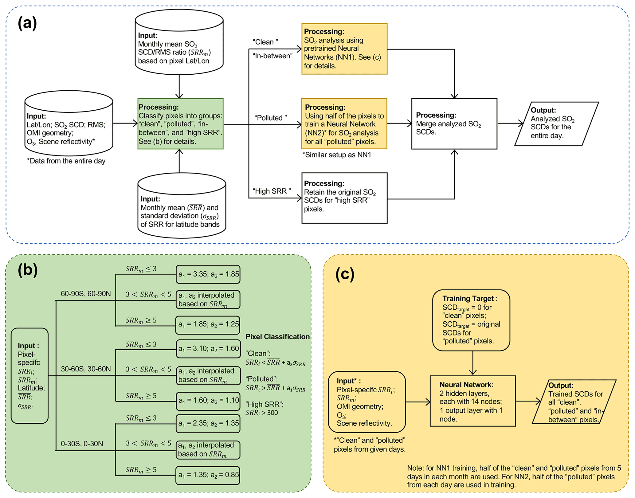
Figure 1(a) Flowchart of the SO2 analysis method. (b) Scheme for classification of OMI pixels as “clean”, “polluted”, “in between”, and “high SRR”. (c) Setups of the neural networks for SO2 SCD analysis.
2.1 Analysis of OMI SO2 data
To demonstrate our methodology, we use data from OMI, a Dutch–Finnish UV–visible spectrometer that has been flying on the National Aeronautics and Space Administration (NASA) Aura spacecraft in a Sun synchronous orbit since 2004 (Levelt et al., 2018). OMI measures backscattered solar radiation between 270 and 500 nm in the local afternoon (local Equator crossing time: ∼ 13:45) at a relatively high spatial (13×24 km2 at nadir) and spectral (∼0.5 nm) resolution. We focus on the year 2005, when all cross-track positions (rows) of OMI's two-dimensional detectors were taking nominal measurements, providing daily global coverage.
For SO2 data, we use SCDs retrieved from the NASA version 2 OMI standard SO2 algorithm based on the PCA spectral fitting technique. The algorithm has been described in detail elsewhere (Li et al., 2020) and is only briefly introduced here. The algorithm uses OMI-measured Sun-normalized Earthshine radiances within the spectral range of 310.5–340 nm and processes each row of individual OMI orbits separately. The ∼1600 OMI pixels from a given row in a given orbit are first filtered to exclude those with large solar zenith angles (SZA >75∘) or potentially strong SO2 signals (e.g., volcanic plumes by examining the ozone residuals at 313 and 314 nm as well as 314 and 315 nm wavelength pairs; see Li et al., 2017a, for details). Next, the spectra of the remaining pixels are analyzed utilizing a PCA technique to extract spectral features (principal components, PCs). The leading PCs that account for the most spectral variances are typically associated with geophysical (e.g., O3 absorption and rotational Raman scattering, RRS) or instrumental (e.g., dark current, wavelength shift) factors that interfere with SO2 retrievals. For each pixel, up to 30 leading PCs, along with the SO2 cross sections, are fit to the measured radiances to estimate the SO2 SCD while minimizing the interferences. This multi-step (data filtering, PCA, and spectral fitting) procedure is iterated a few times. To avoid collinearity in fitting, the PCs are also examined to exclude those potentially containing SO2 spectral signatures. For this study, the standard algorithm has been modified to use the new collection 4 OMI level 1B (L1B) radiance and irradiance data instead of the collection 3 data for the current standard OMI SO2 product. No obvious differences were found between the SCDs retrieved from the two collections. In addition, the rms of the fitting residuals (i.e., the differences between the measured and the fit-normalized radiance spectra) for each pixel has been added to the output.
In order to compare the SO2 signal vs. the fitting error, we calculate the SCD rms ratio (SRR) for each pixel. The pixel-level SRRs are also gridded into monthly mean (SRRm) at resolution (Fig. 2). At middle and low latitudes, the overall spatial distribution of SRRm (Fig. 2b) is quite similar to that of the monthly mean SCDs (Fig. 2a). On the other hand, the bias in SRRm is smaller at high latitudes due to generally greater fitting errors at larger SZAs, allowing us to better distinguish polluted areas from background regions. In the following steps (Sect. 2.2 and 2.3), SRRm is utilized as an indicator of the likelihood of an OMI SO2 retrieval over a certain area to represent a positive SO2 value. For each day of the month, we also calculate the mean and standard deviation of SRRs for 3∘ latitude bands using all pixels within each band after removing outliers (SRRs outside ±5σ from the mean). The monthly medians of the daily mean () and standard deviation (σSRR) are then taken from each latitude band as inputs to the OMI pixel classification scheme (Sect. 2.2).
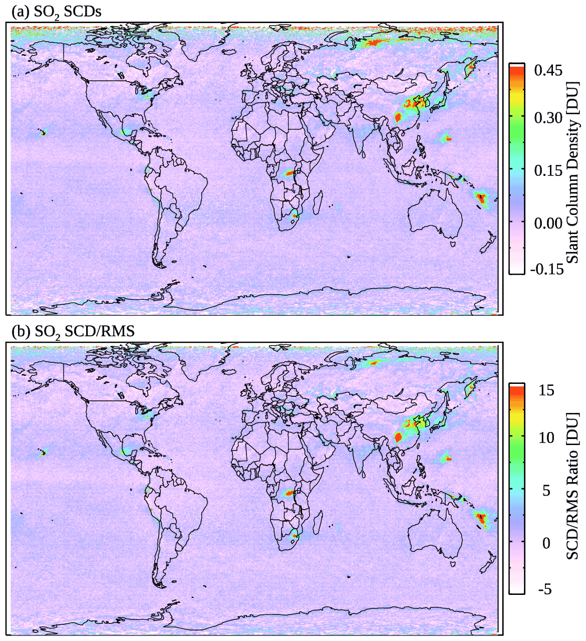
Figure 2(a) Monthly mean OMI SO2 SCDs for March 2005 showing enhanced SO2 signals over major anthropogenic source areas (e.g., China, the eastern US, India, and South America) as well as degassing volcanoes. Note the positive bias at northern high latitudes. (b) Monthly mean SCD rms ratio (SRR) from the same sample of OMI pixels as in panel (a). The SRR map also shows major SO2 sources but has reduced bias at high latitudes compared with the SCD map.
2.2 Classification of OMI pixels
The purpose of the pixel classification scheme (Fig. 1b) is to compile a training dataset by selecting pixels in two categories: (1) the first for clean pixels in which the retrieved SCDs are relatively small while the fitting errors are relatively large (i.e., negative or small positive SRRs) so that they can be considered largely SO2-free and (2) the second in which the retrieved SCDs are large while the fitting errors are relatively small (i.e., large SRRs). In this category for polluted pixels, the retrieved SCDs are assumed to be close to the truth. There are two additional categories. The third is for pixels that fall between the clean and polluted categories. For these pixels, an unambiguous classification cannot be made and they are excluded from the training dataset. The fourth category (high SRR) is for pixels that have very large SRRs (>300). Such pixels are few but are also excluded from the training, as they tend to have a disproportionally large influence on the trained NNs.
In addition to the SRRs of individual OMI pixels, the classification scheme also takes into account the location (latitude–longitude) of the pixels, as well as the general performance of the PCA algorithm for the latitude bands in which they are located. A pixel with a specific SCD rms ratio of SRRi is considered to be polluted if
The pixel would be considered to be clean if
where and σSRR are the monthly medians of the daily mean and standard deviation of SRRs for the corresponding latitude band, respectively. a1 and a2 are scaling factors (see Fig. 1b for values) that have been adjusted through trial and error in order to (1) minimize the artifacts in NN-analyzed SCDs over background areas and (2) maximize the retained original SO2 signals over polluted areas. Both factors depend on the location of the pixels and the monthly mean SRRs (SRRm). As shown in Fig. 1b, a1 and a2 are large if the pixel is located in an area with a small SRRm (<3). In this case, the area is generally unpolluted and the likelihood of a pixel containing a positive SO2 value is low. Thus, more pixels are classified as clean. On the other hand, for polluted areas with large SRRm (>5), both a1 and a2 are kept small so that more pixels would be classified as polluted. For areas that are moderately polluted (i.e., ), a1 and a2 are linearly interpolated based on the SRRm. One may also notice that a1 and a2 are smaller for low (30∘ S–30∘ N) and middle (30–60∘ S and 30–60∘ N) latitudes than for high latitudes. This helps to reduce the positive bias in the original SCDs near the northern edge of the domain (Fig. 2a). We also tested a simple classification scheme with constant a1 and a2 everywhere, and we found that it produces relatively large positive biases over high latitudes and negative biases over low-latitude source areas compared with the more complicated scheme described above. It should also be pointed out that the areas affected by the South Atlantic anomaly (SAA) are not subject to classification and are excluded from the training dataset.
Using the classification scheme, one can also develop a simple method to reduce retrieval artifacts by assuming that clean pixels should have zero SCDs, while polluted pixels should retain their original SCDs, and by estimating SCDs for pixels that fall in between through a linear interpolation (between zero and the original SCDs). As will be demonstrated in Sect. 4.4, such an approach produces negative biases over polluted areas. It is thus advantageous to employ the more complex NN-based method for the present study.
2.3 Training of neural networks
For training data, we use the OMI pixels identified as either clean or polluted by the classification scheme. For a typical day, approximately ∼800 000 out of ∼1 million OMI pixels are classified as clean and ∼10 000 (∼1 %) as polluted. Given the scarcity of ground-truth SO2 data, we set the training target (SCDtarget) to zero for the clean pixels and to the original SCDs for the polluted pixels. Note that unlike the PCA spectral fitting algorithm, data from all 60 rows are pooled together in the training so that a relatively large sample of polluted pixels is available. We also include several candidate predicators in the training data, including SCD rms ratios for the individual pixels (SRRi), the monthly mean SCD rms ratios (SRRm) where the pixels are located, the cosines of solar zenith angles (SZA, θ0), viewing zenith angles (θ), and phase angles (ϕ), the O3 column amounts from the OMI total O3 product (OMTO3, Bhartia, 2005), and the scene reflectivity (R) at 354 nm from the OMI Raman cloud product (OMCLDRR, Joiner and Vasilkov, 2006). The function of a neural network (NN) is then to use the input predictors or features to predict the output SCDtarget:
To optimize the set of predictors, we carried out a number of tests using different combinations (see Table 1 for example results). Among the predictors, SRRi is well correlated with SCDtarget and has the largest impact on the performance of the NNs. Indeed, the NN without SRRi produces the lowest correlation coefficient (r) and the largest root mean square error (RMSE) between the analyzed SCDs (SCDNN) and SCDtarget (Table 1). SRRm provides geospatial context for the NNs so that higher SCDs tend to be assigned to polluted areas. In the particular example in Table 1, a simple NN using just SRRi and SRRm as predictors produces SCDNN that agrees reasonably well with SCDtarget (r=0.958, RMSE =0.0517 DU). The angles, O3 column amounts, and scene reflectivity all affect the signal-to-noise ratio of OMI measurements and the quality of SO2 retrievals (Li et al., 2020). Adding them as predictors generally leads to small but noticeable improvements in the performance of the NNs (Table 1). While the NN with all seven predictors has slightly worse performance than the NN without SRRm for this case, including SRRm as a predictor helps to retain signals over SO2 source areas. We also tested additional predictors (e.g., the terrain pressure and the scene pressure) and found no discernible improvements in the overall performance of the NNs. Hereafter we use all seven predictors as specified in Eq. (3) in the NNs.
Table 1The correlation coefficient (r) and root mean square error (RMSE) between the NN-analyzed OMI SO2 SCDs (SCDNN) using different predictors and the target SCDs (SCDtarget). The NNs are trained using data from 5, 10, 15, 20, and 25 July 2005. The comparisons shown here are for pixels from the same days but not included in the training.

* Results shown are from a simple linear regression analysis.
The architecture of the NNs in this study (Fig. 1c) is similar to that employed by Joiner et al. (2021, 2022) for reconstruction of RGB images from hyperspectral radiances. A similar architecture has also been used to capture changes in gross primary production (GPP) from satellite reflectance data (Joiner and Yoshida, 2020). Briefly, the artificial feed-forward NNs are implemented in IDL (Interactive Data Language) and contain two hidden layers, each with 14 nodes (twice the number of predictors), and an output layer with one node. Experiments using more (up to 30) nodes in each hidden layer yield little difference in the performance of the NNs. The activation functions are a soft sign for the first hidden layer, a logistic (sigmoid) for the second hidden layer, and a bent identity for the output layer. If we replace the activation functions in both hidden layers with ReLU (Rectified Linear Unit), the NNs converge faster in training but increase the SCDs over background areas by ∼ 0.01–0.02 DU (Fig. S1 in the Supplement). An adaptive moment estimation (Adam) optimizer (Kingma and Ba, 2014) with a learning rate of 0.1 is used to minimize the error. Inputs and outputs are normalized so that they each have a mean of zero and a unit standard deviation.
For each month, we train a neural network (NN1, Fig. 1) utilizing data from 5 d (the 5th, 10th, 15th, 20th, and 25th days of the month). Half of the clean and polluted pixels are used in the training and the rest for evaluation. We notice that NN1 reproduces SCDtarget well for clean pixels and also for polluted pixels that have SCDs up to ∼ 4–5 DU, but it produces a low bias for larger SCDs. This is likely due to the imbalance between the clean and polluted categories in the training data. To mitigate this issue, we use the pre-trained NN1 only for clean and in-between pixels (Fig. 1a) and a separate neural network (NN2) for polluted pixels from each day (Fig. 1a). NN2 has the same architecture as NN1 but is trained daily with half of the polluted pixels. Alternatively, we can also train NN2 using data from multiple days and apply the pre-trained multi-day model to the entire month. Compared with the daily trained NN2, SCDNN produced by the multi-day model is similar but slightly lower over some polluted areas (e.g., eastern China). To maximize the retained SO2 signals over those regions, we use daily trained NN2 in the present study.
In the final step (Fig. 1a), the SCDNN outputs from NN1 and NN2 are merged with the original SCDs for high-SRR pixels to produce the final NN-analyzed SCDs.
3.1 Daily comparisons of SO2 SCDs
In Fig. 3, we compare the NN-analyzed SO2 SCDs (SCDNN) and the target SCDs (SCDtarget) from 16 January, April, July, and October 2005 for independent pixels that are not part of the training. There is generally good agreement between SCDNN and SCDtarget, with r>0.93 and RMSE at ∼ 0.02–0.03 DU for all 4 d. The vast majority of clean pixels as identified by the classification scheme have SCDNN between −0.1 and 0.1 DU, indicating substantial reduction in the retrieval noise compared with the original retrievals (1σ noise of ∼ 0.2–0.3 DU), although a small fraction of the clean pixels still have SCDNN as large as ±0.5 DU. The slopes from the linear regression analysis are between 0.95 and 0.98, suggesting slight underestimates in SCDNN. There is also some scatter for the polluted pixels, particularly at higher SCDs (>2 DU). The number of pixels having large SCDtarget is relatively small, and this limit in the training data may affect the performance of NNs under high-SCD conditions (such as for volcanic plumes). We repeated the analysis for the whole year and found similar results for most days. On average, the correlation coefficient from the daily comparisons is 0.948±0.0309 (hereafter results are shown as mean ± standard deviation) and the RMSE is 0.0343±0.0194 DU, while the slope is 0.966±0.0409. There are 4 d with RMSE >0.1 DU (6 April, 11 June, 13 July, and 14 August). All four have relatively large errors over areas affected by volcanic plumes, again suggesting that the NN performance may deteriorate at high SCDs. Overall, the comparisons here point to quite good performance of the NNs in reproducing the target SCDs.
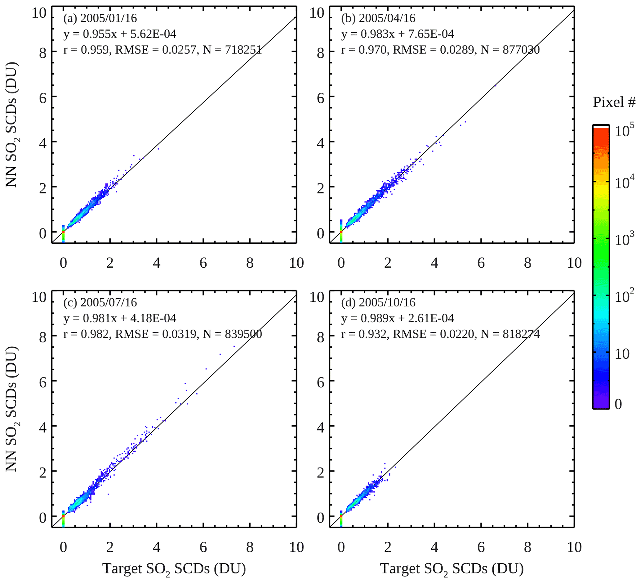
Figure 3Scatter plots between the NN-analyzed SO2 SCDs and the target SO2 SCDs for clean and polluted OMI pixels from the 16th day of (a) March, (b) April, (c) July, and (d) October 2005. Only pixels not used in the training of the neural networks are shown. Colors represent the number of data points within each 0.1 DU (in NN SCDs) by 0.1 DU (in target SCDs) bin. The solid line in each panel represents the best fit through the data from the simple linear regression analysis between NN and target SCDs. The slope and intercept from the regression are given in each panel, along with the correlation coefficient (r), root mean square error (RMSE), and number of pixels (N).
Compared with the original SCDs, the NN-analyzed SCDs have highly reduced noise and artifacts over background areas and largely retain SO2 signals over polluted regions. This is evident from Fig. 4, which shows the original SO2 SCDs, the NN-analyzed SCDs, their differences, and the mean SCDs for different latitude bands over generally clean areas (monthly mean SRR <3) for 16 April 2005 as an example. As can be seen from the figure, the NN-analyzed SCDs show little variation with latitude compared with the original PCA retrievals (Fig. 4d). The differences between the two (Fig. 4c) are similar to the original SCDs (Fig. 4a) over most background areas, as ∼80 % of the pixels are identified as clean and have SCDNN within ±0.1 DU. The differences are quite small over polluted regions (e.g., eastern China, Sichuan Basin, Norilsk), as pixels over those areas tend to be classified as polluted and have SCDNN close to their original retrievals. It is worth mentioning that even though the SAA-affected areas are excluded from training, the analyzed SCDs over those areas still show smaller noise than the original ones. One potential reason is that retrievals over the SAA areas tend to have relatively large rms, and the use of SRRs partially cancels out the relatively noisy SCDs.
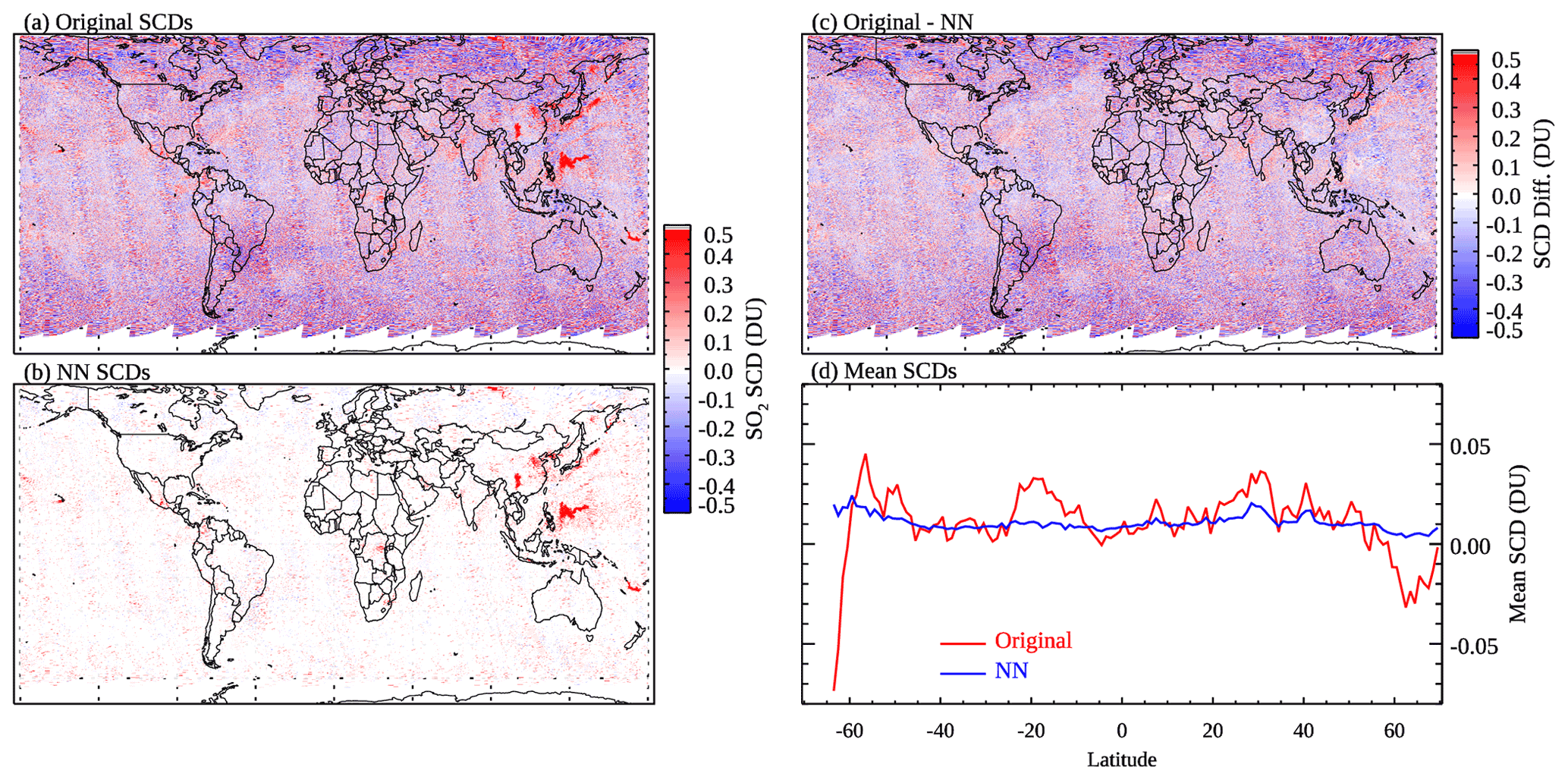
Figure 4The (a) original, (b) NN-analyzed OMI SO2 SCDs and (c) their differences for 16 April 2005. (d) Mean SO2 SCDs for 1∘ latitude bands over generally clean areas (monthly mean SRR <3), calculated from (red) the original and (blue) NN-analyzed SCDs for the same day.
3.2 Comparisons of monthly SO2 SCDs
The monthly maps in Fig. 5 for March 2005 show consistent results with the daily comparisons in Sect. 3.1. While the monthly mean SCDs from the original PCA retrievals (Fig. 5a) are close to zero for most background areas, biases are evident over certain regions. For example, there are patches of negative SCDs (approximately −0.1 DU) at ∼ 40–60∘ N and over the oceans near the Equator. Another noticeable feature is the negative bias over the relatively bright arid and semi-arid land surfaces such as the Sahara, the Arabian peninsula, and the Taklimakan and Gobi deserts. It is possible that the retained PCs (derived from hundreds of pixels from each OMI row) do not fully capture certain interfering factors for those areas. The exact reasons for these artifacts are unknown and beyond the scope of the present study. In any case, they are largely removed through our NN-based analysis (Fig. 5b). Meanwhile, there is no obvious difference between the original and analyzed SCDs over major SO2 source areas (Fig. 5c), which is evidence that the NNs have learned to preserve the SO2 signals over those areas.
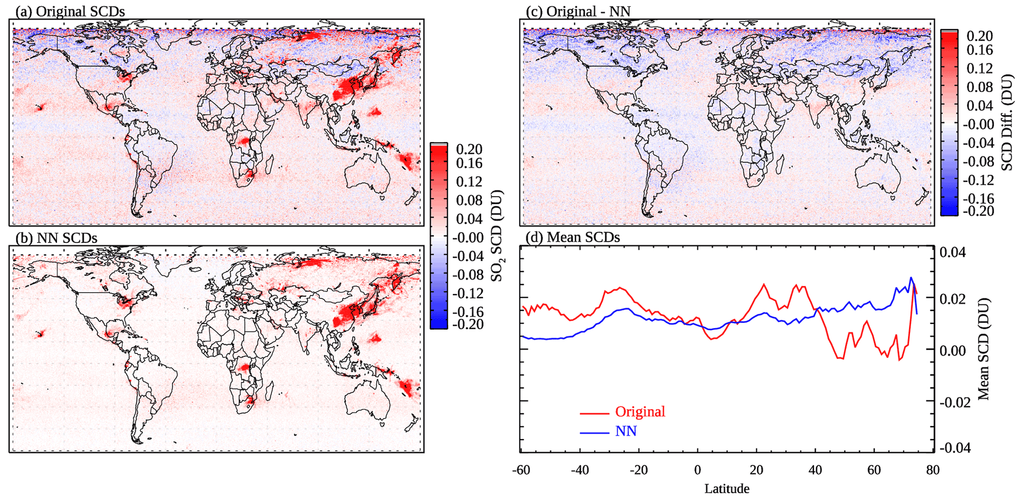
Figure 5Similar to Fig. 4 but showing monthly means for March 2005.
One may notice that outside the source regions, the difference map in Fig. 5c is not identical to the original SCD map in Fig. 5a. For example, the differences are slightly more negative than the original SCDs over parts of Canada, Mongolia, and Russia. Most pixels have SCDNN near zero, but some pixels with noisy, positive original SCDs could be misclassified as polluted, resulting in a small positive bias in SCDNN for these areas. This is also noticeable in Fig. 5d that shows the mean original and NN-analyzed SCDs within 1∘ latitude bands over clean areas. The NN SCDs have generally less structure, indicating reduced artifacts, but a positive bias of ∼0.02 DU can be found north of 60∘ N. Mean SCD maps for other months (January, April, July, October 2005; see Fig. S2) show quite similar results. For areas and/or periods strongly influenced by relatively large volcanic eruptions (e.g., the Sierra Negra, Galapagos Islands, eruption in October 2005), the NNs have difficulty completely reproducing the strong SO2 signals. This again points to the slightly deteriorated performance of NNs under high-SO2 conditions, as already discussed.
A close-up look at the NN-analyzed SCDs and their differences from the original SCDs over eastern China is given in Fig. 6. For polluted areas (analyzed SCDs >0.15 DU), the relative differences are typically within ±20 %, with a mean of 4 % (with the original SCDs being greater). For background areas, the relative differences are close to ±100 % as expected for clean pixels. Comparisons for other major anthropogenic source areas including India, the Middle East, South Africa, the eastern US, and Norilsk (Russia) yield similar results (see Figs. S3–S7). The mean relative differences for polluted areas in these regions are all within ±15 %, ranging between −11 % for the eastern US and 14 % for the Middle East. In comparison, the relative differences for areas affected by large volcanic plumes are greater, for example reaching 20 % on average over part of the southeastern Pacific during the October 2005 Sierra Negra eruption (see Fig. S8).
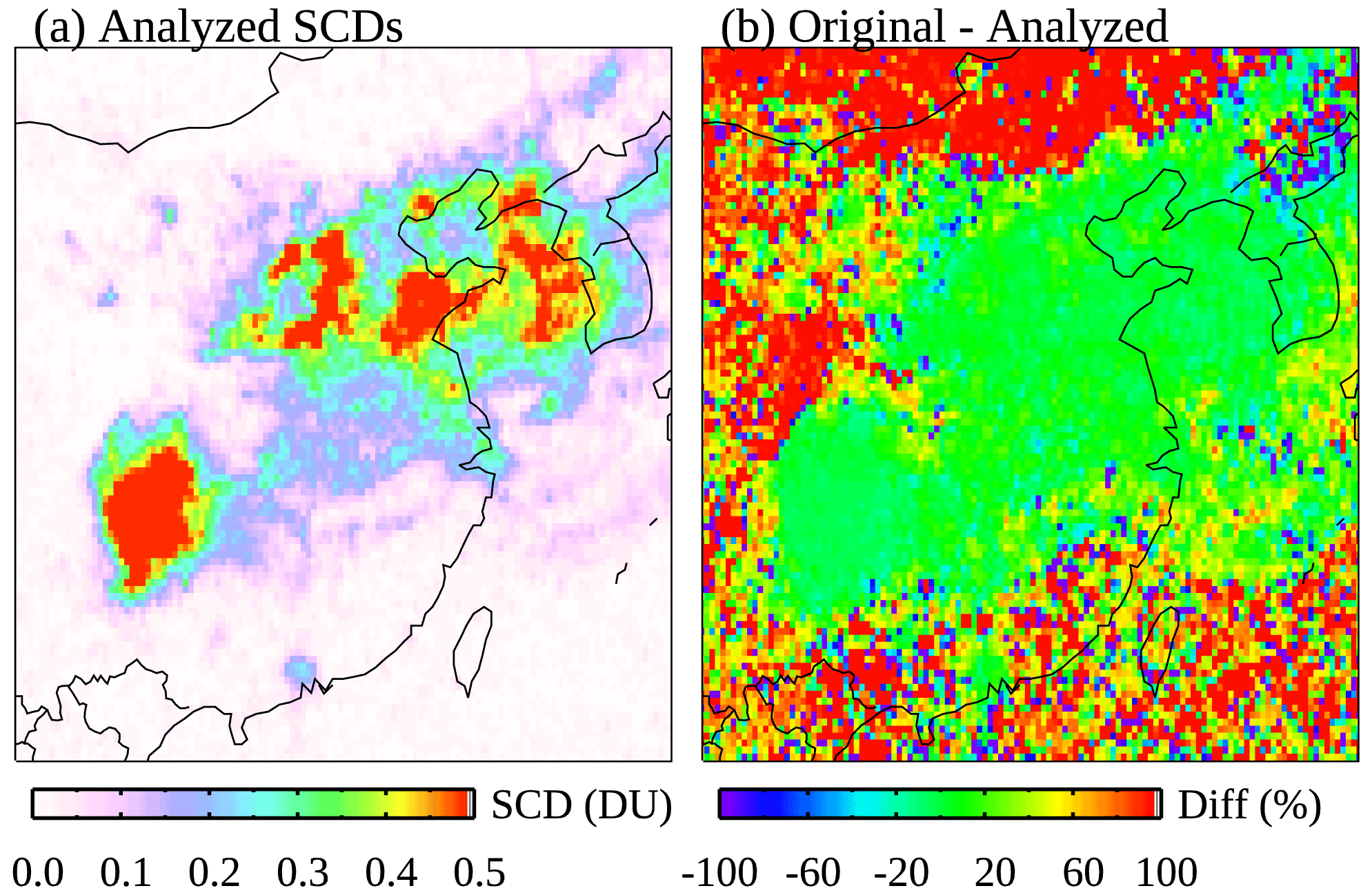
Figure 6(a) The NN-analyzed SO2 SCDs and (b) their relative differences from the original SCDs over eastern China for March 2005.
4.1 Original and analyzed SO2 SCDs as a function of SRRs
The results presented in Sect. 3 demonstrate that our NN-based analysis can reduce noise and artifacts for clean pixels while largely retaining the original SCDs for polluted pixels. However, some key questions remain unanswered. Namely, given the somewhat subjective criteria used in the pixel classification scheme (Sect. 2.2) to build the training data, do we risk removing real SO2 signals as noise (i.e., overcorrection) and/or keeping noise and artifacts as signals (i.e., under-correction)? Another related question is how do the NNs treat pixels that are not in the training data (i.e., the pixels that fall between the clean and polluted categories)? To shed light on these issues, we calculate the monthly mean SO2 SCDs as a function of pixel-level SCD rms ratios (SRRi) from the original retrievals (panel a of Figs. S9–S13) and the analyzed data (panel b of Figs. S9–S13), as well as their differences (Fig. 7, left) for March 2005. In addition, we also calculate the mean original and NN-analyzed SCDs as a function of latitude for different ranges of SRRi (Fig. 7, right).
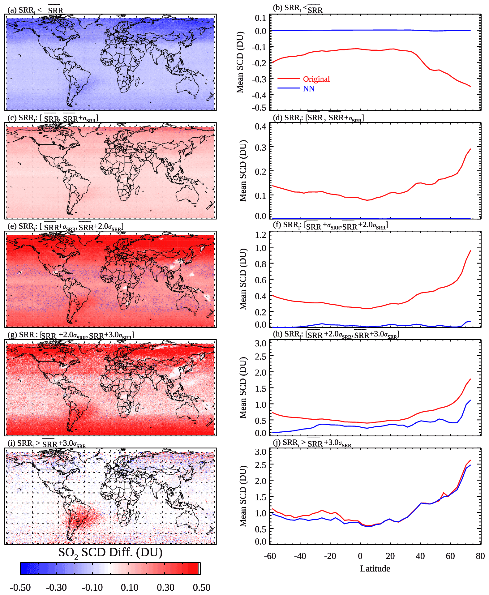
Figure 7(a, c, e, g, i) The differences between the original and NN-analyzed OMI SO2 SCDs for March 2005. (b, d, f, h, j) The mean (red) original and (blue) NN-analyzed SCDs for 3∘ latitude bands for the same month. Different rows show results from pixels that have SCD rms ratios (SRRi) within different ranges based on the monthly medians of the daily mean () and standard deviation (σSRR) of SRRs for their corresponding latitude bands: (a–b) , (c–d) , (e–f) , (g–h) , and (i–j) .
For pixels having (see Sect. 2.1 for definitions of and σSRR), the original SCD map (Fig. S9a) shows no obvious hotspots even over the major SO2 source areas. All such pixels would be classified as clean, and indeed the mean NN-analyzed SCDs (Fig. S9b) from these pixels are zero everywhere. The mean analyzed SCDs (Fig. 7b) are also near zero at all latitudes.
The next group of pixels have (Fig. 7, second row). Most pixels in this group, except for those near large SO2 sources at low latitudes (30∘ S–30∘ N), would also be classified as clean. Similar to the first group, there are no obvious SO2 hotspots in the original SCD map (Fig. S10a). The analyzed SCDs (Fig. S10b) are similarly near zero almost everywhere, with notable exceptions over some degassing volcanoes (Anatahan, Nyiragongo, and Vanuatu) and heavily polluted areas (Sichuan Basin and Norilsk). The case of Norilsk is particularly interesting. Given the thresholds for high latitudes (Fig. 1b), all pixels in this group over Norilsk would be classified as clean, but the NNs seem to be able to override the classification based on factors other than SRRs. The mean analyzed SCDs are around zero for all latitude bands, which is smaller than the original SCDs (Fig. 7d).
For the group of pixels having intermediate SRRs (, Fig. 7, third row), the original SCD map (Fig. S11a) contains enhanced SO2 signals over source areas but also artifacts over background regions. The pixels in this group would be classified as clean, polluted, or in between depending on their SRRi and locations. In general, the NNs are able to largely eliminate the artifacts and retain signals over SO2 source areas for this group (Fig. 7e), although there are remaining small positive biases both near the northern edge of the domain and at lower latitudes (e.g., around 30∘ S) as shown in Fig. 7f.
For the following group (, Fig. 7, fourth row), almost all pixels would have a classification of either polluted or in between. NNs reduce the retrieval artifacts in this group, particularly at middle to high latitudes (Fig. 7g and h). The relatively small changes at low latitudes can probably be attributed to the more relaxed thresholds for pixels to be classified as polluted and in between (Sect. 2.2). Using more stringent thresholds may further reduce the artifacts in the tropics, but this may also lead to low bias over pollution sources (see Fig. 8b for example).

Figure 8(a) Differences in the analyzed OMI SO2 SCDs for March 2005 between NNs trained using pixels classified with a1 and a2 (see Eqs. 1 and 2) scaled to 90 % of the baseline values in the classification scheme and those trained with the baseline scheme. (b) Same as (a) but for a1 and a2 scaled to 110 % of the baseline values. (c) Mean SCDs for 1∘ latitude bands over relatively clean areas (monthly mean SRR<3) using NNs trained with pixels from different classification schemes: (black) the baseline a1 and a2, (blue) a1 and a2 scaled to 90 %, and (red) a1 and a2 scaled to 110 % of the baseline values.
For the final group (, Fig. 7, fifth row), almost all pixels are identified as polluted. As a result, the differences between the original and analyzed SCDs are quite small except over the SAA-affected areas (Fig. 7i and j at around 30∘ S) where the pixels are not part of the training data and the noise is reduced by the NNs. Overall, it is encouraging that the NN-analyzed SCDs show improvements over the original ones for all ranges of SRRs.
4.2 Sensitivity of NN-analyzed SCDs to the pixel classification scheme
We further test the sensitivity of NN-analyzed SCDs to the settings of the pixel classification scheme by altering the a1 and a2 parameters (Eqs. 1 and 2). In one experiment, we scale both parameters by 90 % (i.e., reduced by 10 % from the baseline values as specified in Fig. 1b). This leads to more pixels being classified as polluted and greater monthly mean SCDs (Fig. 8a). The increase in the SCDs is ∼ 0.01–0.02 DU on average over relatively clean areas (Fig. 8c) and slightly larger over some source areas (e.g., eastern China) but typically less than 0.1 DU. In another experiment, both a1 and a2 are scaled by 110 % (i.e., increased by 10 % from the baseline values), resulting in SCD reductions of ∼0.01 DU over clean areas (Fig. 8c). Some source areas (e.g., Norilsk) show slightly more reductions (Fig. 8b) that are still typically less than 0.1 DU. Overall, the tests here point to moderate sensitivity of the NN-based analysis to the settings of the pixel classification scheme. An overly stringent scheme may lead to overcorrection and low biases over source areas, whereas an overly relaxed scheme may result in positive biases. For our particular study, any overcorrection or under-correction appears to be minor for major source areas, given the relatively small differences between the analyzed and original SCDs (see Sect. 3.2). But if one is to apply the technique to other datasets (e.g., different instruments and/or species), the pixel classification scheme will need to be tested and optimized. For long-term analysis of a dataset from a single instrument (e.g., OMI SO2 for the entire mission), the scheme will need to be verified using data from different years, although we envision that a constant set of a1 and a2 parameters over time will probably be more suitable to avoid artificial trends introduced by time-dependent parameters. For future studies, we plan to develop a more systematic way to classify pixels, for example by using more objective metrics.
4.3 SO2 emission estimates using the original and NN-analyzed SCDs
Another test involves running both the original and NN-analyzed SCDs through a top-down emission estimation algorithm to derive annual SO2 emissions from large point sources. Here we focus on anthropogenic sources, given the low bias in the NN-analyzed SCDs for large volcanic plumes. We infer SO2 emissions by fitting oversampled and smoothed OMI vertical column densities (VCDs) to a three-parameter (i.e., total mass, lifetime, and plume spread) function of horizontal coordinates and wind speeds (Fioletov et al., 2015). To convert SCDs to VCDs, we use the same air mass factors (AMFs, VCD = SCD AMF) as in Fioletov et al. (2016). For wind fields, we use the average winds between the surface and ∼1 km from GEOS-5 Forward Processing for Instrument Teams (FP-IT) assimilated products that have been co-located with OMI (OMUFPITMET; available at https://disc.gsfc.nasa.gov/datasets/OMUFPITMET_003/summary, last access: 17 September 2022). The OMI pixels are then rotated around known source locations according to wind directions such that all observations are aligned in the upwind–downwind direction (Fioletov et al., 2015). Following Fioletov et al. (2016), we prescribe the SO2 lifetime (6 h) and the parameter describing the spread of the emitted plume (20 km) to obtain more robust fitting results. Only one parameter, the total SO2 mass, is estimated from the fit. We further derive SO2 emissions by dividing the fitted total SO2 mass by the prescribed lifetime. For fitting uncertainty, we calculate the 1 standard deviation error in the fitted parameter by taking the square root of the diagonal elements of the covariance matrix of the parameter.
As shown in Fig. 9a, the two sets of emission estimates agree quite well (r>0.99, slope >0.96), suggesting the NN analysis has largely preserved SO2 signals in the original retrievals. In general, the estimated emissions using the NN-analyzed SCDs are slightly smaller than those based on the original retrievals, particularly for relatively small sources (<20 kt, 103 t yr−1). While on the surface this may suggest loss of some real SO2 signals in our analysis for relatively small sources, the emission uncertainties (Fig. 9b) for those sources also become much smaller when using the NN-analyzed data. This leads to greater emission-to-uncertainty ratios (Fig. 9c) for those sources, implying that the reduced noise and artifacts in the analyzed data may facilitate SO2 source detection and quantification. We note that the results here should be interpreted with caution, given that OMI sensitivity to sources <30 kt yr−1 is quite limited (Fioletov et al., 2015).
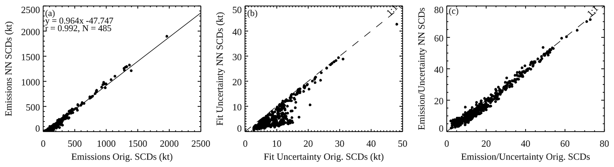
Figure 9Scatter plots comparing (a) the annual emission estimates for 485 large point sources for 2005, (b) the uncertainties in the emission estimates, and (c) the ratios between the emission estimates and the uncertainties using the NN-analyzed vs. the original SCDs. All sources shown here are anthropogenic and have emission estimates at least twice the uncertainties for both datasets.
4.4 Can a simple linear interpolation model reproduce NN-analyzed SCDs?
Given the seemingly simple assumptions made about the clean and polluted pixels during the training process (Sect. 2.3), one may also ask whether there is any advantage to using the NN-based data analysis approach. To test this, we apply the same pixel classification scheme as described in Sect. 2.2 and build a simple model by assigning zero SCDs to the clean pixels, assigning the original SCDs to the polluted pixels, and linearly interpolating between zero and the original SCDs for pixels that fall in between (based on the SRRs for those pixels and the corresponding thresholds as defined in Eqs. 1 and 2).
The mean SCDs for March 2005 (Fig. 10a), produced with this simple linear interpolation model, appear to be quite similar to those produced with the NN-based analysis (Fig. 5b). This is not surprising since the majority of pixels are classified as clean, and NN-analyzed SCDs for those pixels are also close to zero. The plot of mean SCDs as a function of latitude (Fig. 10c) also indicates overall comparable results for relatively clean areas between the two methods, although the linear model has more obvious step changes at 30∘ N and 30∘ S probably related to the pixel classification scheme. Over pollution source areas (e.g., eastern China), on the other hand, the linear model has a substantial negative bias compared with the NN-based approach (see the SCD difference map in Fig. 10b). Additionally, the noise is also larger over the SAA areas for the linear model. This comparison demonstrates some advantages in the NN-based approach, particularly for preserving SO2 signals over source areas. It should be mentioned that the simple linear model tested here can be potentially improved by including more predictors such as those used in the NNs (e.g., monthly SRRs, the Sun–satellite geometry, and O3). But such a multi-regression model may need to be optimized locally for different regions and can be more challenging to implement compared with the NNs.
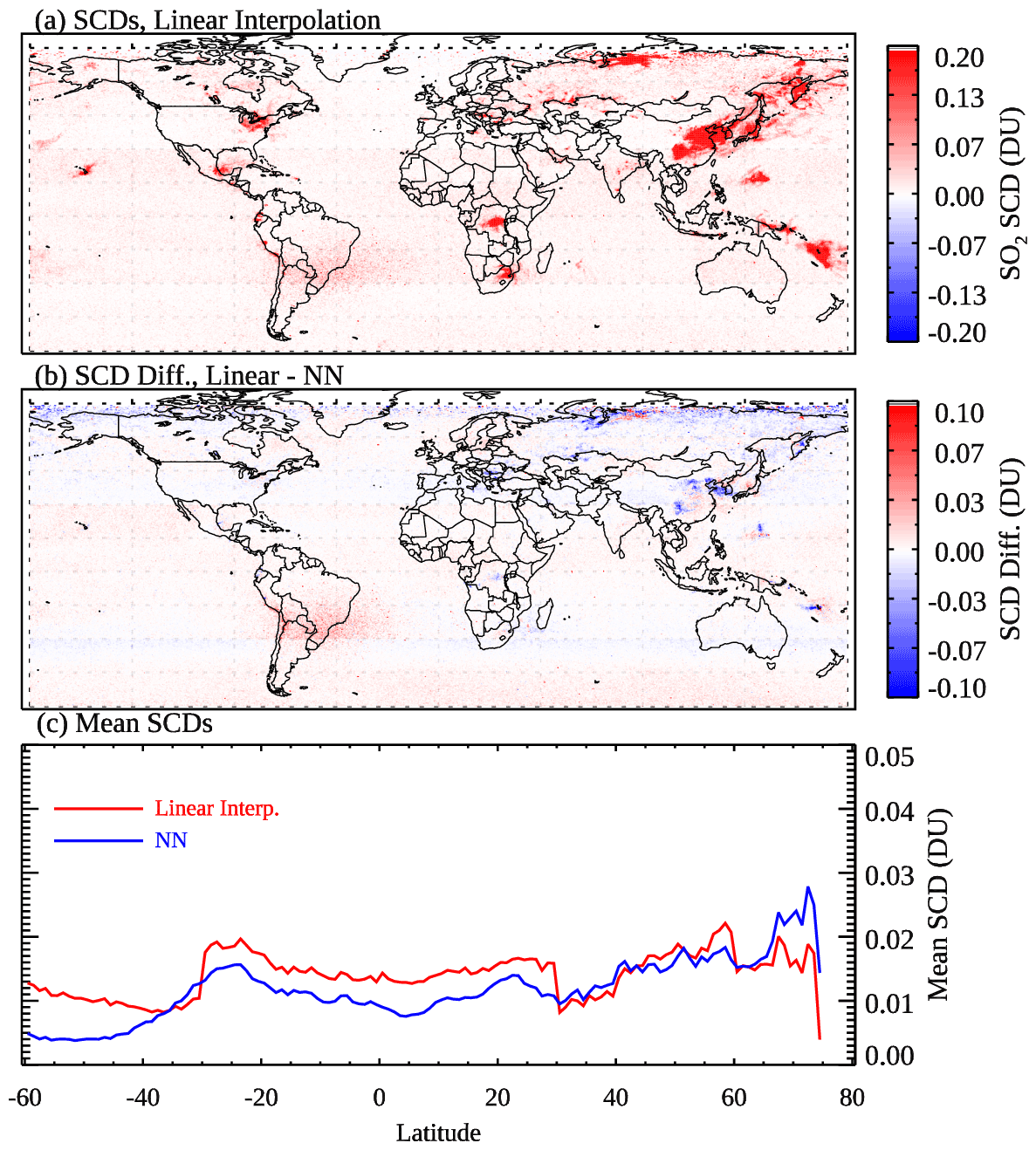
Figure 10(a) Monthly mean OMI SO2 SCDs for March 2005, analyzed using a simple linear interpolation model. (b) The differences in the analyzed SCDs between the linear model and the neural networks. (c) Mean SCDs for 1∘ latitude bands over generally clean areas (monthly mean SRR<3), calculated from the SCDs from (red) the linear interpolation model and (blue) the NNs.
4.5 Implementation of a PCA–NN SO2 fitting algorithm
So far, we have relied on the output from the existing PCA SO2 algorithm as input to the NNs; therefore, our method can be viewed as an additional data processing step following the spectral fit. For a potential alternative to this approach, we also attempt to build an NN-based SO2 SCD fitting algorithm that uses the measured radiances as inputs and the NN-analyzed SCDs for training targets. As with the PCA SO2 algorithm, the NN fitting algorithm uses the logarithm of Sun-normalized Earthshine radiances at 310.5–340 nm and processes each OMI row separately with individually trained NNs. We pool the data from 12 d in 2005 (the 10th day of each month), generating a training dataset that contains about 200 000 pixels for each row. To reduce the data dimension of the inputs, a PCA technique is combined with the NNs in this PCA–NN fitting algorithm as in Joiner et al. (2022). We conduct PCA on the radiance spectra and include the coefficients of the first 50 leading PCs as predictors in the NNs. Experiments using fewer (as few as 20) or more (up to 100) PCs generally result in larger errors in the retrieved SCDs. In addition to the PC coefficients, the NNs also use four other parameters (solar zenith angles, O3 column amounts, scene reflectivity, and monthly mean SRR ratios) as predictors. Viewing zenith angles are not included since the training is carried out separately for each row. We also exclude the phase angles, given that adding them as a predictor leads to no discernible improvements in the algorithm performance. The SRRs for individual pixels are also excluded, as the PCA–NN algorithm is designed to run independently from the PCA SO2 algorithm after the training phase. While the monthly mean SRRs also originate from the PCA retrievals, they essentially provide geospatial context on the spatial distribution of SO2 and can be potentially replaced with other datasets such as SO2 emission inventories or model-simulated SO2.
For the PCA–NN algorithm, we utilize an NN architecture similar to that in Fig. 1c, with the only difference being that the number of nodes in each hidden layer is now 108 (twice the number of the predictors). For each row, we train an NN using half of the pixels and the rest for evaluation. The pre-trained NNs are then applied to SO2 SCD retrievals for 16 April 2005, a day not used in the training.
The results shown in Fig. 11 indicate that the PCA–NN algorithm can reduce the retrieval noise over background areas compared with the original PCA SO2 algorithm. However, over polluted areas and degassing volcanoes, the PCA–NN retrieved SO2 is biased low (Fig. 11c). This suggests that the PCA–NN algorithm, with its present implementation, cannot yet achieve the same level of performance as our NN-based data analysis on the original PCA retrievals. It is possible that due to the much smaller number of polluted pixels compared with the clean ones, some spectral signatures of SO2 are lost in the first 50 or even 100 PCs, leading to the low bias over polluted areas. The NNs may need to include more PCs as predictors or directly use radiances without the transformation. A separate set of NNs trained on a refined dataset that contains more polluted pixels may also help to mitigate the bias. But applying these NNs to retrievals would require some prior knowledge about the status of the pixels (whether they are polluted or clean). Also, the PCA–NN retrievals show some striping features, probably reflecting the different performance of the NNs for different rows despite the use of the same architecture. The reason for this row-to-row change in performance is not yet understood. Nonetheless, the PCA–NN algorithm shows promise and will be the subject of more in-depth studies in the future. For example, the training performance may improve if the architecture is optimized for each row.
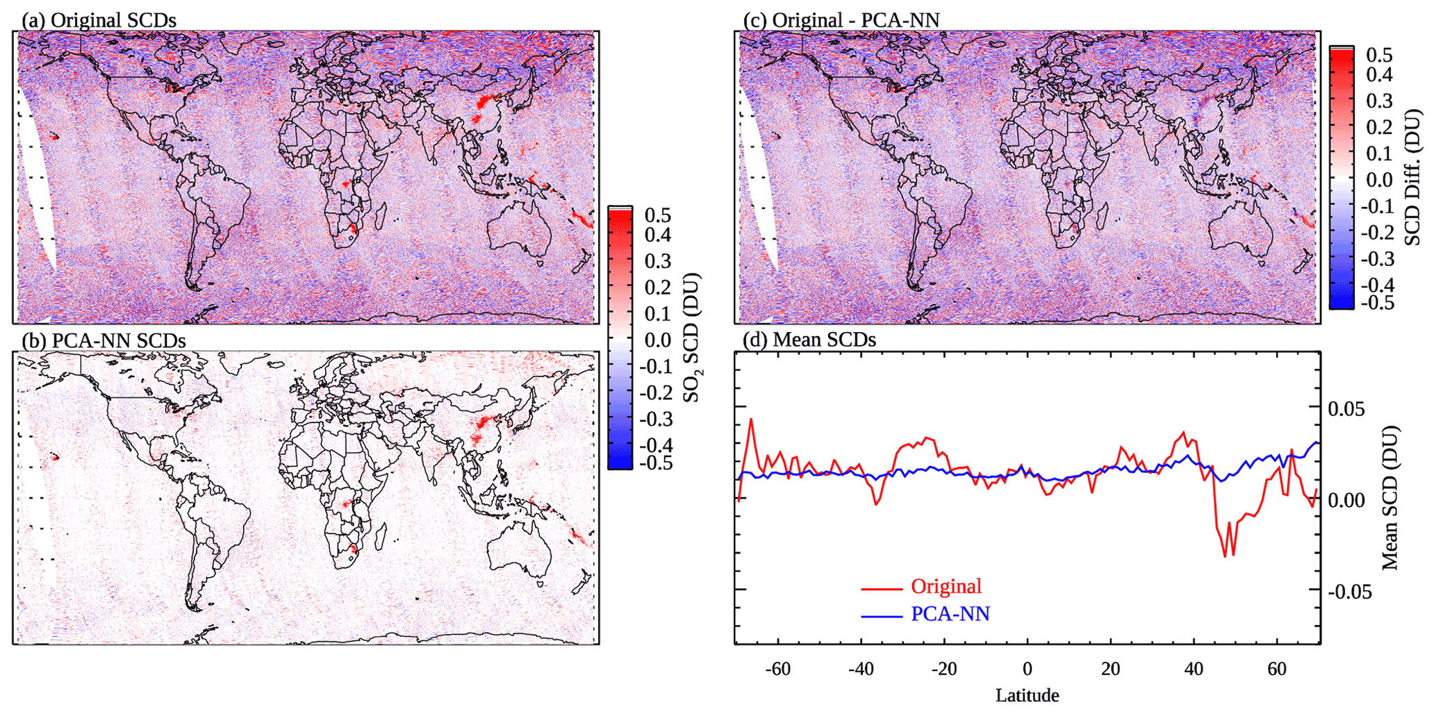
Figure 11OMI SO2 SCDs for 16 April 2005 retrieved using (a) the original PCA algorithm and (b) a PCA–NN algorithm, (c) the differences between the two retrievals, and (d) mean SO2 SCDs for 1∘ latitude bands over relatively clean areas (monthly mean SRR<3), calculated from (red) the original and (blue) PCA–NN retrievals.
We have developed a new machine-learning-based method to analyze satellite-retrieved atmospheric composition data, with the aim of reducing the noise and artifacts while retaining the signals in the original retrievals. To demonstrate this approach, we use OMI SO2 SCDs retrieved with the PCA-based spectral fitting algorithm as an example. A key parameter in the analysis method is the SRR, which is the ratio between the retrieved SCD and the rms of the fitting residuals. Based on prior knowledge about the global distribution of SO2 pollution (from existing in situ measurements and model simulations), we assume that a given pixel with a small (large) SRR is likely clean (polluted) and its real SCD should be close to zero (the original retrieved SCD). This allows us to overcome the lack of ground-truth data and build a training dataset for SO2 by selecting clean and polluted pixels from the original retrievals.
We then train neural networks (NNs) using the compiled dataset. The NNs contain two hidden layers with 14 nodes each and one node in the output layer for the analyzed SCDs. The predictors for the NNs include SRRs for individual pixels, solar zenith, viewing zenith and phase angles, scene reflectivity, and O3 column amounts, as well as the monthly mean SRRs. The latter provide context for the spatial distribution of SO2, whereas the other predictors (angles, O3, and reflectivity) affect the quality of the original SCDs. The function of the NNs is to connect these predictors to the target SCDs (zero for clean pixels, the original SCDs for polluted pixels in the training data). For data analysis, we employ a hybrid model (Fig. 1) that includes two NNs: (1) an NN pre-trained using 5 d of data from each month to produce analyzed SO2 SCDs for pixels that are clean or moderately polluted (i.e., those with SRRs between clean and polluted pixels) for the entire month and (2) an NN trained daily to produce analyzed SCDs for the polluted pixels each day. This hybrid model helps to maximize the retained SO2 signals over source areas.
Results for 2005 show that the NNs can reproduce the target SCDs well and largely reduce noise and artifacts in the original retrievals. For polluted areas, the monthly mean SCDs from the analysis are mostly within ±15 % from the original retrievals, indicating that the NNs are able to preserve SO2 signals. This is confirmed by another experiment in which the NN-analyzed and original SCDs are used to estimate the SO2 emissions for ∼500 anthropogenic sources in 2005, with both datasets yielding largely similar results. For relatively small sources (<20 kt yr−1), the emission estimates based on the analyzed SCDs are generally smaller, but the uncertainties for those sources are reduced even more, although OMI has quite limited sensitivity to such small sources. One remaining issue is that the NNs perform slightly worse for high-SO2 conditions such as plumes from large volcanic eruptions (e.g., the 2005 Sierra Negra eruption). This will be the focus of future studies to further improve the method. Also, the NN-analyzed SCDs show moderate sensitivity to the settings of the pixel classification scheme. Therefore, the scheme needs to be tested, especially for different instruments and/or species, to minimize overcorrection or under-correction. Overall, it is quite encouraging that the NNs seem to have improved the quality of SCDs for pixels from different ranges of SRRs.
We also compare two alternative approaches with the NN-based analysis method. In one test, we employ a simple linear interpolation model to analyze the original retrievals. The linear model can largely match the performance of NNs over background areas but underestimates SO2 over polluted regions. In another test, we develop a PCA–NN algorithm that first transforms OMI measured radiances using a PCA technique and then uses the resulting PC coefficients as predictors in NNs (trained with NN-analyzed SCDs) for SO2 retrievals. Again, the PCA–NN algorithm can reduce retrieval noise but also has a low bias over SO2 source areas. One advantage of the PCA–NN algorithm is its computation speed (approximately a factor of 2 faster than the original PCA algorithm in our limited tests) that can make it useful for high-resolution instruments such as TROPOMI or TEMPO (Tropospheric Emissions: Monitoring of Pollution). Further improvement in the PCA–NN SO2 algorithm may be possible through, for example, refinement of the training data and will be the subject of follow-up studies. The lack of the high-quality training data has been a major obstacle for training NNs to conduct retrievals using radiances (or PCA-transformed radiances). Our analysis method can contribute to such efforts by providing training data with improved quality compared with the original retrievals.
In summary, our new machine-learning-based data analysis method shows promise in further improving satellite retrievals of atmospheric composition. In a way, our analysis method can be viewed as a more advanced version of the Pacific sector correction (PSC), a quite common and well-established practice to reduce retrieval artifacts for species such as SO2 (e.g., Theys et al., 2017). While we focus on OMI SO2 in this study, the method can also be potentially applied to other instruments (e.g., TROPOMI) and/or species (e.g., HCHO). The improved data quality from such analyses will likely enhance the value of satellite data in air quality research and applications such as reducing the uncertainty in top-down emission estimates.
Collection 4 OMI L1B radiance and irradiance data are available, free of charge, at the Goddard Earth Sciences Data and Information Services Center (https://doi.org/10.5067/AURA/OMI/DATA1402, Kleipool, 2021). The experimental OMI PCA SO2 SCDs and NN-analyzed SCDs are available upon request from the corresponding author. Code used to analyze data and produce figures in this paper is also available upon request from the corresponding author.
The supplement related to this article is available online at: https://doi.org/10.5194/amt-15-5497-2022-supplement.
CL and JJ designed the NN-based analysis method. CL implemented the method, performed tests, and prepared the paper. JJ provided the code and NN architecture used in the study. FL conducted top-down emission estimates. VF and CM designed and provided the emission algorithm. All authors commented on the paper.
At least one of the (co-)authors is a member of the editorial board of Atmospheric Measurement Techniques. The peer-review process was guided by an independent editor, and the authors also have no other competing interests to declare.
Publisher's note: Copernicus Publications remains neutral with regard to jurisdictional claims in published maps and institutional affiliations.
We would like to thank Arlindo da Silva of NASA Goddard Space Flight Center for comments and suggestions on the interpretation of the NN-analyzed results. We also thank the NASA Earth Science Division (ESD) Aura Science Team program for funding of the OMI SO2 product development and analysis. The Ozone Monitoring Instrument (OMI) is a Dutch–Finnish instrument flying aboard the NASA Earth Observing System Aura spacecraft. The OMI project is managed by the Royal Meteorological Institute of the Netherlands (KNMI) and the Netherlands Space Agency (NSO).
This paper was edited by Ilse Aben and reviewed by Pascal Hedelt and one anonymous referee.
Bhartia, P. K.: OMI/Aura Ozone (O3) Total Column 1-Orbit L2 Swath 13x24 km V003, Goddard Earth Sciences Data and Information Services Center (GES DISC) [data set], Greenbelt, MD, USA, https://doi.org/10.5067/Aura/OMI/DATA2024, 2005.
Castellanos, P. and da Silva, A.: A neural network correction to the scalar approximation in radiative transfer, J. Atmos. Ocean. Tech., 36, 819–832, https://doi.org/10.1175/JTECH-D-18-0003.1, 2019.
Chan, K. L., Khorsandi, E., Liu, S., Baier, F., and Valks, P.: Estimation of surface NO2 concentrations over Germany from TROPOMI satellite observations using a machine learning method, Remote Sens., 13, 969, https://doi.org/10.3390/rs13050969, 2021.
Chimot, J., Veefkind, J. P., Vlemmix, T., de Haan, J. F., Amiridis, V., Proestakis, E., Marinou, E., and Levelt, P. F.: An exploratory study on the aerosol height retrieval from OMI measurements of the 477 nm O2 – O2 spectral band using a neural network approach, Atmos. Meas. Tech., 10, 783–809, https://doi.org/10.5194/amt-10-783-2017, 2017.
De Santis, D., Petracca, I., Corradini, S., Guerrieri, L., Picchiani, M., Merucci, L., Stelitano, D., Del Frate, F., Prata, F., and Schiavon, G.: Volcanic SO2 near-real time retrieval using TROPOMI data and neural networks: The December 2018 Etna test case, 2021 IEEE International Geoscience and Remote Sensing Symposium IGARSS, Brussels, Belgium, 12–16 July 2021, 8480–8483, https://doi.org/10.1109/IGARSS47720.2021.9554915, 2021.
Eisinger, M. and Burrows, J. P.: Tropospheric sulfur dioxide observed by the ERS-2 GOME instrument, Geophys. Res. Lett., 25, 4177–4180, https://doi.org/10.1029/1998GL900128, 1998.
Fedkin, N. M., Li, C., Krotkov, N. A., Hedelt, P., Loyola, D. G., Dickerson, R. R., and Spurr, R.: Volcanic SO2 effective layer height retrieval for the Ozone Monitoring Instrument (OMI) using a machine-learning approach, Atmos. Meas. Tech., 14, 3673–3691, https://doi.org/10.5194/amt-14-3673-2021, 2021.
Fioletov, V. E., McLinden, C., Krotkov, N. A., and Li, C.: Lifetimes and emissions of SO2 from point sources estimated from OMI, Geophys. Res. Lett., 42, 1969–1976, https://doi.org/10.1002/2015GL063148, 2015.
Fioletov, V. E., McLinden, C. A., Krotkov, N., Li, C., Joiner, J., Theys, N., Carn, S., and Moran, M. D.: A global catalogue of large SO2 sources and emissions derived from the Ozone Monitoring Instrument, Atmos. Chem. Phys., 16, 11497–11519, https://doi.org/10.5194/acp-16-11497-2016, 2016.
Hedelt, P., Efremenko, D. S., Loyola, D. G., Spurr, R., and Clarisse, L.: Sulfur dioxide layer height retrieval from Sentinel-5 Precursor/TROPOMI using FP_ILM, Atmos. Meas. Tech., 12, 5503–5517, https://doi.org/10.5194/amt-12-5503-2019, 2019.
Huang, C., Hu, J., Xue, T., Xu, H., and Wang, M.: High-resolution spatiotemporal modeling for ambient PM2.5 exposure assessments in China from 2013 to 2019, Environ. Sci. Technol., 55, 2152–2162, https://doi.org/10.1021/acs.est.0c05815, 2021.
Joiner, J. and Vasilkov, A. P.: First results from the OMI rotational-Raman scattering cloud pressure algorithm, IEEE T. Geosci. Remote, 44, 1272–1282, 2006.
Joiner, J. and Yoshida, Y.: Satellite-based reflectances capture large fraction of variability in global gross primary production (GPP) at weekly time scales, Agr. Forest. Meteorol., 291, 108092, https://doi.org/10.1016/j.agrformet.2020.108092, 2020.
Joiner, J., Fasnacht, Z., Gao, B.-C., and Qin, W.: Use of multi-spectral visible and near-infrared satellite data for timely estimates of the Earth's surface reflectance in cloudy and aerosol loaded conditions: Part 2 – image restoration with HICO satellite data in overcast conditions, Frontiers in Remote Sensing, 2. https://doi.org/10.3389/frsen.2021.721957, 2021.
Joiner, J., Fasnacht, Z., Qin, W., Yoshida, Y., Vasilkov, A. P., Li, C., Lamsal, L., and Krotkov, N.: Use of hyper-spectral visible and near-infrared satellite data for timely estimates of the Earth's surface reflectance in cloudy and aerosol loaded conditions: Part 1 – application to RGB image restoration over land with GOME-2, Frontiers in Remote Sensing, 2, 716430, https://doi.org/10.3389/frsen.2021.716430, 2022.
Kingma, D. P. and Ba, J.: Adam: A method for stochastic optimization, arXiv [preprint] arXiv:1412.6980, https://doi.org/10.48550/arXiv.1412.6980, 22 December 2014.
Kleipool, Q.: OMI/Aura Level 1B UV Global Geolocated Earthshine Radiances V004 (OML1BRUG), Goddard Earth Sciences Data and Information Services Center (GES DISC) [data set], Greenbelt, MD, USA, https://doi.org/10.5067/AURA/OMI/DATA1402, 2021.
Krotkov, N. A., Carn, S. A., Krueger, A. J., Bhartia, P. K., and Yang, K.: Band residual difference algorithm for retrieval of SO2 from the Aura Ozone Monitoring Instrument (OMI), IEEE T. Geosci. Remote, 44, 1259–1266, https://doi.org/10.1109/TGRS.2005.861932, 2006.
Krotkov, N. A., McClure, B., Dickerson, R. R., Carn, S. A., Li, C., Bhartia, P. K., Yang, K., Krueger, A. J., Li, Z., Levelt, P. F., Chen, H., Wang, P., and Lu, D.: Validation of SO2 retrievals from the Ozone Monitoring Instrument over NE China, J. Geophys. Res.-Atmos., 113, D16S40, https://doi.org/10.1029/2007JD008818, 2008.
Krotkov, N. A., McLinden, C. A., Li, C., Lamsal, L. N., Celarier, E. A., Marchenko, S. V., Swartz, W. H., Bucsela, E. J., Joiner, J., Duncan, B. N., Boersma, K. F., Veefkind, J. P., Levelt, P. F., Fioletov, V. E., Dickerson, R. R., He, H., Lu, Z., and Streets, D. G.: Aura OMI observations of regional SO2 and NO2 pollution changes from 2005 to 2015, Atmos. Chem. Phys., 16, 4605–4629, https://doi.org/10.5194/acp-16-4605-2016, 2016.
Lee, C., Martin, R. V., van Donkelaar, A., Lee, H., Dickerson R. R., Krotkov, N., Richter, A., Vinnikov, K., and Schwab, J. J.: SO2 emissions and lifetimes: Estimates from inverse modeling using in situ and global, space-based (SCIAMACHY and OMI) observations, J. Geophys. Res.-Atmos., 116, D06304, https://doi.org/10.1029/2010JD014758, 2011.
Levelt, P. F., Joiner, J., Tamminen, J., Veefkind, J. P., Bhartia, P. K., Stein Zweers, D. C., Duncan, B. N., Streets, D. G., Eskes, H., van der A, R., McLinden, C., Fioletov, V., Carn, S., de Laat, J., DeLand, M., Marchenko, S., McPeters, R., Ziemke, J., Fu, D., Liu, X., Pickering, K., Apituley, A., González Abad, G., Arola, A., Boersma, F., Chan Miller, C., Chance, K., de Graaf, M., Hakkarainen, J., Hassinen, S., Ialongo, I., Kleipool, Q., Krotkov, N., Li, C., Lamsal, L., Newman, P., Nowlan, C., Suleiman, R., Tilstra, L. G., Torres, O., Wang, H., and Wargan, K.: The Ozone Monitoring Instrument: overview of 14 years in space, Atmos. Chem. Phys., 18, 5699–5745, https://doi.org/10.5194/acp-18-5699-2018, 2018.
Li, C., Joiner, J., Krotkov, N. A., and Bhartia, P. K.: A fast and sensitive new satellite SO2 retrieval algorithm based on principal component analysis: application to the ozone monitoring instrument, Geophys. Res. Lett., 40, 6314–6318, https://doi.org/10.1002/2013GL058134, 2013.
Li, C., Krotkov, N. A., Carn, S., Zhang, Y., Spurr, R. J. D., and Joiner, J.: New-generation NASA Aura Ozone Monitoring Instrument (OMI) volcanic SO2 dataset: algorithm description, initial results, and continuation with the Suomi-NPP Ozone Mapping and Profiler Suite (OMPS), Atmos. Meas. Tech., 10, 445–458, https://doi.org/10.5194/amt-10-445-2017, 2017a.
Li, C., McLinden, C., Fioletov, V., Krotkov, N., Carn, S., Joiner, J., Streets, D., He, H., Ren, X., Li, Z., and Dickerson, R. R.: India is overtaking China as the world's largest emitter of anthropogenic sulfur dioxide, Scientific Reports, 7, 14304, https://doi.org/10.1038/s41598-017-14639-8, 2017b.
Li, C., Krotkov, N. A., Leonard, P. J. T., Carn, S., Joiner, J., Spurr, R. J. D., and Vasilkov, A.: Version 2 Ozone Monitoring Instrument SO2 product (OMSO2 V2): new anthropogenic SO2 vertical column density dataset, Atmos. Meas. Tech., 13, 6175–6191, https://doi.org/10.5194/amt-13-6175-2020, 2020.
Liu, J., Weng, F., and Li, Z.: Satellite-based PM2.5 estimation directly from reflectance at the top of the atmosphere using a machine learning algorithm, Atmos. Environ., 208, 113–122, https://doi.org/10.1016/j.atmosenv.2019.04.002, 2019.
McLinden, C. Fioletov, V., Shephard, M., Krotkov, N., Li, C., Martin, R. V., Moran, M. D., and Joiner, J.: Space-based detection of missing sulfur dioxide sources of global air pollution, Nat. Geosci., 9, 496–500, https://doi.org/10.1038/NGEO2724, 2016.
Müller, M. D., Kaifel, A. K., Weber, M., Tellmann, S., Burrows, J. P., and Loyola, D.: Ozone profile retrieval from Global Ozone Monitoring Experiment (GOME) data using a neural network approach (Neural Network Ozone Retrieval System (NNORSY)), J. Geophys. Res., 108, 4497, https://doi.org/10.1029/2002JD002784, 2003.
Müller, M. D., Kaifel, A., Weber, M., and Burrows, J. P.: Neural network scheme for the retrieval of total ozone from Global Ozone Monitoring Experiment data, Appl. Optics, 41, 5051–5058, 2004.
Nanda, S., de Graaf, M., Veefkind, J. P., ter Linden, M., Sneep, M., de Haan, J., and Levelt, P. F.: A neural network radiative transfer model approach applied to the Tropospheric Monitoring Instrument aerosol height algorithm, Atmos. Meas. Tech., 12, 6619–6634, https://doi.org/10.5194/amt-12-6619-2019, 2019.
Nowlan, C. R., Liu, X., Chance, K., Cai, Z., Kurosu, T. P., Lee, C., and Martin, R. V.: Retrievals of sulfur dioxide from the Global Ozone Monitoring Experiment 2 (GOME-2) using an optimal estimation approach: Algorithm and initial validation, J. Geophys. Res., 116, D18301, https://doi.org/10.1029/2011JD015808, 2011.
Piscini, A., Picchiani, M., Chini, M., Corradini, S., Merucci, L., Del Frate, F., and Stramondo, S.: A neural network approach for the simultaneous retrieval of volcanic ash parameters and SO2 using MODIS data, Atmos. Meas. Tech., 7, 4023–4047, https://doi.org/10.5194/amt-7-4023-2014, 2014.
Theys, N., De Smedt, I., Yu, H., Danckaert, T., van Gent, J., Hörmann, C., Wagner, T., Hedelt, P., Bauer, H., Romahn, F., Pedergnana, M., Loyola, D., and Van Roozendael, M.: Sulfur dioxide retrievals from TROPOMI onboard Sentinel-5 Precursor: algorithm theoretical basis, Atmos. Meas. Tech., 10, 119–153, https://doi.org/10.5194/amt-10-119-2017, 2017.
Theys, N., Fioletov, V., Li, C., De Smedt, I., Lerot, C., McLinden, C., Krotkov, N., Griffin, D., Clarisse, L., Hedelt, P., Loyola, D., Wagner, T., Kumar, V., Innes, A., Ribas, R., Hendrick, F., Vlietinck, J., Brenot, H., and Van Roozendael, M.: A sulfur dioxide Covariance-Based Retrieval Algorithm (COBRA): application to TROPOMI reveals new emission sources, Atmos. Chem. Phys., 21, 16727–16744, https://doi.org/10.5194/acp-21-16727-2021, 2021.
Wells, K. C., Millet, D. B., Payne, V. H., Deventer, M. J., Bates, K. H., de Gouw, J. A., Graus, M., Warneke, C., Wisthaler, A., and Fuentes, J. D.: Satellite isoprene retrievals constrain emissions and atmospheric oxidation, Nature, 585, 225–233, https://doi.org/10.1038/s41586-020-2664-3, 2020.
Xu, J., Schüssler, O., Loyola R., D., Romahn, F., and Doicu, A.: A novel ozone profile shape retrieval using Full-Physics Inverse Learning Machine (FP_ILM), IEEE J. Sel. Top. Appl., 10, 5442–5457, https://doi.org/10.1109/JSTARS.2017.2740168, 2017.
Zhang, S., Mi, T., Wu, Q., Luo, Y., Grieneisen, M. L., Shi, G., Yang, F., and Zhan, Y.: A data-augmentation approach to deriving long-term surface SO2 across Northern China: Implications for interpretable machine learning, Sci. Total Environ., 827, 154278, https://doi.org/10.1016/j.scitotenv.2022.154278, 2022.
Zhang, Y., Gautam, R., Zavala-Araiza, D., Jacob, D. J., Zhang, R., Zhu, L., Sheng, J., and Scarpelli, T.: Satellite-observed changes in Mexico's offshore gas flaring activity linked to oil/gas regulations, Geophys. Res. Lett., 3, 1879–1888, https://doi.org/10.1029/2018gl081145, 2019.
Zheng, T., Bergin, M., Wang, G., and Carlson, D.: Local PM2.5 hotspot detector at 300 m resolution: A random forest–convolutional neural network joint model jointly trained on satellite images and meteorology, Remote Sens., 13, 1356, https://doi.org/10.3390/rs13071356, 2021.