the Creative Commons Attribution 4.0 License.
the Creative Commons Attribution 4.0 License.
 | 28 Oct 2022
Estimation of refractivity uncertainties and vertical error correlations in collocated radio occultations, radiosondes, and model forecasts
Hans Gleisner
Stig Syndergaard
Kent B. Lauritsen
Random uncertainties and vertical error correlations are estimated for three independent data sets. The three collocated data sets are (1) refractivity profiles of radio occultation measurements retrieved from the Metop-A and B and COSMIC-1 missions, (2) refractivity derived from GRUAN-processed RS92 sondes, and (3) refractivity profiles derived from ERA5 forecast fields. The analysis is performed using a generalization of the so-called three-cornered hat method to include off-diagonal elements such that full error covariance matrices can be calculated. The impacts from various sources of representativeness error on the uncertainty estimates are analysed. The estimated refractivity uncertainties of radio occultations, radiosondes, and model data are stated with reference to the vertical representation of refractivity in these data sets. The existing theoretical estimates of radio occultation uncertainty are confirmed in the middle and upper troposphere and lower stratosphere, and only little dependence on latitude is found in that region. In the lower troposphere, refractivity uncertainty decreases with latitude. These findings have implications for both retrieval of tropospheric humidity from radio occultations and for assimilation of radio occultation data in numerical weather prediction models and reanalyses.
- Article
(8781 KB) - Full-text XML
-
Supplement
(1543 KB) - BibTeX
- EndNote


In variational estimation of geophysical parameters from satellite observations, the obtained accuracy relies on the validity of the underlying uncertainty and error correlation assumptions of the observation and of the model background fields. The three-cornered hat (3CH) method (Grubbs, 1948; Barnes, 1966; Levine, 1999) provides an empirically based uncertainty estimate of three independent data sets, all representing a series of measurements of the same physical property. A historical overview of the applications of 3CH, and related methods, is given by Sjoberg et al. (2020). The 3CH method was introduced independently by multiple authors; the earliest was by Grubbs (1948) and (often referenced) Gray and Allan (1974). The method has in several cases been used for meteorological applications, sometimes under other names, see, e.g. O'Carroll et al. (2008).
In numerical weather prediction (NWP), the method developed by Desroziers et al. (2005) is being widely adopted for empirically based adjustment of observation error covariance matrices, e.g. Bormann et al. (2016). However, the 3CH method has not been adopted as a tool in operational assimilation of satellite data into NWP models. This is probably because in NWP data assimilation, all the model representativeness errors, including forward modelling errors, are considered a part of the observation error. The 3CH method is not targeted specifically at NWP applications. This means that all three data sets involved are treated equally as a start, thus they are all assumed to contain representativeness errors with respect to the underlying truth. In order to use results obtained from the 3CH analysis it is necessary to consider, for each particular application, how representativeness errors are distributed among the involved data sets, and this is not always possible to find out.
To distinguish error correlations between data sets from vertical error correlations within each data set, we will refer to the former as error cross correlations. Such error cross correlations can, for instance be due to similarities in measurement methods and processing or they can, for example arise as a result of similarity in resolution among the data sets. Error cross correlations can cause the 3CH method to misrepresent uncertainties (Rieckh and Anthes, 2018). If error cross correlations and representativeness issues are properly considered and accounted for, the 3CH method can serve as an alternative to – or a validation reference for – uncertainty estimates based on instrument characteristics and measurement geometry.
Recently Rieckh et al. (2021) applied the 3CH method to refractivity, temperature, and humidity profiles from radio occultations (RO), combined with radiosondes and model analysis. The results of that study yielded relatively large uncertainty estimates (see Discussion, Sect. 5), and the study leaves the problem of error cross correlations unresolved.
In this paper the 3CH method is generalized to include off-diagonal elements of the error covariance matrices. We apply the generalized 3CH (G3CH) to three data sets where the random error components can be assumed not to be interdependent, meaning that their error cross correlations are assumed to be negligible. The refractivity error covariance matrices of RO measurements are estimated and compared with current vertical correlation assumptions, used in 1D-Var retrieval of specific humidity and temperature from RO refractivity. The main objective of this study is to assess refractivity random uncertainty and vertical error correlations, expressed as the refractivity error covariance matrix, to be used in 1D-Var retrieval of temperature and specific humidity (Healy and Eyre, 2000; Kursinski et al., 2000; ROM SAF, 2021b). The three data sets are treated on equal terms such that none of them are considered more or less representative for the truth a priori, thus the analysis will also provide estimates of the ERA5 refractivity error covariance matrix and of the GRUAN processed RS92 refractivity error covariance matrix.
The remainder of the paper is organized as follows: Sect. 1.1 and 1.2 contain definitions of the terminology used throughout the paper. Next, the three data sets are introduced in Sect. 2, and the G3CH method is presented in Sect. 3, which includes a derivation of the G3CH equations. Results are presented in Sect. 4 along with interpretation of the different collocation and filtering experiments. In the Discussion, Sect. 5, the results are related to previous studies and applications. The results are finally collected in the Conclusions, Sect. 6.
1.1 Definitions
The terms random uncertainty and systematic uncertainty are used as defined in the Guide to the Expression of Uncertainty in Measurement (GUM; Joint Committee for Guides in Metrology, 2008). We adopt the concept of error covariance (matrix) and error correlation (matrix) from NWP terminology (Bormann et al., 2016; Merchant et al., 2019) to describe vertically correlated random uncertainties, and we use the terms error variance and error standard deviation to refer to the diagonal of an error covariance matrix and its square root.
The term vertical footprint of a data set is used here in the same way as in Semane et al. (2022): The vertical scale that an observation value represents. The word resolution may be used to describe this property, but we shall avoid this term because in the NWP community it is used in the meaning of sampling density – the number of data points per spatial interval (e.g. in Hersbach et al., 2020). The vertical footprint will typically be larger than the distance between the vertical height levels which the data values refer to.
1.2 Error components
For a given refractivity data profile, x, we consider the observation error ε as the deviation from the unknown truth t, . The G3CH does not make any assumptions about exactly what the true profile t is. t may be thought of as defined with respect to a given but unknown finite vertical footprint, which may differ from the vertical footprints of all three data sets.
The quantity ε is a sum of the measurement error εI and a representativeness error εR. Both terms may contain random and systematic error components, but for each subset of collocated triplets being analysed, we remove systematic error differences between the three involved data subsets prior to the analysis. The measurement error εI acts as a superimposed noise, possibly correlated in space and time. εI may for instance include instrument errors, radio noise from external sources, and also some errors arising during data processing steps. The εR component represents the distortion of the underlying truth in a data set, as it is being mapped to the vertical observation grid. εR contains errors associated with, for instance sampling, interpolation, and mismatch between the observation grid and measurement resolution in time and space. Especially εR contains a geometric error component, εG, representing the departure of the ERA5, RO, and RS92 vertical or skewed profiles in time and space from the unknown true profile at the RO reference coordinates. The RO reference coordinate is the point at which a straight line between the GNSS satellite and the receiving Low Earth Orbiter tangents the Earth ellipsoid. The ERA5 profile is strictly vertical, interpolated to the RO reference time and position, while the RO profile is a weighted average of the 3D atmosphere in the plane of occultation (Syndergaard et al., 2005), and the radiosonde follows the balloon trajectory. The forward operator used estimates refractivity along a 1D assumed vertical line, and this has an impact on the uncertainty estimates. Thus, the RO observation errors estimated by the 3CH method in this paper are applicable for variational assimilation with a 1D operator, but not for 2D or 3D operators. The time scale of an RO profile is in the order of 1 min and the timescale of an radiosonde profile is in the order of 1 h. The skew trajectories of the RO tangent points and RS92 balloons are assumed not to be correlated with each other. Hence the εG term can be assumed to contain no cross correlations. However, there are potentially error cross-correlation components arising from spatial correlations between the data sets, which we cannot assess. This could, for example be the case for ERA5 and RO, because these are sampled on similar horizontal scales.
Given the definition of t to be the actual profile at the RO reference location and time, there are, in addition to εR and εI, errors induced by the methods applied in this paper. These are a collocation error, εC, due to the distance in time and space between the radiosonde and the reference coordinates, and a cross-correlation error, εX, representing error cross correlations induced by the finite vertical footprints of the three data sets. The raw G3CH uncertainty estimate for one of the data sets will not represent the observation error, but it will represent a combination of the observation error ε and error components added by the G3CH:
We are able to remove εC and the εX components of the three data sets, by adding the following additional analysis steps to the G3CH. The εC covariance matrix, CC, is eliminated by first calculating G3CH estimated covariance matrices Ci for a series of collocation subsets, sampled from areas of decreasing size around the RO reference coordinates. Next, the sequence of decreasing covariance estimates is extrapolated to the virtual zero-area case C0, by assuming that . Subsequently the εX covariance matrix, CX, is eliminated by smoothing all three data sets such that they have the same vertical footprint, and then for each data set a covariance matrix Cs is calculated with G3CH from the smoothed data sets, such that . Thus, the observation error covariance matrices that we estimate in the end include only measurement error εI and representativeness error εR.
The final estimate of ε will be stated with reference to a common vertical footprint of the three data sets, which is determined by the data set with the largest vertical footprint, ERA5. These general definitions of measurement error and representativeness error are thought to be applicable for all three data sets.
Three data sets are combined in the analysis. The RO data set includes refractivity profiles from the Metop and COSMIC-1 missions (Gleisner et al., 2020), interpolated to 247 levels. These are downloadable as part of the ROM SAF CDR v1.0 and ICDR v1 data sets. The CDR v1.0 (Gleisner et al., 2022) consists of RO data from several satellite missions, which have been reprocessed by the ROM SAF, using lower-level input data from both EUMETSAT and UCAR as input. The ICDR v1 (Gleisner et al., 2019) consists of RO data from the Metop mission, which have been reprocessed by the ROM SAF, using input data from EUMETSAT. Secondly the radiosondes (RS92) are taken from the RS92-GDP.2 data set, provided by the GCOS Reference Upper-Air Network, GRUAN, (Dirksen et al., 2014; Sommer et al., 2012). From these two data sets a collocated subset has been selected, from the criterion that the GRUAN central time and position must be within 3 h and 300 km of the RO reference point. In effect this ensures that the location criteria are met in the upper troposphere while measurements can be sampled further apart at both higher and lower altitude. The RO data have been subject to the ROM SAF quality control described in Steiner et al. (2020), and the GRUAN data have been pruned for a few extreme outliers. The third data set (ERA5) contains model forecast from the ERA5 data set (Hersbach et al., 2020) on model levels, retrieved from the ECMWF MARS archive. The forecast verification time has in each case been chosen such that the RO has not been within the assimilation window used for initialization of the given forecast. Effectively this implies that the verification times used run from 3 to 15 h, and the ERA5 uncertainty is assumed to be constant in this time range.
The ERA5 forecast is prepared at model levels and interpolated in time (3 h grid) and horizontal space ( grid) to the RO reference points. These interpolated ERA5 profiles are also provided as part of the ROM SAF CDR v1.0 and ICDR v1 data sets. The data span a time interval from 2006 to 2020. A total of 15 597 collocations were found for this analysis. The RS92 temperature, humidity, and pressure variables have been interpolated with cubic splines to the 137 ERA5 model levels, hereafter the ERA5 and RS92 variables have been forward modelled to refractivity at the RO vertical grid of 247 levels (Lewis, 2009). The refractivity calculation is made with the method described in the ROPP user guide (ROM SAF, 2021a).
3.1 The generalized three-cornered hat method
The 3CH method has historically been applied to triplets of data without considering vertical error correlations, meaning that the data sets have effectively been treated as scalar properties (Sjoberg et al., 2020). A straightforward generalization of the method allows us to also infer internal error correlations for each data set. In the generalized 3CH (G3CH) it is assumed that we have three independent variables x,y, and z, which are composed of four stochastic vectors; the truth t, and three independent error terms εx, εy, and εz, such that
In the present paper x,y, and z may represent atmospheric refractivity profiles obtained from different sources. εx,εy, and εz represent the random observation error vectors. In the following the bracket notation, 〈〉, is used to denote expectation values.
The error vectors εx,εy, and εz may have internal correlations, expressed as error covariance matrices , , and , but we assume no cross-correlation components; i.e. . We may allow that the error is correlated with the physical property t; e.g. . Besides this, no assumptions are made about the particular shape of error distribution functions. In the present paper we only estimate the random uncertainties. In practice we remove biases in each subset of collocations where G3CH is to be applied by subtracting the subset mean of each of the three data sets prior to the analysis. Thus, in the following derivation we can assume that all data are bias-free. In the absence of bias, the covariance matrices of each subtraction pair can be written as
Expanding the right-hand side of, for instance the first line of Eq. (4) we obtain
If we keep in mind that error cross correlations between data sets are set to zero, the three subtraction pair covariances reduce to
Finally, by solving these three equations for the error covariance matrices , , and for the variables x,y, and z, we get
The above G3CH model is applied to the three data sets described in Sect. 2. In this analysis the mean is subtracted from each data set prior to applying the G3CH. The biases are not the focus here, but for reference the global means of RS92 and RO refractivity differences to ERA5 for all collocations used in the analysis are plotted in Fig. 1.
3.2 Handling collocation uncertainty
In order to compensate for the impact of collocation uncertainty εC on the obtained refractivity error covariance matrices, the G3CH analysis is applied to a series of data subsets with increasing collocation distances between 50 and 300 km. The collocation uncertainty is removed from the uncertainty estimates by extrapolating the covariance matrices to zero collocation distances. This procedure, which is also performed by Hollingsworth and Lönnberg (1986) in another context, also allows one to track how the G3CH method partitions the collocation uncertainty among the three data sets (see Sect. 4.2).
3.3 Error correlations between data sets
The 3CH algorithm cannot distinguish between true physical variability and mutual positive error correlations (Sjoberg et al., 2020). In cases where errors of two data sets (x and y) are positively correlated, the discrepancy between the third data set, z and (x,y) will be attributed as an uncertainty of z, because the term would be reduced in such cases.
In this study the measurement error cross correlations between the chosen data sets are assumed to be negligible, since the three data sets at hand are obtained by completely independent techniques. In particular the ERA5 model forecast data are chosen such that no information from either a given RO or an RS92 profile can have been passed to the forecast being used in a given collocation triplet. However, if two data sets have similar vertical footprints, or if they are sampled at similar horizontal scales, these two data sets may have cross-correlated errors, and possibly biases. All biases are removed prior to application of G3CH, but the error cross correlations introduced by finite vertical footprints or similar horizontal scale may influence the result of G3CH.
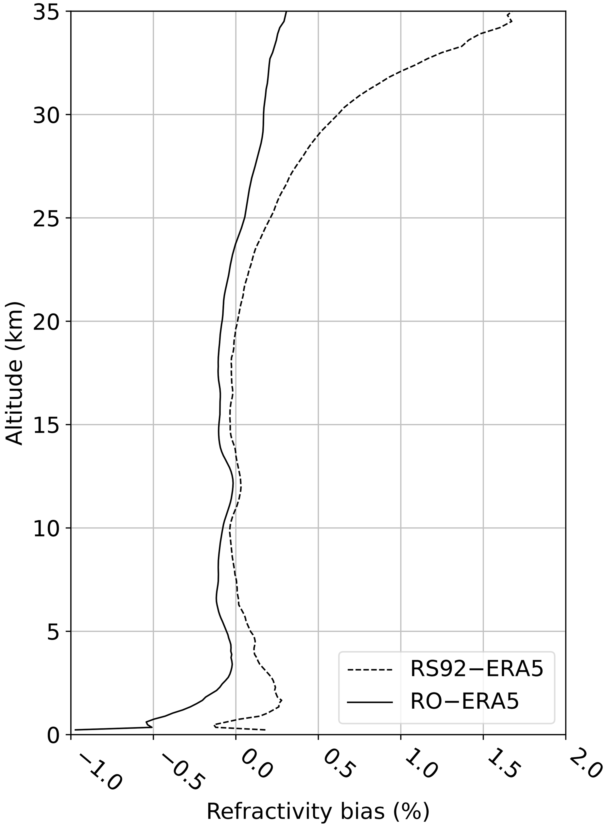
Figure 1Global biases of RS92 and RO refractivity, with ERA5 used as reference, based on all collocation triplets (collocated ERA5, RO, and RS profiles) used in this study, evaluated at the RO reference location. See also Sect. 2. Percentages are calculated relative to the mean of ERA5 forecasts.
3.4 Handling differences in vertical footprints
The three data sets differ in their vertical footprints. The RS92 radiosonde has a vertical footprint of around 50 m (Dirksen et al., 2014). This vertical footprint is increased through the interpolation to the common grid (Lewis, 2009), and through the procedure for correcting for collocation error. The RO refractivity has been shown to have a vertical footprint of about 200 m under optimal conditions in the lower troposphere (Xie et al., 2012). In the RO data used here, the processing has removed some small-scale information, and thus the RO vertical footprint is expected to be larger than 200 m. In Fig. 2 two examples of refractivities of triple collocations are shown. The plots illustrate the ability of resolving vertical structures in the middle troposphere and lower stratosphere of the three data sets. Even though the highly resolved ERA5 has 137 vertical levels, shown on the right vertical axis, it provides a somewhat smoother representation of the vertical structures compared to the RO. The RO profiles and RS92 profiles show more vertical structure than ERA5.

Figure 2Refractivity of two selected triple collocations exemplifying differences in vertical footprint. (a) ERA5, RS92, and COSMIC-1 RO (40.1∘ N, collocation distance: 18.6 km (0.2 h)) and (b) ERA5, RS92, and Metop RO (52∘ N, collocation distance: 25.5 km (1.6 h)). RS92 and ERA5 have been interpolated to the 247 RO height levels. The refractivity has been normalized by division with the mean of the ERA5 data set refractivity. The thinned refractivity levels and the 137 ERA5 model levels are printed on the right vertical axis.
Uncertainty estimates for any vertically represented variable must refer to a specified vertical footprint to be meaningful. Thus, the G3CH analysis has to be accompanied by an assessment of the vertical footprints of the data sets. In our approach the data set with the largest vertical footprint determines the common vertical footprint to be used for all three data sets. In other words, if one of the data sets does not contain information below a certain length scale, there is not enough information in the data triplet to apply the G3CH method to estimate uncertainties related to variability below that length scale.
Because ERA5 is missing some fine-scale physical features, seen in the better resolved RO and RS92 data set, we are forced to state the uncertainty on the common scale determined by ERA5. This means that the RO and RS92 data must be smoothed to match the ERA5 vertical footprint prior to the G3CH analysis. If this smoothing is omitted, the G3CH may give a biased estimate of uncertainties. By smoothing the data sets to a common scale we remove both the physical features and the errors on scales shorter than the common vertical footprint. Therefore the estimated uncertainties of RO and RS92, which are correct on the common scale found, may be viewed as lower uncertainty boundaries for these variables on their native scales. The vertical footprints of the three data sets are examined in Sect. 4.3.
In this section the G3CH results are presented, first as raw unfiltered uncertainty estimates, then with corrections for collocation mismatch (εC terms) and corrections for cross correlations due to finite vertical footprints (εX terms), to assess the uncertainty limits for each data set.
4.1 Raw uncertainty estimates
Figure 3 shows the raw estimates of the mid-latitude refractivity uncertainty expressed as error standard deviation of the three data sets, obtained by applying the G3CH directly to the raw data sets. Generally the G3CH attributes a big part of the collocation error () to the RS92 uncertainty. The reason is that the collocation is performed by interpolating ERA5 to the RO reference point, such that ERA5 and RO are closely collocated, while RS92 is chosen such that it is within 300 km of the RO reference point; thus, naturally RS92 will stand out from the two other data sets in many cases.
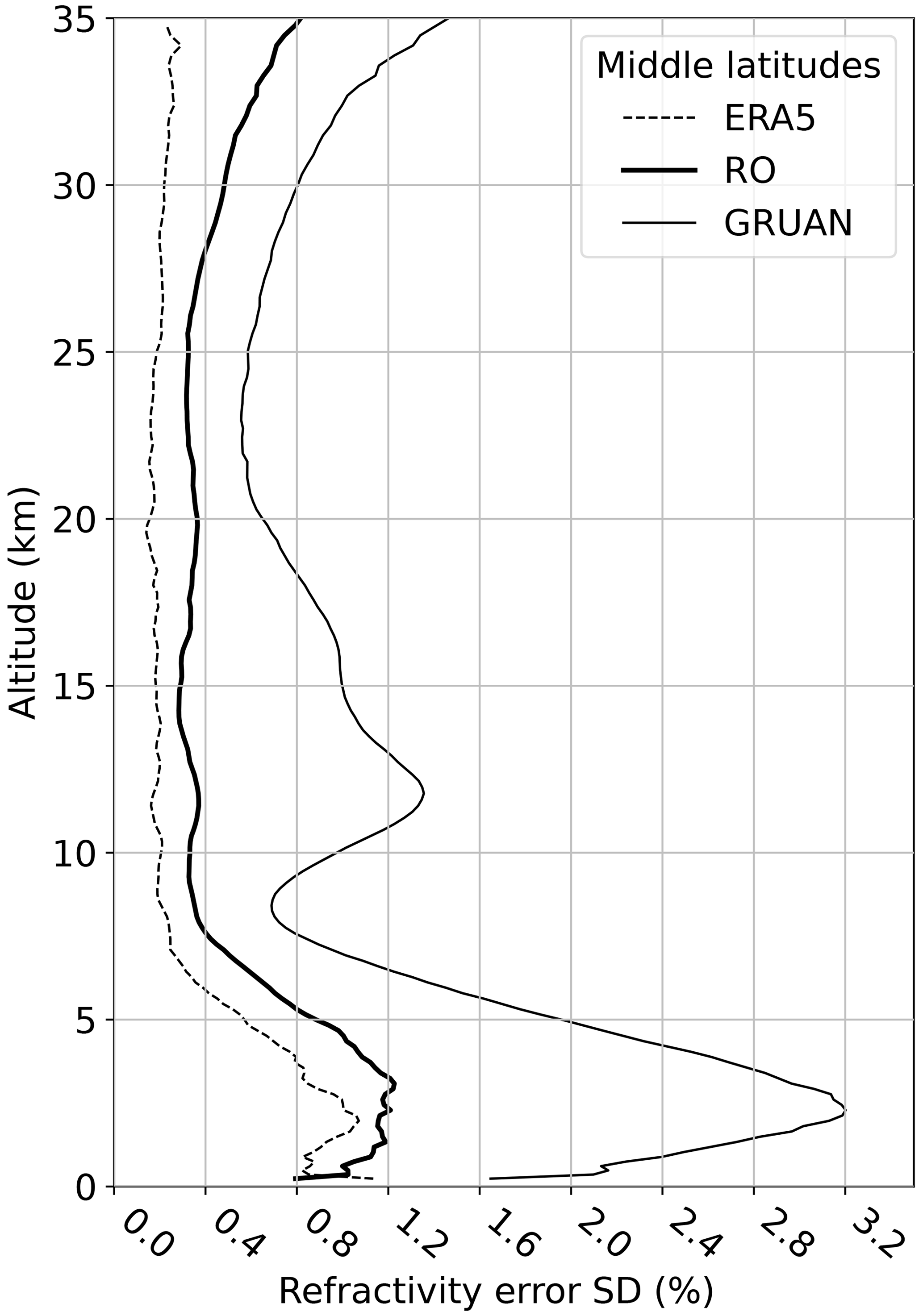
Figure 3Raw estimate of refractivity random uncertainty (standard deviation) of ERA5, RO, and RS92 at middle latitudes.
4.2 Collocation uncertainty
The most striking feature in Fig. 3 is the bulge of RS92 around the tropopause. The main part of this bulge is removed along with the collocation uncertainty by the procedure described in Sect. 3.2. We calculate the G3CH estimates of covariance matrices for a sequence of collocation criteria (between 50 and 300 km) and use these to extrapolate all covariance matrices to 0 km collocation distance, with a linear fit to the full covariance matrices as a function of the squared collocation distance. The effect of varying the temporal collocation window is small, and therefore we have excluded that from the analysis.
The impact on RS92 of changing collocation distance is shown as an example in Figs. 4 and 5 where a few examples of extrapolations are presented. The result of this procedure is summarized for all three data sets in Fig. 6. The RS92 uncertainty estimate is reduced considerably, while the uncertainty estimates for the two other data sets are slightly changed. In the subsequent analysis the 0 km estimates of covariances are used for evaluation of covariance matrices and difference terms in the G3CH equations.
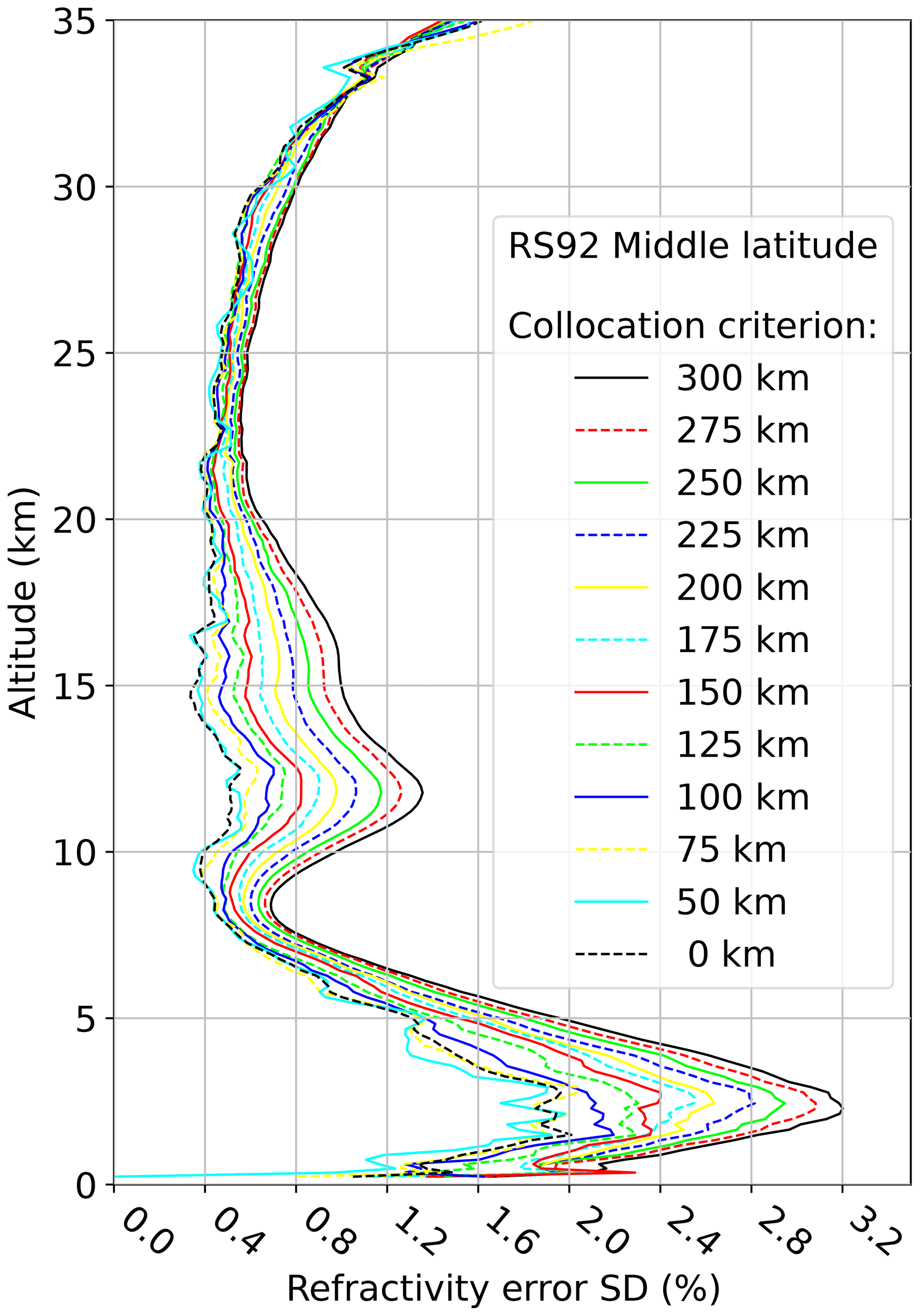
Figure 4Estimate of refractivity uncertainty (standard deviation as percent of ERA5 mean refractivity) of RS92 for a series of collocation criteria. The dashed black line shows the STDV obtained by extrapolation of the variance to zero collocation distance.

Figure 5Examples of extrapolation of refractivity error variance of RS92, i.e. diagonal elements of covariance matrix, to zero collocation criterion at five different altitudes. The variances are divided by the mean ERA5 refractivity.

Figure 63CH estimates of refractivity error standard deviations are shown for 300 and 0 km collocation criterion for each of the ERA5, RS92, and RO data sets at low (a), middle (b), and high (c) latitudes. Smoothing has not been applied.
4.3 Vertical filtering
In Fig. 7 the impact of smoothing on error standard deviations estimated with G3CH (Eq. 7) is shown for middle latitudes. The smoothing is applied as a sequence of Gaussian filters of increasing widths. For each data set, filtering has been performed, not on the data set itself, but on the two other complementary data sets (see figure legends). The idea is basically to probe the vertical footprint of one data set with two other data sets of varying vertical footprint. The G3CH analysis was performed at the sequence of such prepared triplets of data sets with increasing filter width. The impact of applying sequences of Gaussian filters is best viewed near the tropopause. We note that all variances eventually start to grow at some filter width, but the ERA5 error standard deviation drops in most cases at small filter widths, and does not start to increase until the width of the filter, applied on the RO and RS92 data, exceeds a certain threshold. We interpret this threshold as the ERA5 vertical footprint. The ERA5 vertical footprint was estimated for each altitude, as the minimum of a second-order polynomial, fitted to σERA5 as a function of filter width. These vertical footprints are plotted in Fig. 8, for middle and high latitudes. At low latitudes the result is unstable, and therefore that plot has been omitted. We use these results to identify a common ERA5 vertical footprint to be applied globally as the mean of the middle- and high-latitude vertical footprints, shown as a dashed line in Fig. 8.
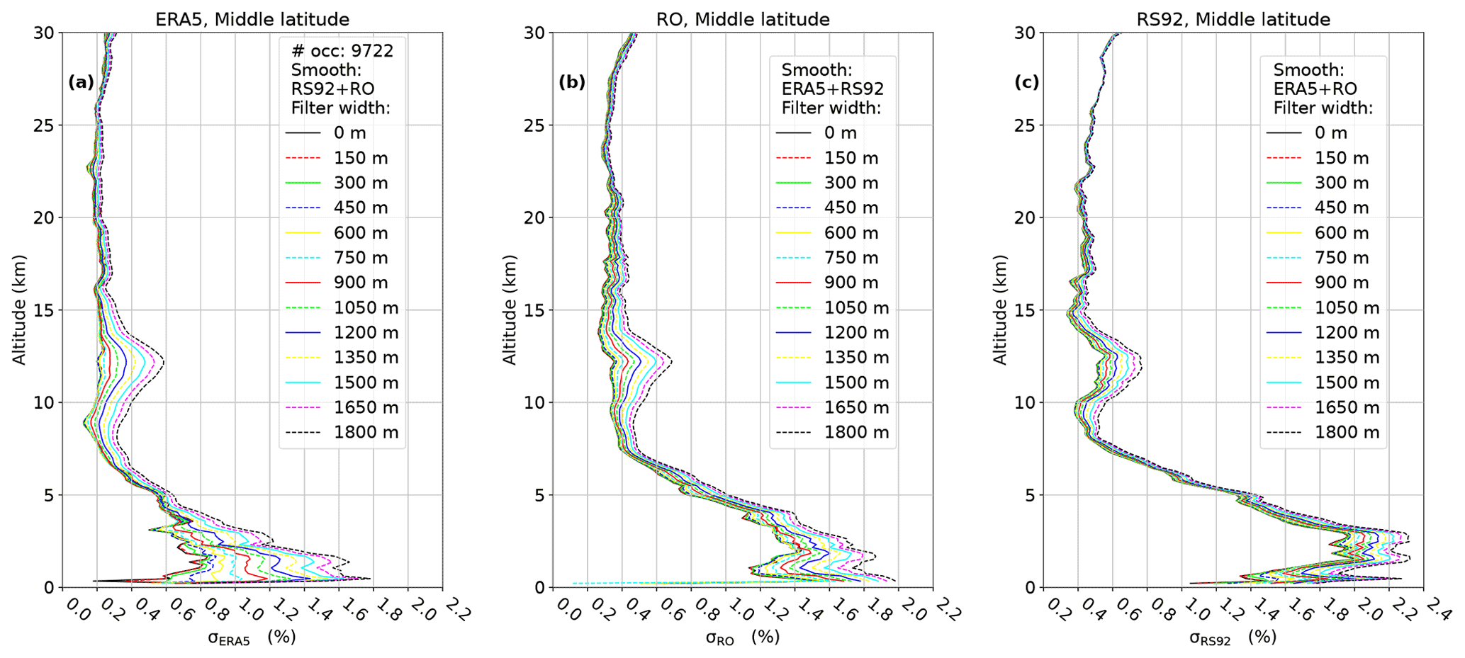
Figure 7Effect of smoothing on error standard deviations of ERA5 (a), RO (b), and RS92 (c) estimated by 3CH. Note that the x axis is shifted by 0.2 % in panel (c). All plots are for middle latitudes. The standard deviations are divided by the mean ERA5 refractivity. The filtering width is defined as 2 times the standard deviation of the Gaussian filter function. The single curves are most easily identified at a given altitude by counting the curves from one side. For each data set, the smoothing is only applied on the two other data sets.
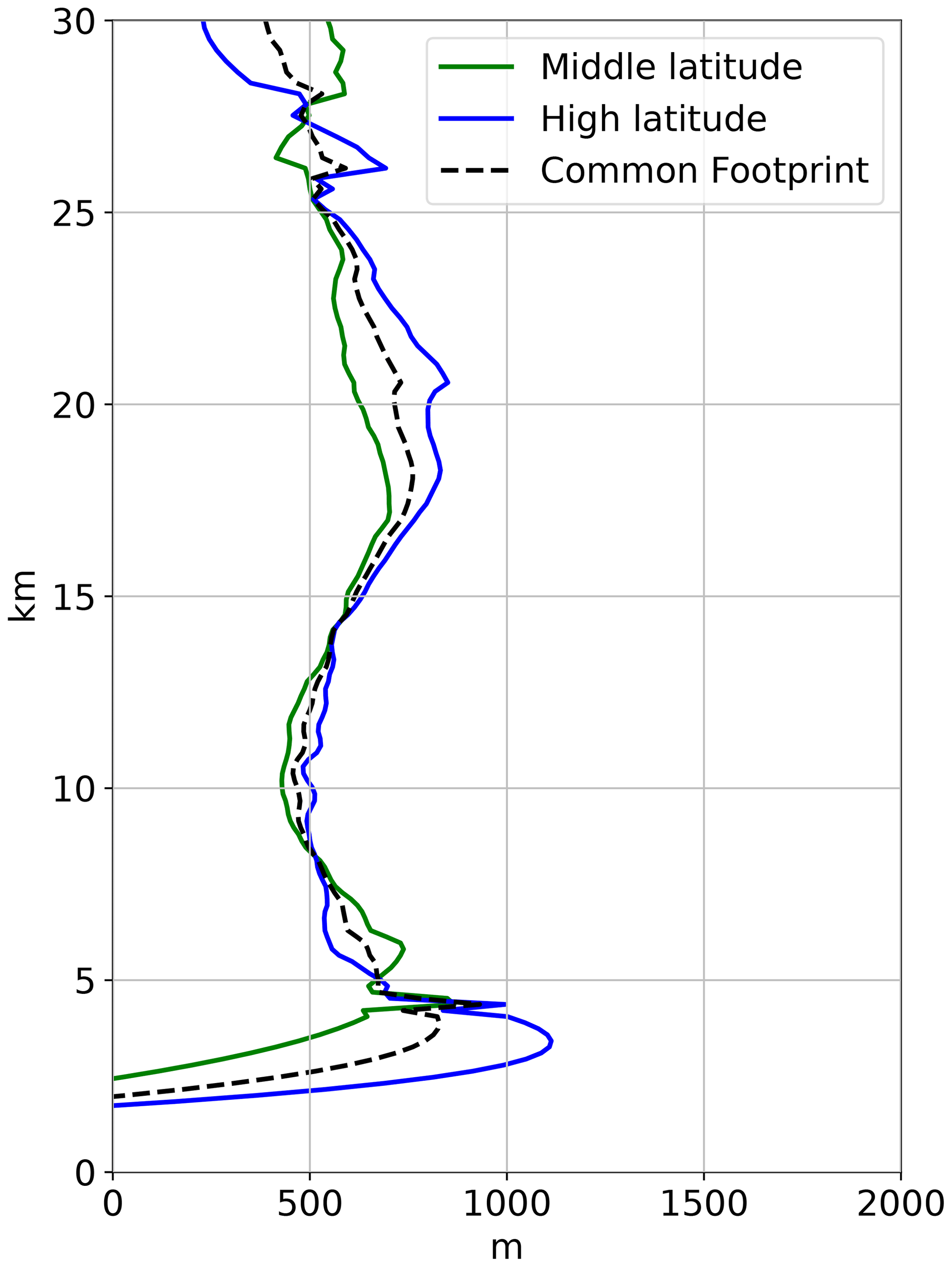
Figure 8Estimates of the ERA5 vertical footprint for middle and high latitudes. The effect of filtering of RO and RS92 on the estimated ERA5 error standard deviation, σERA5, is shown in Fig. 7a. The ERA5 vertical footprint is found for each altitude as the filter width which minimizes σERA5.
A similar analysis cannot be performed for the RO or RS92 data sets, because these appear to have small vertical footprints which happen to lie close to each other. There is not a finite filter length which minimizes the refractivity error standard deviation for RO and RS92 (the filters being applied to the complementary data sets in each case). Therefore the RO and RS92 vertical footprints cannot be inferred from these three data sets alone, but it can be concluded that their vertical footprints are smaller than the ERA5 vertical footprint since the ERA5 estimated error standard deviation decreases if either the RO or RS92 is smoothed. This is illustrated in Fig. 9: The impact of smoothing RS92 on the ERA5 variance is shown in Fig. 9a. Generally decreases as the RS92 data are brought closer to the ERA5 data by smoothing, consistent with RS92 having a smaller vertical footprint than ERA5. The RO error variance, , on the other hand increases as a result of smoothing the RS92 data (see Fig. 9b). This is consistent with the RS92 vertical footprint being close to the RO vertical footprint and the RS92 data moving closer to the ERA5 data as smoothing is applied to RS92. In Fig. 9c is seen to decrease as the RO refractivity is brought closer to ERA5 refractivity, as smoothing is applied to RO.
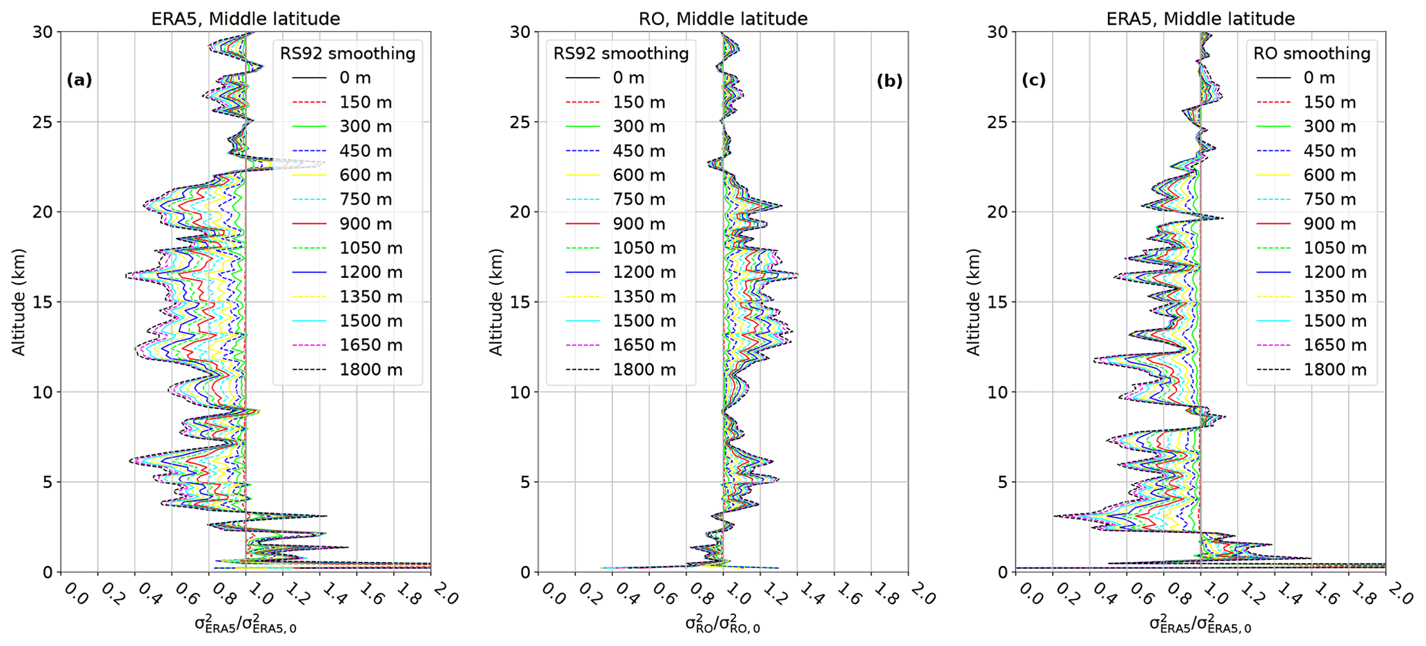
Figure 9Estimates of middle-latitude refractivity error variances based on smoothed data divided by refractivity error variance based on un-smoothed data; (a) ERA5 error variance with smoothed RS92, (b) RO error variance with smoothed RS92, and (c) ERA5 error variance with smoothed RO. The legends show the width of the different vertical Gaussian filters applied to the refractivity profiles mentioned in the legend title; e.g. in panel (a) means uncertainty estimate of ERA5, given filtering of the data set mentioned in the legend – in this case RS92, divided by the uncertainty estimate of ERA5, obtained without filtering. A total of 9722 collocated data triplets were used in the G3CH analysis for these error covariance estimates.
To estimate the final G3CH uncertainties with reference to the common vertical footprint determined by ERA5, all three raw data sets were smoothed with a Gaussian filter with the width of the ERA5 vertical footprint prior to the G3CH analysis. In Fig. 10 the final G3CH inferred uncertainties are shown for each data set for low, middle, and high latitudes. For all data sets the unfiltered uncertainty is also plotted, for later discussion.
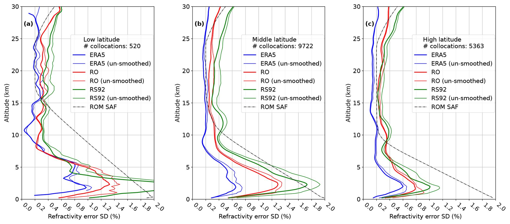
Figure 10Best estimate of refractivity uncertainties, shown as standard deviations in percent of the ERA5 refractivity for ERA5, RO, and RS92 at low (a), middle (b), and high (c) latitudes. For all data sets the uncertainty is given with reference to the ERA5 vertical footprint, which is achieved by filtering all data sets to match the ERA5 vertical footprint (thick curves). The uncertainties based on un-smoothed data are also shown (thin curves). The standard deviation estimates found have been vertically smoothed with a 10 grid points box filter.
4.4 Error covariances
In Figs. 11 and 12 the G3CH-based error covariance matrices for ERA5, RO, and RS92 are shown for rising and setting occultations for middle and high latitudes. These matrices have been calculated without any vertical filtering applied. The tropics are not shown because of insufficient number of data in that region. The fine-scale off-diagonal structures must be attributed to statistical noise, but there are certainly larger-scale vertical correlation structures especially in the RO and RS92 data.
Generally the vertical correlations are divided into two separable regimes: Close to the diagonal we see a short-range correlation with standard deviation of approximately 0.5 km, and a long-range correlation component of varying shape and amplitude. The short-scale vertical correlations are very similar for all data sets. Rising occultations are found to have larger vertical error correlations (and slightly larger standard deviation where correlations are broader) than setting occultations in this data set, which is seen when comparing panel (b) with panel (e) in Fig. 11 and panel (b) with panel (e) in Fig. 12. This is believed to be due to the ionospheric correction in the RO processing for rising occultations, where the L2 GPS signal is often not available below 20 km, and extrapolation from above is necessary. In the CDR v1.0 data set, it is in particular the rising occultations for Metop after instrument firmware upgrades in 2013 that suffer from missing L2 data below 20 km (Gleisner et al., 2020), and consequently there are broader vertical error correlations in the retrieved refractivity profiles for Metop after 2013 (not shown).
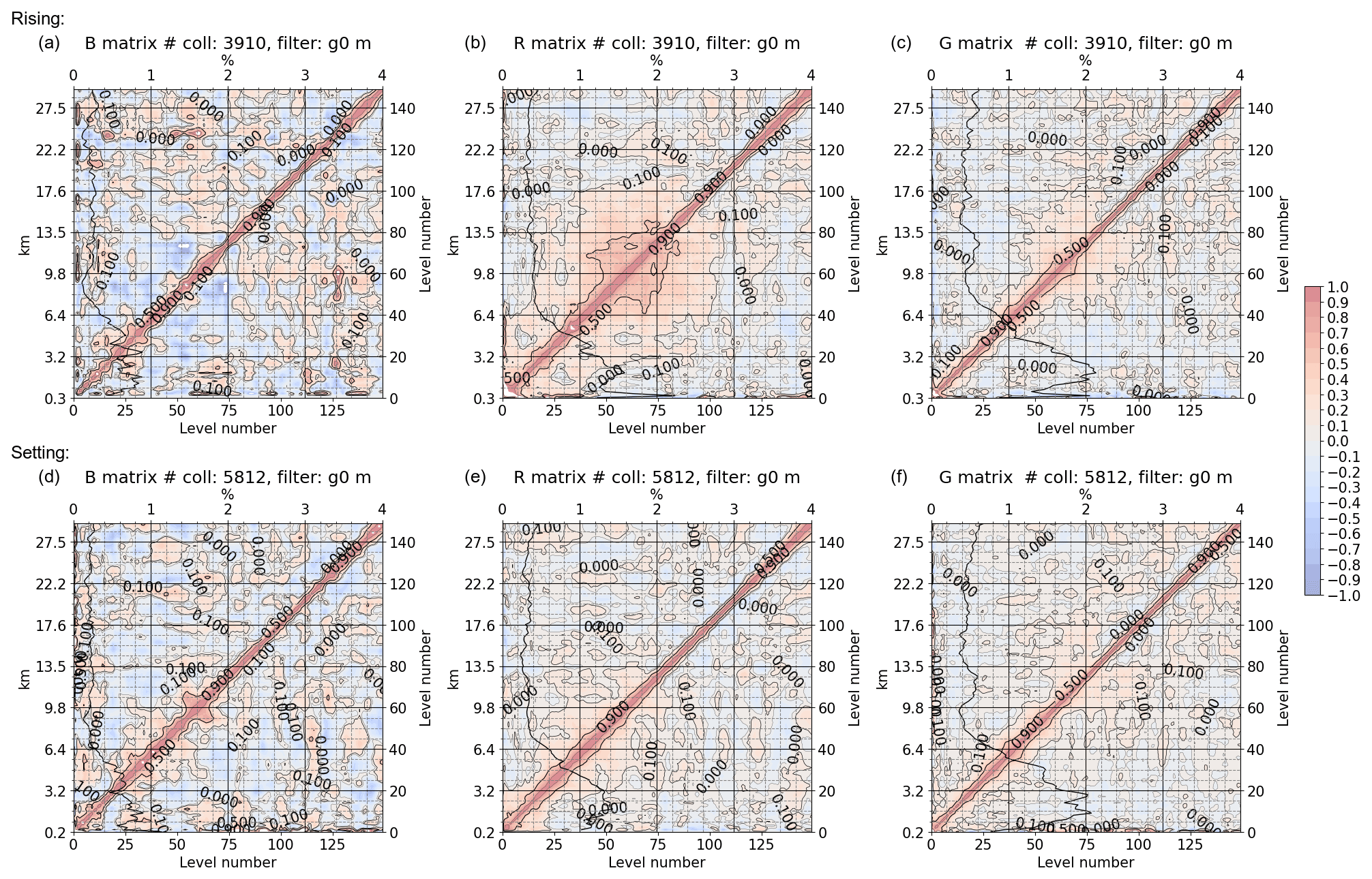
Figure 11G3CH estimate of ERA5 (a, d), RO (b, e), and RS92 (c, f) refractivity vertical error covariance matrices at middle latitude. Rising occultations (a–c) and setting occultations (d–f). The covariance matrices are plotted as correlation matrices (diagonal =1) with superimposed standard deviation as a function of height (black line), plotted on the left and upper axes. The standard deviation is given as percent of the mean ERA5 forecast refractivity. The covariance matrices have been truncated at 30 km where the RS92 data sparseness starts to destabilize the results. A total of 9722 collocated profile triplets were used for these covariance estimates. For these estimates no smoothing was applied on any of the data sets.
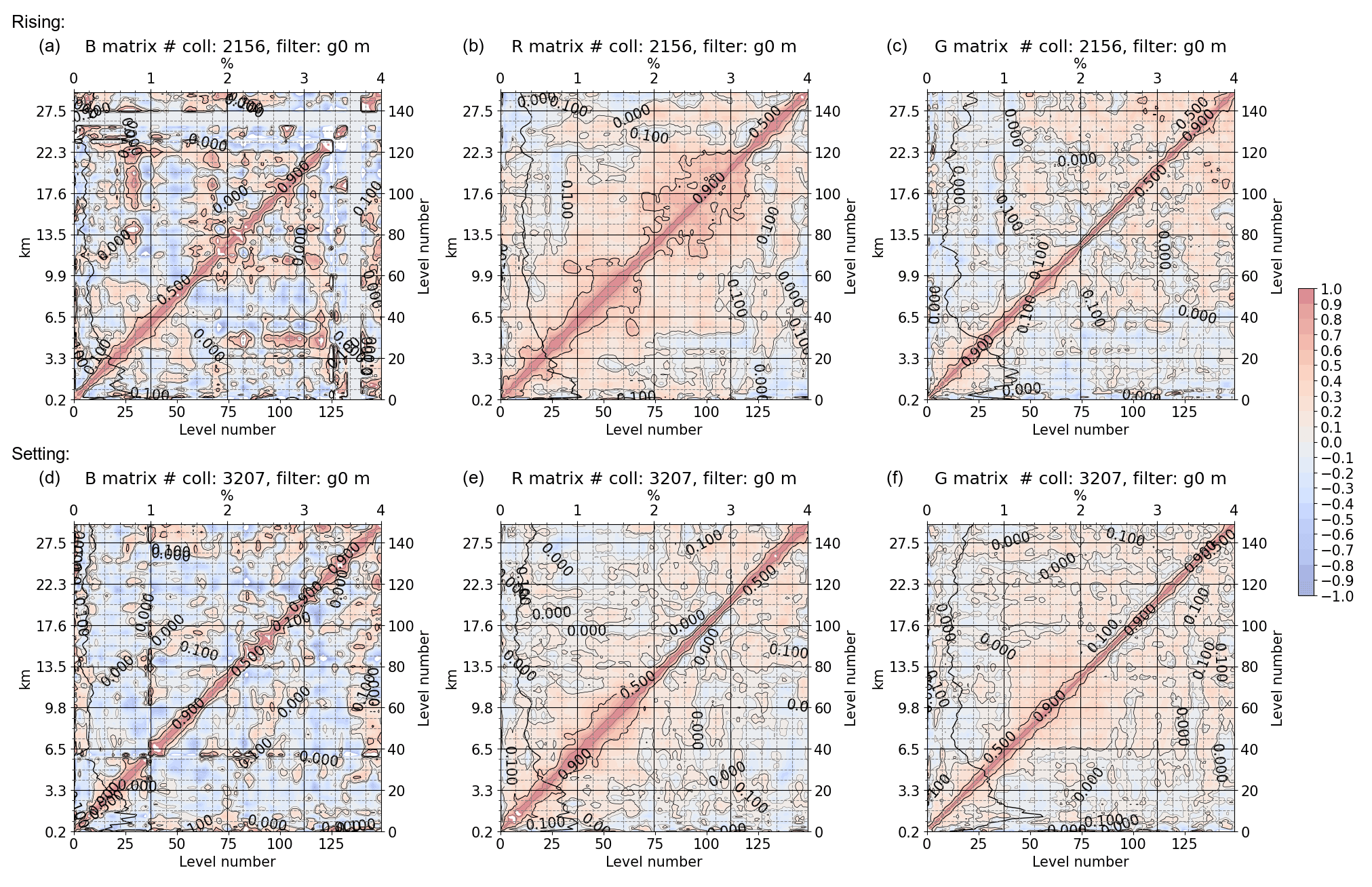
Figure 12Same as in Fig. 11, but for high latitudes.
It is worth noting that the estimated vertical correlations of RS92 are larger for setting than for rising RO at high latitudes, especially between 6 and 22 km. Thus the G3CH fails to give an independent estimate of the RS92 correlations. The RS92 is expected to have long-ranging vertical correlations due to corrections implemented in the GRUAN processing, but the G3CH fails to attribute these correctly when strong long-range correlations are also present in the RO data. The estimated RS92 diagonals (standard deviations superimposed vertically on correlation matrices) seem reasonably consistent for rising and setting occultations.
The relative magnitude of the off-diagonal covariance components can also be viewed in Fig. 13: Here the vertical error correlation function of RO refractivity is exemplified for two heights, approximately 5 and 20 km, at low, middle, and high latitudes. The correlation functions are slices of the RO refractivity error correlation matrix at these altitudes. For instance at high latitude there are pronounced long-range correlations at these two heights. In the tropics the data are too sparse to get an estimate of the correlation function. In Fig. 13 the dashed curves show the three kilometre exponential correlation which is assumed in the current ROM SAF 1D-Var analysis (ROM SAF, 2021b). Given that the finer correlation structures, around the 1 km scale, are influenced by sparseness of data, the current correlation function appears to be reasonably adequate at high latitudes at the selected altitudes. At middle latitudes there is a potential for decreasing the error correlation length in future applications.
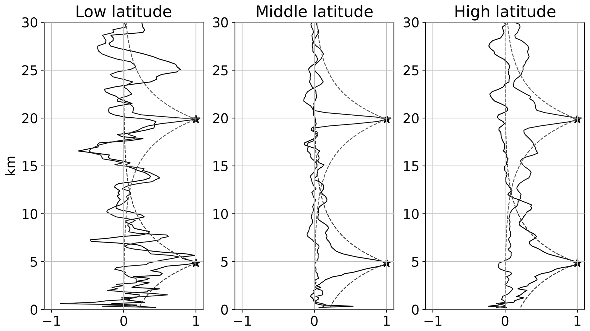
Figure 13Estimate of RO vertical error correlations at approximately 5 and 20 km for low, middle, and high latitudes (full curves). The dashed lines show exponential correlation with three kilometre decay length. No smoothing was applied on any of the data sets before the G3CH was applied.
It is evident from the results in Sect. 4.3 that uncertainty estimates for a data set must be stated with reference to scale in space and time. We choose for all data sets to report the estimated uncertainty boundaries with reference to the estimated vertical footprint of the ERA5 data set. We identified the vertical footprint of ERA5 for a range of altitudes, and used these to find RO uncertainties in Fig. 10.
The unfiltered G3CH RO uncertainty estimates, also seen in Fig. 10, include uncertainty associated with fluctuations on shorter scales than the ERA5 vertical footprint. The unfiltered uncertainties are overestimated because they will include physical variability, falsely attributed as errors. We cannot quantify the native vertical footprints of RO and RS92, but it can be assumed that the unfiltered uncertainty estimates mark upper boundaries for their uncertainties evaluated with reference to the native vertical footprint.
The estimated uncertainties of RO in the lower stratosphere are only slightly above 0.2 %, the theoretical estimates found in Kursinski et al. (1997). Empirical uncertainty estimates have previously been analysed, for instance by Rieckh and Anthes (2018) and Scherllin-Pirscher et al. (2011). In the empirical uncertainty analysis study by Scherllin-Pirscher et al. (2011), the refractivity uncertainty is found to be 0.35 % in the lower stratosphere. Scherllin-Pirscher et al. (2011) used RO data in combination with ECMWF analysis, and were therefore confined to make assumptions about mutual correlation and partitioning of uncertainties among the two data sets. By combining three independent data sets in a 3CH analysis such assumptions may be avoided, and consequently one is able to decrease the uncertainty estimates.
The RO uncertainty in the Upper Troposphere–Lower Stratosphere (UTLS), where the uncertainty estimates are at a minimum, does not vary much with latitude, except for a small increase at the tropopause. The structure of the uncertainty profiles is quite similar for all latitudes. The increase of uncertainty in the troposphere is smaller at high latitude, but the crossover between high and low uncertainty happens at approximately the same altitude, 5–7 km, for all latitudes. For the tropics, the noisy uncertainty estimates, due to an insufficient number of data, do not allow us to safely read a minimum above the tropopause from Fig. 10, but there is an indication of uncertainty almost down to 0.2 % even between 7 and 10 km, well below the tropical tropopause layer.
In Rieckh et al. (2021) the 3CH is applied to multiple triplets of RO data and different model refractivity data. Overall their uncertainty estimates are much higher, for instance 0.55 % in the UTLS. This may be partly due to the high noise level of the analysed RO data (COSMIC-1 and COSMIC-2). But the data sets used by Rieckh et al. (2021) are less well suited to 3CH analysis than the data sets used here, because the errors of the ERA5 analysis fields used must be expected to be correlated with errors of other data sets, leading to a biased estimate of 3CH uncertainties. The models applied have larger vertical footprint than the RS92 radiosonde data used here, and this will tend to yield an overestimate of RO uncertainties, which is indeed seen in Rieckh et al. (2021). Their results show apparent uncertainty maxima near the tropopause, as must be anticipated according to our analysis of the impact of vertical footprints in Sect. 4.3.
In the theoretical uncertainty analysis study by Kursinski et al. (1997) the refractivity uncertainty in the lower troposphere tangents is 1 %, which is a little lower than the G3CH estimate at middle latitudes, but quite consistent with the G3CH estimate at high latitudes. The Kursinski et al. (1997) estimate is dominated by the contribution from representativeness uncertainty arising from horizontal gradients along the ray path up to 30 km, i.e. the contribution from the spherical symmetry assumption to the uncertainty. Retrospectively seen, Kursinski et al. (1997) may have underestimated the horizontal gradients in the troposphere since the effect of horizontal variability was estimated from a model with 40 km horizontal resolution. In a later study by Steiner and Kirchengast (2005), even lower refractivity uncertainty estimates are obtained, with a coarser model (60 km resolution and 50 vertical levels). Steiner and Kirchengast (2005) find down to 0.1 % refractivity uncertainty in the UTLS.
The estimation of error correlation matrices with G3CH is a novelty introduced in the present study. The method is able to detect expected differences between rising and setting RO long-range vertical error correlations, and long-range correlations are also seen in RS92 data. The vertical correlation estimates have limitations since the estimate of long-range vertical error correlations of RS92 seems to be dependent on whether the RO data used represent rising or setting occultations. However, this inaccuracy seems relatively small compared to the difference between the RO vertical error correlation estimates found and the vertical error correlation estimates currently used in RO 1D-Var retrievals, and therefore the correlation estimates will be useful in this context. Especially at middle latitudes there is a potential for decreasing the vertical error correlation length in future applications.
The analysis of G3CH presented here may have consequences for uncertainty parameterization in retrieval and assimilation of RO refractivity. In particular the estimates of RO refractivity uncertainty reveal a potential for deflating tropospheric refractivity uncertainty in the ROM SAF 1D-Var configuration. A reduction of assumed refractivity uncertainty is of particular interest in the troposphere, where it can improve the information content of water vapour retrievals. There is a need to establish tropospheric water vapour climate data records for climate research, for instance as expressed in the objectives of the GEWEX water vapour assessment (G-VAP; Schröder et al., 2018). The results presented here promise a reduction in the uncertainty of RO-based tropospheric water vapour retrieval.
The collocation-corrected G3CH random uncertainty estimate provides full refractivity error covariance matrices for three independent data sets. The method was applied to collocated refractivity profiles from ERA5 forecasts, RO, and radiosondes.
The RO refractivity uncertainty is between 0.2 % and 0.6 % in the UTLS at between 8 and 25 km at middle and high latitudes, and between 0.2 % and 1.4 % below 8 km. The G3CH method presented here also yields estimates of the vertical error covariance matrices for refractivity.
The achieved refractivity uncertainty estimates are lower than empirically determined uncertainties previously reported in the literature. The results can be used to model uncertainty assumptions used in NWP data assimilation and in 1D-Var calculations of atmospheric temperature and specific humidity based on RO refractivity data.
The analysis was performed in Jupyter Notebook. The code is kept in an internal git repository at the Danish Meteorological Institute. It is available from the corresponding author upon request.
The RO refractivity profiles and interpolated ERA5 temperature and humidity profiles on model levels (including surface pressure) are available at the ROM SAF web-page https://www.romsaf.org (last access: October 2022; Gleisner et al., 2019, 2022). The GRUAN atmospheric profiles are available at the GRUAN web-page (Sommer et al., 2012).
The supplement related to this article is available online at: https://doi.org/10.5194/amt-15-6243-2022-supplement.
JKN put together (and partly invented) the method, performed the analysis, and is the main author of the paper. SS, KBL, and HG contributed with substantial reformulations of every part of the manuscript, through multiple iterations, which led to changes in the basic rationale of the paper.
The contact author has declared that none of the authors has any competing interests.
Publisher’s note: Copernicus Publications remains neutral with regard to jurisdictional claims in published maps and institutional affiliations.
This article is part of the special issue “Analysis of atmospheric water vapour observations and their uncertainties for climate applications (ACP/AMT/ESSD/HESS inter-journal SI)”. It is not associated with a conference.
This work was carried out as part of EUMETSAT's Radio Occultation Meteorology Satellite Application Facility (ROM SAF) which is a decentralised operational RO processing center under EUMETSAT. Johannes K. Nielsen, Hans Gleisner, Stig Syndergaard, and Kent B. Lauritsen are members of the ROM SAF. We wish to thank the reviewers John Eyre, Paul Poli and the third anonymous reviewer for helping to improve the paper.
This research has been supported by the European Organisation for the Exploitation of Meteorological Satellites (EUMETSAT).
This paper was edited by Chunlüe Zhou and reviewed by John Eyre, Paul Poli, and one anonymous referee.
Barnes, J.: Atomic Timekeeping and the Statistics of Precision Signal Generators, Proc. IEEE, 54, 207–220, https://doi.org/10.1109/PROC.1966.4633, 1966. a
Bormann, N., Bonavita, M., Dragani, R., Eresmaa, R., Matricardi, M., and McNally, A.: Enhancing the Impact of IASI Observations through an Updated Observation-Error Covariance Matrix, Q. J. Roy. Meteor. Soc., 142, 1767–1780, https://doi.org/10.1002/qj.2774, 2016. a, b
Desroziers, G., Berre, L., Chapnik, B., and Poli, P.: Diagnosis of Observation, Background and Analysis-Error Statistics in Observation Space, Q. J. Roy. Meteor. Soc., 131, 3385–3396, https://doi.org/10.1256/qj.05.108, 2005. a
Dirksen, R. J., Sommer, M., Immler, F. J., Hurst, D. F., Kivi, R., and Vömel, H.: Reference quality upper-air measurements: GRUAN data processing for the Vaisala RS92 radiosonde, Atmos. Meas. Tech., 7, 4463–4490, https://doi.org/10.5194/amt-7-4463-2014, 2014. a, b
Gleisner, H., Lauritsen, K. B., Nielsen, J. K., and Syndergaard, S.: Evaluation of the 15-year ROM SAF monthly mean GPS radio occultation climate data record, Atmos. Meas. Tech., 13, 3081–3098, https://doi.org/10.5194/amt-13-3081-2020, 2020. a, b
Gleisner, H., Bækgaard Lauritsen, K. B., Nielsen, J. K., and Syndergaard, S.: ROM SAF Radio Occultation Climate Data Record v1.0, GRM-29-R1 (2019), for 2006 to 2016, EUMETSAT [data set], https://doi.org/10.15770/EUM_SAF_GRM_0002, 2019. a, b
Gleisner, H., Bækgaard Lauritsen, K. B., Nielsen, J. K., and Syndergaard, S.: ROM SAF Radio Occultation Interim Climate Data Record v1.0, GRM-29-I1 (2019), for 2017 to 2020, EUMETSAT [data set], https://doi.org/10.15770/EUM_SAF_GRM_0006, 2022. a, b
Gray, J. and Allan, D.: A Method for Estimating the Frequency Stability of an Individual Oscillator, in: 28th Annual Symposium on Frequency Control, Atlantic City, NJ, USA, 29–31 May 1974, 243–246, https://doi.org/10.1109/FREQ.1974.200027, 1974. a
Grubbs, F. E.: On Estimating Precision of Measuring Instruments and Product Variability, J. Am. Stat. Assoc., 43, 243–264, 1948. a, b
Healy, S. B. and Eyre, J. R.: Retrieving Temperature, Water Vapour and Surface Pressure Information from Refractive-Index Profiles Derived by Radio Occultation: A Simulation Study, Q. J. Roy. Meteor. Soc., 126, 1661–1683, https://doi.org/10.1002/qj.49712656606, 2000. a
Hersbach, H., Bell, B., Berrisford, P., Hirahara, S., Horányi, A., Muñoz-Sabater, J., Nicolas, J., Peubey, C., Radu, R., Schepers, D., Simmons, A., Soci, C., Abdalla, S., Abellan, X., Balsamo, G., Bechtold, P., Biavati, G., Bidlot, J., Bonavita, M., Chiara, G. D., Dahlgren, P., Dee, D., Diamantakis, M., Dragani, R., Flemming, J., Forbes, R., Fuentes, M., Geer, A., Haimberger, L., Healy, S., Hogan, R. J., Hólm, E., Janisková, M., Keeley, S., Laloyaux, P., Lopez, P., Lupu, C., Radnoti, G., de Rosnay, P., Rozum, I., Vamborg, F., Villaume, S., and Thépaut, J.-N.: The ERA5 Global Reanalysis, Q. J. Roy. Meteor. Soc., 146, 1999–2049, https://doi.org/10.1002/qj.3803, 2020. a, b
Hollingsworth, A. and Lönnberg, P.: The Statistical Structure of Short-Range Forecast Errors as Determined from Radiosonde Data. Part I: The Wind Field, Tellus A, 38A, 111–136, https://doi.org/10.1111/j.1600-0870.1986.tb00460.x, 1986. a
Joint Committee for Guides in Metrology: JCGM 100:2008, GUM 1995 with minor corrections, Evaluation of measurement data – Guide to the expression of uncertainty in measurement, https://www.bipm.org/documents/20126/2071204/JCGM_100_2008_E.pdf, last access: September 2008. a
Kursinski, E. R., Hajj, G. A., Schofield, J. T., Linfield, R. P., and Hardy, K. R.: Observing Earth's Atmosphere with Radio Occultation Measurements Using the Global Positioning System, J. Geophys. Res.-Atmos., 102, 23429–23465, https://doi.org/10.1029/97JD01569, 1997. a, b, c, d
Kursinski, E. R., Healy, S. B., and Romans, L. J.: Initial Results of Combining GPS Occultations with ECMWF Global Analyses within a 1DVar Framework, Earth Planets Space, 52, 885–892, https://doi.org/10.1186/BF03352301, 2000. a
Levine, J.: Introduction to Time and Frequency Metrology, Rev. Sci. Instrum., 70, 2567, https://doi.org/10.1063/1.1149844, 1999. a
Lewis, H.: GRAS SAF Report 08 ROPP Thinner Algorithm, EUMETSAT, Tech. Rep. SAF/GRAS/METO/REP/GSR/008, https://www.romsaf.org/general-documents/gsr/gsr_08.pdf, last access: June 2009. a, b
Merchant, C. J., Holl, G., Mittaz, J. P. D., and Woolliams, E. R.: Radiance Uncertainty Characterisation to Facilitate Climate Data Record Creation, Remote Sens., 11, 474, https://doi.org/10.3390/rs11050474, 2019. a
O'Carroll, A. G., Eyre, J. R., and Saunders, R. W.: Three-Way Error Analysis between AATSR, AMSR-E, and In Situ Sea Surface Temperature Observations, J. Atmos. Ocean. Tech., 25, 1197–1207, https://doi.org/10.1175/2007JTECHO542.1, 2008. a
Rieckh, T. and Anthes, R.: Evaluating two methods of estimating error variances using simulated data sets with known errors, Atmos. Meas. Tech., 11, 4309–4325, https://doi.org/10.5194/amt-11-4309-2018, 2018. a, b
Rieckh, T., Sjoberg, J. P., and Anthes, R. A.: The Three-Cornered Hat Method for Estimating Error Variances of Three or More Atmospheric Datasets. Part II: Evaluating Radio Occultation and Radiosonde Observations, Global Model Forecasts, and Reanalyses, J. Atmos. Ocean. Tech., 38, 1777–1796, https://doi.org/10.1175/JTECH-D-20-0209.1, 2021. a, b, c, d
ROM SAF: The Radio Occultation Processing Package (ROPP) Forward Model Module User Guide, EUMETSAT ROM SAF, Tech. Rep. SAF/ROM/METO/UG/ROPP/006, https://www.romsaf.org/romsaf_ropp_ug_fm.pdf, last access: December 2021a. a
ROM SAF: Algorithm Theoretical Baseline Document: Level 2B and 2C 1D-Var Products, Version 4.3, EUMETSAT ROM SAF, Tech. Rep. SAF-/ROM-/DMI-/ALG-/1DV-/002, http://www.romsaf.org (last access: October 2021), 2021b. a, b
Scherllin-Pirscher, B., Steiner, A. K., Kirchengast, G., Kuo, Y.-H., and Foelsche, U.: Empirical analysis and modeling of errors of atmospheric profiles from GPS radio occultation, Atmos. Meas. Tech., 4, 1875–1890, https://doi.org/10.5194/amt-4-1875-2011, 2011. a, b, c
Schröder, M., Lockhoff, M., Fell, F., Forsythe, J., Trent, T., Bennartz, R., Borbas, E., Bosilovich, M. G., Castelli, E., Hersbach, H., Kachi, M., Kobayashi, S., Kursinski, E. R., Loyola, D., Mears, C., Preusker, R., Rossow, W. B., and Saha, S.: The GEWEX Water Vapor Assessment archive of water vapour products from satellite observations and reanalyses, Earth Syst. Sci. Data, 10, 1093–1117, https://doi.org/10.5194/essd-10-1093-2018, 2018. a
Semane, N., Anthes, R., Sjoberg, J., Healy, S., and Ruston, B.: Comparison of Desroziers and Three-Cornered Hat Methods for Estimating COSMIC-2 Bending Angle Uncertainties, J. Atmos. Ocean. Tech., 39, 929–939, https://doi.org/10.1175/JTECH-D-21-0175.1, 2022. a
Sjoberg, J. P., Anthes, R. A., and Rieckh, T.: The Three-Cornered Hat Method for Estimating Error Variances of Three or More Atmospheric Data Sets – Part I: Overview and Evaluation, J. Atmos. Ocean. Tech., 38, 555–572, https://doi.org/10.1175/JTECH-D-19-0217.1, 2020. a, b, c
Sommer, M., Dirksen, R., and Immler, F.: RS92 GRUAN Data Product Version 2 (RS92-GDP.2), GRUAN [data set], https://doi.org/10.5676/GRUAN/RS92-GDP.2, 2012. a, b
Steiner, A. K. and Kirchengast, G.: Error Analysis for GNSS Radio Occultation Data Based on Ensembles of Profiles from End-to-End Simulations, J. Geophys. Res.-Atmos., 110, D15307, https://doi.org/10.1029/2004JD005251, 2005. a, b
Steiner, A. K., Ladstädter, F., Ao, C. O., Gleisner, H., Ho, S.-P., Hunt, D., Schmidt, T., Foelsche, U., Kirchengast, G., Kuo, Y.-H., Lauritsen, K. B., Mannucci, A. J., Nielsen, J. K., Schreiner, W., Schwärz, M., Sokolovskiy, S., Syndergaard, S., and Wickert, J.: Consistency and structural uncertainty of multi-mission GPS radio occultation records, Atmos. Meas. Tech., 13, 2547–2575, https://doi.org/10.5194/amt-13-2547-2020, 2020. a
Syndergaard, S., Kursinski, E. R., Herman, B. M., Lane, E. M., and Flittner, D. E.: A Refractive Index Mapping Operator for Assimilation of Occultation Data, Mon. Weather Rev., 133, 2650–2668, https://doi.org/10.1175/MWR3001.1, 2005. a
Xie, F., Wu, D. L., Ao, C. O., Mannucci, A. J., and Kursinski, E. R.: Advances and limitations of atmospheric boundary layer observations with GPS occultation over southeast Pacific Ocean, Atmos. Chem. Phys., 12, 903–918, https://doi.org/10.5194/acp-12-903-2012, 2012. a
three-cornered hat: Instead of calculating uncertainties from assumed knowledge about the observation method, uncertainties and error correlations are estimated statistically from tree independent observation series, measuring the same variable. The results are useful for future estimation of atmospheric-specific humidity from the bending of radio waves.