the Creative Commons Attribution 4.0 License.
the Creative Commons Attribution 4.0 License.
 | 29 Aug 2023
Retrieving 3D distributions of atmospheric particles using Atmospheric Tomography with 3D Radiative Transfer – Part 2: Local optimization
Aviad Levis
Larry Di Girolamo
Vadim Holodovsky
Linda Forster
Anthony B. Davis
Yoav Y. Schechner
Our global understanding of clouds and aerosols relies on the remote sensing of their optical, microphysical, and macrophysical properties using, in part, scattered solar radiation. Current retrievals assume clouds and aerosols form plane-parallel, homogeneous layers and utilize 1D radiative transfer (RT) models. These assumptions limit the detail that can be retrieved about the 3D variability in the cloud and aerosol fields and induce biases in the retrieved properties for highly heterogeneous structures such as cumulus clouds and smoke plumes. In Part 1 of this two-part study, we validated a tomographic method that utilizes multi-angle passive imagery to retrieve 3D distributions of species using 3D RT to overcome these issues. That validation characterized the uncertainty in the approximate Jacobian used in the tomographic retrieval over a wide range of atmospheric and surface conditions for several horizontal boundary conditions. Here, in Part 2, we test the algorithm's effectiveness on synthetic data to test whether the retrieval accuracy is limited by the use of the approximate Jacobian. We retrieve 3D distributions of a volume extinction coefficient (σ3D) at 40 m resolution from synthetic multi-angle, mono-spectral imagery at 35 m resolution derived from stochastically generated cumuliform-type clouds in (1 km)3 domains. The retrievals are idealized in that we neglect forward-modelling and instrumental errors, with the exception of radiometric noise; thus, reported retrieval errors are the lower bounds. σ3D is retrieved with, on average, a relative root mean square error (RRMSE) < 20 % and bias < 0.1 % for clouds with maximum optical depth (MOD) < 17, and the RRMSE of the radiances is < 0.5 %, indicating very high accuracy in shallow cumulus conditions. As the MOD of the clouds increases to 80, the RRMSE and biases in σ3D worsen to 60 % and −35 %, respectively, and the RRMSE of the radiances reaches 16 %, indicating incomplete convergence. This is expected from the increasing ill-conditioning of the inverse problem with the decreasing mean free path predicted by RT theory and discussed in detail in Part 1. We tested retrievals that use a forward model that is not only less ill-conditioned (in terms of condition number) but also less accurate, due to more aggressive delta-M scaling. This reduces the radiance RRMSE to 9 % and the bias in σ3D to −8 % in clouds with MOD ∼ 80, with no improvement in the RRMSE of σ3D. This illustrates a significant sensitivity of the retrieval to the numerical configuration of the RT model which, at least in our circumstances, improves the retrieval accuracy. All of these ensemble-averaged results are robust in response to the inclusion of radiometric noise during the retrieval. However, individual realizations can have large deviations of up to 18 % in the mean extinction in clouds with MOD ∼ 80, which indicates large uncertainties in the retrievals in the optically thick limit. Using less ill-conditioned forward model tomography can also accurately infer optical depths (ODs) in conditions spanning the majority of oceanic cumulus fields (MOD < 80), as the retrieval provides ODs with bias and RRMSE values better than −8 % and 36 %, respectively. This is a significant improvement over retrievals using 1D RT, which have OD biases between −30 % and −23 % and RRMSE between 29 % and 80 % for the clouds used here. Prior information or other sources of information will be required to improve the RRMSE of σ3D in the optically thick limit, where the RRMSE is shown to have a strong spatial structure that varies with the solar and viewing geometry.
- Article
(5284 KB) - Full-text XML
- Companion paper
- BibTeX
- EndNote


Remote-sensing retrievals of cloud and aerosol properties are important contributors to our understanding of cloud and aerosol processes and constraining the emergent behaviour of these processes on Earth's climate (Bellouin et al., 2020; Sherwood et al., 2020). As atmospheric modelling has become more complex, there has been an increased demand for high-quality observations to constrain the uncertain processes within the models and inform model development (Morrison et al., 2020). New observational techniques are required that can provide robust statistics of small-scale, spatially resolved cloud and aerosol microphysical parameters, so that their controlling processes can be constrained in both high- and low-resolution modelling.
In Part 1 of this study (Loveridge et al., 2023a), we described a remote-sensing retrieval technique with the potential to meet these needs by providing 3D instantaneous snapshots of volumetric properties of the atmosphere at the resolution of passive imagery. Our method uses multi-angle imagery and the spherical harmonics discrete ordinates method (SHDOM; Evans, 1998) for modelling 3D radiative transfer (RT) to constrain the 3D properties of atmospheric particles, such as effective particle radius and mass concentration (Levis et al., 2020; Tzabari et al., 2022), in a process called tomography (Arridge and Schotland, 2009; Martin et al., 2014). Our retrieval algorithm for the tomography problem directly builds upon earlier work in making such retrievals tangible and computationally efficient through the use of approximate Jacobians of 3D radiative transfer that enable the use of efficient gradient-based local optimization methods (Levis et al., 2015, 2017, 2020). We have made our method publicly available in the software package called Atmospheric Tomography with 3D Radiative Transfer (AT3D; Loveridge et al., 2022), which was developed from the research software used in Levis et al. (2015, 2017, 2020) called pySHDOM.
Our tomographic algorithm retrieves 3D properties and makes use of 3D RT. In doing so, it relaxes the twin assumptions of independent pixels and homogeneous plane-parallel clouds that cause significant biases in operational retrievals of cloud microphysical properties (Marshak et al., 2006; Kato and Marshak, 2009; Zhang et al., 2012; Lebsock and Su, 2014; Ahn et al., 2018; Fu et al., 2019; Painemal et al., 2021; Fu et al., 2022). Another key advantage of the method is that it does not rely on expensive active remote sensing for retrieving volumetric information, as in other methods (Fielding et al., 2014). Instead, the method only relies on relatively inexpensive passive imaging in the solar part of the spectrum. It thereby enables wide swath widths and high-resolution retrievals with high signal-to-noise ratio and high sensitivity to scattering particles in the size range of atmospheric clouds and aerosols (Dubovik et al., 2011; King and Vaughan, 2012; Ewald et al., 2021). These benefits position the tomographic retrieval as a means of filling the observational gap that exists for the highly heterogeneous fields of cumulus clouds that are climatically important (Sherwood et al., 2014).
It is still unclear exactly how effective tomography will be across the range of scattering regimes present in the Earth's atmosphere. The development of tomographic retrievals in atmospheric science is at an early stage, where numerical tests have yet to consider the full complexity of Earth's atmosphere and surface (Martin and Hasekamp, 2018; Levis et al., 2020; Doicu et al., 2022b; Tzabari et al., 2022). This two-part study contributes to further our understanding of the effectiveness of cloud tomography. In Part 1 of our study, we evaluated the accuracy of our approximate Jacobian for the first time and established the theory behind its effectiveness. We identified a number of issues that may occur when applying the approximate Jacobian to solve a cloud tomography problem using local optimization, particularly due to the non-linearity of the problem and the loss of sensitivity of the measurements in the diffuse scattering limit (Levis et al., 2015; Martin and Hasekamp, 2018; Forster et al., 2021; Davis et al., 2021). Our goal here in Part 2 is to test the efficacy of our proposed retrieval algorithm for retrieving a 3D volume extinction coefficient across a wide range of scattering regimes, though still in idealized conditions. For the first time, we compare cloud optical depths inferred from the tomographic retrieval against those retrieved using a 1D radiative transfer model. In Sect. 2, we formulate the tomography problem and review relevant past work on inverse radiative transfer, summarizing key discussions and results from Part 1 where appropriate. Section 3 presents our idealized methodology to test the efficacy of the retrieval numerically. We test our retrieval on synthetic radiances calculated from stochastically generated clouds and examine the influence of the cloud optical depth on the retrieval accuracy. We also explore the influence of using an approximate forward model and introducing radiometric noise on the retrieval accuracy. Our results are presented in Sect. 4, and we discuss their implications in Sect. 5 and highlight important areas of future work in the development of tomographic retrievals. We present our conclusions in Sect. 6.
The objective of the tomographic retrieval, as formulated in AT3D, is to select a state vector (a) that parameterizes a discrete representation of the atmospheric optical or physical properties and best fits the available measurements (y) and any prior knowledge of the unknown state. The selection of the best-fitting state vector is done by minimizing the scalar cost function, which penalizes a misfit against observations in a generalized, least-squares sense.
In this expression, Sϵ, is the error covariance matrix of the residual between the measurements (y) and the forward model F(a) and accounts for both measurement uncertainty and forward model uncertainty. R(a) is a differentiable regularization term that reflects prior knowledge about the unknown state vector. The forward model F(a) consists of a solution of the 3D RT equation (RTE) and a sampling operation that provides the forward-modelled Stokes vector at the positions and angles sampled by a sensor during the acquisition of the measurements, i.e. y.
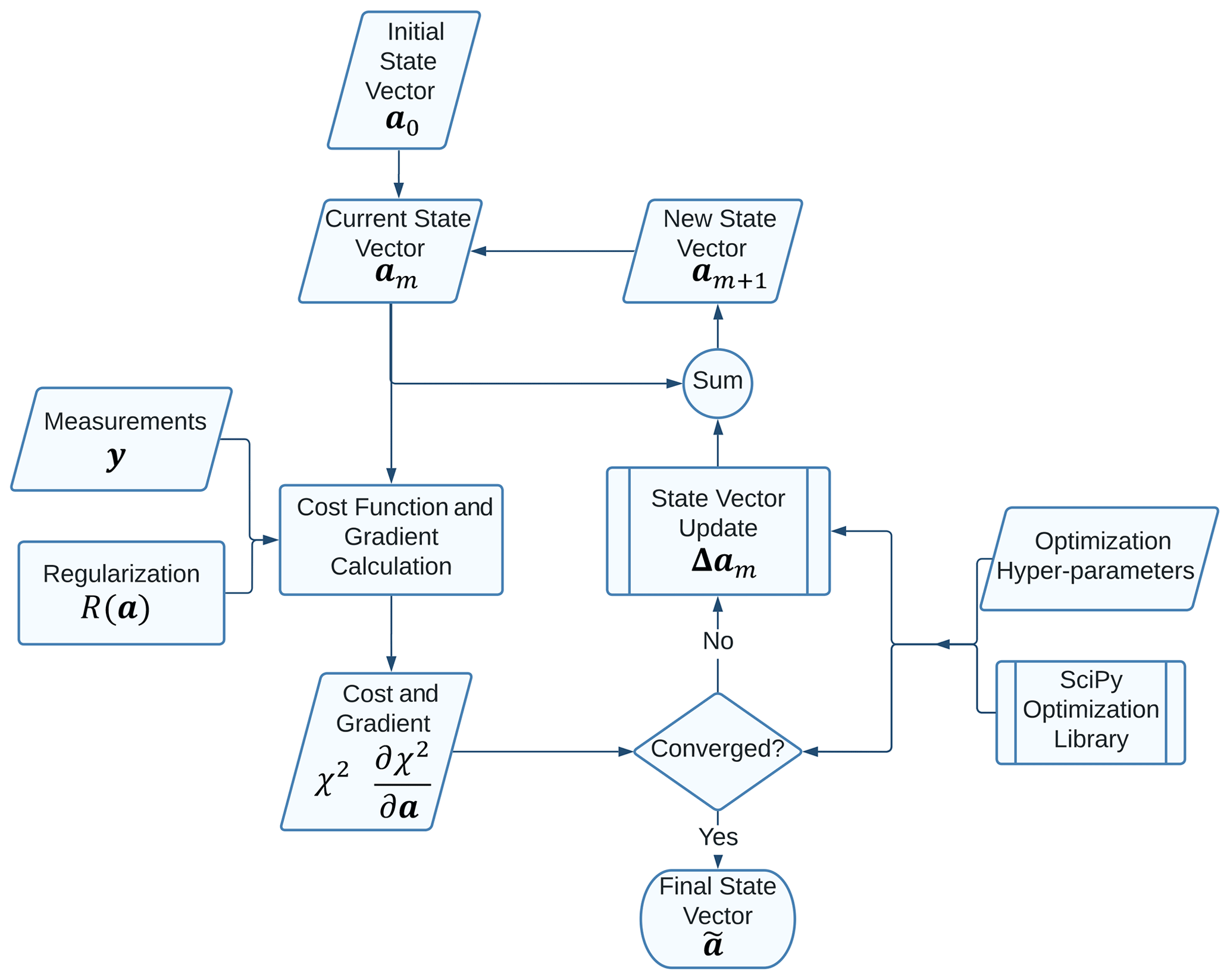
Figure 1A flowchart depicting the overall iterative retrieval methodology of AT3D reproduced from Part 1 (Loveridge et al., 2023a). Section 3.2 and 3.2.1 describe some of the details of how the initial state vector and optimization hyper-parameters are chosen, along with a procedure for synthetically generating some measurements using AT3D.
The solution to the inverse problem can be stated formally as the selection of the state vector that minimizes the cost function subject to box constraints. The box constraints are vectors of lower bounds (l) and upper bounds (u) on each element of the state vector to ensure a valid range for physical variables. For example, liquid water content or volume extinction coefficient should be non-negative. We then have the following:
A local minimization method such as the limited-memory Broyden–Fletcher–Goldfarb–Shannon method for bounded minimization (L-BFGS-B; Byrd et al., 1995) solves Eq. (2) for a locally optimal state vector. Figure 1 presents a flowchart of this process. To use such a method, we need to be able to compute the gradient of the cost function. The gradient of the data fit component of the cost function is given by
where K is the Jacobian matrix containing the partial derivatives of the ith output of the forward model with respect to the jth component of the state vector.
We use the approximate Jacobian matrix calculation, described in Part 1 (Loveridge et al., 2023a), to efficiently compute the approximate gradients of the cost function using the approximate Jacobian :
Our approximate Jacobian matrix is accurate in the single-scattering limit. In this regime, it has a relative root mean square error (RMSE) of 4 % with respect to finite differencing calculations (Loveridge et al., 2023a), which is similar to the accuracy of derivatives calculated using a forward-adjoint formulation (Doicu and Efremenko, 2019). The accuracy of the approximate Jacobian degrades as the medium becomes optically thicker, as the phase function becomes more isotropic, and as the single-scattering albedo and surface albedo increase (Loveridge et al., 2023a). This is due to the larger relative contributions of higher-order scattering to the gradients, which are the contributions which are least accurately modelled in our approximate Jacobian calculation (Loveridge et al., 2023a). When the medium has single-scattering properties representative of cloud droplets at visible wavelengths and the surface is dark (e.g. oceanic), then the relative RMSE in the approximate Jacobian reaches only 12 % for finite clouds, with maximum optical depths of 100 (Loveridge et al., 2023a).
The accuracy of the approximate Jacobian also varies with the angular resolution of the SHDOM solver when phase functions have strong forward-scattering peaks (Loveridge et al., 2023a). This occurs due to the interaction of the angular resolution and the delta-M scaling (Wiscombe, 1977) and truncated multiple-scattering (TMS) approximations (Nakajima and Tanaka, 1988) used in SHDOM. Lower-angular resolution results in more scattering being treated as part of the direct transmission. This results in a decrease in the effective optical thickness of the medium and a corresponding increase in the accuracy of the approximate Jacobian. If the angular resolution is lowered from 16 zenith angle discrete ordinate bins to just 2 zenith angle discrete ordinate bins, then the error in the approximate Jacobian decreases from 12 % to 8 % for the cloud-like media described above.
Errors in the Jacobian calculation lead to errors in the gradient, which limit the convergence of a local optimization method such as the L-BFGS-B method. This is because, in the presence of errors, only small step sizes will accurately predict the change in the cost function to a precision that satisfies the stability criteria in the line search of the optimization procedure (Byrd et al., 1995; Zhu et al., 1997). If errors in the gradient are large, then the optimization may terminate far from an apparent minimum in the cost function, even when the optimization problem is linear (Shi et al., 2021).
There are several factors that complicate this retrieval methodology which uses local optimization. These factors have been discussed in Part 1 and elsewhere in the literature. In the remainder of this section, we briefly summarize these factors which motivate our study and its methodology. In addition to the uncertainties due to our approximate Jacobian calculation, the use of a local optimization method on a non-linear inverse problem also introduces significant uncertainty. As the forward model F(a) is non-linear, multiple local minima in the cost function may exist. This means that the best-fitting state vector estimated from local optimization methods may be strongly sensitive to the choice of initialization and may be far from the globally optimal solution (Rodgers, 2000). Linearized uncertainty estimates may also be inaccurate (Rodgers, 2000; Gao et al., 2022). So far, only local optimization methods have been employed for physics-based cloud tomography (Martin and Hasekamp, 2018; Levis et al., 2020; Doicu et al., 2022b). The proposed BFGS algorithm performs well, compared to other local optimization techniques (Doicu et al., 2022a). Global optimization methods such as ensemble-based particle filters (van Leeuwen et al., 2019) have also been proposed for tomography in other fields (Raveendran et al., 2011). Interestingly, it has been shown that our approximate Jacobian can outperform an unapproximated linearization using forward-adjoint methods, which was suggested to be due to the ability of the approximate Jacobian to escape local minima (Doicu et al., 2022b).
The use of a local optimization method introduces the need to choose a particular initialization for each retrieval. This choice is non-trivial, especially as clouds become optically thick. A poor choice for the spatial distribution of the extinction coefficient, even with a correct average mean free path (or optical diameter), may degrade the retrieval performance. This is because the distribution of an optically thick medium in space is highly non-linear, while adjusting the extinction coefficient within a known volume is weakly non-linear. It has been shown that when the ground truth cloud envelope is used to initialize the retrieval, then the performance of the retrieval improves substantially (Tzabari et al., 2022).
In addition to the complexity of selecting an initial guess appropriate for an optically thick cloud, local optimization is expected to become much more difficult in the regions of state space where clouds are optically thick. This is due to the ill-conditioning of the forward model (Loveridge et al., 2023a). The degree of ill-conditioning of an operator measures its instability to inversion. The condition number of the Jacobian matrix, κ(K), is the upper bound for the relative enhancement of an error in the measurement space when it is propagated by the Jacobian matrix to the state space. We measure the magnitude of errors in a vector using the commonly used Euclidean norm, so then the condition number of a matrix is defined as the ratio of its largest (s1) and smallest (sn) singular values:
In Part 1, we showed that the condition number increases exponentially from well-conditioned κ(K)∼101 to very ill-conditioned κ(K)≫105, as the optical depth of the medium increases from 0.1 to 100.0 for finite clouds (Loveridge et al., 2023a). The largest condition numbers in clouds with maximum optical depths of 100 were associated with maximum and minimum singular values of 0.06 and 2 × 10⁻⁷. The absolute magnitude of these singular values is associated with uncertainty propagation via the Fisher information matrix but are also sensitive to the details of the discretization, such as grid spacing. A condition number that is comparable to or larger than the inverse of the numerical precision of any floating-point numbers is effectively ill-posed, as even rounding errors can propagate to large uncertainties. The exponential behaviour of the condition number is in agreement with theoretical estimates of the stability of the continuous RT problem (Bal and Jollivet, 2008; Chen et al., 2018; Zhao and Zhong, 2019), the perturbative numerical studies of radiative transfer in cloudy atmospheres (Martin and Hasekamp, 2018; Forster et al., 2021), and the field of diffuse optical tomography (DOT; Tian et al., 2010; Niu et al., 2010; Raveendran et al., 2011). This behaviour is due to the smoothing effect of multiple scattering. A smoothing operator is unstable under inversion. This effect of radiative smoothing has been the subject of study in cloudy atmospheres (Marshak et al., 1995; Davis et al., 1997) in the context of optical depth retrieval but is enhanced in a tomographic context due to the finer 3D discretization of the medium (Bal, 2012).
The ill-conditioning in optically thick clouds results in uncertainties that are not evenly distributed throughout the cloud. It has been shown that measurements first lose sensitivity to changes in the cloud in the regions that are optically far from all sensors and also the Sun (Niu et al., 2010; Tian et al., 2010; Forster et al., 2021; Loveridge et al., 2023a). This will result in the largest uncertainties in those regions. In Part 1, we also hypothesized that the large mismatch in sensitivities between these regions and the outer edges and illuminated sides of the optically thick clouds would cause systematic errors in retrievals that use local optimization. There is some indication that this effect occurs in practice, as retrievals performed with an optically thin initialization have underestimations of extinction in the centre of clouds, especially when they are thicker (Levis et al., 2015; Martin and Hasekamp, 2018). One focus of our work is to quantify the extent to which such systematic errors emerge in our retrievals.
In Part 1, we also identified that the magnitude of the loss of sensitivity and ill-conditioning of the forward model in the optically thick limit can be dramatically reduced by lowering the angular resolution of the SHDOM model (Loveridge et al., 2023a). This is again due to the interaction of the delta-M scaling with the angular resolution of the model due to the lowering of the effective optical depth of the radiative transfer. For the same finite clouds described above, the decrease in the magnitude of the condition number of the Jacobian matrix can reach a factor of ∼ 102 when lowering the angular resolution from 16 zenith angle discrete ordinate bins to just 2 zenith angle discrete ordinate bins. This means that a lower-accuracy SHDOM model is less ill-conditioned (due to its lower condition number). The reduction in the condition number is due to more sensitivity to the interior of an optically thick cloud and may be useful for improving retrieval accuracy, despite its larger forward-modelling error. This property is independent of our approximation to the Jacobian matrix (Loveridge et al., 2023a). The reduction in the condition number of the forward model with decreasing angular resolution and the increase in the accuracy of the approximate Jacobian with decreasing angular resolution stem from the same cause but have different effects on a local optimization procedure. Ill-conditioning is the sensitivity of the inversion to errors. The approximation to the Jacobian is a source of error.
The objective of our study is to examine the effectiveness of the local optimization method described in Part 1 to perform cloud tomography. As part of this, we also test the sensitivity of the local optimization to the optical depth of the cloud and to the angular accuracy used in the forward model, SHDOM. Low-accuracy forward models are frequently used to accelerate the iterative solution of optimization problems (Tarvainen et al., 2009; Peherstorfer et al., 2018), and our analysis below provides a first test of whether this approach may also be beneficial in the context of cloud tomography to reduce computational cost.
We perform retrievals on synthetic clouds with stochastically generated 3D fields of volume extinction coefficient. These synthetic clouds are designed to resemble cumuliform clouds and have maximum optical depths that range from 4 to 88. The technical details of the procedure for generating these synthetic measurements for a range of clouds across a range of optical depths are described in Sect. 3.1. We perform retrievals of the 3D volume extinction coefficient using perfect knowledge of the ground-truth atmosphere, surface, and cloud microphysics. This idealized configuration is sufficient to test the efficacy of the approximate Jacobian. We initialize our local optimization by assuming that the cloud is extremely optically thin, which has been exclusively used so far in cloud tomography (Levis et al., 2015, 2017; Martin and Hasekamp, 2018; Levis et al., 2020; Doicu et al., 2022a, b). The precise methodology we use is described in Sect. 3.2 and the associated Appendixes. This configuration acts as a limiting case, as the local optimization will be tested by the high degree of non-linearity of the forward model between its optically thin initialization and the potentially optically thick ground truth. As such, we must stress that our results are likely particular to this choice.
To isolate the fundamental limitations in using the local optimization method with the approximate Jacobian, we perform our analysis in an idealized numerical setting. We perform several inverse crimes in our retrievals by choosing the discretization of the retrieved medium to perfectly match the ground truth and neglecting several important sources of uncertainty, such as the forward model error and instrument calibration uncertainties. The first of these approximations has been routine throughout the numerical studies of cloud tomography (Levis et al., 2015, 2017, 2020; Martin and Hasekamp, 2018; Doicu et al., 2022a, b; Tzabari et al., 2022). Such approximations are also common in the assessment of other algorithms for atmospheric remote sensing, where synthetic measurement data are often generated using the same 1D radiative transfer model used to perform the retrievals (Delanoë and Hogan, 2008; Xu et al., 2022). Such simplifications occur despite the fact that this approximation is known to fundamentally simplify the nature of the inverse problem and thereby cause underestimates of the true retrieval error (Rodgers, 2000; Bal, 2012). Within radiative transfer, a fixed discretization error also implies a homogeneity assumption below a scale that is likely unrealistic for real clouds, which can cause biases in the resulting modelling of the radiative transfer (Marshak et al., 1998; Davis and Marshak, 2004; Bitterli et al., 2018).
Measurement noise tends to decrease from 1 % to just 0.1 % for cloudy signals as the measured radiance increases (Bruegge et al., 2002). Measurement noise has typically been included in cloud tomography studies so far (Levis et al., 2015, 2020; Tzabari et al., 2022), although, in some cases, this source of uncertainty has also been neglected (Doicu et al., 2022a, b). The magnitude of this noise is much smaller than forward-modelling errors that can range up to several percent in a root mean square sense (Evans, 1998; Cahalan et al., 2005; Pincus and Evans, 2009). These uncertainties have been neglected so far, with the exception of the study of Martin et al. (2018), which used an inflated measurement error of 2 % as a proxy for the modelling error.
In our study, we perform sets of retrievals that use both perfect, noise-free measurements and also those that include idealized measurement noise to ensure that our conclusions about the fidelity of the retrieval are robust with respect to the noise-free assumption. Even with this analysis, we must emphasize that our retrievals are highly simplified, and so the errors in our retrievals should only be interpreted as a tentative lower bound for errors that might occur for retrievals applied to real data.
We analyse seven types of retrieval. First, we have perfect model retrievals, in which we use exactly the same forward model configuration and discretization of the medium during the retrieval that was used to generate the synthetic measurements. This type of retrieval uses noise-free measurements and the naïve, optically thin initialization which we describe in Sect. 3.2. These retrievals are referred to as “Default” retrievals. Retrieval accuracy in this configuration is limited only by the non-linearity of the inverse problem and the errors in the approximate Jacobian, both of which are deterministic.
Second, we perform retrievals that are the same as the Default, except that they use a low angular accuracy forward model. These are referred to as “Low” retrievals. This retrieval acts as a test of how much the retrieval changes when using an approximate forward model that is less ill-conditioned (has a lower condition number) and has a more accurate gradient calculation. The differences between the Default and Low retrievals may occur as a result of changes in the optimization trajectory either close to or far from the local minimum in the cost function. To distinguish between these two types of effects, we perform a third set of retrievals. These retrievals use the same configuration as the Low retrieval, except that they are initialized at the ground truth (GT) and are referred to as “Low-GT”. The drift in the state vector away from the ground truth during the optimization acts as a measure of the error induced by using a low angular accuracy model in the retrieval in the vicinity of the global minimum.
We also include two sets of “Restarted” retrievals. The restarted retrievals make use of the results of the Low retrievals to initialize retrievals that use the perfect forward model from the Default retrievals. These restarted retrievals are referred to as the “20th Low iteration Restart” and “Final Low iteration Restart”, based on the iteration of the Low retrievals from which the state vector is taken to initialize the new restarted retrieval. These retrievals test our ability to mitigate any errors forming in the Low retrievals by using the perfect forward model.
Additionally, we perform two sets of experiments to ensure the robustness of our conclusions to the presence of noise or other small inconsistencies between the synthetic measurements and the forward model. First, we perform retrievals initialized at the ground truth that make use of noisy measurements and the perfect model from the Default retrievals. These are referred to as “Noisy-GroundTruth” retrievals. Second, we repeat the Default and Low experiments using noisy observations and use the differences to assess the robustness of our results. These retrievals are referred to as “Default-Noisy” and “Low-Noisy”.
3.1 Synthetic measurement generation
We generate the synthetic measurements entirely using the cloud fields, RT, and instrument modelling implemented in AT3D. The only scattering particle species under consideration in each retrieval is an isolated water cloud (i.e. no molecular scattering or absorption). We assume that the cloud scattering is conservative (ω=1) and that the phase function is from Mie calculations of a gamma distribution of spherical water droplets with an effective radius of 10 µm and effective variance of 0.1 at a wavelength of 0.86 µm. Vacuum horizontal boundary conditions are used, and the bottom surface is prescribed to be black. There is only a solar source and no thermal emission.
The clouds used in this study are stochastically generated rather than generated by large-eddy simulations (LESs), as is common in many retrieval validation studies (Marshak et al., 2006; Kato and Marshak, 2009; Ewald et al., 2019). This choice is made primarily for control over the media. Realistic covariances between microphysical parameters, which is one of the primary benefits of LESs (Miller et al., 2018), are not required for these retrievals, as only a single spatially variable parameter is being retrieved (i.e. volume extinction coefficient). With stochastic generation, we can control the spatial variability at all scales and produce difficult, non-smooth extinction fields at scales of tens of metres with great ease that would otherwise require undue computational expense with LESs.
The stochastic cloud generator used to generate the extinction fields is included with AT3D. It is based on similar statistical principles utilized elsewhere for synthetic cloud generation (Cahalan et al., 1994; Iwabuchi and Hayasaka, 2002; Prigarin and Marshak, 2009). Such principles include the fact that liquid water content tends to have a positively skewed distribution (e.g. lognormal) and that the power spectrum of its variability tends to follow a power law (Davis et al., 1999). The unique aspect of this generator is that it is targeted at generating isolated clouds rather than large fields with periodic boundaries. The algorithm proceeds as follows:
-
Two fields of white Gaussian noise with zero mean and unit variance are generated with skewness < 0.1 and kurtosis < 0.5. One will form the binary volumetric cloud mask, and the other will form the 3D field (e.g. extinction or liquid water content). This separation is done so that the smoothness of the cloud boundary can be controlled independently. It also introduces additional small-scale variability to the field by allowing large discontinuities between in-cloud and cloud-free field values.
-
The fast Fourier transform (FFT) of each field is obtained and then scaled so that the power spectrum follows a power law with a specified exponent. We used an exponent of , which is supported by various in situ measurements of horizontal variability in the cloud liquid water content (Davis et al., 1996, 1999) and nadir radiance measurements (Lovejoy et al., 1993; Lewis et al., 2004). The resulting fields are then inverse Fourier transformed back into the physical space.
-
The two fields are exponentiated to obtain positively skewed (e.g. lognormal) statistics typical of clouds.
-
The cloud mask field X is scaled by an anisotropic Butterworth filter in physical space to enforce small values near the boundaries of the domain. This counteracts the periodic nature of the FFT process used to generate the noise and allows the generation of isolated clouds that have a blob-type shape that tends to maximize in the centre of the domain. Note that there is no specific requirement for a single contiguous cloud mass, though this filter does encourage it. The filtered cloud mask field is expressed as
where R is the horizontal distance from the centre of the domain, and z′ is the vertical distance from the centre of the domain. The two scale parameters are set to α=0.2 and β=0.2.
-
The cloud mask field is then thresholded to obtain a user-specified volume cloud fraction of 10 %.
-
The points in the second field are set to zero, where the cloud mask field is designated as clear.
-
The second field is scaled so that its mean and variance have a user-specified vertical profile over the cloudy points and so that it forms the 3D field of, for example, the volume extinction coefficient.
We use 10 different random seeds and 4 different vertical profiles of horizontally averaged extinction, thus generating 40 cloud models in 4 categories of maximum optical depth (Loveridge, 2023). Each of the four profiles prescribes a linear increase in the mean extinction with height. Note that this is a more rapid increase in the extinction with height than predicted by the adiabatic theory, namely that the extinction increases as , with h being the height above cloud base. At each level, the deviations from the mean are scaled so that the standard deviation is chosen to be 40 % of the mean at that level. Each cloud is generated on a grid of (25 × 25 × 25) grid points with 40 m resolution, forming a domain of (1 km)3. We name the four categories of cloud models Thin, Medium, Thick, and Very Thick. They have maximum vertical optical depths of 4, 17.5, 44, and 88, respectively.
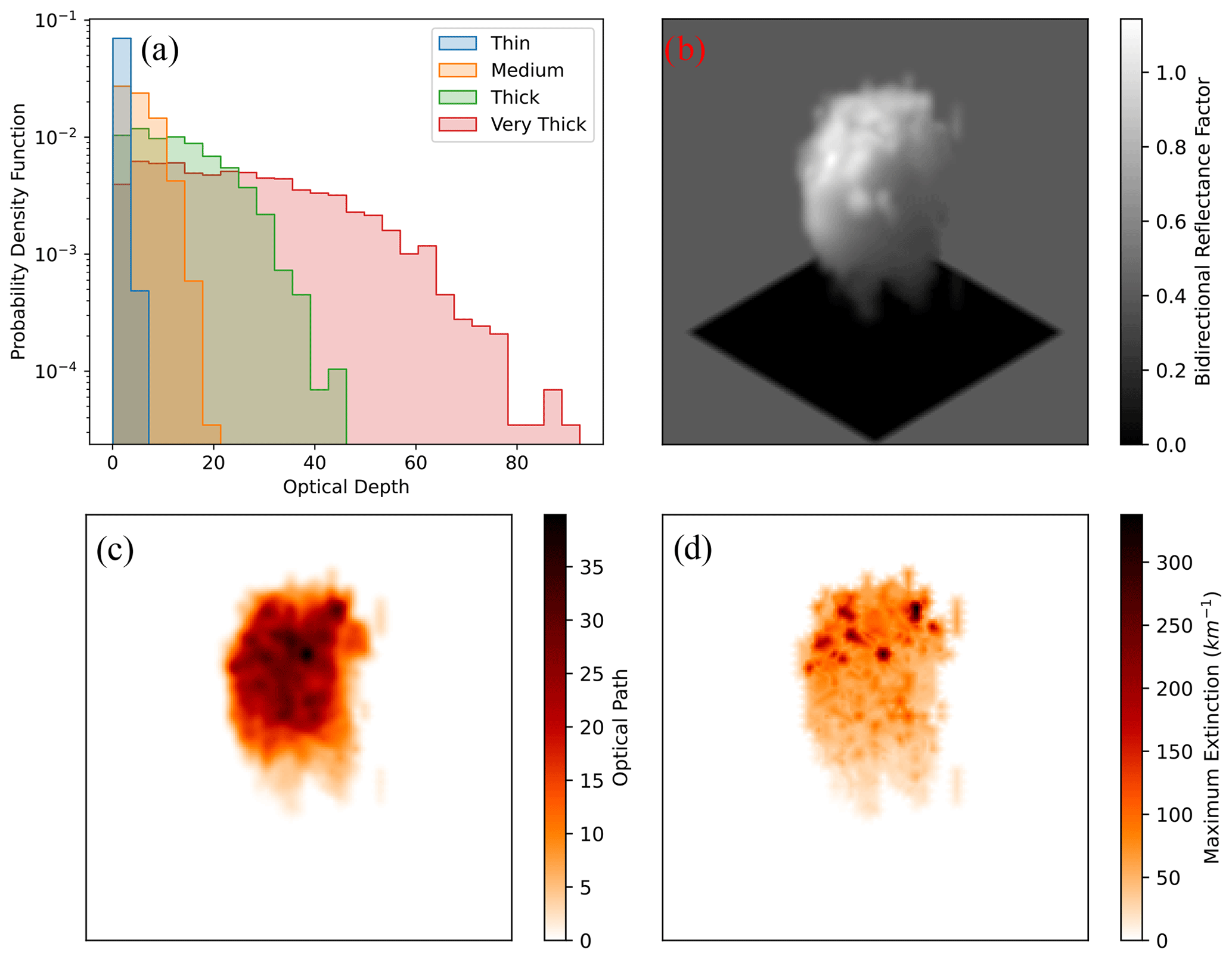
Figure 2(a) The probability density functions of cloud optical depth for stochastically generated clouds in the Thin, Medium, Thick and Very Thick categories. Each category contains 10 clouds. (b) An image of cloud realization no. 4 in the Thick category calculated using SHDOM. The set-up is identical to the other simulations (the solar zenith angle or SZA is 60∘), apart from the fact that the (1 km)3 domain is surrounded by a Lambertian surface with an albedo of 0.4 to give a sense of perspective, which does affect the radiance calculation. The image is captured using a synthetic sensor, following a perspective projection that has a 2.5∘ field of view with 200 by 200 pixels and is viewing the centre of the domain from a position of x = y = z = 20 km (central viewing zenith angle of 55∘ and relative azimuthal angle of 45∘). (c) The optical path along each pixel's line of sight is under the same projection as in panel (b). The maximum value of the volume extinction coefficient along the line of sight under the same projection is as in panel (b). Two cross sections through this cloud are also shown in Fig. 6.
Figure 2a shows the optical depth distributions of each of the four categories of clouds (left panel). For one example cloud realization, we also show an image of the cloud (Fig. 2b) and the optical path and maximum volume extinction coefficient along the same lines of sight. These figures show the high degree of variability in the extinction fields (Fig. 2d) and the decorrelation of the optical path from the radiance field (Fig. 2b vs. Fig. 2c) due to the non-local transport process. Note that the decoupling of the extinction and cloud mask fields in the stochastic generator can produce true voids within the cloud. The cross sections of the extinction field (e.g. Fig. 4) of a cloud reveal that the extinction fields can be much more variable than might be expected from an LES-generated cloud at small scales (Eytan et al., 2022). This is a carefully considered choice, as we want to test the limits of the retrieval on non-smooth media to detect, for example, a smoothing bias.
The synthetic measurements used in this study are chosen to mimic an airborne multi-angle imager such as AirMSPI (Airborne Multiangle SpectroPolarimetric Imager) operating in a step-and-stare mode (Diner et al., 2013), with the exception that all measurements are acquired simultaneously in this synthetic scenario. This is a similar configuration to that which can be achieved with the upcoming CloudCT mission (Schilling et al., 2019), which will utilize a constellation of small satellites to obtain simultaneous multi-angle imagery. Here, we model the imaging geometry as orthographic projections of the domain with a fixed azimuthal orientation at right angles with the principal plane of the Sun, i.e. relative azimuth of 90 and −90∘. The use of an orthographic projection is a highly approximate camera model but is suitable for approximating a small domain near the centre of the swath of a push broom sensor. In addition to a nadir view, there are images with viewing zenith angles of [75.0, 60.0, 45.6, 26.1∘] on either side of the principal plane for a total of nine views. This is the most used viewing angle configuration that has been used to test a 3D tomographic retrieval and has demonstrated success in several cases (Levis et al., 2015, 2017, 2020; Doicu et al., 2022a, b), so it forms a useful reference configuration on which to test the variation in the retrieval accuracy with optical depth to help connect with other published results.
The solar zenith angle is chosen as 60∘. This differs from other studies which have typically used a smaller solar zenith angle (Levis et al., 2015, 2017, 2020; Doicu et al., 2022a, b). We chose the larger value so that we can more easily discern the effects of any error features that are oriented with respect to the Sun in our results, as was hypothesized in Part 1. This choice also puts the observations close to the scattering angles of maximum error in the approximate Jacobian (see Part 1, where we quantified the scattering angle dependence of the error in the approximate Jacobian calculation); hence, a worst-case scenario is found.
The measurement resolution is set to 35 m. The AT3D models the pixel-level radiance measurements as a weighted sum of the idealized singular samplings of the radiance field within a field of view. For simplicity, we choose a single quadrature point at each pixel centre to model the pixel radiance in the simulation of the synthetic measurements. Choosing the measurement resolution (35 m) to be slightly smaller than the grid resolution (40 m) ensures that all of the grid points are evenly sampled by the measurements, even with the single quadrature point per pixel. This ensures the basic numerical stability of the retrieval, by ensuring that it is over-constrained and that the use of regularization is not a strict requirement. The SHDOM solver uses 16 zenith discrete ordinate bins, 32 azimuthal discrete ordinate bins, a splitting accuracy of 0.03, and a solution accuracy of 10−4, with no truncation of the spherical harmonics. The scalar approximation (no polarization) to the RTE is utilized.
In the Default-Noisy, Low-Noisy, and Noisy-GroundTruth experiments, noise is included in the measurements. The noise model used for this procedure is described in Appendix A. For each of the 40 sets of measurements, a fixed set of noise perturbations is generated through the selection of a random seed. These same noisy measurements are utilized in all retrieval experiments that make use of noisy measurements.
3.2 Inverse problem set-up
The same forward model described above is used in most of the experiments, except our Low retrievals. In these retrievals, the angular accuracy in the SHDOM solver is reduced to just two zenith discrete ordinate bins and four azimuthal discrete ordinate bins. All other numerical parameters are the same.
The state vector is chosen as a subset of the grid points that are potentially cloud-containing points, according to a space-carving procedure (Kutulakos and Seitz, 1999) that uses 2D binary cloud masks from each of the multi-angle images (Lee et al., 2018). This procedure follows Levis et al. (2020). The space-carving procedure rules out clouds along the line of sight of all pixels that are classified as clear. The details of the space-carving algorithm and its performance are presented in Appendix B. The cloud masking of the multi-angle images is trivial, due to the absence of a scattering surface or atmosphere (Yang and Di Girolamo, 2008). For the retrievals that use a naïve, optically thin initialization, the elements of the state vector are set as 0.01 km−1. Additional descriptions of the hyper-parameters of the optimization using the L-BFGS-B algorithm including the stopping conditions are in Appendix C.
We now present the results of the retrievals and discuss the accuracy of the retrieved extinction fields and their robustness to noise (Sect. 4.1), the accuracy of inferred optical depths (Sect. 4.2), and the computational expense (Sect. 4.3). To quantify the performance of the extinction retrieval, we use the relative bias and relative RMSE of the volume extinction field, which is expressed, respectively, as
where and .
In the above equations, σ is the volume extinction coefficient. We also calculate the relative bias in the coefficient of variation (standard deviation divided by mean) of the retrieved extinction field to quantify the heterogeneity of the retrieved cloud. We also apply these three metrics to the assessment of other variables such as optical depth. We refer to the error metrics in units of percent (%) within the text for clarity. Simple differences in the error metrics between two retrievals are also reported in percent. Error metrics are defined by comparison with respect to the ground truth, unless otherwise specified.
The error metrics are evaluated over all grid points in the (1 km)3 domain, and not the elements of the state vector, which only includes the grid points specified as cloudy by the space-carving algorithm. In general, the fidelity of a 3D retrieval should be evaluated over the physical fields in the domain rather than a metric on the state vector space. This facilitates comparison with other retrieval methods, which may not use the same spatial basis. The relative bias and relative RMSE of the extinction field are invariant to the inclusion of points for which there are no errors. The space-carving approach employed here has no false negatives, and as such, the values are the same as if the error metric were applied to the state vector.
4.1 Extinction retrieval
Let us first consider the robustness of the results to noise before interpreting them in detail. The accuracy of the Default and Low retrievals using noise-free measurements is shown in Table 1. The ensemble-averaged error metrics with respect to the ground truth differ by less than 1 % between the noise-free retrievals (Default and Low) and the noisy retrievals (Default-Noisy and Low-Noisy). For this reason, we do not report the retrieval accuracies for the Default-Noisy and Low-Noisy retrievals. Instead, we report their differences with respect to the noise-free retrievals (Table 2). Additionally, we found that the retrieval errors in the Noisy-GroundTruth retrievals were less than 0.01 % for all realizations in all cloud categories, so we do not report further details of the results of those retrievals. Immediately, we can see that the ensemble-averaged results are robust to the inclusion or exclusion of noise.
Table 1Extinction errors for the different retrieved clouds in each category. The means of the error metrics are shown across the 10 clouds in each category, with the standard deviation across the 10 clouds in parentheses. See the text for details of the error metrics.
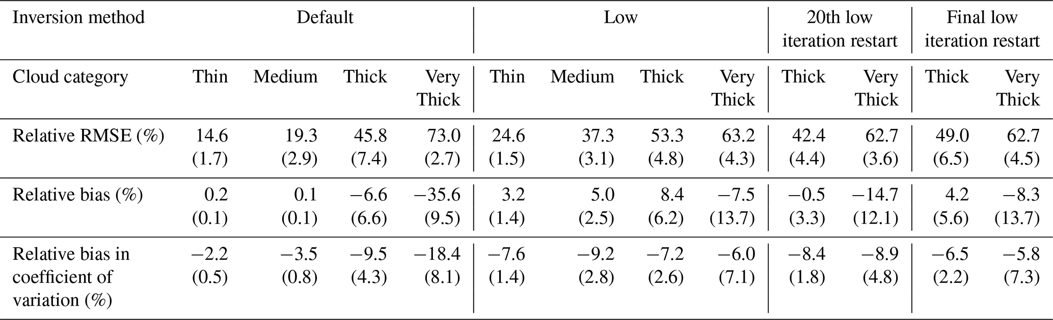
Table 2Differences between the extinction fields from noisy and noise-free retrievals. The means of error metrics are shown across the 10 clouds in each category, with the minimum and maximum across the 10 clouds in parentheses. See the text for details of the error metrics.
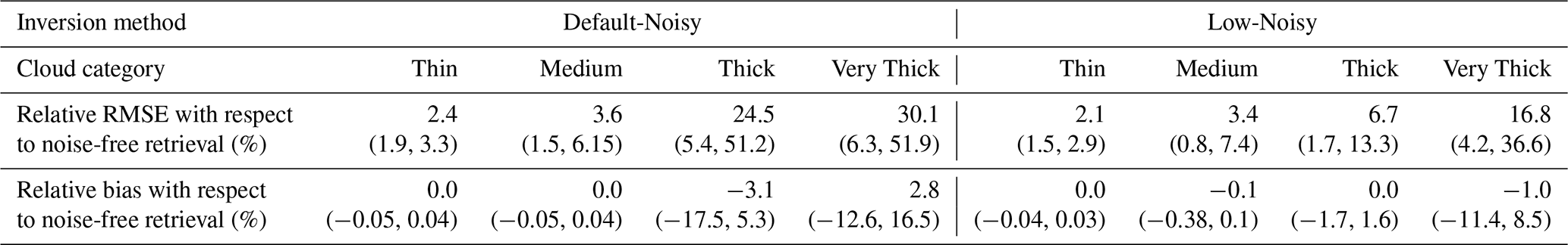
The differences between the noisy and noise-free retrievals increase with optical depth (Table 2) and can include large systematic differences between retrievals for particular realizations in the Thick and Very Thick cloud categories. This latter feature can be seen in the large ranges of the error metrics in Table 2 for the Very Thick cloud category. The large deviations between noise-free and noisy retrievals indicates large uncertainties in these retrievals. The differences in between the Default or Low retrievals and their corresponding noisy variants (Table 2) are much larger than the retrieval errors in the Noisy-GroundTruth retrievals (which are negligible). This large discrepancy indicates that the issues of non-linearity and errors in the local optimization will confound uncertainty quantification, as the ensemble-based uncertainty estimates will differ, depending on the choice of initialization. We revisit the implications of this point in Sect. 5. We focus the rest of our analysis on explaining the variability in the retrieval accuracy for the noise-free retrievals.
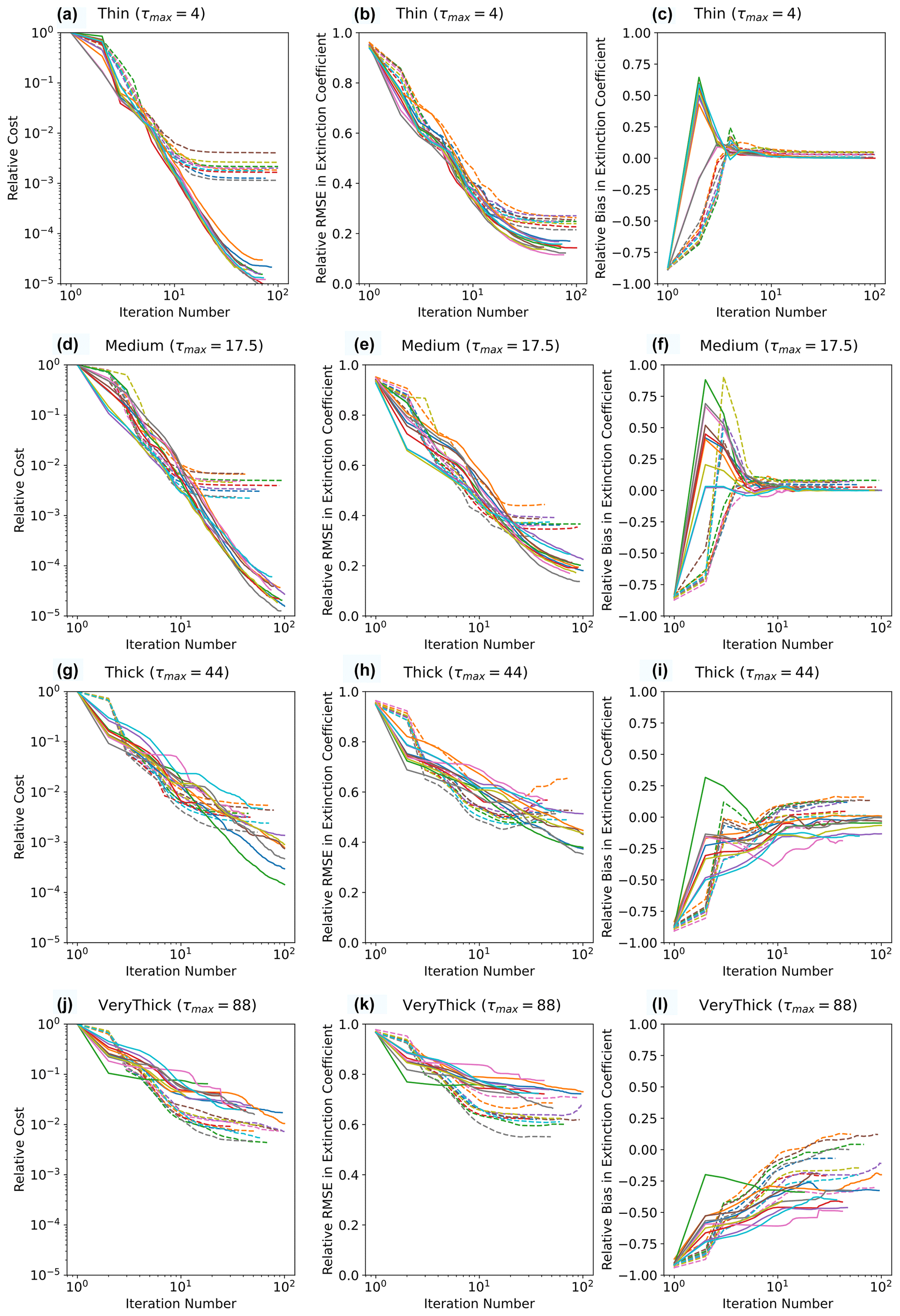
Figure 3Retrieval performance for the Default (solid lines) and Low (dashed lines) retrievals as a function of iteration number for clouds in the Thin (a–c), Medium (d–f), Thick (g–i), and Very Thick (j–l) categories. Each coloured curve corresponds to a different cloud realization. The first column (a, d, g, j) shows the cost function normalized by its initial value. The second column (b, e, h, k) shows the relative RMSE (Eq. 6) in the retrieved volume extinction coefficients. The third column (c, f, i, l) shows the relative bias (Eq. 7) in the retrieved volume extinction coefficient. See the main text for details of the error metrics. Note the logarithmic scale of the iteration number, given that computational expense is linear in iteration number.
The Default retrievals for the Thin and Medium cloud categories are uniformly accurate, with negligible bias and small relative RMSEs (Table 1). The Low retrievals have lower accuracies than the Default retrievals for these two categories, due to their large forward-modelling error. The cost function of the Low retrievals for the Thin and Medium cloud categories (Fig. 3) begins to decrease very slowly with the iteration number after only around 20 iterations and asymptotes to a larger value than for the Default retrievals. The local optimization can proceed for ∼ 100 iterations for the Default retrievals in the Thin and Medium cloud categories. However, the results for the Low retrievals indicate that retrievals may converge within far fewer iterations for these clouds in the presence of modelling and instrumental errors. Given the good performance of the Default retrievals, we do not consider any Restarted retrievals for the Thin and Medium cloud retrievals. The worse performance of the Low retrieval indicates that there is no benefit from the better conditioning and more accurate Jacobian approximation for these clouds.
The accuracy of the retrievals systematically degrades with increasing optical depth. The rate of reduction in the cost function with iteration number decreases as the optical thickness of the clouds increases (Fig. 3), which can be seen by comparing the behaviour of the Medium, Thick, and Very Thick cloud categories. The relative RMSE systematically increases with optical depth (Table 1) for both the Default and Low retrievals, and a large bias of −36 % develops in the Default retrievals in the Very Thick category. This bias is dramatically reduced to just −7 % in the corresponding Low retrievals. The convergence behaviour of the Low retrieval for the Very Thick clouds (Fig. 3l) shows that the Low retrieval more rapidly increases the mean extinction with iterations, particularly beyond 10 iterations, where the cloud has become optically thick. The final cost functions obtained by the Low retrievals are much lower than the Default retrieval. This is associated with a lower relative RMSE in the final modelled radiance fields of just 9 % when compared to 16 % for the Default retrieval. The differences between the Default and Low retrievals for the Thick clouds are milder but are still significant, with a lower relative RMSE and slight improvements in the bias.
The dramatic improvement in the reported accuracies of the Low retrieval for the clouds in the Very Thick category indicates that there is a substantial sensitivity of the retrieval to the choice of angular resolution in the forward model. The apparent benefit of using the Low-accuracy retrieval is carried through into both types of Restarted retrievals. Using the high-accuracy forward model in the Restarted retrieval does little to improve the retrieval accuracy beyond that of the Low retrieval used to initialize it (Table 1). This indicates that the local optimization algorithm is unable to further reduce the residuals, despite the use of a more accurate forward model.
Table 3Extinction errors for the Low-GT retrievals. The means of the error metrics are shown across the 10 clouds in each category, with the standard deviation across the 10 clouds in parentheses. See the text for details of the error metrics.
The faster convergence of the mean of the Low retrieval, when compared to the Default retrieval in the Very Thick category (Fig. 3l), suggests that it is the better conditioning of the forward model that drives the improvement in the convergence. However, the improvement in the retrieval accuracy may be due to compensating biases in the approximate forward model. To help us distinguish between these effects, we make use of the results of the Low-GT retrievals (Table 3). These retrievals are initialized with the ground truth cloud but use the Low-accuracy forward model. The resulting retrieval errors are therefore a local estimate of the error in the retrieved state due to forward-modelling errors in the vicinity of the ground truth. The retrieval errors for the Low-GT Thin and Medium clouds are similar to those of the standard Low retrieval. This further solidifies the good behaviour of the retrievals in these cloud categories.
The relative bias of the Low-GT retrieval for the Thick cloud category is 10.2 % in the ensemble average (Table 3). This shows that much of the difference between the relative bias in the Default and Low retrievals can be explained by the forward model error. In particular, the Low-accuracy model produces smaller radiances for a given optical thickness of the cloud, so the cloud must be biased high in optical thickness to minimize a misfit against the measured radiances. The retrieval bias of the Low-GT retrieval in the Very Thick clouds is only 6.2 %. This is much smaller than the difference in relative bias between the Default retrieval and the Low retrieval. As such, the forward model error in the vicinity of the solution cannot entirely explain the discrepancy between the two techniques. Part of this discrepancy is caused by the fact that the Default retrieval does not converge to the vicinity of the truth in terms of average extinction, and so the forward model error at the ground truth is not representative. However, the bias difference is still much larger than the 10.2 % bias that occurs for the Thick category. The other component of the difference between the Default and Low retrievals is because the trajectory of the local optimization from the optically thin initialization to the final retrieved state is very different.
To better understand the differences in the optimization trajectories between retrievals that use different forward models, let us examine the spatial structure of the extinction errors. Understanding the character of these errors is important for us to understand how to mitigate these errors, particularly in the optically thick limit, and for us to understand whether a low-accuracy, less ill-conditioned forward model may be a part of a mitigation strategy. In doing so, we explain how such a biased extinction field can be retrieved that still provides a relatively small misfit against the radiance measurements in the optically thick limit.
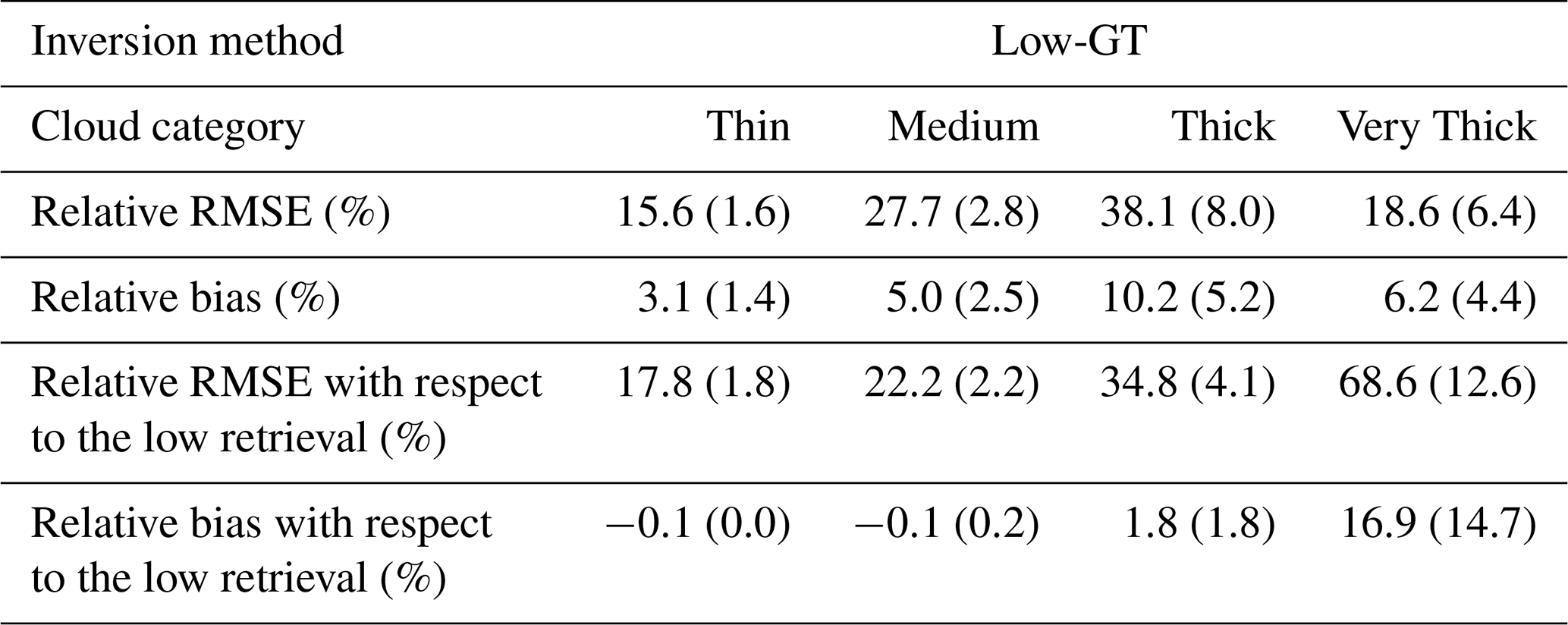
As a starting point in our analysis of the spatial structure of the retrieval errors, let us note that all retrievals have underestimated the variability in the retrieved extinction field, especially at larger optical depths in the Default retrieval. This is demonstrated through the errors in the coefficient of variation in the extinction field (Table 1). We further examine the spatial dependence of this error by examining cross sections of the retrieved extinction field. In Figs. 4 to 7, we show cross sections of the volume extinction coefficient for cloud realization no. 4 of the stochastic clouds, as it is representative and provides all of the key points from the other realizations when visualizing the spatial structure of the errors. We show just the Default and Low retrievals, as the Restarted retrievals are qualitatively similar to the Low retrievals. Cross sections of the extinction field are shown for the slices through the centre of the domain aligned along the azimuthal directions of the sensors and the Sun. We refer to these slices as the measurement plane and solar plane, respectively.
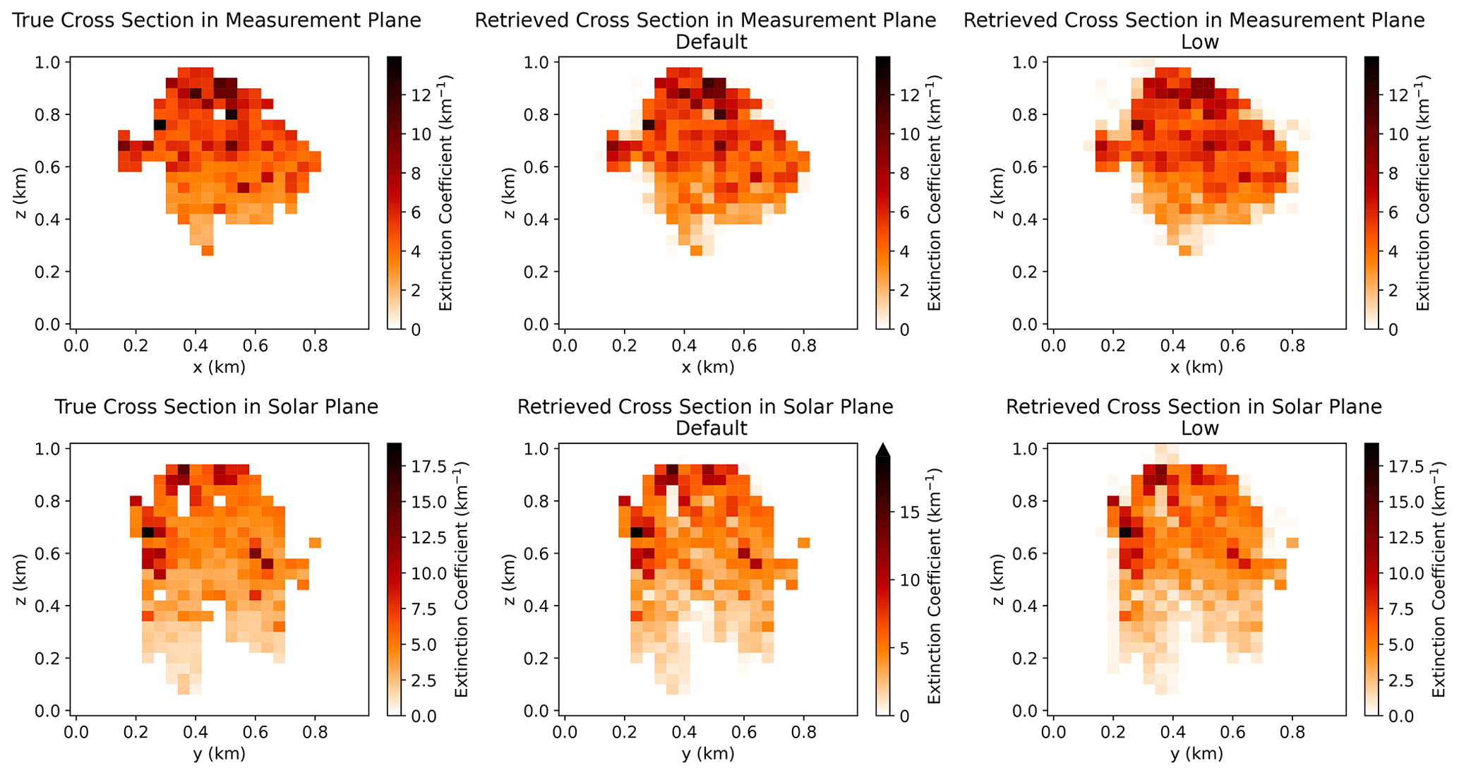
Figure 4Vertical cross sections of the true extinction field (a, d), Default retrieved extinction field (b, e), and the Low retrieved extinction field (c–f) for cloud no. 4 in the Thin category. Cross sections are in the y = 0.48 km plane (a–c) and the x = 0.48 km plane (d–f). The Sun points in the positive y direction, while the viewing directions are aligned along the x axis.
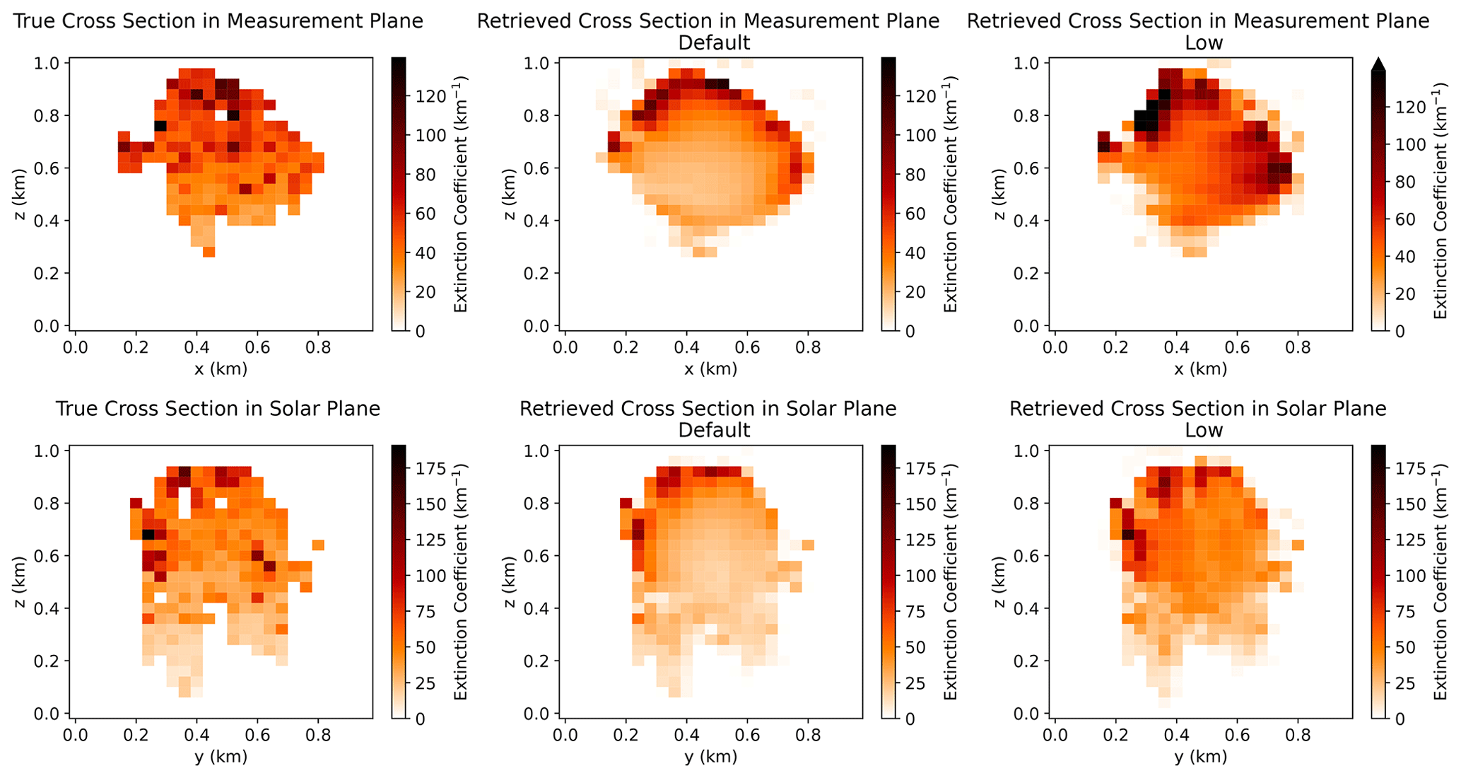
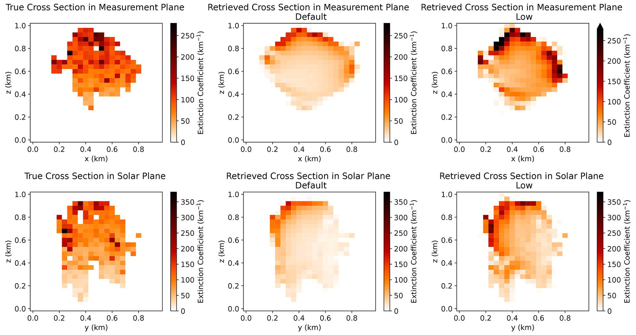
The high-frequency details of the extinction field are retrieved almost perfectly for the Thin (Fig. 4) and Medium (Fig. 5) clouds, with only mild errors apparent in the measurement plane of the Medium cloud. On the other hand, for the Thick (Fig. 6) and Very Thick (Fig. 7) clouds, the extinction field is extremely smooth. There is a gradient of extinction in the solar plane from the illuminated side (left) to the shaded side (right) of the retrievals of the Thick and Very Thick clouds. Fine details of the extinction field are retrieved on the illuminated side but not on the shadowed side. Additionally, the largest values of the retrieved extinction tend to be at the edge of the cloudy volume (as defined by space carving) in the measurement plane, with the smallest values in the centre. This feature is most apparent in the Default retrievals.
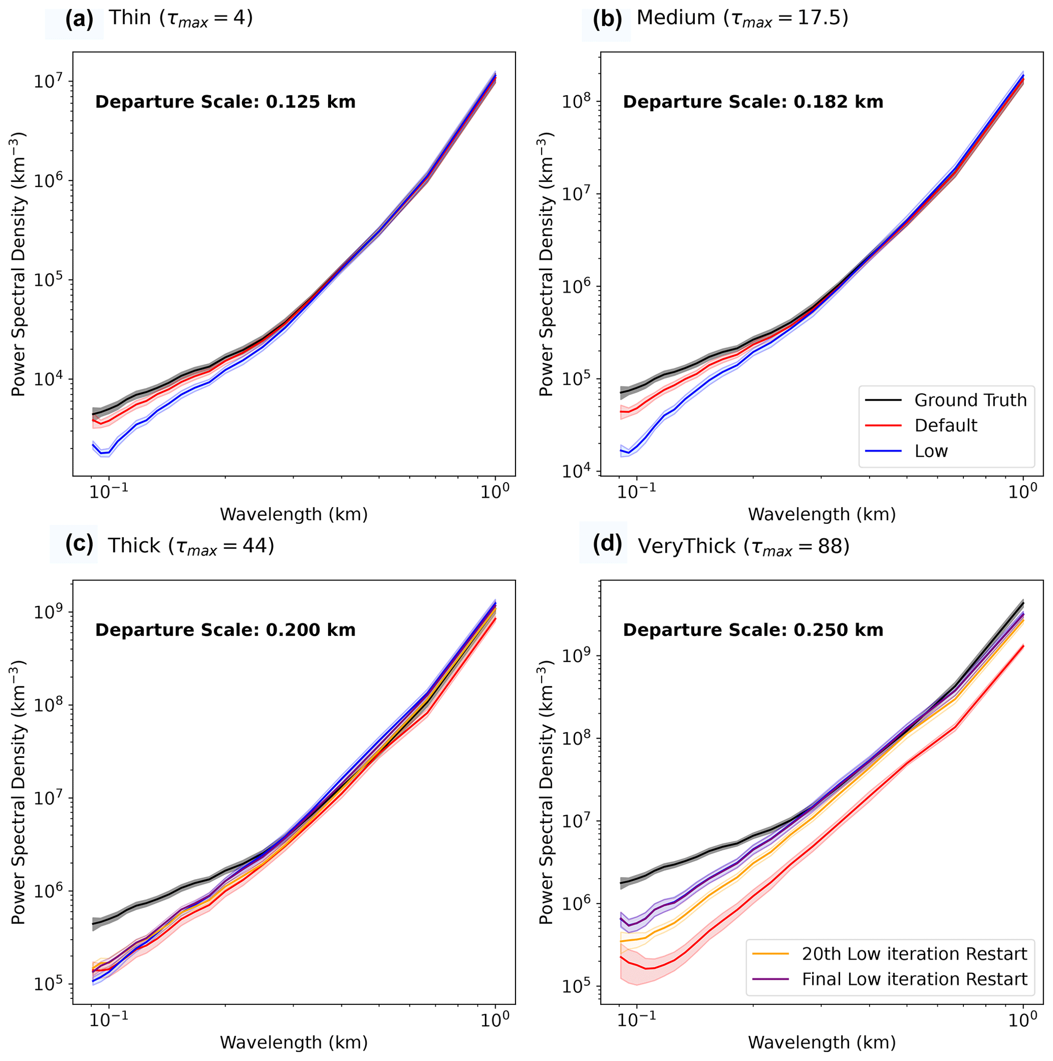
Figure 8The ensemble-averaged and isotropically averaged power spectral density of the volume extinction coefficient for the Thin (a), Medium (b), Thick (c), and Very Thick (d) cloud categories. Solid lines are the ensemble averages, and the shading indicates ± 1 standard error in the mean. The spatial scales of the first departure from the ground truth spectrum by the best-performing retrievals for each cloud category are marked in the top left corners of each figure. Note that, in panel (d), the Low and Restarted final curves are indistinguishable.
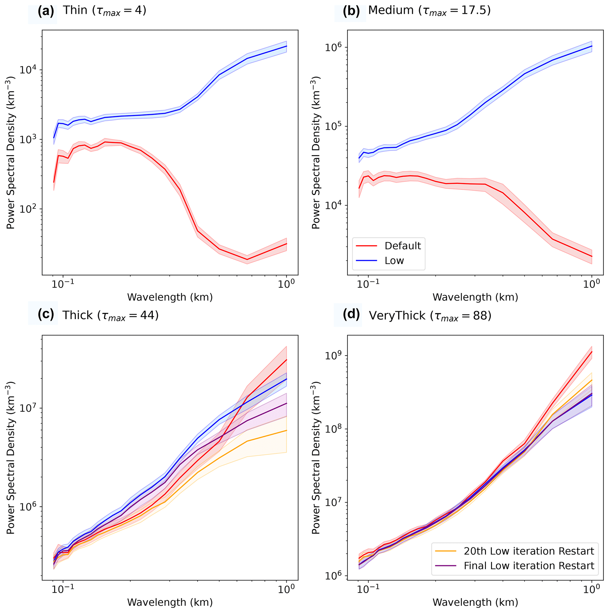
Figure 9The ensemble-averaged and isotropically averaged power spectral density of the errors in the volume extinction coefficient for different retrievals of the clouds in the Thin (a), Medium (b), Thick (c), and Very Thick (d) categories. Solid lines are the ensemble averages, and the shading indicates ± 1 standard error in the mean. Note that, in panel (d), the Low and Restarted final curves are indistinguishable.
To examine the scale-by-scale apportionment of the error across the whole ensemble of retrievals, we use Fourier analysis. Fourier analysis is a global analysis, so it cannot identify, for example, a lower error in small-scale features on the illuminated side of the cloud. To compress the information, we show just the isotropic, ensemble-averaged power spectral density of the retrieved extinction fields (Fig. 8) and their errors (Fig. 9). The retrievals tend to be significantly smoother than the ground truth at small scales. The scale below which the retrieval has less variability when the truth increases from 125 to 250 m, as the clouds become optically thicker. Note that the default retrieval for the Very Thick clouds tends to underestimate variability at all scales; this is an error that is reduced in the Low and Restarted retrievals and is consistent with the reduction in the underestimation of variability (Table 1). Note that the reproduction of approximately correct power spectra at large scales does not necessarily indicate that the retrievals are error-free at these scales, since the phasing of the spatial modes can still disagree and lead to errors proportional to the amplitude of the mode.
The errors in the Default retrievals of the extinction for the Thin and Medium cloud categories are actually band-limited to small scales (Fig. 9). Errors tend to occur primarily at larger scales for the other retrievals, especially in the Thick and Very Thick categories. This indicates that even large-scale features are not accurately retrieved in the Thick and Very Thick clouds, in general, which is in concurrence with Figs. 6 and 7. The primary benefits of the Low and Restarted retrievals in terms of overall reduction in the RMSE are felt at the largest spatial scales (Fig. 9).
The spatial structure of the retrieval error for the Default and Low retrievals of the clouds in the Thick and Very Thick categories for the naïve, optically thin initialization give us some important insight into some of the issues that arise in retrievals of optically thick clouds. The details of the spatial structure of the error in our retrievals are unique to our choice of initialization. In the discussion below, we distinguish between the explanation of our retrieval errors and the hypotheses that we make about the general behaviour of the local optimization in the optically thick limit.
For our particular retrievals, the optically thick cloud state is approached from an optically thin cloud state. During the early iterations, the residuals are highly smooth, as we initialize with an extremely optically thin cloud. As such, the optimization updates the cloud by reducing the bias in the radiances and fills the cloud with a relatively smooth extinction field. As the bias reduces, the cloud becomes optically thick, and now the optimal strategy to reduce the cost function is to further increase the extinction on the illuminated side of the cloud and at the cloud edge in the plane of the measurements. This patterning is because the magnitudes of the Jacobian elements are largest in these positions, as described in detail in Part 1. With the bias in the cost function reduced, the radiance residuals can be multi-signed and mapped more strongly to smaller-scale spatial features in the extinction field. However, the cloud is now optically thick, and this mapping is highly ill-conditioned. So, it is difficult, from a linearized perspective, to redistribute extinction between the outer and inner portions of the cloud while avoiding an increase in the cost function. Tiny step sizes must be utilized to avoid instability, but even these are corrupted by the increasing error in the approximate linearization. Eventually, the cost function reductions are so small that the stopping condition of the optimization is achieved. This results in the presence of gradients in cloud extinction from the illuminated to the shadowed side and from the cloud edge to the cloud core in the retrieved state.
Based on the behaviour of the retrievals, we argue that the improvement in the Low retrieval relative to the Default retrieval for these Very Thick clouds is driven by the better conditioning of the forward model. The ratio of the magnitude of the Jacobian elements tends to be more similar between cloud edge and cloud centre and the illuminated and shaded sides of the cloud for the less ill-conditioned, low-accuracy forward model (Loveridge et al., 2023a). The result of this is that the extinction is distributed more evenly throughout the cloud during the increase in the extinction coefficient, even at larger optical depths.
The smoothness of the extinction field in our retrievals (e.g. the coefficient of variation in Table 1) arises because of the smoothness of the initial residuals and the smoothing effect of the adjoint operator that is used to calculate the gradient. The solution operator of the radiative transfer is smoothing and so is its adjoint. In the ill-conditioned limit, local optimization tends to converge slowly while remaining smooth. This contrasts with direct inversion methods that can produce wild irregularities in the solution when the problem is ill conditioned. The greater smoothness of the Default retrieval for the Very Thick clouds, compared to the Low retrieval, can be seen as a symptom of the stronger ill-conditioning that occurs in the Default retrieval before details in the extinction field are retrieved.
The smooth extinction fields that we retrieved in the optically thick limit that are biased low are only one of a set of configurations of clouds that will produce similar consistency in radiances against the measurements. Compensating errors in the radiance field occur between biases in the mean and the variability in a retrieved extinction field. This is because a low bias in the extinction increases the mean free path, hence enhancing transmission, while decreasing the spatial variability decreases the mean free path, hence decreasing transmission (Cairns et al., 2000; Davis and Marshak, 2004; Forster et al., 2021). These compensating errors can be larger in optically thick clouds without substantially affecting the outgoing radiance field due to the strong smoothing process of scattering (Davis et al., 2021).
We must emphasize that our results are not evidence of a radiative smoothing bias in tomographic retrievals, similar to the one identified in the independent pixel approximation (IPA). The resolving power of the measurements is affected by not only the spatial resolution but also the angular spacing of the measurements. In the optically thick limit, there is an ambiguity in the state when using only radiance measurements in the retrieval. The smoothness of our retrieved extinction fields is an artefact of our choice of retrieval algorithm (and particularly its initialization). Retrievals with other initializations may encounter the opposite form of compensating error. For example, a retrieval may be initialized to be optically thick and highly variable, which results in the retrieved cloud being too optically thick and too variable. At this point, this is a hypothesis about the general behaviour of retrievals in the optically thick limit and remains to be tested.
4.2 Inferred optical depths
In addition to the analysis of the volume extinction coefficient field, it is also helpful to consider how the retrieval performs for inferring optical and radiative properties such as cloud optical depth. Cloud optical depth is a widely used single variable for describing the optical properties of cloud, and for this variable, we can make a direct comparison with the performance of operational retrievals using 1D RT.
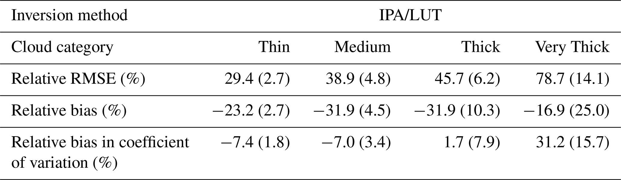
Table 4 shows the retrieval errors in optical depth distributions from the different tomographic retrievals. Retrieval errors in optical depth are substantially smaller than in the extinction field, reflecting the relatively uncorrelated spatial distribution of extinction errors. For comparison, Table 5 displays retrieval errors from an optical depth retrieval using only nadir radiance and the assumptions of the IPA; that is, it displays retrieval errors using homogeneous plane-parallel cloud models and 1D RT to generate lookup tables (LUTs) of optical depth as a function of measured radiance. Errors are substantial for the IPA retrieval, even with radiances at the same resolution as the optical depth, so that sub-pixel heterogeneity effects are absent. The IPA retrieval outperforms the default tomographic retrieval of the Very Thick clouds, but the margin is well within the ensemble standard deviations of both techniques. Moreover, even accounting for the ensemble variability, the IPA is significantly outperformed by both Restarted retrievals, which have small radiance residuals. The tomographic retrieval also outperforms the IPA retrieval when inferring the coefficient of variation in the optical depth distribution, as the IPA retrieval tends to have a bias in the estimate of the distribution width that changes sign with increasing optical depth (Iwabuchi and Hayasaka, 2002). Clearly, the tomographic retrieval demonstrated here is much more appropriate for inferring cloud optical depths in cumuliform clouds than IPA-based retrievals, even without considering the substantial benefits of retrieving the 3D distributed extinction field.
Table 4Optical depth errors for different tomographic retrievals. Means of error metrics are shown across the 10 clouds in each category with the standard deviation across the 10 clouds in parentheses. See the text for details of the error metrics.
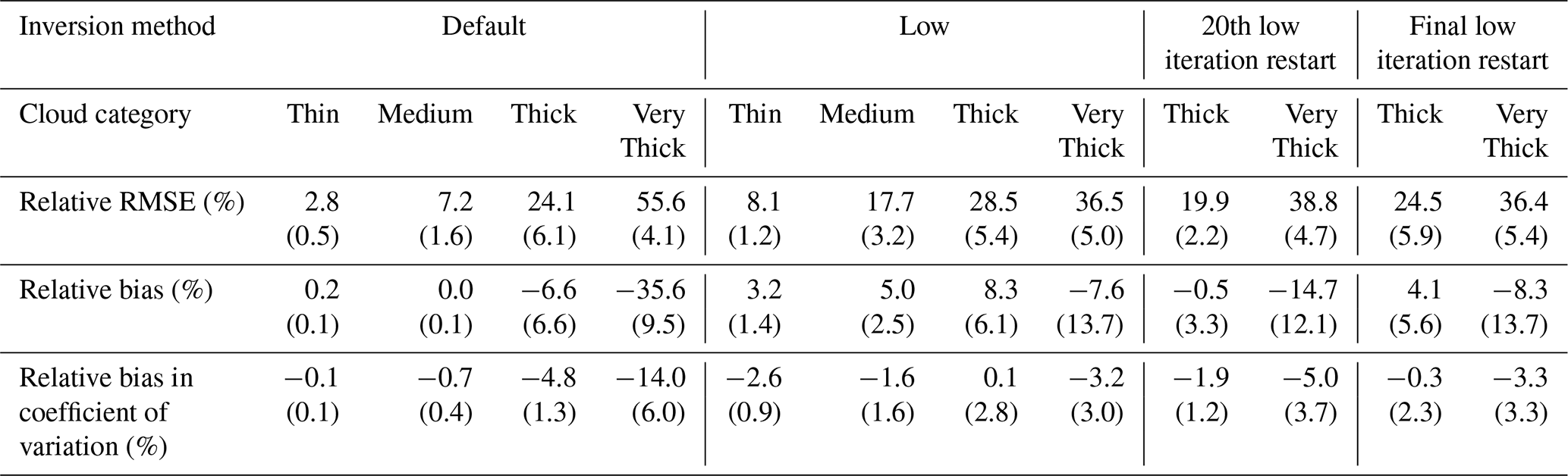
Table 5Optical depth errors for a lookup table (LUT)-based retrieval of optical depth from the nadir radiance using 1D radiative transfer. Means of error metrics are shown across the 10 clouds in each category, with the standard deviation across the 10 clouds in parentheses. See the text for details of the error metrics. The LUT uses the ground truth microphysics and is made of 20 points with linear spacing between 0 and 5 optical depths and 40 points with logarithmic spacing between 5 and 100. A cubic interpolation is used. The best-fitting optical depth is chosen using the L-BFGS-B routine. The angular accuracy used to form the LUT is the same as the ground truth 3D simulations, but a stricter splitting accuracy of 10−3 is used.
4.3 Computational expense
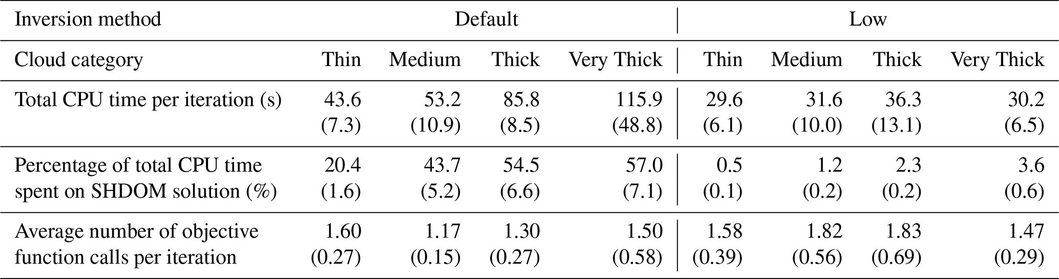
As always, it is important to also consider the computational expense of a retrieval method alongside its performance when evaluating its utility. Table 6 evaluates the computational expense of the retrievals. It shows that the use of the low-accuracy SHDOM solver in the Low retrieval almost eliminates the contribution of the RTE solver to the retrieval time, which is instead dominated by the approximate computation of the gradient and radiance calculation. This latter calculation is still unoptimized, and its cost is further discussed in Appendix F of Part 1 (Loveridge et al., 2023a). The gradient calculation is easily parallelized using multi-threading, as each observable can be evaluated independently. In our case, we parallelize using four threads. True CPU time is therefore roughly 4 times larger than wall time for this portion of the computational cost of each iteration. Computational expense is, naturally, significantly larger for the tomographic retrieval than for the IPA-based retrieval. For comparison, the tomographic retrieval is, very roughly, 2 orders of magnitude more expensive than aerosol retrievals using multi-angle radiances and the IPA assumptions with online RTE calculations, neglecting the differences in hardware (Gao et al., 2021).
Table 6Computational expense of the retrievals. Means across the 10 clouds are shown, with standard deviations across the 10 clouds in parentheses. The average cumulative Total CPU time is essentially linear in the iteration number, so the computational expense vs. accuracy trade-off of terminating the retrievals earlier can then be read from this table and Fig. 3. All computations were performed on a 2.3 GHz Intel Core i5.
Several acceleration methods are possible. The computational scaling of the SHDOM solver to larger domains using a message-passing interface (MPI)-based parallelization is documented in Pincus and Evans (2009). The solver CPU time may be decreased by using the SHDOM solution from the previous optimization iteration to initialize the next one. We utilized this feature in Part 1 to accelerate finite differencing calculations, though this method may not be stable in the presence of large changes in cloud between iterations, particularly when the adaptive grid is utilized. A more sophisticated version of this principle is to utilize a partial differential equation (PDE)-constrained optimization, which jointly refines both the inverse problem and the RTE solution at the same time, leading to orders-of-magnitude decreases in computational expense (Abdoulaev et al., 2005). The use of low-accuracy RTE solutions far from the solution appears valuable, through their ability to reduce the computational expense of the solver and increasing the convergence rate of the optimization.
The RTE solver cost may be mitigated in operational applications through the development of a statistical emulator for the SHDOM RTE solution, similar to Gao et al. (2021), though this work should likely proceed only once the retrieval algorithm is at a greater level of maturity. The convergence rate of the retrieval, and hence total computational expense, and final accuracy may also be improved through the development of preconditioning strategies. The problem of ill-conditioning in the transition to the diffuse regime has been widely recognized in diffuse optical tomography, and some mitigation strategies have been proposed (Tian et al., 2010; Niu et al., 2010). Extension of this work for a non-linear preconditioning transform (De Sterck and Howse, 2018) may be effective for our application. In our view, the computational expense of the tomography retrieval is not an oppressive limitation of the technique. Significant computational resources are routinely utilized simply to simulate analogues of the atmospheric system. The technique only calls for similar resources to be allocated to study the atmosphere as it really is.
The good performance of the retrievals of the clouds in the Thin and Medium categories is highly encouraging, as is their robustness to noise and their robustness to forward model error in this idealized scenario. Clearly, in these clouds, the approximate Jacobian is not a limiting factor in the local optimization, and the local optimization itself is a highly efficient method for performing the retrieval. While we must be careful not to extrapolate a quantitative performance from our idealized scenario to real-world conditions, we can confidently conclude that the performance of the tomography for isolated clouds within this scattering regime will be limited by forward-modelling and instrumental errors, rather than the difficulty of the inverse problem. Given that many trade cumulus clouds tend to be smaller than 800 m in geometric depth (Guillaume et al., 2018; Chazette et al., 2020) and that the average adiabatic fractions for these clouds can be significantly less than unity (Eytan et al., 2022), many of these clouds, particularly in clean conditions, will confidently have maximum optical depths of less than 40.
A minimal amount of prior information will be required to perform the retrievals of these optically thinner shallow cumulus clouds. In fact, our results cement the conclusion that small heterogeneous clouds are actually the clouds for which remote sensing using passive imaging is easiest, counter to the paradigm of 1D radiative transfer. This means that the radiance measurements themselves will provide a large amount of information that is independent of the models that might be used to form any priors, such as LESs. This is hugely encouraging, as the development of cloud tomography techniques is motivated in part by the need to develop measurements that provide independent constraints on the behaviour of LES models (Morrison et al., 2020). This fact solidifies the strengths of physics-based retrievals in comparison to statistical methods. While statistical methods trained using LES data are also attractive options to perform retrievals using 3D radiative transfer (Nataraja et al., 2022; Ronen et al., 2022), they lack a ground truth training data set and are not independent of the LESs that they may be used to evaluate.
One of the key issues that might complicate our extrapolation of the tomography performance to real clouds is the potential for cloud organization to obscure oblique views and thereby lower retrieval accuracy. Additionally, there is the issue of how the retrieval accuracy depends on the treatment of the horizontal boundary conditions and domain size. These issues have yet to be investigated systematically, requiring much larger domains, and hence computational expense, and therefore MPI-based parallelization, which is not yet implemented in AT3D. Observed statistics of cloud-to-cloud separation suggest that trade cumulus clouds are tightly spaced relative to their horizontal size and therefore thickness (Zhao and Di Girolamo, 2007). Early numerical results of radiative transfer with idealized cloud geometries show that the radiative effects of cloud–cloud interactions are significant in this regime (Weinman and Harshvardhan, 1982; Schmetz, 1984; Kobayashi, 1988). As such, investigating the sensitivity of the retrieval accuracy to cloud–cloud interactions, particularly the horizontal boundary conditions, is a high priority for establishing the efficacy of cloud tomography in more realistic conditions.
Given the success of the local optimization and approximate Jacobian in the optically thin limit, the proposed retrieval is also applicable to other optically thin scattering media such as cirrus or aerosol. For cirrus clouds, the primary barrier will likely be whether the clouds have sufficient horizontal variability for the multi-angle measurements to constrain their vertical structure. Horizontal homogeneity increases ill-conditioning, introducing ambiguity in the retrieved extinction fields (Martin and Hasekamp, 2018), though this effect is relatively minor in the optically thin limit (Loveridge et al., 2023a). Additionally, the more complex microphysical characteristics of ice and aerosols, where the shape and composition are not well known a priori, raises the question of how effective microphysical retrievals for these scatterers will be. In contrast, tomographic retrievals of liquid cloud microphysics have already been demonstrated (Levis et al., 2020) and promise to be effective in the optically thinner cumuliform clouds discussed above.
In the optically thick limit, many issues have been identified. We have provided further quantification of the degradation of retrieval accuracy and convergence in the optically thick limit due to ill-conditioning that had been previously identified (Levis et al., 2015; Martin and Hasekamp, 2018). Retrieval uncertainties are clearly large in the optically thick limit, as indicated by the significant divergences of the retrieved extinction field due to small perturbations to the measurements. However, even these perturbative estimates are tied to our choice of initialization and are not globally representative (Rodgers, 2000; Gao et al., 2022). We showed that while we can easily diagnose retrieval accuracy using the ground truth, we currently have no effective means to predict retrieval uncertainties. Developing a computationally efficient uncertainty model is a critical step in the development of the tomographic retrieval. Particle filter methods have the potential to address this need (Hu and van Leeuwen, 2021), though work is needed to verify their applicability to the tomography problem and optimize them for this application.
While global optimization methods are comprehensive, they are also much more computationally expensive than the local optimization method employed here with AT3D. Minimizing the amount of time spent in global optimization through the improvement of the local optimization is always beneficial. Correspondingly, developing more effective initialization strategies and other acceleration methods will improve the retrieval problem. Methods to estimate the order of magnitude of the optical properties within the cloud have been proposed based on either a grid search of a low-dimensional cloud model (Tzabari et al., 2022) or analytic radiative transfer results for idealized cloud geometries (Davis et al., 2021). Both of these methods require cloud envelope information as input and stereo methods have shown promise at providing the required information (Dandini et al., 2022). Other methods to retrieve the internal extinction field are also possible such as using 1D radiative transfer or heuristics based on 1D radiative transfer and linear tomography (Alexandrov et al., 2021). Both such methods neglect the asymmetry in the radiance field between forward- and backward-scattering geometries, which will lead to overestimation of the extinction field on the illuminated side of the cloud. An initialization with such an artefact would likely encourage the formation of the local minimum observed here in optically thick clouds with a gradient in extinction from the illuminated to shadowed side. Further study is needed to identify the most effective initialization methods and their range of applicability in terms of solar zenith angle and cloud optical depth.
We showed that the use of a low-accuracy forward model has been demonstrated to provide potential in accelerating retrievals. However, when angular accuracy is reduced, the retrieval problem is sufficiently non-linear that the retrievals may diverge much further than expected due to forward model error alone. This means that a low-accuracy forward model is not simply a tool to get to the same vicinity of state space quicker, at least when radiance measurements are the only constraint. While its use is beneficial for the naïve initialization used here, the benefit of using a low-accuracy forward model must be tested in combination with other initialization methods to determine whether it has general utility. Our results show that the choice of angular resolution of the forward model and phase function is an important potential source of diversity in retrieval accuracy. This parameter should be considered carefully in future studies of tomography, especially when comparing performance between studies which have used a wide variety of model configurations (Levis et al., 2015; Martin and Hasekamp, 2018; Levis et al., 2020; Doicu et al., 2022a, b).
In general, the ill-conditioning of the forward model in the optically thick limit indicates that radiance measurements alone are not sufficient to constrain the retrieval problem. There are many potential sources of prior information that could be incorporated into the tomographic retrieval, particularly in the optically thick limit. These may be from LES, simpler models or statistics from other measurements such as in situ cloud probes. The important consideration when incorporating prior data is to make sure that the resulting retrieval is used to test a hypothesis for which the prior is not relevant. For this reason, input from the wider cloud and aerosol physics communities will be invaluable in guiding the development of prior constraints for physics-based inversions or training data for statistical methods in the optically thick limit. The inclusion of other measurements such as cloud radar may also be instrumental in overcoming the limitations of the technique in optically thick clouds.
One of the main motivations for developing retrievals that use 3D radiative transfer is the need to reduce the systematic biases in the retrievals that vary with the solar and viewing geometry (Marshak et al., 2006; Kato and Marshak, 2009; Di Girolamo et al., 2010; Liang and Girolamo, 2013) and the instrument resolution (Marshak et al., 2006; Zhang et al., 2012). However, our analysis identified that systematic biases can exist in the optically thick limit that are aligned with the solar direction, despite the use of 3D radiative transfer. We hypothesize that no such biases will exist for scattering regimes that are similar to the Thin and Medium cloud categories examined here. Testing this hypothesis and quantifying the systematic variation in the biases with solar and viewing geometry and instrument resolution is an important future step in the development and validation of the retrieval.
In this study, we have evaluated an algorithm for retrieving the 3D volumetric properties of clouds using multi-angle/multi-pixel radiances and 3D RT. The retrieval utilizes an iterative, optimization-based solution to the generalized least squares problem to find a best-fitting state vector for parameterizing the cloud's structure. The retrieval, which was described in detail in Part 1, is publicly available in the software AT3D.
We evaluated the tomographic retrieval by applying it to synthetic measurements with a known ground truth. The synthetic measurements were generated from 10 stochastically generated, cumuliform clouds in (1 km)3 domains. The extinction fields of each cloud were scaled to have maximum optical depths of 4, 17.5, 44, and 88. The 3D fields of volume extinction coefficient are retrieved at 40 m resolution, which is a similar resolution to the radiance measurements (35 m).
When the target clouds have maximum optical depths less than 17, the relative RMSEs and relative biases of our idealized retrievals are less than 20 % and 1 %, respectively. Remaining errors in these clouds are limited to the small-scale (< 250 m) spatial structure of the extinction field. The relative RMSEs in the retrieved extinction field grow with the optical depth of the cloud to reach an ensemble average of ∼ 70 %, as the maximum optical thickness of the clouds reaches 88 (the value of our Very Thick cloud category). Errors become present at larger and larger spatial scales as the optical size of the cloud increases, including a notable decrease in the retrieved extinction from the illuminated to the shadowed side of the cloud and with increasing optical distance from the sensors in the optically thick clouds. This particular error pattern is attributed to the ill-posedness of the retrieval in the optically thick limit and our choice of an optically thin initialization and use of a local optimization method to solve the inverse problem.
The retrievals of clouds in the optically thick limit are highly uncertain. The addition of radiometric noise can cause large deviations in the mean extinction of individual retrievals that reach 18 % for these thick clouds, although ensemble-averaged retrieval behaviour remains unchanged. The choice of angular resolution in the forward model systematically modifies the behaviour of the retrieval result for the optically thickest clouds. Using a forward model with low angular accuracy that is less ill-conditioned results in the reduction of ensemble-averaged relative bias in the retrievals from −36 % to just −8 %, which exceeds the bias improvement from forward-modelling error alone (∼ 10 %). This highlights the importance of the angular accuracy in SHDOM for setting the numerical stability of the inverse problem. We suggest that using forward models with low angular accuracy is an avenue for improving the fidelity and computational efficiency of retrievals.
The tomographic retrieval's inference of optical depth outperforms an IPA-based retrieval of optical depth. The IPA retrieval, which uses nadir radiance here, has biases worse than −23 %. The tomographic retrieval's biases are much smaller for the clouds with optical depths less than 44 but are comparable for the thicker clouds, unless the low angular accuracy forward model is used. Relative RMSEs for the optical depth are at worst half of those of the IPA.
Overall, the proposed tomographic retrieval algorithm equipped with the approximate Jacobian calculation is the most promising for shallow cumulus cloud fields over near-black surfaces (e.g. ocean). These clouds have the richest available information content within their multi-angle reflectances, due to their highly heterogeneous nature. Therefore, from a fundamental perspective, these clouds are actually the easiest for passive tomographic remote sensing (Loveridge et al., 2022). Other optically thin clouds and aerosols are also likely to be effectively retrieved by this algorithm, which is an area for future work.
Deployment of the tomographic retrieval on the upcoming CloudCT mission (Schilling et al., 2019) has the potential to provide robust statistics of small-scale cloud properties that are unobtainable when using in situ measurements and are highly suitable for constraining model behaviour in climatically important shallow cumulus cloud fields. Further development of the retrieval is required to fully realize its potential of jointly retrieving aerosol and cloud properties and to improve its performance in more difficult, optically thicker, or stratiform cloud regimes. Future work will improve the realism of the retrieval to develop a full uncertainty model for the retrieval for evaluation against real observations.
The noise model used for the measurements uses the specifications from NASA's Request for Information (RFI) for a Tandem Stereographic Cameras instrument related to the upcoming Atmospheric Observing System (AOS) mission (NASA, 2021). The Tandem Stereographic instrument would use narrowband cameras viewing in the visible range at high spatial resolutions, with around 50 m ground instantaneous field of view (FOV) per pixel. The signal-to-noise ratio (SNR) requirement for this camera provides a reasonable proxy for the SNR that is achievable by an instrument that might be utilized for tomographic retrievals in practice. The SNR is defined as the ratio of the radiance, L, to the standard deviation of the radiance due to noise, σL. The SNR requirement for the Tandem Stereographic camera is tabulated (Table A1) as a function of the equivalent reflectance, R, which is defined in terms of the band-averaged solar irradiance, F0, and the cosine of the solar zenith angle, μ0.
The SNR model for these measurements utilizes a cubic spline to interpolate between the values. No extrapolation at the upper end of the signal range is required. To extrapolate to reflectance values below the minimum, we make the conservative assumption that the standard deviation of the radiance noise remains fixed below this reflectance level, which results in a linear decrease in the SNR until it reaches zero for no signal. This assumption is equivalent to assuming that the noise becomes dominated by dark noise below the minimum tabulated reflectance level.
The information provided is sufficient for an idealized modelling of the radiometric noise without modelling the details of the camera. We use a Poisson model to generate noise according to the SNR curve, as both the photon and dark noise are well-modelled by this stochastic process, and noise is typically limited by photon shot noise for most of the signal range. We neglect detailed models of other processes such as quantization, which are implicitly included in the required noise level.
The single parameter of the Poisson model, namely its rate, is uniquely defined as the square of the SNR. The number of counts produced in each realization of the Poisson process, NL, is scaled back to a radiance by
Table A1The signal-to-noise ratio (SNR) values tabulated as a function of equivalent reflectance used to generate noise for the measurements for the tomographic retrievals. See the text for details.
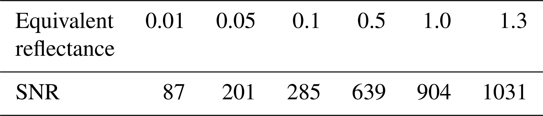
The space-carving algorithm implemented in AT3D performs a volume masking on a 3D property grid, using the 2D cloud masks and the geometric information associated with each pixel. Note that the geometric information requires not only the pixel information but also how each pixel's FOV is modelled, i.e. the geometry and weights of any sub-pixel rays. See Part 1 for how this is modelled in AT3D. The algorithm then proceeds simply by tracing each ray along its line of sight and counting the intersections of the ray with each grid point in the volume of the domain. An intersection with a grid point occurs whenever a ray intersects a grid cell for which the grid point is one of the bounding points. The intersections of clear and cloudy rays with each grid points are counted separately. A grid point is designated as cloudy by a given image if the proportion of cloudy rays intersecting it for each mono-angle image is above a specified fraction (we use 0.0 for a clearly conservative mask; Yang and Di Girolamo, 2008). If the proportion of grid point designations by each image is greater than or equal to another specified fraction (typically 1.0), then the grid point is classified as cloudy. The threshold of 1.0 ensures that all grid points are designated as cloudy, unless one view indicates that the grid point is clear. As such, the volume masking is clearly conservative.
The accuracy of a space-carving algorithm of this sort is limited in multi-angle systems by angular resolution and spatial resolution (Lee et al., 2018). It is also limited by only using binary features (i.e. the cloud masks) to retrieve structural information and therefore can only retrieve detailed information on the cloud volume when the binary cloud masks are highly structured. Other stereoscopic approaches utilizing radiance feature matching (Seiz and Davies, 2006; Veikherman et al., 2015; Bal et al., 2018) might perform better, especially in the case of stratiform clouds. However, in the case of cumuliform clouds, the performance of space carving is quite good, especially at a high spatial resolution, where the clearly conservative nature of the masking does not vastly overestimate cloud volumes.
When applied to the synthetic measurements used in the inversions, the true positive rate for grid point classification across all clouds is 10 %, the true negative rate is 65 %, the false positive rate is 25 %, and the false negative rate is 0 %. So the true clouds take up only ∼ 10 % of the domain volume, while the space-carving algorithm estimates that they take up ∼ 35 %.
In addition to the general set-up of the inversion, we must make some specific choices about the optimization algorithm. The L-BFGS-B method is sensitive to the scaling of the problem in the initial iterations, as the initial Hessian approximation in the SciPy (Virtanen et al., 2020) implementation is simply the identity matrix. The first update to the state vector is therefore simply the gradient and is therefore sensitive to the size of the initial residuals. We choose the error covariance matrix to be a diagonal matrix, with entries of to compensate this effect, where m is the number of measurements. With the solar flux chosen as unity (which sets the sizes of the radiances and residuals), this ensures that an initial step with a length of is not too small or too large in the sense that the Wolfe–Armijo conditions require. The Wolfe–Armijo conditions on the line search use the widely used default parameter values of c1=0.9 and (Byrd et al., 1995; Zhu et al., 1997).
The L-BFGS-B method has two key hyper-parameters. The first is the number of past iterations of state and gradient changes used to approximate the Hessian value of the cost function. This is chosen to be 10 iterations. The second is the maximum number of points to search in the line search during each iteration, which is also set to 10. Three stopping conditions are also specified, the maximum number of iterations is 100, the minimum allowable relative change in the cost function before termination is set to 10−8, and the smallest maximum absolute value of the gradient before termination is also 10−8. The maximum number of iterations for the Restarted retrievals is still 100, in addition to the 20 to 100 iterations at low angular accuracy used to form the initialization.
The software described and used in this paper is called Atmospheric Tomography with 3D Radiative Transfer (AT3D). A static archive of the software is available at https://doi.org/10.5281/zenodo.7062466 (Loveridge et al., 2022). The most recent version is available from https://github.com/CloudTomography/AT3D (Loveridge et al., 2023b). The original SHDOM code by Frank Evans is available from https://nit.coloradolinux.com/~evans/shdom/shdom.tar.gz (Evans, 2023).
The stochastically generated cloud fields are available from Zenodo at https://doi.org/10.5281/zenodo.8270210 (Loveridge, 2023).
JL performed the investigation and prepared the initial draft under the supervision of LDG. JL, LDG, YYS, ABD, and AL conceptualized the study. JL, AL, VH, and LF developed the software. All authors contributed to the editing of the paper.
The contact author has declared that none of the authors has any competing interests.
Publisher’s note: Copernicus Publications remains neutral with regard to jurisdictional claims in published maps and institutional affiliations.
The authors would like to thank Frank Evans for making his SHDOM code publicly available and the two anonymous referees for their valuable comments. Yoav Y. Schechner is the Mark and Diane Seiden chair in science at the Technion. He is a Landau Fellow and has been supported by the Taub Foundation. His work was conducted in the Ollendorff Minerva Center, which is funded through the BMBF. The authors are grateful to the U.S.–Israel Binational Science Foundation (BSF; grant no. 2016325) for facilitating our international collaboration.
Jesse Loveridge has been supported by NASA's FINESST programme (grant no. 80NSSC20K1633). Aviad Levis has been partially supported by the Zuckerman and Viterbi postdoctoral fellowships. This research was partially carried out at the Jet Propulsion Laboratory, California Institute of Technology, under a contract with the National Aeronautics and Space Administration (NASA; grant no. 80NM0018D0004). Anthony B. Davis has been supported by the ROSES NRA programme element (grant no. TASNPP17-0165). Larry Di Girolamo has been supported by the MISR project through the Jet Propulsion Laboratory of the California Institute of Technology (contract no. 1474871) and by NASA's ACCDAM program (contract no. 80NSSC21K1449). Linda Forster has been funded by the European Union's Framework Programme for Research and Innovation Horizon 2020 (2014–2020), under the Marie Skłodowska-Curie Actions (grant no. 754388; LMUResearchFellows), and from LMUexcellent, funded by the Federal Ministry of Education and Research (BMBF) and the Free State of Bavaria under the Excellence Strategy of the German Federal Government and States. This project has received funding from the European Union's Horizon 2020 Research and Innovation programme (grant no. 810370-ERC-CloudCT). This work received support from the U.S.–Israel Binational Science Foundation (BSF; grant no. 2016325), which facilitated this international collaboration.
This paper was edited by Alexander Kokhanovsky and reviewed by two anonymous referees.
Abdoulaev, G. S., Ren, K., and Hielscher, A. H.: Optical tomography as a PDE-constrained optimization problem, Inverse Probl., 21, 1507–1530, https://doi.org/10.1088/0266-5611/21/5/002, 2005.
Ahn, E., Huang, Y., Siems, S. T., and Manton, M. J.: A Comparison of Cloud Microphysical Properties Derived From MODIS and CALIPSO With In Situ Measurements Over the Wintertime Southern Ocean, J. Geophys. Res.-Atmos., 123, 11120–11140, https://doi.org/10.1029/2018JD028535, 2018.
Alexandrov, M. D., Emde, C., Van Diedenhoven, B., and Cairns, B.: Application of Radon Transform to Multi-Angle Measurements Made by the Research Scanning Polarimeter: A New Approach to Cloud Tomography. Part I: Theory and Tests on Simulated Data, Front. Remote Sens., 2, 791130, https://doi.org/10.3389/frsen.2021.791130, 2021.
Arridge, S. R. and Schotland, J. C.: Optical tomography: forward and inverse problems, Inverse Probl., 25, 123010, https://doi.org/10.1088/0266-5611/25/12/123010, 2009.
Bal, G.: Introduction to inverse problems, University of Chicago, https://statistics.uchicago.edu/~guillaumebal/PAPERS/IntroductionInverseProblems.pdf (last access: 21 August 2023), 2012.
Bal, G. and Jollivet, A.: Stability estimates in stationary inverse transport, Inverse Probl. Imag., 2, 427–454, https://doi.org/10.3934/ipi.2008.2.427, 2008.
Bal, G., Chen, J., and Davis, A. B.: Reconstruction of cloud geometry from high-resolution multi-angle images, Inverse Probl. Imag., 12, 261–280, https://doi.org/10.3934/ipi.2018011, 2018.
Bellouin, N., Quaas, J., Gryspeerdt, E., Kinne, S., Stier, P., Watson-Parris, D., Boucher, O., Carslaw, K. S., Christensen, M., Daniau, A.-L., Dufresne, J.-L., Feingold, G., Fiedler, S., Forster, P., Gettelman, A., Haywood, J. M., Lohmann, U., Malavelle, F., Mauritsen, T., McCoy, D. T., Myhre, G., Mülmenstädt, J., Neubauer, D., Possner, A., Rugenstein, M., Sato, Y., Schulz, M., Schwartz, S. E., Sourdeval, O., Storelvmo, T., Toll, V., Winker, D., and Stevens, B.: Bounding Global Aerosol Radiative Forcing of Climate Change, Rev. Geophys., 58, e2019RG000660, https://doi.org/10.1029/2019RG000660, 2020.
Bitterli, B., Ravichandran, S., Müller, T., Wrenninge, M., Novák, J., Marschner, S., and Jarosz, W.: A radiative transfer framework for non-exponential media, ACM T. Graphic., 37, 225, https://doi.org/10.1145/3272127.3275103, 2018.
Bruegge, C. J., Chrien, N. L., Ando, R. R., Diner, D. J., Abdou, W. A., Helmlinger, M. C., Pilorz, S. H., and Thome, K. J.: Early validation of the Multi-angle Imaging SpectroRadiometer (MISR) radiometric scale, IEEE T. Geosci. Remote, 40, 1477–1492, https://doi.org/10.1109/TGRS.2002.801583, 2002.
Byrd, R. H., Lu, P., Nocedal, J., and Zhu, C.: A Limited Memory Algorithm for Bound Constrained Optimization, SIAM J. Sci. Comput., 16, 1190–1208, https://doi.org/10.1137/0916069, 1995.
Cahalan, R. F., Ridgway, W., Wiscombe, W. J., Bell, T. L., and Snider, J. B.: The Albedo of Fractal Stratocumulus Clouds, J. Atmos. Sci., 51, 2434–2455, https://doi.org/10.1175/1520-0469(1994)051<2434:TAOFSC>2.0.CO;2, 1994.
Cahalan, R. F., Oreopoulos, L., Marshak, A., Evans, K. F., Davis, A. B., Pincus, R., Yetzer, K. H., Mayer, B., Davies, R., Ackerman, T. P., Barker, H. W., Clothiaux, E. E., Ellingson, R. G., Garay, M. J., Kassianov, E., Kinne, S., Macke, A., O'hirok, W., Partain, P. T., Prigarin, S. M., Rublev, A. N., Stephens, G. L., Szczap, F., Takara, E. E., Várnai, T., Wen, G., and Zhuravleva, T. B.: THE I3RC: Bringing Together the Most Advanced Radiative Transfer Tools for Cloudy Atmospheres, B. Am. Meteorol. Soc., 86, 1275–1294, https://doi.org/10.1175/BAMS-86-9-1275, 2005.
Cairns, B., Lacis, A. A., and Carlson, B. E.: Absorption within Inhomogeneous Clouds and Its Parameterization in General Circulation Models, J. Atmos. Sci., 57, 700–714, https://doi.org/10.1175/1520-0469(2000)057<0700:AWICAI>2.0.CO;2, 2000.
Chazette, P., Totems, J., Baron, A., Flamant, C., and Bony, S.: Trade-wind clouds and aerosols characterized by airborne horizontal lidar measurements during the EUREC4A field campaign, Earth Syst. Sci. Data, 12, 2919–2936, https://doi.org/10.5194/essd-12-2919-2020, 2020.
Chen, K., Li, Q., and Wang, L.: Stability of stationary inverse transport equation in diffusion scaling, Inverse Probl., 34, 025004, https://doi.org/10.1088/1361-6420/aa990c, 2018.
Dandini, P., Cornet, C., Binet, R., Fenouil, L., Holodovsky, V., Y. Schechner, Y., Ricard, D., and Rosenfeld, D.: 3D cloud envelope and cloud development velocity from simulated CLOUD (C3IEL) stereo images, Atmos. Meas. Tech., 15, 6221–6242, https://doi.org/10.5194/amt-15-6221-2022, 2022.
Davis, A., Marshak, A., Wiscombe, W., and Cahalan, R.: Scale Invariance of Liquid Water Distributions in Marine Stratocumulus. Part I: Spectral Properties and Stationarity Issues, J. Atmos. Sci., 53, 1538–1558, https://doi.org/10.1175/1520-0469(1996)053<1538:SIOLWD>2.0.CO;2, 1996.
Davis, A., Marshak, A., Cahalan, R., and Wiscombe, W.: The Landsat Scale Break in Stratocumulus as a Three-Dimensional Radiative Transfer Effect: Implications for Cloud Remote Sensing, J. Atmos. Sci., 54, 241–260, https://doi.org/10.1175/1520-0469(1997)054<0241:TLSBIS>2.0.CO;2, 1997.
Davis, A. B. and Marshak, A.: Photon propagation in heterogeneous optical media with spatial correlations: enhanced mean-free-paths and wider-than-exponential free-path distributions, J. Quant. Spectrosc. Ra., 84, 3–34, https://doi.org/10.1016/S0022-4073(03)00114-6, 2004.
Davis, A. B., Marshak, A., Gerber, H., and Wiscombe, W. J.: Horizontal structure of marine boundary layer clouds from centimeter to kilometer scales, J. Geophys. Res.-Atmos., 104, 6123–6144, https://doi.org/10.1029/1998JD200078, 1999.
Davis, A. B., Forster, L., Diner, D. J., and Mayer, B.: Toward Cloud Tomography from Space using MISR and MODIS: The Physics of Image Formation for Opaque Convective Clouds, arXiv [preprint], https://doi.org/10.48550/arXiv.2011.14537, 27 July 2021.
Delanoë, J. and Hogan, R. J.: A variational scheme for retrieving ice cloud properties from combined radar, lidar, and infrared radiometer, J. Geophys. Res.-Atmos., 113, D07204, https://doi.org/10.1029/2007JD009000, 2008.
De Sterck, H. and Howse, A. J. M.: Nonlinearly preconditioned L-BFGS as an acceleration mechanism for alternating least squares with application to tensor decomposition, Numer. Linear Algebr., 25, e2202, https://doi.org/10.1002/nla.2202, 2018.
Di Girolamo, L., Liang, L., and Platnick, S.: A global view of one-dimensional solar radiative transfer through oceanic water clouds, Geophys. Res. Lett., 37, L18809, https://doi.org/10.1029/2010GL044094, 2010.
Diner, D. J., Xu, F., Garay, M. J., Martonchik, J. V., Rheingans, B. E., Geier, S., Davis, A., Hancock, B. R., Jovanovic, V. M., Bull, M. A., Capraro, K., Chipman, R. A., and McClain, S. C.: The Airborne Multiangle SpectroPolarimetric Imager (AirMSPI): a new tool for aerosol and cloud remote sensing, Atmos. Meas. Tech., 6, 2007–2025, https://doi.org/10.5194/amt-6-2007-2013, 2013.
Doicu, A. and Efremenko, D. S.: Linearizations of the Spherical Harmonic Discrete Ordinate Method (SHDOM), Atmosphere, 10, 292, https://doi.org/10.3390/atmos10060292, 2019.
Doicu, A., Doicu, A., Efremenko, D., and Trautmann, T.: Cloud tomographic retrieval algorithms. I: Surrogate minimization method, J. Quant. Spectrosc. Ra., 277, 107954, https://doi.org/10.1016/j.jqsrt.2021.107954, 2022a.
Doicu, A., Doicu, A., Efremenko, D., and Trautmann, T.: Cloud tomographic retrieval algorithms. II: Adjoint method, J. Quant. Spectrosc. Ra., 285, 108177, https://doi.org/10.1016/j.jqsrt.2022.108177, 2022b.
Dubovik, O., Herman, M., Holdak, A., Lapyonok, T., Tanré, D., Deuzé, J. L., Ducos, F., Sinyuk, A., and Lopatin, A.: Statistically optimized inversion algorithm for enhanced retrieval of aerosol properties from spectral multi-angle polarimetric satellite observations, Atmos. Meas. Tech., 4, 975–1018, https://doi.org/10.5194/amt-4-975-2011, 2011.
Evans, K. F.: The Spherical Harmonics Discrete Ordinate Method for Three-Dimensional Atmospheric Radiative Transfer, J. Atmos. Sci., 55, 429–446, https://doi.org/10.1175/1520-0469(1998)055<0429:TSHDOM>2.0.CO;2, 1998.
Evans, K. F.: Spherical Harmonics Discrete Ordinate Method, University of Colorado [code], Boulder, https://nit.coloradolinux.com/~evans/shdom/shdom.tar.gz, last access: 23 March 2023.
Ewald, F., Zinner, T., Kölling, T., and Mayer, B.: Remote sensing of cloud droplet radius profiles using solar reflectance from cloud sides – Part 1: Retrieval development and characterization, Atmos. Meas. Tech., 12, 1183–1206, https://doi.org/10.5194/amt-12-1183-2019, 2019.
Ewald, F., Groß, S., Wirth, M., Delanoë, J., Fox, S., and Mayer, B.: Why we need radar, lidar, and solar radiance observations to constrain ice cloud microphysics, Atmos. Meas. Tech., 14, 5029–5047, https://doi.org/10.5194/amt-14-5029-2021, 2021.
Eytan, E., Khain, A., Pinsky, M., Altaratz, O., Shpund, J., and Koren, I.: Shallow Cumulus Properties as Captured by Adiabatic Fraction in High-Resolution LES Simulations, J. Atmos. Sci., 79, 409–428, https://doi.org/10.1175/JAS-D-21-0201.1, 2022.
Fielding, M. D., Chiu, J. C., Hogan, R. J., and Feingold, G.: A novel ensemble method for retrieving properties of warm cloud in 3-D using ground-based scanning radar and zenith radiances, J. Geophys. Res.-Atmos., 119, 10912–10930, https://doi.org/10.1002/2014JD021742, 2014.
Forster, L., Davis, A. B., Diner, D. J., and Mayer, B.: Toward Cloud Tomography from Space Using MISR and MODIS: Locating the “Veiled Core” in Opaque Convective Clouds, J. Atmos. Sci., 78, 155–166, https://doi.org/10.1175/JAS-D-19-0262.1, 2021.
Fu, D., Di Girolamo, L., Liang, L., and Zhao, G.: Regional Biases in MODIS Marine Liquid Water Cloud Drop Effective Radius Deduced Through Fusion With MISR, J. Geophys. Res.-Atmos., 124, 13182–13196, https://doi.org/10.1029/2019JD031063, 2019.
Fu, D., Di Girolamo, L., Rauber, R. M., McFarquhar, G. M., Nesbitt, S. W., Loveridge, J., Hong, Y., van Diedenhoven, B., Cairns, B., Alexandrov, M. D., Lawson, P., Woods, S., Tanelli, S., Schmidt, S., Hostetler, C., and Scarino, A. J.: An evaluation of the liquid cloud droplet effective radius derived from MODIS, airborne remote sensing, and in situ measurements from CAMP2Ex, Atmos. Chem. Phys., 22, 8259–8285, https://doi.org/10.5194/acp-22-8259-2022, 2022.
Gao, M., Franz, B. A., Knobelspiesse, K., Zhai, P.-W., Martins, V., Burton, S., Cairns, B., Ferrare, R., Gales, J., Hasekamp, O., Hu, Y., Ibrahim, A., McBride, B., Puthukkudy, A., Werdell, P. J., and Xu, X.: Efficient multi-angle polarimetric inversion of aerosols and ocean color powered by a deep neural network forward model, Atmos. Meas. Tech., 14, 4083–4110, https://doi.org/10.5194/amt-14-4083-2021, 2021.
Gao, M., Knobelspiesse, K., Franz, B. A., Zhai, P.-W., Sayer, A. M., Ibrahim, A., Cairns, B., Hasekamp, O., Hu, Y., Martins, V., Werdell, P. J., and Xu, X.: Effective uncertainty quantification for multi-angle polarimetric aerosol remote sensing over ocean, Atmos. Meas. Tech., 15, 4859–4879, https://doi.org/10.5194/amt-15-4859-2022, 2022.
Guillaume, A., Kahn, B. H., Yue, Q., Fetzer, E. J., Wong, S., Manipon, G. J., Hua, H., and Wilson, B. D.: Horizontal and Vertical Scaling of Cloud Geometry Inferred from CloudSat Data, J. Atmos. Sci., 75, 2187–2197, https://doi.org/10.1175/JAS-D-17-0111.1, 2018.
Hu, C.-C. and van Leeuwen, P. J.: A particle flow filter for high-dimensional system applications, Q. J. Roy. Meteor. Soc., 147, 2352–2374, https://doi.org/10.1002/qj.4028, 2021.
Iwabuchi, H. and Hayasaka, T.: Effects of Cloud Horizontal Inhomogeneity on the Optical Thickness Retrieved from Moderate-Resolution Satellite Data, J. Atmos. Sci., 59, 2227–2242, https://doi.org/10.1175/1520-0469(2002)059<2227:EOCHIO>2.0.CO;2, 2002.
Kato, S. and Marshak, A.: Solar zenith and viewing geometry-dependent errors in satellite retrieved cloud optical thickness: Marine stratocumulus case, J. Geophys. Res.-Atmos., 114, D01202, https://doi.org/10.1029/2008JD010579, 2009.
King, N. J. and Vaughan, G.: Using passive remote sensing to retrieve the vertical variation of cloud droplet size in marine stratocumulus: An assessment of information content and the potential for improved retrievals from hyperspectral measurements, J. Geophys. Res.-Atmos., 117, D15206, https://doi.org/10.1029/2012JD017896, 2012.
Kobayashi, T.: Parameterization of Reflectivity for Broken Cloud Fields, J. Atmos. Sci., 45, 3034–3045, https://doi.org/10.1175/1520-0469(1988)045<3034:PORFBC>2.0.CO;2, 1988.
Kutulakos, K. N. and Seitz, S. M.: A theory of shape by space carving, in: Proceedings of the Seventh IEEE International Conference on Computer Vision, Kerkyra, Greece, 20–27 September 1999, vol. 1, 307–314, https://doi.org/10.1109/ICCV.1999.791235, 1999.
Lebsock, M. and Su, H.: Application of active spaceborne remote sensing for understanding biases between passive cloud water path retrievals, J. Geophys. Res.-Atmos., 119, 8962–8979, https://doi.org/10.1002/2014JD021568, 2014.
Lee, B., Di Girolamo, L., Zhao, G., and Zhan, Y.: Three-Dimensional Cloud Volume Reconstruction from the Multi-angle Imaging SpectroRadiometer, Remote Sens., 10, 1858, https://doi.org/10.3390/rs10111858, 2018.
Levis, A., Schechner, Y. Y., Aides, A., and Davis, A. B.: Airborne Three-Dimensional Cloud Tomography, in: 2015 IEEE International Conference on Computer Vision (ICCV), Santiago, Chile, 2–13 December 2015, 3379–3387, https://doi.org/10.1109/ICCV.2015.386, 2015.
Levis, A., Schechner, Y. Y., and Davis, A. B.: Multiple-Scattering Microphysics Tomography, in: 2017 IEEE Conference on Computer Vision and Pattern Recognition (CVPR), Honolulu, HI, USA, 21–26 July 2017, 5797–5806, https://doi.org/10.1109/CVPR.2017.614, 2017.
Levis, A., Schechner, Y. Y., Davis, A. B., and Loveridge, J.: Multi-View Polarimetric Scattering Cloud Tomography and Retrieval of Droplet Size, Remote Sens., 12, 2831, https://doi.org/10.3390/rs12172831, 2020.
Lewis, G. M., Austin, P. H., and Szczodrak, M.: Spatial statistics of marine boundary layer clouds, J. Geophys. Res.-Atmos., 109, D04104, https://doi.org/10.1029/2003JD003742, 2004.
Liang, L. and Girolamo, L. D.: A global analysis on the view-angle dependence of plane-parallel oceanic liquid water cloud optical thickness using data synergy from MISR and MODIS, J. Geophys. Res.-Atmos., 118, 2389–2403, https://doi.org/10.1029/2012JD018201, 2013.
Lovejoy, S., Schertzer, D., Silas, P., Tessier, Y., and Lavallee, D.: The unified scaling model of the atmospheric dynamics and systematic analysis of scale invariance in cloud radiances, Ann. Geophys., 11, 119–127, 1993.
Loveridge, J.: AT3D-PART2: Stochastically Generated Clouds, Zenodo [data set], https://doi.org/10.5281/zenodo.8270210, 2023.
Loveridge, J., Levis, A., Aides, A., Forster, L., and Holodovsky, V.: Atmospheric Tomography with 3D Radiative Transfer, v4.1.2, Zenodo [code], https://doi.org/10.5281/zenodo.7062466, 2022.
Loveridge, J., Levis, A., Di Girolamo, L., Holodovsky, V., Forster, L., Davis, A. B., and Schechner, Y. Y.: Retrieving 3D distributions of atmospheric particles using Atmospheric Tomography with 3D Radiative Transfer – Part 1: Model description and Jacobian calculation, Atmos. Meas. Tech., 16, 1803–1847, https://doi.org/10.5194/amt-16-1803-2023, 2023a.
Loveridge, J., Levis, A., Holodovsky, V., and Forster, L.: Atmospheric Tomography with 3D Radiative Transfer, GitHub [code], https://github.com/CloudTomography/AT3D (last access: 28 March 2023), 2023b.
Marshak, A., Davis, A., Wiscombe, W., and Cahalan, R.: Radiative smoothing in fractal clouds, J. Geophys. Res.-Atmos., 100, 26247–26261, https://doi.org/10.1029/95JD02895, 1995.
Marshak, A., Davis, A., Wiscombe, W., and Cahalan, R.: Radiative effects of sub-mean free path liquid water variability observed in stratiform clouds, J. Geophys. Res.-Atmos., 103, 19557–19567, https://doi.org/10.1029/98JD01728, 1998.
Marshak, A., Platnick, S., Várnai, T., Wen, G., and Cahalan, R. F.: Impact of three-dimensional radiative effects on satellite retrievals of cloud droplet sizes, J. Geophys. Res.-Atmos., 111, D09207, https://doi.org/10.1029/2005JD006686, 2006.
Martin, W., Cairns, B., and Bal, G.: Adjoint methods for adjusting three-dimensional atmosphere and surface properties to fit multi-angle/multi-pixel polarimetric measurements, J. Quant. Spectrosc. Ra., 144, 68–85, https://doi.org/10.1016/j.jqsrt.2014.03.030, 2014.
Martin, W. G. K. and Hasekamp, O. P.: A demonstration of adjoint methods for multi-dimensional remote sensing of the atmosphere and surface, J. Quant. Spectrosc. Ra., 204, 215–231, https://doi.org/10.1016/j.jqsrt.2017.09.031, 2018.
Miller, D. J., Zhang, Z., Platnick, S., Ackerman, A. S., Werner, F., Cornet, C., and Knobelspiesse, K.: Comparisons of bispectral and polarimetric retrievals of marine boundary layer cloud microphysics: case studies using a LES–satellite retrieval simulator, Atmos. Meas. Tech., 11, 3689–3715, https://doi.org/10.5194/amt-11-3689-2018, 2018.
Morrison, H., van Lier-Walqui, M., Fridlind, A. M., Grabowski, W. W., Harrington, J. Y., Hoose, C., Korolev, A., Kumjian, M. R., Milbrandt, J. A., Pawlowska, H., Posselt, D. J., Prat, O. P., Reimel, K. J., Shima, S.-I., van Diedenhoven, B., and Xue, L.: Confronting the Challenge of Modeling Cloud and Precipitation Microphysics, J. Adv. Model. Earth Syst., 12, e2019MS001689, https://doi.org/10.1029/2019MS001689, 2020.
Nakajima, T. and Tanaka, M.: Algorithms for radiative intensity calculations in moderately thick atmospheres using a truncation approximation, J. Quant. Spectrosc. Ra., 40, 51–69, https://doi.org/10.1016/0022-4073(88)90031-3, 1988.
NASA: AtmOS Tandem Stereographic Cameras Instrumentation, National Aeronautics and Space Administration, Goddard Space Flight Center, https://aos.gsfc.nasa.gov/docs/ATMOS_Tandem_Stereographic_Cameras_210602+final+revised.pdf, last access: 8 June 2021.
Nataraja, V., Schmidt, S., Chen, H., Yamaguchi, T., Kazil, J., Feingold, G., Wolf, K., and Iwabuchi, H.: Segmentation-based multi-pixel cloud optical thickness retrieval using a convolutional neural network, Atmos. Meas. Tech., 15, 5181–5205, https://doi.org/10.5194/amt-15-5181-2022, 2022.
Niu, H., Lin, Z.-J., Tian, F., Dhamne, S., and Liu, H.: Comprehensive investigation of three-dimensional diffuse optical tomography with depth compensation algorithm, J. Biomed. Opt., 15, 046005, https://doi.org/10.1117/1.3462986, 2010.
Painemal, D., Spangenberg, D., Smith Jr., W. L., Minnis, P., Cairns, B., Moore, R. H., Crosbie, E., Robinson, C., Thornhill, K. L., Winstead, E. L., and Ziemba, L.: Evaluation of satellite retrievals of liquid clouds from the GOES-13 imager and MODIS over the midlatitude North Atlantic during the NAAMES campaign, Atmos. Meas. Tech., 14, 6633–6646, https://doi.org/10.5194/amt-14-6633-2021, 2021.
Peherstorfer, B., Willcox, K., and Gunzburger, M.: Survey of Multifidelity Methods in Uncertainty Propagation, Inference, and Optimization, SIAM Rev., 60, 550–591, https://doi.org/10.1137/16M1082469, 2018.
Pincus, R. and Evans, K. F.: Computational Cost and Accuracy in Calculating Three-Dimensional Radiative Transfer: Results for New Implementations of Monte Carlo and SHDOM, J. Atmos. Sci., 66, 3131–3146, https://doi.org/10.1175/2009JAS3137.1, 2009.
Prigarin, S. M. and Marshak, A.: A Simple Stochastic Model for Generating Broken Cloud Optical Depth and Cloud-Top Height Fields, J. Atmos. Sci., 66, 92–104, https://doi.org/10.1175/2008JAS2699.1, 2009.
Raveendran, T., Gupta, S., Vasu, R. M., and Roy, D.: Pseudo-time particle filtering for diffuse optical tomography, J. Opt. Soc. Am. A, 28, 2070–2081, https://doi.org/10.1364/JOSAA.28.002070, 2011.
Rodgers, C. D.: Inverse Methods for Atmospheric Sounding, World Scientific, https://doi.org/10.1142/3171, 2000.
Ronen, R., Holodovsky, V., and Schechner, Y. Y.: Variable Imaging Projection Cloud Scattering Tomography, IEEE T. Pattern Anal., 1–12, https://doi.org/10.1109/TPAMI.2022.3195920, 2022.
Schilling, K., Schechner, Y. Y., and Koren, I.: CloudCT – Computed Tomography Of Clouds By A Small Satellite Formation, 12th IAA symposium on Small Satellites for Earth Observation, Berlin, Germany, 6–10 May 2019, https://www.cloudct.space/_files/ugd/aef793_e2334d0332014022aeb4a5891ff12e92.pdf (last access: 20 March 2023), 2019.
Schmetz, J.: On the parameterization of the radiative properties of broken clouds, Tellus A, 36, 417–432, https://doi.org/10.3402/tellusa.v36i5.11644, 1984.
Seiz, G. and Davies, R.: Reconstruction of cloud geometry from multi-view satellite images, Remote Sens. Environ., 100, 143–149, https://doi.org/10.1016/j.rse.2005.09.016, 2006.
Sherwood, S. C., Bony, S., and Dufresne, J.-L.: Spread in model climate sensitivity traced to atmospheric convective mixing, Nature, 505, 37–42, https://doi.org/10.1038/nature12829, 2014.
Sherwood, S. C., Webb, M. J., Annan, J. D., Armour, K. C., Forster, P. M., Hargreaves, J. C., Hegerl, G., Klein, S. A., Marvel, K. D., Rohling, E. J., Watanabe, M., Andrews, T., Braconnot, P., Bretherton, C. S., Foster, G. L., Hausfather, Z., von der Heydt, A. S., Knutti, R., Mauritsen, T., Norris, J. R., Proistosescu, C., Rugenstein, M., Schmidt, G. A., Tokarska, K. B., and Zelinka, M. D.: An Assessment of Earth's Climate Sensitivity Using Multiple Lines of Evidence, Rev. Geophys., 58, e2019RG000678, https://doi.org/10.1029/2019RG000678, 2020.
Shi, H.-J. M., Xie, Y., Byrd, R., and Nocedal, J.: A Noise-Tolerant Quasi-Newton Algorithm for Unconstrained Optimization, arXiv [preprint], https://doi.org/10.48550/arXiv.2010.04352, 9 September 2021.
Tarvainen, T., Kolehmainen, V., Pulkkinen, A., Vauhkonen, M., Schweiger, M., Arridge, S. R., and Kaipio, J. P.: An approximation error approach for compensating for modelling errors between the radiative transfer equation and the diffusion approximation in diffuse optical tomography, Inverse Probl., 26, 015005, https://doi.org/10.1088/0266-5611/26/1/015005, 2009.
Tian, F., Niu, H., Khadka, S., Lin, Z.-J., and Liu, H.: Algorithmic depth compensation improves quantification and noise suppression in functional diffuse optical tomography, Biomed. Opt. Express, 1, 441–452, https://doi.org/10.1364/BOE.1.000441, 2010.
Tzabari, M., Holodovsky, V., Shubi, O., Eytan, E., Koren, I., and Schechner, Y. Y.: Settings for Spaceborne 3-D Scattering Tomography of Liquid-Phase Clouds by the CloudCT Mission, IEEE T. Geosci. Remote, 60, 1–16, https://doi.org/10.1109/TGRS.2022.3198525, 2022.
van Leeuwen, P. J., Künsch, H. R., Nerger, L., Potthast, R., and Reich, S.: Particle filters for high-dimensional geoscience applications: A review, Q. J. Roy. Meteor. Soc., 145, 2335–2365, https://doi.org/10.1002/qj.3551, 2019.
Veikherman, D., Aides, A., Schechner, Y. Y., and Levis, A.: Clouds in the Cloud, in: Computer Vision – ACCV 2014, Springer, Cham, 659–674, https://doi.org/10.1007/978-3-319-16817-3_43, 2015.
Virtanen, P., Gommers, R., Oliphant, T. E., Haberland, M., Reddy, T., Cournapeau, D., Burovski, E., Peterson, P., Weckesser, W., Bright, J., van der Walt, S. J., Brett, M., Wilson, J., Millman, K. J., Mayorov, N., Nelson, A. R. J., Jones, E., Kern, R., Larson, E., Carey, C. J., Polat, İ., Feng, Y., Moore, E. W., VanderPlas, J., Laxalde, D., Perktold, J., Cimrman, R., Henriksen, I., Quintero, E. A., Harris, C. R., Archibald, A. M., Ribeiro, A. H., Pedregosa, F., and van Mulbregt, P.: SciPy 1.0: fundamental algorithms for scientific computing in Python, Nat. Methods, 17, 261–272, https://doi.org/10.1038/s41592-019-0686-2, 2020.
Weinman, J. A. and Harshvardhan: Solar reflection from a regular array of horizontally finite clouds, Appl. Optics, 21, 2940–2944, https://doi.org/10.1364/AO.21.002940, 1982.
Wiscombe, W. J.: The Delta–M Method: Rapid Yet Accurate Radiative Flux Calculations for Strongly Asymmetric Phase Functions, J. Atmos. Sci., 34, 1408–1422, https://doi.org/10.1175/1520-0469(1977)034<1408:TDMRYA>2.0.CO;2, 1977.
Xu, Z., Mace, G. G., and Posselt, D. J.: Impact of Rain on Retrieved Warm Cloud Properties Using Visible and Near-Infrared Reflectances Using Markov Chain Monte Carlo Techniques, IEEE T. Geosci. Remote, 60, 1–10, https://doi.org/10.1109/TGRS.2022.3208007, 2022.
Yang, Y. and Di Girolamo, L.: Impacts of 3-D radiative effects on satellite cloud detection and their consequences on cloud fraction and aerosol optical depth retrievals, J. Geophys. Res.-Atmos., 113, D04213, https://doi.org/10.1029/2007JD009095, 2008.
Zhang, Z., Ackerman, A. S., Feingold, G., Platnick, S., Pincus, R., and Xue, H.: Effects of cloud horizontal inhomogeneity and drizzle on remote sensing of cloud droplet effective radius: Case studies based on large-eddy simulations, J. Geophys. Res.-Atmos., 117, D19208, https://doi.org/10.1029/2012JD017655, 2012.
Zhao, G. and Di Girolamo, L.: Statistics on the macrophysical properties of trade wind cumuli over the tropical western Atlantic, J. Geophys. Res.-Atmos., 112, D10204, https://doi.org/10.1029/2006JD007371, 2007.
Zhao, H. and Zhong, Y.: Instability of an Inverse Problem for the Stationary Radiative Transport Near the Diffusion Limit, SIAM J. Math. Anal., 51, 3750–3768, https://doi.org/10.1137/18M1222582, 2019.
Zhu, C., Byrd, R. H., Lu, P., and Nocedal, J.: Algorithm 778: L-BFGS-B: Fortran subroutines for large-scale bound-constrained optimization, ACM Trans. Math. Softw., 23, 550–560, https://doi.org/10.1145/279232.279236, 1997.