Quality evaluation for measurements of wind field and turbulent fluxes from a UAV-based eddy covariance system

Instrumentation packages for eddy covariance (EC) measurements have been developed for unoccupied aerial vehicles (UAVs) to measure the turbulent fluxes of latent heat (LE), sensible heat (H), and CO₂ (F_c) in the atmospheric boundary layer. This study aims to evaluate the performance of this UAV-based EC system. First, the measurement precision (1σ) of georeferenced wind was estimated to be 0.07 m s⁻¹. Then, the effect of the calibration parameter and aerodynamic characteristics of the UAV on wind measurement was examined by conducting a set of calibration flights. The results showed that the calibration improved the quality of the measured wind field, and the influence of upwash and the leverage effect can be ignored in wind measurement by the UAV. Third, for the measurements of turbulent fluxes, the error caused by instrumental noise was estimated to be 0.03 $\mathrm{\mu }\mathrm{mol}{\mathrm{m}}^{-\mathrm{2}}{\mathrm{s}}^{-\mathrm{1}}$ for F_c, 0.02 W m⁻² for H, and 0.08 W m⁻² for LE. Fourth, data from the standard operational flights were used to assess the influence of resonance on the measurements and to test the sensitivity of the measurement under the variation (±30 %) in the calibration parameters around their optimum value. The results showed that the effect of resonance mainly affected the measurement of CO₂ (∼5 %). The pitch offset angle (ε_θ) significantly affected the measurement of vertical wind (∼30 %) and turbulent fluxes (∼15 %). The heading offset angle (ε_ψ) mainly affected the measurement of horizontal wind (∼15 %), and other calibration parameters had no significant effect on the measurements. The results lend confidence to the use of the UAV-based EC system and suggest future improvements for the optimization of the next-generation system.

1 Introduction

In environmental, hydrological, and climate change sciences, flux measurement at the regional scale (level of several to tens of kilometers) is a pressing problem (Mayer et al., 2022; Chandra et al., 2022). Process-based or remote-sensing-based (RS) models are often used to estimate land surface fluxes in matter and energy from continental to global scales with a typical spatial resolution of 1–10 km (Hu and Jia, 2015; Mohan et al., 2020; Liu et al., 1999). However, observational data, especially at similar scales to models' estimates, are often lacking, which presents a significant challenge for the validation and evaluation of the surface flux products from these models' estimates (Li et al., 2018, 2017). On the ground, in the past few decades, extensive eddy covariance (EC) flux sites with their composed networks and optical-microwave scintillometer (OMS) sites have been built to provide temporally continuous monitoring of surface flux at local (hundreds of meters around the measurement site of ground EC) and path (a distance of a few hundred meters to nearly 10 km between the transmitter and receiver terminal of OMS) scales (Yang et al., 2017; Liu et al., 2018; Zhang et al., 2021; Zheng et al., 2023). However, flux from ground measurements needs to be scaled up to kilometer scale to provide comparable surface “relative-truth” flux data for the process- or RS-based models at larger spatial scales (Liu et al., 2016). But the spatial density of these flux measurement sites is still low compared to the heterogeneity in surface fluxes, which means that major scaling bias may exist in the upscaled flux data (Wang et al., 2016; Li et al., 2021). Therefore, regional-scaled oriented flux measurement techniques need to be developed to complement the missing scale between these ground- and model-based approaches (Chu et al., 2021).

An aircraft-based EC flux measurement method, which has been developed for turbulence measurements for more than 40 years (Lenschow et al., 1980; Desjardins et al., 1982), is considered to be the optimum method for measuring turbulent flux at regional scales (several hundred square kilometers) (Gioli et al., 2004; Garman et al., 2006). To date, several types of aircraft, including occupied or unoccupied fixed-wing aircraft, delta-wing aircraft, and helicopters, have been used for measurements of turbulent flux by equipping them with the EC sensors to measure three-dimensional (3D) wind, air temperature, and gas concentrations at a high frequency (Gioli et al., 2006; Metzger et al., 2012; Wolfe et al., 2018; Sun et al., 2021a; Reuter et al., 2021). Among them, fixed-wing aircraft and delta-wing aircraft are better airborne platforms for EC measurements compared to helicopters due to their tightly coupled structure with the wind sensor and because their flow distortion around the fuselage can more easily be avoided or modeled (Prudden et al., 2018; Garman et al., 2008). A wide range of occupied aircraft has been developed to measure turbulent flux, including single-engine light aircraft (e.g., Sky Arrow 650, Long-EC, weight-shift microlight aircraft) (Gioli et al., 2006; Crawford and Dobosy, 1992; Metzger et al., 2012), twin-engine aircraft (e.g., Twin Otter, NASA Carbon Airborne Flux Experiment) (Desjardins et al., 2016; Wolfe et al., 2018), and larger quad-engine utility aircraft (e.g., NOAA WP-3D Orion aircraft) (Khelif et al., 1999). These airborne flux measurements, in combination with ground EC measurements, provide an excellent opportunity to produce regional-scaled, spatiotemporal, continuous surface flux datasets that can improve our understanding of the processes of land–atmosphere interactions in regional and global changes (Chen et al., 1999; Prueger et al., 2005; Calmer et al., 2019; Tadić et al., 2021). However, occupied aircraft are expensive to operate and maintain. Aviation safety and operational regulations require that occupied aircraft must fly above a minimum altitude (400 m above the highest elevation within 25 km on each side of the center line of the air route in China) and must avoid hazardous conditions such as icing or severe turbulence. The flow distortion induced by the aircraft itself (from the wings, fuselage, and the propellers) complicates the wind vector measurement from the aircraft platform, which means that sophisticated correction procedures should be applied to correct for the flow distortion effects (Elston et al., 2015; Williams and Marcotte, 2000; Drüe and Heinemann, 2013).

In recent years, there has been a rapidly growing interest in unoccupied aerial vehicle (UAV) platforms for atmospheric research, especially because of their lower construction, operation, and maintenance costs compared with occupied platforms. High-performance fixed-wing UAVs offer a high payload capacity (5–10 kg) and similar endurance (2–3 h) and operating altitude (3500 m or higher above sea level) to occupied aircraft but with much less turbulence disturbance due to their small fuselage size (Reineman et al., 2013). More importantly, the advancements in small, fast, and powerful sensors and microprocessors make it possible to use UAVs for comprehensive atmospheric measurements (Sun et al., 2021a). Several types of UAVs with different atmospheric measurement objectives have been developed and deployed, ranging from small (e.g., 140 g small unoccupied meteorological observer) to medium (e.g., 1.5 kg meteorological mini unoccupied aerial vehicle, 1.0 kg multi-purpose automatic sensor carrier) and large (e.g., 6.8 kg Manta, 5.6 kg ScanEagle) (Reuder et al., 2016; Båserud et al., 2016; Reineman et al., 2013; Zappa et al., 2020). A comprehensive overview of these UAVs for atmospheric measurement can be found in Elston et al. (2015) and Sun et al. (2021a). For turbulence measurement, the UAVs were equipped with a commercial or custom multi-hole (five- or nine-hole) probe paired with an integrated navigation system (INS) to obtain the wind vector. Small and medium UAVs could typically only measure fast 3D wind vectors and air temperature fluctuations for measurements of momentum and sensible heat flux, whereas large UAVs were equipped with more types (e.g., radiation, optics, or gas concentration) and more accurate sensors for the measurement of more types of meteorological properties, including sensible and latent heat fluxes, CO₂ fluxes, and radiation fluxes, as well as surface properties (Reineman et al., 2013; Sun et al., 2021a). UAVs can be deployed in a variety of application environments and complex conditions, which offer distinct advantages over occupied aircraft in their ability to safely perform measurements in low-altitude conditions (below 100 m above ground level) and greatly reduce operational costs (Witte et al., 2017). Anderson and Gaston (2013) predict that UAVs will revolutionize spatial data collection in ecology and meteorology.

The EC method is a well-developed technology for directly measuring vertical turbulent flux (fluxes of sensible heat, latent heat, and CO₂) within the atmospheric boundary layers (ABLs) (Peltola et al., 2021). It requires accurate time (for the ground tower) or spatial (for the mobile platform) series of both the transported scalar quantity and the transporting turbulent wind. Each should be measured at sufficient frequency to resolve the flux contribution from small eddies (Vellinga et al., 2013). However, the measurement of the georeferenced 3D wind vector, which is a prerequisite for EC measurements, is challenging for airborne platforms. The georeferenced 3D wind measured by airborne platforms is the vector sum of the aircraft velocity relative to the earth (inertial velocity) and the velocity relative to the air (relative wind vector or true airspeed). Therefore, accurate measurements of the relative wind as well as the motion and attitude of the platform are essential to accurately measure the georeferenced wind vector and the turbulent flux (Metzger et al., 2011). Garman et al. (2006) estimated the measurement precision (1σ) of the vertical wind measurements of a commercial nine-hole turbulence probe (known as the Best Air Turbulence probe, often abbreviated as BAT probe) to be 0.03 m s⁻¹ by combining the precision of the BAT probe and the integrated navigation system. A light delta-wing EC flux measurement aircraft developed by Metzger et al. (2011) reported a 1σ precision of wind measurement of 0.09 m s⁻¹ for horizontal wind and 0.04 m s⁻¹ for vertical wind using a specially customized five-hole probe (5HP). On this basis, in combination with a commercial infrared gas analyzer, the 1σ precision of flux measurement was 0.003 m s⁻¹ for friction velocity, 0.9 W m⁻² for sensible heat flux, and 0.5 W m⁻² for latent heat flux (Metzger et al., 2012). The EC flux measurement from a UAV platform can now be achieved with a similar reliability to an occupied platform. The Manta and ScanEagle UAV-based EC measurements developed by Reineman et al. (2013) achieved precise wind measurements (0.05 m s⁻¹ for horizontal and 0.02 m s⁻¹ for vertical wind) using a custom nine-hole probe and a commercial high-precision integrated navigation system (INS). However, the onboard instrument packages for the Manta and ScanEagle UAVs are independent of each other in their measurements of turbulent and radiation fluxes, and the CO₂ flux measurement is lacking.

Inspired by these studies, Sun et al. (2021a) used a high-performance fuel-powered vertical takeoff and landing (VTOL) fixed-wing UAV platform to integrate the scientific payloads for EC and radiation measurements to obtain a comprehensive measurement of turbulent and radiation fluxes. This UAV-based EC system could measure turbulent fluxes of sensible heat, latent heat, and CO₂, as well as radiation fluxes including net radiation and upward- and downward-looking photosynthetically active radiation (PAR). This system was successfully tested in Inner Mongolia, China, and was applied to measure the regional sensible and latent heat fluxes in the Yancheng coastal wetland in Jiangsu, China (Sun et al., 2021a, b). During these field studies, the UAV-based EC measurements achieved a near-consistent observational result compared with ground EC measurements (Sun et al., 2021b). However, some shortcomings in the developed UAV-based EC system were also identified. In particular, the noise effects from the engine and propeller were not fully isolated, resulting in high-frequency noise in the measured scalars (air temperature as well as H₂O and CO₂ concentrations). This UAV-based EC system is continuously being improved (in Sect. 2.1). However, no quantitative evaluations of the measurement precision of the wind field and turbulent flux as well as of the influence of the resonance noise from the UAV operation have been made yet. Previous work using ground EC as a benchmark to assess the measurement performance of the UAV-based EC system has been disputed due to differences in EC sensors, platforms, measurement height, and source areas (i.e., footprint), as well as the influence of surface heterogeneity, flux divergence, the inversion layer, and the stochastic nature of turbulence (Sun et al., 2021b; Wolfe et al., 2018; Hannun et al., 2020).

This study attempts to evaluate the performance of the UAV-based EC system developed by Sun et al. (2021a) in the measurements of wind field and turbulent fluxes. For these purposes, data from two field measurement campaigns, including a set of calibration flights and some standard operational flights, were used in this study. First, the current study investigated the quality of the measurement of the georeferenced wind vector, including measurement error (1σ), and the improvements for wind measurement after system calibration. Second, using the measured data from standard operational flights, the flux measurement error related to instrumental noise was estimated with a method proposed by Billesbach (2011). Errors propagated through the correction terms (i.e., Webb–Pearman–Leuning (WPL) correction for latent heat and CO₂ flux) were also included in our analysis (Webb et al., 1980; Kowalski et al., 2021). Then, the impacts of resonance noise on the measured scalar variance and the flux covariance were also estimated by comparing the real (co)spectral curve with the theoretical reference curve from Massman and Clement (2005). Lastly, the sensitivity of the measured georeferenced wind vector and turbulent flux to the errors in the calibration parameters (determined by the calibration flight) were assessed by adding an error of ±30 % to their calibrated value.

2 Materials and methods

2.1 The UAV-based EC system

The VTOL fixed-wing UAV platform used for EC measurement has minimal requirements for the takeoff location and offers a high payload capacity of up to 10 kg. This UAV has a wingspan of 3.7 m, a fuselage length of 2.85 m, and a maximum takeoff weight of 60 kg. The UAV engine is mounted in a pusher configuration, allowing for the turbulence probe to be installed directly on the nose of the UAV, minimizing or eliminating airflow contamination due to upwash and sidewash generated by the wings (Crawford et al., 1996). Control of the UAV is totally autonomous, and the pilots have the option to enable manual control in emergency conditions. The UAV has a cruise flight speed of 28 to 31 m s⁻¹ with an endurance of almost 3 h, and it has a flight ceiling of up to 3800 m above sea level. Detailed information about this UAV can be found in Sun et al. (2021a).

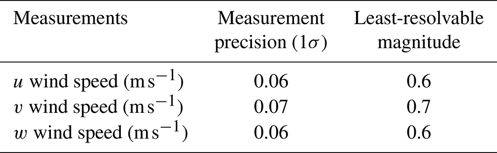
The flux payloads of the UAV-based EC system include a precision-engineered five-hole pressure probe (5HP) for measurement of the true airspeed as well as the attack (α) and sideslip (β) angles of the incoming flow relative to the UAV, a dual-antenna integrated navigation system (INS) for high-accuracy measurement of UAV ground speed and attitude, an open-path infrared gas analyzer (IRGA) for recording the gas concentrations of CO₂ and water vapor, a fast temperature sensor for measurement of the fast temperature fluctuations, and a slow-response temperature probe for providing a mean air temperature reference. The sensor modules and their 1σ precision of the measured variables related to EC measurement are listed in Table 1. For the 5HP, the 1σ measurement precision was acquired from the wind tunnel test after wind tunnel calibration (Sun et al., 2021a).

Table 1 Summary of the sensor modules, measured variables, and their measurement precision used to determine the georeferenced wind velocity and turbulent flux.

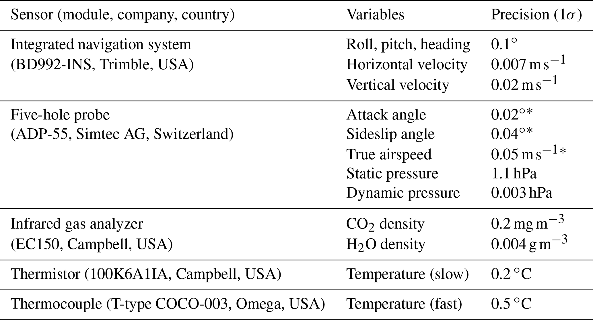
^∗ Results from the wind tunnel test.

The sample rate of EC measurement is 50 Hz, except for the slow-response temperature probe (1 Hz), yielding a turbulence horizontal resolution of approximately 1.2 m at a cruising speed of 30 m s⁻¹. The system was improved according to deficiencies identified after several field measurements with the following adjustments: (1) a laser distance measurement unit was mounted for measuring the distance between the UAV and the ground level, (2) the platinum resistance thermometer was replaced by a thermocouple (Omega T-type COCO-003; ∅0.075 mm) for improving the resistance of the high-frequency temperature measurements to vibration noise from the engine, (3) the vibration isolator structure of the IRGA was improved, and (4) the original data logger (CR1000X, Campbell, USA) was replaced with a lighter one (CR6, Campbell, USA). All the digital and analogue signals from the sensor modules are stored and synchronized by the onboard data logger, and the onboard scientific payloads are designed to be isolated from the electronic components of the UAV to ensure that any problems that occur would not jeopardize the safety of flying (Sun et al., 2021a).

2.2 Field campaign

2.2.1 In-flight calibration campaign

In order to calibrate the mounting error in the 5HP of the UAV-based EC system, an in-flight calibration campaign was carried out on 4 September 2022 at the Caofeidian shoal harbor in the Bohai Sea of northern China. At low tide, a large area of the tidal flat is exposed, while at high tide, only the barrier islands are visible (Xu et al., 2021). The assumption conditions should be satisfied for the calibration flight, including (1) low-turbulence transport conditions (i.e., no disturbance), (2) a constant mean horizontal wind, and (3) mean vertical wind near 0 (Drüe and Heinemann, 2013; Vellinga et al., 2013; Van Den Kroonenberg et al., 2008). This allows for identical wind components for several consecutive straights in opposite or vertical flight directions. These assumptions are usually well satisfied above the ABL or under stable atmospheric conditions (Drüe and Heinemann, 2013). Over the sea surface, due to its uniform- and cool-surface properties, the turbulence fluctuations are weaker than those over the land surface (Mathez and Smerdon, 2018), making it a more ideal environment for conducting calibration flights.

The in-flight calibration campaign in this study included three flight maneuvers: the “box” maneuver, the “racetrack” maneuver, and the “acceleration–deceleration” maneuver. The trajectories of these flight maneuvers are shown in Fig. 1. The calibration flight was executed between 07:28 and 07:48 (Beijing time), and the average flight altitude was 400 m ($\mathit{\sigma }=\pm \mathrm{0.78}$ m) above sea level. Considering the uniform and cool underlying surface and the stable atmospheric conditions of the early morning, we assume no disturbance from the underlying surface during the calibration flight, and the assumptions for the calibration flight are satisfied.

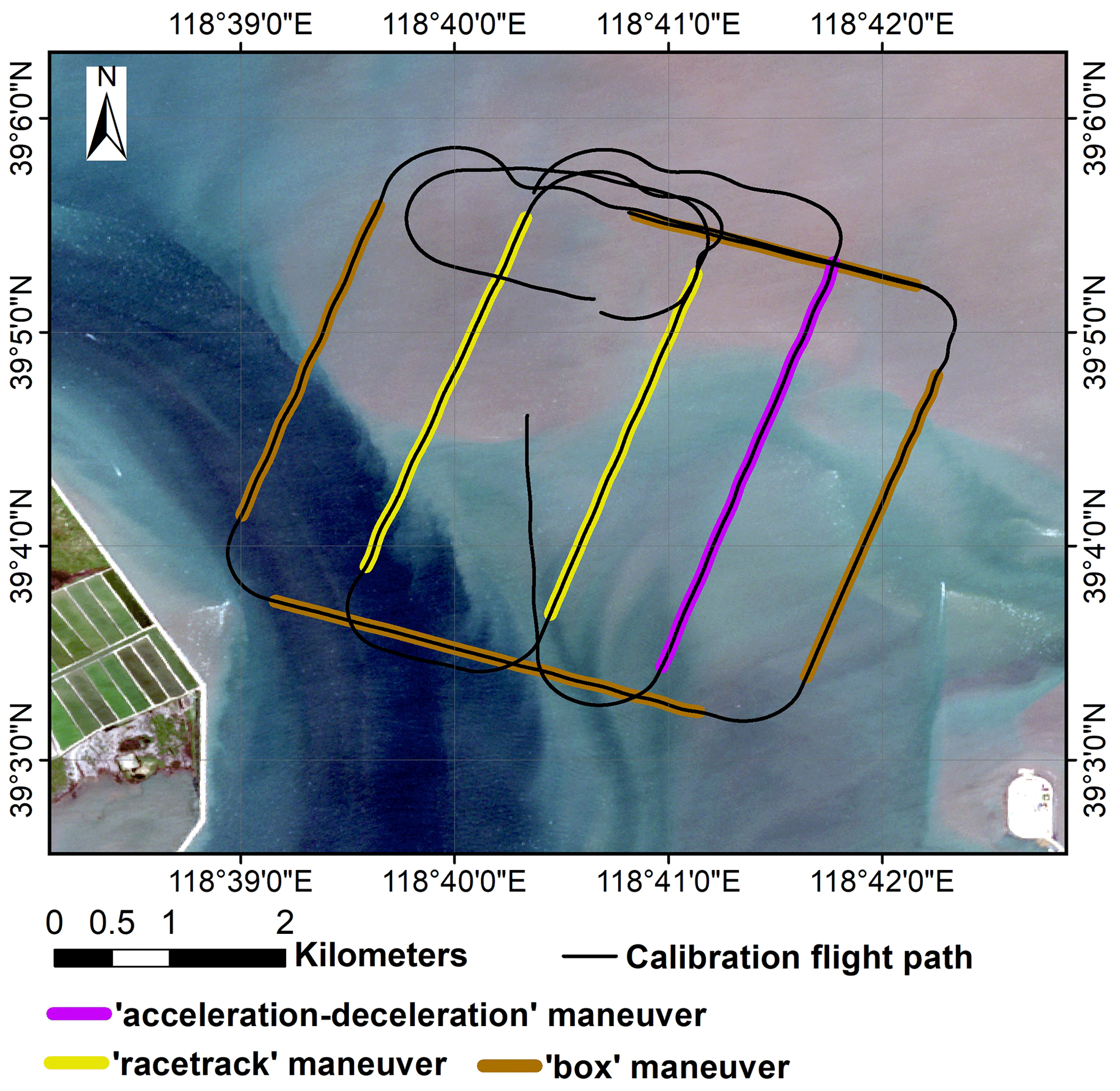
Figure 1 Flight trajectories of the calibration flight campaign carried out on 4 September 2022 at the Caofeidian shoal harbor in the Bohai Sea of northern China. The land surface image is from the Sentinel-2A satellite image, with the true color combination acquired on 1 September 2022.

The box maneuver (brown line in Fig. 1) is used to determine the mounting misalignment angle in the heading (ϵ_ψ) and pitch (ϵ_θ) between the 5HP and the center of gravity (CG) of the UAV. The flight path is a box in which the four straight legs are flown at a constant cruising speed, flight altitude, and heading for 2 continuous minutes. The racetrack maneuver (yellow line in Fig. 1) is used to evaluate the quality of the calibration parameters acquired from the previous box maneuver. The flight path consists of two parallel straight flight tracks connected by one 180^∘ turn. Each straight flight section lasts 2 min at a constant speed and flight altitude. Lastly, the acceleration–deceleration maneuver (purple line in Fig. 1) is used to check the influence of lift-induced upwash from the wing to the measured attack angle by the 5HP. During this maneuver, the aircraft is kept straight and level at a constant pressure altitude. When beginning this maneuver, the aircraft accelerates to its maximum airspeed (35 m s⁻¹). Then, the airspeed gradually reduces to near its minimum airspeed (25 m s⁻¹) and back up to its maximum airspeed. The pressure altitude of the aircraft is maintained throughout this maneuver, and the entire maneuver lasts 1 min. This maneuver creates a series of continuous changed pitch (θ) and attack (α) angles. If the relationship between the incident flow attack angles (α) measured by the 5HP and the pitch angle measured by the INS is close to 1:1, it indicates that the effect from the fuselage-induced flow distortion on the wind measurements is negligible (Garman et al., 2006).

2.2.2 Standard operational flight campaign

The reliability of the EC measurement from UAVs is susceptible to several factors, mainly including instrumental noise, resonance noise, and the quality of the calibration parameter, etc. In order to evaluate the flux measurement error related to instrumental noise and the effects of resonance on the measured scalar and to investigate the sensitivity of the measured georeferenced wind vector and turbulent flux to uncertainty in the calibration parameter, we used data from seven flights in the Binhai New Area in Tianjin, China, between 8 and 16 August 2022. This area is located in the west coast of the Bohai Sea and is a coastal alluvial plain with altitudes between 1 and 3 m (Chen et al., 2017). The flight path, shown in Fig. 2, includes three parallel transect lines of approximately 4 km in length each and at 1–2 km intervals. All flights occurred during the daytime and were performed in the same trajectory at a low altitude of about 90 m above sea level. The flight area covered three different underlying surface types – land, coastal zone, and water surfaces – which can represent typical flux intensity characteristics over different surface conditions.

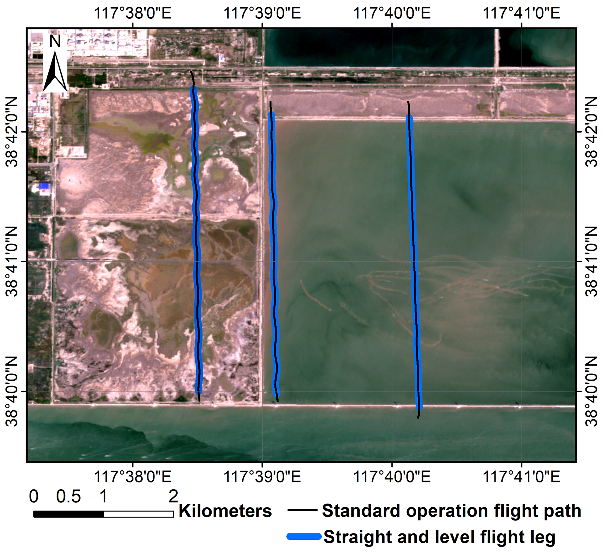
Figure 2 Flight trajectories of the standard operational flight campaign carried out between 8 and 16 August 2022 in the Binhai New Area, Tianjin, China. The land surface image is from the Sentinel-2A satellite image, with the true color combination acquired on 27 August 2022.

During the standard operational flight campaign, the atmospheric stability changed from stable (Monin–Obukhov stability parameter, $z/L=\mathrm{1.93}$) to very unstable ($z/L=-\mathrm{10.28}$) conditions as measured by the UAV, where z is the flight height above ground level, and L is the Obukhov length. The stable condition mostly occurred on the flight path located over the sea surface, while the unstable condition mostly occurred on the flight path located over the land surface. These flight data provided various measurement conditions for us to evaluate the performance of the developed UAV-based EC system.

2.3 Data processing

The raw data collected with the onboard data logger (CR6, Campbell, USA) are subsequently saved in the Network Common Data Form (NetCDF) format. These raw data include dynamic and static pressures, the attack and sideslip angles of incoming flow, slow (1 Hz) and fast (50 Hz) air temperatures, the mass concentrations of H₂O and CO₂, and the full navigation data (including 3D location, ground speed, angular velocity, and attitude, etc.) of the UAV. The subsequent data processing includes three stages in order to calculate the flux data from the measured raw data.

In the first stage, a moving-average filter was used to detect outliers in each variable. Detected outliers were removed and replaced by values obtained by linear interpolation. Outliers tend to be rare. However, if outliers constitute more than 20 % of the data points, the corresponding flight data should be discarded.

In the second stage, the georeferenced 3D wind vector is calculated. The full form of the equations for calculating the georeferenced wind vector with the UAV-based EC system is described in detail in the Supplement in Part A. From the airborne platform, the georeferenced wind vector is measured in two independent reference coordinate systems: the relative true airspeed (${\widehat{U}}_{\mathrm{a}}$) measurement in the aircraft coordinate system and the ground speed of the aircraft (U_p) in the georeferenced coordinate system. The georeferenced wind (U) is the vector sum of the relative true airspeed (${\widehat{U}}_{\mathrm{a}}$), the UAV's motion (U_p), and the tangential velocity due to the rotational motion of the aircraft (“lever arm” effect), which are described in Eq. (S2) in the Supplement. In this stage, the acquired calibration parameters (ϵ_ψ and ϵ_θ) from the calibration flight are substituted into the Eq. (S8) to correct the mounting angle offset errors between the 5HP and the CG of the UAV. The final equations for the georeferenced wind vector calculation (Eqs. S15–S17) revealed that the lever arm effects due to the spatial separation between the tip of the wind probe and the CG of the UAV may influence the wind measurements. Typically, the separation distance (L) is small, and the influence of the lever arm effects can be ignored when L is less than about 10 m (Lenschow, 1986). In the current UAV-based EC system, the displacements of the 5HP tip with respect to the CG of the UAV along the three axes of the UAV body coordinates are as follows: x^b=1.459 m, y^b=0 m, and z^b=0.173 m (in the Supplement in Part A). Therefore, in practice, the influence of leverage effects in georeferenced wind calculation was also ignored in this study. This was also confirmed by assessing the difference in the georeferenced wind vector with and without the leverage effect correction term in this study (in Sect. 3.1).

In the final stage, based on the EC technology and spatial averaging, turbulent fluxes are calculated using the covariances of vertical wind (w) with air temperature (T_a) for sensible heat flux (H), with water vapor density (q) for latent heat flux (LE), and with CO₂ density (c) for CO₂ flux (F_c) and with the necessary correction (Webb et al., 1980). The time lag due to the separation between the 5HP tip, the adjacent temperature probe, and the open-path gas analysis did not need to be corrected because the time delay was very small at the cruise airspeed of 30 m s⁻¹ and sensor separation of less than 20 cm. Only the measurement data from the straight-line portion of the flight path were used in the flux calculation. A detailed calculation procedure and formulas for calculating H, LE, and F_c used by the current UAV-based EC system are provided in the Supplement in Part B, including spatial averaging, coordinate rotation, and necessary correction (i.e., WPL correction for LE and F_c). In this study, all measured data of each straight and level flight leg (each with a length of about 4 km) from the standard operational flight campaign were used to calculate turbulent flux, regardless of the uncertainty in fluxes associated with spatial averaging.

2.4 Evaluation scheme

2.4.1 Wind measurement evaluation

The key to successful aircraft EC measurements lies in the translation of an accurately measured, aircraft-oriented wind vector to the georeferenced orthogonal wind vector (Thomas et al., 2012). Determining the georeferenced wind vector requires a sequence of thermodynamic and trigonometric equations (Metzger et al., 2012). These equations propagate various sources of error to the measured georeferenced wind vector. To estimate the measurement errors in the georeferenced wind vector, we used the linearized Taylor series expansions of Eqs. (S15)–(S17) derived by Enriquez and Friehe (1995) (Eqs. S18–S20) to determine the sensitivities of each of the georeferenced wind vector components with respect to the relevant variables. Then, these sensitivity terms can be combined to compute the overall measurement error (1σ) in the georeferenced 3D wind vector (Eqs. S21–S23).

The above wind measurement error analysis gives the nominal measurement precision of the georeferenced wind but does not consider the influence of environmental changes. Following the methods of Lenschow and Sun (2007), we assess the accuracy of wind measurements from the UAV in satisfying the minimum signal level needed for resolving the mesoscale variations in the three wind components in the encountered atmospheric conditions. Firstly, the minimum required signal level for measurement of vertical airspeed (ω) under the encountered atmospheric conditions could be estimated as (Lenschow and Sun, 2007)

$$\begin{array}{}\text{(1)}& {\displaystyle \frac{\partial w}{\partial t}}<\mathrm{0.2}\sqrt{\mathrm{2}}{\mathit{\sigma }}_w\mathrm{2}\mathit{\pi }k{U}_{\mathrm{a}},\end{array}$$

where the true airspeed (U_a) is set to a mean cruise speed of 30 m s⁻¹, σ_w is the peak signal magnitude of the power spectra, and k is the corresponding wavenumber (Thomas et al., 2012). The measurement error in the vertical wind component can be calculated as (Lenschow and Sun, 2007)

$$\begin{array}{}\text{(2)}& {\displaystyle \frac{\partial w}{\partial t}}\cong \mathrm{\Theta }{\displaystyle \frac{\partial U_{\mathrm{a}}}{\partial t}}+U_{\mathrm{a}}{\displaystyle \frac{\partial \mathrm{\Theta }}{\partial t}}+{\displaystyle \frac{\partial w_{\text{UAV}}}{\partial t}},\end{array}$$

with $\mathrm{\Theta }=\mathit{\alpha }-\mathit{\theta }$, where α is the attack angle, θ is the pitch angle, and w_UAV is the UAV's vertical velocity. According to Lenschow and Sun (2007), the signal level and mesoscale fluctuation of horizontal wind components (u and v) are considerably larger than those of vertical wind, so the accuracy criteria are not nearly as stringent. The measurement error of the horizontal wind component could be calculated as (Lenschow and Sun, 2007)

$$\begin{array}{}\text{(3)}& {\displaystyle \frac{\partial u}{\partial t}}\cong -{\displaystyle \frac{\partial U_{\mathrm{a}}}{\partial t}}+{\displaystyle \frac{\partial u_{\text{UAV}}}{\partial t}},\text{(4)}& {\displaystyle \frac{\partial v}{\partial t}}\cong \mathrm{\Psi }{\displaystyle \frac{\partial U_{\mathrm{a}}}{\partial t}}+v_{\text{tas}}{\displaystyle \frac{\partial \mathrm{\Psi }}{\partial t}}+{\displaystyle \frac{\partial v_{\text{UAV}}}{\partial t}},\end{array}$$

and

$$\begin{array}{}\text{(5)}& \mathrm{\Psi }\equiv {\mathit{\psi }}^{\prime }+\mathit{\beta },\end{array}$$

where u_UAV and v_UAV are the UAV's horizontal velocity measured from INS, ψ^′ is the departure of the measured true heading from the average true heading, and β is the sideslip angle of airflow. If the measurement error of the 3D wind vector from Eqs. (2)–(4) is smaller than the required minimum signal level of the vertical and horizontal wind components, it can be confirmed that the measurement accuracy of the georeferenced 3D wind vector from the UAV is sufficient to resolve the mesoscale variations in the three wind components in the encountered atmospheric conditions.

In addition, accurate measurements of the georeferenced wind vector typically not only depend on the measurement precision of the sensors (i.e., 5HP and INS), but also relate to the quality of the calibration parameters and the geometry structure of the UAV (i.e., flow distortion and leverage effect). To evaluate the effect of the latter two, a calibration flight campaign (Sect. 2.2.1) was performed to determine the calibration parameter (ϵ_ψ, ϵ_θ) and check its quality, as well as ascertain the effects of the lever arm and upwash by the wings. The methods for acquiring the calibration parameter were given by Vellinga et al. (2013) and Sun et al. (2021a), and the results are reported in the Supplement in Part C (Figs. S2 and S3). During the in-flight calibration campaign, a racetrack maneuver was performed to check the quality of the calibration parameters determined from the box flight maneuver. The initial (${\mathit{ϵ}}_{\mathit{\psi }}=\mathrm{0}{}^{\circ }$, ${\mathit{ϵ}}_{\mathit{\theta }}=\mathrm{0}{}^{\circ }$) and calibrated (${\mathit{ϵ}}_{\mathit{\theta }}=-\mathrm{0.183}{}^{\circ }$, ${\mathit{ϵ}}_{\mathit{\psi }}=\mathrm{2}{}^{\circ }$, in the Supplement in Part C) sets of parameters were used to calculate the georeferenced wind vector. By comparing the mean and standard deviation (SD) of the horizontal and vertical wind vectors between the initial and calibrated sets, the quality of the georeferenced wind vector measurement in real environmental conditions can be verified.

The relative wind vector (${\widehat{U}}_{\mathrm{a}}$) measured by the aircraft is susceptible to flow distortion because the airplane must distort the flow to generate lift and thrust. The aircraft's propellers, fuselage, and wings are the main sources of flow distortion as flow barriers (Metzger et al., 2011). For fixed-wing aircraft, the wind probe, mounted on the nose of the UAV and extended as far forward off the fuselage as possible, could avoid the flow distortion induced by the fuselage and propellers. The effects from the induced upwash by the wings can also influence the correspondence between the measured and free-stream flow variables (Garman et al., 2008). The induced upwash modifies the local angle of attack, causing the measured attack angle (α) to be larger than the free-stream attack angle (α_∞) (Garman et al.,  2008). Therefore, for wind measurements by large-scale occupied fixed-wing aircraft, the upwash effects must be corrected (Garman et al., 2008; Kalogiros and Wang, 2002). However, the UAV seldom needs this correction due to the size of the fuselage and the fact that the airspeed is very low compared to an occupied aircraft.

In this study, in order to assess whether the lift-induced upwash can be safely ignored by the current UAV-based EC system, an acceleration–deceleration flight maneuver was performed. According to Crawford et al. (1996), the pitch angle (θ) of the INS instrument can be utilized as an estimate of the free-stream attack angle (α_∞) if the aircraft's vertical velocity is 0, since it is unaffected by lift-induced upwash and varies directly with α_∞ when the ambient vertical wind is 0. Under ideal conditions (0 aircraft vertical velocity and 0 ambient vertical wind), the approximation relationship of θ≅α_∞ is valid when $\mathit{\theta }<\mathrm{6}{}^{\circ }$ (Crawford et al., 1996; Vellinga et al., 2013). Departures from the 1:1 relationship can be caused by airflow distortion around the airplane behind the 5HP. The acceleration–deceleration maneuver produced various pitch and attack angles measured under various airspeeds, which allowed a direct comparison between the pitch angle (θ) and the attack angle (α). If the slope between α and θ is close to unity, it indicates that the influence of lift-induced upwash can be ignored; otherwise, its influence should be corrected (Garman et al., 2006). Meanwhile, the influence of leverage effects was also evaluated based on the measurement data from the acceleration–deceleration maneuver by considering or ignoring the leverage effect correction term in Eqs. (S15)–(S17).

2.4.2 Flux measurement error caused by instrumental noise

Flux measurement errors from UAVs can be attributed to several sources, mainly including instrumental noise, data handling, atmospheric conditions, spatial averaging length, and bumpy flight environments (Mahrt, 1998; Finkelstein and Sims, 2001; Mauder et al., 2013). They can be systematic or random. Determination of the flux measurement error caused by instrument noise is very useful, as it is related not only to the system performance, but also to the minimum resolvable capability for the flux to be measured. In the current study, uncertainty related to instrumental noise (listed in Table 1) was estimated using the direct method proposed by Billesbach (2011). This method is called “random shuffle” (denoted as RS) and was “designed to only be sensitive to random instrument noise”. According to Billesbach (2011), the uncertainty in the flux covariance can be expressed as

$$\begin{array}{}\text{(6)}& {\mathit{\sigma }}_{\stackrel{\mathrm{‾}}{w^{\prime }{x}^{\prime }}}={\displaystyle \frac{\mathrm{1}}{N}}{\sum }_{i,j=\mathrm{1}}^N{w}^{\prime }\left(t_i\right)x^{\prime }\left(t_j\right),\end{array}$$

where x is the target entity of the covariance, and N is the number of measurements contained in the block averaging period, j∈[1…N], but the values are in a random order. The idea behind the RS method was that the random shuffling would remove the covariance between biophysical (source or sink) and transport mechanisms, leaving only the random “accidental” correlations mostly attributed to instrument noise (Billesbach, 2011). It means that the shuffled component x is uncorrelated to itself in time or space and decorrelates x from w, resulting in two independent variables (i.e., $\stackrel{\mathrm{‾}}{w^{\prime }{x}^{\prime }}\sim \mathrm{0}$), and any residual value (i.e., $\stackrel{\mathrm{‾}}{w^{\prime }{x}^{\prime }}\ne \mathrm{0}$) of the covariance is attributed to random instrument noise.

In this study, in order to obtain a robust estimate of the instrumental noise, ${\mathit{\sigma }}_{\stackrel{\mathrm{‾}}{w^{\prime }{x}^{\prime }}}$ was repeatedly calculated 20 times for every straight and level flight leg in the operational flight (Fig. 2), and the means of the absolute values of these repeated estimated ${\mathit{\sigma }}_{\stackrel{\mathrm{‾}}{w^{\prime }{x}^{\prime }}}$ values were used to estimate the random uncertainty related to instrumental noise. According to Rannik et al. (2016), the RS method tends to overestimate the covariance uncertainty. Then, the uncertainties in the flux covariance of sensible heat $\left({\mathit{\sigma }}_{\stackrel{\mathrm{‾}}{w^{\prime }{T}^{\prime }}}\right)$, latent heat (${\mathit{\sigma }}_{\stackrel{\mathrm{‾}}{w^{\prime }{\mathit{\rho }}_{\mathrm{v}}^{\prime }}}$), and CO₂ (${\mathit{\sigma }}_{\stackrel{\mathrm{‾}}{w^{\prime }{\mathit{\rho }}_{\mathrm{c}}^{\prime }}}$) were estimated using the RS method.

It should be noted that the measurement error in the EC flux is influenced not only by the uncertainty in the raw covariance but also by the propagated errors form the correction terms (i.e., WPL correction) or any lens contamination (Serrano-Ortiz et al., 2008). The signal quality of the IRGA was checked before each flight measurement to ensure that the measurement of gas concentrations is not affected by lens contamination. The relative uncertainty in the flux measurement was estimated using the partial derivatives of the flux calculation equation derived by Liu et al. (2006) (Eqs. S28–S30). These equations ignored the perturbation terms from the errors in the individual scalar (i.e., ρ_v, ρ_c, T), which were proved to be very small (Serrano-Ortiz et al., 2008). At last, after several repetitive calculations of Eq. (6), the averaged uncertainty results were then combined to Eqs. (S28)–(S30) to estimate the flux measurement error caused by instrumental noise.

2.4.3 Resonance effects

Previous work has found that the measurement of the atmospheric scalars (e.g., air temperature as well as H₂O and CO₂ concentrations) by the current UAV-based EC system was susceptible to resonance effects caused by the operation of the engine and propeller (Sun et al., 2021b). In order to further reduce the noise influence from resonance effects, the vibration damping structure was further optimized. The reference (co)spectral curve of Massman and Clement (2005) was then used to quantify the influence of the resonance effects remaining after vibration isolation optimization. Massman and Clement (2005) gave the generalization mathematical expression of the models of spectra and cospectra as follows:

$$\begin{array}{}\text{(7)}& \text{Co}\left(f\right)=A_{\mathrm{0}}{\displaystyle \frac{\mathrm{1}/f_x}{[\mathrm{1}+m(f/f_x{)}^{\mathrm{2}\mathit{\mu }}{]}^{\frac{\mathrm{1}}{\mathrm{2}\mathit{\mu }}\left(\frac{m+\mathrm{1}}{m}\right)}}},\end{array}$$

where f is frequency (Hz), f_x is the frequency at which fCo(f) reaches its maximum value, A₀ is a normalization parameter, m is the (inertial subrange) slope parameter, and μ is the broadness parameter. To describe cospectra, m should be $\mathrm{3}/\mathrm{4}$; to describe spectra, m should be $\mathrm{3}/\mathrm{2}$. According to Massman and Clement (2005), μ was set to $\mathrm{7}/\mathrm{6}$ under stable atmospheric conditions and to $\mathrm{1}/\mathrm{2}$ under unstable atmospheric conditions. The fast Fourier transform (FFT) method was used to calculate the spectra and cospectra of the measured turbulent variables. Before calculating the turbulence (co)spectra, conditioning of the raw turbulence data was performed, including linear detrending and tapering using the Hamming window to reduce the spectral leakage (sharp edge) according to Kaimal et al. (1989).

The noise influence from resonance mainly appears in the high-frequency domain. According to the feature of the spectral curve, the frequency range of the noise region was artificially designated to f>8 Hz for air temperature, f=1–5 Hz for water vapor, and f=1–8 Hz for CO₂. The normalized spectral and cospectral curves were adopted, and the area difference in the designated frequency range beneath the (co)spectral curve between the measured and reference (co)spectral curves was calculated to quantify the influence of resonance noise in the variance and flux covariance of the measured atmospheric scalars. An example is shown in Fig. 3, and also shown is the reference (co)spectral curve of Massman and Clement (2005), with the (co)spectral maximum at f_x=0.1. The red region in Fig. 3 represents the extent of the impact of the resonance noise in the variance (Fig. 3a–c) and flux covariance (Fig. 3d–f) of the measured scalars.

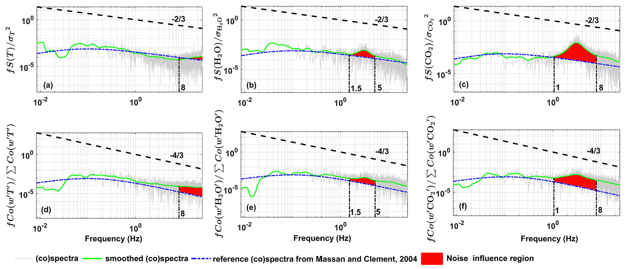
Figure 3 Influence of the resonance noise on the spectral (a–c) and cospectral (d–f) curves of the measured scalars based on the measured data from one standard operational flight carried out on 8 August 2022 in the Binhai New Area, Tianjin, China. The red region is the area difference in the designated frequency range (vertical dashed–dotted black line) beneath the (co)spectral curve between the measured and reference (co)spectral curve.

2.4.4 Sensitivity analysis

To understand the relevance of the calibration parameters for the measurement of the georeferenced wind vector and turbulent flux, two sensitivity tests were conducted. The magnitude of the perturbation in the wind vector and turbulent flux was investigated as a function of the uncertainties in the four calibration parameters, including three mounting misalignment angles (ϵ_ψ, ϵ_θ, ϵ_ϕ) between the 5HP and the CG of the UAV and one temperature recover factor (ϵ_r=0.82) used to calculate the ambient temperature (Eq. 3 in Sun et al., 2021a).

First, the sensitivity of the georeferenced wind vector and turbulent flux to the uncertainties in the individual calibration parameters was investigated. The georeferenced wind vector and turbulent flux were calculated based on the straight leg (about 4 km) of the standard operational flight by adding an error of ±30 % to the calibrated value of each calibration parameter alternately, except for ϵ_ϕ, for which the typical range of ±0.9^∘ was taken for sensitivity analysis (Vellinga et al., 2013).

Then, in order to test the overall interaction between the parameters, a second sensitivity test was performed to calculate the georeferenced wind vector and turbulent fluxes by adding a ±30 % error to all calibration parameters simultaneously. Lastly, relative errors (REs) were calculated to evaluate the perturbation in the wind vector and turbulent flux under the variation in each calibration parameter as well as under simultaneous variation in all calibration parameters. In the sensitivity analysis, the calculated georeferenced wind and turbulent flux, whose absolute values were less than their least-resolvable magnitude, were filtered out to avoid the influence of the errors contained in the measurements themselves on the results.

2.4.5 Relative error

In this study, relative error (RE) was used to evaluate the influence of different factors on the measurements of the georeferenced wind vector and turbulent flux. It is defined as

$$\begin{array}{}\text{(8)}& \text{RE}={\displaystyle \frac{\left|x_{\mathrm{0}}\right|-\left|x\right|}{\left|x\right|}}\times \mathrm{100}\mathit{\%},\end{array}$$

where $\left|\right|$ means the absolute value, x is the “true” value, and x₀ is the influenced value. RE>0 means the exerted influence will cause the measurement value to be larger than the true value and vice versa.

3 Results

3.1 Wind measurement evaluation

Wind measurement evaluation for the UAV-based EC system includes three aspects: (1) checking measurement precision and the system's ability to resolve the mesoscale variations in the wind, (2) checking the quality of the acquired calibration parameters, and (3) checking whether the measured wind vector is affected by upwash flow and leverage effects.

First, according to the equations described in the Supplement in Part A (Eqs. S18–S23), the measurement precision of the horizontal wind components is a function of the true airspeed and true heading, while the measurement precision of vertical wind components is largely decided by the true airspeed. The typical values of the true airspeed, ranging from 25 to 35 m s⁻¹ (interval of 1 m s⁻¹), and the true heading, ranging from 0 to 180^∘ (interval of 30^∘), were used in the evaluation of the wind measurement error. The measurement precision (1σ) of the georeference 3D wind vector from aircraft was then estimated using the measurement precision of the related parameters from Table 1. The results are shown in Fig. 4 for the measurement precision of horizontal wind (σ_u and σ_v in Fig. 4a and b) and vertical wind (σ_w in Fig. 4c). The typical values of the measurement precision range from 0.05 to 0.07 m s⁻¹ for the horizontal wind component u, from 0.02 to 0.08 m s⁻¹ for the horizontal wind component v, and from 0.05 to 0.07 m s⁻¹ for the vertical wind component w.

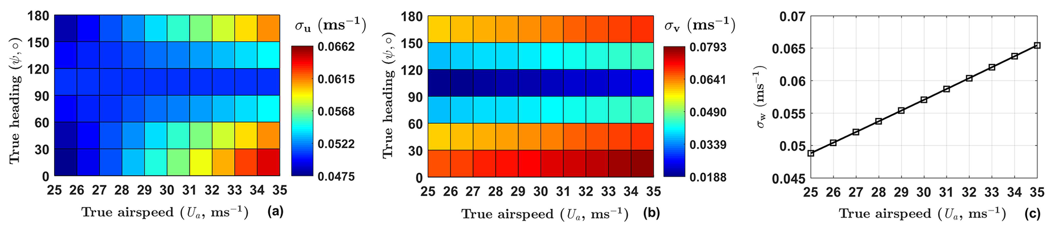
Figure 4 Estimated measurement precision (1σ) of the horizontal wind (a, b) and vertical wind (c) according to the equations described in the Supplement in Part A (Eqs. S18–S23).

Generally speaking, an autopiloted UAV can maintain a near-constant true airspeed during the cruise flight phase. At a true airspeed of 30 m s⁻¹ for the current UAV during the cruising, the maximum measurement errors in the northward, eastward, and vertical velocities of the georeferenced wind components were calculated as approximately 0.06, 0.07, and 0.06 m s⁻¹, respectively. Then, we assume that a minimum signal-to-noise ratio of 10:1 is required to measure the wind components with sufficient precision for EC measurement (Metzger et al., 2012). Accordingly, in the real environments, horizontal and vertical wind speeds greater than 0.7 and 0.6 m s⁻¹, respectively, can be reliably measured (Table 2).

Table 2 The maximum measurement error in the northward (u), eastward (v), and vertical (w) velocities of the georeferenced wind components at the true airspeed of 30 m s⁻¹ and the least-resolvable magnitude assuming the minimum required signal-to-noise ratio of 10:1.

The above results gave the nominal precision for wind measurement that does not consider the influence of environmental conditions. Changes in the environment will lead to sensor drift, increasingly deteriorating the measurement with flight duration (Metzger et al., 2012; Lenschow and Sun, 2007). Following the methods of Lenschow and Sun (2007), the ability of wind measurements from UAVs to resolve the mesoscale variations in the 3D wind components in the encountered atmospheric conditions was assessed. For the vertical wind, the mesoscale variability was defined as the peak signal magnitude of the power spectral curve. The corresponding average wavenumber was determined as 0.09 m⁻¹ based on the straight flight leg (about 4 km, lasting about 120 s) of the standard operational flight. Then, according to Eq. (1), the minimum required signal level for the vertical wind measurement was estimated as $\partial w/\partial t\simeq \mathrm{0.14}$ m s⁻². The accuracy of the vertical wind measurement using Eq. (2) is estimated as follows. The first term on the right-hand side of Eq. (2) is dominated by the drift in the differential pressure transducer; the value of $\partial U_{\mathrm{a}}=\mathrm{0.05}$ m s⁻¹ acquired from the wind tunnel test was used (Table 1). The histogram of Θ derived from the standard operational flights is shown in Fig. 5. The 99 % confidence interval indicates that the value of Θ seldom exceeds ±3^∘, i.e., ±0.053 radians. Thus, the value of the first term was estimated as $\mathrm{2.2}\times {\mathrm{10}}^{-\mathrm{5}}$ m s⁻².

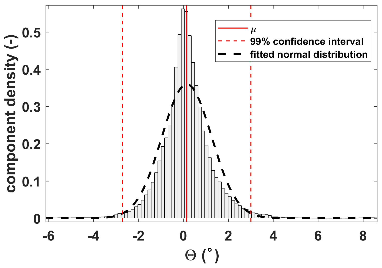
Figure 5 Histogram of Θ derived from the standard operational flights. The component density is scaled so that the histogram has a total area of 1. The red vertical lines indicate the distribution average (solid) and the 99 % confidence interval (dashed). The dashed black bell curve displays a reference fitted normal distribution.

The second term in Eq. (2) is a combination of the INS pitch accuracy and 5HP attack angle accuracy. The combined accuracy of these two sensors was applied to derive $\partial \mathrm{\Theta }=\mathrm{0.0024}$ radians. Thus, the second term in Eq. (2) was estimated as $\mathrm{6}\times {\mathrm{10}}^{-\mathrm{4}}$ m s⁻². Finally, the third term in Eq. (2) was estimated as $\mathrm{1.7}\times {\mathrm{10}}^{-\mathrm{4}}$ m s⁻², according to the stated accuracy of the vertical velocity from the INS. The overall performance of the vertical wind measurement ($\mathrm{7.9}\times {\mathrm{10}}^{-\mathrm{4}}$ m s⁻²) was accurate enough to resolve the mesoscale variations in vertical air velocity.

The required accuracy of horizontal wind for mesoscale measurement was estimated to be 10 times larger than that of vertical wind; i.e., $\partial u/\partial t\simeq \partial v/\partial t\simeq \mathrm{1.4}$ m s⁻². The measurement accuracy of the horizontal wind component u was estimated as $\mathrm{4.8}\times {\mathrm{10}}^{-\mathrm{4}}$ m s⁻² according to Eq. (3). Like the first term in Eq. (2), with the value of Ψ rarely exceeding ±0.18 radians, the measurement accuracy of the horizontal wind component v was estimated as $\mathrm{2.7}\times {\mathrm{10}}^{-\mathrm{2}}$ m s⁻² according to Eq. (4). Thus, the measurement accuracy of the horizontal wind components was accurate enough to resolve the mesoscale variations in the horizontal air velocity as well.

Second, before checking the quality of the acquired calibration parameters, the calibration results of the offset in pitch (ϵ_θ) and heading (ϵ_ψ) angles based on the box maneuver are provided in the Supplement in Part C (Figs. S2 and S3). The final calibration values are ${\mathit{ϵ}}_{\mathit{\theta }}=-\mathrm{0.183}$^∘ and ϵ_ψ=2^∘. In order to verify the quality of these calibration parameters, a racetrack maneuver was performed. Figure 6 shows the validation results by plotting wind vector statistics and calculating summary statistics for the racetrack maneuver (including turns), using the initial (${\mathit{ϵ}}_{\mathit{\theta }}={\mathit{ϵ}}_{\mathit{\psi }}=\mathrm{0}$^∘, Fig. 6a) and calibrated (Fig. 6b) sets of parameters, respectively. Introduction of the calibration parameter effectively improved the quality of the georeferenced wind vector measurement. The SD for wind direction, ${\mathit{\sigma }}_{U_{\text{dir}}}$, is 4.9^∘ for the calibrated set compared to 8.7^∘ for the initial set, and the SD of wind speed, σ_U, is 0.52 m s⁻¹ for the calibrated set compared to 1.12 m s⁻¹ for the initial set. The averaged vertical wind speed is much closer to 0 ($\stackrel{\mathrm{‾}}{w}=-\mathrm{0.006}$ m s⁻¹) for the calibrated set than for the initial set ($\stackrel{\mathrm{‾}}{w}=\mathrm{0.1}$ m s⁻¹). For the horizontal wind, it is evident from Fig. 6 that the measurement of wind direction and velocity is insignificantly affected by sharp turns. On the contrary, the measurement of the vertical wind component is obviously affected by turns in flight, as shown by the large fluctuations in the vertical wind speed around the scan value of 150 (bottom panels in Fig. 6). It should be noted that the influence of upwash flow and the leverage effect are not considered in the calculated georeferenced wind vector.

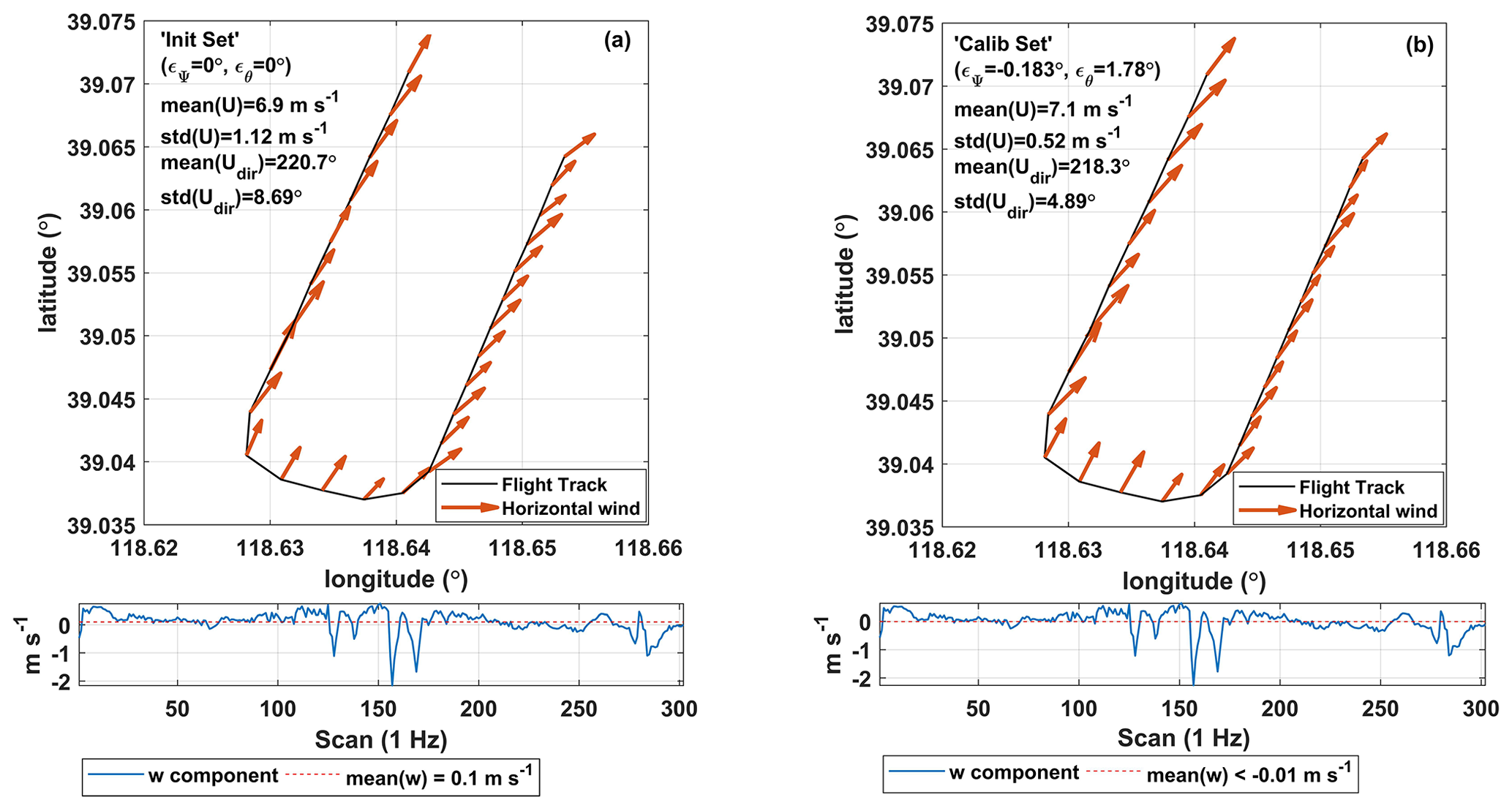
Figure 6 Quality check of the calibration parameter by plotting wind vector statistics and calculating summary statistics for the racetrack maneuver, using the initial (a) and calibrated (b) sets of parameters, respectively. The calibration flight was carried out on 4 September 2022 at the Caofeidian shoal harbor in the Bohai Sea of northern China.

Third, in order to check the influence of the lift-induced upwash on the measured attack angle from the 5HP, an acceleration–deceleration flight maneuver was performed. During the acceleration–deceleration maneuver, INS data showed the vertical velocity of the UAV to be 0.05±0.2 m s⁻¹, the altitude of the UAV to be 392±0.6 m, and the heading of the UAV to be 199±2.4^∘. We assume that the flight conditions meet the requirements of the acceleration–deceleration maneuver (Vellinga et al., 2013). The relationship between the pitch angle (θ) measured by the INS and the attack angle (α) measured by the 5HP is plotted in Fig. 7, where the attack angle was not corrected for lift-induced upwash. The slope (0.94) between θ and α is close to its theoretical value of 1, and the intercept (0.16) is close to 0. It indicates that the lift-induced upwash has only a very small effect on the attack angle, and the influence of upwash could be ignored.

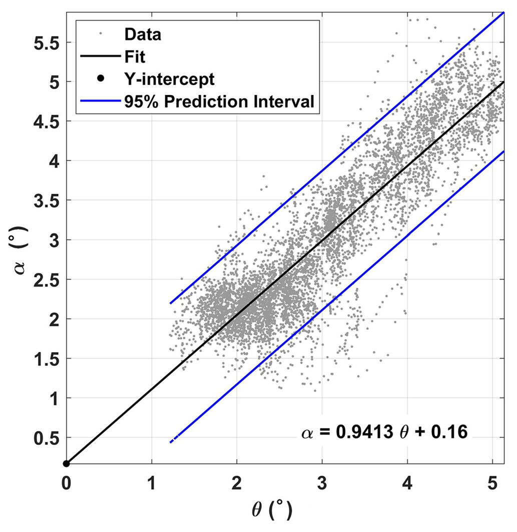
Figure 7 Relationship between the pitch angle (θ) measured by the integrated navigation system (INS) and the attack angle (α) measured by the five-hole probe (5HP). The fitted linear equation is also shown.

Finally, the georeferenced wind vector was calculated with and without the correction for the leverage effect based on the measurement data from the acceleration–deceleration flight maneuver. The averaged relative differences between the corrected and uncorrected horizontal and vertical wind speeds are 0.1 % and 0.2 %, respectively. The SD for horizontal wind speed is 0.307 m s⁻¹ without the level arm term compared to 0.306 m s⁻¹ when the level arm term is introduced. The SD of vertical wind speed is 0.254 m s⁻¹ without the level arm term compared to 0.253 m s⁻¹ with the level arm term. The correction of the leverage effect had a minimal effect on improving the georeferenced wind vector measurement; therefore, this correction term can be ignored.

3.2 Flux measurement error caused by instrumental noise

Flux measurement error caused by the instrumental noise gives the lowest limit of the value that the UAV-based EC system is able to measure. It was assessed by combining the covariance uncertainty estimated by the RS method and the propagation of errors in the flux correction terms. Before estimating the flux covariance uncertainty with the RS method, using the measured data from each straight and level flight leg of the standard operational flight (Fig. 2), the normalized integrated cospectral (ogives) curves of sensible heat (Fig. 8a), latent heat (Fig. 8b), and CO₂ (Fig. 8c) flux are formed as a function of the wavenumber (k), where $k=\mathrm{2}\mathit{\pi }f/U_{\mathrm{a}}$. As shown in Fig. 8, although the heterogeneous turbulence (or mesoscale turbulence) interfered with the shape of the ogive curves, most curves converged at the high- and low-frequency ends, which indicated that these segmented data were sufficiently long to represent the lowest significant frequencies contributing to the covariance (Sun et al., 2018).

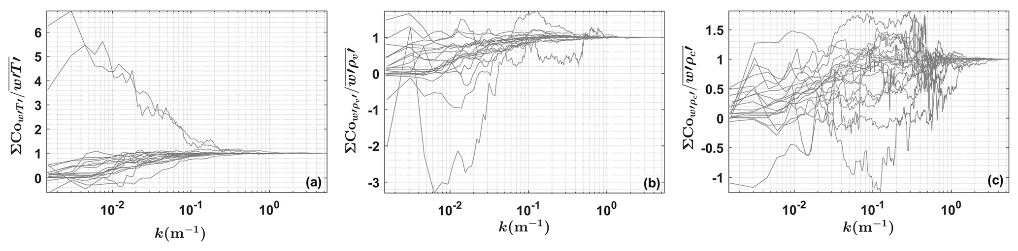
Figure 8 Normalized ogive curves as a function of the wavenumber for the flux covariance of sensible heat (a), latent heat (b), and CO₂ (c) from each straight and level flight leg of the standard operational flights in Sect. 2.2.2.

The results of the instrumental-noise-related relative flux measurement error compared to the magnitude of the flux are shown in Fig. 9. It can be seen that the flux measurement error caused by instrumental noise significantly decreases when the flux magnitude increases. It is not surprising, since, in theory, instrumental noise is usually close to a constant, and the relative flux measurement error caused by instrumental noise will decrease with increasing measurement magnitude. Overall, instrumental noise has the least effect on latent heat flux (ranging from 0.02 % to 2.42 % in this study) measurements, followed by sensible heat flux (ranging from 0.05 % to 8.6 % in this study), and has the greatest effect on the measurement of the CO₂ flux (ranging from 0.22 % to 75.6 % in this study). Then, a simple rational function relationship between the relative measurement error and the flux magnitude is fitted according to the measured data, where the constant term in the denominator is set to 0. The fitted coefficient in the numerator can be considered to be the flux measurement error caused by instrumental noises, which are 0.03 $\mathrm{\mu }\mathrm{mol}{\mathrm{m}}^{-\mathrm{2}}{\mathrm{s}}^{-\mathrm{1}}$, 0.02 W m⁻², and 0.08 W m⁻² for the measurement of the CO₂ flux, sensible heat flux, and latent heat flux, respectively. At last, using the signal-to-noise ratio of 10:1, the minimum magnitudes for reliably resolving the CO₂ flux as well as sensible and latent heat fluxes were estimated as 0.3 $\mathrm{\mu }\mathrm{mol}{\mathrm{m}}^{-\mathrm{2}}{\mathrm{s}}^{-\mathrm{1}}$, 0.2 W m⁻², and 0.8 W m⁻², respectively.

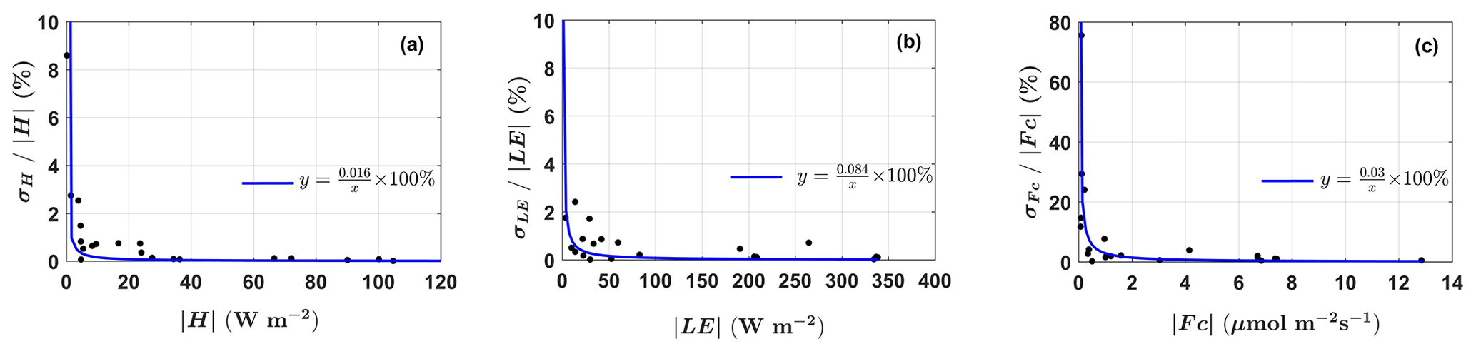
Figure 9 Relative flux measurement error caused by the instrumental noise plotted against the magnitude of the flux. Also shown is the fitted error curves. Measured data were from the standard operational flights in Sect. 2.2.2.

3.3 Resonance noise

The resonance noise from the engine and propeller can lead to systematic overestimation of the variance and covariance of the observed atmospheric scalars. The noise mainly appears in the high-frequency domain of the (co)spectra, and the reference (co)spectral curve of Massman and Clement (2005) was used to quantify the systematic bias caused by the resonance noise.

All spectral curves of the variance of the measured scalars (including air temperature as well as H₂O and CO₂ concentrations) approximately followed the reference spectral curve and the reference $-\mathrm{2}/\mathrm{3}$ slope in the inertial subrange (Fig. 3a–c). The largest scatter occurred in the spectra of CO₂ (Fig. 3c). When comparing the spectral curve with the reference spectra, the resonance noise led to a systematic deviation in the variance of the air temperature as well as H₂O and CO₂ concentrations of 0.1±0.1 %, 1.0±0.79 %, and 4.4±0.66 %, respectively. For the flux covariance of sensible heat, latent heat, and CO₂, all the cospectral curves approximately follow the reference cospectral curve and the reference $-\mathrm{4}/\mathrm{3}$ slope in the inertial subrange (Fig. 3d–f). Compared with the reference cospectra, the resonance noise led to a systematic deviation in the flux of sensible heat, latent heat, and CO₂ of 0.07±0.004 %, 0.3±0.25 %, and 2.9±1.62 %, respectively.

The results show that the resonance noise has a very little impact on the measured variance and flux covariance. The measurements of the CO₂ concentration and flux are the most susceptible to the resonance noise, but the impact of this noise is limited to around 5 % of the observed value.

3.4 Sensitivity analysis

In order to investigate the relevance of the calibration parameters for the measurement of the georeferenced wind vector and turbulent flux, two sensitivity tests were conducted by adding an error of ±30 % to the calibrated parameters used (ϵ_ψ, ϵ_θ, ϵ_ϕ,ϵ_r). We assumed that the maximum uncertainties contained in the calibration parameter are not more than 30 % of its own value.

First, the sensitivity of the georeferenced 3D wind and turbulent flux to the uncertainty in the individual calibration parameter was tested. The RE value is used to quantify the sensitivity, and the results are summarized in Tables 3 and 4. For the measurement of the georeferenced wind vector, Table 3 shows that the uncertainties in the temperature recovery factor (ε_r) and 5HP mounting misalignment error in the roll (ϵ_ϕ) angle do not contribute significantly to errors in the wind measurements, which were typically smaller than 4 % of the observed value in this study. Parameter ε_θ had the largest effect on the vertical wind component (up to 30 %), whereas ε_ψ had the largest effect on the horizontal wind component. For the measurement of turbulent fluxes, Table 4 shows that the errors in ε_r and ϵ_ϕ, which were typically smaller than 5 % of the observed value in this study, do not significantly influence the flux measurements. Uncertainties in the ε_θ and ε_ψ calibration parameters had significant effects on the measurement of turbulent fluxes. Errors in ε_θ result in significant perturbation (large RE variance) in the measured turbulent fluxes, including sensible heat, latent heat, and CO₂, while errors in ε_ψ to some extent mainly affect the measurement of the latent heat flux (RE may affect the latent heat flux with up to 15 %).

Table 3 RE from the sensitivity test for the georeferenced 3D wind vector ($u,v,w$). An error factor of ±30 % was added to each calibrated parameter. The georeferenced 3D wind vector was calculated based on the straight leg of the standard operational flight.

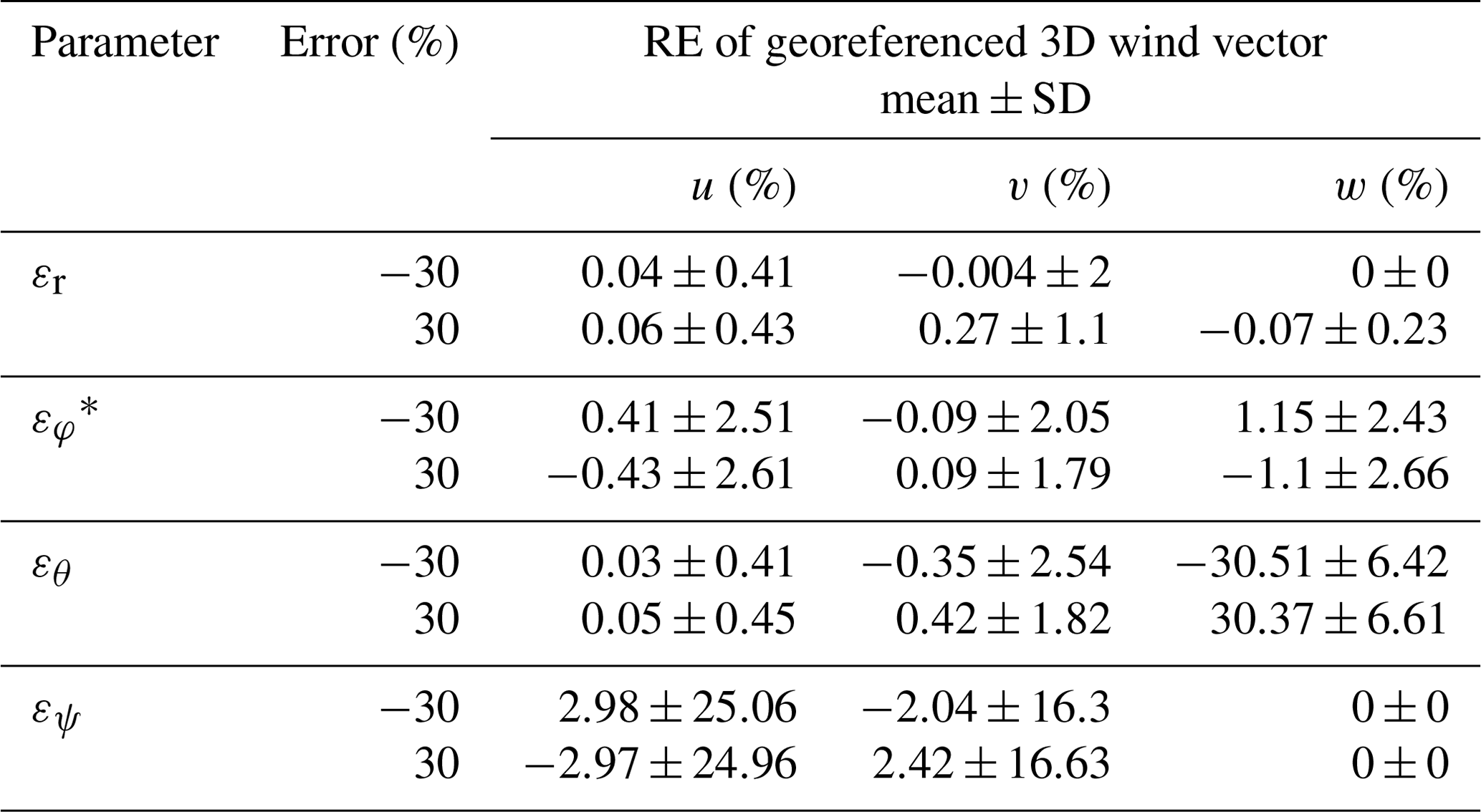
^∗ The optimum calibration value is set to 0; ε_φ is varied over $\pm \mathrm{0.9}{}^{\circ }$, which is 30 % of its typical range.

Table 4 RE from the sensitivity test for the turbulent fluxes. An error factor of ±30 % was added to each calibrated parameter. The turbulent fluxes were calculated based on the straight leg of the standard operational flight.

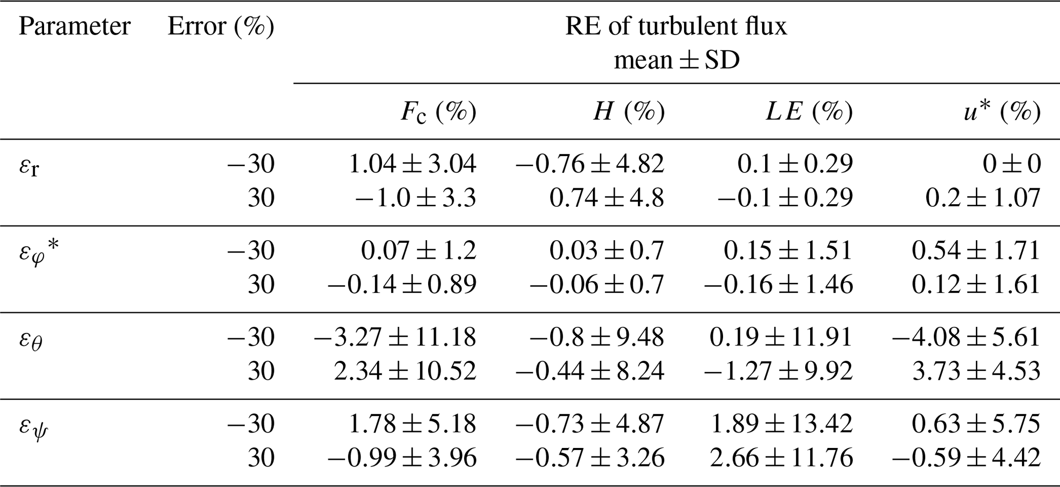
^∗ See Table 3.

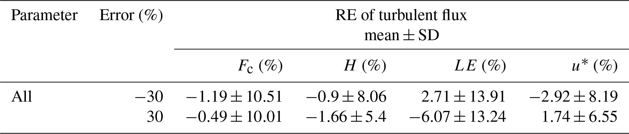
The second sensitivity test was performed to evaluate the overall interaction between the calibration parameters and the calculation of the georeferenced wind vector and turbulent flux by adding an error of ±30 % to all the calibration members simultaneously. Tables 5 and 6 provide a summary of the RE from the second sensitivity test. For the measurement of the georeferenced wind vector (Table 5), adding an error of ±30 % to all the calibration parameters at the same time resulted in great perturbations in both the horizontal (low RE with high variance) and vertical wind components (high RE with low variance). For the measurement of turbulent fluxes, adding a 30 % error in all of the calibration parameters can result in errors in the measured fluxes of more than 10 %. In addition, Table 6 also reveals that the latent heat flux is more sensitive to the errors in the calibration parameter than other measured fluxes (higher mean and variance of the RE compared to other measurements).

Table 5 RE from the sensitivity test for the georeferenced 3D wind vector ($u,v,w$) calculated by adding an error of ±30 % to all the calibrated parameters simultaneously. The georeferenced 3D wind vector was calculated based on the straight leg of the standard operational flight.

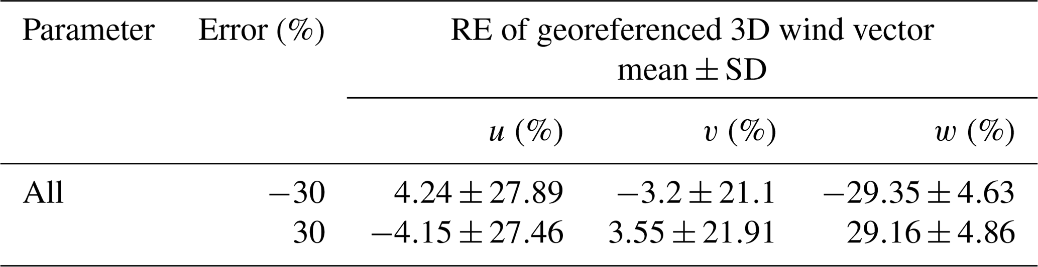
Table 6 RE from the sensitivity test for the turbulent flux calculated by adding an error of ±30 % to all the calibrated parameters simultaneously. The turbulent flux was calculated based on the straight flight leg of the standard operational flight.

4 Discussions

The current study aimed to evaluate the performance of the UAV-based EC system developed by Sun et al. (2021a) in the measurements of wind vector and turbulent fluxes.

First, the wind measurement precision (nominal precision) of the UAV-based EC system was estimated by propagating the sensor errors to the georeferenced wind vector using the linearized Taylor series expansions from Enriquez and Friehe (1995). The 1σ precision for the georeferenced wind measurement was estimated to be ±0.07 m s⁻¹, and the least-resolvable magnitude for wind measurement was estimated to be 0.7 m s⁻¹ by assuming the minimum signal-to-noise ratio of 10:1. The derived wind measurement minimum resolvable magnitude can be used as a basic reference for the wind measurement capability of the UAV-based EC system, and the measured values of wind vectors smaller than the minimum resolvable values should be considered unreliable. The accuracy of the sensors was also assessed by examining the collected data in the real environment. Our results revealed that the overall performance of the georeferenced wind measurement is of sufficient accuracy to resolve the mesoscale variations in the 3D wind components under the encountered atmospheric conditions. Therefore, it is possible to capture the mesoscale variability in the atmospheric boundary layer (ABL) over a wide range of spatial scales by performing long flight paths.

Second, based on the measurement data from the in-flight calibration campaign, several key factors affecting the accuracy of the georeferenced wind measurement were analyzed. The UAV-based EC system was calibrated (in the Supplement in Part C) using measured data from the box flight maneuver to correct the mounting misalignment between the 5HP and the CG of the UAV in the heading (${\mathit{ϵ}}_{\mathit{\theta }}=-\mathrm{0.183}{}^{\circ }$) and pitch (${\mathit{ϵ}}_{\mathit{\psi }}=\mathrm{2}{}^{\circ }$) angles. The quality of the acquired calibration parameters was verified using the measured data from the racetrack flight maneuver, and the acquired calibration value effectively improved the observed wind field with smaller variance compared with the wind calculated using the initial value of the calibration parameter. At the same time, the measurement of the vertical wind component was significantly affected by the in-flight turn (maintaining an approximately 20^∘ roll). Therefore, it is necessary to avoid using the measured data from the turn section for turbulent flux calculation. Compared to other studies (Vellinga et al., 2013; Reineman et al., 2013), the relatively large variance in the horizontal wind and wind direction after calibration in this study may be caused by the nonstationary condition of the turbulence. This was caused by the fact that the flight altitude of 400 m was not high enough to totally avoid interaction from the underlying surface.

The current calibration procedure did not include methods to determine the offset angle in roll (ε_φ) and the temperature recovery factor (ε_r) because of the small vertical separation (27.3 cm) between the 5HP and the roll axis of the UAV and the small Mach number (<0.1) during operational flight. The default (ε_φ=0^∘) and empirical (ε_r=0.82) values were adopted for these two calibration parameters. The sensitivity analysis shows that these two parameters do not have a large effect on the wind vector and turbulent flux.

It should be noted that wind measurement from the airborne platform may be susceptible to flow distortion and rigid-body rotation (leverage effects). Generally, the influence of these two factors was ignored by the UAV platform. To confirm that these effects could be safely ignored, data from the acceleration–deceleration flight maneuver were used to analyze the effects of lift-induced upwash and the leverage effect on the wind measurements. Our results demonstrated that the upwash has almost no effect on the wind measurement, which was indicated by the relationship of nearly 1:1 (0.94 in Fig. 7) between the measured attack angles and pitch angle. The slight departures from the ideal 1:1 relationship may have been caused by the nonstationary condition during the flight. With respect to the influence of the leverage effects, the differences in the 3D wind vector between with and without the leverage effect correction are very small as well. Ignoring the influence of the leverage effect has almost no effect on the measurement of wind. Therefore, we concluded that the georeferenced 3D wind vector can be measured reliably by the current UAV-based EC system without considering the interference from the lift-induced upwash and leverage effects.

Third, the instrumental-noise-related flux measurement error was estimated by combining the covariance uncertainty estimated by the RS method and the propagation of errors in the flux correction terms. By assuming that the instrumental noise was close to a constant, we fitted a simple rational function relationship between the relative measurement error and the flux magnitude according to measured data (Fig. 9), and the fitted coefficient in the numerator can be considered to be the flux measurement error caused by instrumental noises. The estimated instrumental-noise-related flux measurement errors of CO₂, sensible heat flux, and latent heat flux were 0.03 $\mathrm{\mu }\mathrm{mol}{\mathrm{m}}^{-\mathrm{2}}{\mathrm{s}}^{-\mathrm{1}}$, 0.02 W m⁻², and 0.08 W m⁻², respectively. Since the RS method used the shuffled raw measurement data directly to calculate the instrumental noise in the flux covariance, its estimates inevitably included the effects of resonance noise from the UAV. Using the signal-to-noise ratio of 10:1, the least-resolvable magnitude for turbulent flux measurement was estimated to be 0.3 $\mathrm{\mu }\mathrm{mol}{\mathrm{m}}^{-\mathrm{2}}{\mathrm{s}}^{-\mathrm{1}}$ for the CO₂ flux, 0.2 W m⁻² for the sensible heat flux, and 0.8 W m⁻² for the latent heat flux.

Fourth, because the UAV-based EC system has not completely insulated the noise from the operation of the engine and propeller and its effect on the measured scalars, the reference (co)spectra of Massman and Clement (2005) were used to quantify the effect of the resonance noise on the variance and flux covariance of the measured scalars. Due to the fact that the effect of the resonance noise mainly appeared in the high-frequency domain, we artificially designated the frequency range of the noise region for air temperature, water vapor, and CO₂ (Sect. 2.4.3). By calculating the area difference between the measured and reference (co)spectral curves for the designated frequency range, the resonance effect could be quantified. The results show that, overall, resonance noise has little impact on the variance and flux covariance of the measured scalars. The measurements of the CO₂ concentration and its flux covariance were the most susceptible to resonance noise, but the maximum effect was less than 5 %. It should be noted that this method may overestimate the deviation caused by the resonance noise due to the reference and measured (co)spectral curves not fully overlapping in the inertial subrange (shown in Fig. 3).

Fifth, two sensitivity tests were conducted to assess the perturbation in the georeferenced wind velocity and turbulent flux under variation (±3 %) in each calibration parameter around its calibrated value (ϵ_ψ=2^∘, ${\mathit{ϵ}}_{\mathit{\theta }}=-\mathrm{0.183}$^∘, ϵ_ϕ=0^∘, ϵ_r=0.82) as well as under simultaneous variation (±30 %) in all calibration parameters. Their REs were used to evaluate the sensitivity, and values of wind and flux less than their least-resolvable magnitude were removed from this analysis. The results revealed that uncertainties in the temperature recovery factor (ε_r) and mounting offset in the roll angle (ε_φ) do not significantly contribute to an error in the measurement of the wind vector (RE<4 %) and turbulent fluxes (RE<5 %). Calibration parameters that had the largest effect on the measurement of the georeferenced wind vector and turbulent flux are the mounting offset angle in pitch (ε_θ) and heading (ε_ψ). Uncertainties in ε_θ had a direct effect on the measurement of the vertical wind component, and these errors then propagated to the measured fluxes, resulting in a large error contained in the measured fluxes (∼15 %). A negative error in ε_θ will lead to an underestimation of the vertical wind and vice versa. Errors in ε_ψ directly affect the measurement of the horizontal wind, and to some extent, the measurement of turbulent flux. By checking the relationship between the magnitude of the horizontal wind (u,v) and RE, a near-rational function relationship was seen, as shown in Fig. 10. The influence of the error in ε_ψ decreased significantly with the increase in the magnitude of the horizontal wind velocity. Additionally, the measurement of the latent heat flux may be greatly affected by the error in ε_ψ, which is reflected by the relatively large deviancy (∼14 %) of the RE. Therefore, the ε_θ and ε_ψ parameters need to be calibrated carefully.

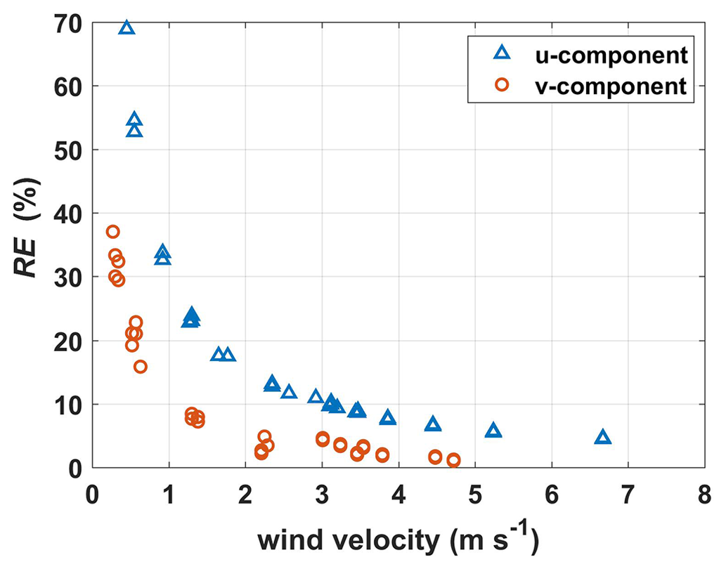
Figure 10 Relationship between the magnitude of the horizontal wind velocity (u,v) and the relative error (RE) from the sensitivity test.

Lastly, it should be noted that the accuracy of the measured georeferenced wind field and turbulent flux from the UAV-based EC system is subject to the combination of many factors, mainly including sensor accuracy, the UAV power plant, the UAV fluctuation (e.g., variation in the UAV attitude and flight height), and the atmospheric conditions during the measurements, etc. This study mainly focused on assessing the effects of sensor precision and the UAV power plant on the measurement errors in the georeferenced wind vector and turbulent flux. Evaluation results gave the lowest limit of the wind field and turbulent flux that the UAV-based EC system can measure reliably. Direct comparison of flux measurements between aircraft and the traditional ground tower is still challenging due to the difference in the measurement height, mechanism (time series for ground EC and space series for aircraft), and instruments (e.g., wind sensor). Previous studies have extensively compared the measurement of fluxes and the wind vector between airborne and ground-based EC methods and found consistent results (Gioli et al., 2004; Metzger et al., 2012; Sun et al., 2021b). At the same time, substantial and consistent over- or underestimations of the measured wind and fluxes by aircraft compared to ground measurements were observed and reported. These differences may be due to several factors, such as vertical flux divergence (the measurement height of the UAV is higher than the ground tower), surface heterogeneity (induced by the larger footprint region of the UAV compared to the ground tower), measurement errors (e.g., window length, resonance noise), and their differences in the platform and sensors. Therefore, in order to evaluate the measurement performance of the UAV-based EC system realistically, it is necessary to conduct a comparison test on the same platform and in the same environment to exclude the influence of these factors.

5 Conclusions and further work

The main objective of this study was to quantitatively evaluate the performance of the developed UAV-based EC system in the measurement of a georeferenced wind field and turbulent flux. In terms of measuring precision, magnitudes larger than 0.7 m s⁻¹ for wind velocity, 0.3 $\mathrm{\mu }\mathrm{mol}{\mathrm{m}}^{-\mathrm{2}}{\mathrm{s}}^{-\mathrm{1}}$ for CO₂ flux, 0.2 W m⁻² for sensible heat flux, and 0.8 W m⁻² for latent heat flux could be reliably measured by the UAV-based EC system. Carefully calibrated offset angles in pitch (ϵ_θ) and heading (ϵ_ψ) were shown to effectively improve the quality of wind field measurements, and the influences of flow distortion and the leverage effect on the wind measurement were minimal and could be ignored. The influence of resonance noise on the measurement of air temperature and water vapor was small (typically <1 % for their variance and flux covariance), but the influence on the measurement of CO₂ (around 5 % for variance and flux covariance) was relatively large.

The relevance of the calibration parameters (ε_r, ϵ_ϕ, ε_ψ, ε_θ) for the measurement of the georeferenced wind vector and turbulent flux was also assessed based on two sensitivity tests. The measurements of the georeferenced wind vector and turbulent flux were insensitive to the errors in ε_r and ϵ_ϕ, while uncertainties in the ε_θ and ε_ψ calibration parameters had the strongest effects on the measurements. Because of ε_θ determining the magnitude of the vertical wind, its error will lead directly to uncertainties in vertical wind measurement and then propagate the uncertainties to the measured turbulent flux. Errors in ε_ψ have a direct effect on the measurement of horizontal wind and to some extent the measurement of turbulent flux. Therefore, these two calibration parameters need to be calibrated carefully. Conducting the UAV-based EC measurement when the wind velocity is larger than 3 m s⁻¹ can lead to more stable and reliable (RE<10 %) results of the wind speed measurement compared to a relatively windless environment.

Finally, we concluded that the developed UAV-based EC system measured the georeferenced wind field and turbulent flux with sufficient precision. The lift-induced upwash and leverage effect had almost no effect on the measurement of the georeferenced wind vector. The resonance effect caused by the operation of the engine and propeller mainly affected the measurement of CO₂, and its effect on variance and flux covariance was around 5 %. The quality of the ε_ψ and ε_θ calibration parameters has a significant effect on the measurements of the georeferenced wind vector and turbulent flux, which underscores the importance of careful calibration. The UAV-based EC system has several advantages over occupied aircraft, including less turbulence disturbance in wind measurement, lower measurement altitude (above ground level), simpler operation, and lower operating costs, etc. Meanwhile, there are still some challenges that need to be overcome like, for example, how to effectively isolate the resonance noise, how to directly evaluate the measurement performance of the UAV-based EC system by comparing it with the traditional tower-based EC instruments, and how to properly interpret the instantaneous flux from aircraft. Future research may include the development of a new UAV-based EC system with the following improvements: (1) a new electro-powered UAV platform with the advantages of being quieter (low noise) and having a low cruising speed; (2) a ground-vehicle-based validation platform to enable direct comparative evaluation of the UAV-based EC system with traditional ground EC methods under near-identical environmental conditions; (3) a graphics-based real-time monitoring system to make it possible to change the flight pattern according to real-time data; and (4) a number of integrated field observation experiments that combine tower-based EC networks, OMSs, and multi-source satellite RS to further prompt the development of theory and methodology for airborne flux measurements. Ultimately, the versatility of the UAV-based EC system as a low-cost and widely applicable environmental research aircraft will further improve our understanding of the energy- and matter-cycling processes at regional scales.