the Creative Commons Attribution 4.0 License.
the Creative Commons Attribution 4.0 License.
 | 27 Aug 2024
ampycloud: an open-source algorithm to determine cloud base heights and sky coverage fractions from ceilometer data
Frédéric P. A. Vogt
Loris Foresti
Daniel Regenass
Sophie Réthoré
Néstor Tarin Burriel
Mervyn Bibby
Przemysław Juda
Simone Balmelli
Tobias Hanselmann
Pieter du Preez
Dirk Furrer
Ceilometers are used routinely at aerodromes worldwide to derive the height and sky coverage fraction of cloud layers. This information, possibly combined with direct observations by human observers, contributes to the production of meteorological aerodrome reports (METARs). Here, we present ampycloud, a new algorithm, and its associated Python package for automatic processing of ceilometer data with the aim of determining the sky coverage fraction and base height of cloud layers above aerodromes. The ampycloud algorithm was developed at the Swiss Federal Office of Meteorology and Climatology (MeteoSwiss) as part of the AMAROC (AutoMETAR/AutoReport rOund the Clock) program to help in the fully automatic production of METARs at Swiss civil aerodromes. ampycloud is designed to work with no direct human supervision. The algorithm consists of three distinct, sequential steps that rely on agglomerative clustering methods and Gaussian mixture models to identify distinct cloud layers from individual cloud base hits reported by ceilometers. The robustness of the ampycloud algorithm stems from the first processing step, which is simple and reliable. It constrains the two subsequent processing steps that are more sensitive but also better suited to handling complex cloud distributions. The software implementation of the ampycloud algorithm takes the form of an eponymous, pip-installable Python package developed on GitHub and made publicly accessible.
- Article
(6926 KB) - Full-text XML
- BibTeX
- EndNote


Ceilometers are being used at numerous aerodromes worldwide to derive autonomously the base height and sky coverage fraction of cloud layers (Wauben et al., 2006; ICAO, 2011; de Haij et al., 2016). These parameters form an essential component of meteorological aerodrome reports (METARs; WMO, 2022). These compact telegrams provide a detailed description of the current meteorological conditions at and around the aerodrome ground to pilots, air traffic controllers, and aerodrome safety services. Regulations from the International Civil Aviation Organization (ICAO) and the corresponding European Commission of Implementing Regulation (CIR, EU373) dictate that METARs should be issued at 30 min intervals – or less in the case of a rapid change in terms of operational significance in the meteorological conditions. Depending on local agreements, the latter situation leads to a SPECI (with the same template as METARs) or a local special report (SPECIAL – with the same template as local routine reports, known as MET REPORTs). METARs and/or SPECIs are representative of the whole aerodrome and are thus mainly used by pilots for flight planning, while MET REPORTs and/or SPECIALs are representative of the threshold and touchdown zone of a specific runway and are mostly used for the management of landing and departure operations by air traffic controllers (ATCs).
The first METAR in Switzerland was issued in 1969 (Willemse and Furger, 2017). The Swiss Federal Office of Meteorology and Climatology (MeteoSwiss) is currently responsible for the production of METARs at the Swiss civil aerodromes. These include the international aerodromes of Geneva (ICAO code: LSGG) and Kloten (ICAO code: LSZH) and eight regional aerodromes. Since 2007, this production has been conducted using the SM/\RT (System for Meteorological Automated ReporTing) software that has been fully developed and maintained by MeteoSwiss. SM/\RT is comprised of both a backend component and a frontend component. The backend is responsible for the data collection from meteorological sensors and includes algorithms for the generation of METAR, MET REPORT, and SPECIAL proposals every minute. The frontend includes the SM/\RT editor, which is used by the aeronautical meteorological observers (AMOs) to compile and send the reports (supported by the message proposals) and a series of “viewers” showing, for example, the real-time data from meteorological sensors on different runways, among others.
The 24/7 automation of METARs is a challenging objective that has been pursued by several meteorological services over the years (see, e.g., Leroy, 2006; Wauben et al., 2006; Hartley and Quayle, 2014; JMA, 2022). With its AMAROC (AutoMETAR/AutoReport rOund the Clock) program, MeteoSwiss is no exception (MeteoSwiss, 2022). At first, the automatic METAR, MET REPORT, and SPECIAL proposals generated by SM/\RT at LSGG and LSZH were systematically reviewed and adjusted by AMOs during the aerodrome's operational hours (05:30–23:30 LT). Since November 2016 at LSGG and since April 2021 at LSZH, during non-operational hours only, SM/\RT-generated METARs have been issued without any human interaction. At LSGG, they have been distributed around the clock since 1 December 2024 and are referred to as AUTO METARs, AUTO MET REPORTs, and AUTO SPECIALs.
Deriving cloud base heights and sky coverage fractions from ceilometer data requires dedicated software. A pioneering algorithm assembled by Esbjörn Olsson at the Swedish Meteorological and Hydrological Institute (SMHI) in 1995 was subsequently shared with ceilometer manufacturers Vaisala and Eliasson (at least), who further developed it (Britt Nordberg, SMHI, private communication, 2022). The original SMHI algorithm was also the base for the software deployed at aerodromes in the Netherlands by the Royal Netherlands Meteorological Institute (KNMI) (Wauben, 2002). In the Unites States, the “sky condition algorithm” developed for the Automated Surface Observing Systems (ASOS; Nadolski, 1998) is another example.
Despite their widespread use, very little detailed information exists on these different algorithms beyond the fact that they rely on clustering methods. None of the associated software are open-source, and several are, in fact, considered to be trade secrets. As a result, the national weather services who want to have full control over their software are often forced to re-develop custom algorithms and/or associated software from scratch. The opacity surrounding the different algorithms responsible for generating AUTO METARs worldwide prevents any external (neutral) assessment, validation, and/or intercomparison of their capabilities. Furthermore, the lack of open-source software and publicly available documentation hinders the improvement of algorithms through collaborative work. This opacity may also impede the combined use of distinct ceilometer types at a given site.
In this article, we present ampycloud, a new open-source algorithm, and its associated Python package designed to derive the base height and sky coverage fraction of cloud layers from ceilometer data. ampycloud is part of the SM/\RT backend. It is one among several new and/or improved algorithms developed at MeteoSwiss as part of the AMAROC program, with the goal of generating fully automated METAR reports at Swiss civil aerodromes. The algorithm itself is introduced in Sect. 2. The ampycloud Python package, its computational performance and accuracy, and its deployment and operational use by MeteoSwiss are all described in Sect. 3. The known limitations of ampycloud are discussed in Sect. 4, together with different enhancement possibilities. Our conclusions are presented in Sect. 5.
Throughout this article, heights are reported in units of feet (ft), with 1 ft = 0.3048 m.
2.1 Requirements
An algorithm that has to operate 24/7 without direct human supervision should meet specific requirements. In particular, it should be
- 1.
robust (any input, no matter its plausibility, is processable) and
- 2.
reliable (any input results in a reasonable output).
For the specific case of generating information to be used in METARs, the algorithm should also be designed to be
- 3.
stable (a small change in the input results in a small change in the output),
- 4.
conservative (if two possible outputs are equally probable, the worst one – from an aerodrome and/or flight safety perspective – is to be favored), and
- 5.
fast (the processing time should be less than ∼1 min in order to issue SPECIs or SPECIALs as soon as they are warranted).
Furthermore, any meteorological algorithm can also benefit from being
- 6.
physics-based (methods and parameters have a physical interpretation and justification).
This can ease, for example, the selection of parameter values and the identification of specific shortcomings in the algorithm and, thus, of elements with potential for improvement. A supervised machine learning method trained to reproduce (subjective) cloud observations would be an example of a non-physics-based algorithm, which is generally more difficult to interpret and often expensive to maintain (typically denoted as a black box; see, e.g., Sculley et al., 2015; Rudin, 2019). ampycloud was developed with these different requirements in mind.
One should note that the ampycloud algorithm was not developed because the other algorithms serving similar goals and being used at aerodromes worldwide are unfit for their purpose. Rather, it is the lack of information and transparency about their design that led MeteoSwiss to assemble ampycloud, in addition to ensuring its long-term maintainability and extendability.
2.2 Algorithm concept
The ampycloud algorithm is composed of three sequential steps, which we refer to as slicing, grouping, and layering. The slicing step is designed for robust detection of the main cloud layers. It is meant to constrain the ampycloud outputs to a reasonable range, no matter the input data. The high degree of reliability in this step is achieved by reducing its capacity to handle complex cloud distributions. Specifically, the slicing step is subject (by design) to two pitfalls:
-
It can split cloud layers that span a broad range of heights and/or have a marked upward or downward trend.
-
It can aggregate close-but-distinct cloud layers.
The grouping and layering steps of the ampycloud algorithm are designed specifically to refine the slicing step. The slicing, grouping, and layering steps of ampycloud thus form a coherent sequence, with each step operating on the outcome of the previous one.
ampycloud reports compliant METAR codes1 for up to three cloud layers at most, with the following selection rules (ICAO, 2018):
-
The lowest layer is always reported.
-
The second layer up is reported if it has a sky coverage of SCT or more.
-
The third layer up is reported if it has a sky coverage of BKN or more.
It must be stressed that, when used on its own, ampycloud can comply with only a subset of the ICAO's rules for cloud reporting in the sense that it is designed to characterize cloud layers with well-defined bases only. The ampycloud algorithm does not concern itself with the question of whether a vertical-visibility (VV) code should be reported instead of a cloud base height in METARs. At MeteoSwiss, this aspect is being handled by different tools within the SM/\RT infrastructure. Obscuration of the sky by fog or snow is also being handled by a separate algorithm within SM/\RT. ampycloud does not consider the question of convective cloud detection (CB/TCU) either, which is best done using a combination of lightning and weather radar data. Regulations state that “if there are no clouds of operational significance and no restriction on vertical visibility and the abbreviation CAVOK is not appropriate, the abbreviation NSC should be used” (ICAO, 2018). Given its scope, ampycloud cannot decide whether a CAVOK code is appropriate and will therefore always return the code NSC if there are no cloud layers found below the minimum sector altitude (MSA). If no clouds are detected at all by the ceilometers, ampycloud will return the code NCD. Importantly, users should bear in mind that because ampycloud does not and cannot handle CB and TCU cases, any NCD or NSC code issued by ampycloud may need to be overwritten by the user in certain situations.
2.3 Input data
The World Meteorological Organization (WMO) defines a cloud base as “a zone in which the obscuration corresponding to a change from clear air or haze to water droplets or ice crystals causes significant changes in the profiles of the backscatter and extinction coefficients” (WMO, 2021). Ceilometers deployed at aerodromes worldwide are designed to detect such changes in backscatter coefficient profiles (ICAO, 2011), which are typically reported in the form of cloud base and/or vertical-visibility (VV) hits (see, e.g., Vaisala Oyj, 2015; Campbell Scientific, 2021; OTT HydroMet, 2022) but with significant differences between ceilometer types or models (Martucci et al., 2010; Görsdorf et al., 2016, 2018). ampycloud is designed to use cloud and VV hits acquired by one or more ceilometers over a time interval Δt to characterize the cloud base heights and sky coverage fractions above a specific area. This is a well-established approach (Wauben et al., 2006; Nadolski, 1998; Wauben et al., 2006; ICAO, 2011; WMO, 2021). It relies on the wind dragging the cloud distribution over the ceilometer line(s) of sight to enhance their otherwise very restricted spatial sampling capabilities and, thus, to obtain a more representative view of the sky. The longer the time interval or the larger the wind speed, the better the spatial representativity of the dataset but the worse the view of the “current” state of the sky (especially in the case of rapidly changing conditions).
Table 1Summary of the ceilometers deployed at the LSGG and LSZH civil aerodromes as of May 2024. The MSA values are expressed in units of feet above aerodrome level (ft a.a.l.; MeteoSwiss, 2023).
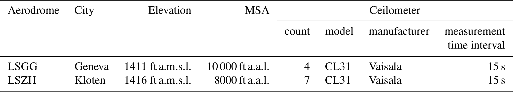
ampycloud requires every cloud and VV hit h to be comprised of four elements:
with hhgt being the cloud base height above aerodrome level (a.a.l.; in ft); htme being the observation time (in seconds – either as absolute Unix time or relative to a specific event, e.g., the most recent ceilometer data in the set); hcid being a ceilometer reference ID; and htpe being the hit type, which will be explained below. The models and numbers of ceilometers in operation at LSGG and LSZH are summarized in Table 1. The use of ampycloud is not restricted to any specific model of ceilometer in particular, provided that individual hits can be specified following Eq. (1). One should note that, for the moment, ampycloud cannot use full backscatter profiles to derive cloud base hits independently from the ceilometers' proprietary software. Implementing such a capability could enhance the robustness and traceability of the hit derivation, but it would not fundamentally change the behavior of the ampycloud algorithm in itself.
ampycloud can process measurements from any number of ceilometers and makes no distinction between them. Data from different ceilometers are analyzed together, independently of the spatial distribution of the instruments on the ground. The specification of hcid for every hit ensures that a correct estimation of the sky coverage fraction can be made under the assumption that cloud layers have a unique base per time step per ceilometer line of sight. Without a value of hcid to differentiate sightlines, two simultaneous measurements from distinct ceilometers would not be distinguishable and, thus, would possibly become contradictory. One can, of course, apply ampycloud to a smaller number of ceilometers, e.g., to a specific subset associated with a given runway to generate local routine reports (AUTO MET REPORTs).
Aside from operational redundancy, one benefit of using multiple ceilometers to characterize cloud layers lies in the boost of the probability of detecting clouds (clear sky) for cloud layers with very low (very high) sky coverage fractions. This fact, demonstrated experimentally by Wauben (2002), is illustrated in Fig. 1. The ability to better distinguish between OVC and BKN layers may not be a crucial benefit in itself, given that both categories imply the existence of an (operationally relevant) “ceiling”. However, using multiple ceilometers can also contribute to a reduction in the cases of gross overestimation or underestimation of sky coverage fractions under slow-moving conditions (i.e., low wind with quasi-stationary clouds), provided that the horizontal separation between ceilometers is larger than the applicable cloud characteristic scale length (Slobodda et al., 2015; Denby et al., 2022).
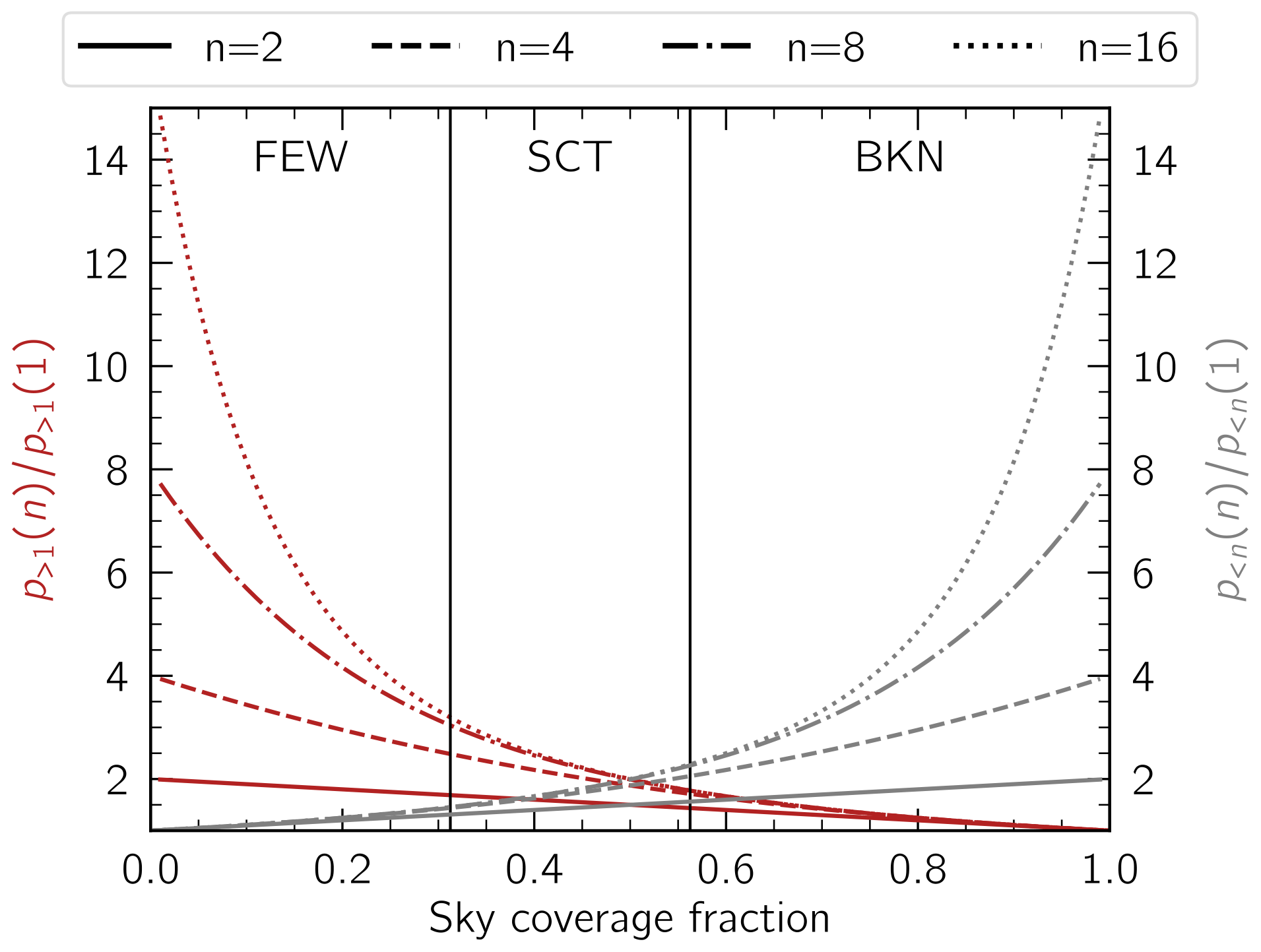
Figure 1Theoretical improvement in the probability of getting at least one cloud hit with n ceilometers p>1(n) compared to only one ceilometer p>1(1) (at any one specific moment in time), ignoring any spatial scale considerations in the cloud and ceilometer distributions (red curves). The mirrored probabilities of detecting at least one clear sightline p<n are shown in gray.
It is important to consider the hit type htpe to derive a correct estimation of the sky coverage fraction of cloud layers. Typically, ceilometers can report multiple cloud base heights and/or vertical visibilities with every observation (i.e., at every time step). For example, the ceilometers deployed at LSZH and LSGG report, for every measurement, either up to three distinct cloud base heights or a vertical visibility and signal range (Vaisala Oyj, 2015). The latter occurs if the sky is obscured (for example, due to fog or precipitation). The hit type htpe is used to keep track of these differences. It must be stressed, however, that ampycloud does not treat vertical-visibility (VV) hits differently to regular hits. Every hit h inputted into ampycloud is treated as a regular cloud base hit. It is up to the user to decide if and when VV hits should be provided to ampycloud and whether they need to be pre-processed in any way before doing so. Not passing VV hits to ampycloud can lead to an underestimation of the sky coverage fraction. However, VV hits can also be caused by precipitation that might lead to the reporting of spurious (lower) cloud layers. As of the release of ampycloud v1.0.0, MeteoSwiss inputs any VV hits reported by CL31 ceilometers into the code without further selection or modification of their reported height.
ampycloud works in a relative time space and will automatically assign to each measurement a time difference with respect to the latest one. The algorithm poses no restriction on the time interval Δt over which cloud and VV hits can be bundled. For historical reasons, cloud and VV hits spanning Δt=15 min for AUTO METARs (from all ceilometers) and Δt=6 min for AUTO MET REPORTS (from specific pairs of ceilometers associated with a given runway) serve as inputs for ampycloud at LSGG and LSZH. Users can, however, freely choose to collect cloud and VV hits over a longer time interval: ampycloud will process whatever collection of cloud and VV hits it receives as input.
2.4 The parameters of ampycloud
The parameters of ampycloud are summarized in Table 2. Those specifically related to the slicing, grouping, and layering steps will be discussed in Sect. 2.6. The other ampycloud parameters are responsible for the generation of compliant METAR codes. It must be stressed that the default values provided in Table 2 for the different parameters are not necessarily applicable universally. Depending on their needs and/or instrumental setups, some users may wish to consider adjusting some of them, for example Θ0 and/or Θ8. Θ0 is the maximum (absolute) number of cloud hits required for a given slice, group, or layer to still be considered to be NCD by ampycloud; Θ8, on the other hand, is the maximum number of “holes” (i.e., non-detection of clouds) required for a given slice, group, or layer to be considered to be OVC by ampycloud. We adopt Θ0=3 hits (Θ8=1 hole) at LSGG to avoid assigning cloud layers with low (high) sky coverage fractions to noise fluctuations and false cloud detections (e.g., returns by airplanes passing above a ceilometer2).
Table 2Parameters (and associated default values) controlling the behavior of ampycloud as of version 2.0.0 of the eponymous Python package. The values of each parameter were chosen and verified using specific examples and a large-scale statistical assessment of the algorithm's accuracy (see Sect. 3.4). The meaning and role of each parameter are described in detail in the associated article sections. Note that the parameter specifying the aerodrome's MSA must be specified in ft a.a.l. (and not in ft a.m.s.l.).
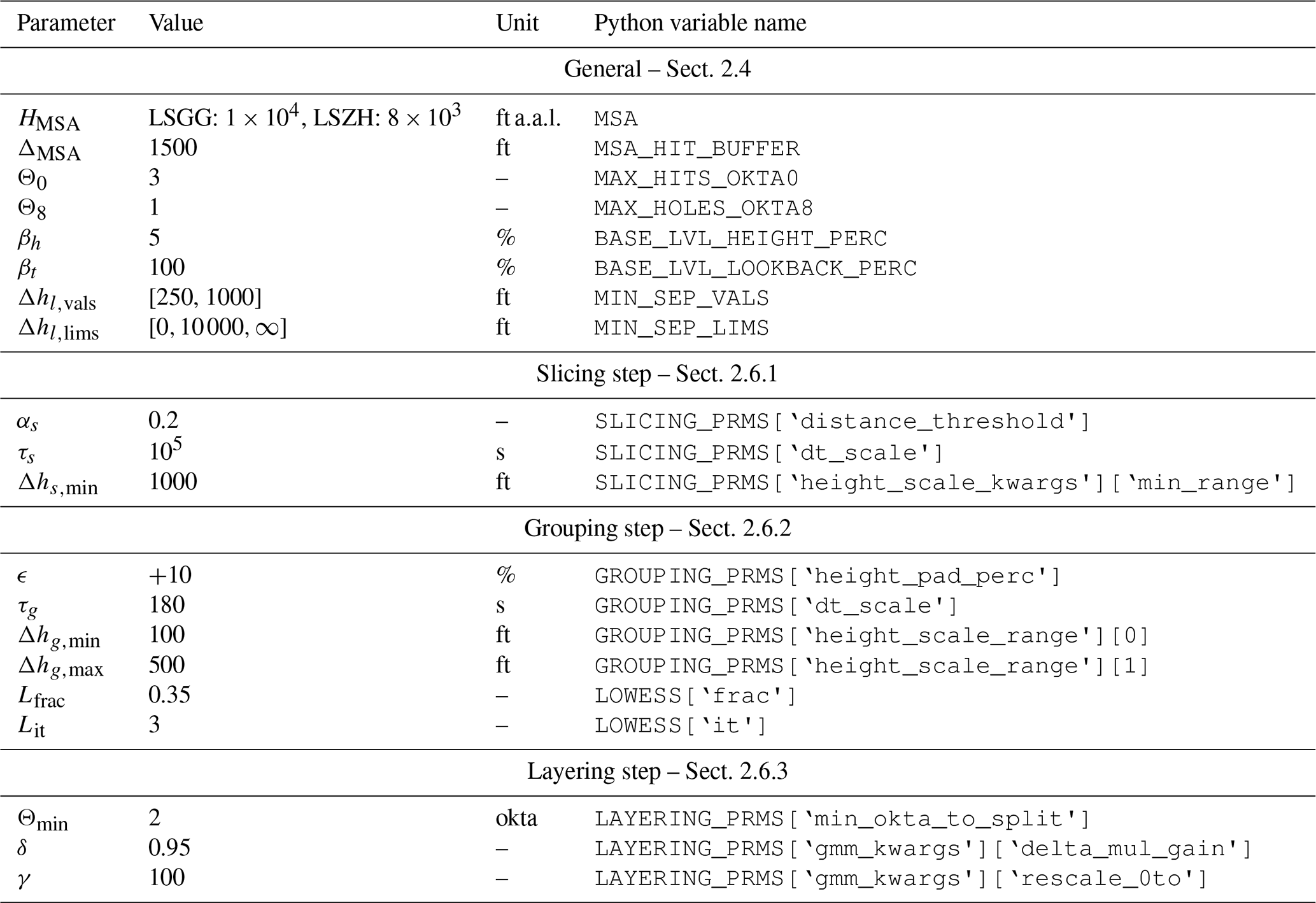
ampycloud computes the base height of a given slice 𝒮i, group 𝒢i, or layer ℒi as the βh percentile of the sorted hit heights within the βt percentage of the most recent hits in the slice, group, or layer. We adopt βh=5 % and βt=100 % by default, such that all hits within a given slice, group, or layer are used to derive the height of its base. It must be stressed that ampycloud does not apply any weighting to the different hits prior to computing the base height or sky coverage fraction of a specific slice, group, or layer. This choice is motivated by the following argument. ampycloud bundles ceilometer data over a certain time interval Δt to obtain a (more) representative view of the sky. All cloud hits, irrespective of their age, are equally trusted in order to identify cloud layers. It thus makes sense to also treat them all equally when computing the cloud base height of the identified layers. For ampycloud, old hits are not less valid: they merely represent the state of the sky further away than the ceilometer lines of sight. Nonetheless, if a user were to prefer the cloud base heights to be more representative of the most recent hits within a slice, group, or layer, the βt parameter can be set to lower values, e.g., βt=30 %. Note that changing the value of βt does not have any effect on the sky coverage fraction measurements.
As will be discussed in Sect. 2.6.3, the layering step is able to separate cloud layers that are very close to one another if they are well defined. The grouping step can also lead to sub-groups in very close proximity to each others when they are well defined, which can be problematic from a user perspective. The parameters and are introduced to ensure that groups and layers identified in the second and third steps of the algorithm are sufficiently far apart. Essentially, the base height of cloud groups or layers must be at least Δhl,vals[k] ft apart if they have a base height in the range , with .
In the ampycloud Python package, two additional parameters – HMSA and ΔMSA – are used to crop any hit with a height above aerodrome level that is significantly beyond the applicable minimum sector altitude (MSA), namely beyond HMSA+ΔMSA, where HMSA is the MSA value (specified in ft a.a.l., e.g., 10 000 and 8000 ft a.a.l. for LSGG and LSZH, respectively), and ΔMSA is a buffer to properly treat cloud layers whose thicknesses and/or fluctuations extend slightly beyond the MSA.
2.5 The ampycloud diagnostic diagram
The ampycloud diagnostic diagram for a mock dataset, designed to demonstrate the role of each sequential step of the algorithm, is presented in Fig. 2. The details of each step will be discussed in Sects. 2.6.1 to 2.6.3. We do already note, however, that, with the first robust slicing step being fine-tuned by the subsequent grouping and layering of cloud structures, the ampycloud algorithm is not overly sensitive to any of its parameters in particular.
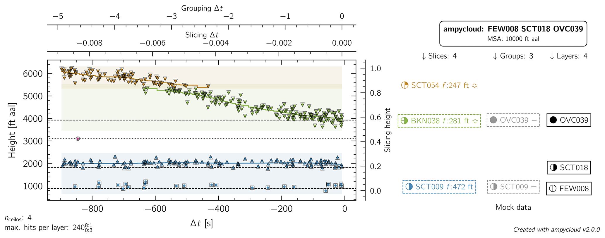
Figure 2ampycloud diagnostic diagram for a mock (demonstration) dataset with a 900 s look-back time, designed to illustrate the slicing, grouping, and layering steps of the algorithm. See Sect. 2.5 for a detailed description of the different elements of this figure.
Individual (artificial) cloud hits are visible in Fig. 2 as colored points in the diagram. This dataset simulates observations from four ceilometers, each performing (asynchronous) observations every 15 s, with a look-back time of 900 s. The color of each hit corresponds to the horizontal slice 𝒮i (with in this example) they are assigned to by the first step of the algorithm. The colored rectangles expand above (below) the maximum (minimum) height of each slice 𝒮i, with being a parameter of ampycloud and T(𝒮i) being the thickness of the slice 𝒮i. This vertical range is used to identify overlapping slices that may require grouping. Colored lines correspond to LOWESS (locally weighted scatterplot smoothing) fits of the cloud hit distribution within each slice: they are used to compute the slice fluffiness f (in ft) used in the grouping step, which will be formally defined in Eq. (4). The black squares, triangles, and circles around each cloud hit denote the final layer ℒi (with in this example) they are assigned to as a result of the third step of the algorithm. The intermediate groups 𝒢i (with in this example) identified by the second algorithm step are not shown for readability purposes.
Secondary x and y axes on the right and at the top of the diagram show the rescaled hit time and height axes used for the slicing and grouping steps. The characteristics of each slice 𝒮i, group 𝒢i, and/or layer ℒi with a sky coverage fraction of FEW or more are shown on the right-hand side of the diagram, including the measured sky coverage in oktas. Overlapping slices are tagged with ≎. Groups for which the layering step was executed are tagged with −, =, or ≡ depending on whether one, two, or three distinct sub-layers were identified. Cloud slices, groups, or layers found are reported according to METAR syntax, i.e., [FEW|SCT|BKN|OVC]nnn, where nnn is the cloud slice, group, or layer height in hundreds of feet above aerodrome level. Not all cloud slices, groups, or layers need to be reported according to the ICAO rules (ICAO, 2018). The relevant ones are boxed.
The final selection of cloud layers is shown in the top right of the figure. To the bottom left of the diagram, the number of ceilometers contributing data to the diagram is indicated explicitly, alongside the maximum number of cloud hits possible per cloud layer (240 in this example) corresponding to the total of the individual time steps reported by each ceilometer. The superscripts and subscripts indicate the values of the parameters Θ8 and Θ0 (with the format 8:Θ8 and 0:Θ0). One should note that the number of slices, groups, and layers reported on the right-hand side of the diagrams do include clusters that are comprised of less than Θ0 hits, as illustrated by the single cloud hit at −800 s (3100 ft a.a.l.) that gets assigned its own slice, group, or layer as indicated by the dotted horizontal line in the diagram.
2.6 The three ampycloud steps
2.6.1 Slicing
Given a set of hits gathered over a time interval Δt, the first ampycloud step consists of the identification of (horizontal) height slices 𝒮i. The algorithm does this using an agglomerative clustering approach with an average linkage criterion and a Manhattan metric3. The key to the robustness of this processing step lies in the rescaling of the cloud base hits along both the time and height dimensions, applied prior to the clustering.
Given the minimum and maximum hit heights hmin and hmax, the interval [hmin;hmax] is mapped linearly onto the interval [0;1]. If, however, , it is the following interval:
with length Δhs,min being mapped onto [0;1] instead. Essentially, Δhs,min (which is a parameter of ampycloud; see Table 2 for the complete list) ensures that cases with a small height dispersion do not get over-stretched and, thus, “over-sliced”.
Along the time axis, hits are rescaled (i.e., normalized) by a very large number τs. If τs is large enough, the distance between hits along the time direction becomes essentially negligible in the rescaled space. As a result, the measure of the linkage distance – used by the agglomerative clustering method to decide whether to merge hits or not – is dominated by the height component of the hits4. In this rescaled space, a distance threshold αs will identify horizontal slices of hits whose rescaled mean heights are separated by no more than αs. With τs≫1, the value of αs represents the maximum thickness of individual horizontal slices, expressed as a fraction of the total height range in the sample. Hence, at most, distinct slices can be identified by ampycloud, and these will never be thinner than . For the default ampycloud parameters, slices, and ft.
This rescaling scheme is well suited to identifying vertically stratified cloud layers with a stable base as a function of time. However, it is ill-suited for cloud layers with a thick and/or time-varying base height, where the variation is larger than . This shortcoming is illustrated in Fig. 2, with the top layer being sliced in two. The slicing step is also ill-suited to distinguishing isolated cloud layers separated by less than . This is illustrated with the bottom two cloud layers in Fig. 2, which are detected as a single slice.
The grouping and layering steps of ampycloud are designed specifically to handle these limitations of the slicing step. As a result, the output of ampycloud is not very sensitive to the values of Δhs,min and αs in that any over-slicing or under-slicing of hits is compensated for by the subsequent processing steps.
2.6.2 Grouping
This processing step is designed to handle the over-slicing of coherent cloud hit structures as a result of a broad height span or marked upward or downward trends of a cloud layer (as illustrated by the top two slices in Fig. 2). It begins by identifying so-called overlapping slices. These are flagged by the symbol ≎ in the ampycloud diagnostic diagrams. By (our) definition, slices i and j overlap if one of the following two conditions is met:
with min(𝒮i) and max(𝒮i) being the minimum and maximum hit heights of the slice 𝒮i, being the thickness of the slice 𝒮i, and ϵ being a parameter of the ampycloud algorithm. Setting ϵ=0 would result in a strict overlap diagnostic. To avoid edge cases with identical minima and maxima in terms of cloud hit heights, as well as to account for natural cloud base height fluctuations, we adopt a default value of ϵ=10 % to slightly pad the slices by a fraction of their thickness before checking for overlap. For example, the top two slices in Fig. 2 (green and red) overlap according to this criterion with our adopted value of %.
Having identified a set of n overlapping slices, ampycloud uses an agglomerative clustering method with a single linkage criterion and an Euclidean metric to identify coherent sub-groups gk, with . Each sub-group gk is subsequently assigned to a master group 𝒢i based on the slice 𝒮i to which the majority of the hits in group gk belong. Hence, the ampycloud grouping of n overlapping slices will result in no fewer than one and no more than n master groups 𝒢. In other words, there can be no more groups 𝒢 than slices 𝒮. Essentially, the slicing step of ampycloud constrains the grouping step, which would otherwise be overly sensitive to noisy datasets. It also ensures that sparse cloud layers do not get broken into sub-groups along the time axis.
The hit heights and (relative) times are rescaled prior to being inputted into the (single-linkage) agglomerative clustering method of the grouping step. The rescaling is performed separately for each set of overlapping slices. In all cases, the time-axis-scaling factor is set to τg. The height-scaling factor is taken to be the minimum slice fluffiness fmin in the overlapping bundle, provided that , Δhg,max]. If fmin is larger (smaller) than Δhg,max (Δhg,min), the latter value is used as the height-rescaling factor instead. The fluffiness f of a slice 𝒮i is a measure of the spread of cloud hits around the smoothed cloud height trend, which we formally define as follows:
with N being the number of cloud hits in the slice, hhgt,k being the individual cloud hit heights, and L(htme,k) being the LOWESS-derived (Cleveland, 1979) height corresponding to the hit time htme,k. The LOWESS algorithm5 is used to robustly measure the mean cloud hit height as a function of time using a series of localized weighted linear regressions. The LOWESS fit of each slice in Fig. 2 is shown using colored lines. It relies on two parameters: the fraction of slice hits (along the time axis) Lfrac to be used for each linear regression and the number of iterations Lit for each fit. The LOWESS fit of a given slice 𝒮i is fully sensitive to coherent cloud hit height fluctuations affecting more than a fraction Lfrac of the slice's cloud hits. The smaller the fractional duration of a specific height variation is below Lfrac, the smaller its influence on the resulting LOWESS fit is. By default, we adopt Lfrac=0.35, which corresponds to a sensitivity timescale of ∼5 min for a uniform cloud hit distribution observed over an interval of 15 min. The default value of Lit=3 ensures that the final LOWESS fit is not affected by spurious hits with significant height offsets. We note that, although the ampycloud algorithm uses the fluffiness of (overlapping) slices 𝒮 only for the grouping step, the ampycloud Python package computes the fluffiness of every slice 𝒮i, group 𝒢i, and layer ℒi by default.
The agglomerative clustering method with a single-linkage criterion uses the closest elements of sub-clusters to decide whether to merge them or not. With a linkage distance of 1 fixed inside ampycloud, τg and the slice fluffiness determine the maximum distance (in time and height, respectively) below which two cloud hits will be assumed to belong to the same cloud structure. Unlike the slicing step that ignores the time information (with τs⋙1), the grouping step is much better suited to tracking coherent height variations as a function of time, as demonstrated in Fig. 2. In that example, the hits in the top two slices (red and green at 3800 and 5400 ft, respectively) are grouped into a single master group with a base at 3800 ft.
2.6.3 Layering
By design and as illustrated in Fig. 2, the slicing step will inevitably bundle distinct cloud structures into common slices if isolated cloud layers are separated by less than . The layering step is designed to correct this shortcoming. It relies on the computation of Gaussian mixture models with one, two, and three components for every master group 𝒢i with a sky coverage fraction of at least Θmin oktas. For each model, the value of the associated Bayesian information criterion BICi is recorded.
Statistically speaking, the best-fitting model out of the three will have the lowest BIC score. However, cloud hits belonging to a given cloud layer typically will not follow a Gaussian distribution. Using the relative likelihood (and associated probabilities) of different Gaussian mixture models to identify the most likely number of components in a group would thus typically lead to an overestimation: not because more components represent a better fit but rather because they represent a somewhat-less-bad-but-still-terrible one (see Appendix A for details). Hence, ampycloud does not simply follow this criterion alone to decide whether a given group requires being broken up. The following selection approach is adopted instead.
The starting assumption for each group 𝒢i is that it does not contain sub-layers. Moving sequentially through the Gaussian mixture models with one, two, and three components, ampycloud will identify n sub-layers if . Essentially, ampycloud assumes n sub-layers to be present only if the decrease in the model's BIC score over the current best number of sub-layers is greater than (1−δ).
BIC scores are sensitive to the data values in the underlying dataset. To alleviate the consequences of this fact, ampycloud rescales the height range of every individual master group 𝒢i between 0 and γ prior to searching for sub-layers. A given δ value will thus split groups based upon the relative separation of their sub-layers in terms of their height dispersion, irrespective of whether the groups are located at 2000 or 20 000 ft.
This approach still remains unstable for small datasets. This is why ampycloud will not attempt to break-up groups with a sky coverage fraction of less than Θmin=2 oktas. The adopted values of δ=0.95 and γ=100 imply that two perfectly Gaussian sub-layers would be separated by ampycloud if their means are offset by at least ∼5 standard deviations from one another (see Appendix A for details).
3.1 Implementation
The ampycloud Python package (Vogt et al., 2024) was developed on GitHub (ampycloud, 2024a) as a regular, non-MeteoSwiss-specific, pip-installable Python package. The source code is made available to the general community as open-source software under the terms of the 3-Clause BSD License. As a project, ampycloud follows an approach of continuous integration and continuous delivery. It relies on GitHub Actions to run automated quality, stability, and validity checks; to publish the documentation; and to upload new versions to the Python Package Index (PyPI). The algorithm described in this article corresponds to version 2.0.0 of the ampycloud Python package. The scientific behavior of this version is essentially identical to version 1.0.0, which was deployed at LSGG in November 2023. Version 2.0.0 simply provides a more coherent variable-naming scheme and an improved handling of NSC and NCD codes in addition to a few minor code updates.
As a key dependency of the operational AUTO METAR software of MeteoSwiss, ampycloud must remain robust and stable. An evolution of the code over time is inevitable and even desirable, but it will be carefully controlled. Any future release of the code (and associated changes) will be fully documented in the online documentation of the ampycloud package (ampycloud, 2024b), to which we refer the interested readers for more details on the evolution of the algorithm after the publication of this article. We shall not discuss in extensive detail here the technical implementation of the ampycloud Python package itself. It suffices to say that (1) ampycloud requires cloud and VV hits stored in a suitably formatted Pandas DataFrame as input; (2) the slicing and grouping steps rely on the sklearn.cluster.AgglomerativeClustering() class from the scikit-learn Python package; (3) the layering step relies on the sklearn.mixture.GaussianMixture() class from the same package; and (4) the fluffiness of slices, groups, and layers is computed using the LOWESS algorithm implemented in the statsmodels package. We refer the interested readers to the official ampycloud online documentation (ampycloud, 2024b) for further information on its different classes and functions.
3.2 Deployment at MeteoSwiss
The ampycloud algorithm and associated Python package have been used at LSGG since 31 October 2022 outside the operational hours of the aerodrome, with its outcome being supervised by an AMO during operational hours and used for METAR proposals. The initial version 0.5.0 was replaced by version 1.0.0 of the code on 28 November 2023. Version 2.0.0 of the code, developed as part of the publication of this article, will be deployed in the near future. As of 1 May 2024, ampycloud has been operating (alongside SM/\RT) in standalone mode (i.e., without human interaction) at LSGG during the aerodrome's operational hours.
In the MeteoSwiss operational setup, the ampycloud Python package is imported as an external dependency within a Python service known as the cloud calculator (closed-source software). The cloud calculator is one of several calculators that comprise the autometpy software suite, developed as part of the AMAROC program. The cloud calculator runs on the MeteoSwiss OpenShift container platform, where it stands ready to receive calculation requests. The requests are issued and orchestrated by SM/\RT, which decides how often and with what data the cloud calculator is called. At LSGG, SM/\RT makes three requests to the cloud calculator every minute as follows:
-
in AUTO METAR mode using data from all four ceilometers over the last 15 min
-
in AUTO MET REPORT mode using data from the two ceilometers representative of RWY22 over the last 6 min.
-
in AUTO MET REPORT mode using data from the two ceilometers representative of RWY04 over the last 6 min.
Monitoring the status and computational performances of the cloud calculator is done using a flexible dashboard providing access to various metrics (CPU load, memory use, request time, number of requests, errors). Dedicated log files are also collected and can be queried whenever necessary. Diagnostic plots are produced by a separate calculation request using the same input data for monitoring and debugging purposes, particularly to quickly answer questions from stakeholders.
3.3 Computational speed (performance)
We use the mock dataset presented in Fig. 2 to keep track of the speed performance of the ampycloud package over the course of its development by means of the dedicated GitHub Action (ampycloud, 2024d). With ampycloud v2.0.0, the processing of this dataset takes 0.20 s on average on a 16 in. MacBook Pro 2019 with a 2.3 GHz 8-Core Intel Core i9. On a server running Ubuntu with Linux kernel 6.2 with four cores, the processing lasts 0.30 s (ampycloud, 2024e). These values are representative of ampycloud processing times in general. Among the real examples presented in Appendix B, the case in Fig. B2 takes the most time to process (0.35 s), whereas the case in Fig. B12 takes the least time (0.12 s). These processing times do not include the creation of the ampycloud diagnostic diagrams, which are optional and require an additional ∼2 s per diagram.
3.4 Comparison with reference METARs (accuracy)
We present in Appendix B a series of representative, real examples from the Swiss civil aerodromes. These are meant to illustrate the behavior of the ampycloud algorithm under varying weather conditions. For each case, the actual METAR cloud codes (produced by an AMO at the time) are provided for comparison purposes. To maximize the readability of this article, each case is discussed directly within the figure caption.
Comparing AUTO METAR cloud codes (derived purely from ceilometer observations) with METAR ones (derived fully or in part from AMOs) is evidently subject to a series of fundamental caveats. Both methods have specific strengths and limitations (see, e.g., paragraph 7.4.3.1 in ICAO, 2011). For example, cloud layers in the 1–2 okta range are systematically more difficult to observe at night for human observers, which is not the case for ceilometers (Boers et al., 2010). On the other hand, the exact ceilometer performances can vary depending on air temperature and direct sun exposure. Standard ceilometers typically only sample a small part of the sky immediately above them, whereas AMOs can more easily observe the entire sky (even though the slanted view from a fixed position still limits their ability to detect holes in cloud layers with high sky coverage fractions). Ceilometers will typically require the collection of data over a longer time frame than AMOs to derive the appropriate cloud codes such that METAR cloud codes will typically be more representative of the “instantaneous” situation at the message distribution time when compared to AUTO METARs. Finally, AMOs at Swiss aerodromes (at least) will typically estimate sky coverage fractions independently but remain encouraged to use ceilometer data for their estimation of cloud base heights. The extent to which they do so depends on the weather conditions and the personal inclination of each observer.
Bearing these differences in mind, the overall accuracy of the ampycloud algorithm was evaluated in a statistical sense using a reference dataset of 2128 cases extracted over a 5-year period (2018–2022) from LSGG METARs. Doing such a comparison for LSGG remains meaningful and important: not because METARs represent the absolute truth but rather because AMOs were the existing operational system. Any significant and/or systematic change in the behavior of AUTO METARs with respect to METARs must be characterized, documented, and explained to the relevant civil aviation authority and stakeholders (e.g., air traffic controllers). The 2128 reference cases were selected to provide a representative sub-sample of all the METARs over this period. The case selection focused on operationally relevant situations (according to the METAR, ampycloud, or both). Of the 2128 cases, 71.5 % correspond to a cloud ceiling situation, i.e., the presence of a BKN or OVC cloud layer. Without any pre-selection, the ratio of ceiling cases at LSGG is ∼36 %.
Using the sample of 2128 cases, we present in Fig. 3a comparison of the cloud layers with the highest sky coverage fraction as identified by the ampycloud algorithm and the actual METAR. In 57.8 % of the cases, the ampycloud output is consistent with the METAR and is, at most, one category off in 95.7 % of the cases. The cases where ampycloud differs more significantly (by at least two classes) from the METAR land in two categories. The cases when ampycloud underestimates the sky coverage fraction of the cloud layer (i.e., “misses” – 3.2 % of the cases) are related to situations where cloud layers are not seen by the ceilometers – either because they are not above the line of sight or because the ceilometer signal is blocked by a lower layer. This also explains the 6.3 % of misses where ampycloud returns NCD or NSC and the AMO reports FEW: a situation typically related to stationary cumulus clouds above the Jura mountain range at a distance of ∼12 km from the aerodrome. The “false alarms” (1.2 % of all cases), where ampycloud overestimates the sky coverage fraction of the cloud layer by at least two classes, are nearly all related to cases of low-level fog being seen as a low-level cloud layer by the ceilometers. For operations, these cases are treated by a separate vertical-visibility algorithm, which also uses horizontal visibility and present weather information (i.e., the presence of snow and fog).
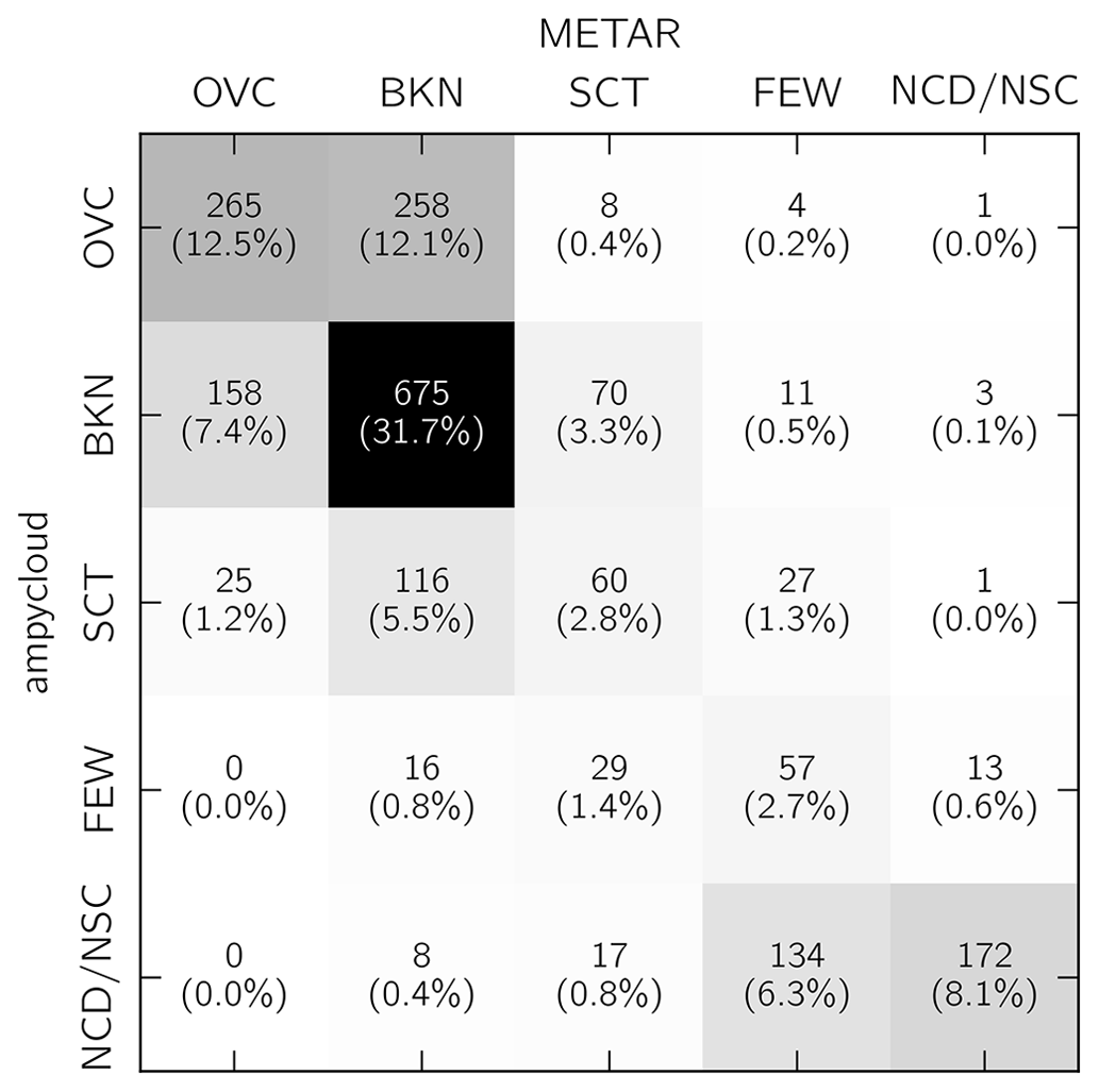
Figure 3Matrix comparing the categorization of the cloud layers with the highest sky coverage fraction identified by the ampycloud algorithm (vertical axis) with the actual METAR validated by an AMO (horizontal axis) for a reference dataset of 2128 cases assembled from LSGG observations. Boxes located above the diagonal can be associated with false alarms where ampycloud finds a sky coverage fraction that is larger than the METAR. The cases below the diagonal can be understood as misses, where the opposite happens.
The same information can also be presented using operationally relevant categories. In Fig. 4, we present the ability of ampycloud to report a cloud ceiling. The ampycloud identification of a ceiling (or absence thereof) is in agreement with the corresponding METAR 87.7 % of the time. The comparison of Figs. 3 and 4 shows that ceiling false alarms (4.6 %) and misses (7.8 %) are dominated (respectively) by cases where ampycloud characterizes an SCT layer as BKN (3.3 % of the cases) and a BKN layer as SCT (5.5 % of the cases). These two types of situations are a direct consequence of the limited spatial-sampling capabilities of ceilometers. Of course, one cannot rule out the possibility that some of these mismatches are driven by the limited ability of human observers to distinguish between cloud layers with a sky coverage fraction of slightly more or less than 56.25 % (which corresponds to the limit between SCT and BKN; see Boers et al., 2010).
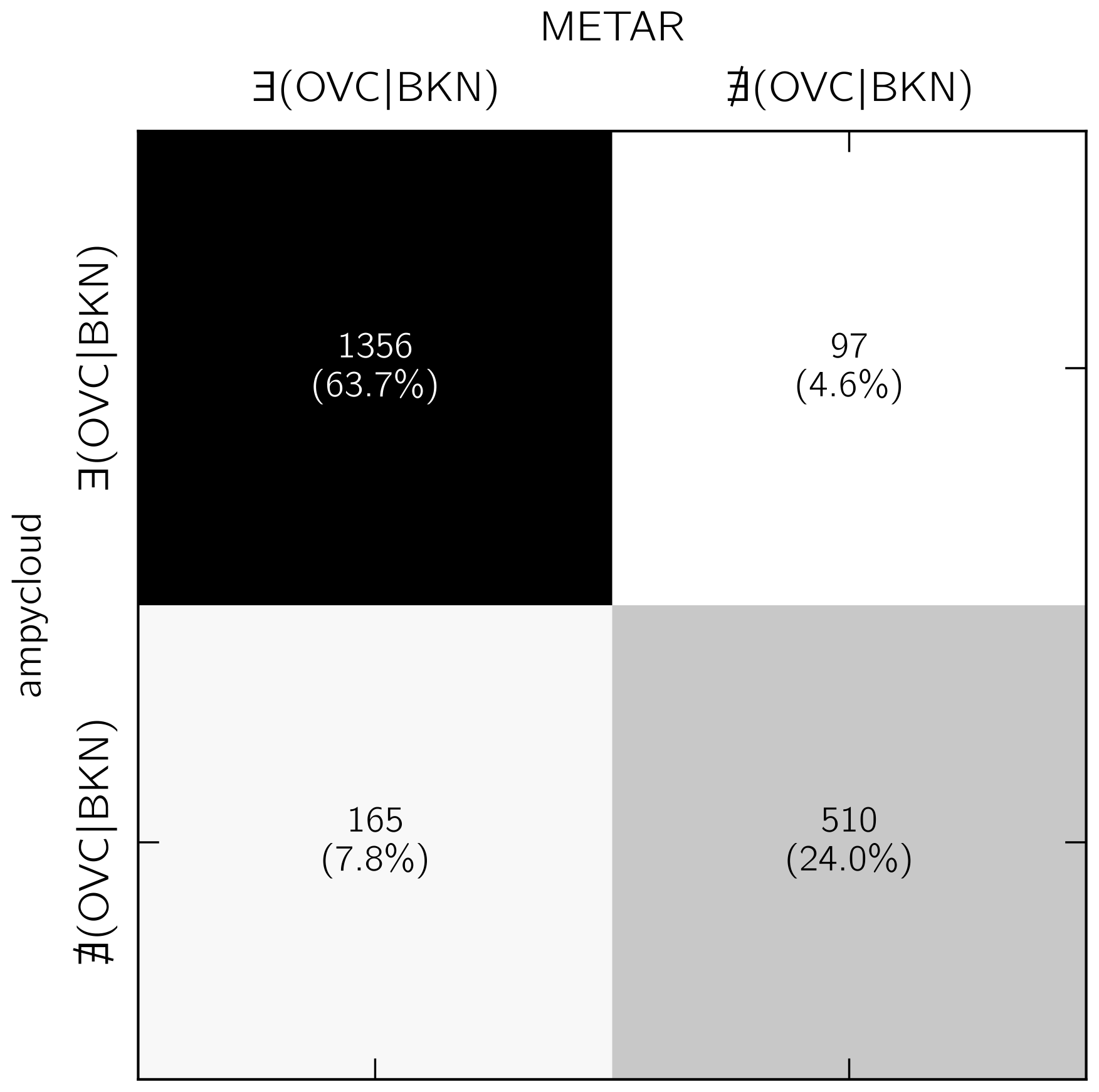
Figure 4Same as Fig. 3 but with simplified categories related to the presence or absence of a cloud ceiling.
The matrix in Fig. 3 is useful to identify cases with strong deviations in the sky coverage fraction. However, detecting the correct sky coverage fraction for a given cloud layer does not guarantee that the cloud layer will be detected at the correct height. We thus provide in Fig. 5a a comparison of the height of cloud layers with the highest sky coverage fractions measured by ampycloud with respect to those reported in the corresponding METAR. In 64.4 % of the cases, ampycloud identifies a cloud layer height that is in good agreement with the METAR. The majority of the remaining cases are comprised of situations where ampycloud provides somewhat lower cloud base heights than the METARs. This is a direct consequence of the conservative approach of the ampycloud algorithm, that considers the entire set of cloud and VV hits (in its default configuration) to derive a given cloud base height. The example in Fig. B11 illustrates this behavior. Cases in the bottom row (6.6 % of the total) correspond to situations where the cloud layer is missed entirely by the ceilometers over the duration of the time interval Δt.
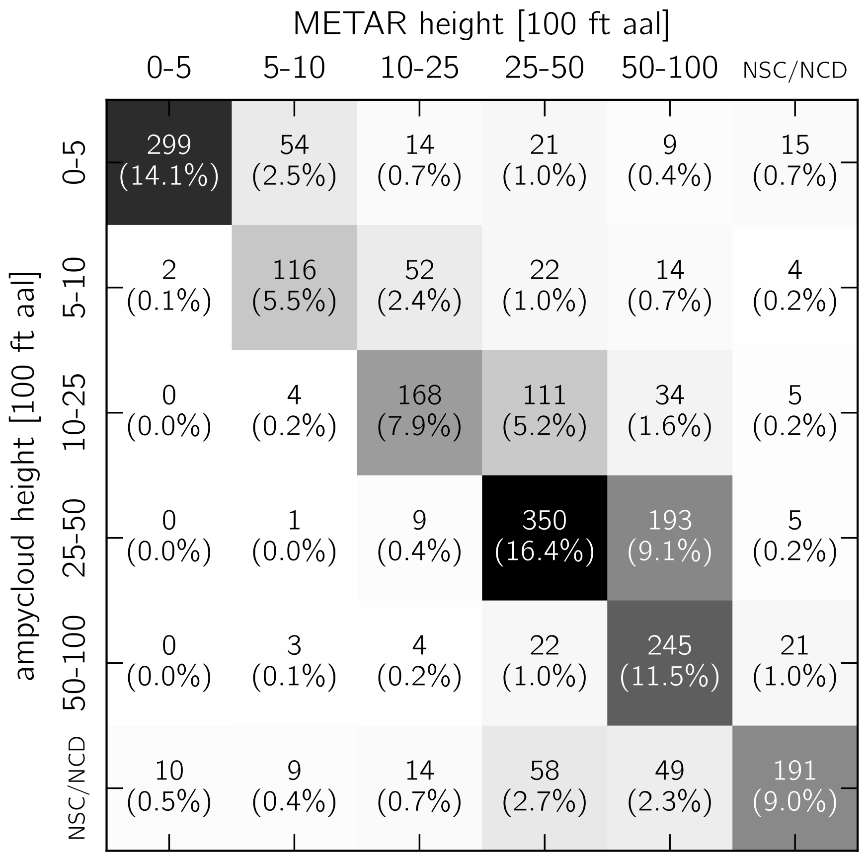
Figure 5Same as Fig. 3 but for the height of the densest cloud layer. The differences between ampycloud and the METARs are dominated by cases where ampycloud returns a cloud layer height somewhat lower than that of the METAR. This is a direct consequence of the conservative design of the algorithm that (in its default configuration) considers the entire look-back time to compute the height of a given set of cloud and VV hits.
The ampycloud Python package focuses tightly on the implementation of the ampycloud algorithm itself, with only a handful of dependencies, all well-maintained and under active development within the Python community. The ampycloud package is not designed to interact with the outside world (and other programming languages, e.g., via JSON format). The implementation of the necessary application programming interfaces (APIs) is left to the interested users. ampycloud is also not designed to handle partial or complete ceilometer failures or data transmission issues: it will simply process the cloud and VV hits that one feeds it. From this perspective, the handling of operational exceptions and errors must be done by the user before calling ampycloud.
In its current implementation, ampycloud uses a fixed time interval Δt to characterize cloud layers. In doing so, ampycloud is essentially trading-off its responsiveness to rapidly evolving conditions with its ability to obtain a more representative view of the entire sky. The default time interval Δt=15 min adopted by MeteoSwiss is shorter than in other algorithms with similar goals (see, e.g., Nadolski, 1998; Wauben, 2002; ICAO, 2011). However, unlike those algorithms that give additional weight to the most recent measurements, ampycloud treats every hit equally. This implies that ampycloud may possibly respond somewhat less rapidly to changes but should be more stable when analyzing sparse cloud layers. We note that increasing the value of Δt does not necessarily guarantee a better match with the AMOs. At LSGG, for example, there are often cumulus (humilis and/or mediocris, which are not operationally relevant) that remain stationary over the Jura mountain ridge and that can never be detected by the aerodrome's ceilometers. Several cases presented in Appendix B have the lowest cloud layer missed entirely by the ceilometers (see Figs. B4, B6, B7, B8, and B10). Had one used a time interval Δt=30 min instead of 15 min, the lowest cloud layers would still have been missed entirely by the ceilometers in each of these cases. Understanding the exact behavioral differences between ampycloud and other algorithms with similar purposes will require a dedicated comparison of their respective accuracies against a reference set of ceilometer data (either real or simulated), which is outside the scope of this article. Up until now, such comparisons were essentially impossible due to the private nature of source codes and the lack of detailed documentation. With this article and its accompanying material (Vogt, 2024), we purposely seek to make the ampycloud processing of the examples shown in Figs. B1 to B12 reproducible by motivated users and researchers.
It must be stressed that ampycloud does not challenge the quality or nature of the cloud and VV hits that it is being provided: it trusts them all fully and equally. The capacity of the algorithm to provide an accurate assessment of cloud layers above an aerodrome is thus directly limited by the ability of ceilometers to report clouds up to the aerodrome's MSA and to measure their heights accurately in the first place (Costa-Surós et al., 2013; Wagner and Kleiss, 2016; Kotthaus et al., 2016; Illingworth et al., 2019). This (current) reliance of ampycloud on cloud base hits (as reported by ceilometers via black-box algorithms) should not be overlooked by users interested in combining datasets from multiple ceilometer brands or models. Any spurious cloud hit (be it caused by measurement noise, rain, or airplanes flying overhead) will inevitably impact the outcome of ampycloud, as would a “lack of cloud hits”: for example, when the view towards upper layers is blocked by lower ones in complex situations. ampycloud does not do any upward correction of the cloud coverage of the upper layers (yet), e.g., as done in the ASOS algorithm (see, e.g., Appendix A, Sect. Cloud layers (8), Example 1 in ICAO, 2011). Another enhancement possibility for the ampycloud algorithm would be to use the wind speed to identify suitable look-back times as a function of height in order to obtain a (more) representative sampling of the sky. Doing so in real time could be achieved, at least up to the aerodrome minimum sector altitudes, by direct measurements (for example, using wind profilers), by data extraction from numerical models, or by a combination of both.
The slicing step of ampycloud relies on the rescaling factor τs to reduce the dimensionality of the 2-D clustering to almost 1-D. A further development might be to use a robust 1-D clustering method instead. The layering step of ampycloud is the part of the algorithm that shows the most potential for improvement for the following reasons. Unlike the slicing and grouping steps, the parameters γ and δ associated with this step are less directly related to physical quantities. For specific distributions of cloud hits, this step can be sensitive to the random seed used by the system6. Most importantly, the use of Gaussian mixture models clearly is not ideal from a physics perspective given the fact that cloud base hits are not expected (nor seen) to systematically follow a Gaussian distribution, although it remains a sufficiently valid approximation.
The main limitation of ampycloud, however, currently resides in the fact that it relies exclusively on cloud and VV hits, which are processed without question. The use of complete backscatter profiles from the ceilometers could help improve this state of affairs: for example, by enabling the identification of spurious hits triggered by heavy precipitation or aircraft and/or by supplementing cloud base height measurements with cloud layer thickness, which could significantly ease the identification of coherent structures. The use of complete backscatter profiles could also enable the identification of the maximum observed height (in the case of thick cloud layers) and better account for the sky coverage fraction of partially obscured cloud layers while removing any reliance on black-box algorithms (developed by ceilometer manufacturers to detect cloud base hits).
The use of a finite number of ceilometers alone cannot always be sufficient to differentiate very sparse cloud layers from a “true” clear sky. If a series of ceilometers detect no clouds, the use of pyrgeometers (see, e.g., Aviolat et al., 1998; Marty and Philipona, 2000; Dürr and Philipona, 2004), visible all-sky cameras (Wacker et al., 2015), infrared all-sky imagers (Aebi et al., 2018), or even satellite images could help in ascertaining the validity of a clear-sky condition – albeit without the ability to estimate the height of the sparse cloud layers that may have been missed by the ceilometers with the same accuracy. Similarly to Doppler lidars, the use of rotating-beam ceilometers (WMO, 2021) with the ability to probe more than one sightline could clearly improve the reliability of AUTO METARs for sparse cloud layers (i.e., for intermediate okta values), albeit at an increased financial cost and with maintenance challenges (a rotating mechanical component is more prone to technical issues).
The ampycloud algorithm was developed at MeteoSwiss as part of a large effort to fully automate the production of METARs at Swiss civil aerodromes. Its specific purpose is to determine the sky coverage fraction and base height of cloud layers using ceilometer data (in the form of individual cloud base hits). The eponymous Python package is released online as open-source software under the terms of the 3-Clause BSD license. The ampycloud Python package forms an integral part of the software infrastructure of MeteoSwiss. Yet, it does not contain any MeteoSwiss-specific code nor does it rely on any specific hardware–software infrastructure (all contained within the autometpy software suite; see Sect. 3.2). The code and its dedicated online (technical) documentation are completed by this article describing the underlying algorithm and its scientific motivation.
The accuracy of the ampycloud algorithm has been tested in detail on a series of specific examples (as illustrated in Figs. B1 to B12) and, statistically, over a reference set of cases extracted over a 5-year period. With the correct identification of a ceiling (or absence thereof) 87.7 % of the time, the results of the ampycloud algorithm are found to be in good agreement with the corresponding METARs, such that the use of this algorithm at LSGG was approved by the Swiss civil aviation authority.
The automatic production and dissemination of AUTO METARs without human supervision at LSGG started on 1 May 2024. Nonetheless, several elements of the ampycloud algorithm have potential for further improvement. The necessity and exact benefits of these improvements will be continuously investigated and evaluated by MeteoSwiss over the coming years throughout and beyond the transition from METAR to AUTO METAR at Swiss civil aerodromes.
The public release of ampycloud has taken place within a large paradigm change towards open government data in Switzerland (Assemblée fédérale de la Confédération suisse, 2023). An open-source software evidently facilitates additional testing of the algorithm at various locations beyond the Swiss civil aerodromes. Most importantly, we hope that it will ease the implementation of dedicated intercomparison campaigns to evaluate the accuracy of the various cloud algorithms deployed at aerodromes worldwide.
In ampycloud, Gaussian mixture models with one, two, and three components are used to determine whether a given group 𝒢 is comprised of multiple distinct sub-layers. To illustrate how the Bayesian information criterion (BIC) scores allow us to reliably select the optimal number of sub-layers in a given group, we create a series of artificial distributions of cloud hits. Each distribution is comprised of either two or three Gaussian layers, each with a number of randomly generated hits and with the layers being separated by height by up to Δ=8 times their standard deviation σ. Four examples of these distributions are presented in Fig. A1.
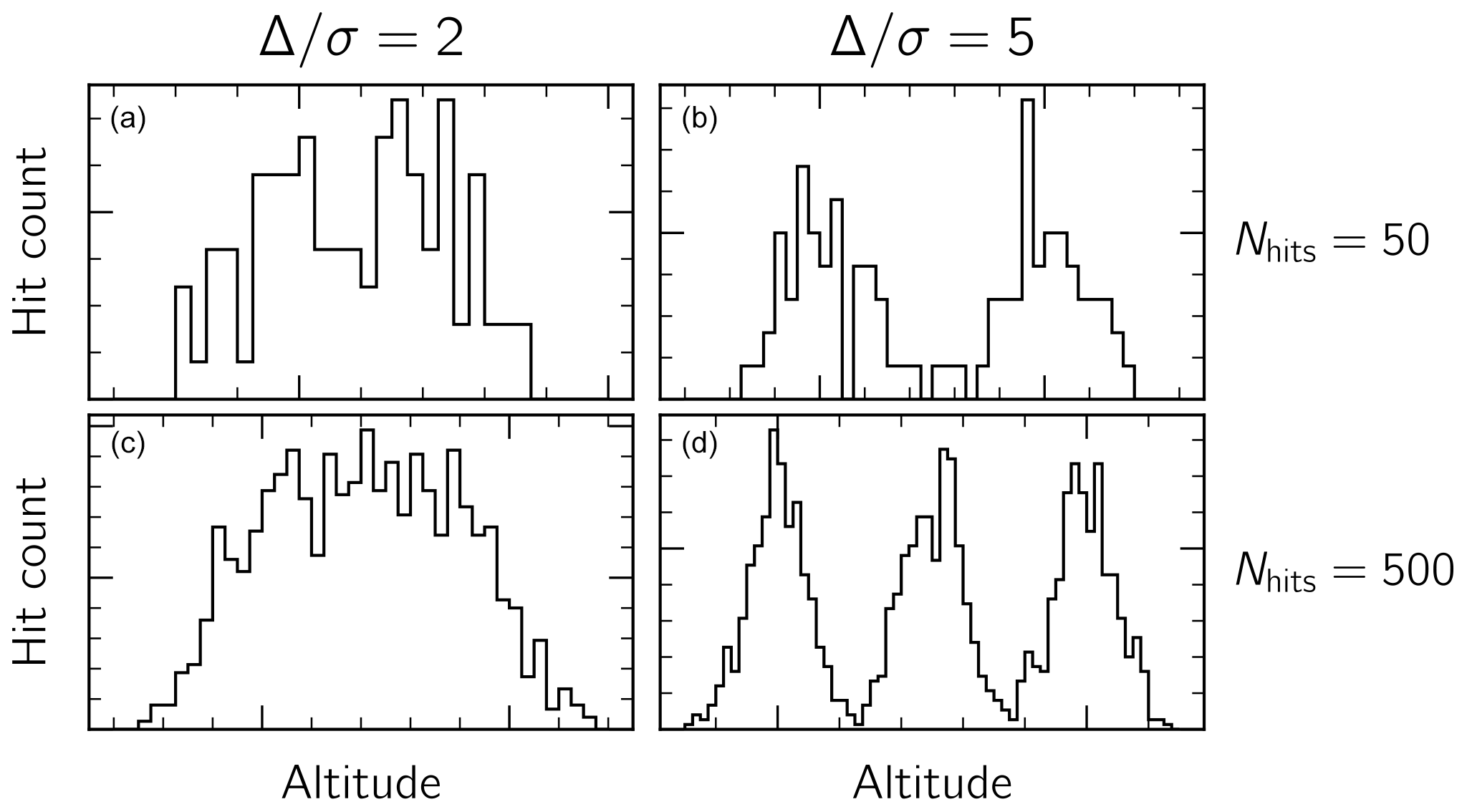
Figure A1Simulations of two (a, b) and three (c, d) cloud layers using random normal distributions with Nhits artificial cloud base hits per layer. Individual layers are separated by Δ=2 (a, c) and Δ=5 (b, d) standard deviations σ.
The Akaike information criterion (AIC) and Bayesian information criterion (BIC) scores provide means to assess the goodness of fit of different Gaussian mixture models. The smaller the AIC or BIC scores are, the better the model fit is. In ampycloud, we use BIC scores to decide whether a given group 𝒢 is composed of sub-layers. The AIC score tends to favor models with larger numbers of components, which is at odds with the ampycloud approach of favoring – for near-equal scores – the lowest number of Gaussian components to prevent unjustified sub-layering. Therefore, we rely on the BIC score only.
The relative likelihood of different Gaussian mixture models can be used to assign probabilities to each of them. The Bayesian probability of model i is
with BICmin being the minimum BIC score among the Gaussian mixture models under consideration.
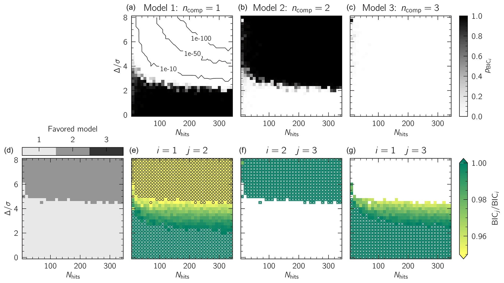
Figure A2Illustration of the ability of the ampycloud layering step to distinguish the presence of two simulated Gaussian sub-layers inside a group 𝒢 as a function of the relative separation of the sub-layers Δ (expressed in terms of the layers' standard deviation σ) and the number of cloud hits per layer Nhits. (a–c) BIC probabilities pBIC computed following Eq. (A1), built from the relative likelihood of Gaussian mixture models with one (a), two (b), and three (c) components. Each pixel in the image corresponds to the median of 10 independent realizations. For very low numbers of hits per layer (Nhits≲50), the selection of the best Gaussian mixture model is less sharp. When the sub-layers are close to one another (with Δ≲2σ), the Gaussian mixture model approach is unable to reliably identify two distinct components. (e–g) Distributions of BICj / BICi for the cases of one component vs. two, two components versus three, and one component versus three. For the cases where BICj / BICi>1 are tagged with a white cross, these are regions where the model with j components is unambiguously rejected against the model with i components because of a larger BIC score. On the other hand, for the cases where BICj / BICi<0.95 are tagged using black circles, and for these only, ampycloud will favor the model with j components following Eq. (A2). The resulting map of the model favored by ampycloud as a function of Nhits and is visible in the bottom-left diagram (d).
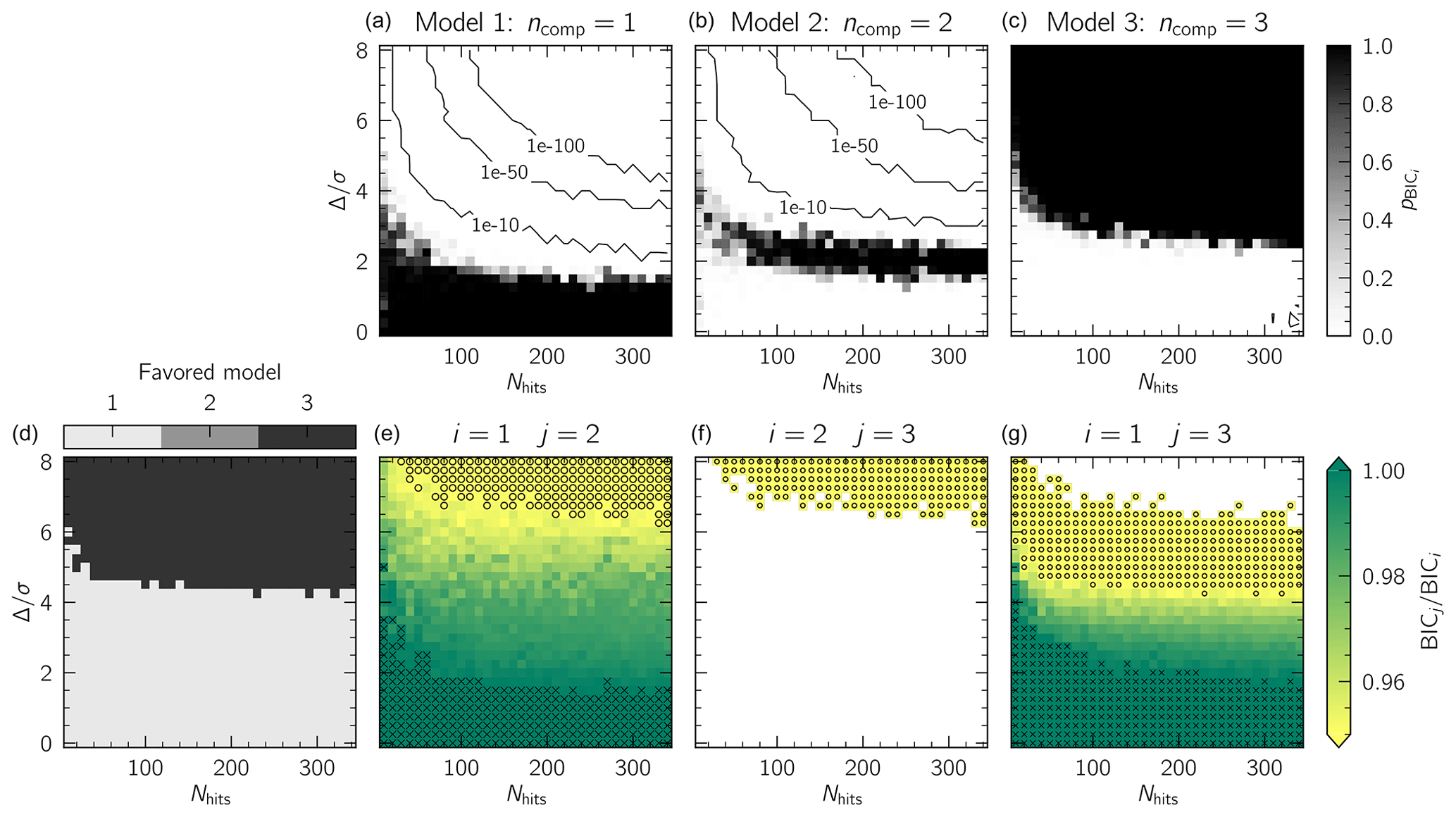
Figure A3Same as Fig. A2 but for three simulated layers. As for the case of two simulated layers, the ampycloud layering step is able to correctly identify three distinct layers when they are separated by ∼5 standard deviations (Δ≳5σ). A single layer is favored otherwise.
We show in Fig. A2 the values of pBIC,i for the simulated datasets with two Gaussian sub-layers. The Gaussian mixture model approach appears to be incapable of identifying two distinct components when Δ≲2σ, i.e., when the layers are separated by less than twice their standard deviation. For cases with Δ≳2σ, the probability of the distributions being comprised of a single Gaussian distribution drops extremely rapidly in favor of the two-component model. The transition is slightly less sharp for cases with a lower number of cloud base hits (i.e., cases where Nhits≲50). The case of three simulated cloud layers is shown in Fig. A3. A single component is favored by the Gaussian mixture model approach for cases where Δ≲2σ. A narrow, intermediate zone favoring two components is present for cases where , whereas three components are correctly identified for cases where Δ≳3σ.
Unlike the simulated cases presented here, real cloud base hits do not follow a Gaussian distribution, particularly due to temporal trends in the cloud base heights (a fact which is clearly visible in Figs. B1 to B8). For real cases, using the probabilities pBIC to select the optimal number of sub-layers present inside a given group 𝒢 works too efficiently in the sense that a single Gaussian component is ruled out too rapidly in the case of broad, flat layers. To circumvent this limitation, ampycloud uses a slightly adjusted selection criterion based on the BIC scores which varies more smoothly as a function of the (normalized) layer separation . The general idea is to assume that one component is present and to only favor a solution with two (or three) components if the decrease in the associated BIC scores is sufficiently significant. In other words, a model with j components is favored over a model with i components only if
where δ is a multiplicative factor (a parameter of the ampycloud algorithm).
The consequences of these selection criteria are shown in the bottom rows of Figs. A2 and A3. Varying the value of δ allows us to more easily decide the level at which two (or three) components are favored over a single one. With the default ampycloud value of δ=0.95, this transition occurs at . Sub-layers are therefore identified in a given group 𝒢 only if they are well separated, as illustrated in Fig. A1. For the case of three simulated sub-layers, the selection criterion defined in Eq. (A2) also has the advantage that it never favors two components (unlike the probabilities pBIC, as illustrated in Fig. A2). If three components cannot be identified unambiguously, no sub-layering occurs.
We present in Figs. B1 to B12 the ampycloud diagnostic diagrams from a series of representative, real situations taken from the LSGG and LSZH aerodromes. These examples serve to illustrate the behavior of ampycloud in different conditions and to compare the algorithm's output with the official METAR cloud codes that were validated and issued by an AMO at the time. For the ease of readability, each example is discussed in detail in the associated figure caption. These examples are all part of the set of cases used to verify the scientific behavior of the ampycloud algorithm over the course of its development by means of dedicated tests (ampycloud, 2024c) run using the pytest module.
The underlying sets of cloud and VV hits associated with each example are made available to the interested reader, alongside a small Python script designed to process them using ampycloud and to generate the associated ampycloud diagnostic diagrams. This material is archived on Zenodo and is publicly available (under a Creative Commons Attribution 4.0 International license; Vogt, 2024).
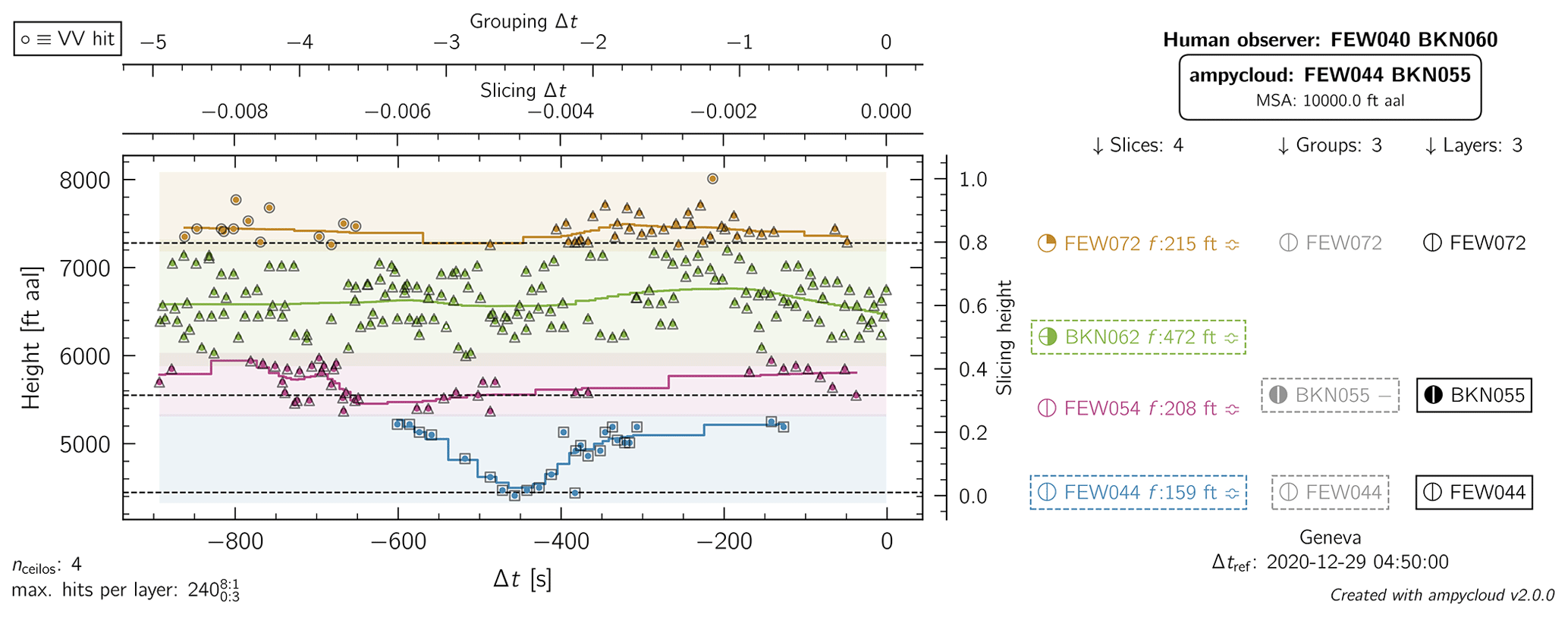
Figure B1ampycloud diagnostic diagram for LSGG on 29 December 2020 at 04:50 UTC. The hits from four ceilometers over a period of 15 min are being considered. The four dominant slices are found to be overlapping, but the separations between individual hits is too large for the second processing step to bundle them all into a common master group. The symbol − in the “groups” column on the right-hand side indicates that sub-layers are being searched for (but not found) by the layering step for the second group (from bottom; BKN055), which is the only structure with sufficient hits to do so (i.e., with a sky coverage fraction larger than or equal to 2 oktas).
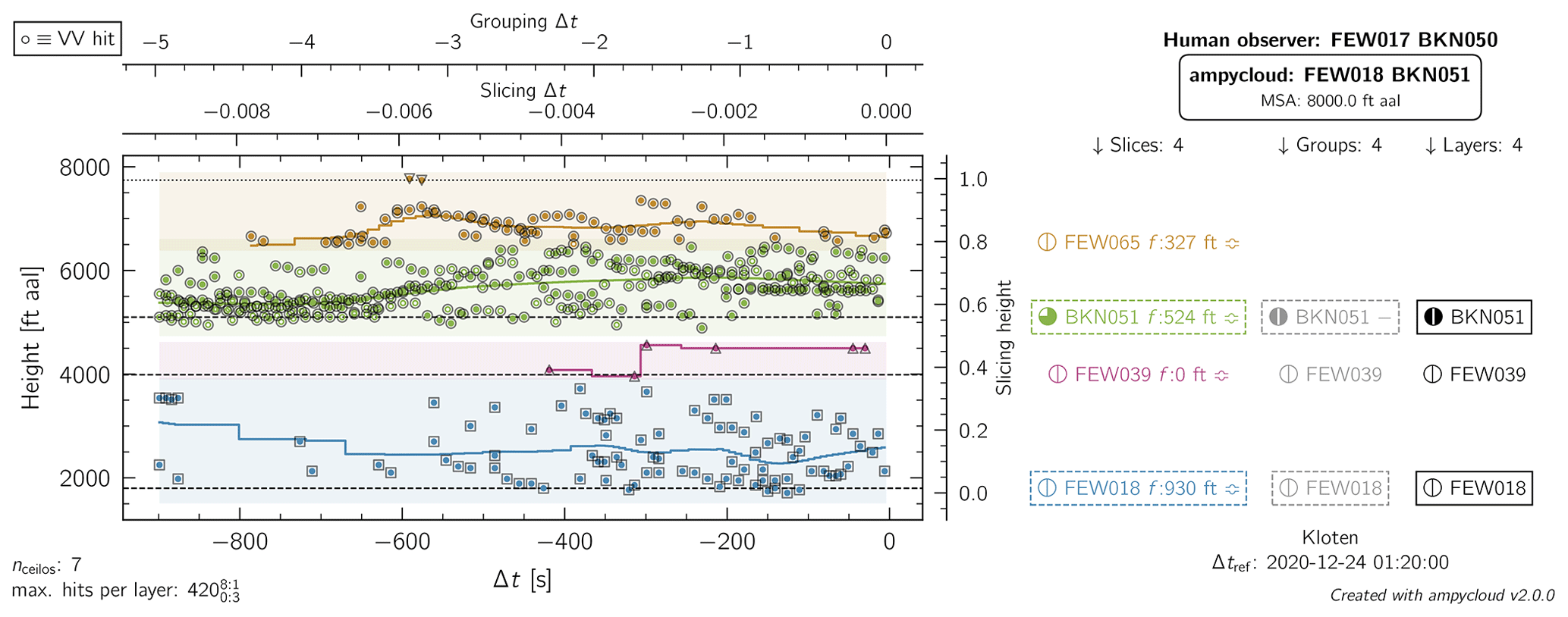
Figure B2Same as Fig. B1 but for LSZH on 24 December 2020 at 01:20 UTC. VV hits are indicated using colored points with no filling: they are treated like regular cloud base hits by ampycloud. In this example, the grouping step has been used to merge the majority of hits in the top two slices: only the highest two cloud base hits remain as the upper-most layer, but they are discarded as a minimum of four hits are required for a layer to be considered to have a sky coverage fraction above 0 oktas (i.e., Θ0=3).
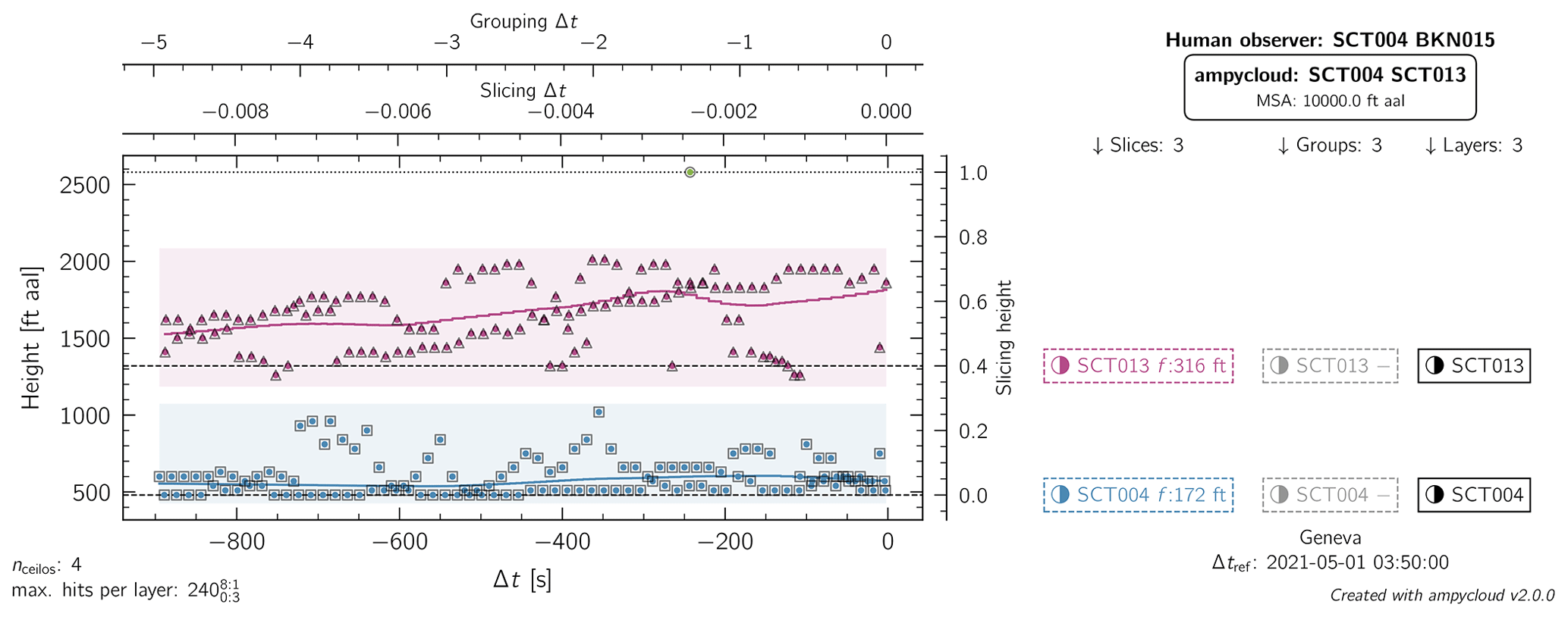
Figure B3Same as Fig. B1 but for LSGG on 1 May 2021 at 03:50 UTC. In this case, the slicing step correctly identifies the two dominant cloud layers present. The grouping and layering steps do not modify the initial slices. The top SCT013 layer slightly underestimates the sky coverage fraction that was reported to be BKN by the AMO, plausibly because of its obscuration by the lower layer.
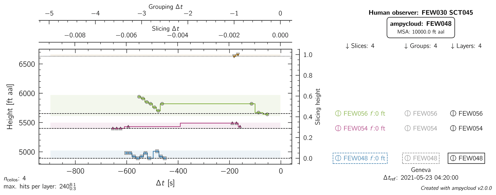
Figure B4Same as Fig. B1 but for LSGG on 23 May 2021 at 04:20 UTC. In this case, with very sparse layers, the slicing step correctly identifies the dominant cloud layers present. The layer at 3000 ft reported by the observer is missed entirely by the ceilometers over the duration of the time interval Δt=900 s, while the sky coverage fraction of the layer at 4500–4800 ft is slightly underestimated by the ceilometers. Should a user prefer a less granular output at high altitudes, it is sufficient to change the parameters Δhl,vals and Δhl,lims to set a minimum separation value of 500 ft above 5000 ft, for example.
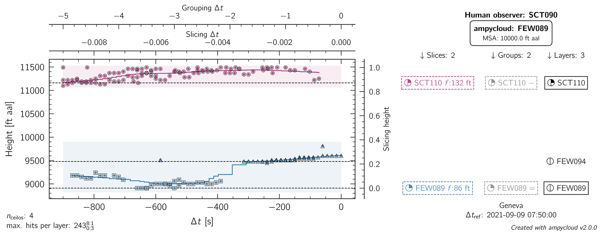
Figure B5Same as Fig. B1 but for LSGG on 9 September 2021 at 07:50 UTC. The ampycloud layering step identifies two sub-layers separated by ∼500 ft in the bottom group, with a sky coverage fraction of FEW smaller than the SCT090 reported by the AMO, who likely merged the two sub-layers together. It is, however, worth noting that even the group FEW089 identified by ampycloud (bottom entry of the middle column) does not reach a sky coverage fraction of SCT, indicating that the ceilometers were globally looking at clear sightlines. The top layer SCT110 detected by ampycloud is not reported in the view of the MSA applicable at LSGG.
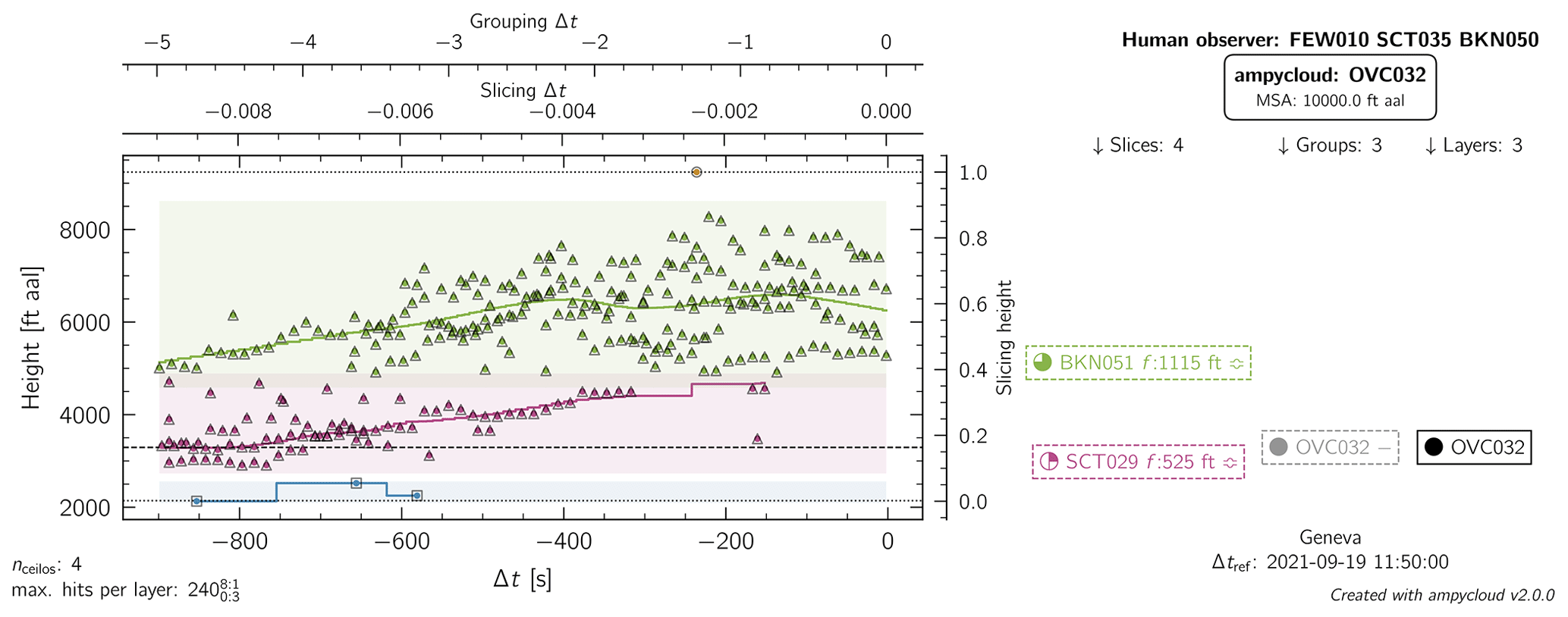
Figure B6Same as Fig. B1 but for LSGG on 19 September 2021 at 11:50 UTC. The AMO reported two distinct layers at 3500 and 5000 ft, which is consistent with the initial ampycloud slices. The overall cloud hit distribution is, however, suggestive of a single coherent structure increasing from 3000 to 5000 ft over the 15 min interval and is identified as such by the grouping step of the ampycloud algorithm. The bottom layer at 1000 ft is missed entirely by the ceilometers over the duration of the time interval Δt=900 s.
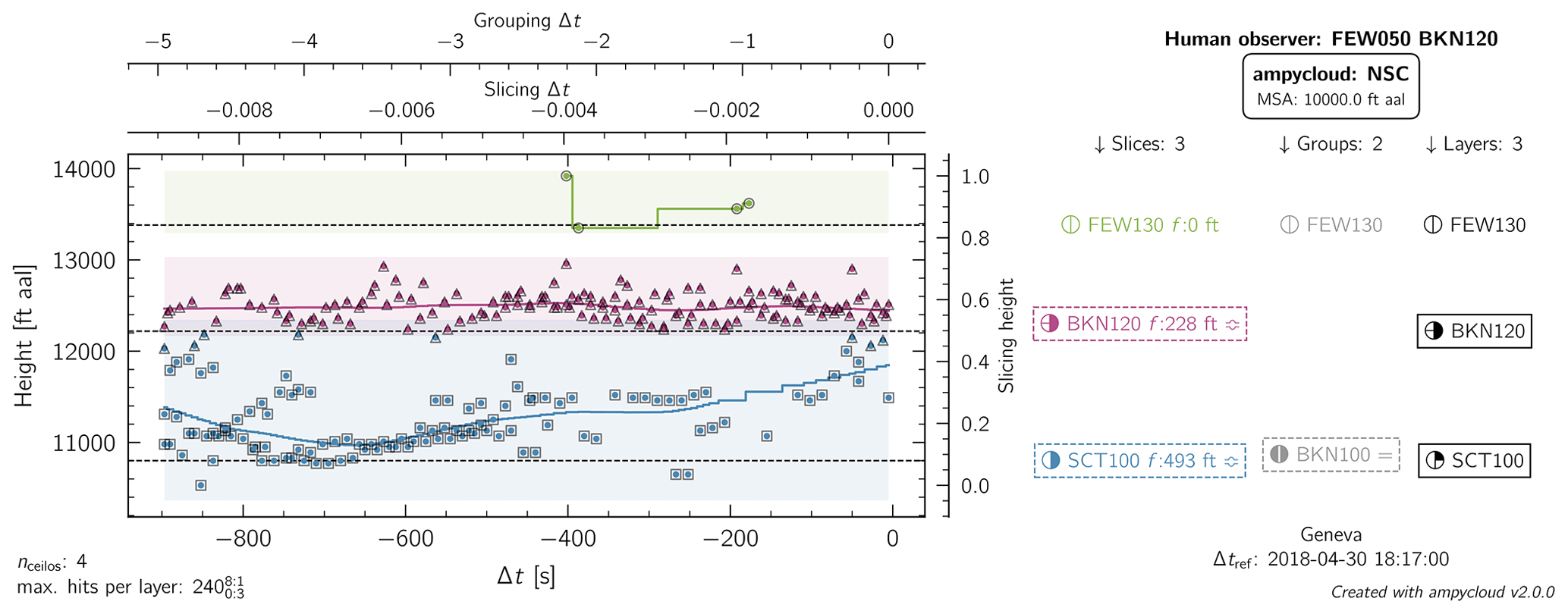
Figure B7Same as Fig. B1 but for LSGG on 30 April 2018 at 18:17 UTC. The value of ΔMSA is exceptionally set to 4000 ft in this example for visualization purposes. The bottom two slices are merged into a single structure by the grouping step (as they connect to each other at the start and end of the interval) and are then re-separated into two distinct layers. Clouds at 5000 ft were missed entirely by the ceilometers over the duration of the time interval Δt=900 s. This example also illustrates the difficulty in blindly comparing METARs with AUTO METARs. The AMO decided to report the BKN120 layer despite the MSA applicable at LSGG (whereas ampycloud simply ignores it), leading to an (apparently) missed ceiling.
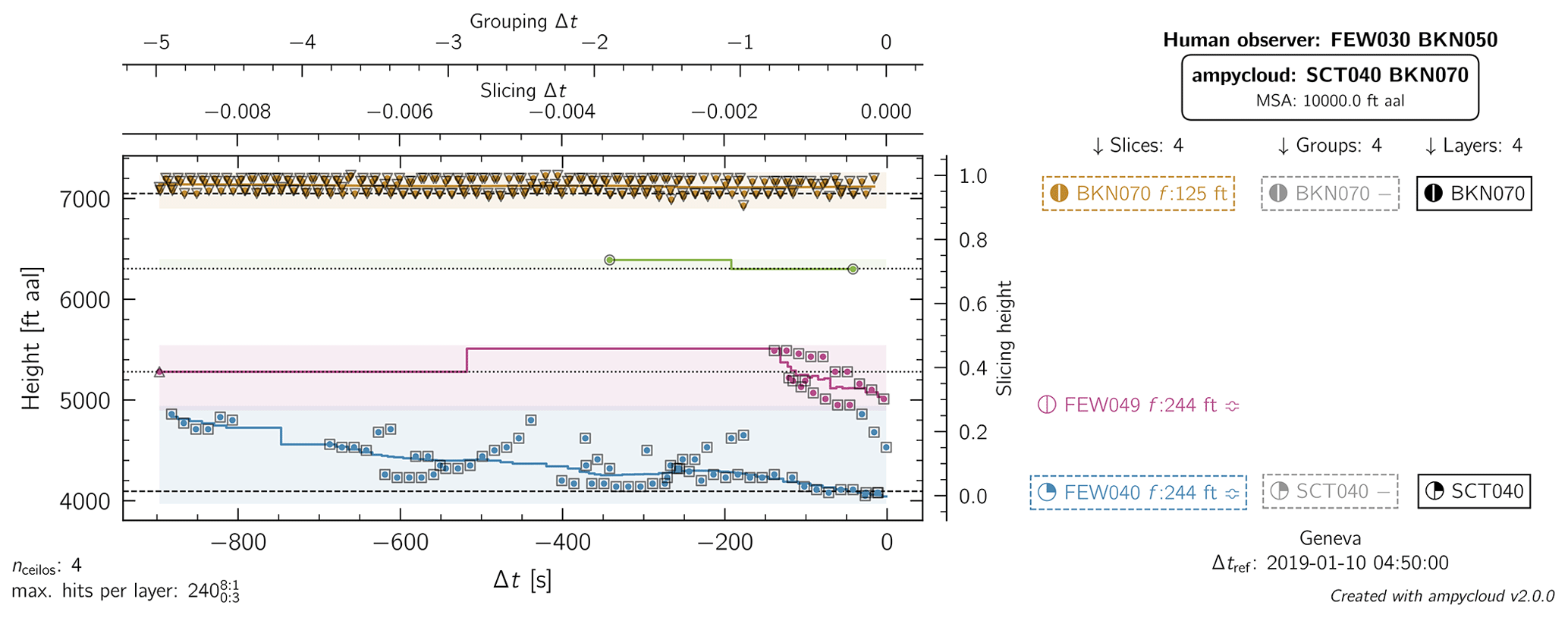
Figure B8Same as Fig. B1 but for LSGG on 10 January 2019 at 04:50 UTC. It is because ampycloud accounts for the fluffiness of the bottom two slices that the grouping step decides that these form a single structure despite the somewhat offset cluster of hits appearing within the last 150 s. It is not clear why the layer at 7000 ft was not reported in the METAR while clouds at 3000 ft were missed entirely by the ceilometers over the duration of the time interval Δt=900 s.
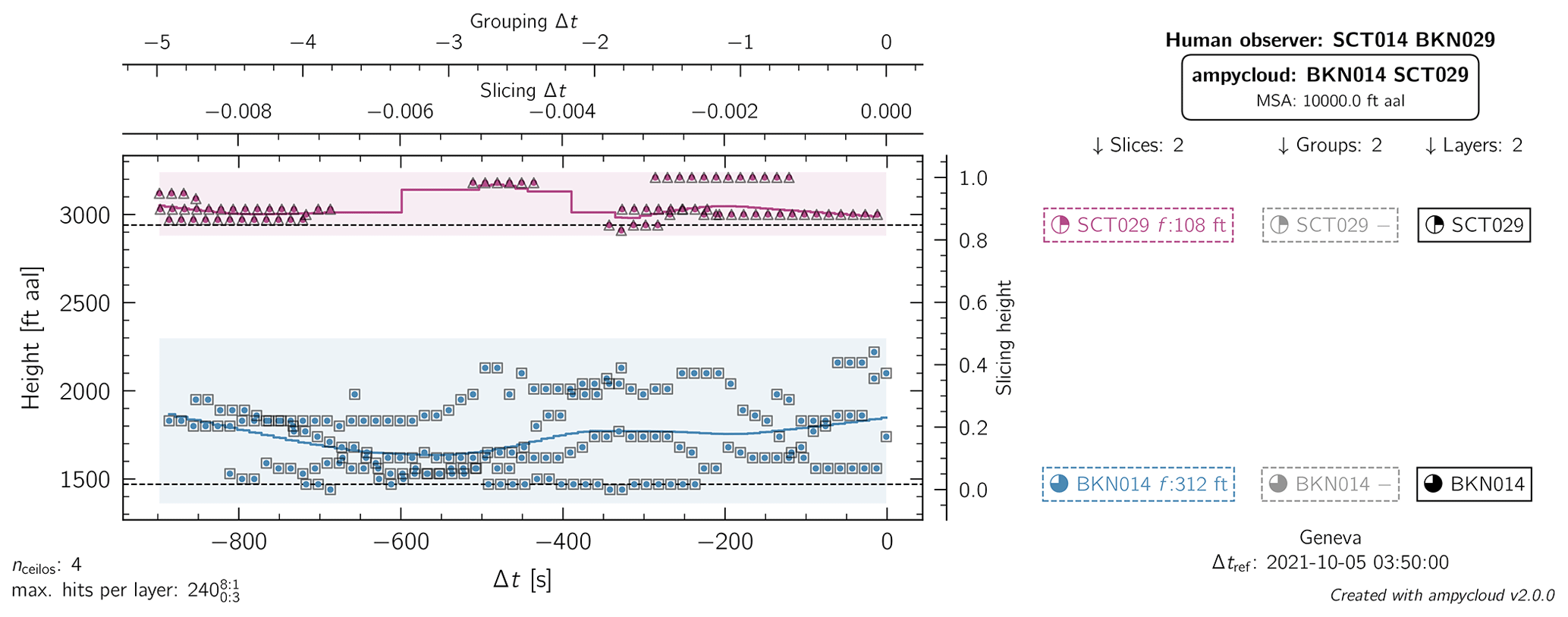
Figure B9Same as Fig. B1 but for LSGG on 5 October 2021 at 03:50 UTC. The slicing step correctly identifies the two cloud layers present, albeit with a slightly different sky coverage fraction than that reported by the AMO. The top group is not separated into two distinct sub-layers by the layering step because their separation of ∼180 ft would be smaller than the minimum value of ft.
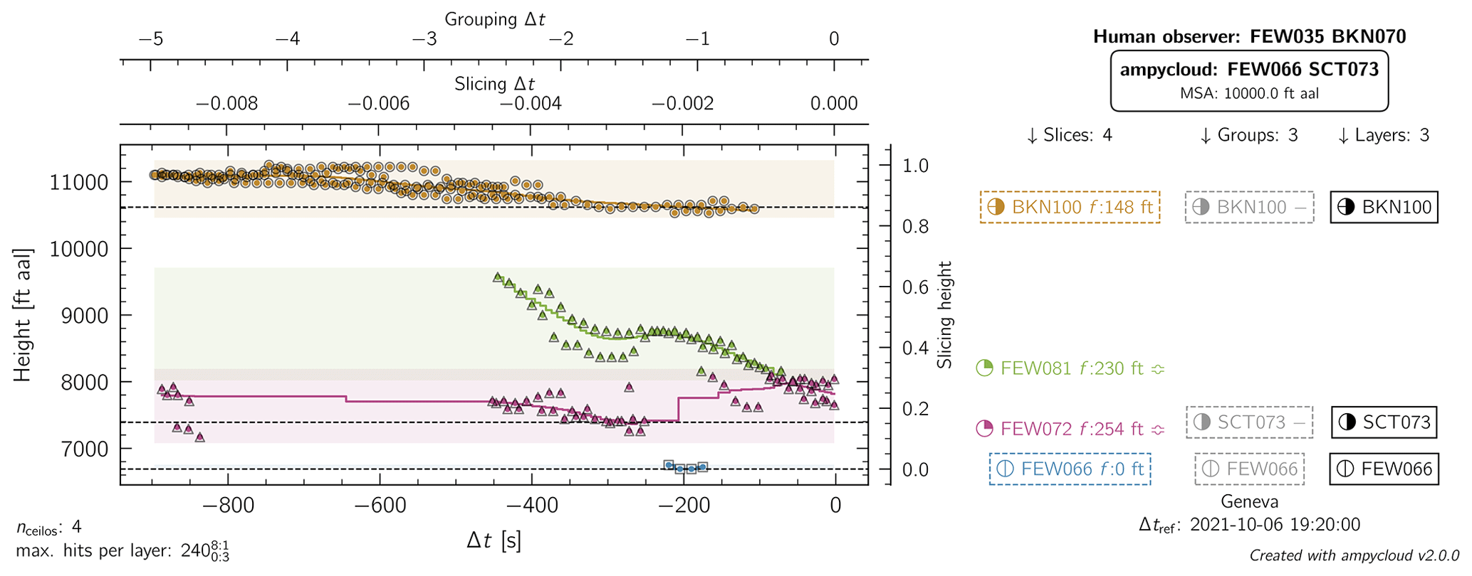
Figure B10Same as Fig. B1 but for LSGG on 6 October 2021 at 19:20 UTC. The grouping step is key to connect the two central slices given the rapidly decreasing nature of the cloud base between −400 and −100 s. Once again, the layer FEW035 reported by the AMO is missed entirely by the ceilometers over the duration of the time interval Δt=900 s.
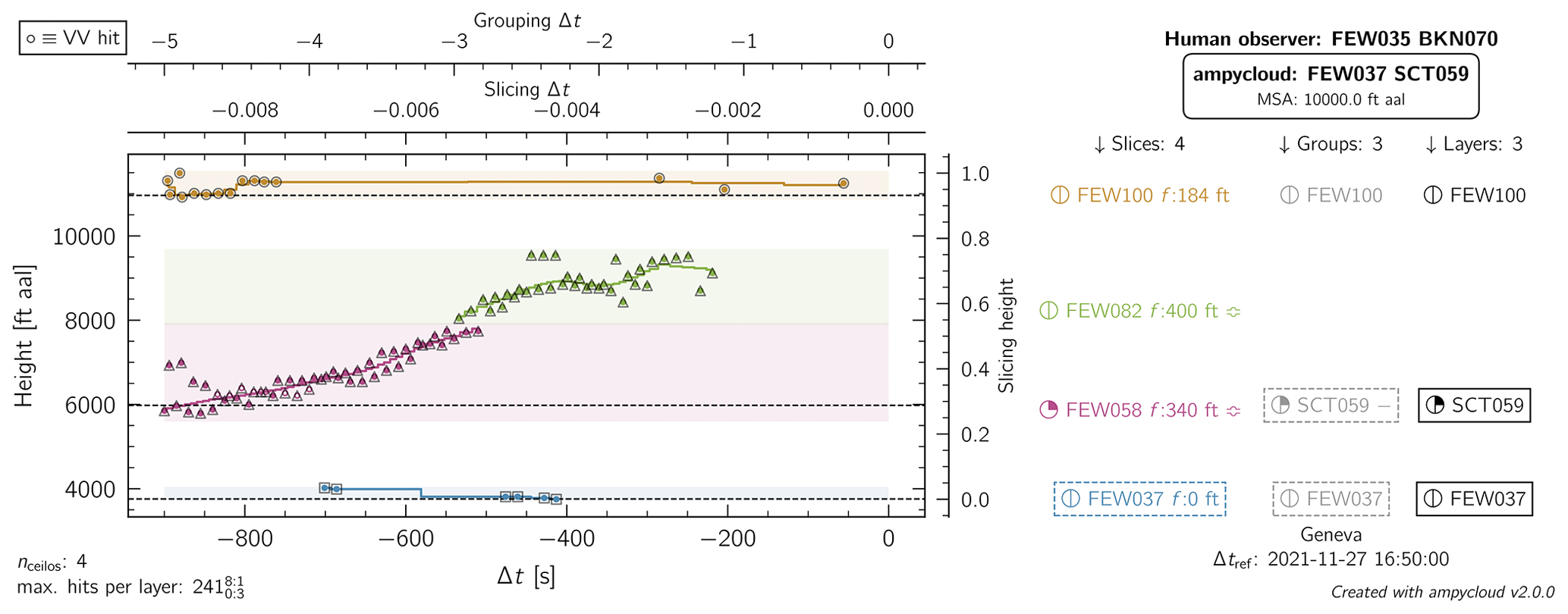
Figure B11Same as Fig. B1 but for LSGG on 27 November 2021 at 16:50 UTC. The grouping step correctly joins the middle two slices in this case with a rapidly rising cloud base. ampycloud considers the full set of hits (with βt=100 % by default) to derive the base height of this layer, whereas the AMO is likely to have ignored the oldest ceilometer data.
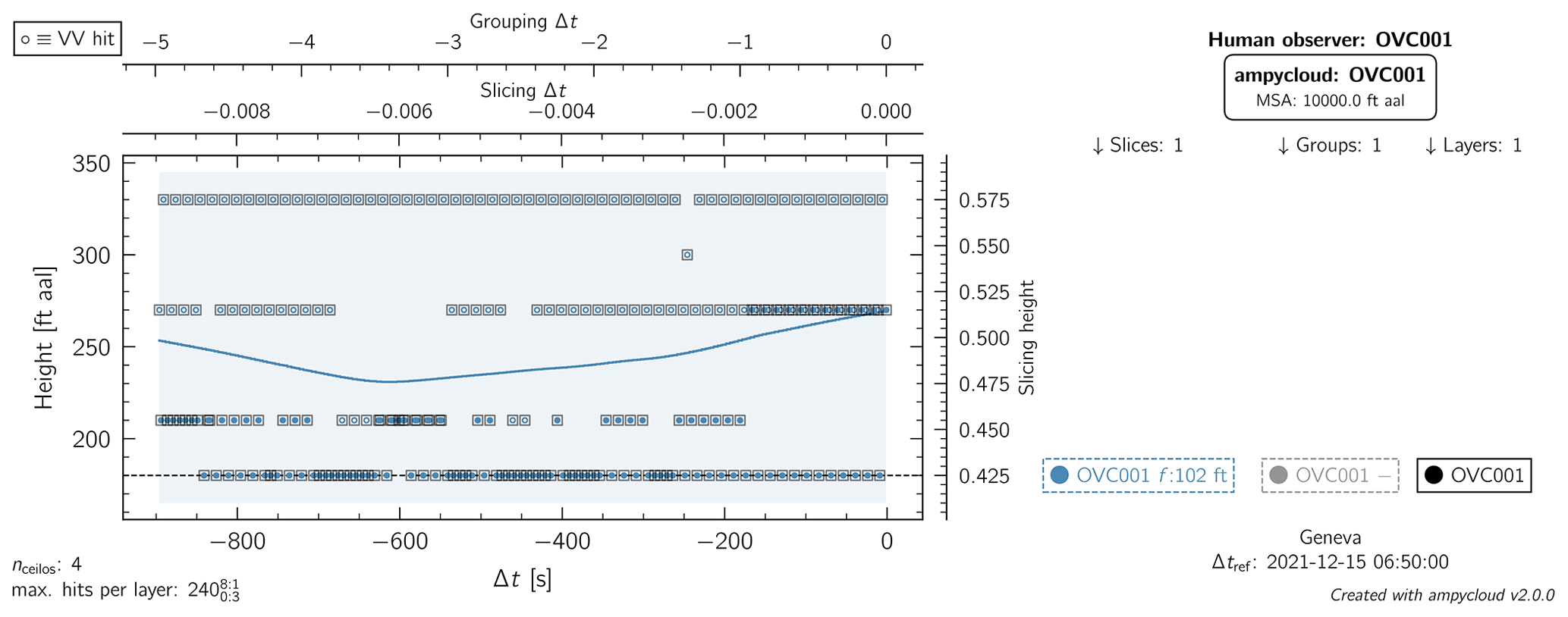
Figure B12Same as Fig. B1 but for LSGG on 15 December 2021 at 06:50 UTC. A single OVC001 slice is (correctly) identified by the ampycloud algorithm in this case, with a large number of VV hits being reported by the ceilometers. However, we stress once again that ampycloud is neither intended nor designed to formally decide whether a VV code must be issued in the AUTO METAR (instead of OVC001 in this example). This task should be performed by a separate algorithm focusing on vertical-visibility detection and reporting.
The ampycloud Python package is freely available on GitHub (https://github.com/MeteoSwiss/ampycloud, last access: 1 July 2024), with each release archived on Zenodo (DOI: https://doi.org/10.5281/zenodo.8399683, Vogt et al., 2024). The script and cloud hits used to generate the figures in Appendix B have also been stored on Zenodo (DOI: https://doi.org/10.5281/zenodo.10171151, Vogt, 2024), from where they can be downloaded freely. Diagrams in this article have been generated using the ampycloud Python module, which relies on the following Python packages: matplotlib (https://doi.org/10.5281/zenodo.592536, The Matplotlib Development Team, 2024; Hunter, 2007), NumPy (https://github.com/numpy/numpy/, Harris et al., 2020), Pandas (https://doi.org/10.5281/zenodo.4452601, The Pandas Development Team, 2021; McKinney, 2010), scikit-learn (https://doi.org/10.5281/zenodo.591564, Grisel et al., 2024; Pedregosa et al., 2011), SciPy (https://doi.org/10.5281/zenodo.595738, Gommers et al., 2024; Virtanen et al., 2020), and statsmodels (https://doi.org/10.5281/zenodo.593847, Perktold et al., 2024; Seabold and Perktold, 2010). The ampycloud diagrams were enhanced using the metsymb LaTeX package (https://doi.org/10.5281/zenodo.8302082, Vogt, 2023).
The ampycloud algorithm was designed by FPAV, with inputs from LF and DR. The ampycloud Python package was assembled by FPAV with important contributions from DR, LF, SR, and NTB and feedback from MB, PJ, SB, TH, PdP, and DF. The large-scale statistical assessment of the code was performed by DR, with contributions from LF, MB, and NTB. All the authors contributed to the writing of this article.
The contact author has declared that none of the authors has any competing interests.
Publisher's note: Copernicus Publications remains neutral with regard to jurisdictional claims made in the text, published maps, institutional affiliations, or any other geographical representation in this paper. While Copernicus Publications makes every effort to include appropriate place names, the final responsibility lies with the authors.
We thank Kenneth Boutin and Chet Schmitt for sharing with us the detailed description of the latest sky condition algorithm used by NOAA's ASOS program. We are grateful to the two anonymous reviewers and Peter Kuma for their feedback, which allowed us to improve this article in several parts.
This paper was edited by André Ehrlich and reviewed by Peter Kuma and two anonymous referees.
Aebi, C., Gröbner, J., and Kämpfer, N.: Cloud fraction determined by thermal infrared and visible all-sky cameras, Atmos. Meas. Tech., 11, 5549–5563, https://doi.org/10.5194/amt-11-5549-2018, 2018. a
ampycloud: Ampycloud Github Repository, https://github.com/MeteoSwiss/ampycloud (last access: 1 July 2024), 2024a. a
ampycloud: Ampycloud Online Documentation, https://meteoswiss.github.io/ampycloud (last access: 1 July 2024), 2024b. a, b
ampycloud: Ampycloud Scientific Stability Tests, https://github.com/MeteoSwiss/ampycloud/blob/develop/test/ampycloud/test_scientific_stability.py (last access: 1 July 2024), 2024c. a
ampycloud: Ampycloud Speed Test Action, https://github.com/MeteoSwiss/ampycloud/actions/workflows/CI_speed_check.yml (last access: 1 July 2024), 2024d. a
ampycloud: Ampycloud Speed Test Result, https://meteoswiss.github.io/ampycloud/installation.html#testing-the-installation-speed-benchmark (last access: 1 July 2024), 2024e. a
Assemblée fédérale de la Confédération suisse: Loi fédérale sur l'utilisation de moyens électroniques pour l'exécution des tâches des autorités, https://www.fedlex.admin.ch/eli/fga/2023/787/fr (last access: 1 July 2024), 2023. a
Aviolat, F., Cornu, T., and Cattani, D.: Automatic Clouds Observation Improved by an Artificial Neural Network, J. Atmos. Ocean. Tech., 15, 114–126, https://doi.org/10.1175/1520-0426(1998)015<0114:ACOIBA>2.0.CO;2, 1998. a
Boers, R., de Haij, M. J., Wauben, W. M. F., Baltink, H. K., van Ulft, L. H., Savenije, M., and Long, C. N.: Optimized Fractional Cloudiness Determination from Five Ground-Based Remote Sensing Techniques, J. Geophys. Res.-Atmos., 115, D24116, https://doi.org/10.1029/2010JD014661, 2010. a, b
Campbell Scientific: SkyVUE PRO (CS135) LIDAR Ceilometer, Product Manual, Tech. rep., Campbell Scientific, Inc., 2021. a
Cleveland, W. S.: Robust Locally Weighted Regression and Smoothing Scatterplots, J. Am. Stat. Assoc., 74, 829–836, https://doi.org/10.1080/01621459.1979.10481038, 1979. a
Costa-Surós, M., Calbó, J., González, J. A., and Martin-Vide, J.: Behavior of Cloud Base Height from Ceilometer Measurements, Atmos. Res., 127, 64–76, https://doi.org/10.1016/j.atmosres.2013.02.005, 2013. a
de Haij, M., Apituley, A., Koestse, W., and Bloemink, H.: Transition towards a New Ceilometer Network in the Netherlands: Challenges and Experiences, in: TECO-2016 – WMO Technical Conference on Meteorological and Environmental Instruments and Methods of Observations, 27–30 September 2016, Madrid, Spain, Instruments and Observing Methods Report No. 125, World Meteorological Organization (WMO), Madrid, Spain, 2016. a
Denby, L., Böing, S. J., Parker, D. J., Ross, A. N., and Tobias, S. M.: Characterising the Shape, Size, and Orientation of Cloud-Feeding Coherent Boundary-Layer Structures, Q. J. Roy. Meteor. Soc., 148, 499–519, https://doi.org/10.1002/qj.4217, 2022. a
Dürr, B. and Philipona, R.: Automatic Cloud Amount Detection by Surface Longwave Downward Radiation Measurements, J. Geophys. Res.-Atmos., 109, D05201, https://doi.org/10.1029/2003JD004182, 2004. a
Gommers, R., Virtanen, P., Haberland, M., Burovski, E., Weckesser, W., Reddy, T., Oliphant, T. E., Cournapeau, D., Nelson, A., alexbrc, Roy, P., Peterson, P., Polat, I., Wilson, J., endolith, Mayorov, N., van der Walt, S., Brett, M., Laxalde, D., Larson, E., Sakai, A., Millman, J., Colley, L., Lars, peterbell10, Carey, C. J., van Mulbregt, P., Bowhay, J., eric-jones, and Striega, K.: scipy/scipy: SciPy 1.14.1 (v1.14.1), Zenodo [code], https://doi.org/10.5281/zenodo.595738, 2024. a
Görsdorf, U., Mattis, I., Pittke, G., Bravo-Aranda, J. A., Brettl, M., Cermak, J., Drouin, M.-A., Geiß, A., Haefele, A., Haefelin, M., Hervo, M., Kominkova, K., Leinweber, R., Lehmann, V., Müller, G., Münkel, C., Pattantyus-Abraham, M., Pönitz, K., Wagner, F., and Wiegner, M.: The Ceilometer Inter-Comparison Campaign CeiLinEx2015 – Cloud Detection and Cloud Base Height, in: Technical Conference on Meteorological and Environmental Instruments and Methods of Observation (TECO), 27–30 September 2016, Madrid, Spain, World Meteorological Organization (WMO), 2016. a
Görsdorf, U., Klaus, D., Dhillon, R. S., Vande Hey, J. D., Lange, I., and Lehmann, V.: Efforts to Develop a Quantitative Definition of Cloud Base Height for Aviation, in: Technical Conference on Meteorological and Environmental Instruments and Methods of Observation (TECO), 8–16 October 2018, Amsterdam, the Netherlands, World Meteorological Organization (WMO), 2018. a
Grisel, O., Mueller, A., Lars, Gramfort, A., Louppe, G., Fan, T. J., Prettenhofer, P., Blondel, M., Niculae, V., Nothman, J., Lemaitre, G., Joly, A., Estève, L., du Boisberranger, J., Vanderplas, J., Kumar, M., Qin, H., Hug, N., Jalali, A., Varoquaux, N., Layton, R., Raghav, R., Schönberger, J., Liu, L., Jerphanion, J., Yurchak, R., Lorentzen, C., Dupré la Tour, T., Li, W., and Marmo, C.: scikit-learn/scikit-learn: Scikit-learn 1.5.1 (1.5.1), Zenodo [code], https://doi.org/10.5281/zenodo.591564, 2024. a
Harris, C. R., Millman, K. J., van der Walt, S. J., Gommers, R., Virtanen, P., Cournapeau, D., Wieser, E., Taylor, J., Berg, S., Smith, N. J., Kern, R., Picus, M., Hoyer, S., van Kerkwijk, M. H., Brett, M., Haldane, A., del Río, J. F., Wiebe, M., Peterson, P., Gérard-Marchant, P., Sheppard, K., Reddy, T., Weckesser, W., Abbasi, H., Gohlke, C., and Oliphant, T. E.: Array Programming with NumPy, Nature, 585, 357–362, https://doi.org/10.1038/s41586-020-2649-2, 2020 (code available at: https://github.com/numpy/numpy/, last access: 1 July 2024). a
Hartley, B. and Quayle, T.: METAR AUTO Implementation at International Airports in New Zealand, in: TECO-2014 – WMO Technical Conference on Meteorological and Environmental Instruments and Methods of Observation, 7–17 July 2014, Saint Petersburg, Russia, IOM Report – No. 116, World Meteorological Organization (WMO), Saint Petersburg, Russia, 2014. a
Hunter, J. D.: Matplotlib: A 2D Graphics Environment, Computing in Science and Engineering, 9, 90–95, https://doi.org/10.1109/MCSE.2007.55, 2007. a
ICAO: Manual on Automatic Meteorological Observing Systems at Aerodromes, Tech. Rep. Doc 9837 AN/454, International Civil Aviation Organization, 2011. a, b, c, d, e, f
ICAO: Meteorological Service for International Air Navigation, Annex 3 to the Convention on International Civil Aviation, Tech. Rep. AN 3, International Civil Aviation Organization, 2018. a, b, c
Illingworth, A. J., Cimini, D., Haefele, A., Haeffelin, M., Hervo, M., Kotthaus, S., Löhnert, U., Martinet, P., Mattis, I., O'Connor, E. J., and Potthast, R.: How Can Existing Ground-Based Profiling Instruments Improve European Weather Forecasts?, B. Am. Meteorol. Soc., 100, 605–619, https://doi.org/10.1175/BAMS-D-17-0231.1, 2019. a
JMA: Full Automation of Aeronautical Meteorological Observations and Reports at Aerodromes, Tech. rep., Japan Meteorological Agency, 2022. a
Kotthaus, S., O'Connor, E., Münkel, C., Charlton-Perez, C., Haeffelin, M., Gabey, A. M., and Grimmond, C. S. B.: Recommendations for processing atmospheric attenuated backscatter profiles from Vaisala CL31 ceilometers, Atmos. Meas. Tech., 9, 3769–3791, https://doi.org/10.5194/amt-9-3769-2016, 2016. a
Leroy, M.: Status of the Automatic Observation on Aerodrome and Ongoing Improvements in France, in: TECO-2006 – WMO Technical Conference on Meteorological and Environmental Instruments and Methods of Observation, 7–14 December 2006, Geneva, Switzerland, WMO/TD-No. 1354, Instruments and Observing Methods Report No. 94, World Meteorological Organization (WMO), Geneva, Switzerland, 2006. a
Martucci, G., Milroy, C., and O'Dowd, C. D.: Detection of Cloud-Base Height Using Jenoptik CHM15K and Vaisala CL31 Ceilometers, J. Atmos. Ocean. Tech., 27, 305–318, https://doi.org/10.1175/2009JTECHA1326.1, 2010. a
Marty, C. and Philipona, R.: The Clear-Sky Index to Separate Clear-Sky from Cloudy-Sky Situations in Climate Research, Geophys. Res. Lett., 27, 2649–2652, https://doi.org/10.1029/2000GL011743, 2000. a
McKinney, W.: Data Structures for Statistical Computing in Python, in: Proceedings of the 9th Python in Science Conference, 28 June–3 July 2010, Austin, Texas, USA, SciPy, 56–61, https://doi.org/10.25080/Majora-92bf1922-00a, 2010. a
MeteoSwiss: Flugwetter Jahresbericht, Tech. rep., Federal Office of Meteorology and Climatology, 2022. a
MeteoSwiss: Informations météorologiques destinées à l'aviation en Suisse, Tech. rep., Federal Office of Meteorology and Climatology, 2023. a
Nadolski, V. L.: Automated Surface Observing System (ASOS) User's Guide, Tech. rep., National Oceanic and Atmospheric Administration, Department of Defense, Federal Aviation Administration, and United States Navy, 1998. a, b, c
OTT HydroMet: Lufft CHM 15k Ceilometer User Manual, Tech. Rep. 8350.MEP, OTT HydroMet Fellbach GmbH, Fellbach, Germany, 2022. a
Pedregosa, F., Varoquaux, G., Gramfort, A., Michel, V., Thirion, B., Grisel, O., Blondel, M., Prettenhofer, P., Weiss, R., Dubourg, V., Vanderplas, J., Passos, A., Cournapeau, D., Brucher, M., Perrot, M., and Duchesnay, E.: Scikit-Learn: Machine Learning in Python, J. Mach. Learn. Res., 12, 2825–2830, 2011. a, b
Perktold, J., Seabold, S., Sheppard, K., ChadFulton, Shedden, K., jbrockmendel, j-grana6, Quackenbush, P., Arel-Bundock, V., McKinney, W., Langmore, I., Baker, B., Gommers, R., yogabonito, s-scherrer, Zhurko, Y., Brett, M., Giampieri, E., yl565, Millman, J., Hobson, P., Vincent, Roy, P., Augspurger, T., tvanzyl, alexbrc, Hartley, T., Perez, F., Tamiya, Y., and Halchenko, Y.: statsmodels/statsmodels: Release 0.14.2 (v0.14.2), Zenodo [code], https://doi.org/10.5281/zenodo.593847, 2024. a
Rudin, C.: Stop Explaining Black Box Machine Learning Models for High Stakes Decisions and Use Interpretable Models Instead, Nature Machine Intelligence, 1, 206–215, https://doi.org/10.1038/s42256-019-0048-x, 2019. a
Sculley, D., Holt, G., Golovin, D., Davydov, E., Phillips, T., Ebner, D., Chaudhary, V., Young, M., Crespo, J.-F., and Dennison, D.: Hidden Technical Debt in Machine Learning Systems, in: Proceedings of the 28th International Conference on Neural Information Processing Systems – Vol. 2, NIPS'15, 8–13 December 2014, Montreal, Quebec, Canada, MIT Press, Cambridge, MA, 2503–2511, USA, 2015. a
Seabold, S. and Perktold, J.: Statsmodels: Econometric and Statistical Modeling with Python, in: Proc. of the 9th Python in Science Conference, 28 June–3 July 2010, Austin, Texas, USA, SciPy, 57–61, 2010. a, b
Slobodda, J., Hünerbein, A., Lindstrot, R., Preusker, R., Ebell, K., and Fischer, J.: Multichannel analysis of correlation length of SEVIRI images around ground-based cloud observatories to determine their representativeness, Atmos. Meas. Tech., 8, 567–578, https://doi.org/10.5194/amt-8-567-2015, 2015. a
The Matplotlib Development Team: Matplotlib: Visualization with Python (v3.9.2), Zenodo [code], https://doi.org/10.5281/zenodo.592536, 2024. a
The Pandas Development Team: Pandas-Dev/Pandas: Pandas, Zenodo [code], https://doi.org/10.5281/zenodo.4452601, 2021. a
Vaisala Oyj: Vaisala Ceilometer CL31 User's Guide, Tech. Rep. M210482EN-G, Vaisala Oyj, Vantaa, Finland, 2015. a, b
Virtanen, P., Gommers, R., Oliphant, T. E., Haberland, M., Reddy, T., Cournapeau, D., Burovski, E., Peterson, P., Weckesser, W., Bright, J., van der Walt, S. J., Brett, M., Wilson, J., Millman, K. J., Mayorov, N., Nelson, A. R. J., Jones, E., Kern, R., Larson, E., Carey, C. J., Polat, İ., Feng, Y., Moore, E. W., VanderPlas, J., Laxalde, D., Perktold, J., Cimrman, R., Henriksen, I., Quintero, E. A., Harris, C. R., Archibald, A. M., Ribeiro, A. H., Pedregosa, F., and van Mulbregt, P.: SciPy 1.0: Fundamental Algorithms for Scientific Computing in Python, Nat. Methods, 17, 261–272, https://doi.org/10.1038/s41592-019-0686-2, 2020. a
Vogt, F. P. A.: Metsymb, Zenodo [code], https://doi.org/10.5281/zenodo.8302082, 2023. a
Vogt, F. P. A.: ampycloud: example datasets (v2.0.0), Zenodo [data set], https://doi.org/10.5281/zenodo.10171151, 2024. a, b, c
Vogt, F. P. A., Dani, srethore, and nestabur: MeteoSwiss/ampycloud: Version v2.0.0, Zenodo [code], https://doi.org/10.5281/zenodo.8399683, 2024. a, b
Wacker, S., Gröbner, J., Zysset, C., Diener, L., Tzoumanikas, P., Kazantzidis, A., Vuilleumier, L., Stöckli, R., Nyeki, S., and Kämpfer, N.: Cloud Observations in Switzerland Using Hemispherical Sky Cameras, J. Geophys. Res.-Atmos., 120, 695–707, https://doi.org/10.1002/2014JD022643, 2015. a
Wagner, T. J. and Kleiss, J. M.: Error Characteristics of Ceilometer-Based Observations of Cloud Amount, J. Atmos. Ocean. Tech., 33, 1557–1567, https://doi.org/10.1175/JTECH-D-15-0258.1, 2016. a
Wauben, W.: Automation of Visual Observations at KNMI: (II) Comparison of Automated Cloud Reports with Routine Visual Observations, in: Symposium on Observations, Data Assimilation and Probabilistic Prediction, AMS Annual Meeting, 14–17 January 2002, Orlando (FL), USA, American Meteorological Society, 2002. a, b, c
Wauben, W., Klein Baltink, H., de Haij, M., Maat, N., and The, H.: Status, Evaluation and New Developments of the Automated Cloud Observations in the Netherlands, in: TECO-2006 – WMO Technical Conference on Meteorological and Environmental Instruments and Methods of Observation, 7–14 December 2006, Geneva, Switzerland, WMO/TD-No. 1354, Instruments and Observing Methods Report No. 94, World Meteorological Organization (WMO), Geneva, Switzerland, 2006. a, b, c
Willemse, S. and Furger, M. (Eds.): From Weather Observations to Atmospheric and Climate Sciences in Switzerland, updated version, March 2017 edn., vdf Hochschulverlag an der ETH Zürich, Zürich, https://doi.org/10.3929/ethz-a-010649833, 2017. a
WMO: Guide to Instruments and Methods of Observation, Vol. I – Measurement of Meteorological Variables, Chap. 15 – Observation and Measurement of Clouds, WMO-No. 8, WMO, Geneva, 2021 edn., ISBN 978-92-63-10008-5, 2021. a, b, c
WMO: Aerodrome Reports and Forecasts: A Users' Handbook to the Codes, WMO-No. 782, WMO, Geneva, 2022 edn., ISBN 978-92-63-10782-4, 2022. a
By definition, the METAR codes FEW, SCT, BKN, and OVC correspond to sky coverage fractions of 1–2 oktas, 3–4 oktas, 5–7 oktas, and exactly 8 oktas, respectively.
The recent release of an “airplane hit filter” by Vaisala may possibly warrant an adjustment of the default value of Θ0 in the future.
Implemented in the Python package via the scikit-learn package (Pedregosa et al., 2011).
The attentive reader may wonder why the slicing step relies on a 2-D clustering algorithm, given that the use of τs≫1 essentially implies that a 1-D clustering approach would be equivalent. The reason for this is historical and is related to the initial assembly of the ampycloud algorithm.
Implemented in the ampycloud Python package via the statsmodels package (Seabold and Perktold, 2010).
This seed is fixed by ampycloud to ensure that results are strictly repeatable in a given system.
- Abstract
- Introduction
- The ampycloud algorithm
- The ampycloud Python package
- Limitations and future prospects
- Conclusions
- Appendix A: The ampycloud Gaussian mixture model selection rule
- Appendix B: Detailed examples
- Code and data availability
- Author contributions
- Competing interests
- Disclaimer
- Acknowledgements
- Review statement
- References