Validation of the version 4.5 MAESTRO ozone and NO₂ measurements

Launched aboard the Canadian SCISAT satellite in August 2003, the Measurement of Aerosol Extinction in the Stratosphere and Troposphere Retrieved by Occultation (MAESTRO) instrument has been measuring solar absorption spectra in the ultraviolet (UV) and visible part of the spectrum for more than 20 years. The UV-channel measurements from MAESTRO are used to retrieve profiles of ozone from the short-wavelength end of the Chappuis band (UV-ozone) and NO₂, while measurements made in the visible part of the spectrum are used to retrieve a separate ozone (Vis-ozone) product. The latest ozone and NO₂ profile products, version 4.5, have been released, and they initially cover the period from February 2004 to December 2023, although they will continue to be updated. The version 4.5 retrieval algorithm represents an improvement from previous versions, with changes including updated pressure and temperature input information, an improved algorithm for high-Sun reference spectrum calculation, improved Rayleigh scattering modelling, and the change to a Twomey–Tikhonov inversion algorithm from a Chahine relaxation technique. Due to the buildup of an unknown contaminant, the UV-ozone and NO₂ products are only viable up to June 2009 for NO₂ and December 2009 for UV-ozone. This study presents comparisons of the version 4.5 MAESTRO ozone and NO₂ measurements with coincident (both spatially and temporally) measurements from an ensemble of 11 other satellite limb-viewing instruments. In the stratosphere, the Vis-ozone product was found to possess a small high bias, with stratosphere-averaged relative differences between 2.3 % and 8.2 %, although good agreement with the comparison datasets was found overall. A similar bias, albeit with slightly poorer agreement, is found for the UV-ozone product in the stratosphere, with the average stratospheric agreement between MAESTRO and the other datasets ranging from 2.8 % to 11.9 %. For NO₂, general agreement with the comparison datasets is only found in the range from 20 to 40 km. Within this range, MAESTRO is found to have a low bias for NO₂, and most of the datasets agree to within 27.2 %, although the average agreement ranges from 8.5 % to 43.4 %.

1 Introduction

Ozone is one of the most important trace gas species in the atmosphere due to its role in absorbing solar ultraviolet (UV) radiation. Specifically, the absorption of UV radiation by the stratospheric ozone layer protects terrestrial life on Earth from the harmful effects of this radiation, while also giving rise to the thermal structure and stability of the stratosphere through the release of the absorbed radiant energy as heat (Jacob, 1999; Brasseur and Solomon, 2005). Throughout the 20th century, emissions of ozone-depleting substances (ODSs) diminished concentrations of stratospheric ozone, leading to drastic effects such as Arctic and Antarctic ozone holes (Lacis et al., 1990; Brasseur and Solomon, 2005; Manney et al., 2011). While the 1987 Montreal Protocol and its subsequent amendments phased out the use of ODSs, ozone recovery is a complicated process requiring in-depth understanding of changes in the distribution of ozone throughout the atmosphere. Currently, only satellite-based observations are capable of providing the high-resolution measurements required for detailed analyses of ozone's distribution (and the changes thereof) with sufficient global and temporal coverage.

One such instrument that has been used to make measurements of ozone and nitrogen dioxide (NO₂), the latter of which participates in catalytic reactions that destroy ozone, is the Measurement of Aerosol Extinction in the Stratosphere and Troposphere Retrieved by Occultation (MAESTRO; McElroy et al., 2007). MAESTRO is a dual UV–visible spectrometer that operates in a limb-viewing geometry as one of the two instruments of the Atmospheric Chemistry Experiment (ACE) mission, alongside the ACE Fourier Transform Spectrometer (ACE-FTS; Bernath et al., 2005; Bernath, 2017). The ACE mission, aboard the Canadian SCISAT satellite, has a primary objective of studying the chemical and dynamical processes that impact the distribution of upper tropospheric and stratospheric ozone. Emphasis is placed on ozone in the Arctic; thus, the latitudinal coverage of the ACE instruments focuses on the polar regions, although coverage spans from 85° N to 85° S due to the inclination of SCISAT’s orbit over the course of a year, taking approximately 3 months to cover this entire range. As the two ACE instruments employ the solar occultation technique to measure solar absorption spectra, measurements are made only during sunrise and sunset, as viewed by the instrument. Up to 15 sunrises and 15 sunsets can be measured per day.

The UV-channel measurements from MAESTRO are used to retrieve profiles of ozone from the short-wavelength end of the Chappuis band and NO₂, while measurements made with the visible (Vis) channel are used to retrieve a separate ozone product from the Chappuis band. These two ozone products are deemed the UV-ozone and Vis-ozone products, respectively. Since early in its mission, MAESTRO has been affected by the buildup of an unknown contaminant, which has affected the ability to retrieve trace gas profiles from its UV measurements; due to this buildup, since 2015, very little light with a wavelength shorter than 500 nm is transmitted through the instrument (Sioris et al., 2016; Bernath, 2017). As a result, the NO₂ product is only viable from the start of the mission to the end of June 2009, while the UV-ozone product is only viable until the end of December 2009. The Vis-ozone measurements remain operational through to the present.

Satellite measurements must be validated against measurements from other instruments in order to ensure that they are well characterized and to determine any biases that exist between datasets. Additionally, by validating their biases, these datasets are able to be incorporated into further cross-validation and merged data records. Recently, a new version of the MAESTRO ozone and NO₂ products, version 4.5, has been made publicly available (https://databace.scisat.ca/level2/mae_v4.5; access requires registration, last access: 10 June 2024); however, as with prior versions of these products, they must be validated to ensure the continuity of data series quality (e.g., Dupuy et al., 2009; Adams et al., 2012; Bognar et al., 2019). The focus of this work is on the comparison of these new version 4.5 MAESTRO trace gas measurement products against coincident measurements from an ensemble of other limb-sounding instruments. The choice to focus on limb sounders is due to their vertical resolution being higher than what is found with nadir-viewing instruments.

This paper is organized as follows: Sect. 2 presents an overview of the MAESTRO instrument as well as the comparison instruments used in this study; Sect. 3 discusses the comparison methodology; the results are presented in Sect. 4, with Vis-ozone presented in Sect. 4.1, the UV-ozone in Sect. 4.2, and NO₂ in Sect. 4.3; and, finally, a summary is presented in Sect. 5.

2 MAESTRO and comparisons instruments

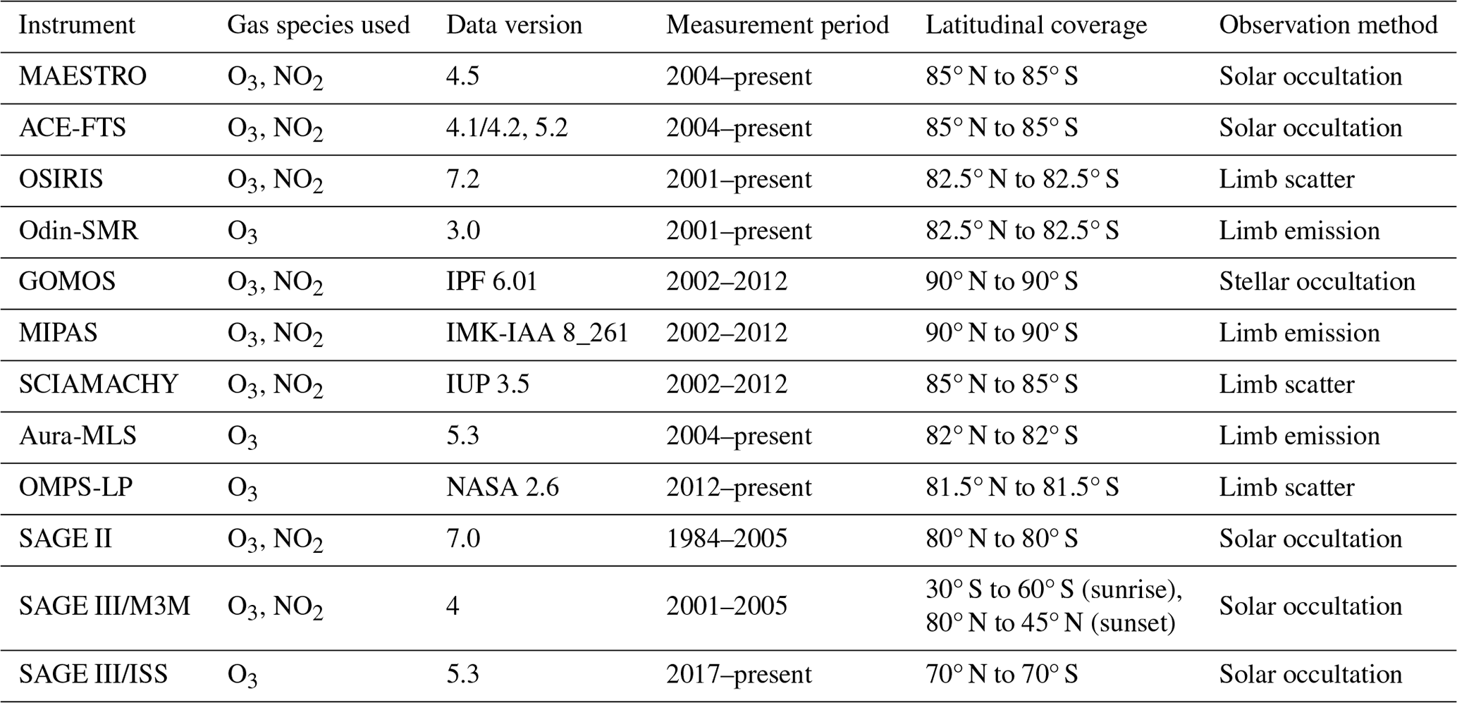
In this section, the MAESTRO instrument and the comparison ozone and NO₂ instruments used in this study are presented. The instruments are grouped by their measurement platforms, with the relevant information about the platform detailed in brief ahead of the corresponding instrument(s). Key details, including the data version, measurement technique, and the spatial and temporal coverage of these instruments, are presented in Table 1.

Table 1 Summary of the spatial and temporal coverage of the instruments used in this study, along with the trace gas species used here from each, the data version for the products employed, and the measurement technique of each instrument.

2.1 Atmospheric Chemistry Experiment

The ACE mission, aboard the Canadian SCISAT satellite, was launched into a circular low-Earth orbit (650 km altitude, 74° inclination) on 12 August 2003 (Bernath et al., 2005). As discussed above, there are two instruments aboard SCISAT: MAESTRO and ACE-FTS.

2.1.1 MAESTRO

The MAESTRO instrument aboard SCISAT is composed of a pair of grating spectrophotometers that record spectra between 285 and 1030 nm with a wavelength-dependent resolution of 1–2 nm (McElroy et al., 2007). The solar occultation measurements made by MAESTRO consist of (1) sequences of 60 spectra taken between the cloud tops and 100 km above the surface and (2) an additional 20 spectra taken between 100 and 150 km for use as reference spectra. The 1.2 km field of view (FOV) of MAESTRO on the limb, combined with typical measurement spacing of around 1 to 2 km, leads to an effective vertical resolution of 1–2 km for this instrument. Scientific operation of MAESTRO commenced in February 2004 and continues through to the present, despite the build-up of an unknown contaminant blocking the transmission of light with wavelengths shorter than 500 nm (Sioris et al., 2016; Bernath, 2017).

For the newest version of the MAESTRO products, version 4.5, measurements made by MAESTRO are used to retrieve volume mixing ratio (VMR) profiles of UV-ozone, NO₂, Vis-ozone, and optical depth. As with previous versions of the MAESTRO products, the general retrieval is based on a two-step approach wherein a modified differential optical absorption spectroscopy (DOAS) technique is used to obtain line-of-sight column densities at each measurement tangent height (McElroy et al., 2007; Kar et al., 2007; Bognar et al., 2019). However, unlike previous versions, a Twomey–Tikhonov inversion algorithm is used to invert these slant columns into VMR profiles. In the version 4.5 retrieval algorithm, the Vandaele et al. (2002) NO₂ and Serdyuchenko et al. (2011) ozone cross-sections are employed, and the retrieval includes a temperature correction based on the temperature-dependence of the ozone cross-sections. The new version 4.5 retrieval also incorporates improved Rayleigh scattering modelling and an improved algorithm for high-Sun reference spectrum calculation. The retrieval is performed on an altitude grid spanning from 5 to 80 km; however, the profile is provided on a grid spanning 0 to 100 km, extrapolating from the retrieved profile to the rest of the grid. Above 50 km, the data should be used with caution, as the retrieval is less constrained. As with previous versions of the MAESTRO retrieval, the version 4.5 inversion uses the ACE-FTS pressure and temperature profile data; however, this has been updated to use the ACE-FTS version 5.2 data, which address the possibility of a drift in the MAESTRO products produced using the ACE-FTS version 3.5/3.6 data that results from systematic CO₂ modelling errors discussed in Sheese et al. (2022). The version 4.5 dataset used covers the period from February 2004 to December 2023.

Before release, extreme outliers are removed from the MAESTRO dataset by filtering out profiles of ozone in which the maximum VMR between 5 and 50 km is greater than 30 ppmv or less than 0.01 ppmv and filtering out NO₂ profiles whose maximum VMR is greater than 20 ppbv or less than 0.01 ppbv over this same vertical range. In this study, in order to further screen the released MAESTRO version 4.5 data for any remaining outliers, four steps are taken. First, the UV products are only used up to their recommended end dates, specifically the end of June 2009 for NO₂ or the end of December 2009 for UV-ozone. Second, the most extreme outliers, which usually occur near the top of the MAESTRO profile where the retrieval is less constrained, are removed by filtering out values in excess of 500 ppmv for ozone or 500 ppbv for NO₂. Third, incomplete profiles, spanning less than 40 km in the vertical, are removed, as they have been found to be poorly constrained by the MAESTRO retrieval algorithm. Fourth, the remaining data are screened with a 10 median absolute deviations (MADs) filter, wherein all VMR values more than 10 MADs away from the median at each altitude are removed from the analysis. Excluding the date-based filters, this method of filtering removed <0.1 % of the MAESTRO Vis-ozone profiles, <0.1 % of the MAESTRO UV-ozone profiles, and <0.1 % of the MAESTRO NO₂ profiles.

2.1.2 ACE-FTS

The other instrument aboard SCISAT, ACE-FTS, is a Fourier transform spectrometer measuring the spectral range between 750 and 4400 cm⁻¹ with 0.02 cm⁻¹ spectral resolution (Bernath et al., 2005). ACE-FTS records solar absorption spectra at tangent heights spanning from the cloud tops to 150 km, with vertical spacing between 1.5 and 6 km and a vertical FOV of 3 to 4 km on the limb. As with MAESTRO, scientific operations of ACE-FTS commenced in February 2004 and continue through to the present.

The measurements made by ACE-FTS are used to retrieve vertical profile information about temperature, pressure, and VMR for several dozen trace gas species. The full retrieval process is described in Boone et al. (2005, 2013, 2020, 2023). However, in brief, this process involves establishing pressure and temperature profiles using the operational global weather assimilation and forecasting system managed by the Meteorological Service of Canada (Buehner et al., 2015) below approximately 18 km and through analysis of CO₂ spectral lines above this altitude; a global Levenberg–Marquardt nonlinear least-squares fitting algorithm is then subsequently used to determine VMR profiles with 3–4 km vertical resolution. In this work, two versions of the ACE-FTS profiles of ozone and NO₂ are used: the version 4.1/4.2 profiles, which have undergone prior validation efforts, and the new version 5.2 profiles, which expand the list of retrieved products from ACE-FTS measurements, contribute the pressure and temperature information used in the MAESTRO retrievals, and are considered the current working product (Boone et al., 2023). The ACE-FTS data used in this study cover the period from February 2004 to December 2023.

Quality flags have been developed for the ACE-FTS version 4.1/4.2 and version 5.2 products and have been applied to the ACE-FTS datasets used in this work (Sheese et al., 2015). As recommended, all measurements marked with quality flags >0 are removed in order to filter out extreme outliers.

The ACE-FTS version 4.1/4.2 profiles of NO₂ have been compared against coincident measurements from OSIRIS by Dubé et al. (2022) and against SAGE III/ISS by Strode et al. (2022). The former found that ACE-FTS NO₂ is smaller than that from OSIRIS by approximately 20 % at 18 km, larger than OSIRIS by about 10 % between 25 and 30 km, and again smaller than OSIRIS by approximately 20 % at 38 km, while the latter found ACE-FTS NO₂ to be less than that of SAGE III/ISS by between 10 % and 20 % over the stratosphere, with better agreement at lower altitudes. Strode et al. (2022) also compared ACE-FTS ozone against that from SAGE III/ISS and found ACE-FTS ozone to be about 5 % larger than that of SAGE III/ISS at 15 km, although within approximately 0 %–2 % up to about 45 km. Sheese et al. (2022) compared the version 4.1/4.2 ozone to measurements from MAESTRO, OSIRIS, Aura-MLS, SABER, and Odin-SMR and found that the weighted average difference showed that ACE-FTS ozone was larger than these other datasets by between 2 % and 9 % over the stratosphere, with the largest differences occurring around 30 km.

2.2 Odin

The Odin satellite was launched into a near-circular Sun-synchronous low-Earth orbit (600 km, 98° inclination) in February 2001 (Murtagh et al., 2002). The ascending (descending) node of Odin has drifted over time, from 18:00 LT (06:00 LT) (where LT denotes local time) to an hour later and then back to only half an hour later, due to a slight procession in its orbit (Llewellyn et al., 2004; Bourassa et al., 2014). Odin was designed for a mixed aeronomy/astronomy mission, splitting time between observation modes designed for each focus; however, since May 2007, Odin has solely made atmospheric observations. There are two main instruments aboard Odin: the Sub-Millimetre Radiometer (Odin-SMR) and the Optical Spectrograph and InfraRed Imaging System (OSIRIS).

2.2.1 Odin-SMR

The Odin-SMR instrument employs four tunable sub-millimetre radiometers that measure thermal limb emission in the 486–581 GHz spectral region and a millimetre radiometer that measures thermal emission around 119 GHz (Murtagh et al., 2002; Urban et al., 2005). Two autocorrelator spectrometers generate spectra from the observed signal with an 800 MHz bandwidth and a 2 MHz resolution; however, only two channels can be measured simultaneously. Under its typical stratospheric observation mode, Odin-SMR measures in two frequency bands centred at 501.8 and 544.6 GHz, respectively. During measurements, Odin-SMR scans from 7 km to between 70 and 110 km, depending on its observation mode, with a FOV of approximately 2 km on the limb, 1.5 km vertical measurement spacing below 50 km, and 6 km spacing above 50 km (Murtagh et al., 2002, 2020). Stratospheric observations are made every 2 d (every 3 d prior to May 2007), and approximately 900 profiles are recorded per day. Scientific operations of Odin-SMR began in July 2001 and continue through to the present.

The measurements from Odin-SMR are used to retrieve VMR profiles of several trace gas species as well as temperature. Eriksson (2020) details the retrieval, which involves using the optimal estimation method with a Levenberg–Marquardt iteration scheme to retrieve profiles on measurement-tangent-point pressure levels. Estimates of geometrical altitude are provided alongside the retrieved products. The products retrieved vary with the Odin-SMR observation mode, and multiple ozone products are currently produced from three separate channels. In this study, the version 3.0 ozone product from the 544.6 GHz channel is used, as recommended by Murtagh et al. (2020) and Pérot et al. (2020). While this ozone product spans from 11 to 109 km, the valid range is from 17 to 77 km. The vertical resolution of these profiles is 2–3 km over the valid range. The version 3.0 Odin-SMR data used in this study cover the period from February 2004 to September 2022.

These data are screened for quality control before being released. The two filters applied require that the minimum value for the Levenberg–Marquardt damping parameter is below 2 and that the spectral fit residuals are less than 1.5 K (Pérot et al., 2020). No further filtering is applied in this study to the Odin-SMR products.

The version 3.0 ozone retrieved from the 544.6 GHz channel has been previously compared to other coincident measurements in Murtagh et al. (2020) and Sheese et al. (2022). In the former, Odin-SMR ozone was compared against that of OSIRIS, MIPAS, and Aura-MLS. They found that Odin-SMR ozone was, on average, about 10 %–15 % smaller than MIPAS and OSIRIS between 20 and 50 km and about 5 %–10 % smaller than MLS over this same range. Comparisons against ACE-FTS by Sheese et al. (2022) showed that Odin-SMR ozone is biased low by about 5 %–10 %.

2.2.2 OSIRIS

OSIRIS consists of a grating optical spectrograph (OS) and an infrared imager (IRI). The former records Rayleigh- and Mie-scattered sunlight spectra between 280 and 810 nm with 1–2 nm resolution, while the latter measures airglow (Llewellyn et al., 2004). OSIRIS records limb radiance at tangent heights between 7 and 70 km under its typical (stratospheric) operation mode, with altitude-dependent vertical spacing of 1 to 2 km and a vertical FOV on the limb of about 1 km (Haley et al., 2004). Between 30 and 60 profiles are recorded every orbit, with 15 orbits completed per day. Due to the orbital geometry of Odin, coverage focuses on the Southern Hemisphere between October and February and the Northern Hemisphere between March and September. Routine operation of OSIRIS began in November 2001 and continues through to the present.

Limb-radiance profiles recorded by OSIRIS are used to retrieve profiles of ozone, NO₂, and sulfate aerosol from the cloud tops to 60 km (Degenstein et al., 2009). Details of the version 7.2 NO₂ and ozone retrievals used in this study can be found in Dubé et al. (2022) and Bognar et al. (2022), respectively. Broadly, these retrievals employ a Levenberg–Marquardt algorithm to retrieve number density profiles of these two species using pressure and temperature data from the Modern-Era Retrospective analysis for Research and Applications Version 2 (MERRA-2; Gelaro et al., 2017). These products have a vertical resolution of 1.5 km for ozone and 2–3 km for NO₂, In this study, the reported number density values are converted into VMRs using the MERRA-2 temperature and pressure information employed in the retrievals. The OSIRIS data used in this study cover the period from February 2004 to December 2023.

The OSIRIS data are screened for quality control ahead of release. This involves screening the limb-radiance measurements for clouds or cosmic rays (Bognar et al., 2022). The NO₂ product is further filtered through the application of an averaging-kernel-based criterion for determining the functional lower bound of the retrieved product (Dubé et al., 2022). No further data filtering was applied in this study.

Dubé et al. (2022) compared version 7.2 OSIRIS NO₂ with that from ACE-FTS and SAGE III/ISS. They found that OSIRIS NO₂ was larger than that of ACE-FTS around the tropopause in the Northern Hemisphere, with differences as large as 50 %, as well as above 35 km, with differences of 10 %–20 %, whereas ACE-FTS had larger NO₂ values elsewhere, by about 10 %. Compared with SAGE III/ISS the OSIRIS product was found to be smaller over virtually all of the upper troposphere and stratosphere, albeit with better agreement found at higher altitudes. The average difference in these comparisons throughout the stratosphere is about 20 %. Similar results were found by Strode et al. (2022) for NO₂. Strode et al. (2022) also found version 7.2 OSIRIS ozone to be within about 5 % of SAGE III/ISS over much of the stratosphere, with larger differences, of 10 %–15 %, found below 20 km.

2.3 Envisat

The ENVIronmental SATellite (Envisat) was launched into a Sun-synchronous low-Earth orbit (800 km, 98.55° inclination) in February 2002 (Bertaux et al., 2010). Envisat had an ascending (descending) node at 22:00 LT (10:00 LT) and operated until April 2012, when contact was lost with the satellite. Aboard Envisat were the Global Ozone Monitoring by Occultation of Stars (GOMOS), the Michelson Interferometer for Passive Atmospheric Sounding (MIPAS), and the Scanning Imaging Absorption spectroMeter for Atmospheric CHartographY (SCIAMACHY) instruments.

2.3.1 GOMOS

The GOMOS instrument was composed of a pair of grating spectrometers, operating in the UV–visible (between 248 and 690 nm) with 0.8 nm resolution and in the infrared (IR) (between 750–776 nm and 916–956 nm) with 0.13 nm resolution, along with a pair of photometers (Kyrölä et al., 2004; Bertaux et al., 2010). GOMOS measured atmospheric transmission spectra using a stellar occultation technique, employing about 180 stars as light sources and making measurements from between 5 and 20 km, depending on the presence of clouds and the brightness of the reference star, to 150 km (Tamminen et al., 2010). Measurements were spaced by 0.5–1.6 km and were recorded during both night (dark limb) and day (bright limb) as viewed by the instrument. About 600 occultations were recorded per day, with 100–200 of those being dark-limb measurements. Scientific operation of GOMOS began in March 2002 and ended in April 2012.

GOMOS stellar occultation measurements are used to retrieve vertical profiles of five trace gases as well as aerosols. As detailed in Kyrölä et al. (2010), the UV–visible retrievals, which produce the ozone and NO₂ products, use a maximum-likelihood method to obtain tangent column densities that are then inverted using Tikhonov regularization to determine number density profiles, with the inversion set up to produce profiles at a desired vertical resolution. For ozone the vertical resolution is 2 km below 30 km, increasing to 3 km at and above 40 km, whereas the vertical resolution is 4 km for the other products (Kyrölä et al., 2010; Tamminen et al., 2010). The air density estimates required for this come from the European Centre for Medium-Range Weather Forecasts (ECMWF) 24 h forecast below 1 hPa and from the MSIS-90 model (Hedin, 1991) above 1 hPa. The Instrument Processing Facility (IPF) version 6.01 GOMOS retrieval products, which are made available on a uniform 1 km vertical grid, are used in this study, and the number density profiles are converted into VMR profiles using the air density profiles used for the retrieval. The GOMOS data used in this study cover the period from February 2004 to April 2012.

The GOMOS product quality is impacted by the brightness of the target star used for occultations. Following product usage recommendations, only those ozone measurements made using stars that reliably produce viable results have been used in this work (Kyrölä et al., 2017). The ozone product is also provided with quality flags that identify the presence of outliers in the stratosphere, and all profiles flagged with a stratospheric outlier have been filtered from analysis. Additionally, it has been found that the bright-limb occultations are strongly affected by scattered solar light; thus, only the dark-limb measurements are used in this study. Beyond this, measurement-specific altitude validity ranges are provided for each gas, and only data within this range are included in this study (Kyrölä et al., 2017). Finally, a 10-MAD filter is applied to the GOMOS data, removing all VMR values more than 10 MADs away from the median at each altitude.

GOMOS IPF version 6 ozone and NO₂ profiles have previously been compared in Adams et al. (2014) and Sheese et al. (2016), respectively. The former found that the GOMOS ozone product is within approximately 2.5 % of that from OSIRIS between 20 and 50 km, but the GOMOS product is over 20 % larger than that of OSIRIS below 20 km. Sheese et al. (2016) found that ACE-FTS agreed with GOMOS NO₂ to within 20 % between about 23 and 40 km, with ACE-FTS showing less NO₂ at lower altitudes and more NO₂ above approximately 27 km. Climatological comparisons by Hegglin et al. (2021) found that IPF version 6.01 GOMOS ozone is lower than that from a multi-instrument mean (MIM) by more than 20 % near the tropopause and by between 0 % and 10 % over most of the stratosphere.

2.3.2 MIPAS

MIPAS was a Fourier transform spectrometer aboard Envisat that measured limb emission spectra over five mid-IR bands between 685 and 2410 cm⁻¹ (Fischer et al., 2008). Between July 2002 and March 2004, MIPAS was operated at its full spectral resolution, 0.035 cm⁻¹; however, instrument subsystem issues led to a gap in measurements between April and December 2004, after which time it was operated at a reduced resolution of 0.0625 cm⁻¹ (Kiefer et al., 2023). MIPAS had a 3 km vertical FOV and, during the full-resolution period, made measurements between 6 and 68 km with 3 to 6 km spacing, producing about 1000 observations per day. When operated at reduced resolution, nominal operations involved MIPAS measuring between 6 and 70 km with 1.5 to 4 km spacing, making approximately 20 % more measurements per day than during full-resolution operation (Fischer et al., 2008; von Clarmann et al., 2009). Scientific operation of MIPAS ended in April 2012.

Limb emission spectra recorded by MIPAS are used to retrieve profiles of temperature and over two dozen trace gases. Different MIPAS retrievals are performed at multiple institutions, and this study employs that produced by the Institut für Meteorologie und Klimaforschung (IMK) in collaboration with the Instituto de Astrofísica de Andalucía (IAA). Compared with the MIPAS retrievals from other institutions, Laeng et al. (2017) found the ozone product from the IMK-IAA retrieval to be less biased by a factor of 2. The IMK-IAA retrieval is described in Funke et al. (2001), von Clarmann et al. (2003, 2009), and Kiefer et al. (2021). It is based on multiparameter fitting of spectra using Tikhonov regularization. Briefly, temperature profiles are retrieved and the tangent height pressures are determined using the hydrostatic equation. Trace gas species are then retrieved using these profiles, first for species with major contributions to the IR spectra, including ozone and NO₂, and then for all remaining species. In this study, the version 8 IMK-IAA products from the reduced-resolution period measured in the nominal operation mode (version 8_261) are used, with no data used from the full-resolution MIPAS period, as only 6 weeks of overlap are found with MAESTRO. This ozone product has a vertical resolution of about 3–4 km, while the NO₂ product has a vertical resolution of 3–6 km, increasing with altitude in the stratosphere. The MIPAS data used in this study cover the period from November 2004 to April 2012.

Adapting the work of Funke et al. (2023), the MIPAS IMK-IAA data used in this study are screened for quality through analysis of the reduced χ² of the retrieval fit, by filtering out any profile whose reduced χ² is equal to or larger than 5. Following this, data were only used if the visibility marker included with the data was set to 1 for a given tangent altitude, indicative of a cloud-free observation at that altitude.

Prior versions of the MIPAS IMK-IAA ozone and NO₂ products have been validated against sets of coincident measurements from other instruments. Sheese et al. (2017) found that version 5 MIPAS ozone agrees with ACE-FTS to within 5 % between 10 and 45 km, above which MIPAS was found to yield less ozone by about 10 %–20 % up to about 60 km. They also found agreement for MIPAS ozone to within about 5 % of Aura-MLS, up to about 60 km. Recent climatology studies of the version 5 MIPAS ozone found that, in comparisons against a MIM, MIPAS was within 5 % over much of the stratosphere, only showing significantly poorer agreement around the tropopause (Hegglin et al., 2021). Comparisons of the version 5 NO₂ from MIPAS against ACE-FTS showed that the former yielded less NO₂ below 30 km, by about 30 %, above which it yielded increasingly more NO₂ with altitude, reaching differences in excess of 60 % (Sheese et al., 2016). Better agreement, to within about 10 %, was found between MIPAS NO₂ and both OSIRIS and SCIAMACHY below 30 km (Sheese et al., 2016).

2.3.3 SCIAMACHY

SCIAMACHY was a passive imaging grating spectrometer that measured within the spectral range between 240 and 2380 nm over eight channels, with a channel-dependent spectral resolution between 0.24 and 1.48 nm (Burrows et al., 1995; Bovensmann et al., 1999). Designed for mixed operation, SCIAMACHY made limb scatter, nadir backscatter, and solar/lunar occultation measurements; however, only the results from the limb scatter measurements are used here. These limb scatter measurements were recorded at tangent altitudes from just below the surface up to about 92 km, with 3.3 km vertical spacing and a vertical FOV of about 2.6 km on the limb. About 1000 limb scatter measurements were made per day. Scientific operation of SCIAMACHY commenced August 2002 and continued through to April 2012.

Number density profiles are retrieved from the SCIAMACHY limb measurements for several species, including ozone and NO₂. In this study, the version 3.5 scientific retrievals are used. These retrievals, described in detail in Jia et al. (2015) for ozone and in Bauer et al. (2012) for NO₂, employ a DOAS technique and Tikhonov regularization to retrieve profiles of ozone between 8 and 65 km and of NO₂ between 10 and 45 km. Both species are retrieved on the measurement tangent height grid, and the retrievals have a vertical resolution of 3–5 km. Pressure and temperature data for this retrieval come from the ECMWF reanalysis and are used here to convert the number density profiles into VMR profiles. The SCIAMACHY data used in this study cover the period from February 2004 to April 2012.

Following quality control measures from prior analysis of the SCIAMACHY measurement products (e.g., Gebhardt et al., 2014; SPARC-DI, 2017; Sofieva et al., 2021), data are filtered out if measured over the South Atlantic Ocean (20–70° S, 0–90° W) to remove the impact of the South Atlantic Anomaly. No further filtering is applied.

Profile comparisons of SCIAMACHY NO₂ against ACE-FTS by Sheese et al. (2016) showed that the SCIAMACHY version 3.1 product is biased low below about 30 km, with relative differences decreasing from 70 % at about 15 km to 20 % at 25 km, above which the two sets of profiles agree to within 20 %. However, cross-comparisons in the same study showed that the SCIAMACHY profiles agreed with OSIRIS and MIPAS profiles to within about 15 % over most of the stratosphere. For the SCIAMACHY version 3.0 ozone product, Jia et al. (2015) found a difference of less than 10 % when compared against ozonesonde measurements between 20 and 30 km, with SCIAMACHY showing less ozone than the ozonesondes. Climatology-based comparisons of version 3.5 SCIAMACHY ozone against a MIM showed that ozone concentrations from SCIAMACHY in the stratosphere are larger than the mean by 0 %–10 % below 25 km and smaller than the mean by approximately the same amount above this altitude (Hegglin et al., 2021)

2.4 Suomi-NPP

The Suomi National Polar-orbiting Partnership (Suomi-NPP) was launched into a Sun-synchronous low-Earth orbit (834 km, 98.8° inclination) in October 2011 (Rault and Loughman, 2013). With an ascending (descending) node at 13:30 LT (01:30 LT), Suomi-NPP is host to five instruments, including the Ozone Mapping and Profiler Suite (OMPS).

2.4.1 OMPS-LP

OMPS is composed of three sensors: a nadir total column mapper (NM), a nadir profiler (NP), and a limb profiler (LP). The nadir sensors, not used in this study, measure backscattered UV radiation, while the OMPS-LP measures limb-scattered radiation from 290 to 1000 nm with a wavelength-dependent spectral resolution ranging from 1.5 nm in the UV to 40 nm at 1000 nm (Flynn et al., 2004; Jaross et al., 2014). OMPS-LP is a prism spectrometer that measures spectra from three vertical slits offset horizontally by 4.25° (250 km across track). Each slit spans 112 km in the vertical, to ensure coverage from 0 to 80 km, with approximately 1 km sampling and a 1.3–1.7 km vertical FOV. Two spectra are recorded simultaneously from each slit with different integration times to account for differences in spectral intensity, and approximately 2400 observations are made per day from each slit. Scientific operation of the OMPS-LP began in February 2012 and continues through to the present.

OMPS-LP measurements are used to derive profiles of ozone and aerosol extinction. The ozone retrieval, detailed in Rault and Loughman (2013) and Kramarova et al. (2018), involves normalizing the measured radiances with measurements made at 60.5 km for the UV and 40.5 km for the visible, constructing wavelength pairs or triplets, and applying a Tikhonov regularization to obtain an estimate for ozone number density profiles. The retrieved profiles span from the cloud tops, or 12.5 km, to 57.5 km, with about a 1.8 km vertical resolution. Values are reported on a uniform 1 km grid along with the MERRA-2-derived temperature and pressure information used for the retrievals. These temperature and pressure fields are used to convert the number density profiles into VMR in this work. The version 2.6 ozone product is used in this study, which only employs measurements made by the central vertical slit of OMPS-LP due to stray light affecting the side-channel measurements (Kramarova and DeLand, 2023). This dataset covers the period from February 2012 to December 2023.

The OMPS-LP ozone data are provided with a set of retrieval metrics and quality screening flags. Following the recommendations for the version 2.6 product in Kramarova and DeLand (2023), data were filtered out if the retrieval algorithm convergence was greater than 10, and the ozone product was only used if the number of retrieval iterations was between 2 and 7. As for the quality flags, data were filtered out if the polar mesospheric cloud (PMC) flag indicated the presence of PMCs that affected the measurements, if the ozone quality flag indicated a wavelength shift in the algorithm, or if the quality measurement vector flag indicated a poor-quality profile.

The OMPS-LP version 2.5 ozone product has been validated by comparison with ACE-FTS, Aura-MLS, and OSIRIS by Kramarova et al. (2018). They found OMPS-LP ozone to be between 10 % and 15 % lower than that of ACE-FTS, Aura-MLS, and OSIRIS between 12.5 and about 20 km, above which differences were generally around 5 % up to 30 km. Between 30 and 40 km the OMPS-LP version 2.5 product was found to be 10 % larger than that of OSIRIS, and 5 % larger than that of ACE-FTS and Aura-MLS. Finally, above 40 km, OMPS-LP yielded progressively less ozone with altitude than the other instruments, reaching differences of approximately 10 %–20 % at 50 km. Further comparisons by Strode et al. (2022) showed the version 2.5 OMPS-LP ozone data to be generally larger than SAGE III/ISS below 20 km and above 40 km, whereas smaller values were observed in between these two altitudes, although good general agreement was found overall (to within 10 %).

2.5 Aura

The Aura satellite was launched into a Sun-synchronous low-Earth orbit (705 km, 98° inclination) in July 2004 (Waters et al., 2006). Aura has an ascending (descending) node at 13:45 LT (01:45 LT) and is host to four instruments, including the Aura Microwave Limb Sounder (Aura-MLS).

2.5.1 Aura-MLS

The Aura-MLS instrument is composed of seven radiometers that measure microwave thermal emission in five spectral regions corresponding to 118, 190 GHz, 240 GHz, 640 GHz, and 2.5 THz (Waters et al., 2006; Livesey et al., 2022). During operations, Aura-MLS scans the radiometer antennae through the limb of the atmosphere, from the surface to about 90 km, every 25 s, resulting in about 3500 observations per day. The vertical FOV on the limb of the radiometers varies from 1.5 to 6.5 km, and measurements are made with approximately 1 km vertical spacing. Scientific operations of Aura-MLS began in August 2004 and continue through to the present.

Measurements made by Aura-MLS are used to retrieve vertical profiles of temperature, geopotential height, and VMR of 15 trace gas species, including ozone. This process, detailed in Waters et al. (2006) and Livesey et al. (2022), begins with establishing estimates of temperature and tangent pressure through analysis of O₂ and O₂ isotopologues, followed by establishing estimates of nine trace gas species, including ozone. Over multiple phases, these estimates are refined, and the remaining meteorology and trace gas fields are subsequently determined. The retrievals use an optimal estimation approach, and the products are retrieved on fixed pressure surfaces, with six pressure levels per decade. The vertical resolution of the retrievals varies from 2.5 km in the lower stratosphere to 5 km in the upper stratosphere. In this study, version 5.3 of the Aura-MLS ozone product is used, which requires transformation from its native pressure vertical coordinate to an altitude coordinate. This is accomplished by interpolating Aura-MLS ozone profiles that are coincident with MAESTRO profiles (see Sect. 3 for coincidence criteria) onto the MAESTRO altitude grid using the ACE-FTS pressure (which is used as the pressure for the MAESTRO retrievals), at each altitude for the interpolation. The Aura-MLS data used in this study cover the period from August 2004 to December 2023.

The version 5.3 Aura-MLS data files include several quality- and retrieval-related fields necessary for screening the retrieved data. Following the recommendations of Livesey et al. (2022), the Aura-MLS ozone data used in this study have been filtered to remove any profiles with quality flags less than 1.0 (showing poor radiance fits), with convergence values greater than 1.03 (showing divergence from the expected radiance fit), and with negative precision estimates (indicating a non-physical effect arising from the a priori data). Additionally, only profiles with even status fields were included, which exclude data with questionable profiles or those affected by the presence of clouds. Lastly, ozone data are only used from the pressure levels between 261 and 0.001 hPa, which is the valid range for these ozone retrievals.

The Aura-MLS version 5.1 ozone profiles have been compared to coincident profiles from ACE-FTS in Sheese et al. (2022), who found that Aura-MLS ozone was approximately 5 %–10 % smaller than that of ACE-FTS over the stratosphere. Wang et al. (2020) found that Aura-MLS version 4.1 ozone is 0 %–5 % smaller than that of SAGE III/ISS over most of the stratosphere, showing more ozone only above 45 km. Climatological studies of Aura-MLS version 4.2 ozone against a MIM show a slight negative bias of 0 %–5 % over most of the stratosphere (Hegglin et al., 2021)

2.6 ERBS

The Earth Radiation Budget Satellite (ERBS) was launched into a circular low-Earth orbit (610 km, 57° inclination) in October 1984 (Mauldin III et al., 1985; McCormick, 1987). Despite several hardware failures, ERBS remained operational until it was decommissioned in August 2005 (Damadeo et al., 2013). Aboard ERBS was the Stratospheric Aerosol and Gas Experiment II (SAGE II) instrument.

2.6.1 SAGE II

SAGE II was a seven-channel grating spectrometer that measured between 385 and 1020 nm (Mauldin III et al., 1985; McCormick, 1987). Measuring from the cloud tops to about 150 km, SAGE II recorded solar occultation measurements during sunrise and sunset with a 0.5 km vertical FOV on the limb. Rather than remaining fixed on the Sun's centre, this FOV was scanned vertically across the Sun disk, allowing for multiple measurements to be made at approximately the same altitude (McCormick et al., 1989; Damadeo et al., 2013). This resulted in an approximate 1 km vertical resolution. Scientific operations of SAGE II began in October 1984, and 15 sunrise and 15 sunset measurements were made per day until July 2000 (Wang et al., 2002). After this time, a pointing problem led to a reduction in the number of daily measurements to about 16 in total per day. Scientific operations ceased in August 2005, when ERBS was decommissioned.

Measurements from SAGE II are inverted to yield profiles of ozone, aerosol, NO₂, and water vapour using the algorithm detailed in Chu et al. (1989) and Damadeo et al. (2013). Slant-path transmission profiles are calculated from the solar occultation measurements and are used to derive species-specific slant-path column densities using a least-squares fit. These are inverted to generate vertical profiles using an onion-peeling algorithm. This process requires temperature and pressure data, which come from the Modern-Era Retrospective analysis for Research and Applications (MERRA; Rienecker et al., 2011) up to 0.1 mbar, above which the lapse rate from the Global Reference Atmospheric Model-1995 (GRAM-95; Justus and Johnson, 1997) is used. In this study, the version 7.0 SAGE II products are used. These products span from the cloud top to 70 km for ozone and up to 50 km for NO₂, and they are provided on a uniform 0.5 km grid. Air density data used in the retrieval are employed to convert the number density profiles into VMR. The SAGE II data used in this study cover the period from August 2004 to August 2005.

The SAGE II ozone data were screened for outliers using the retrieval uncertainty estimates and the aerosol extinction values, following the recommendations of Wang et al. (2002) and Kremser et al. (2020). Screening with the former led to the exclusion of all ozone data points with an uncertainty estimate of over 300 %, all points below 35 km with an uncertainty estimate over 200 %, and all profiles with an uncertainty estimate of more than 10 % in the 30–50 km range. For the latter, data points were excluded (1) below the altitude at which an aerosol extinction value exceeded 0.006 km⁻¹ and (2) below the altitude at which the 525 nm aerosol extinction value exceeded 0.001 km⁻¹ if the ratio of the 525–1020 nm aerosol product fell below 1.4. In addition, the version 7.0 SAGE II product is provided with a cloud filter field, which denotes altitudes affected by the presence of clouds, and all data for both ozone and NO₂ affected as such were removed.

The SAGE II version 7.0 ozone product has been previously validated by Hubert et al. (2016), who found that SAGE II ozone was generally within 4 % of coincident ozonesonde measurements between 20 and 40 km but that SAGE II underestimated ozone by 10 %–15 % below 20 km. Adams et al. (2013) found similar results when comparing coincident SAGE II version 7.0 profiles with those from OSIRIS, with the two ozone datasets agreeing to within 5 % above about 15 km, below which differences increased to 10 %, with SAGE II version 7.0 generally yielding less ozone than OSIRIS. Climatological comparisons of SAGE II ozone against a MIM by Hegglin et al. (2021) suggest that SAGE II underestimates ozone across the entire stratosphere; however, this difference is usually less than 5 %, increasing to 10 %–20 % around the tropopause. Finally, climatologies of SAGE II version 6.2 NO₂ have also been compared to a MIM, and differences are within 20 % over most of the stratosphere, with a low bias in the middle stratosphere and high bias above and below this region (SPARC-DI, 2017).

2.7 Meteor-3M

The Meteor-3M satellite was launched into a Sun-synchronous low-Earth orbit (1020 km, 99.5° inclination) in December 2001 (Mauldin III et al., 1998; Thomason et al., 2010). The ascending (descending) node of the Meteor-3M was at 09:00 LT (21:00 LT), and several instruments were aboard the platform, including the Stratospheric Aerosol and Gas Experiment III/Meteor-3M (SAGE III/M3M). Meteor-3M operations ceased in March 2006 (Thomason et al., 2010).

2.7.1 SAGE III/M3M

The SAGE III/M3M instrument was composed of a grating spectrometer, which measured the spectral region from 280 to 1040 nm over 86 spectral channels, and a single photodiode that measured near 1550 nm (Mauldin III et al., 1998; Thomason et al., 2010). SAGE III/M3M made solar and lunar occultation measurements, although only the former are considered for this study due to the limited number of lunar observations available. Approximately 15 sunrise and 15 sunset measurements were made per day in solar occultation mode; however, due to the orbital characteristics of the Meteor-3M, these measurements were made only at high northern latitudes (45–80° N) for sunset measurements and at middle southern latitudes (25–60° S) for sunrise measurements. During solar occultation measurements, the FOV of SAGE III/M3M, approximately 0.5 km on the limb, was repeatedly scanned across the solar disk, covering altitudes from the cloud tops to approximately 300 km. This resulted in an effective vertical resolution of 1 km. Scientific operations of SAGE III/M3M began in February 2003 and continued through to March 2006.

SAGE III/M3M solar occultation measurements are used to retrieve number density profiles of several gases as well as profiles of aerosol extinction, temperature, and pressure. The SAGE III/M3M ozone and NO₂ retrieval algorithm is detailed in the SAGE III Algorithm Theoretical Basis Document (SAGE III ATBD, 2002) and Wang et al. (2006). This algorithm uses a multiple-linear-regression technique to determine slant-path column densities of ozone and NO₂ simultaneously from derived slant-path optical depth measurements. These columns are then inverted using a Chahine technique to give vertical profiles on a uniform 0.5 km grid. NO₂ is retrieved from the cloud tops to 50 km, while ozone is retrieved up to 85 km. The retrieval requires temperature and pressure information for the atmosphere, which comes from the National Oceanic and Atmospheric Administration (NOAA) National Centers for Environmental Prediction (NCEP) below 0.4 hPa, above which climatological data from GRAM-95 are used (Justus and Johnson, 1997). This information is used to convert the SAGE III/M3M number density profiles into VMR profiles. The version 4 SAGE III/M3M data products are used in this study for the period from February 2004 to December 2005.

The SAGE III/M3M data are pre-screened by the retrieval team before release, although Thomason et al. (2010) recommends additional filtering for several periods in early 2002 during which poor ephemeris data affected pointing knowledge. However, as only SAGE III/M3M data coincident with MAESTRO data are used here, no additional filtering was necessary.

SAGE III/M3M version 4 ozone data were compared against coincident ozonesonde measurement by Davis et al. (2016), and agreement to within 5 % over the entire stratosphere was found. Climatological comparisons of the version 4 SAGE III/M3M ozone against a MIM climatology show agreement to within 10 % over virtually the entire stratosphere, with SAGE III/M3M yielding more ozone in the middle stratosphere and less in the upper and lower stratosphere (SPARC-DI, 2017). Comparisons of NO₂ zonal mean profiles against MIM profiles in SPARC-DI (2017) showed that version 4 SAGE III/M3M NO₂ is about 10 % higher than the MIM in the middle stratosphere, while differences below 20 km can exceed 30 % and those above 35 km can exceed 50 %. This is in agreement with the work of Sheese et al. (2016), who compared version 3 SAGE III/M3M NO₂ against that of ACE-FTS and found the SAGE III/M3M product to be about 10 % larger than that of ACE-FTS between approximately 22 and 40 km.

2.8 International Space Station

The International Space Station (ISS) has been in low-Earth orbit (420 km, 51.6° inclination) since November 1998. Aboard the ISS is an instrument array that has cycled over time, including the Stratospheric Aerosol and Gas Experiment III on the International Space Station (SAGE III/ISS), which was installed in February 2017.

2.8.1 SAGE III/ISS

SAGE III/ISS is a grating spectrometer that operates from 280 to 1035 nm over 86 spectral channels, with an additional photodiode that measures at 1542 nm (McCormick et al., 2020; Wang et al., 2020). SAGE III/ISS makes solar and lunar occultation measurements, although only the former are considered here, with approximately 15 sunrises and 15 sunsets measured each day. Solar occultation measurements are made by scanning the approximately 0.5 km effective FOV of the instrument across the solar disk, resulting in multiple measurements at each altitude. Scientific operations of SAGE III/ISS commenced in June 2017 and continue through to the present (Dubé et al., 2021).

The solar occultation measurements from SAGE III/ISS are used to produce vertical profiles of ozone, water vapour, NO₂, aerosol extinction, temperature, and pressure. The ozone and NO₂ algorithms, detailed in the SAGE III ATBD (2002) and Wang et al. (2020), consist of determining slant-path optical depth profiles and then using a multiple-linear-regression technique to determine slant-path number density profiles. This retrieved NO₂ is used to derive a second ozone product, termed the aerosol ozone (AO3) product, using a least-squares technique akin to the SAGE II retrieval. The slant-path number density profiles are converted to vertical number density profiles using a global fit inversion method. The resulting profiles are produced on a uniform 0.5 km grid, spanning from 0 to 70 km with about a 1 km vertical resolution. Temperature and pressure data for the inversion come from MERRA-2, and the air density calculated from these fields is used in this study to convert the profiles from number density to VMR. In this work, the version 5.3 SAGE III/ISS products are used, with the AO3 product being used for ozone, which Wang et al. (2020) showed to have the smallest biases and best precision of the SAGE III/ISS ozone products, as determined from comparisons with an ensemble of satellite, ozonesonde, and lidar measurements. The SAGE III/ISS data used in this study cover the period from July 2017 to December 2023.

Prior to release, the SAGE III/ISS products are assessed by the mission team to determine their overall quality and remove any failed retrievals (SAGE III/ISS Data Products User’s Guide, 2023). Quality flags are included with the data for each retrieved profile, denoting measurements with negative or fill data in their slant-path profile; however, as these flagged properties do not preclude the inversion from generating a viable number density profile, these flags have not been used to filter the data. No further filtering has been applied to the dataset.

The SAGE III/ISS version 5.1 ozone was compared against coincident measurements from ACE-FTS in McCormick et al. (2020), with agreement being found to within about 5 % between 20 and 50 km and with seasonal variation with respect to which product yielded more ozone. Similarly, Wang et al. (2020) found that Aura-MLS agreed with version 5.1 SAGE III/ISS ozone to within 5 % between 18 and 50 km, with SAGE III/ISS yielding slightly more ozone overall. Comparisons against OSIRIS showed OSIRIS ozone to be about 5 % smaller over the stratosphere, while comparisons with OMPS-LP showed that OMPS-LP yielded more ozone, by about 5 %–10 %, around 30 km, above and below which the differences increase to 20 %, with SAGE III/ISS yielding more ozone (Wang et al., 2020). Comparisons by Dubé et al. (2022) showed that SAGE III/ISS version 5.2 NO₂ had larger values over most of the stratosphere, by about 20 %, compared with OSIRIS. Further comparisons of SAGE III/ISS version 5.2 NO₂ against that of ACE-FTS, performed by Strode et al. (2022), showed that SAGE III/ISS agrees to within about 25 % with ACE-FTS over the stratosphere, albeit with a consistent high bias. They also found that OSIRIS NO₂ was about 50 %–70 % smaller than that of SAGE III/ISS below 20 km, but this difference decreased with altitude to about 10 %–20 % near 40 km.

3 Comparison methodology

All of the satellite measurement datasets used were interpolated onto a uniform 1 km vertical grid, spanning from 0 to 100 km, chosen to match the effective vertical resolution of the MAESTRO dataset. The datasets were linearly interpolated without the use of smoothing using instrument averaging kernels (e.g., Dupuy et al., 2009; Adams et al., 2012). As the MAESTRO version 4.5 retrievals are only weakly constrained above 80 km, this study focuses between 5 and 80 km, where most of the retrieved profile information is located.

In order to compare measurements from different instrument sets, spatial and temporal coincidence criteria were employed. Following analyses by Sheese et al. (2021), who compared the effects of coincidence criteria against geophysical variability, measurements in this study are deemed coincident if they are made within 8 h of each other and within 1000 km. If multiple measurements from a comparison dataset are coincident with a MAESTRO profile, only the profile measurement closest in time is used for analysis; thus, every MAESTRO profile is coincident with at most one profile from each other satellite dataset.

As a solar occultation instrument, MAESTRO has relatively sparse spatial and temporal sampling; therefore, when employing coincidence criteria for comparisons, as done here, the potential exists for sampling biases to impact the results. This is likely to occur when comparison instruments also provide sparse or seasonally varying coverage, with the biases resulting from comparisons that do not wholly capture the state of the atmosphere or that result in systematic differences in sampling locations. In this study, a number of instruments with both sparse and dense sampling are employed. The latter instruments, which include Odin-SMR, SCIAMACHY, MIPAS, Aura-MLS, and OMPS-LP, yield comparisons with minimal potential for sampling biases to impact the results of the analysis, as the measurement comparisons are generally evenly distributed across space and time. Although ACE-FTS is a solar occultation instrument with the sparse sampling which that entails, it shares a line of sight with MAESTRO; hence, every measurement made by MAESTRO is coincident with one from ACE-FTS, thereby avoiding any systematic differences in measurement locations.

In contrast, OSIRIS is a densely sampling instrument that possesses a seasonal asymmetry in its coverage, generally only covering one hemisphere at a time, while the remaining four instruments employed in this study, GOMOS and the three SAGE instruments, all provide sparse sampling. The sparse sampling of these last four instruments is due to the limitations, addressed above, of the solar occultation technique employed by the SAGE instruments and the limited number of viable stellar occultation measurements made by GOMOS. Thus, for OSIRIS, GOMOS, and the SAGE instruments, there exists the possibility that any comparisons made with them will be affected by sampling biases. This is particularly true for SAGE II, as it was only operating at a 50 % duty cycle throughout the SAGE II–MAESTRO overlap period, which, when combined with the orbits of ERBS and SCISAT, causes all coincident measurements to be largely confined to a few narrow groupings, often near the edges of the polar vortex where variability is high.

Despite the potential for sampling biases, this study includes these sparse sampling/seasonally asymmetric datasets for the assessment of the MAESTRO version 4.5 products to allow for an overview of the MAESTRO data in comparison to a diverse suite of measurements made using multiple techniques, with the caveat that some of these comparisons might be affected by sampling biases and should be considered as part of an ensemble of comparisons rather than independently.

Following prior studies on validating satellite measurement datasets, particularly those that have assessed previous versions of the MAESTRO products (e.g., Kerzenmacher et al., 2005; Dupuy et al., 2009; Adams et al., 2012; Loew et al., 2017; Bognar et al., 2019), agreement between MAESTRO and the various other satellite datasets is assessed through a set of diagnostic metrics, namely, the mean absolute difference, the mean relative difference, and the Pearson correlation coefficient. The mean absolute difference, Δ_abs, compares MAESTRO measurements, M, with coincident measurements from a comparison instrument, C, as in Eq. 1:

$$\begin{array}{}\text{(1)}& {\mathrm{\Delta }}_{\mathrm{abs}}={\displaystyle \frac{\mathrm{1}}{N}}\sum _{i=\mathrm{1}}^N(M_i-C_i),\end{array}$$

where N is the number of coincident measurements between the two instruments. The mean relative difference, Δ_rel, is also calculated between pairs of coincident measurements, in this case using Eq. (2):

$$\begin{array}{}\text{(2)}& {\mathrm{\Delta }}_{\mathrm{rel}}=\mathrm{100}\mathit{\%}\times {\displaystyle \frac{\mathrm{1}}{N}}\sum _{i=\mathrm{1}}^N{\displaystyle \frac{M_i-C_i}{\frac{\mathrm{1}}{\mathrm{2}}(M_i+C_i)}}.\end{array}$$

In addition to the mean of these two metrics, their standard deviations were also calculated. The third main diagnostic metric used here is the Pearson correlation coefficient, r, which is calculated as in Eq. 3:

$$\begin{array}{}\text{(3)}& r={\displaystyle \frac{\mathrm{1}}{N-\mathrm{1}}}\sum _{i=\mathrm{1}}^N\left({\displaystyle \frac{M_i-\stackrel{\mathrm{‾}}{M}}{{\mathit{\sigma }}_M}}\right)\left({\displaystyle \frac{C_i-\stackrel{\mathrm{‾}}{C}}{{\mathit{\sigma }}_C}}\right),\end{array}$$

where $\stackrel{\mathrm{‾}}{M}$ and $\stackrel{\mathrm{‾}}{C}$ are the means of the MAESTRO and comparison datasets at a given altitude, respectively, and σ_M and σ_C are their corresponding standard deviations.

When comparing measurements of NO₂, special consideration must be allowed for the strong diurnal cycle that arises due to the photolysis of NO₂ into NO throughout the daylight hours and the sharp temporal gradients observed thereof, particularly at sunrise and sunset. These require that comparisons between measurement datasets are made at approximately the same local solar time. Solar occultation instruments, such as MAESTRO, always make measurements during the same time(s) of day; therefore, these datasets can be intercompared without the need for diurnal scaling as long as sunrise measurements are compared to sunrise measurements and sunset to sunset. Other observation techniques can vary with respect to the time of day at which they measure; thus, to facilitate comparisons of NO₂ observations, they need to be scaled to the same time of day. Often this is accomplished through the use of a photochemical box model (e.g., Adams et al., 2012; Bognar et al., 2019; Dubé et al., 2021); however, global scaling factors can also be used to similar effect.

In this study, diurnal scaling of NO₂ is accomplished through the use of monthly multiyear-mean zonal-mean scaling factors produced by Strode et al. (2022). These climatological scaling factors are generated from 4 years of model output, spanning 2017–2020. The simulated ozone, NO₂, and other trace gas distributions for this are modelled with the global three-dimensional Goddard Earth Observing System (GEOS; Molod et al., 2015) model, coupled to the Global Modeling Initiative (GMI; Duncan et al., 2007; Strahan et al., 2007; Nielsen et al., 2017) stratospheric and tropospheric chemistry mechanism and the Goddard Chemistry Aerosol Radiation and Transport (GOCART; Chin et al., 2002; Colarco et al., 2010) aerosol module. The resulting scaling factors are functions of altitude, latitude, and solar zenith angle and allow for the scaling of NO₂ concentrations to local sunrise and/or sunset. These scaling factors have been applied to scale all coincident measurements from the non-solar-occultation instruments used in this study. While it is possible to compare the three SAGE instruments to MAESTRO without the use of diurnal scaling, as long as local sunrise measurements are compared to local sunrise measurements and local sunset to local sunset, this limits the number of potential coincidences that can be examined due to differences in the orbits of these instruments and the short overlap period between MAESTRO and that of SAGE II and SAGE III/M3M. To maximize the number of comparisons with the SAGE instruments, rather than force sunrise–sunrise and sunset–sunset comparisons, the diurnal scaling factors from Strode et al. (2022) have been employed.

Ozone has also been shown to experience a diurnal cycle (e.g., Prather, 1981). During the day, molecular oxygen is photolyzed to produce odd oxygen (O_x = O + O₃) species which then undergo subsequent reactions. Due to the influence of pressure on these reactions, odd oxygen is preferentially converted into ozone in the stratosphere during the day; however, at higher altitudes, more odd oxygen is stored as atomic oxygen during the day. Thus, the concentration of stratospheric ozone peaks in the afternoon, whereas that of the mesosphere peaks during the night when all atomic oxygen recombines. This diurnal cycle is the largest in the upper stratosphere and mesosphere, but it still exceeds 2 % in the middle stratosphere (Prather, 1981; Sakazaki et al., 2013). Combined with the effects of vertical transport by atmospheric tidal winds, this leads to a distinct difference in observed ozone values between sunrise and sunset measurements for solar occultation instruments (e.g., Sakazaki et al., 2013, 2015; Wang et al., 2020). This difference between the sunrise and sunset measurement values, as well as the resulting bias between the two, has been noted in previous MAESTRO validation efforts (Kar et al., 2007). To minimize the effects of this difference between the two types of measurements, the MAESTRO sunset and sunrise measurements are treated independently for the calculation of the above metrics in this study. Additionally, diurnal scaling factors for ozone from Strode et al. (2022) have been applied at all altitudes to all comparison datasets, except for ACE-FTS, as done for NO₂.

4 Results

The results are presented for the Vis-ozone product in Sect. 4.1, for UV-ozone in Sect. 4.2, and for NO₂ in Sect. 4.3. For clarity, the set of profiles constructed from the measurements from the comparison instruments that are coincident with MAESTRO sunrise (sunset) measurements are referred to in the following section as the sunrise (sunset) profiles or the sunrise-coincident (sunset-coincident) profiles of the comparison instruments. The discussion of each MAESTRO product is divided into two subsections: one addressing the overall mean profiles from MAESTRO and the comparison instruments and another addressing comparison metrics.

4.1 Vis-ozone

Comparisons between MAESTRO sunrise and sunset Vis-ozone data against diurnally scaled (where required) coincident measurements are shown in Figs. 1–4.

4.1.1 Profile overview

Figure 1 shows the mean MAESTRO sunrise and sunset profiles as well as the mean of all profiles from the comparison instruments coincident with either the sunrise or sunset MAESTRO profiles separated accordingly. The standard deviation of these are shown alongside the mean profiles, and the number of coincident measurement pairs found for the MAESTRO sunrise/sunset measurements are shown below the names of each comparison dataset.

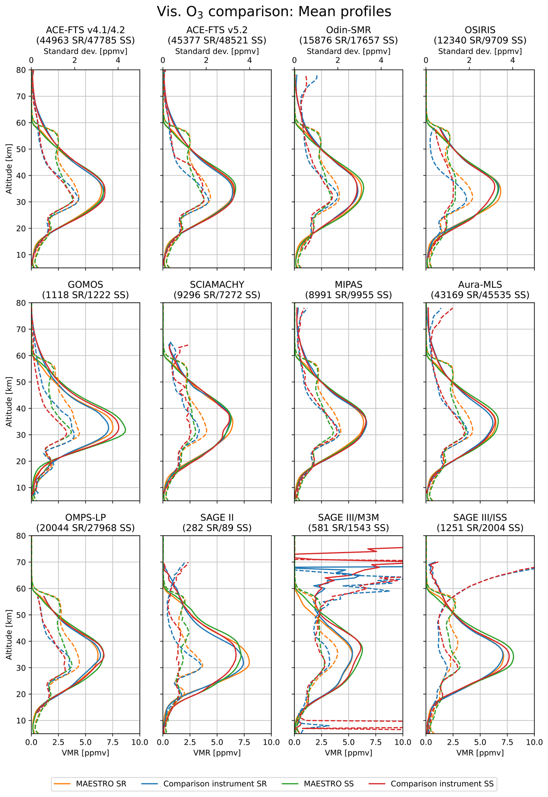
Figure 1 Comparison of the mean MAESTRO sunrise (SR) and sunset (SS) Vis-ozone profiles with mean coincident ozone profiles from the comparison instruments outlined in Sect. 2. The profiles from the comparison instruments are divided into whether they are coincident with MAESTRO sunrise or sunset measurements. The mean profiles are presented using the lower x-axis scale. The 1σ standard deviations of the profiles are shown as dashed lines using the upper x-axis scale. Under each instrument name is the number of coincident measurement pairs found for the MAESTRO sunrise/sunset measurements.

Generally, the MAESTRO mean ozone profiles are found to peak between 30 and 40 km, in broad agreement with the comparison datasets, with a sharp drop off above 50 km that shows a faster decrease in ozone concentration with altitude than observed for most of the comparison datasets. Near the ozone peak, the MAESTRO mean profiles tend to be biased slightly high, compared with the coincident datasets, with the largest biases found in comparisons made with Odin-SMR, GOMOS, SAGE II, and sunset-coincident SAGE III/ISS measurements. Above about 50 km, the sharp decrease in MAESTRO ozone leads to a distinct low bias compared with the other datasets that extends to the top of the profiles. The standard deviation of the MAESTRO profiles peaks about 5 km below the mean stratospheric ozone maximum, and general agreement is found with respect to the shape and magnitude of these profiles with those from the coincident datasets up to about 35 km. Above this altitude, between approximately 40 and 55 km, the MAESTRO standard deviation profiles are near 2.5 ppmv, whereas most of the coincident standard deviation profiles are less than half of this value over this range. Between about 60 and 80 km, the standard deviation profiles of MAESTRO are near 0 ppmv, an underestimation of the standard deviation compared with most of the other instruments. Finally, for most of the mean profile sets, with the exception of the OSIRIS, SCIAMACHY, and SAGE II profiles, the sunset profiles tend to be somewhat larger than the sunrise data. This is particularly evident in the comparisons with the GOMOS, SAGE III/M3M, and SAGE III/ISS instruments. In contrast, for the standard deviation profile sets, the sunrise profiles are found to be generally larger than the sunset profiles. This supports the separation of the comparisons into sunrise and sunset subsets.

Good agreement is found between MAESTRO and both the ACE-FTS version 4.1/4.2 and version 5.2 datasets from the troposphere to 50 km. Above this altitude, the MAESTRO and ACE-FTS profiles diverge, with the MAESTRO profiles yielding lower ozone up to the top of the profile. With the exception of the ACE-FTS v5.2 sunset profiles, the MAESTRO standard deviation is found to be larger than that of ACE-FTS between 30 and 60 km. The largest differences in these standard deviation profiles occur around 55 km, where the ACE-FTS v5.2 sunset profile values are also found to fall to lower values than the corresponding MAESTRO profile. Above 60 km, the near-0 ppmv MAESTRO standard deviation profiles are smaller than those profiles from ACE-FTS. Minimal differences are observed between comparisons made against the two versions of ACE-FTS. The comparisons with MIPAS are largely similar to those with ACE-FTS, with the two mean MIPAS ozone profiles overlapping significantly with each other and with the two mean MAESTRO ozone profiles below 50 km and showing similar standard deviation profiles to those observed with ACE-FTS. However, above 65 km, the MIPAS standard deviation profiles are found to be significantly larger than those observed for ACE-FTS or MAESTRO.

Generally good agreement is found with the SCIAMACHY, Aura-MLS, and OMPS-LP comparisons. However, only Aura-MLS reaches to the top of the MAESTRO profile; thus, the other two aforementioned instruments cannot be used to assess the representation of mesospheric ozone from MAESTRO. The profiles from Aura-MLS differ from those from MAESTRO by about 0.5 ppmv in the middle stratosphere; however, a more pronounced difference is visible between the mean sunrise- and sunset-coincident profiles, which are found to differ from each other to a greater extent than for the previously discussed datasets. In the mesosphere, the Aura-MLS comparisons are found to be similar to those made with MIPAS, with larger ozone standard deviation and slightly larger mean ozone values over this range than observed with ACE-FTS and MAESTRO. For the comparisons with SCIAMACHY, the largest differences in the mean ozone profiles are found just below the stratospheric ozone maximum, where MAESTRO is found to yield larger ozone VMRs by about 0.5 ppmv. Other than that, the two datasets are found to broadly agree between approximately 15 and 55 km. Lastly, the coincident OMPS-LP profiles are found to yield smaller mean VMRs than MAESTRO between 25 and 33 km and similar or slightly larger mean VMRs between 33 and 40 km, but overall good agreement is found through most of the profile, similar to that observed for the previous two datasets. Notable across the six sets of comparisons discussed so far is that the comparison datasets are from those least likely to be affected by sampling biases, due to the density of their sampling or their shared line of sight with MAESTRO, reinforcing the good agreement found with the MAESTRO Vis-ozone product.

From about 15 to 50 km, SAGE III/M3M is found to be in generally good agreement with MAESTRO; however, there is a large difference of about 1 ppmv observed between the sunrise and sunset sets of profiles that exceeds the differences observed for the aforementioned datasets. In the lower and middle stratosphere, it is expected that the sunrise and sunset profiles should generally agree with each other due to the small diurnal cycle of ozone at these altitudes. Thus, the observed difference between the sunset and sunrise profiles is likely influenced by some form of sampling bias associated with the sparse coverage and few coincidences found between MAESTRO and SAGE III/M3M. Outside of the stratosphere, the SAGE III/M3M profiles are found to be highly variable, with large oscillations in the mean SAGE III/M3M profiles below 10 km and above 60 km, which are accompanied by large jumps in the SAGE III/M3M standard deviation profiles and exponential growth in these profiles at high altitudes. These features are not reflected in MAESTRO data, nor in the other comparison datasets.

Somewhat similar agreement is found with Odin-SMR and OSIRIS, with both comparison datasets yielding less ozone than MAESTRO near the stratospheric ozone maximum. Around this maximum, the comparison profiles are typically within about 0.5 ppmv of those from MAESTRO. However, in the comparisons made with OSIRIS, there is an additional difference of about 0.5 ppmv near this peak between the sunrise and sunset profiles, with the sunrise measurement profiles yielding the larger concentrations. As with the SAGE III/M3M comparisons, this indicates the potential for sampling bias to play a role in the OSIRIS comparisons; however, given the greater degree of agreement between the sunrise and sunset profiles observed here, compared with those for the SAGE III/M3M comparisons, it is likely that it is a more limited effect. Further from the ozone peak, good agreement is found with MAESTRO and these two datasets, with the comparisons made with OSIRIS yielding the better agreement below 25 km and above 40 km. Above 60 km, the Odin-SMR mean and standard deviation profiles are similar to those from MIPAS and Aura-MLS, which reinforces the underestimation of ozone and ozone variability by MAESTRO above the stratosphere. The OSIRIS profiles do not extend up to 80 km, so they cannot be used to assess the agreement of mesospheric ozone.

The remaining datasets all show larger differences from MAESTRO as well as generally larger differences between their sunset and sunrise profiles that potentially arise from sampling biases. Beginning with GOMOS, comparisons with MAESTRO indicated that the latter has larger ozone values than the former, often in excess of 0.5 ppmv between 20 and 50 km, with the four profiles spread apart by approximately 2.5 ppmv. Between 60 and 70 km, the GOMOS profiles have larger ozone concentrations than MAESTRO, by up to about 1.2 ppmv, in closer agreement with what was observed for many of the prior comparisons. Despite the disagreement in magnitude over much of the mean profiles, the GOMOS comparisons share many profile features with those comparisons already touched upon. A similar spread in profiles is observed with the SAGE III/ISS comparisons, albeit with a maximum spread of only 1.5 ppmv, as opposed to 2.5 ppmv, near 35 km. As with GOMOS, SAGE III/ISS is found to have better agreement with MAESTRO for sunrise measurements than sunset measurements, with the pair of mean sunset profiles also having been found to have larger maximum ozone VMRs. The SAGE III/ISS standard deviation profiles are found to increase exponentially above 55 km, reaching the largest values of any of the measurement datasets assessed. Only the SAGE III/M3M standard deviation profiles are found to yield similar exponential growth in their standard deviation profiles at these high altitudes.

Lastly, significant disagreement is observed with the SAGE II comparisons, which possess features in their mean comparison profiles not seen with the other comparisons. The source of this disagreement is likely due to the limited number of comparisons that were possible between the SAGE II and MAESTRO datasets. These two datasets had the shortest overlap period, and only 371 comparisons could be made for the Vis-ozone product, nearly an order of magnitude fewer comparisons than for the dataset with the next fewest coincident measurements. Thus the agreement, or lack thereof, between MAESTRO and SAGE II should be treated with a degree of caution. Addressing the comparisons, it is found that the MAESTRO Vis-ozone product is larger than that from SAGE II between 20 and 50 km by as much as 0.8 ppmv. Additionally, the sunrise-coincident profiles are found to possess larger ozone concentrations than the sunset profiles by about 1 ppmv in the middle stratosphere. Unlike other datasets, the ozone peak occurs at a lower altitude for the sunrise comparisons than the sunset comparisons. The SAGE II sunset standard deviation profiles are found to remain around 1 ppmv from 20 to 45 km, dropping to nearly half of this value around 55 km, and finally increasing to 1 ppmv above 60 km alongside the SAGE II sunrise standard deviation profile. This last increase is found to be similar to what is observed for the sunset SCIAMACHY profiles.

4.1.2 Comparison metrics

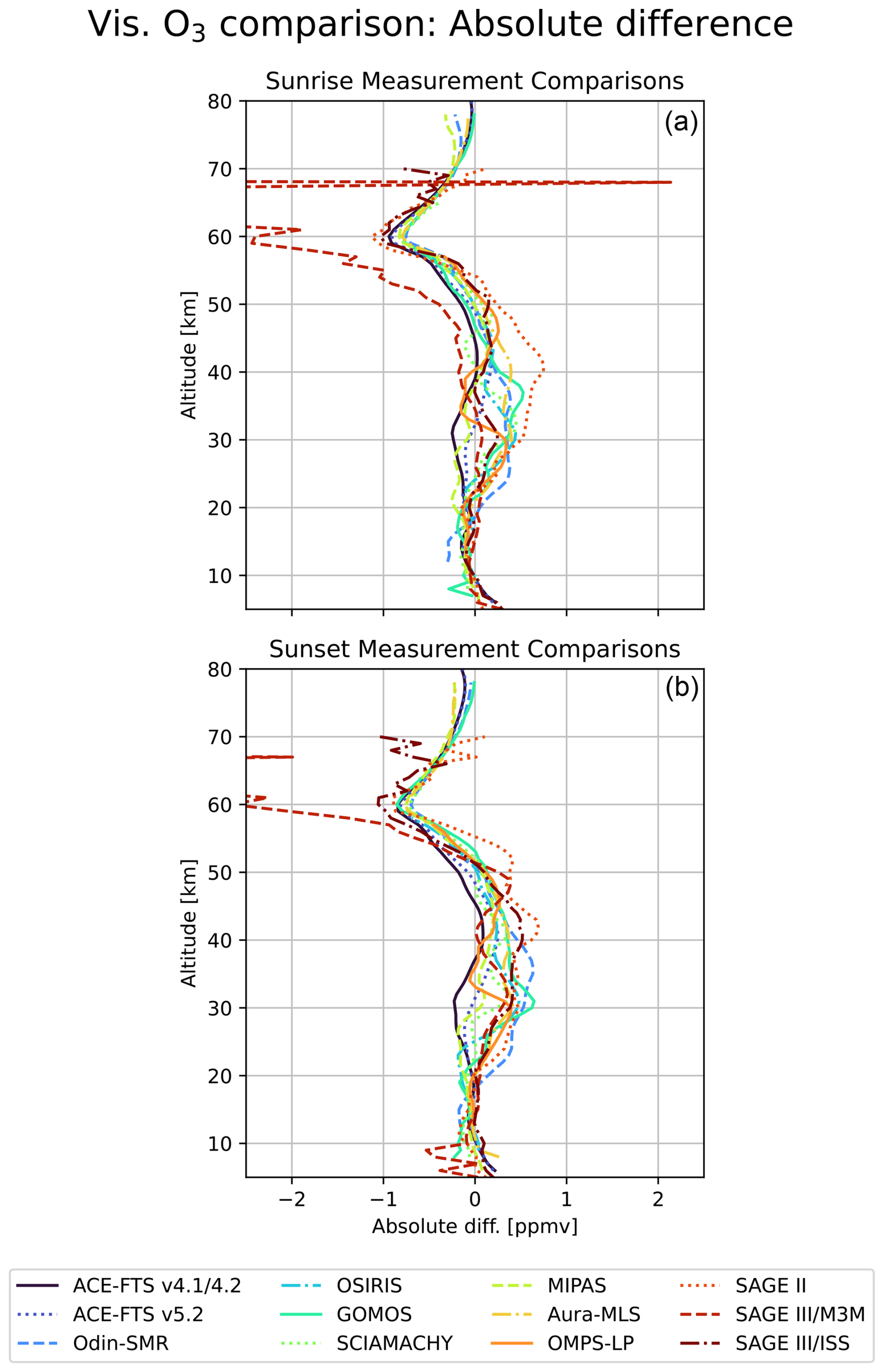
Figure 2 Mean absolute difference between MAESTRO (a) sunrise and (b) sunset Vis-ozone measurements and coincident ozone profiles from the comparison instruments outlined in Sect. 2.

Figure 3 Same as Fig. 2 but for the relative difference.

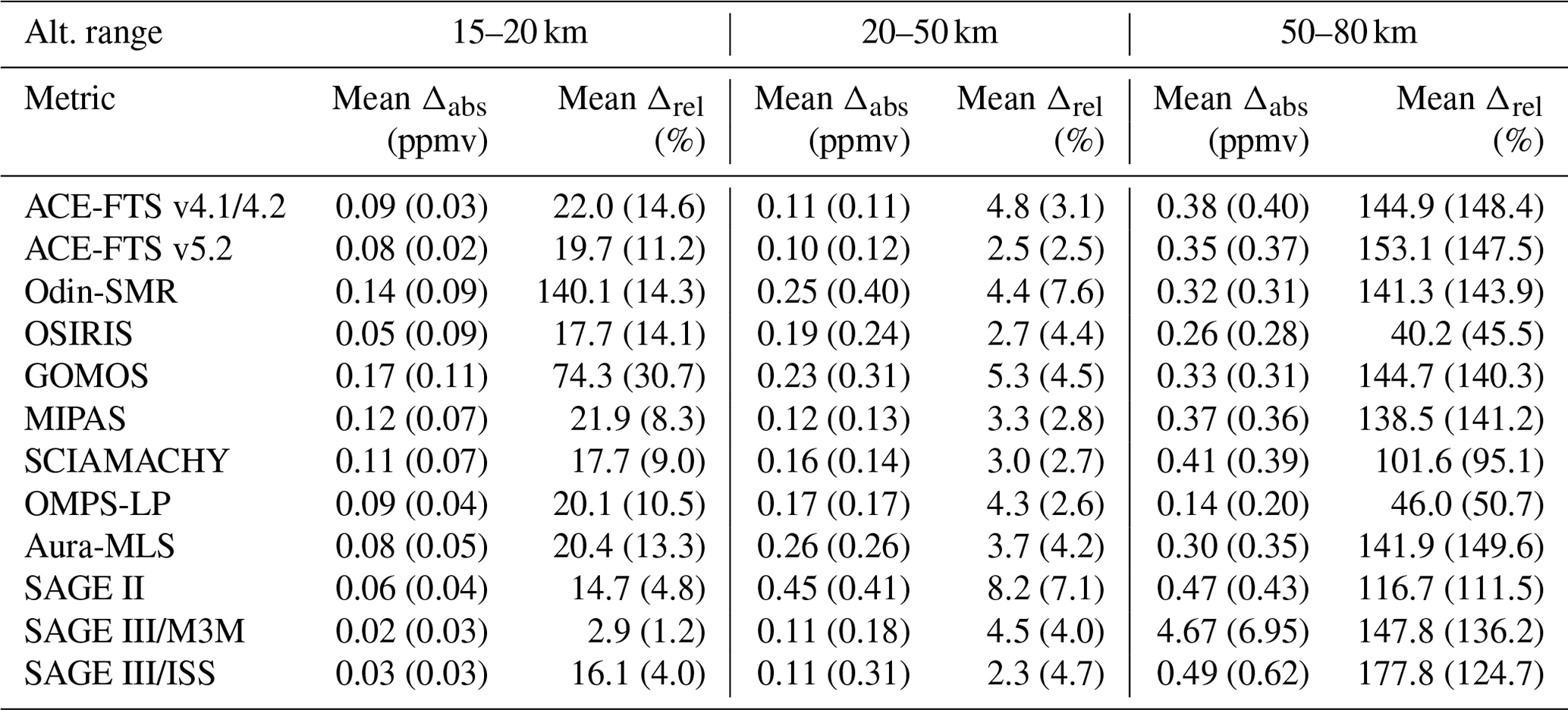
Table 2 Mean unsigned absolute (Δ_abs) and relative (Δ_rel) differences calculated between MAESTRO Vis-ozone sunrise (sunset) measurements and coincident measurements from the comparison datasets shown in the first column, averaged over three altitude ranges (Alt. range) covering 15–20 km, 20–50 km, and 50–80 km. This profile-averaged metric was calculated using the unsigned magnitude of the differences to avoid oppositely signed values cancelling.

Having addressed the general profile properties from each dataset, focus can turn to the comparison metrics outlined in Sect. 3. Figures 2 and 3 show the respective absolute and relative differences between the MAESTRO sunrise and sunset measurements and those measurements coincident with these from the other 12 datasets. From these comparisons, it is found that MAESTRO Vis-ozone shows generally good agreement with the comparison datasets between approximately 20 and 50 km, with generally similar agreement for both the sunrise and sunset measurements. These comparisons indicate that MAESTRO Vis-ozone is generally biased high between 20 and 50 km, with the only comparisons consistently indicating otherwise being those made with ACE-FTS version 4.1/4.2 and with the MIPAS sunrise-coincident measurements. Between 50 and 80 km, a low bias is found for the MAESTRO data, as the MAESTRO concentrations fall to near 0 ppmv by about 55 km. Taken with the extremely low standard deviation for MAESTRO over this range, this suggests that the MAESTRO retrieval may be over-constrained in the mesosphere, leading to the partitioning of ozone into the stratosphere and contributing to the high bias observed there. Below 20 km, the profile comparisons show small absolute differences but large relative differences with high variability, rendering comparisons over this span spurious, especially when coupled with the high uncertainty that many of the comparison datasets have at low altitudes.

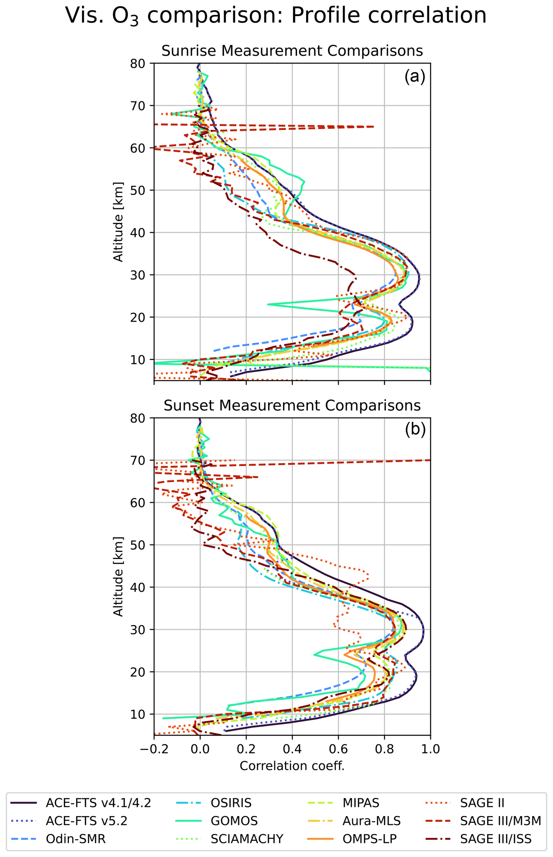
Figure 4 Pearson correlation coefficient between the MAESTRO (a) sunrise and (b) sunset Vis-ozone measurements and coincident ozone profiles from the comparison instruments outlined in Sect. 2.

Focusing between 20 and 50 km, where the overall closest agreement is observed, MAESTRO measurements agree best with ACE-FTS version 4.1/4.2, ACE-FTS version 5.2, and MIPAS, which have averaged absolute differences over this vertical range for sunrise (sunset) measurements of 0.11 (0.11) ppmv, 0.10 (0.12) ppmv, and 0.12 (0.13) ppmv, respectively. This profile-averaged metric was calculated using the unsigned magnitude of the differences to avoid oppositely signed values from cancelling. These differences translate into profile-averaged relative differences of 4.8 (3.1) % for ACE-FTS version 4.1/4.2, 2.5 (2.5) % for ACE-FTS version 5.2, and 3.3 (2.8) % for MIPAS over this range. Very good agreement is also found with OSIRIS, SCIAMACHY, OMPS-LP, SAGE III/M3M, and sunrise measurements from SAGE III/ISS. Comparisons with Odin-SMR and SAGE II show the poorest agreement over this range, with average absolute differences of 0.25 (0.40) ppmv and 0.45 (0.41) ppmv, respectively, for sunrise (sunset) comparisons; however, these values translate into average relative differences of 4.4 (7.6) % for Odin-SMR and 8.2 (7.1) % for SAGE II, indicative that the MAESTRO Vis-ozone product is still generally in good agreement in the range of 20 to 50 km. Despite this, the agreement with SAGE II should still be treated with a degree of caution due to the extremely limited number of comparisons that were possible with the two datasets.

Between 15 and 20 km, near the lower bounds of many of the instrument measurements, most of the datasets continue to show reasonable agreement with MAESTRO, with most of the sunrise (sunset) MAESTRO measurements agreeing with the comparison datasets to within 22.0 (14.6) %. The main exceptions to this are the comparisons with the GOMOS instrument, which show values differing by 74.3 (30.7) % on average for sunrise (sunset) comparisons, and the sunrise Odin-SMR comparisons, which show a 140.1 % difference on average. Below this altitude range, the comparisons show significant disagreement, often displaying differences at particular altitudes in excess of 50 %. Similarly, above 50 km, the comparisons generally show considerable disagreement, with differences reaching over 100 %.

These results indicate that there is excellent agreement between MAESTRO and the other datasets between 20 and 50 km, good agreement from 15 to 20 km, and poor agreement in the troposphere and mesosphere. The absolute and relative differences are summarized in Table 2 for three altitude regimes, corresponding to 15–20 km (where generally fair agreement is found), 20–50 km (where excellent agreement is found), and 50–80 km (where poor agreement is found).

Lastly, the correlation between the MAESTRO and comparison datasets is shown in Fig. 4. Here, we define good correlation as having a correlation coefficient greater than 0.7 and moderate correlation as having a coefficient between 0.5 and 0.7. Across the 12 datasets, the highest correlation is observed between 15 and 40 km, where, with the exception of SAGE II sunset-coincident measurements and SAGE III/ISS sunrise-coincident measurements, the datasets have profile-averaged correlations with MAESTRO of at least 0.71. Outside of this range, the profile correlation coefficients fall to 0.5 between 10 and 15 km and between 40 and 45 km. At 50 km, most of the correlation coefficients are between 0.2 and 0.4, with the exception of SAGE III/M3M, SAGE III/ISS, and OSIRIS which are less than 0.2. As many of the comparison datasets can have spurious results near the troposphere, physical interpretations of the correlation coefficients at low altitudes are difficult. However, the drop in the correlation coefficients at and above 50 km indicates that the MAESTRO Vis-ozone product should only be used for scientific applications below this altitude, as found from the profile difference comparisons. The low correlation at high altitudes, coupled with the poor agreement at high altitudes, provides evidence that the extremely low ozone at high altitudes is likely due to a retrieval artifact, as this feature is not seen in the other datasets.

4.2 UV-ozone

The comparisons between the MAESTRO sunrise and sunset UV-ozone data and the diurnally scaled (where required) coincident ozone measurements are shown in Figs. 5–8. Due to the limited period of viable MAESTRO UV-ozone measurements, from the start of the mission until December 2009, there are significantly fewer coincident measurements for this set of comparisons than for the Vis-ozone comparisons. Additionally, both OMPS-LP and SAGE III/ISS began operations after the cutoff date for the MAESTRO UV-ozone product; thus, no coincidences are found with these two datasets. Finally, a comparison of the MAESTRO Vis-ozone and UV-ozone profiles is shown in Fig. 9.

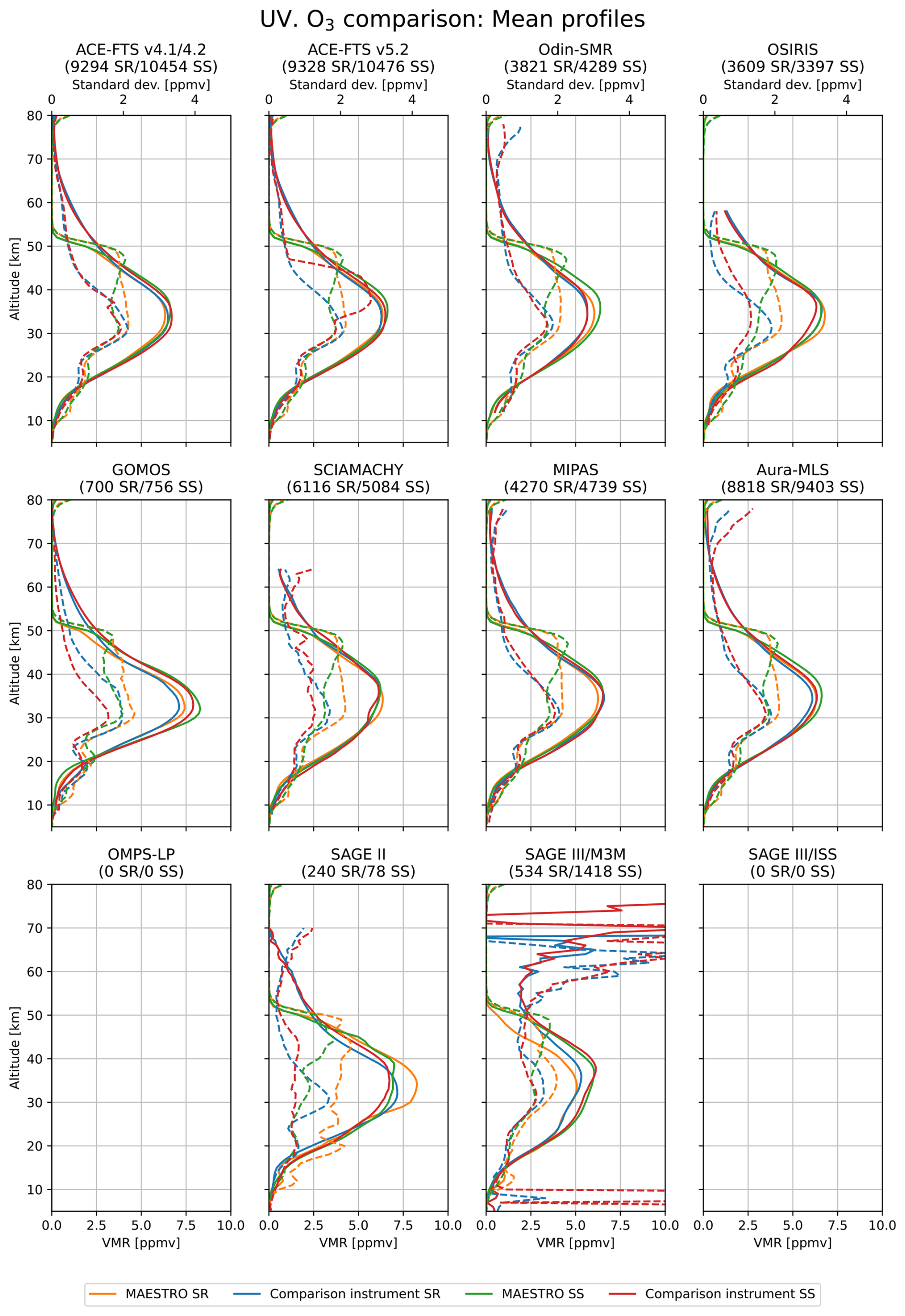
Figure 5 Same as Fig. 1 but for MAESTRO UV-ozone measurements. Note that there are no coincident measurements between the MAESTRO UV-ozone product and OMPS-LP and SAGE III/ISS.

4.2.1 Profile overview

Despite a more limited number of coincident profiles, the mean MAESTRO UV-ozone profiles, comparison profiles, and standard deviations profiles, all shown in Fig. 5, are extremely similar between 20 and 50 km to those for the Vis-ozone comparisons shown in Fig. 1. This similarity includes the small high bias previously observed for the MAESTRO dataset. Two main differences distinguish the sets of UV-ozone and Vis-ozone profiles. The first difference is found in the mean MAESTRO profiles near 50 km, where a much sharper decrease in ozone concentration is noted for the UV-ozone product than for the Vis-ozone product, with the VMR of ozone falling to near 0 ppmv by 55 km. The other main difference between the two products, as shown in Figs. 1 and 5, is the MAESTRO standard deviation between 30 and 60 km. In the Vis-ozone product, the standard deviation profiles across this range generally peak at around 2 ppmv at 30 km, decrease to around 1.3 ppmv between 40–45 km, and remain constant up to about 55 km before decreasing to near 0 ppmv at 60 km. In contrast, for the UV-ozone profile, the MAESTRO sunrise standard deviation profiles increase in magnitude from the troposphere up to 30 km, remain generally constant (near 2 ppmv) between 30 and 50 km, and finally decrease sharply to near 0 ppmv around 55 km. The sunset profiles share the same increasing and decreasing behaviour as the sunrise profiles below 30 km and above 50 km, respectively, but the standard deviation profiles are found to peak near 45 km. Both sets of profiles indicate that, despite similar profiles, the UV product is more variable than the Vis-ozone product over much of the stratosphere.

As with the Vis-ozone product, the UV-ozone product also underestimates the variability in the mesosphere compared with the comparison datasets. The observed low variability in the mesosphere, coupled with the small mean VMRs in the region, can be interpreted as the result of the ozone retrieval being over-constrained to small VMR values over this span, as suggested for the Vis-ozone product. This then can cause the retrieval to partition ozone, whose existence is derived from the optical depth spectra, into less-constrained retrieval levels. The high variability observed for MAESTRO in the stratosphere provides evidence that the MAESTRO retrieval is far less constrained in this region, which allows for ozone to be readily partitioned into the stratosphere by the retrieval. This, in turn, might be the cause of the small high bias observed for the MAESTRO UV-ozone product. However, given the agreement between the datasets, it is likely that this has only a minor effect on the stratospheric ozone concentrations, allowing for the conclusion that the UV-ozone product is generally well constrained only below about 50 km and should be used cautiously above this point.

Figure 6 Same as Fig. 2 but for MAESTRO UV-ozone measurements.

Figure 7 Same as Fig. 3 but for MAESTRO UV-ozone measurements.

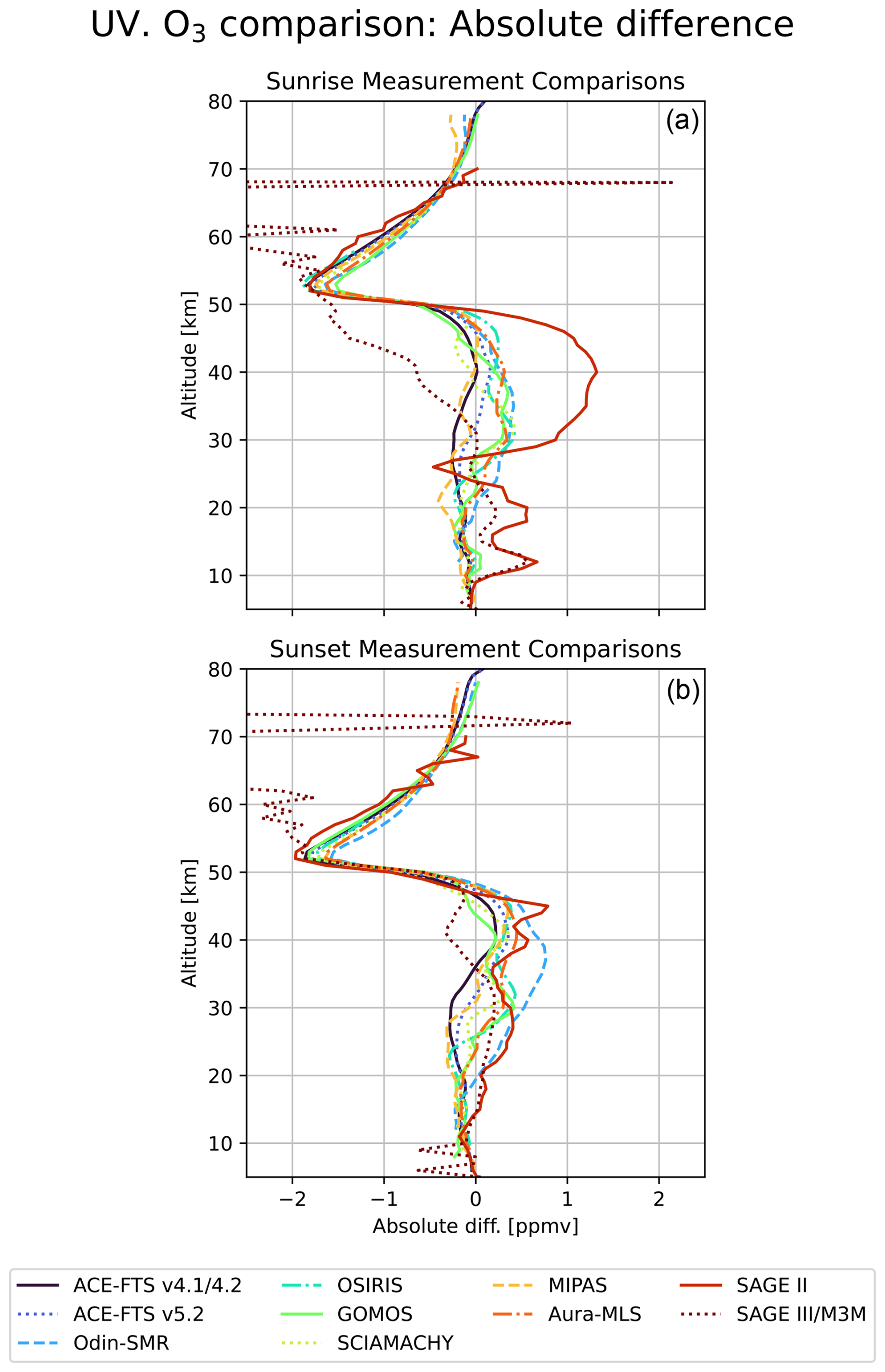
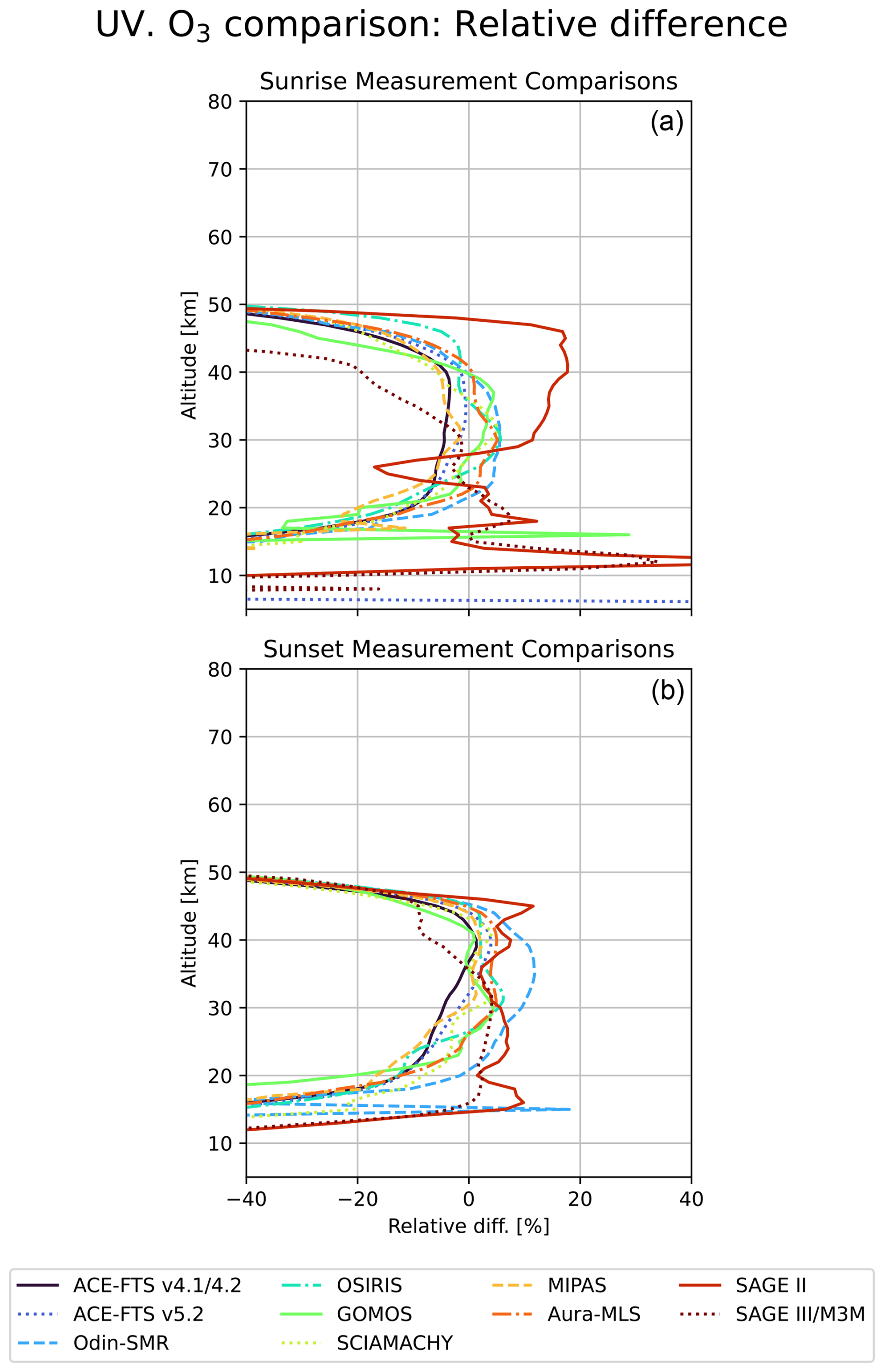
4.2.2 Comparison metrics

Having addressed the main differences in the mean and standard deviation profiles from those discussed in Sect. 4.1, attention can turn to the direct comparisons between dataset pairs. As with the Vis-ozone product, the MAESTRO UV-ozone absolute and relative differences, shown in Figs. 6 and 7, respectively, show the best agreement in the stratosphere, with MAESTRO yielding generally higher ozone concentrations than the comparison instruments. Examining the relative difference plots, it is clear that the vertical range for which good agreement is found is somewhat narrower for the UV product than the Vis-ozone product, with the closest agreement between the datasets found between approximately 20 and 45 km. Within this range, the best agreement is found with ACE-FTS, with version 4.1/4.2 differing by 0.15 (0.19) ppmv and version 5.2 differing by 0.12 (0.20) ppmv; with GOMOS, with differences of 0.17 (0.16) ppmv; and with SCIAMACHY, with differences of 0.17 (0.16) ppmv, on average, from sunrise-coincident (sunset-coincident) profiles. The relative differences also reflect this good agreement, with average sunrise (sunset) differences of 5.7 (4.2) % for ACE-FTS version 4.1/4.2, 3.6 (4.0) % for ACE-FTS version 5.2, 4.8 (3.3) % for GOMOS, and 5.0 (2.8) % for SCIAMACHY. Due to greater differences near the stratospheric ozone maximum, Aura-MLS is found to have a smaller average relative difference than most of these comparisons, 2.8 (4.2) % during sunrise (sunset), while also having larger average absolute differences, 0.21 (0.25) ppmv. This mixed behaviour emphasizes the need to include both difference metrics in this analysis.

Considering all of the datasets within the 20 to 45 km range, the majority of the comparisons have average absolute differences of between 0.12 and 0.30 ppmv for the sunrise comparisons and between 0.16 and 0.34 ppmv for the sunset comparisons. The exceptions to this are the sunrise SAGE II comparisons, which have an average absolute difference of 0.83 ppmv, and the sunset Odin-SMR comparisons, with an average difference of 0.49 ppmv. These two datasets also show the highest relative differences of 11.9 % and 7.6 %, respectively, on average; however, these average differences still indicate reasonable agreement. The other datasets show span-averaged relative differences of between 2.8 % and 10.8 % for sunrise comparisons and between 2.8 % and 5.2 % for sunset comparisons, inferring that many of the datasets are in excellent agreement with MAESTRO UV-ozone in the stratosphere. As with the Vis-ozone product, the fewest coincident measurements for the UV-ozone product are found with SAGE II, with only 318 coincident profiles found overall. Thus, the comparisons with SAGE II should continue to be treated with a degree of caution.

In the lower stratosphere, between 15 and 20 km, the MAESTRO UV-ozone comparisons show larger relative differences, with the average difference of most of the datasets falling between 5.0 % and 33.0 %. The best mean agreement is noted for comparisons with SAGE II and SAGE III/M3M measurements, which have a relative difference of 5.0 (7.3) % and 3.7 (1.9) % during sunrise (sunset), respectively. The GOMOS sunset-coincident measurements show the largest average relative difference of 63.7 %. Even with the exception of this last set of comparisons, generally poor agreement can be found with the majority of the datasets in this altitude range, indicating that the UV-ozone product should be used with caution here. Below 15 km, the disagreement between datasets is larger, with many sets of comparisons exceeding 50 % relative differences; similarly, above 45 km, many sets of comparisons exceed differences of 150 %. Altogether, this indicates that the MAESTRO UV-ozone dataset is best used as a stratospheric product. As with the Vis-ozone comparisons, the absolute and relative differences for the UV-ozone comparisons are summarized in Table 3 for three altitude regimes, corresponding to 15–20 km, 20–45 km, and 45–80 km, chosen to highlight the properties of this product.

Table 3 Same as Table 2 but for MAESTRO UV-ozone.

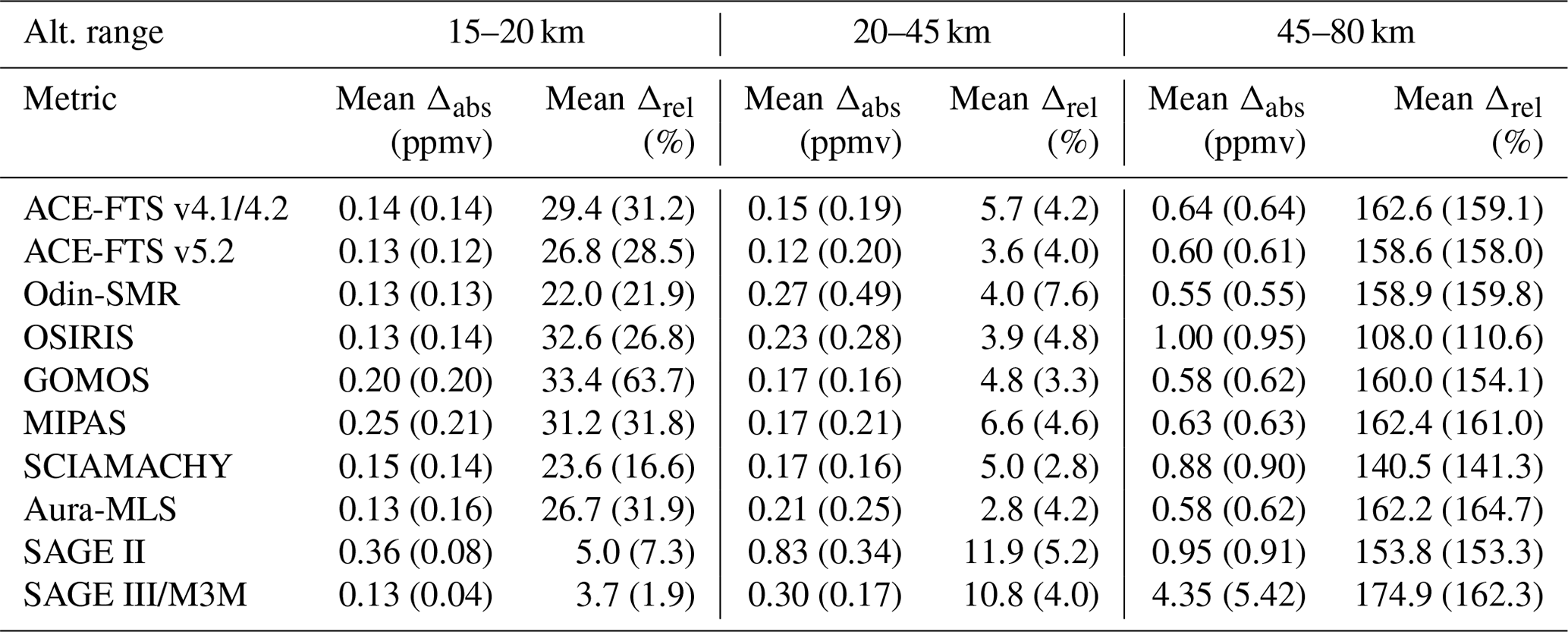
The correlation between the coincident measurements is shown in Fig. 8. Across the majority of the comparisons, the largest correlation coefficients are found between approximately 15 and 35 km. Within this range, the best profile-averaged correlation is found with ACE-FTS, with both versions yielding coefficients of 0.88 for sunrise-coincident measurements and above 0.87 for sunset measurements. The lowest average correlation coefficients in this range come from comparisons with SAGE II sunrise measurements, which have an average value of 0.54; with GOMOS sunset measurements, which have an average value of 0.67; and with Odin-SMR, which has an average coefficient of 0.66 (0.69) during sunrise (sunset). Due to the sparse sampling of the first two datasets, there is a strong likelihood that those comparisons are influenced by sampling bias, contributing to the poor correlation observed. The remaining datasets show average correlation coefficients over this range between 0.72 and 0.79 for sunrise-coincident measurements and between 0.70 and 0.79 for sunset-coincident measurements. While the coefficient correlations are somewhat less than for the Vis-ozone product, the correlation coefficients over this range show that the majority of the datasets are in good agreement with MAESTRO over this range. Outside of the 15 to 35 km range, the correlation coefficients quickly fall to low values, dropping to below 0.5 for the majority of the datasets below 13 km and above 42 km. Greater differences are noted with the UV-ozone product between the sunrise and sunset correlation coefficients, with the latter tending toward lower correlation values. Combined with the narrower range of good agreement, the measurement correlation shows that the UV-ozone product should be treated more cautiously than the Vis-ozone product.

4.2.3 Comparison of MAESTRO Vis-ozone and UV-ozone

In addition to the comparisons of the two MAESTRO ozone products against other datasets, they can also be compared against each other. As the two products are retrieved independently, this intercomparison allows for an examination of the consistency of the ozone products while also removing the influence of geophysical variability. Ahead of this direct product intercomparison, it is also worth noting that a similar minimization of the impact of geophysical variability occurs in the comparisons made between the MAESTRO products and ACE-FTS as the two instruments share a line of sight and measure at the same time using the same observational geometry, allowing direct comparisons to more directly assess the instrumentation and retrieval technique(s). Thus, the excellent agreement observed for both MAESTRO ozone products with ACE-FTS gives confidence in the data treatment and reinforces the viability of these instruments and their ozone data products.

Direct comparisons of the MAESTRO Vis-ozone and UV-ozone products are shown in Fig. 9. Starting with the mean profiles, the sunrise and sunset profiles are found to be in good agreement from the troposphere up to about 47 km, with the Vis-ozone product having a slightly larger ozone concentration over this range. Above about 47 km, there is a sharp decrease in the UV-ozone mean concentration, such that the UV product falls to near 0 ppmv by 55 km. In contrast, the Vis-ozone product more gradually decreases from the stratospheric ozone maximum, only reaching concentrations near 0 ppmv at around 60 km. The UV-ozone product is also found to have significantly larger standard deviation profiles between 30 and 53 km, while the standard deviation profiles of the Vis-ozone product are larger between 53 and 60 km.

Turning to the absolute difference, only small differences are noted below about 47 km and above 60 km; moreover, within this range, the MAESTRO Vis-ozone is found to be larger than the UV-ozone product due to the differences in behaviour observed with altitude for the two products. The relative difference profiles largely reflect these absolute differences, with the exception of large differences noted below about 20 km that can be at least partially attributed to the small VMR of ozone at low altitudes that leads small absolute differences to result in large relative differences. Finally, the correlation coefficients are found to be high between about 15 km and either 35 km (sunset) or 40 km (sunrise), largely similar to the correlation coefficients shown for the UV-ozone product in Fig. 8.

The loss of signal from the UV channel of MAESTRO likely contributes to the observed differences between the two MAESTRO ozone products. As stated above, the gradual buildup of an unknown contaminant reduced the throughput of the MAESTRO UV channel, such that there was insufficient signal for the retrieval of viable products from this channel after 2009. However, this was a gradual change over time, rather than a sudden event, and the 2009 end date is empirically determined based on the quality of data retrieved from MAESTRO measurements. As such, there was a gradual decrease in the quality of the products over time, and, although the version 4.5 UV products have been thoroughly vetted, this degradation may contribute to the observed differences between the UV-ozone and the Vis-ozone. The larger standard deviation profiles of the former support a gradual change in the product over time. Between this gradual loss, the sharper decrease in ozone above 50 km, and the somewhat more limited range over which good agreement and high correlation is found between the MAESTRO UV-ozone product and that of the other datasets, it is found that the Vis-ozone product is better suited for use in scientific applications.

Figure 8 Same as Fig. 4 but for MAESTRO UV-ozone measurements.

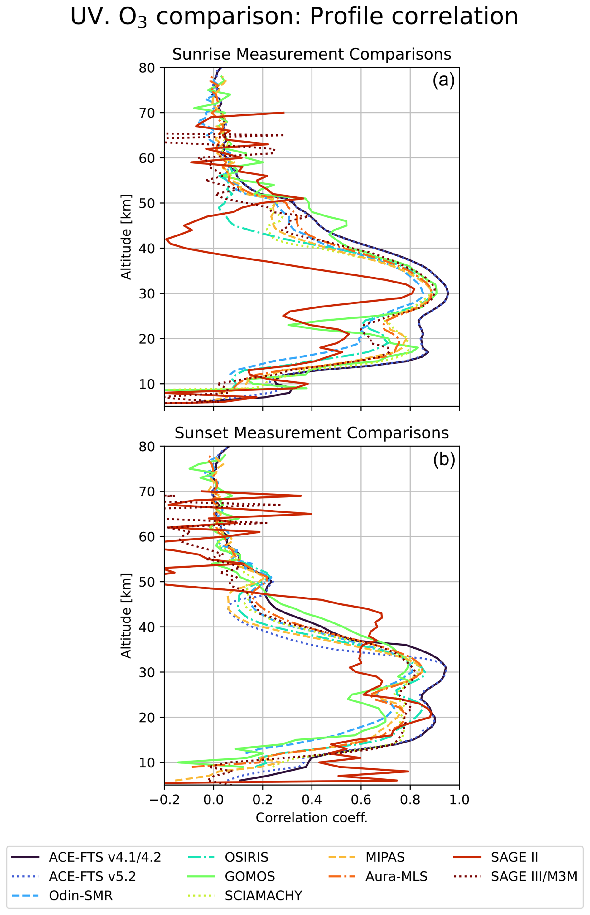
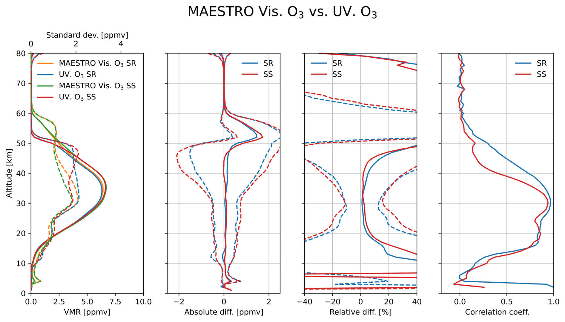
Figure 9 Comparison of the MAESTRO sunrise (SR) and sunset (SS) Vis-ozone profiles with the MAESTRO UV-ozone profiles. From left to right, the mean sunrise and sunset profiles, the absolute difference, relative difference, and correlation coefficient are shown. The mean profiles are presented using the lower x-axis scale, with the 1σ standard deviations of the profiles shown as dashed lines using the upper x-axis scale.

Figure 10 Same as Fig. 1 but for MAESTRO UV NO₂ measurements.

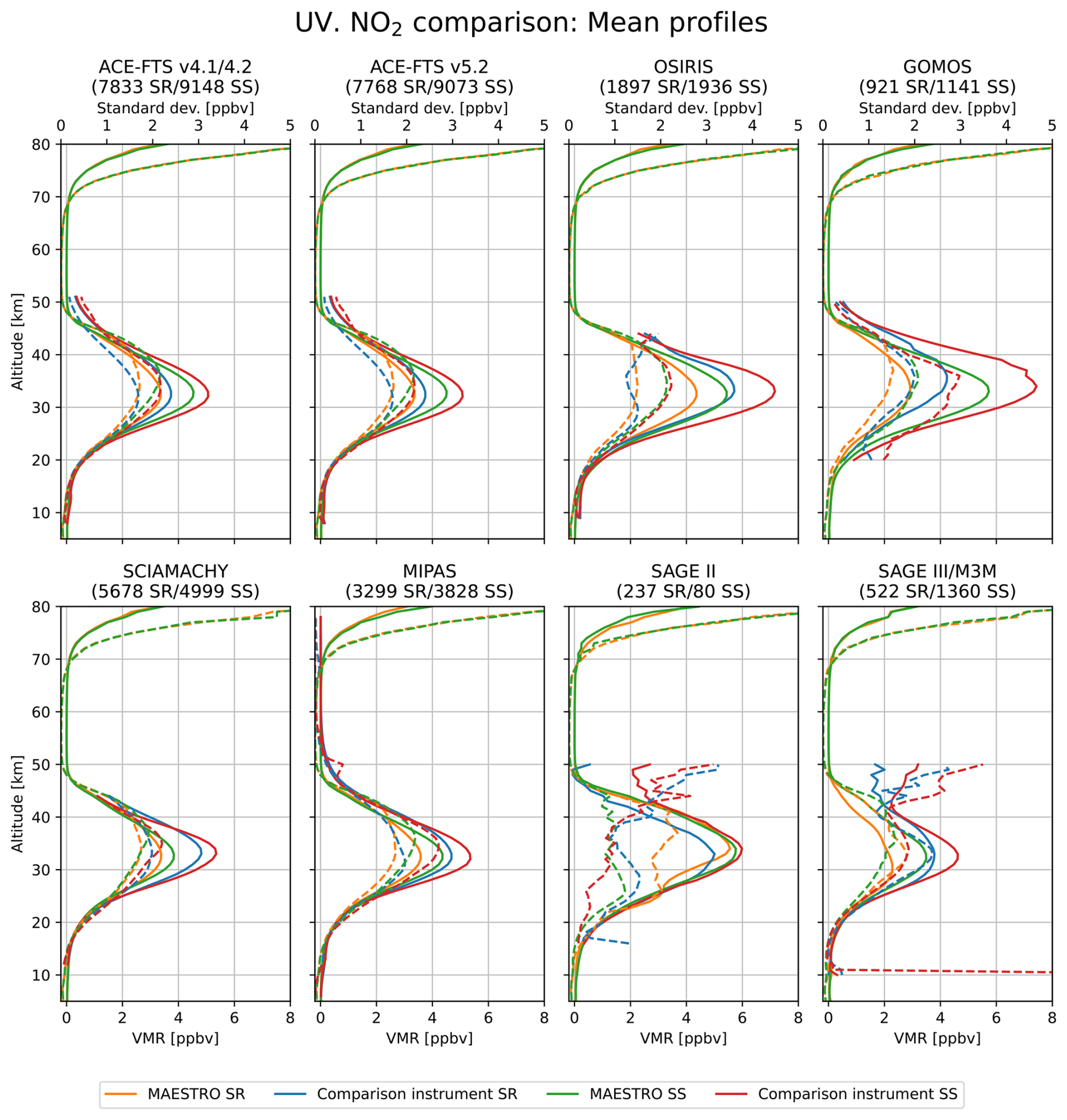
4.3 UV NO₂

Comparisons between the MAESTRO sunrise and sunset NO₂ data against the diurnally scaled (where required) coincident measurements from the other datasets are shown in Figs. 10–13. As with the UV-ozone data, the MAESTRO NO₂ measurements are only viable for a portion of the MAESTRO operational period, in this case, from the start of the mission through to June 2009. As a result of this, as well as the fact that not all of the datasets employed in this study have an NO₂ product, only eight sets of comparisons can be made, with none being made with Odin-SMR, Aura-MLS, OMPS-LP, or SAGE III/ISS.

4.3.1 Profile overview

The mean sunrise and sunset MAESTRO and coincident comparison profiles and their standard deviations are shown in Fig. 10. Across the eight sets of profiles, the shape of the mean NO₂ profile is generally consistent below approximately 45 km, with the mean profiles showing an increasing concentration with altitude from the troposphere up to a maximum near 35 km. Above this maximum, the NO₂ concentration begins to decrease with altitude; however, around 45 km, the datasets begin to differ from each other, with two datasets (OSIRIS and SCIAMACHY) truncating at this altitude, two sunset profiles (SAGE II and SAGE III/M3M) showing fairly fixed NO₂ concentrations with altitude, and the remaining profiles continuing to decrease with altitude. As for ozone, the MAESTRO NO₂ mean profiles show a sharper decrease in concentration with altitude than the comparison datasets, with this deviation occurring around 45 km. Here, MAESTRO NO₂ quickly decreases to near 0 ppbv, as does its standard deviation. Above 70 km, the MAESTRO profiles increase with altitude; however, only MIPAS has NO₂ measurements past 50 km, and this mesospheric feature is not observed in the MIPAS data.

Around the stratospheric NO₂ peak, large differences are found in the mean profile trace gas concentrations, with peak values ranging from just over 2 ppbv up to about 7.5 ppbv around 35 km. Along with the large spread in mean profile concentrations between the datasets, the sunrise and sunset profiles are found to consistently differ from each other for each of the datasets, with the latter yielding larger NO₂ VMR values throughout the majority of the stratosphere. Unlike for the ozone profiles, a more pronounced difference in the sunrise and sunset profiles due to the diurnal cycle of NO₂ is expected; however, the scale of these differences between the different sets of comparisons shows the potential for sampling biases to impact these comparisons in the less densely sampled, non-ACE-FTS datasets. Despite the variability in the mean profiles, all but one of the comparisons (SAGE II sunrise) indicate that MAESTRO NO₂ is biased low in the stratosphere compared with the other datasets. This low bias is most clearly illustrated in comparisons made with OSIRIS, GOMOS, and SCIAMACHY. The differing behaviour observed with the SAGE II sunrise NO₂ dataset can be at least partially attributed to the thermal shock that the instrument experiences during measurement events, which can be readily accounted for in sunset measurements but requires a correction to be applied for the sunrise measurements (Damadeo et al., 2013). Around the stratospheric NO₂ maximum, most of the datasets also display their largest standard deviations; however, there is some variation with respect to the exact altitude at which the largest values occur. Both of the SAGE II profiles, as well as the SAGE III/M3M sunset profile, show their largest standard deviation values between 40 and 50 km; however, this is likely associated with retrieval-boundary uncertainty effects and the aforementioned thermal shock for the former.

Figure 11 Same as Fig. 2 but for MAESTRO UV NO₂ measurements.

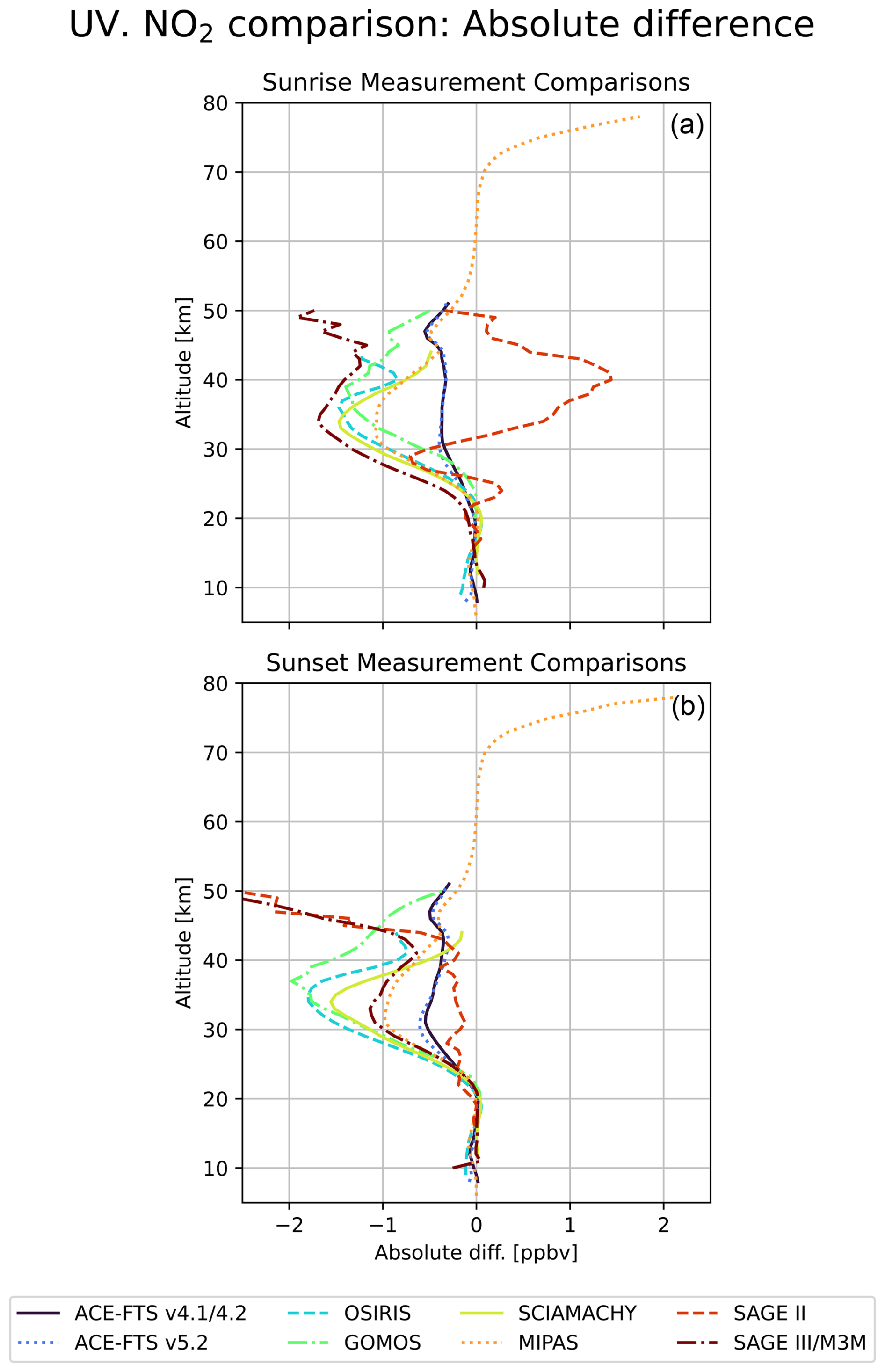
Despite the low bias of the mean MAESTRO profiles, the standard deviation profiles for the MAESTRO NO₂ product show general agreement in the stratosphere with those from the comparison instruments. Above 70 km, the MAESTRO dataset displays extremely large standard deviation values in association with the aforementioned mesospheric NO₂ feature, with standard deviation values in excess of 10 ppbv. This large upper atmospheric variability, coupled with the large NO₂ concentrations not observed elsewhere, indicates that this secondary NO₂ feature in the MAESTRO dataset might be an artifact caused by the retrieval. The exact cause of this is likely the over-constraint of the retrieval in the lower mesosphere, as observed with the ozone products from MAESTRO, coupled to an under-constrained region, namely, the span from 70 km upward, into which the NO₂ is partitioned.

Figure 12 Same as Fig. 3 but for MAESTRO UV NO₂ measurements.

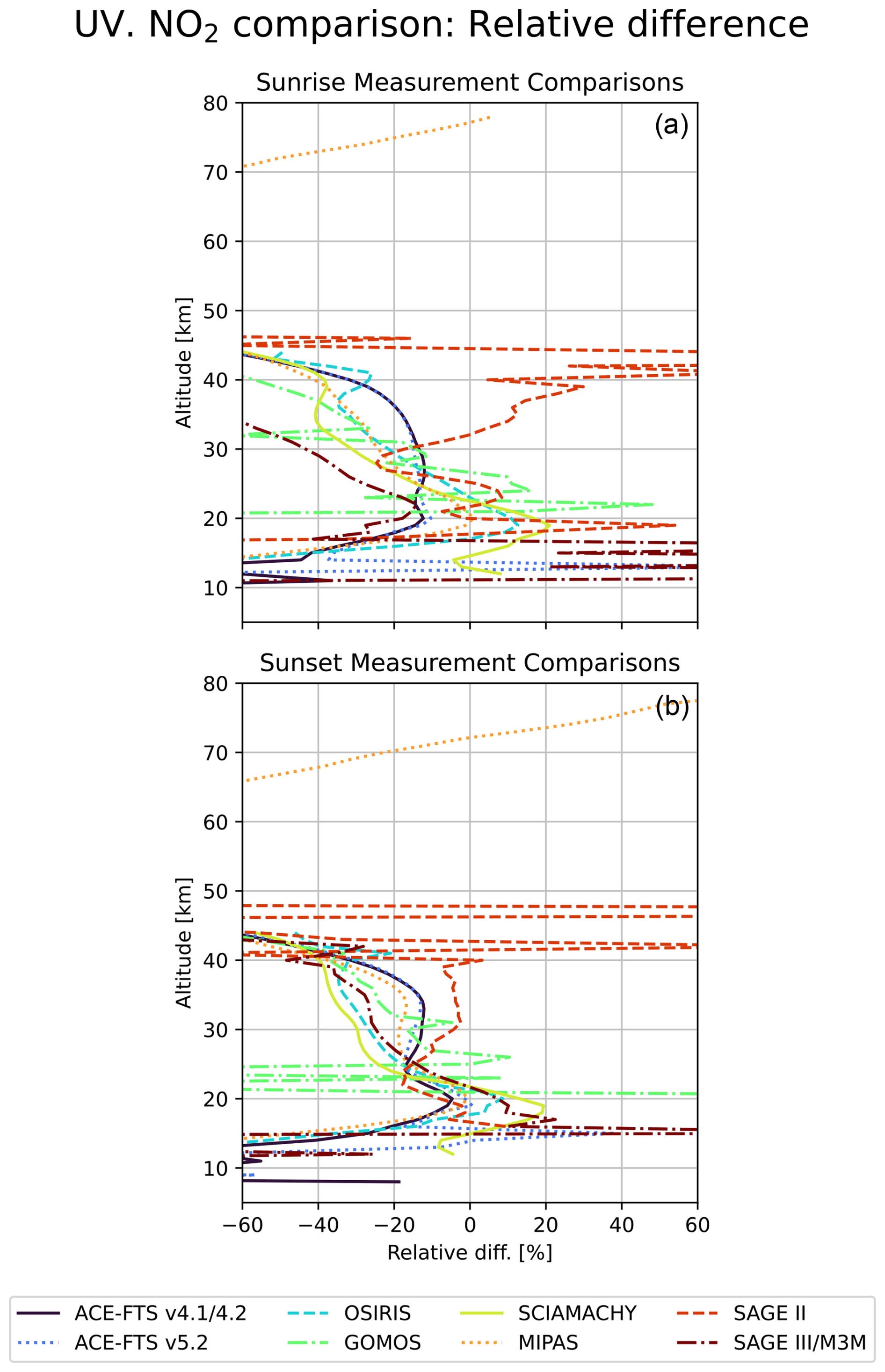
Focusing on the individual sets of comparisons, the best agreement is found between MAESTRO and the ACE-FTS version 4.1/4.2 and version 5.2 datasets. The NO₂ from all three datasets is found to peak at the same altitude in the stratosphere, and the sunset measurements are found to be about 1 ppbv larger than the sunrise measurements at this point for both sets of comparisons, which is expected given the diurnal cycle in NO₂. The standard deviation profiles from ACE-FTS and MAESTRO are also found to follow a similar shape, with the sunrise profiles peaking near the VMR maximum, while the sunset profiles peak closer to 37 km, showing a consistency in the representation of NO₂ between the datasets. However, despite these shared properties, there is a difference of about 0.3 ppbv between the mean MAESTRO and ACE-FTS profiles, which persists from about 28 km up to 40 km. The magnitude of this difference is unexpected given the shared line of sight of ACE-FTS and MAESTRO as well as results from preflight tests of the two instruments that showed agreement to within 0.5 % for measurements of NO₂ (Dufour et al., 2006). A factor contributing to this difference is likely the lack of temperature corrections for the MAESTRO data in the NO₂ retrieval. Additionally, while the MAESTRO mean NO₂ is found to be smaller than that of ACE-FTS, the standard deviation of the MAESTRO dataset is slightly larger than that of ACE-FTS, indicating that it is a more variable product.

Table 4 Same as Table 2 but for MAESTRO NO₂. Note that there are no data below 20 km for GOMOS, resulting in the empty entries in the table. Additionally, not all datasets reach up to 60 km; thus, where this is the case, the average is presented up to the maximum available altitude.

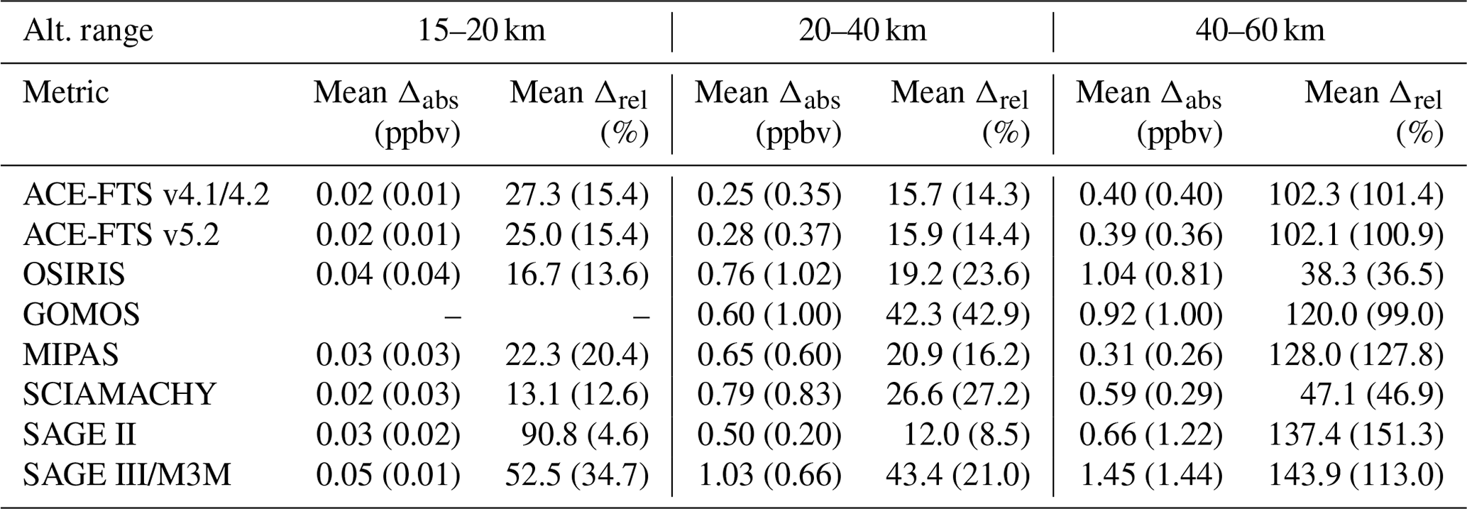
The GOMOS comparisons are generally similar to those with ACE-FTS, albeit with three main differences. The first difference is in the magnitude of the mean sunset NO₂ profile; both the GOMOS sunset profile and the MAESTRO sunset profile show higher NO₂ concentrations around the stratospheric NO₂ maximum, by about 2 and 1.5 ppbv, respectively, compared with the same type of profile from the ACE-FTS datasets. The second difference is in the location of the stratospheric NO₂ peak, with the two GOMOS profiles peaking approximately 2 km higher than those seen in the ACE-FTS comparisons. Despite this, the standard deviation profiles reach their maximum value at a higher altitude for the sunset profiles, as observed with ACE-FTS. The final difference is in the general agreement between the MAESTRO and GOMOS profiles, which shows a larger absolute difference over the stratosphere than what was observed for ACE-FTS, with differences near the stratospheric peak of 1.5–2 ppbv.

Broadly the OSIRIS, SCIAMACHY, and MIPAS comparisons share similar properties with each other, which differentiate these comparisons from those above. Most notably, for each of the comparison datasets, both the mean sunset and sunrise NO₂ profiles are found to be larger than both of the coincident profiles from MAESTRO, with an approximate 1–2 ppbv difference between the comparison and MAESTRO profiles around the stratospheric maximum. Despite this, the general relationship between the sunrise and sunset profiles, wherein the latter is larger than the former, is maintained in these comparisons. The three sets of comparisons also show some significant points of difference from each other. This includes the sunset profiles from the OSIRIS comparisons having larger mean VMR values (by 1–2 ppbv) than the MIPAS or SCIAMACHY comparisons and the sunrise standard deviation profiles from the OSIRIS comparisons having the smallest standard deviation profiles of the three. Additionally, the MIPAS dataset has NO₂ information up to 79 km, unlike the other comparison datasets; however, above 50 km, these retrieved values are consistently very small, unlike those of MAESTRO, showing no agreement with the MAESTRO high-altitude NO₂ feature.

Finally, the SAGE II and SAGE III/M3M comparisons are shown to differ significantly from what is seen with the other comparisons. Starting with the similarities with the other comparisons, the SAGE II and SAGE III/M3M mean profiles have larger NO₂ concentrations for the sunset measurements than for the sunrise, and the mean profiles show a peak in NO₂ at around 35 km. SAGE III/M3M shows larger NO₂ concentrations than MAESTRO throughout the majority of the stratosphere, in line with the other comparisons, but the SAGE II sunrise comparison shows that MAESTRO has higher NO₂ concentrations above about 30 km. Additionally, the sunset comparisons show little difference between the MAESTRO and SAGE II mean profiles, resulting in the best agreement of any dataset. Further differences from the other datasets include the mean SAGE II and SAGE III/M3M profiles increasing above 45 km, the standard deviation profiles for SAGE II and the coincident MAESTRO profiles not following the general shape of the other datasets, and the two SAGE datasets showing an increase in their standard deviation above about 40 km. Despite these differences, SAGE III/M3M shows a 1–1.5 ppbv difference from MAESTRO NO₂ throughout much of the stratosphere, similar to what is observed with the other comparisons, and it is only the SAGE II comparisons that show strong disagreement with the other datasets with respect to the bias of MAESTRO NO₂. As with the comparisons made for the MAESTRO ozone products, the comparisons made with SAGE II are likely influenced by the low number of coincident profiles found between the two datasets, with only 317 set of profiles compared. This, in addition to the thermal shock effect discussed above, indicates that the comparisons with SAGE II should still be treated cautiously due to the potential impact of sampling biases (Damadeo et al., 2013).

4.3.2 Comparison metrics

The absolute and relative difference between the datasets are shown in Figs. 11 and 12, respectively. From these comparisons, particularly from the relative difference plots, the best agreement between MAESTRO and the comparison instruments is found to be between approximately 20 and 40 km. Below 20 km, the comparisons tend to show oscillating differences, with many of the comparisons indicating a low bias for the MAESTRO NO₂ dataset, while a few indicate a high bias for at least part of the profile. The oscillations in these differences are not solely due to limited numbers of comparison profiles, as they are observed for comparisons with both many (e.g., ACE-FTS) and few (e.g., SAGE III/M3M) coincident measurements. Neglected diurnal variations along the line of sight in the retrievals of the instruments examined may contribute to these low-altitude differences (e.g., Dubé et al., 2021). Between 20 km and 40 km, a more distinct low bias is noted for MAESTRO compared with most of the comparison datasets. Above 40 km, most of the datasets yield average relative differences in excess of 60 %, showing poor agreement with the MAESTRO retrievals above the middle stratosphere.

Focusing between 20 and 40 km, where the comparison datasets show the best agreement, the overall closest agreement is found with the SAGE II measurements coincident with the sunset MAESTRO measurements, which have an average absolute difference of 0.20 ppbv and a relative difference of 8.5 %. However, the robustness of this finding is brought into question, as there are only 80 sunset-coincident profiles between the two datasets. The next closest agreement is found with ACE-FTS version 4.1/4.2 and version 5.2, which have sunrise (sunset) absolute differences of 0.25 (0.35) and 0.28 (0.37) ppbv, respectively. These translate into mean relative differences from the MAESTRO sunrise (sunset) measurements of 15.7 (14.3) % for ACE-FTS version 4.1/4.2 and 15.9 (14.4) % for ACE-FTS version 5.2. This difference is larger than what is expected from preflight tests of the instruments (Dufour et al., 2006), but the high degree of agreement observed, compared with other datasets, follows from the minimization of the effects of geophysical variability, as the two instrument share the same line of sight and measurement times.

Despite larger average absolute differences, ranging from 0.50 to 0.76 ppbv, the MIPAS sunset, OSIRIS sunrise, and SAGE II sunrise comparisons all show decent agreement, to within 19.2 %, with MAESTRO as well. For sunset-coincident MIPAS measurements, the average relative difference is 16.2 %, while the average relative difference is 19.2 % for OSIRIS sunrise-coincident measurements and 12.0 % for SAGE II sunrise-coincident measurements. The OSIRIS sunset-coincident measurements show the second largest absolute difference of 1.02 ppbv; however, due to this set of comparisons possessing the highest average VMRs, this is only a 23.6 % difference from what is observed with the coincident MAESTRO sunset measurements. The remaining coincident comparisons all have larger absolute and relative differences, with mean relative differences in excess of 20.9 % over this 20 km span.

Between 15 and 20 km, where the relative difference profiles begin to show oscillating comparison values, somewhat decent agreement is observed with some of the datasets, particularly for the sunset comparisons. In this range, the ACE-FTS sunset, OSIRIS, MIPAS sunset, SCIAMACHY, and SAGE II sunset comparisons are all found to yield agreement with MAESTRO to within 20.4 %, with the SAGE II sunset comparisons showing the best overall average agreement to within 4.6 %. However, many of the comparisons fare more poorly, with relative differences ranging from 22.3 % to 90.8 %. These large relative differences are largely impacted by the low NO₂ concentrations in this region, which cause small absolute differences to lead to large relative differences between the datasets. The average absolute differences with all comparison datasets within this region span from 0.01 to 0.05 ppbv. These results indicate that there remains a degree of agreement between 15 and 20 km, but caution is required in using the MAESTRO dataset within this range. The absolute and relative differences for the NO₂ comparisons are summarized in Table 4 for three altitude regimes chosen to highlight the properties of this product.

Figure 13 Same as Fig. 4 but for MAESTRO UV NO₂ measurements.

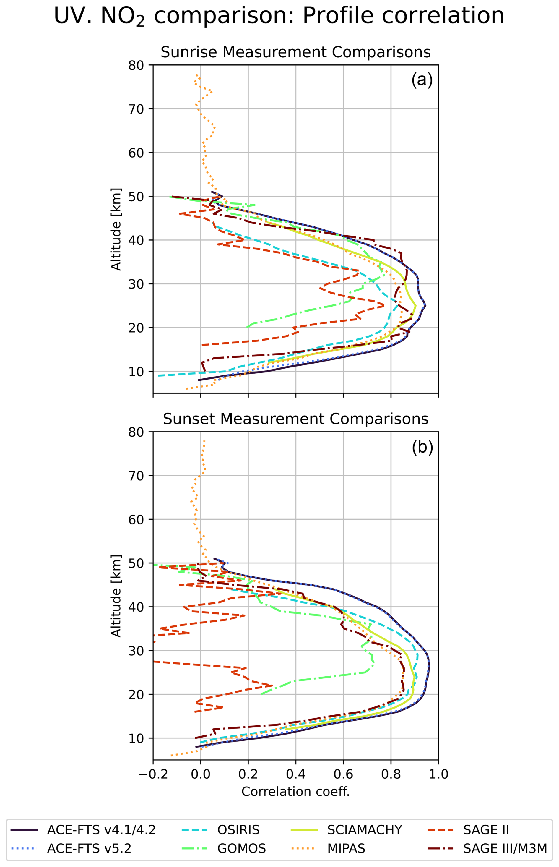
Figure 13 shows the correlation between MAESTRO and the comparison datasets. The vertical range with the best correlation for most datasets is approximately 15 to 40 km. Within this span, the highest correlation is found with the two versions of ACE-FTS, which have a sunrise (sunset) measurement correlation of at least 0.87 (0.89). Over this range, the OSIRIS sunset, SCIAMACHY, MIPAS, and SAGE III/M3M comparisons all have an average correlation above 0.75. The OSIRIS sunrise comparison is somewhat worse overall, with an average correlation of 0.65, and GOMOS also has lower correlation, at 0.60 (0.59) for the sunrise (sunset) comparison, due to the poor correlation found between it and MAESTRO between 20 and 25 km. Likely influenced by the few coincident profiles, as well as a systematic difference in sampling location, the SAGE II average sunrise correlation is only 0.49 for this range, and the sunset comparisons are found to be uncorrelated, with an average correlation coefficient of −0.03. However, despite this variable level of agreement, most datasets show generally moderate or good correlation over this range. Outside of this range, the correlation of most of the datasets quickly falls to below 0.50, with the majority of the datasets reaching this threshold between 11 and 13 km and between 41 and 43 km. The drop in correlation coefficients outside of the 15–40 km range, along with the calculated relative and absolute differences, indicates that the NO₂ product should primarily be used in the lower and middle stratosphere.

5 Conclusions

In this study, the recently released version 4.5 ozone and NO₂ retrieval products from MAESTRO have been compared against coincident measurements for validation purposes. A total of 12 datasets were used for these comparisons; however, only the Vis-ozone product from MAESTRO was assessed using all 12 datasets due to the limited viability of MAESTRO UV products, which span only from the start of the ACE mission until 2009, and the lack of an NO₂ product from two of the instruments employed.

Before addressing the individual products, it is crucial to note that, for all three MAESTRO products, the best agreement is generally found with ACE-FTS. This agreement is important due to the two instruments sharing a line of sight while also employing different measurement techniques and retrieval schemes. As the shared line of sight eliminates the majority of the influence of geophysical variability on the measurements compared, the differences between the two sets of products arise almost entirely from instrumental and retrieval technique differences. Thus, we can conclude that the two instruments are largely consistent and that both instruments likely have good retrieval techniques.

The Vis-ozone product was found to have excellent agreement with the coincident datasets, with average relative differences of between 2.3 % and 8.2 % from 20 to 50 km and high correlation coefficients, generally in excess of 0.71, between 15 and 40 km. The UV-ozone product from MAESTRO was found to agree slightly less well with the coincident datasets, with average relative differences between 20 and 45 km of 2.8 % to 11.9 %. From 15 to 35 km, good correlation was found between the UV-ozone product and the coincident datasets, with correlation coefficients typically in excess of 0.70 on average. Both datasets show a small high bias in the stratosphere, compared with the comparison instruments. Despite the good agreement found over the stratosphere, both MAESTRO ozone products have been found to show significant differences from the other datasets in the mesosphere. Analysis of the mean ozone profiles constructed from the MAESTRO ozone profiles, as well as the standard deviation thereof, indicated that the MAESTRO version 4.5 retrieval appears to over-constrain the ozone concentration in the mesosphere, resulting in the near-0 ppmv concentrations observed over this region, which show considerable disagreement with those from the other datasets. Thus, scientific applications of the MAESTRO ozone products should limit their use outside of the stratosphere.

Finally, UV NO₂ from MAESTRO was found to agree to within 27.2 % with the majority of the comparison datasets between 20 and 40 km, with the relative differences ranging from 8.5 % to 43.4 % on average over this span. A distinct low bias was identified for this product over the stratosphere. From 15 to 40 km, good correlation was found with most of the comparison datasets, with almost all of the comparison sets having average correlation coefficients over 0.70. The low bias observed over the stratosphere, coupled to a large concentration of NO₂ in the mesosphere, appears to be influenced by inaccurate partitioning of NO₂ in the MAESTRO version 4.5 retrieval, which seemingly results in the accumulation of NO₂ above 70 km in the profiles. When coupled to the limited range over which decent agreement is found with the comparison datasets, this indicates that the MAESTRO NO₂ product should only be used in the lower and middle stratosphere.

Overall, the findings presented in this work support the use of the MAESTRO version 4.5 dataset for stratospheric studies. The Vis-ozone product is viable from the start of the ACE mission (February 2004) through to the present, and the usage of this product should principally be confined to between 20 and 50 km. This Vis-ozone product is the preferred MAESTRO ozone product for general applications, due to the UV-ozone products only being viable until December 2009 and over a slightly narrower stratospheric range from 20 to 45 km; however, for studies focusing on UV-derived measurements of ozone, it is a valid dataset for consideration. Finally, the MAESTRO NO₂ product is found to only be viable from the start of the mission until June 2009, and general agreement with other datasets is only achieved between 20 and 40 km. As long as applications for this product are able to work within this limited range of viability, the MAESTRO NO₂ product should be suitable for scientific applications.