Forward model emulator for atmospheric radiative transfer using Gaussian processes and cross validation

Remote sensing of atmospheric carbon dioxide (CO₂) carried out by NASA's Orbiting Carbon Observatory-2 (OCO-2) satellite mission and the related uncertainty quantification effort involve repeated evaluations of a state-of-the-art atmospheric physics model. The retrieval, or solving an inverse problem, requires substantial computational resources. In this work, we propose and implement a statistical emulator to speed up the computations in the OCO-2 physics model. Our approach is based on Gaussian process (GP) regression, leveraging recent research on kernel flows and cross validation to efficiently learn the kernel function in the GP. We demonstrate our method by replicating the behavior of OCO-2 forward model within measurement error precision and further show that in simulated cases, our method reproduces the CO₂ retrieval performance of OCO-2 setup with computational time that is orders of magnitude faster. The underlying emulation problem is challenging because it is high-dimensional. It is related to operator learning in the sense that the function to be approximated maps high-dimensional vectors to high-dimensional vectors. Our proposed approach is not only fast but also highly accurate (its relative error is less than 1  %). In contrast with artificial neural network (ANN)-based methods, it is interpretable, and its efficiency is based on learning a kernel in an engineered and expressive family of kernels.

1 Introduction

Climate change, one of the most significant global environmental challenges, is primarily attributed to anthropogenic carbon emissions, which have accelerated the increase of carbon dioxide (CO₂) in the atmosphere, posing a threat to Earth's future. The industrial revolution marked the onset of increased CO₂ emissions due to the extensive use of fossil fuels in various industries, such as transportation, manufacturing, and agriculture. The Intergovernmental Panel on Climate Change underscores CO₂'s potent effect on planetary warming due to significant radiative forcing (IPCC, 2023). The atmospheric concentration of this trace gas is increasing at an ever faster rate, and as of May 2023, the measured CO₂ at Mauna Loa station was 424.0 ppm, a 3 ppm increase from a year before (421.0 ppm in May 2022). Although the global terrestrial biosphere and oceans each take up about 25 % of these emissions (Friedlingstein et al., 2022), this balance may not be sustainable, which might lead to unpredictable feedbacks in the carbon cycle and the global climate system. These couplings between the Earth's climate system and the carbon cycle can introduce significant uncertainty in future climate change projections (Friedlingstein et al., 2014), which further renders mitigation efforts increasingly challenging.

For reliable climate modeling and future scenario prediction, it is crucial to estimate carbon flux accurately (e.g., CarbonTracker, Peters et al., 2007), which involves quantifying both the sources and natural sinks of carbon. However, current in situ measurement networks are primarily deployed in the northern midlatitudes, leaving areas like the tropics underrepresented (Schimel et al., 2015). This lack of extensive coverage results in large uncertainties in flux estimates, underscoring the need for a more comprehensive global measurement network.

To provide a significant increase in coverage and resolution to the ground-based data set, global estimates of total column-averaged mole-fraction CO₂ (average amount of CO₂ over a vertical column of air at a specific ground pixel/location), denoted XCO₂, are collected using satellite-borne spectrometers. These instruments include the Japanese Greenhouse gases Observing SATellite (GOSAT, Kuze et al., 2009), operational since January 2009; the follow-on GOSAT-2 (Imasu et al., 2023) launched in October 2018; the Orbiting Carbon Observatory-2 from NASA (OCO-2, Crisp et al., 2012), launched in July 2014; the OCO-3 instrument (Eldering et al., 2019) taken to the International Space Station in May 2019; and the Chinese TanSat (Ran and Li, 2019) and TanSat 2 (Wu et al., 2023). Planned future missions include the Geostationary Carbon Cycle Observatory (GeoCarb, Moore et al., 2018), the European CO₂ Monitoring Mission (CO2M, Sierk et al., 2019), and the Global Observing Satellite for Greenhouse gases and Water cycle (GOSAT-GW, Kasahara et al., 2020). In this work, we focus exclusively on OCO-2, which, like all the abovementioned missions, measures solar radiance at the top of the atmosphere, reflected by Earth's surface and attenuated by atmospheric scattering and absorption by trace gases and aerosols. From these observed radiances, the OCO-2 mission uses a framework called optimal estimation (OE, Rodgers, 2004) to solve the related Bayesian inverse problem (see, e.g., Kaipio and Somersalo, 2005), referred to as a retrieval. OE is an iterative algorithm, returning an estimate of posterior mean and covariance as a Gaussian approximation to the nonlinear retrieval problem. Operationally, the retrieval problem is solved using the Atmospheric Carbon Observations from Space (ACOS) software (O'Dell et al., 2018), which implements OE using a state-of-the-art atmospheric full-physics (FP) model. Processing OCO-2 measurements with the ACOS algorithm is a computationally intensive task, and currently about one-third of prescreened clear soundings are used in a low-latency data processing stream (O'Dell et al., 2018). As the data record grows, computational speed is also a major hindrance for retrospective processing of the full collection of cloud-free soundings for the current and any future improved algorithms. Thus, computational efficiency is a limiting factor in releasing the improved data to the user community. These issues are certain to get even worse with upcoming wider-swath missions like CO2M and GOSAT-GW, as evidenced by another greenhouse gas imaging mission, Tropospheric Ozone Monitoring Instrument (TROPOMI, Veefkind et al., 2012), from regularly reprocessing their data record, which is more than 20 times greater in size than that of OCO-2.

As with all inverse problems, some approximations and assumptions have to be made in the ACOS algorithm. The resulting XCO₂ estimates have to be validated and bias-corrected using ground-based measurements from the Total Carbon Column Observing Network (TCCON, Wunch et al., 2017) and the COllaborative Carbon Column Observing Network (COCCON, Frey et al., 2019) as a reference. These sites are concentrated on the northern midlatitudes, and as a result of this coverage issue and the imperfections in the FP model, significant systematic errors persist in the data set. (See, e.g., Kiel et al., 2019, for the effect of systematic errors and Cressie, 2018, for an overview of statistical treatment of and issues in the retrieval.) Considerable effort has been exerted to tackle the high accuracy (less than 0.3 parts per million (ppm) in scenes with background levels of around 410 ppm) and high precision (standard errors less than 0.5 ppm) requirements of ingesting OCO-2 into flux inversion, which is the primary application of the data product (Gurney et al., 2002; Patra et al., 2007; Liu et al., 2017; Palmer et al., 2019; Crowell et al., 2019; Peiro et al., 2022; Byrne et al., 2023). Recent advancements in applying Markov chain Monte Carlo (MCMC, Brynjarsdóttir et al., 2018; Lamminpää et al., 2019) for non-Gaussian posterior characterization and simulation-based uncertainty quantification (Braverman et al., 2021) for capturing the overall uncertainty in the retrieval pipeline have been successfully deployed for addressing persisting retrieval errors. These methods, although comprehensive, suffer equally from computational speed issues as they require an extensive number of FP evaluations.

Computational speed issues in OE retrievals have been addressed in several ways. Neural network (NN)-based machine learning approaches (David et al., 2021; Mishra and Molinaro, 2021; Bréon et al., 2022) have been implemented to a combination of real-world radiance data and model atmospheres (outputs of computational atmospheric models, like the Copernicus Atmospheric Monitoring Services (CAMS) model; Chevallier et al., 2010). The OCO-2 forward model itself was sped up by using a surrogate model (Hobbs et al., 2017) that only partially considered the physical processes present in the FP model and more recently by using a Gaussian process (GP) emulator (Ma et al., 2019) for replicating the output of the FP model. In this paper, we will take a similar approach using GPs but with several improvements and an application to solving the retrieval problem with the help of closed-form Jacobians required in the gradient-based algorithm. GPs are a well-suited technique for forward model emulation, since they can be used with less data (130 K, David et al., 2021, for NN vs. 20 K for GP; see Sect. 4) and trained more quickly than NN-based approaches. Additionally, a GP provides uncertainty estimates and closed-form Jacobians trivially, which are not straightforward to extract from a NN. For training efficiency, our approach will leverage recent novel techniques for GP parameter learning called kernel flows (Owhadi and Yoo, 2019) and training data generation via evaluating the FP model using the Reusable Framework for Atmospheric Composition (ReFRACtor) (McDuffie et al., 2020). We will demonstrate the accuracy of forward model emulation against a holdout test set of FP evaluations and further demonstrate the ability of our emulator to replicate the OE retrieval performance of ReFRACtor FP model in a fraction of the computational time. Our approach achieves a remarkably low prediction error, less than 1 % (“within measurement error limits”), which is an excellent result in the field of more general operator learning. Strategies to achieve learning more complicated operators, like the FP model in our case, often involve a NN-based architecture (Lu et al., 2021; Li et al., 2024). Our approach follows the example set by Batlle et al. (2023) that kernel methods are competitive in operator learning.

The rest of the paper is organized as follows. Section 2 will describe in detail the GP regression, kernel learning, and the resulting forward model emulator. Section 3 will further elaborate on the details of the OCO-2 retrieval algorithm, the state vector, and the FP model describing atmospheric radiative transfer. Section 4 will detail the emulator implementation of the ReFRACtor FP model and assess its performance. Section 5 will show results of our emulator used in a simulated XCO₂ retrieval context, and finally Sect. 6 will provide concluding remarks and ideas on future work and applications.

2 Gaussian process emulator

Gaussian process (GP) regression (Rasmussen and Williams, 2006) (also called kriging in spatial context: Cressie, 1993; Stein, 1999) is a well-studied methodology for approximating any continuous function to an arbitrary accuracy, leveraging training data and a kernel function prescribed a priori. In addition, once trained, the GP model can be used to obtain fast and accurate predictions of a computationally demanding physics model, to estimate prediction uncertainty, and to compute closed-form derivatives and Jacobians for the prediction. Physical constraints like positive parameter values can be accounted for in training data design (which we address in later sections) so that predictions happen with the support of a training data set. This is to say that our training data set will cover the expected minimum and maximum values of each parameter in the state vector. For example, surface albedo is physically restricted between 0 (no reflected light) and 1 (full reflection). If our training data are sufficiently well spread covering this range, we can make good predictions essentially by interpolation with the physically feasible interval. Potential departure from this support can be detected by large prediction uncertainty values, as the prediction uncertainty of a GP gets large by design if the input location does not have training points near it. In this section, we outline the basic theory of GP regression and outline our approach to modeling the continuous function between atmospheric state vectors x and radiances y observed by the OCO-2 instrument. We also provide background on maximum likelihood estimation for fitting GP models and present a novel root mean square error (RMSE) cross-validation extension for the kernel flow (Owhadi and Yoo, 2019) approach, which we employ for the rest of this work.

2.1 Gaussian process regression

To construct an emulator for the forward model F(x), we employ Gaussian process (GP) regression to predict a label $z^{*}\in \mathbb{R}$ at a new state ${\mathit{x}}^{*}\in {\mathbb{R}}^m$. A GP is defined by a kernel function (defined explicitly later) $k(x,x^{\prime })$: $\mathcal{X}\times \mathcal{X}\to \mathbb{R}$, where in the cases studied in this work 𝒳=ℝ^m. We denote by Γ[X,X] the matrix of all kernel function evaluations over the training data $\mathbf{X}\in {\mathbb{R}}^{m\times N}$ of N points with the entries $\mathbf{\Gamma }[\mathbf{X},\mathbf{X}{]}_{i,j}=k({\mathit{x}}_i,{\mathit{x}}_j)$, where x_i and x_j are the ith and jth training data points, respectively. Furthermore, $\mathbf{\Gamma }[{\mathit{x}}^{*},\mathbf{X}]$ denotes the vector of kernel evaluations of state x^* against all training points X. Using the training data together with vector of corresponding labels z∈ℝ^N, a GP prediction of label (or function value) at a new state x^* is given by

$$\begin{array}{}\text{(1)}& z^{*}\equiv \text{GP}\left({\mathit{x}}^{*}\right)=\mathbf{\Gamma }[{\mathit{x}}^{*},\mathbf{X}]{\left(\mathbf{\Gamma }[\mathbf{X},\mathbf{X}]+\mathit{\sigma }\mathbb{I}\right)}^{-\mathrm{1}}\mathit{z},\end{array}$$

where we have assumed without loss of generality that the training data are centered, and thus the GP has a zero mean. We add that the term ${\left(\mathbf{\Gamma }[\mathbf{X},\mathbf{X}]+\mathit{\sigma }\mathbb{I}\right)}^{-\mathrm{1}}\mathit{z}$ does not depend on the new input state, so it can be precomputed. This makes the predictions take minimal computational time by avoiding inverting a potentially large matrix ${\left(\mathbf{\Gamma }[\mathbf{X},\mathbf{X}]+\mathit{\sigma }\mathbb{I}\right)}^{-\mathrm{1}}$.

In GP literature, the variance term σ𝕀 is usually taken to be the measurement error or local-scale unexplained variability in the training labels z. However, since we are interested in reproducing the outputs of a computer code, the “measurements” are exact, and hence there is no measurement error. It was shown in Owhadi and Yoo (2019) that learning the parameters of GP models from noiseless data can lead to unstable predictive models and numerical singularities. For this reason, we treat σ as a regularization parameter, which captures the empirical mismatch between the model and the actual data, and optimize it together with other kernel parameters.

In addition to point predictions, GP prediction can be associated with prediction uncertainty (the posterior variance of the GP), given by

$$\begin{array}{}\text{(2)}& {\mathit{\sigma }}^{*}=k({\mathit{x}}^{*},{\mathit{x}}^{*})-\mathbf{\Gamma }[{\mathit{x}}^{*},\mathbf{X}]{\left(\mathbf{\Gamma }[\mathbf{X},\mathbf{X}]+\mathit{\sigma }\mathbb{I}\right)}^{-\mathrm{1}}\mathbf{\Gamma }[{\mathit{x}}^{*},\mathbf{X}{]}^T.\end{array}$$

The ability to include prediction uncertainties sets GP regression apart from many modern NN-based machine learning methods, which only provide a point estimate as a prediction. Large prediction variance can be an indication of departure from the support of a training data set, indicating that GP is likely to lose its prediction skill. Additionally, uncertainty from the predictions can be propagated forward and accounted for in further applications of GP-based emulators.

The GP formulas presented here rely on conditional Gaussian distributions and thus have a similar structure to that of optimal interpolation (OI; e.g., p. 157 of Kalnay, 2002) and related iterative optimal estimation (OE) algorithms (e.g., Eq. 15), both of which are widely used methods in atmospheric remote sensing. OI and OE use Gaussian assumptions to derive a mean and covariance for the posterior distribution as a solution to an inverse problem, i.e., data assimilation or a retrieval. In Gaussian process regression, the target function (here, the forward model) is represented similarly by a Gaussian distribution that has a mean (prediction) and covariance (error estimate of the prediction).

Our interest will be in replicating the results of a gradient-based optimization problem. Hence, in addition to fast evaluations of F(x), we would also benefit from fast derivatives obtained from closed-form expressions. Combining Eqs. (1) and (4), we get

$$\begin{array}{}\text{(3)}& {\displaystyle \frac{\text{d}}{\text{d}{\mathit{x}}^{*}}}{z}^{*}={\displaystyle \frac{\text{d}}{\text{d}{\mathit{x}}^{*}}}\mathbf{\Gamma }\left[{\mathit{x}}^{*},\mathbf{X}\right]{\left(\mathbf{\Gamma }\left[\mathbf{X},\mathbf{X}\right]+\mathit{\sigma }\mathbb{I}\right)}^{-\mathrm{1}}\mathit{z},\end{array}$$

which describes taking the derivative of Eq. (1) with respect to x^*.

While other machine learning methods, such as artificial neural networks and multilayer perceptrons, can in principle be differentiated, computing the derivatives of a large architecture is computationally more demanding than evaluating Eq. (3), which motivates our use of GP regression. Other similar approaches (e.g., radial basis function networks) can be shown to be universal approximators as well and could be used in place of GPs. As will be shown, our approach yields a fast and accurate predictor that is intuitive and relatively easy to implement, so comparison against other machine learning methods will not be pursued further in the scope of this work.

2.2 Kernel function

A crucial modeling choice in GP regression is specification of a kernel function. This task involves either expert knowledge of the domain structure or some iterative trial-and-error search. In our application, we have empirically observed that a kernel function consisting of the sum of Matérn and linear kernels yields excellent predictive performance. This is likely due to a locally near-linear behavior commonly assumed with the OCO-2 forward model being captured by the linear kernel, together with a largely flexible Matérn term that is known to capture a large variety of nonlinear effects. The Matérn kernel is a more expressive choice of kernel compared to the usual Gaussian/radial basis functions used by default in Gaussian process regression, which tend to be “too smooth” to capture more abrupt changes in the function that is being approximated. Furthermore, such a kernel can also be differentiated in closed form. The kernel function used throughout this work is given by

$$\begin{array}{}\text{(4)}& \begin{array}{rl}k(\mathit{x},{\mathit{x}}^{\prime })& ={\mathit{\alpha }}_{\mathrm{1}}\left(\mathrm{1}+{\displaystyle \frac{\sqrt{\mathrm{3}}}{l}}\Vert (\mathit{x}-{\mathit{x}}^{\prime }){\Vert }_{\mathcal{W}}\right)\\ & \exp \left(-{\displaystyle \frac{\sqrt{\mathrm{3}}}{l}}\Vert (\mathit{x}-{\mathit{x}}^{\prime }){\Vert }_{\mathcal{W}}\right)+{\mathit{\alpha }}_{\mathrm{2}}\left(\mathcal{W}\mathit{x}{)}^T\right(\mathcal{W}{\mathit{x}}^{\prime }),\end{array}\end{array}$$

where $\Vert (\mathit{x}-{\mathit{x}}^{\prime }){\Vert }_{\mathcal{W}}=\sqrt{(\mathit{x}-{\mathit{x}}^{\prime }{)}^T{\mathcal{W}}^{\mathrm{2}}(\mathit{x}-{\mathit{x}}^{\prime })}$, 𝒲=diag(w) is a diagonal matrix, w∈ℝ^m is a vector of weights, l∈ℝ is a length scale parameter, and α₁ and ${\mathit{\alpha }}_{\mathrm{2}}\in {\mathbb{R}}_{+}$ are positive weights that are restricted to sum to 1.

To compute Jacobians, we need an expression for the derivative of the kernel function $\frac{\text{d}}{\text{d}{\mathit{x}}^{*}}\mathbf{\Gamma }[{\mathit{x}}^{*},\mathbf{X}]$ in Eq. (3). This can be computed in closed form from Eq. (4) using known matrix identities. The derivation of a closed-form expression can be found in Appendix A.

2.3 Parameter learning

Prediction quality of GP regression depends on identifying the hyperparameters θ that best fit the training data. In our case, following the form of our kernel function, we have $\mathit{\theta }=\left[\mathit{w},l,\mathit{\sigma },{\mathit{\alpha }}_{\mathrm{1}},{\mathit{\alpha }}_{\mathrm{2}}\right]$. Hyperparameters are commonly learned via optimization, using maximum likelihood estimation (MLE, Rasmussen and Williams, 2006). This amounts to minimizing

$$\begin{array}{}\text{(5)}& \mathcal{L}\left(\mathit{\theta }\right)=-{\displaystyle \frac{\mathrm{1}}{\mathrm{2}}}\log \left[\text{det}\left({\mathbf{\Gamma }}_{\mathit{\theta }}\right)\right]-{\displaystyle \frac{\mathrm{1}}{\mathrm{2}}}{\mathit{z}}^T\mathbf{\Gamma }(\mathit{\theta }{)}^{-\mathrm{1}}\mathit{z},\end{array}$$

where $\mathbf{\Gamma }\left(\mathit{\theta }\right)=\mathbf{\Gamma }[\mathbf{X},\mathbf{X}]$ evaluated at parameter values θ. Although this method is usually robust and performs well, GP applications with high-dimensional inputs and a large amount of training data are known to be challenging due to inverse matrix and log-determinant calculations. Numerous approaches have been suggested to tackle this problem (e.g., local approximations, Vecchia, 1988; Datta et al., 2016). Inspired by the kernel flow approach (Owhadi and Yoo, 2019) where kernel parameters are learned by minimizing a relative reproducing kernel Hilbert space (RKHS) norm, we propose a cross-validation RMSE-based method to be used in this work. Intuitively, RKHS norm is a way to measure the smoothness of a function approximation achieved with the kernel method. While smooth methods generally yield discretization-invariant predictors, we propose to directly minimize the prediction error instead. The intuition of this approach is to iteratively select small mini-batches of the training data set and individually leave points out one by one while using the rest of the mini-batch to predict the left-out values (via Eq. 1). Learning the kernel parameters that minimize this prediction error leads to globally good predictions given new inputs. This approach leverages the known screening effect associated with Matérn kernels, where the effects of faraway points on prediction accuracy diminish, and only close-by points are necessary for prediction accuracy. The same intuition is the basis of numerous nearest neighbors GP methods (e.g., Vecchia, 1988). The upside of our approach is the ability to select small mini-batches on each training iteration, allowing for faster computations while avoiding expensive log-determinant calculations and inverting the large covariance matrices required in MLE. We will later show that our proposed method converges reliably and yields excellent predictions.

We start by selecting a mini-batch X^batch and z^batch of size N_batch by randomly sampling from training data. We define a leave-one-out (LOO) cross-validation loss function with respect to L² error (also known as RMSE) by first considering taking out one data point from the training data and using the rest to predict it. This can be achieved by modifying the GP prediction formula from Eq. (1) and leaving out the ith data point. This is achieved via a rank-one downdate $\stackrel{\mathrm{̃}}{\mathbf{\Gamma }}(\mathit{\theta }{)}^{-\mathrm{1}}-\frac{\stackrel{\mathrm{̃}}{\mathbf{\Gamma }}\left(\mathit{\theta }{)}_{:,i}^{-\mathrm{1}}\stackrel{\mathrm{̃}}{\mathbf{\Gamma }}\right(\mathit{\theta }{)}_{:,i}^{-T}}{\stackrel{\mathrm{̃}}{\mathbf{\Gamma }}(\mathit{\theta }{)}_{i,i}^{-\mathrm{1}}}$ to remove the effect of the ith data point from the inverse covariance matrix $\stackrel{\mathrm{̃}}{\mathbf{\Gamma }}(\mathit{\theta }{)}^{-\mathrm{1}}$. (See Stewart, 1998, and Zhu et al., 2022, for details.) The modified LOO prediction formula is then given by

$$\begin{array}{}\text{(6)}& \stackrel{\mathrm{̃}}{\text{GP}}(\mathit{\theta },i)=\stackrel{\mathrm{̃}}{\mathbf{\Gamma }}(\mathit{\theta }{)}_{:,i}^T\left(\stackrel{\mathrm{̃}}{\mathbf{\Gamma }}(\mathit{\theta }{)}^{-\mathrm{1}}-{\displaystyle \frac{\stackrel{\mathrm{̃}}{\mathbf{\Gamma }}\left(\mathit{\theta }{)}_{:,i}^{-\mathrm{1}}\stackrel{\mathrm{̃}}{\mathbf{\Gamma }}\right(\mathit{\theta }{)}_{:,i}^{-T}}{\stackrel{\mathrm{̃}}{\mathbf{\Gamma }}(\mathit{\theta }{)}_{i,i}^{-\mathrm{1}}}}\right){\mathit{z}}^{\text{batch}},\end{array}$$

where $\stackrel{\mathrm{̃}}{\mathbf{\Gamma }}\left(\mathit{\theta }\right)=\mathbf{\Gamma }\left({\mathbf{X}}^{\text{batch}},{\mathbf{X}}^{\text{batch}}\right)$ is the N_batch×N_batch covariance over the mini-batch evaluated at parameter values θ, Here, the notation $\stackrel{\mathrm{̃}}{\mathbf{\Gamma }}(\mathit{\theta }{)}_{:,i}$ means all rows of the ith column. We then define the final loss function by using Eq. (6) to predict z_i (the ith training label removed from the mini-batch) as

$$\begin{array}{}\text{(7)}& \mathit{\rho }\left(\mathit{\theta }\right)=\sum _{i=k_{\mathrm{1}}}^{k_p}{\left(\stackrel{\mathrm{̃}}{\text{GP}}(\mathit{\theta },i)-z_i\right)}^{\mathrm{2}}+\mathit{ϵ}\Vert {\mathit{\theta }}_{\mathrm{0}}-\mathit{\theta }{\Vert }^k,\end{array}$$

where $i\in \left[k_{\mathrm{1}}\mathrm{\dots }{k}_p\right]\subset \left[\mathrm{1}\mathrm{\dots }{N}_{\text{batch}}\right]$ is a subset of p≤N_batch indices denoting elements of the mini-batch selected for prediction, which can be chosen as, for example, the entire mini-batch or the p nearest neighbors of the center point of the mini-batch. The regularization term, with error norm $\Vert \cdot {\Vert }^{\mathrm{2}}$, some penalty magnitude ϵ, and mean θ₀, is included to ensure that kernel amplitude parameter values do not grow uncontrollably. This is done since we have observed empirically that letting non-identifiable parameters grow during optimization can lead to the optimizer getting “stuck”, whereas this problem is not observed when regularizing the loss function. One may, for example, set θ₀ to be a vector of 1's.

We can now optimize the kernel parameters iteratively by repeatedly selecting mini-batches and updating θ along the gradient of ρ(θ), which is obtained by automatic differentiation using Julia's Zygote package (Innes, 2019). We note that closed-form kernel derivatives could be used here as well, but since automatic differentiation with mini-batch sizes we use uses negligible computational time, we will not pursue this idea further in this work. We note that as the mini-batch is selected at random, this method can be viewed as stochastic gradient descent. For this reason, we use the adaptive moment estimation (ADAM, Kingma and Ba, 2017) optimizer to find the optimal value. Use of a momentum-based optimizer is further recommended in this application as we have observed that the cost function often has several local minima. The optimization procedure is summarized in Algorithm 1. The final parameter value can be selected to be the one corresponding to the smallest loss function value achieved during training.

Algorithm 1 Kernel parameter learning

Input:

kernel function k, training data (X,z), batch size N_batch, number of prediction points p, number of iterations N_Iter.

Output:

matrix of kernel parameters Θ and vector of loss values R

1:

initialize ${\mathit{\theta }}_{\mathrm{1}}\leftarrow \mathrm{1},\mathrm{\Theta }\leftarrow \mathbf{0},\mathbf{R}\leftarrow \mathbf{0}$

2:

for all i in 1…N_Iter do

3:

${\mathbf{X}}^{\text{batch}}\leftarrow \mathbf{X}\left[\text{rand}\right(N_{\text{batch}}\left)\right],{\mathit{z}}^{\text{batch}}\leftarrow \mathit{z}\left[\text{rand}\right(N_{\text{batch}}\left)\right]$ // Randomly select a mini-batch X^batch,z^batch

4:

R[i]←ρ(θ_i) // Compute loss ρ(θ_i) from Eq. (7)

5:

$\mathbf{\Theta }\left[i\right]\leftarrow {\mathit{\theta }}_{i+\mathrm{1}},{\mathit{\theta }}_{i+\mathrm{1}}\leftarrow {\mathit{\theta }}_i+\text{ADAM}\left(\frac{\partial }{\partial \mathit{\theta }}\mathit{\rho }\right({\mathit{\theta }}_i\left)\right)$ // Compute gradient $\frac{\partial }{\partial \mathit{\theta }}\mathit{\rho }\left({\mathit{\theta }}_i\right)$ and update parameters θ_i using ADAM

6:

end for

7:

return  Θ,R

2.4 Training data generation

As we aim to reproduce the performance of a function represented as computer code, we take advantage of the freedom to use a space-filling design for x in ℝ^m for training data creation. We first span the unit cube [0,1]^m with a Sobol' sequence (Sobol, 1967; Press et al., 1992) of N points. In practice we employ Julia's Sobol.jl (Johnson, 2020) package for this step. Then, using information about the minimum and maximum physically feasible value of each input dimension, we scale the unit cube to span the whole state space. During research, we tested other methods like random sampling and Latin-hypercube-based methods, which turned out to leave “holes” in training data set, meaning non-constant predictive performance over the entire data set. Sobol' sequences, meanwhile, span the entire input space more evenly. Sobol' sequences are a space-filling design akin to Latin hypercubes, providing optimality (observed experimentally) in generation of training data. We further evaluate the computational model F(x) at each training point, obtaining states $\mathbf{X}\in {\mathbb{R}}^{N\times m}$ and model outputs $\mathbf{Y}\in {\mathbb{R}}^{N\times n}$.

3 The Orbiting Carbon Observatory-2

In this section, we describe OCO-2 and the related measurements, physics model, state vector, and retrieval algorithm. Further information on these topics can be found in, for example, Connor et al. (2008), O'Dell et al. (2012), Crisp et al. (2012), O'Dell et al. (2018), and in the Algorithm Theoretical Basis Document (ATBD) (Boesch et al., 2015).

3.1 The OCO-2 instrument

OCO-2 is a NASA-operated satellite mission dedicated to providing data products of global atmospheric carbon dioxide concentrations (Crisp et al., 2004). The satellite is pointed towards Earth as it measures solar light reflected by Earth's surface and atmosphere, recorded as radiances. The OCO-2 instrument itself is composed of three spectrometers that measure light reflected from Earth's surface in the infrared part of the spectrum in three separate wavelength bands. These bands are centered around 0.765, 1.61, and 2.06 µm and are called the O₂ A-band (O2), the weak CO₂ band (WCO2), and the strong CO₂ band (SCO2), respectively. Each observation consists of 1016 radiances on separate wavelengths from each band (for more information, see, e.g., Crisp et al., 2017; Rosenberg et al., 2017). These measurements are then used to infer a state vector containing information on atmospheric properties like CO₂ concentration on 20 pressure levels, surface pressure, temperature, and aerosol optical depth (AOD). The state vector also includes surface properties like albedo and solar-induced chlorophyll fluorescence (SIF). The primary scalar quantity of interest is the column-averaged CO₂ concentration (XCO₂).

3.2 Atmospheric radiative transfer

A key part to inferring XCO₂ from observed radiances is the construction of a computational atmospheric radiative transfer model which describes how solar radiation is propagated, reflected, and scattered by Earth's surface and atmosphere. Together with an instrument model, this computer code is known as the full-physics (FP) model, referred to in this work as

$$\begin{array}{}\text{(8)}& \mathit{y}=F(\mathit{x},\mathit{b}),\end{array}$$

where y is the output of the FP model (a wavelength-by-wavelength radiance), x is a state vector containing atmospheric and surface information, and b denotes model parameters held fixed during data processing. A thorough description of the FP model is given in the ATBD (Boesch et al., 2015). To motivate our emulation approach, we will here describe parts of the forward model physics, which is not intended to be a full description of the included physics. Rather, we leverage this information to better design our emulator.

Part of the radiance comes from absorption of radiation by atmospheric molecules, given by

$$\begin{array}{}\text{(9)}& I\left(\mathit{\lambda }\right)=f_{\mathrm{0}}\left(\mathit{\lambda }\right)\cos \left({\mathit{\tau }}_{\mathrm{0}}\right)\cdot R(\mathit{\lambda },\mathit{\theta },{\mathit{\theta }}_{\mathrm{0}},\mathit{\phi }-{\mathit{\phi }}_{\mathrm{0}})\exp \left(-g\left(\mathit{\lambda }\right)\right),\end{array}$$

where λ is wavelength, the jth wavelength corresponds to the jth entry of radiance y, f₀(λ) is the solar flux at the top of the atmosphere, $R(\mathit{\lambda },\mathit{\theta },{\mathit{\theta }}_{\mathrm{0}},\mathit{\phi }-{\mathit{\phi }}_{\mathrm{0}})$ is the reflectance of the surface, g(λ) is an integral over radiation path length that sums over for all modeled absorbers, θ and φ are the observation zenith and azimuth angles, and θ₀ and φ₀ are the corresponding solar zenith and azimuth angles. Observation and solar angles have a significant effect on the observed and modeled radiances, which will be important later in this work.

After calculating the absorption with Eq. (9), equations further describing atmospheric scattering are employed to solve for atmospheric radiative transfer (RT), which describes the total effect of atmosphere and surface on the scattered photons. The FP framework further includes an instrument model, which describes the effects of the observing system to the top-of-the-atmosphere radiances. These effects include instrument Doppler shift, spectral dispersion, and convolution with the instrument line shape (ILS) function, reducing the resolution from the finer RT grid to the coarser observational grid. On an abstracted level, this corresponds mathematically to

$$\begin{array}{}\text{(10)}& I_{\text{OBS}}\left(\mathit{\lambda }\right)=C_{\mathrm{1}}\left(\mathit{\lambda }\right)\underset{-\mathrm{\infty }}{\overset{+\mathrm{\infty }}{\int }}\text{RT}\left({\mathit{\lambda }}^{\prime }\right)\text{ILS}(\mathit{\lambda },{\mathit{\lambda }}^{\prime })\text{d}{\mathit{\lambda }}^{\prime }+C_{\mathrm{2}}\left(\mathit{\lambda }\right),\end{array}$$

where C₁(λ) and C₂(λ) denote the instrument effects other than convolution that can be expressed as multiplication and addition. Generally speaking, the instrument effects depend on different physical properties that can vary between detector arrays, while the RT portion of the forward model is constant within the instrument. This observation motivates us to focus on emulating the outputs of the RT, referred to as monochromatic radiances, after which instrument functions can be applied appropriately after the fact. Looking forward to operational integration of our emulator, this will reduce the complexity of the emulated system and arguably make our task easier.

3.3 OCO-2 state vector

The state vector elements comprising x for the FP model are summarized in Table 1. Notably, we have divided the table into two parts. The upper half lists the previously mentioned atmospheric and surface state vector elements that affect the RT part only, and the rest having to do with the instrument effects are in the lower half. This collection includes scaling factors for empirical orthogonal functions (EOFs) that capture unmodeled offsets in the observed radiances (O'Dell et al., 2018).

Table 1 Elements of the OCO-2 state vector by functional group. The second column indicates the total elements per group. The check marks in the remaining columns indicate which wavelength bands are sensitive to changes in each variable.

In addition to state vector elements, the FP model is parameterized by a set of parameters that are held fixed based on auxiliary information, such as laboratory measurements or meteorological data sets. These parameters include instrument calibration details, spectroscopy properties for absorbing gases, land elevation, and aerosol microphysical parameters. These aerosol parameters arise from the selection of two dominant aerosol types as a function of space and time. All aerosol types have different optical properties. This choice is determined a priori by global maps based on meteorological knowledge and measurements (see Fig. 1). The possible dominant aerosol types are dust (DU), sulfate (SO), sea salt (SS), organic carbon (OC), and black carbon (BC). While constructing the emulator, we will consider data sets with a fixed pair of dominant aerosol species in order to decouple their physical effects from the rest of state vector. Separate emulators can then be constructed for each pair of aerosol species, and a selection of which one to use can be done by matching the measurement location with the appropriate types.

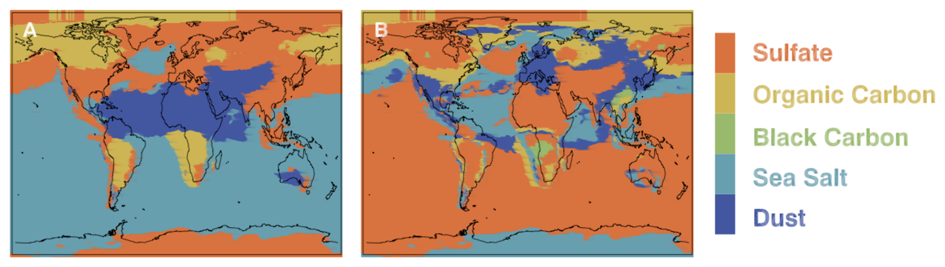
Figure 1 Example global map of (a) primary and (b) secondary aerosol types used in the OCO-2 FP model. Different aerosol types imply different physics, which needs to be taken into account when building a forward model emulator. Image taken from Boesch et al. (2015).

3.4 ReFRACtor

This work develops a proof-of-concept version of OCO-2 forward model emulator for a simulated case. For this reason and ease of access, we implement our simulations using the Reusable Framework for Atmospheric Composition (ReFRACtor, McDuffie et al., 2020). ReFRACtor is an extensible multi-instrument atmospheric composition retrieval framework that supports and facilitates combined use of radiance measurements from different instruments in the ultraviolet, visible, near-infrared, and thermal-infrared. It has been open-source since 2014 when it was first developed as the Level-2 processing code for OCO-2. Since 2017 the development team has worked to create a more general framework that supports more instruments and spectral regions. This framework has been developed to provide the broader Earth science community a freely licensed software package that uses robust software engineering practices with well-tested, community-accepted algorithms and techniques. ReFRACtor is geared not only towards the creation of end-to-end production science data systems, but also towards scientists who need a software package to help investigate specific Earth science atmospheric composition questions. Although ReFRACtor includes an implementation of a version of the OCO-2 production algorithm, the two have drifted since the initial intercomparison work was done. At that time it was validated against the B9.2.00 version of the software. For the most part mainly bug fixes have been kept in sync between the two versions. Additionally the core radiative transfer algorithms are the same, which justifies the use of ReFRACtor for constructing our emulator at this stage. Some minor additional algorithmic features made their way into the ReFRACtor version of OCO-2 from the production version. For the most part the major discrepancy will be due to changes in configuration values not implemented in ReFRACtor. These include values such as a priori and covariance versions, EOF data sets, ABSCO versions, and the solar model.

3.5 Retrieval algorithm

Inferring XCO₂ from measured radiances is an ill-posed inverse problem, which is referred to as performing a retrieval. The relationship between measurement and state is first modeled as

$$\begin{array}{}\text{(11)}& \mathit{y}=F\left(\mathit{x}\right)+\mathit{\epsilon },\end{array}$$

where data y∈ℝⁿ are a radiance vector; unknown x∈ℝ^m is the state vector, F; ℝ^m→ℝⁿ is the OCO-2 FP model; and ε∈ℝⁿ is the measurement uncertainty. For completeness, we summarize the operational retrieval algorithm used in OCO-2 processing. The retrieval proceeds with solving the inverse problem by using Bayesian formulation, in which the additive error ε and the prior for x are assumed to be Gaussian such that

$$\begin{array}{}\text{(12)}& \mathit{\epsilon }\sim \mathcal{N}\left(\mathrm{0},{\mathbf{S}}_{\mathit{\epsilon }}\right),\mathit{x}\sim \mathcal{N}\left({\mathit{x}}_{\mathit{a}},{\mathbf{S}}_{\mathbf{a}}\right).\end{array}$$

The measurement error covariance matrix S_ε is assumed to be diagonal, with elements for each wavelength j given by

$$\begin{array}{}\text{(13)}& {\mathit{\sigma }}_j^{\mathrm{2}}=k_{\mathrm{1}}{y}_j+k_{\mathrm{2}},\end{array}$$

where k₁ and k₂ are calibration parameters adjusted by the instrument calibration team. The a priori covariance is taken to be diagonal for non-CO₂ parameters, and the CO₂ profile is assumed to have a correlation structure shown in Fig. 2, which promotes continuous concentration profiles and limits the variability higher up in the atmosphere.

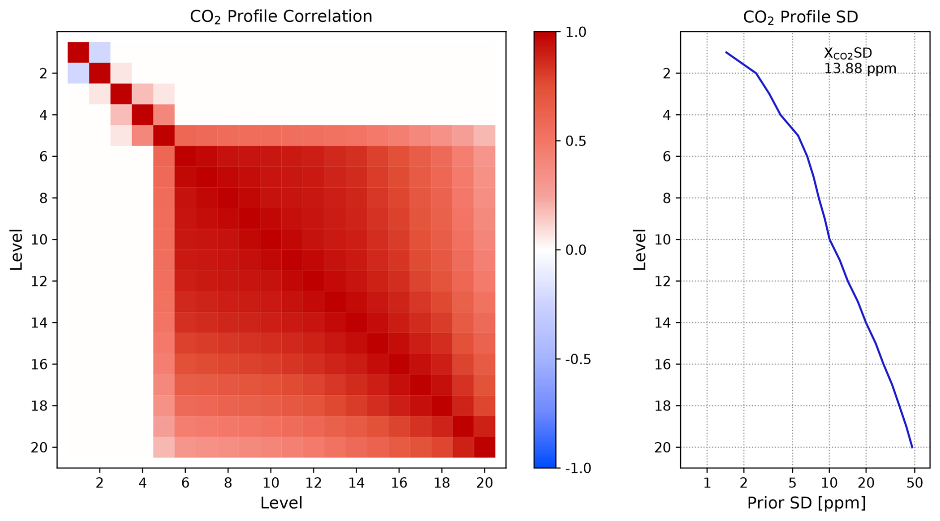
Figure 2 The a priori correlation matrix and standard deviation used for the CO₂ vertical profile in the OCO-2 retrieval. Vertical levels are ordered from the top of the atmosphere (Level 1) to the surface (Level 20).

The retrieval is operationally carried out using iterative gradient-based methods to solve for the maximum a posteriori estimate, which is equivalent to minimizing the cost function:

$$\begin{array}{}\text{(14)}& \begin{array}{rl}\widehat{\mathit{x}}& =\underset{\mathit{x}}{\text{argmin}}{\left(\mathit{y}-F\left(\mathit{x}\right)\right)}^T{\mathbf{S}}_{\mathit{\epsilon }}^{-\mathrm{1}}\left(\mathit{y}-F\left(\mathit{x}\right)\right)\\ & +\left(\mathit{x}-{\mathit{x}}_{\mathit{a}}\right){{\mathbf{S}}_{\mathbf{a}}}^{-\mathrm{1}}\left(\mathit{x}-{\mathit{x}}_{\mathit{a}}\right).\end{array}\end{array}$$

This optimization problem is solved using the Levenberg–Marquardt algorithm, in which at iteration i the state is updated according to

$$\begin{array}{}\text{(15)}& \begin{array}{rl}& \left((\mathrm{1}+\mathit{\gamma }){{\mathbf{S}}_{\mathbf{a}}}^{-\mathrm{1}}+{\mathbf{K}}_i^T{{\mathbf{S}}_{\mathit{\epsilon }}}^{-\mathrm{1}}{\mathbf{K}}_i\right)\text{d}{x}_{i+\mathrm{1}}\\ & =\left[{\mathbf{K}}_i^T{{\mathbf{S}}_{\mathit{\epsilon }}}^{-\mathrm{1}}\left(\mathit{y}-F\left({\mathit{x}}_i\right)\right)+{{\mathbf{S}}_{\mathbf{a}}}^{-\mathrm{1}}\left({\mathit{x}}_{\mathit{a}}-{\mathit{x}}_i\right)\right],\end{array}\end{array}$$

where γ is a damping parameter and K_i is the Jacobian of F(x) at iteration i. After each iteration, before updating the state, the effect of forward model nonlinearity is assessed by computing the quantity

$$\begin{array}{}\text{(16)}& R={\displaystyle \frac{c_i-c_{i+\mathrm{1}}}{c_i-c_{\text{FC}}}},\end{array}$$

where c_i is the value of the cost function (14) at iteration i, c_i+1 is similarly at iteration i+1, and c_FC is the cost function value assuming that $F({\mathit{x}}_i+\text{d}{\mathit{x}}_{i+\mathrm{1}})=F\left({\mathit{x}}_i\right)+{\mathbf{K}}_i\text{d}{\mathit{x}}_{i+\mathrm{1}}$ (i.e., a linear update). Based on the value of R, one of the following is executed:

• R ≤ 0.0001: γ is increased by a factor of 10. State is not updated.

• 0.0001 < R < 0.25: γ is increased by a factor of 10; ${\mathit{x}}_{i+\mathrm{1}}={\mathit{x}}_i+\text{d}{\mathit{x}}_{i+\mathrm{1}}$.

• 0.25 < R < 0.75: ${\mathit{x}}_{i+\mathrm{1}}={\mathit{x}}_i+\text{d}{\mathit{x}}_{i+\mathrm{1}}$.

• R > 0.75: γ is decreased by a factor of 2, ${\mathit{x}}_{i+\mathrm{1}}={\mathit{x}}_i+\text{d}{\mathit{x}}_{i+\mathrm{1}}$.

After each nondivergent step, convergence is assessed by computing the error variance derivative (see Boesch et al., 2015, for details). The operational retrieval further provides an estimate for the posterior covariance as a Laplace approximation:

$$\begin{array}{}\text{(17)}& \widehat{\mathbf{S}}={\left({\mathbf{K}}^T{\mathbf{S}}_{\mathit{\epsilon }}^{-\mathrm{1}}\mathbf{K}+{{\mathbf{S}}_{\mathbf{a}}}^{-\mathrm{1}}\right)}^{-\mathrm{1}}.\end{array}$$

This is done together with the so-called averaging kernel:

$$\begin{array}{}\text{(18)}& \mathbf{A}=({{\mathbf{S}}_{\mathbf{a}}}^{-\mathrm{1}}+{\mathbf{K}}^T{\mathbf{S}}_{\mathit{\epsilon }}^{-\mathrm{1}}\mathbf{K}{)}^{-\mathrm{1}}{\mathbf{K}}^T{\mathbf{S}}_{\mathit{\epsilon }}^{-\mathrm{1}}\mathbf{K},\end{array}$$

which can be interpreted as the sensitivity of the retrieved state $\widehat{\mathit{x}}$ to the true atmospheric state x. These quantities are important for downstream users of OCO data products, which highlights the value of producing closed-form Jacobians during data processing.

4 Forward model emulation

In this section, we will describe the practical implementation of our method laid out in Sect. 2 applied to the OCO-2 retrieval problem in Sect. 3. This includes data transformations and dimension reduction, training data generation, convergence of the optimizer in kernel parameter learning, and assessment of forward model output quality. We stress that in order to be implemented in an operational retrieval algorithm, the emulator is required to perform with superior accuracy. We ensure accurate performance by making sure that the error in predicted radiances, compared to FP outputs, is less than the radiance measurement error standard deviation. This way, any systematic errors in emulation will be masked by measurement noise, and retrieval performance using emulation will closely resemble that of using the FP model.

4.1 Data transformations

As GPs tend to perform worse with increasing input dimension and because the standard GP formulation is developed for one-dimensional outputs, we will need to reduce the dimension of both the atmospheric state and the radiance. For the atmospheric state x, we leverage the fact that OCO-2 measurements are made at three separate wavelength bands, which leads to the state vector having band-specific elements, which can be ignored when dealing with other bands. This partition has been summarized in Table 1. Earlier work by Ma et al. (2019) considered cross-band correlations while emulating OCO-2 radiances, but the authors finally showed that the bands are distant enough from one another in wavelength space that they can be treated independently. With this insight, we proceed by constructing separate GPs for each band and using only the sensitive dimensions of x as inputs. We further notice that the 20-element CO₂ profile is continuous and can be expressed as loadings obtained using principal component analysis (PCA). The most straightforward way to do this is by truncated singular value decomposition (SVD) of the empirical covariance matrix of state vectors (Tukiainen et al., 2016). To accomplish this, we use a simulation distribution derived by Braverman et al. (2021) for one selected set of realistic geophysical conditions as a basis for our experiments and perform SVD on the covariance matrix of this distribution. Analysis of singular value decay suggests that the CO₂ profile can be represented with just four principal components, which we collect to a matrix P_x as the four leading singular vectors. We then project the CO₂ profile to a principal component space and further standardize the states by using the mean and variance of the simulation distribution, leading to

$$\begin{array}{}\text{(19)}& \stackrel{\mathrm{̃}}{\mathit{x}}={\displaystyle \frac{\mathrm{1}}{{\mathit{\sigma }}_x}}\left(\text{diag}({\mathbf{P}}_x^T,{\mathbb{I}}_c)\left(\mathit{x}-\left[{\mathit{\mu }}_p,{\mathbf{0}}_c\right]\right)-{\mathit{\mu }}_x\right),\end{array}$$

where μ_p is the CO₂ profile mean, μ_x and σ_x are the state mean and state standard deviation, diag(A,B) denotes a block diagonal matrix with blocks A and B, 𝕀_c is a $c=m-\mathrm{16}$-dimensional identity matrix (as the profile is represented by 4 dimensions instead of original 20), and [μ_p,0_c] is a stacked vector of CO₂ profile mean and a c-dimensional zero vector.

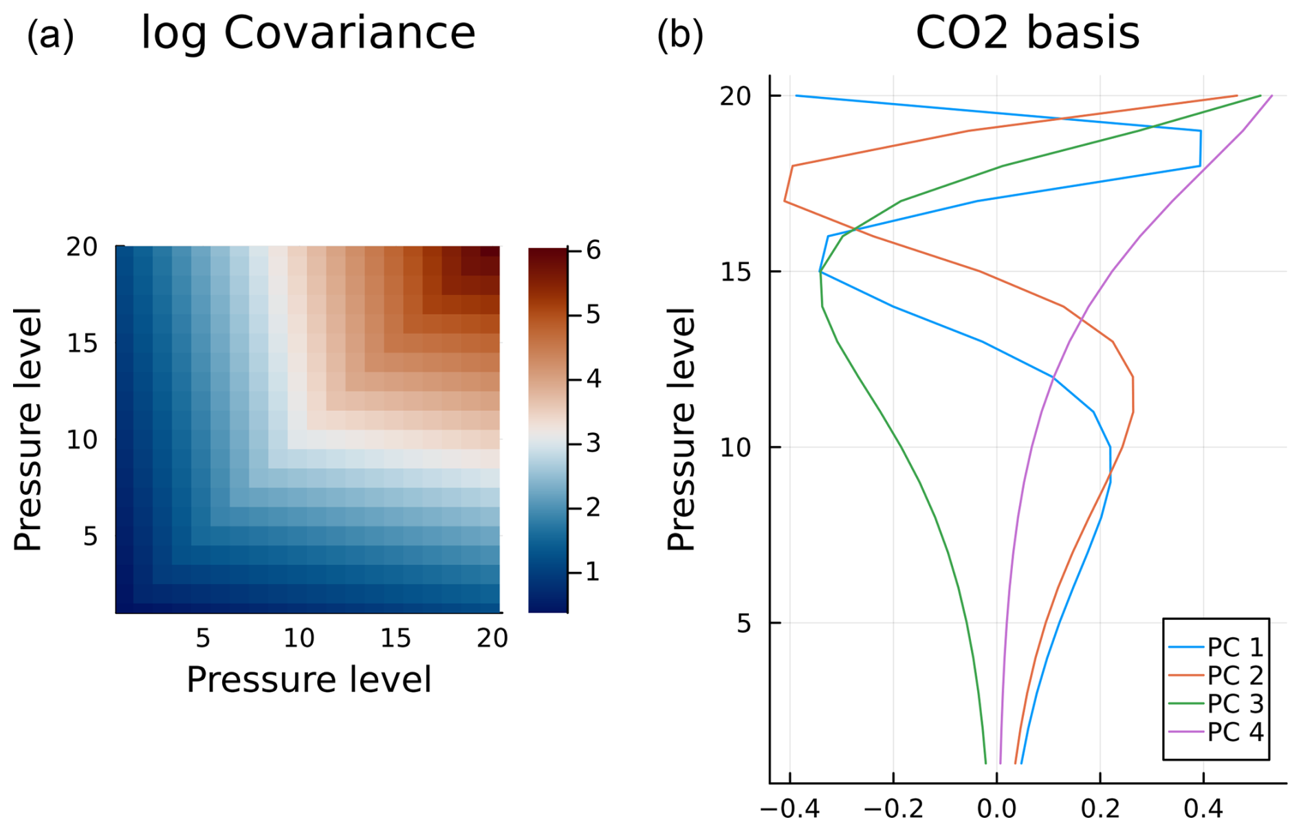
Figure 3 (a) The CO₂ profile covariance matrix of the simulation distribution used in this work. (b) Four leading singular vectors from the SVD of the covariance matrix.

Next, we generate training data using a Sobol' sequence (see Sect. 2.4). For this study, we can omit dispersion, EOF and SIF parts of the state vector (see Table 1), and fix them to the prior mean. This follows from the discussion in Sect. 3 focusing on monochromatic radiances. Omitting dispersion simplifies computations as the wavelength grid would otherwise shift, making SVD for radiance dimension reduction hard. Ma et al. (2019) solved this problem by employing functional principal component analysis, while we can proceed with ordinary SVD. The empirical orthogonal functions (EOFs) are included in the operational retrieval to reduce fit residuals and therefore make convergence analysis easier. These have no direct impact on our study and can be safely omitted. Furthermore, the SIF parameters are fit on the O2 band only as part of the instrument effects, and we do not include them in the emulation for this reason. As is evident from Eq. (9), the measurement geometry has a significant impact on the output of the FP model. For this reason we include three extra parameters, θ, θ₀, and φ−φ₀, to our training data vector. Sufficient and realistic limits to these parameters are obtained from the simulation distribution of Braverman et al. (2021) by considering a 4σ interval around the mean values. In all, we now have $m=\mathrm{4}+\mathrm{21}+\mathrm{3}=\mathrm{28}$ for input space, coming from profile PCs, other included state vector elements, and geometry. We create a Sobol' sequence of 20 000 points for training and scale all dimensions of the hypercube to $[-\mathrm{4},\mathrm{4}]$, corresponding to 4 standard deviations on the normalized $\stackrel{\mathrm{̃}}{\mathit{x}}$ basis. We further obtain the training data set in original space by reversing the transformation (19).

Training data Y (radiances) are obtained by evaluating the FP model on each x from the scaled Sobol' sequence. For this work, we choose a single realistic land nadir measurement to represent physical parameters not included in state vector x. We perturb sampling geometry to reflect relevant solar and instrument angles. For a real-world application this approach can be extended to include different scenes and other location-dependent parameters. To obtain the labels z, we similarly perform truncated SVD on the radiances Y separately on each wavelength band $B\in [\text{O2},\text{WCO2},\text{SCO2}]$ and collect the leading n_B singular vectors in matrices P_B. The four leading singular vectors for each band are included in Fig. 4 to present the kinds of features the most significant principal components, or basis vectors, encode. While this decomposition could hold additional information on physical processes behind the radiative transfer model, we do not pursue such an analysis further in this work. With additional standardization of the variables, we obtain the following transformations for each wavelength band B:

$$\begin{array}{}\text{(20)}& \stackrel{\mathrm{̃}}{{\mathit{z}}_B}={\displaystyle \frac{\mathrm{1}}{{\mathit{\sigma }}_z}}\left({\mathbf{P}}_B^T\left({\mathit{y}}_B-{\mathit{\mu }}_B\right)-{\mathit{\mu }}_z\right),\end{array}$$

where μ_B is the radiance mean, and μ_z and σ_z are the principal component mean and standard deviation for band B.

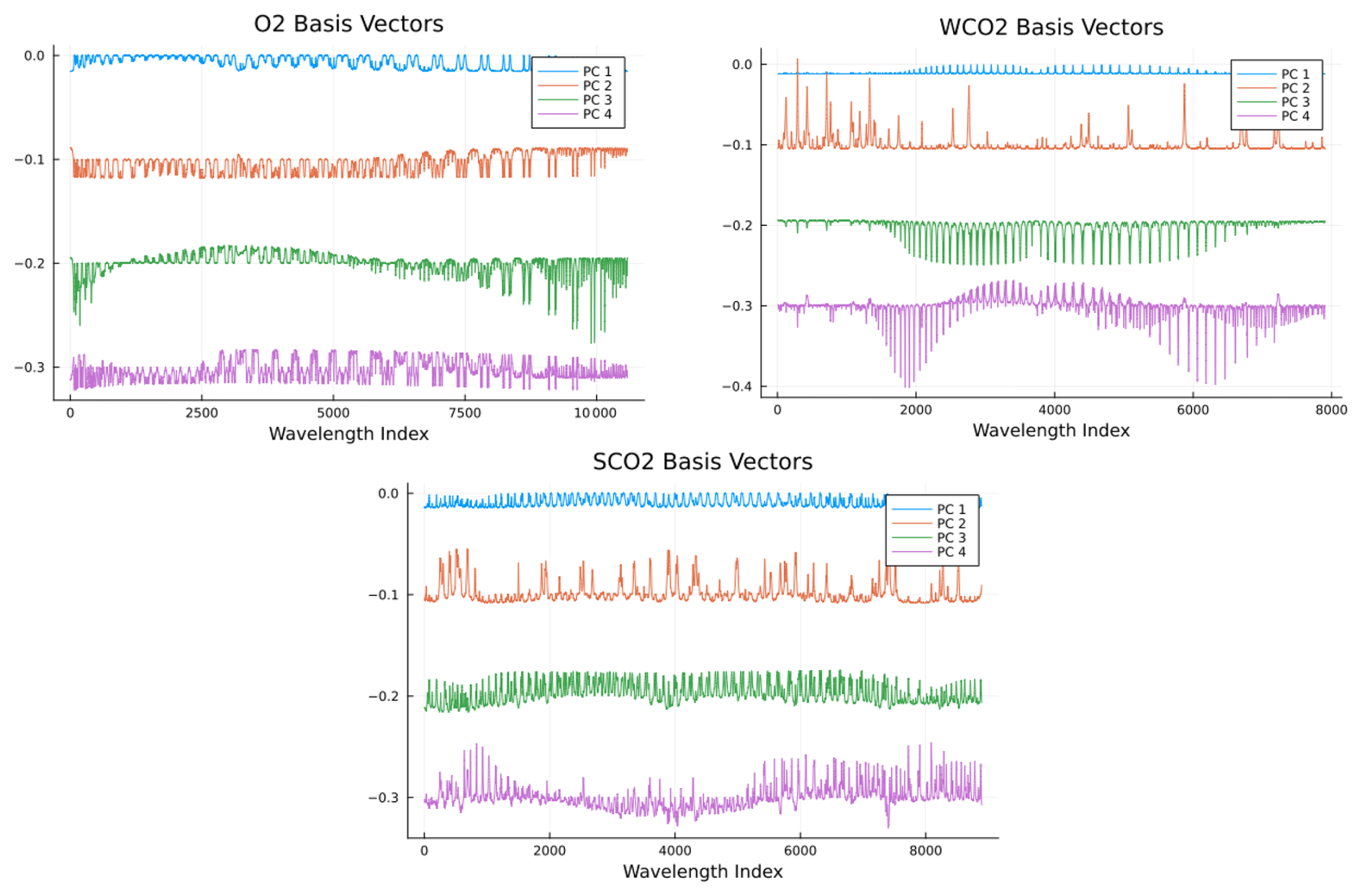
Figure 4 Leading four basis vectors obtained from the SVD (principal components, PCs) for radiances y for each band: O2, weak CO₂ (WCO2), and strong CO₂ (SCO2). Basis vectors 2–4 are offset for illustration purposes.

The quality of this approximation is assessed by plotting the reconstruction ${\mathbf{P}}_B{\mathbf{P}}_B^T({\mathit{y}}_B-{\mathit{\mu }}_B)+{\mathit{\mu }}_B$ over a holdout data set not used in computing the SVD. We illustrate in the upper panel of Fig. 5 the distribution of relative reconstruction error from this data set. We have further applied the instrument function to each residual and further divided them by the measurement error standard deviation given by Eq. (13). This metric is justified by the rationale that if the reconstruction error is less than or comparable to measurement error on the radiances, no significant amount of information is lost.

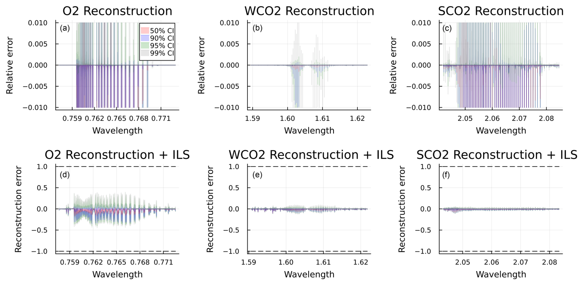
Figure 5 (a, b, c) Distribution of relative reconstruction error for monochromatic radiances on the O2, WCO2, and SCO2 bands. (d, e, f) Distribution of reconstruction error for all bands after applying the instrument function and dividing by measurement error standard deviation. Shading represents 50 % (red), 90 % (blue), 95 % (green), and 99 % (gray) confidence intervals.

The final emulator g(x) can now be summarized in Fig. 6, where ${\text{GP}}_i\left({\stackrel{\mathrm{̃}}{x}}_B\right)$ is the GP prediction given by Eq. (1), and the indices i, j, and k run through the number of principal components included in a given band. The effect of this choice will be examined further later in this work. The state is first normalized according to Eq. (19) for each band B, after which the GP-predicted principal component loadings are assembled back to radiances using relation in Eq. (20). When evaluating the emulator, each index is independent and can then be computed in parallel.

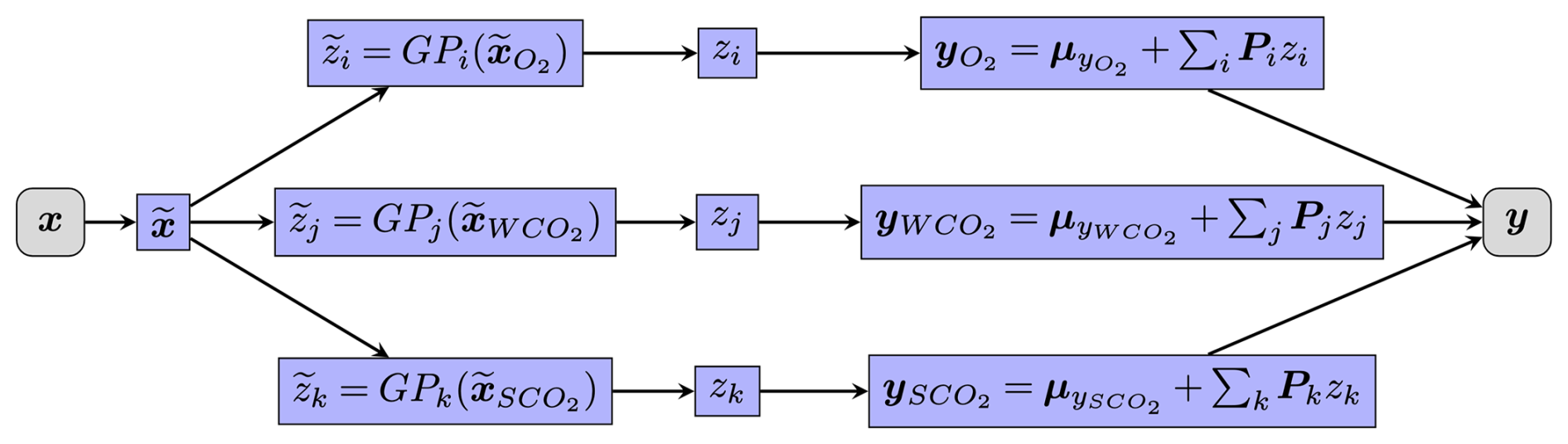
Figure 6 Diagram showing the step-by-step process of emulator evaluation. Transformation $\stackrel{\mathrm{̃}}{\mathit{x}}$ refers to normalization in Eq. (19); similarly $\stackrel{\mathrm{̃}}{\mathit{z}}$ denotes the scaling given in Eq. (20). $\text{GP}\left(\stackrel{\mathrm{̃}}{\mathit{x}}\right)$ denotes the GP prediction given by Eq. (1) of labels z, which are assembled back to radiances based on Eq. (20) for each band and each principal component i, j, and k therein.

4.2 Training

Having obtained training data $\stackrel{\mathrm{̃}}{\mathbf{X}}$ and z, we can now proceed in optimizing the kernel parameters as described in Sect. 2.3. We prescribe an individual GP per output parameter z_i. We have N = 20 000 for training data size, and we set M = 100 for mini-batch size, set p = 5 for the number of prediction points per mini-batch, and run the ADAM optimizer for 5000 iterations with a small learning rate – in our case 0.02. We initialize all other parameters at 1, except for linear component weight at 0 and the nugget at $\mathrm{1}\times {\mathrm{10}}^{-\mathrm{6}}$ for $\stackrel{\mathrm{̃}}{\mathit{x}}$. As outlined in Sect. 3.3, we further reduce the dimension of the input space by selecting only the indices that a given wavelength band is sensitive to, given by Table 1.

For testing the performance of the algorithm, we draw a random sample X^test from the same simulation distribution from Braverman et al. (2021) as independent test data, which is then used to evaluate the FP model to create radiances Y^test. For test data, we fix dispersion, EOFs, and SIF at prior values as before. Example behavior of the loss function together with evolution of the kernel parameter values and true vs. predicted z values is shown in Fig. 7. We see that during training, the loss function values converge to a small value close to 0. The fluctuations of loss function values are due to the ADAM optimizer effectively being a stochastic gradient descent method: each mini-batch is sampled randomly, which causes consequent steps, possibly resulting in higher values, while the running average still always decreases. We can also see the evolution of different kernel parameters: the weight of the linear component, for example, was initially set very close to 0. During training, the algorithm correctly identifies the significance of the linear term, and the relative importance of this term overtakes the nugget (corresponding to random noise). Resulting predictions of principal component loadings can be seen to land very tightly on the one-to-one line, indicating good performance over the whole test data. The distribution of true vs. predicted z values for each component on each wavelength band is further illustrated in Fig. 8. We conclude that the predicted values correspond the true values most of the time. Some principal components show a larger spread on prediction errors (e.g., O2 PC 9 or WCO2 PC 9). These principal components can be redundant and do not contain meaningful information about the radiance, since the total predictive performance still remains very accurate.

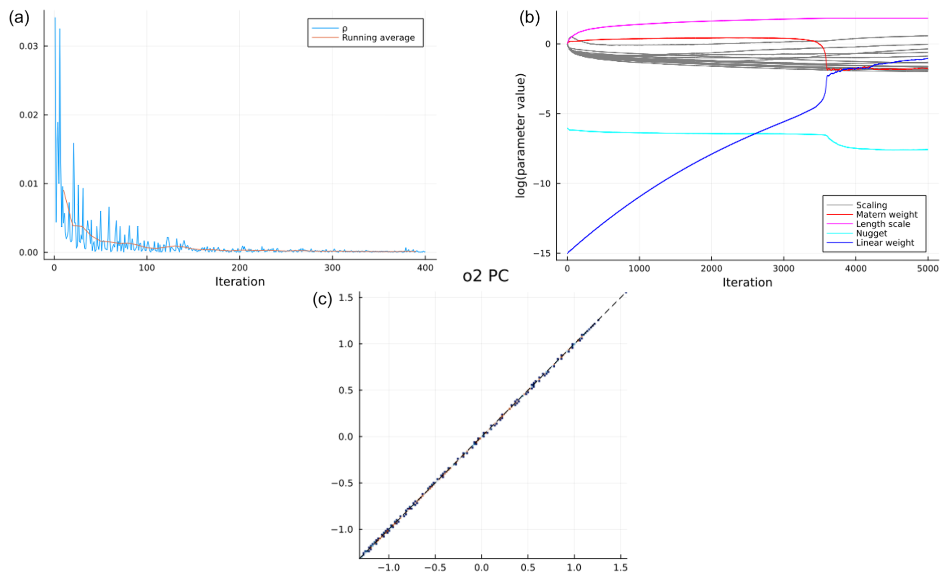
Figure 7 Example training performance for the first principal component of the O₂ band. (a) Loss function values for the first 400 iterations of parameter learning. The blue line depicts the cost function value per iteration. The red line depicts a cumulative running average of the cost function. (b) Evolution of the kernel parameters as a function of iteration. (c) True vs. predicted z values over a withheld test set for the first component of the O₂ band.

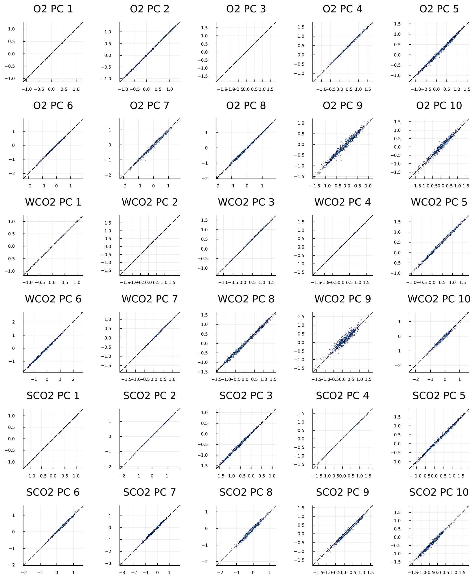
Figure 8 True versus predicted values for 10 radiance principal components on each wavelength band.

4.3 Predictive performance

Finally, we assemble the predicted z values back to radiances and compute the relative differences with the test data, shown in the upper panel of Fig. 9. On the lower panels, as before, we apply the instrument function to these residuals and divide by the measurement error standard deviation to underline that the desired performance would be to make less prediction error than measurement error.

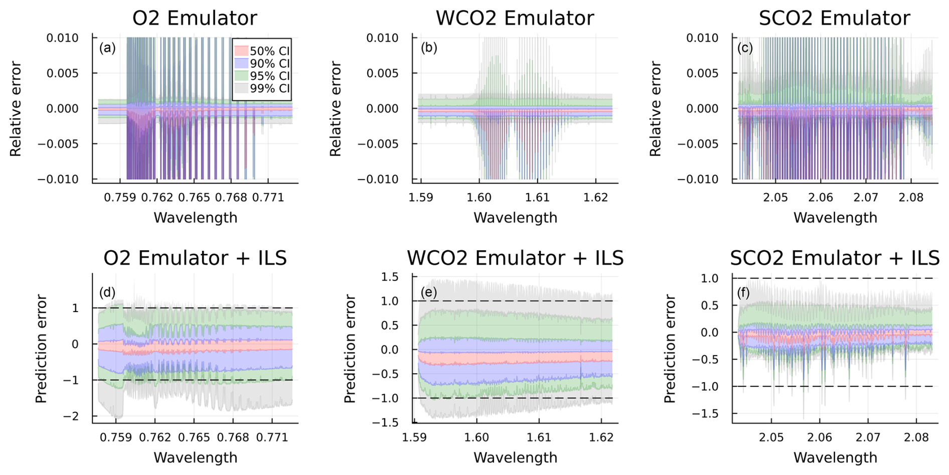
Figure 9 (a, b, c) Distribution of relative prediction error for monochromatic radiances on the O2, WCO2, and SCO2 bands. (d, e, f) Distribution of the prediction error for all bands after applying the instrument function and dividing by the measurement error standard deviation. Shading represents 50 % (red), 90 % (blue), 95 % (green), and 99 % (gray) confidence intervals.

After constructing the emulator obtaining radiances as outputs, we can further apply Eq. (3) to compute the Jacobians $\frac{\text{d}}{\text{d}\stackrel{\mathrm{̃}}{\mathit{x}}}\mathit{z}$. We can then reverse the normalizing transformations on both $\stackrel{\mathrm{̃}}{\mathit{x}}$ and y and further apply the instrument functions to our Jacobians to get back to the operational observation units. The Jacobians obtained by evaluating both the FP model and the emulator on an example state vector together with the resulting profile averaging kernels are shown in Fig. 10. Accurate averaging kernels are important for downstream usage of the retrieved XCO₂, as it is used, for example, in flux inversion models to obtain the vertical sensitivity of XCO₂ to modeled atmospheric CO₂ profiles. We note that we have normalized the Jacobians and averaging kernels by maximum values of each row in the matrix for visual clarity. Although not perfectly similar, we conclude that these two outputs share significant similarity. The main difference in the averaging kernels mainly results from the choices of modeling concentration profiles by principal component loadings.

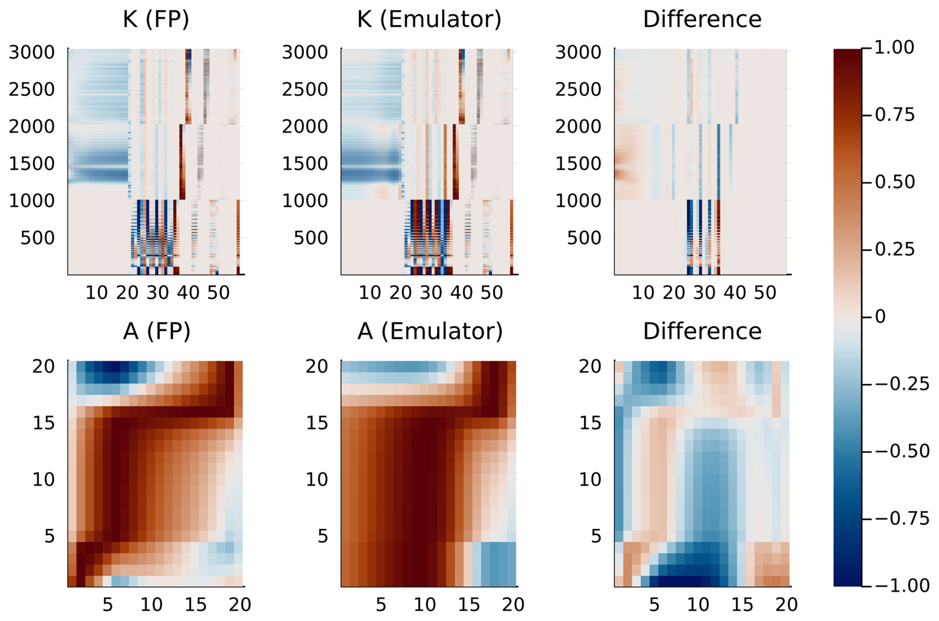
Figure 10 Normalized Jacobians K and profile averaging kernels A from both the FP model and the emulator, together with the corresponding differences.

As noted in previous work by Ma et al. (2019), an emulator provides substantial appeal in terms of computational efficiency. For the current work, the average computational times for model evaluation and Jacobians are summarized in Table 2 on a 2023 MacBook Pro. It is worth mentioning that ReFRACtor computes Jacobians via automatic differentiation, while our emulator does this analytically. Three cases are contrasted: the standard ReFRACtor FP evaluation, the emulator for monochromatic radiances plus ILS, and the emulator alone.

Table 2 Evaluation times of the radiative transfer (RT) model and related Jacobian, comparing the ReFRACtor implementation, monochromatic emulator with instrument line shape (ILS) and other spectral corrections, and monochromatic emulator only.

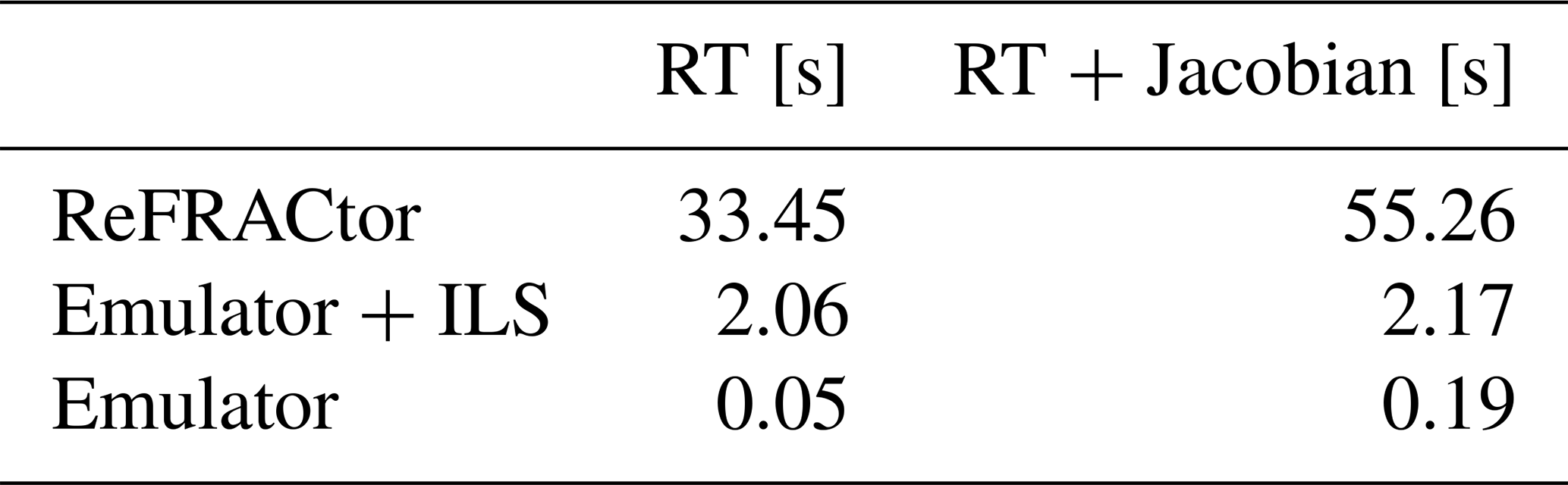
4.4 Faster research version

In recent years, the uncertainty quantification and statistics community has benefited enormously by utilizing the surrogate model by Hobbs et al. (2017) to explore the OCO-2 retrieval in numerous applications (Brynjarsdóttir et al., 2018; Lamminpää et al., 2019; Nguyen and Hobbs, 2020; Hobbs et al., 2021; Patil et al., 2022). We remark that for similar purposes, our emulator can be used as an even faster surrogate. As we see from Table 2, the majority of the computational cost for the emulator comes from the instrument effects, which are part of the ReFRACtor software. If one is not interested in including the effects of dispersion, SIF, and EOFs during the retrieval, we notice from Eq. (10) that instrument corrections to RT amount to multiplication, addition, and convolution, which is associative with respect to multiplication. We can then write the emulator as

$$\begin{array}{}\text{(21)}& g\left(\mathit{x}\right)=\text{ILS}\left(\widehat{\mathbf{P}}\mathit{\eta }\left(\mathit{x}\right)\right)=\text{ILS}\left(\widehat{\mathbf{P}}\right)\mathit{\eta }\left(\mathit{x}\right),\end{array}$$

where g(x) is the overall emulator, ILS() is a function applying the instrument corrections from Eq. (10), $\widehat{\mathbf{P}}$ is a projection matrix consisting of radiance basis functions that correspond to transforming predicted labels z back to radiances y following the last step in Fig. 6, and η(x) is the emulator predicting labels z from inputs x. Done this way, we can evaluate the instrument corrections on the basis vectors once, after which OE or MCMC can proceed an order of magnitude faster (according to Table 2).

5 Retrievals using the emulator

We are now ready to compare the performance of the emulator against the FP model when performing simulated retrievals. After obtaining the minimizer $\widehat{\mathit{x}}$ and a Laplace approximation of posterior covariance, $\widehat{\mathbf{S}}$, the quantity of interest is further given by multiplying the CO₂ profile by the pressure weighting function h that puts an appropriate weight for each pressure level, resulting in

$$\begin{array}{}\text{(22)}& {\text{XCO}}_{\mathrm{2}}={\mathit{h}}^T{\widehat{\mathit{x}}}_{\mathrm{1}:\mathrm{20}}.\end{array}$$

The reported uncertainty coming with the quantity of interest (QoI) is given by

$$\begin{array}{}\text{(23)}& {\text{XCO}}_{{\mathrm{2}}_{\text{uncert}}}=\sqrt{{\mathit{h}}^T{\widehat{\mathbf{S}}}_{\mathrm{1}:\mathrm{20},\mathrm{1}:\mathrm{20}}\mathit{h}}.\end{array}$$

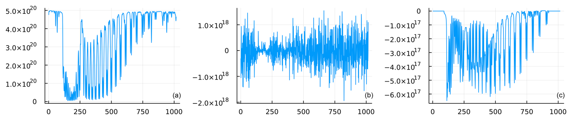
Figure 11 (a) Example O₂ band radiance. (b) Realization from the noise distribution N(0,S_ε). (c) Realization from the model discrepancy distribution N(μ_δ,S_δ). Units for all panels are W m⁻² sr⁻¹ µm⁻¹, the units of radiance for OCO-2.

We present two test cases for assessing retrieval performance of our emulator. First, we create synthetic observations by evaluating the FP model on our test set of states x and by adding a realization from the Gaussian noise distribution:

$$\begin{array}{}\text{(24)}& {\mathit{y}}_{\text{test}}=F(\mathit{x},\mathit{b})+\mathit{\epsilon },\end{array}$$

where $\mathit{\epsilon }\sim N(\mathrm{0},{\mathbf{S}}_{\mathit{\epsilon }})$. Second, we follow the methods outlined in Braverman et al. (2021) to further corrupt the simulated measurement by realistic model discrepancy (MD) adjustment, given by

$$\begin{array}{}\text{(25)}& {\mathit{y}}_{\text{test}}=F(\mathit{x},\mathit{b})+\mathit{\epsilon }+\mathit{\delta },\end{array}$$

where $\mathit{\delta }\sim N({\mathit{\mu }}_{\mathit{\delta }},{\mathbf{S}}_{\mathit{\delta }})$. The shape of this adjustment is illustrated in Fig. 11. As noted by the authors, model discrepancy as presented here is a statistical representation of forward modeling mismatches so that our simulated measurements would better correspond to real data.

We then perform XCO₂ retrievals both using the full-physics model F(x) and the emulator g(x) following the algorithm laid out in Sect. 3. Results for retrieved XCO₂ for both cases with and without MD are illustrated in Fig. 12. The corresponding XCO₂ uncertainty values are compared in Fig. 13. We conclude that using the emulator in place of the FP model in retrieval preserves the accuracy and replicates the same biases as the FP model while having a good correlation with each other. On the other hand, the output uncertainty estimates do not seem to correspond to each other, and further analysis on this output will be required in future research work.

Figure 12 Retrieved XCO₂ over the holdout data set using the FP model and the emulator. Full-physics model (a), the emulator (b), and comparison of the two (c). (d, e, f) Similarly but with added model discrepancy in observed data. RMSE (root mean square error) describes the bias of the retrievals, while the R² value is included to assess the correlation between quantities of interest.

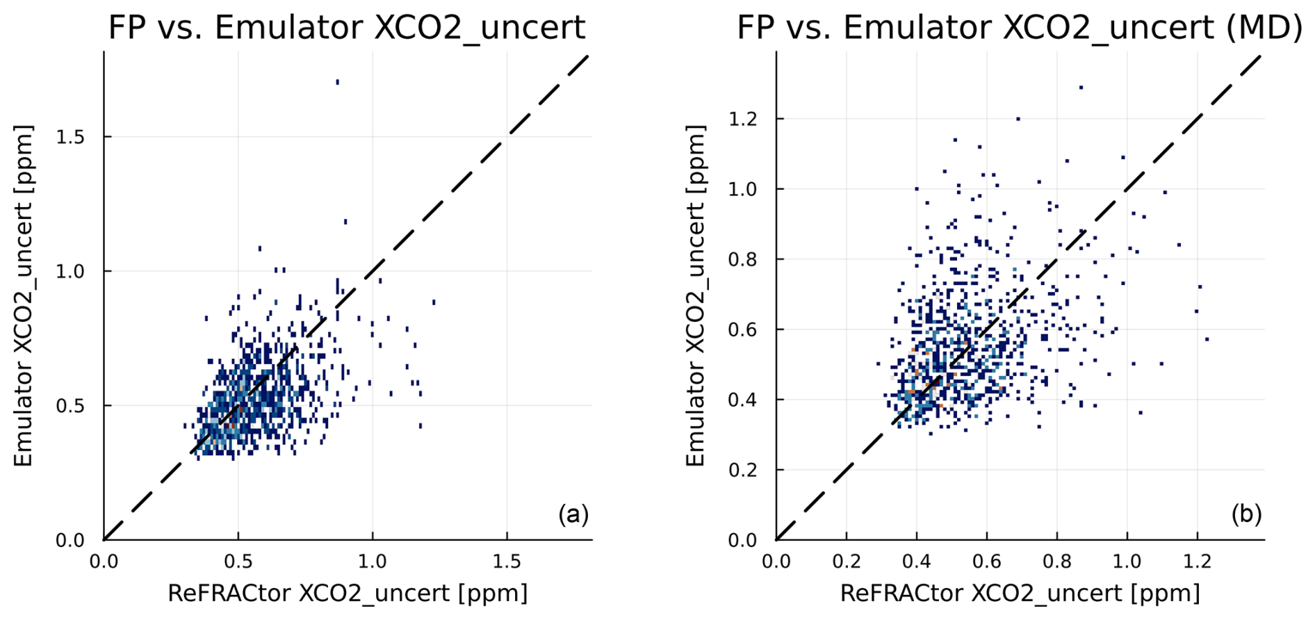
Figure 13 Scatterplots of retrieval XCO₂ uncertainty over the holdout data set using the FP model and the emulator. (a) No MD in observations. (b) MD included in observations.

5.1 Effect of PCA dimensionality

Previously in this work we did not prescribe a certain number of principal components to use in radiance dimension reduction. Figure 14 illustrates the retrieved XCO₂ root mean square error (RMSE) and mean absolute error (MAE) against the true known value, together with Fig. 15, illustrating radiance reconstruction and prediction RMSE and MAE similarly to Figs. 5 and 9, all as a function of the number of PCs used. We can collectively deduce that using more than 25 principal components per band does not yield any additional performance benefits. We remark that compared to the earlier work by Ma et al. (2019), who argued for one to three principal components per band, our results show that many more components are needed for accurate retrievals. This highlights the importance of empirically checking the effect of dimensionality reduction and not relying on rules of thumb such as conserving 95 % of the variability.

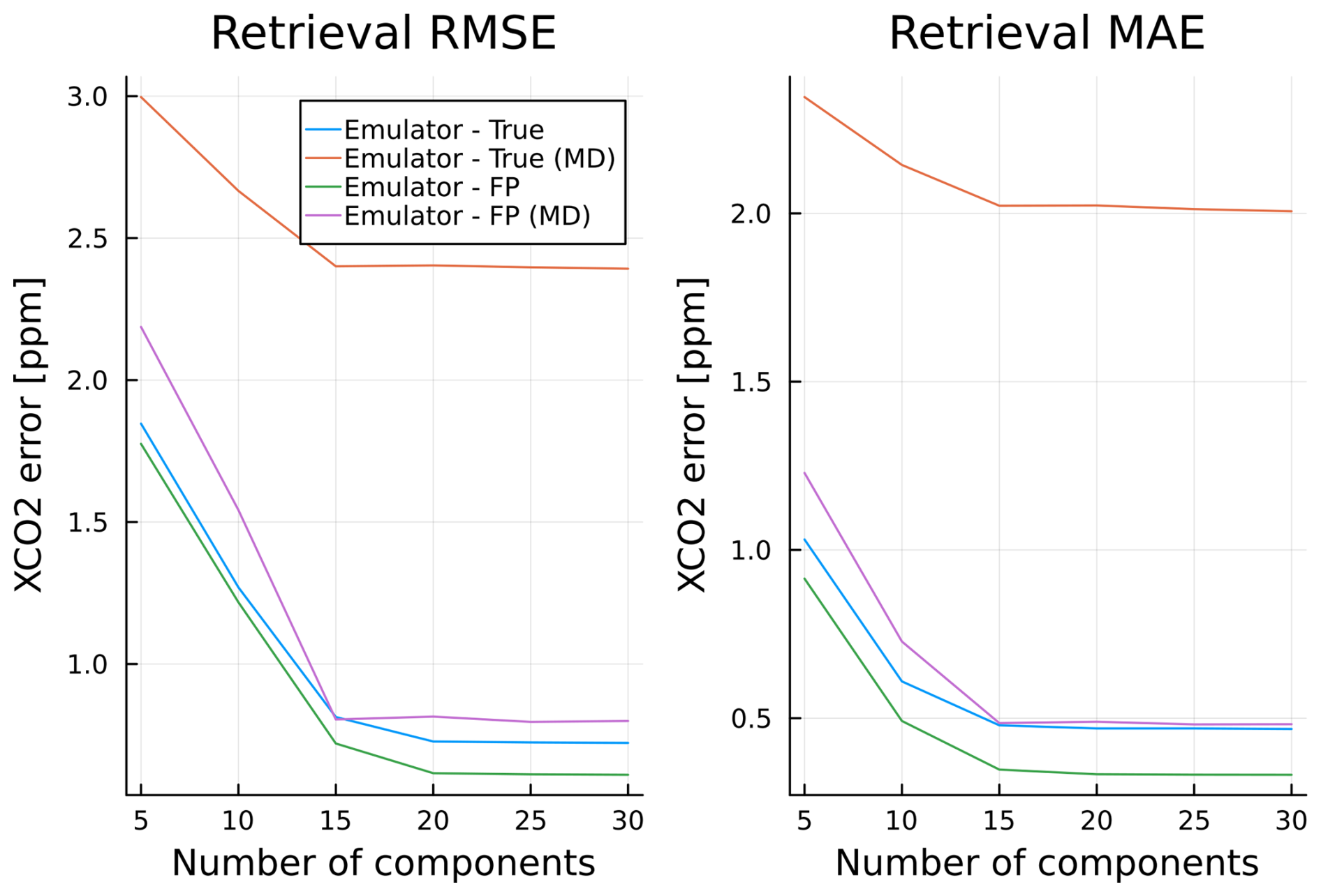
Figure 14 RMSE and MAE as a function of the number of principal components used per band in radiance dimension reduction for XCO₂ retrievals, both with and without MD, over a holdout test data set.

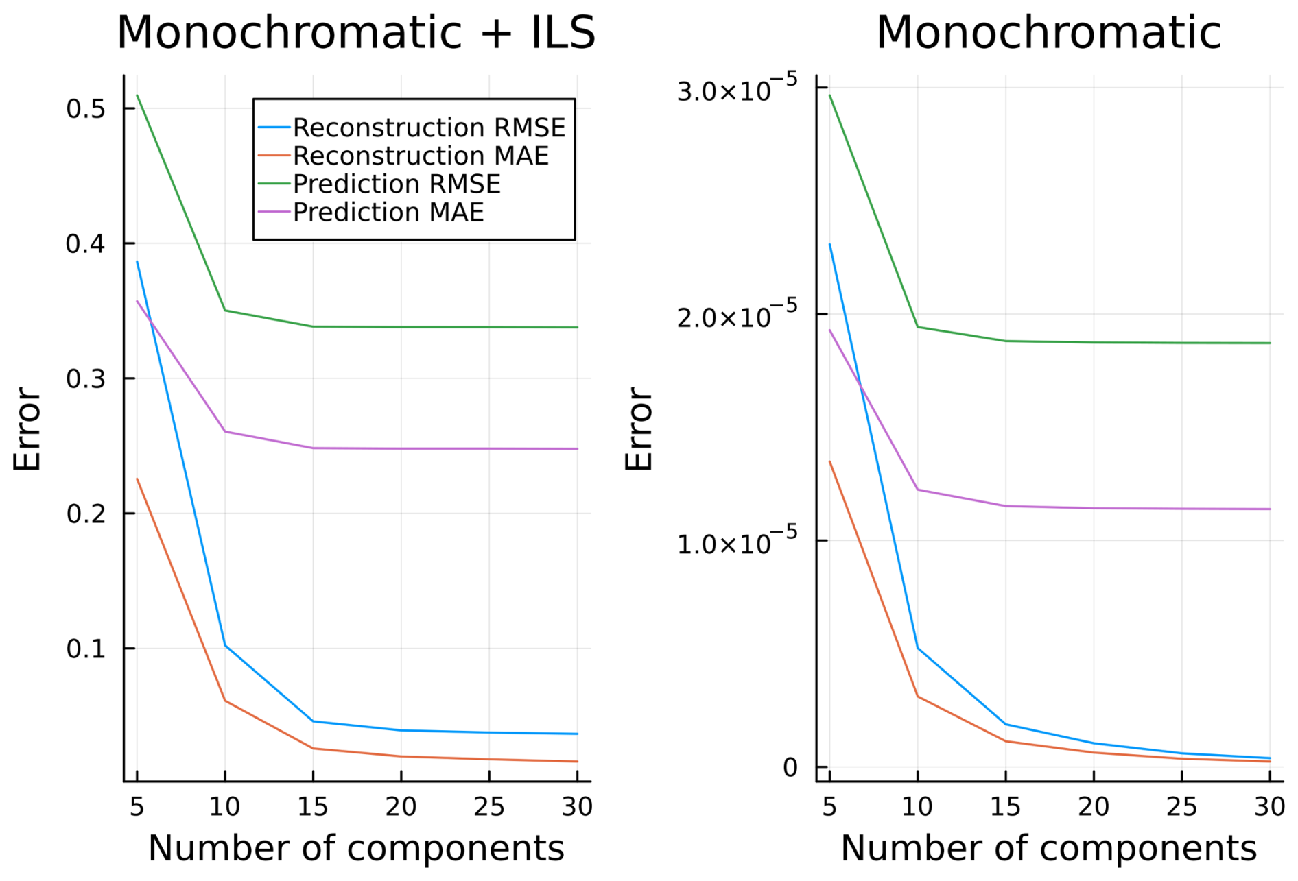
Figure 15 RMSE and MAE as a function of the number of principal components used per band in radiance dimension reduction reconstructions and predictions, all over a holdout test data set.

5.2 Effect of aerosol types

To assess the effect of changing the dominant aerosol types on the performance of the retrievals, we repeat the training and retrieval procedure described in this section with two separate pairs of dominant aerosol types. Firstly, we consider dust (DU) and sea salt (SS) and, secondly, DU and sulfate (SO). These are among the most common aerosol combinations encountered in the OCO-2 operations. We repeat the retrievals for both cases with additional MD adjustment as before. Results of this experiment are summarized in Fig. 16. We conclude that the proposed method is robust in changing physical conditions, which indicates fitness for further operational integration.

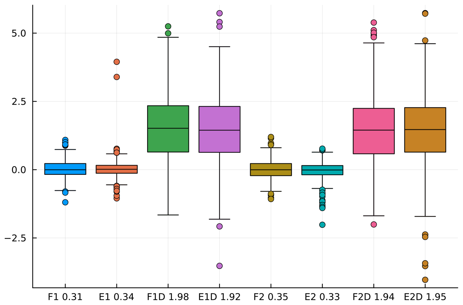
Figure 16 Difference (in ppm) between true and retrieved XCO₂ from simulated measurements with different dominant aerosol species (in ppm). Symbols on the x axis denote the specifics of a given experiment: F – full-physics model, E – emulator, 1 – DU and SS aerosols, and 2 – DU and SO aerosols. D denotes model discrepancy, followed by a number denoting mean error (in ppm).

6 Conclusions

In this work, we have constructed and implemented a fast and accurate forward model emulator for the ReFRACtor implementation of the OCO-2 full-physics forward model. The emulator produces closed-form Jacobians and, as such, provides a convenient way of performing XCO₂ retrievals. We have demonstrated the accuracy of these retrievals and analyzed the effect of PCA dimension, aerosol types, and model discrepancy on the retrieval. All these tests indicate robustness and excellent reliability of our method and offer an encouraging proof of concept for future operational implementation with the latest ACOS algorithm and real-world OCO-2 data.

This work has significantly advanced kernel flow methodology (Owhadi and Yoo, 2019) by including a cross-validation-based training strategy using a RMSE cost function and a new strategy for mini-batching. With this method, we have achieved a relative error of less than 1 %, which on its own is a significant improvement from the point of view of operator learning (e.g., see Batlle et al., 2023, for comparisons of GP and NN methods on various nonlinear problems). Our approach is computationally fast and, when a training data set is properly engineered, performs consistently with the span of training data. Compared with our ability to compute Jacobians in closed form, our approach holds potential to solve current and future data processing issues in atmospheric remote sensing stemming from computationally intensive forward models.

While Gaussian process methods offer an attractive means of including uncertainty propagation in emulation pipeline, our tests have shown that the predicted posterior standard deviation given by GPs was not adequate in providing reliable coverage of true labels after prediction. This is likely due to the kernel flow method's focus on optimizing the posterior mean prediction without assessing the prediction uncertainty. This could easily be remedied by including an uncertainty tuning penalty in the kernel flow loss function. Another disclaimer comes from evaluations of retrieval uncertainty in XCO₂: our method did not agree with operational OE. This does not mean our estimates were better or worse, and further research is needed in calibrating retrieval uncertainties.

A logical next step would be to implement the GP emulator for an operational ACOS forward model instead of ReFRACtor, which requires closer collaboration with the OCO algorithm team. After demonstration on OCO-2, our approach is directly applicable for a myriad of other satellite missions. We note that future work will have to deal with training data design that was simplified in this work. Assessing different temporal and spatial variability in forward model parameters together with feasible distributions of state vectors will be key in this design effort. These efforts might benefit from including a cost–benefit analysis on training a global model usable everywhere versus, for example, retraining the emulator for sufficiently specified spatiotemporal data sets.

Appendix A: Closed-form Jacobians

To obtain a closed-form equation for the Jacobians used in the XCO₂ retrievals, we must explicitly compute the term $\frac{\text{d}}{\text{d}{\mathit{x}}^{*}}\mathbf{\Gamma }({\mathit{x}}^{*},\mathbf{X})$ in Eq. (3). To accomplish this, we compute the partial derivative of the kernel function (Eq. 4) with respect to the first input:

$$\begin{array}{}\text{(A1)}& {\displaystyle }\begin{array}{rl}& {\displaystyle \frac{\partial }{\partial \mathit{x}}}k(\mathit{x},{\mathit{x}}^{\prime })\\ & ={\displaystyle \frac{\partial }{\partial \mathit{x}}}[{\mathit{\alpha }}_{\mathrm{1}}\left(\mathrm{1}+{\displaystyle \frac{\sqrt{\mathrm{3}}}{l}}\Vert (\mathit{x}-{\mathit{x}}^{\prime }){\Vert }_{\mathcal{W}}\right)\exp \left(-{\displaystyle \frac{\sqrt{\mathrm{3}}}{l}}\Vert (\mathit{x}-{\mathit{x}}^{\prime }){\Vert }_{\mathcal{W}}\right)\\ & +{\mathit{\alpha }}_{\mathrm{2}}\left(\mathcal{W}\mathit{x}{)}^T\right(\mathcal{W}{\mathit{x}}^{\prime }\left)\right]\end{array}\text{(A2)}& {\displaystyle }\begin{array}{rl}={\displaystyle \frac{\partial }{\partial \mathit{x}}}& \left[{\mathit{\alpha }}_{\mathrm{1}}\exp \left(-{\displaystyle \frac{\sqrt{\mathrm{3}}}{l}}\Vert (\mathit{x}-{\mathit{x}}^{\prime }){\Vert }_{\mathcal{W}}\right)\right]\\ & +{\displaystyle \frac{\partial }{\partial \mathit{x}}}\left[{\mathit{\alpha }}_{\mathrm{1}}\left({\displaystyle \frac{\sqrt{\mathrm{3}}}{l}}\Vert (\mathit{x}-{\mathit{x}}^{\prime }){\Vert }_{\mathcal{W}}\right)\exp \left(-{\displaystyle \frac{\sqrt{\mathrm{3}}}{l}}\Vert (\mathit{x}-{\mathit{x}}^{\prime }){\Vert }_{\mathcal{W}}\right)\right]\end{array}\text{(A3)}& {\displaystyle }+{\displaystyle \frac{\partial }{\partial \mathit{x}}}\left[{\mathit{\alpha }}_{\mathrm{2}}\left(\mathcal{W}\mathit{x}{)}^T\right(\mathcal{W}{\mathit{x}}^{\prime })\right]\text{(A4)}& {\displaystyle }\begin{array}{rl}={\displaystyle \frac{\partial \mathit{d}}{\partial \mathit{x}}}{\displaystyle \frac{\partial }{\partial \mathit{d}}}& \left[{\mathit{\alpha }}_{\mathrm{1}}\exp \left(-{\displaystyle \frac{\sqrt{\mathrm{3}}}{l}}\mathit{d}\right)\right]+{\displaystyle \frac{\partial \mathit{d}}{\partial \mathit{x}}}{\displaystyle \frac{\partial }{\partial \mathit{d}}}[{\mathit{\alpha }}_{\mathrm{1}}\left({\displaystyle \frac{\sqrt{\mathrm{3}}}{l}}\mathit{d}\right)\\ & \exp \left(-{\displaystyle \frac{\sqrt{\mathrm{3}}}{l}}\mathit{d}\right)]+{\displaystyle \frac{\partial }{\partial \mathit{x}}}\left[{\mathit{\alpha }}_{\mathrm{2}}\left(\mathcal{W}\mathit{x}{)}^T\right(\mathcal{W}{\mathit{x}}^{\prime })\right]\end{array}\text{(A5)}& {\displaystyle }\begin{array}{rl}={\displaystyle \frac{\partial \mathit{d}}{\partial \mathit{x}}}& [-{\mathit{\alpha }}_{\mathrm{1}}\left({\displaystyle \frac{\sqrt{\mathrm{3}}}{l}}\right)\exp \left(-{\displaystyle \frac{\sqrt{\mathrm{3}}}{l}}\mathit{d}\right)]+{\displaystyle \frac{\partial \mathit{d}}{\partial \mathit{x}}}[{\mathit{\alpha }}_{\mathrm{1}}\left({\displaystyle \frac{\sqrt{\mathrm{3}}}{l}}\right)\\ & \exp \left(-{\displaystyle \frac{\sqrt{\mathrm{3}}}{l}}\mathit{d}\right)-{\mathit{\alpha }}_{\mathrm{1}}{\left({\displaystyle \frac{\sqrt{\mathrm{3}}}{l}}\right)}^{\mathrm{2}}\mathit{d}\exp \left(-{\displaystyle \frac{\sqrt{\mathrm{3}}}{l}}\mathit{d}\right)]\end{array}\text{(A6)}& {\displaystyle }+\left[{\mathit{\alpha }}_{\mathrm{2}}\left(\mathcal{W}{)}^T\right(\mathcal{W}{\mathit{x}}^{\prime })\right]\text{(A7)}& {\displaystyle }={\displaystyle \frac{\partial \mathit{d}}{\partial \mathit{x}}}\left[-{\mathit{\alpha }}_{\mathrm{1}}{\left({\displaystyle \frac{\sqrt{\mathrm{3}}}{l}}\right)}^{\mathrm{2}}\mathit{d}\exp \left(-{\displaystyle \frac{\sqrt{\mathrm{3}}}{l}}\mathit{d}\right)\right]+\left[{\mathit{\alpha }}_{\mathrm{2}}\left(\mathcal{W}{)}^T\right(\mathcal{W}{\mathit{x}}^{\prime })\right]\text{(A8)}& {\displaystyle }\begin{array}{rl}={\displaystyle \frac{\mathcal{W}\left(\mathcal{W}\right(\mathit{x}-{\mathit{x}}^{\prime }\left)\right)}{\mathit{d}}}& [-{\mathit{\alpha }}_{\mathrm{1}}{\left({\displaystyle \frac{\sqrt{\mathrm{3}}}{l}}\right)}^{\mathrm{2}}\mathit{d}\exp \left(-{\displaystyle \frac{\sqrt{\mathrm{3}}}{l}}\mathit{d}\right)]\\ & +\left[{\mathit{\alpha }}_{\mathrm{2}}\right(\mathcal{W}{)}^T\left(\mathcal{W}{\mathit{x}}^{\prime }\right)]\end{array}\text{(A9)}& {\displaystyle }={\mathcal{W}}^{\mathrm{2}}\left[-{\mathit{\alpha }}_{\mathrm{1}}{\left({\displaystyle \frac{\sqrt{\mathrm{3}}}{l}}\right)}^{\mathrm{2}}\exp \left(-{\displaystyle \frac{\sqrt{\mathrm{3}}}{l}}\Vert (\mathit{x}-{\mathit{x}}^{\prime }){\Vert }_{\mathcal{W}}\right)(\mathit{x}-{\mathit{x}}^{\prime })+{\mathit{\alpha }}_{\mathrm{2}}{\mathit{x}}^{\prime }\right].\end{array}$$

After computing $\frac{\partial }{\partial \mathit{x}}k(\mathit{x},{\mathit{x}}^{\prime })$, we get $\frac{\text{d}}{\text{d}{\mathit{x}}^{*}}\mathbf{\Gamma }({\mathit{x}}^{*},\mathbf{X})$ element by element, with x being the new input and x^′ a training data point. The final Jacobian is then obtained by computing $\frac{\text{d}}{\text{d}{\mathit{x}}^{*}}{z}^{*}$ via Eq. (3) and reversing transformations in Eqs. (19) and (20).