An algorithm to retrieve peroxyacetyl nitrate from AIRS

Herein, we describe an approach to retrieve free tropospheric columns of peroxyacyl nitrates (PANs) from radiances observed by the Atmospheric Infrared Sounder (AIRS). AIRS has provided daily global coverage since its launch in 2002, making the AIRS data a valuable long term record. Although the instrument is very radiometrically stable, the radiance noise level is large enough to present a challenge when retrieving a weak absorber such as PAN. To address this, spectral windows were selected to minimize interference from other species as much as possible and a set of filters was developed to predict whether a PAN value retrieved from AIRS is within 0.2 ppb or 50 % of what would be retrieved from the Cross-track Infrared Sounder (CrIS) and to remove spurious signals caused by specific surface features or clouds. We show that AIRS is capable of retrieving PAN plumes with very high concentrations of PAN (such as those from significant wildfires) that have similar spatial extent as seen by CrIS and that PAN retrieved from AIRS has good correlation with CrIS given sufficient averaging. We conclude with recommendations for users to help ensure that these data are used appropriately.

1 Introduction

Acyl peroxy nitrates (APNs) are a family of air pollutants formed by the reaction of a peroxy radical with NO₂. Peroxyacetyl nitrate (PAN, CH₃C(O)OONO₂) is the most commonly considered member of this family, resulting from the reaction of a peroxyacetyl radical with NO₂ (Singh and Hanst, 1981). PAN exists in equilibrium with its reactants and is more stable at colder temperatures. Because of this, PAN often acts as a temporary reservoir of nitrogen oxides (NO_x), enhancing long range transport of NO_x to downwind regions (e.g., Singh et al., 1986; Moxim et al., 1996; Hudman et al., 2004). In addition to redistributing NO_x and the associated potential for photochemical production of secondary pollutants, PAN itself is toxic to plants and an eye irritant for humans (Gaffney and Marley, 2021).

PAN is neither a criteria air pollutant nor a designated hazardous air pollutant by the United States Environmental Protection Agency (Suh et al., 2000) or the World Health Organization (World Health Organization, 2021). As a result, routine in situ monitoring of PAN is rare. However, targeted campaigns such as the Arctic Research of the Composition of the Troposphere from Aircraft and Satellites (ARCTAS, Alvarado et al., 2010), Western Wildfire Experiment for Cloud Chemistry, Aerosol Absorption, and Nitrogen (WE-CAN Juncosa Calahorrano et al., 2021a), or Fire Influence on Regional to Global Environments and Air Quality (FIREX-AQ, Warneke et al., 2023) include measurements of PAN to more fully constrain the nitrogen cycle in the outflow of the phenomenon of interest for that campaign. Other campaigns focused on measuring background air, such as HIAPER Pole-to-Pole Observations (HIPPO, Wofsy, 2011) or the Atmospheric Tomography Mission (ATom, Thompson et al., 2022) include PAN measurements to quantify its effect on remote air.

Techniques for remote sensing of PAN have been developed in the last two decades. PAN has very similar absorption features to other members of the APN chemical family (e.g., peroxypropionyl nitrate, peroxy-n-butyryl nitrate, peroxy-n-valeryl nitrate, peroxyacryloyl nitrate, and peroxycrotonyl nitrate, Monedero et al., 2008). Thus, retrievals of “PAN” are in fact retrievals of a mixture of APNs. However, PAN typically comprises the majority (75 % to 90 %) of APNs in both remote areas (Roberts et al., 1998, 2002; Wolfe et al., 2007; Fischer et al., 2014) and urban plumes (LaFranchi et al., 2009). The fraction may be lower in wildfire plumes; Peng et al. (2021) hypothesize that an unknown APN could explain discrepancies in ${\mathrm{NO}}_x/\mathrm{CO}$ ratios between their observations and model. Given the predominance of PAN as the majority APN, the convention is to refer to the satellite products as retrieving “PAN” or “PANs”, and we adopt that convention for this manuscript.

PAN has been retrieved from ground-based instruments as well as limb- and nadir- viewing space-based platforms. Several sites in the Network for Detection of Atmospheric Composition Change (NDACC) perform retrievals of PAN from ground-based spectra (Mahieu et al., 2021). From space, PAN in the upper troposphere/lower stratosphere has been retrieved from limb measurements from CRyogenic Infrared Spectrometers and Telescopes for the Atmosphere (CRISTA, Ungermann et al., 2016) on board two space shuttle flights in the 1990s, the Michelson Interferometer for Passive Atmospheric Sounding (MIPAS, Glatthor et al., 2007; Moore and Remedios, 2010; Wiegele et al., 2012; Fadnavis et al., 2014; Pope et al., 2016), and Atmospheric Chemistry Experiment-Fourier Transform Spectrometer (ACE-FTS, Tereszchuk et al., 2013). Nadir viewing instruments, such as the Tropospheric Emission Spectrometer (TES, Alvarado et al., 2011; Payne et al., 2014), the Infrared Atmospheric Sounding Interferometer (IASI, Coheur et al., 2009; Clarisse et al., 2011; Franco et al., 2018), and the Cross-track Infrared Sounder (CrIS, Payne et al., 2022), provide the ability to retrieve column amounts of PAN sensitive to the mid-troposphere.

Consistent records of atmospheric trace gas concentrations are essential to monitor how air quality is changing over time. A major challenge in this respect is addressing instrument differences among satellites to produce records spanning multiple decades. The Community Long-term Infrared Microwave Combined Atmospheric Product System (CLIMCAPS) product (Smith and Barnet, 2020, 2023) invested significant effort in applying a consistent retrieval to radiances from both the Atmospheric Infrared Sounder (AIRS) and the various CrIS instruments as well as minimizing cross-correlations between retrieved variables (Smith and Barnet, 2019). Smith and Barnet (2025) discuss an information content approach to minimizing differences in CLIMCAPS retrievals. CLIMCAPS produces records spanning the more than two decades since AIRS launched in 2002 that include profiles of atmospheric temperature, H₂O, CO, O₃, CO₂, HNO₃, and CH₄, but does not include PAN.

The TRopospheric Ozone and its Precurors from Earth System Sounding (TROPESS) project also focuses on applying a consistent retrieval algorithm for various trace gases to radiances from a variety of instruments. This includes thermal radiances observed by AIRS and CrIS, as well as radiances in other parts of the electromagnetic spectrum from the Ozone Monitoring Instrument (OMI) and, in the future, the TROPOspheric Monitoring Instrument (TROPOMI). Cady-Pereira et al. (2024) demonstrated the capability with TROPESS to retrieve NH₃ from both AIRS and CrIS. They validated NH₃ from both instruments against aircraft data and found that, although the retrievals from the two instruments are broadly similar, there are differences in the agreement with aircraft profiles. However, after accounting for the smoothing errors, the biases fall below 1 ppb. Pennington et al. (2025) evaluated O₃ trends in three TROPESS products using thermal radiances from AIRS and CrIS and combined thermal and ultraviolet radiances from AIRS and OMI. They compared these products to ozonesonde data, and found that trends in the bias of the retrieved O₃ were significantly less than the reported O₃ trends.

The ability to retrieve tropospheric columns of PAN from space has enabled scientific studies of various sources of air pollution. Several studies made use of the TES PAN retrievals to investigate factors driving PAN over Eurasia (Zhu et al., 2015; Jiang et al., 2016) and the tropics (Payne et al., 2017) as well as the prevalence of PAN in smoke-impacted air masses over North America (Fischer et al., 2018). Other studies (Zhu et al., 2015; Jiang et al., 2016) found that a combination of seasonal temperature, lightning, biomass burning, and microbial emissions influenced the PAN outflow from Eurasia, while Payne et al. (2017) found that the dominant factors in the tropics were biogenic emissions and lightning, with some influence from biomass burning during the study period. Juncosa Calahorrano et al. (2021b) used PAN retrieved from CrIS to quantify the chemical production of PAN in the outflow from the Pole Creek Fire in central Utah, USA. Shogrin et al. (2023) combined PAN values retrieved from TES and CrIS and found that PAN columns over Mexico City had no trend over a time period when NO₂ columns decreased. Shogrin et al. (2024) used PAN columns retrieved from CrIS to study whether there were statistically significant changes in PAN amounts over eight megacities during the COVID pandemic. They found a mix of increases, decreases, and no change in PAN columns among the megacities. More recently, Zhai et al. (2024) used PAN retrieved from IASI to study transport of PANs across the Pacific and concluded that the effect on ozone in the western US was less than 1 ppb. These studies provide examples of how space-based retrievals of PAN, particularly in synergy with other space-based trace gas observations, can provide valuable information about how the meteorological conditions, episodic events, and dominant chemical regime influence air quality in different regions.

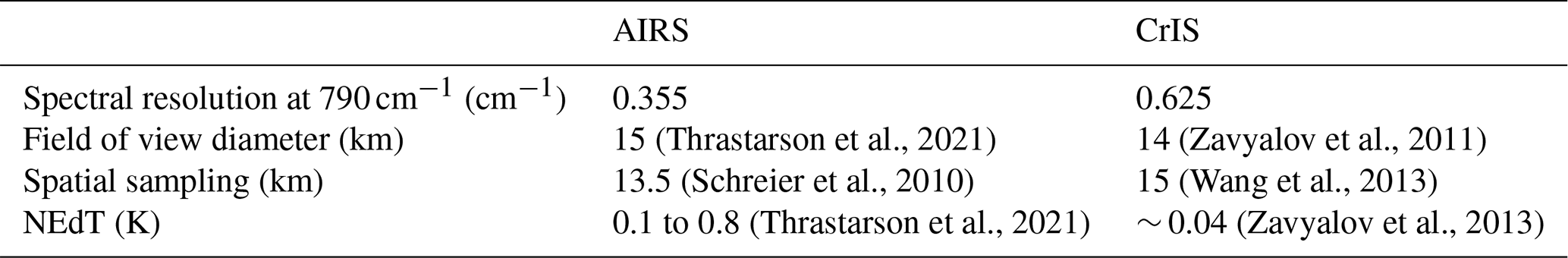
(Thrastarson et al., 2021)(Zavyalov et al., 2011)(Schreier et al., 2010)(Wang et al., 2013)(Thrastarson et al., 2021)(Zavyalov et al., 2013)

Table 1 Comparison of relevant AIRS and CrIS instrument characteristics. Spectral resolution was computed from the L1B files. All other values are from the cited references. NEdT stands for “noise equivalent differential temperature,” and the NEdT value for CrIS was estimated from Fig. 10 of (Zavyalov et al., 2013) for CrIS full resolution spectra.

In this work, we demonstrate the first retrieval of PAN from AIRS. As AIRS was launched in 2002, this has the potential to provide the longest continual record of PAN from a nadir viewing instrument. Our approach is based on that of Payne et al. (2022). We begin with an overview of the AIRS and CrIS instruments, which are both used in this work. Then, we review the MUlti-SpEctra, MUlti-SpEcies, MUlti-Sensors (MUSES) algorithm which provides a retrieval framework for this work. Next, we describe the specific MUSES configuration we use. Fourth, we address several challenges encountered in adapting the approach of Payne et al. (2022) to AIRS spectra. Finally, we close with recommendations to users of the new AIRS PAN product. Due to the computational cost of this retrieval, our analysis focuses on a few days with significant variation in PAN from major fires in the US and Australia. This product will be incorporated in the operational TROPESS data processing in the future (https://disc.gsfc.nasa.gov/information/mission-project?keywords=tropess&title=TROPESS, last access: 11 September 2025), which will enable analysis on a longer timeseries of data.

2 Data sources and algorithm background

2.1 AIRS radiances

The Atmospheric Infrared Sounder (AIRS) instrument is carried on board the Aqua satellite. Aqua was launched in May 2002 and flies in a polar, sun synchronous orbit. For most of its mission, it had a local ascending equator crossing time of ∼ 13:35 LT. Starting in 2022, it began to drift to a later crossing time; as of early 2025, it has an equator crossing time of ∼ 14:30 LT (https://aqua.nasa.gov/, last access: 12 March 2025).

AIRS is a grating spectrometer, covering three spectral bands (approximately 650 to 1140 cm⁻¹, 1220 to 1610 cm⁻¹, and 2170 to 2670 cm⁻¹) with 17 detector arrays and a nominal spectral resolution of $\mathit{\lambda }/\mathrm{\Delta }\mathit{\lambda }$ = 1200 (ranging between 1086 and 1570, Aumann et al., 2003; Thrastarson et al., 2021). The original calibration is described by Pagano et al. (2003) and an update is given in Pagano et al. (2020). AIRS's radiometric calibration has been very stable over its lifetime, with < 2 mK yr⁻¹ drift between 2017 (Aumann et al., 2019) and between −3 and +6 mK since (Aumann et al., 2023). Table 1 compares some of the relevant instrument characteristics of AIRS and CrIS. For a more in-depth description of the differences between the AIRS and CrIS instruments, please see Table S1 of Smith and Barnet (2025) and Table 1 of Smith and Barnet (2019). In this work, we use AIRS level 1B radiances from version 5 of the AIRIBRAD product (AIRS Project, 2020).

2.2 CrIS radiances and the CrIS PANs product

At time of writing, there are three operational Cross-track Infrared Sounder (CrIS) instruments. The first is on board the Suomi-NPP satellite, launched in October 2011, followed by copies on the JPSS-1/NOAA-20 and JPSS-2/NOAA-21 satellites, launched in November 2017 and November 2022, respectively. All three are in sun synchronous orbits with ascending local equator crossing times around 13:30 LT. Unlike AIRS, CrIS is a Fourier transform spectrometer that observes nine fields of view in a 3 × 3 array simultaneously. It performs an across-track scan of 30 view positions. The fields of view are ∼ 15 km in diameter (Zavyalov et al., 2011).

Payne et al. (2022) used radiances from the CrIS instrument on board Suomi-NPP (S-NPP) (specifically the NASA version 2 level 1B radiances, Sounder SIPS and GES DISC, 2017) to retrieve PANs. CrIS measures in three spectral bands: long-wave IR (650 to 1095 cm⁻¹), midwave IR (1210 to 1750 cm⁻¹), and short-wave IR (2155 to 2550 cm⁻¹) (Han et al., 2013). At launch, the CrIS S-NPP instrument was operated in “normal spectral resolution” mode, with the bands measuring at 0.625, 1.25, and 2.5 cm⁻¹, respectively. In December 2014, it was switched to “full spectral resolution” (FSR) mode, with 0.625 cm⁻¹ resolution in all bands (Strow et al., 2021). The NASA FSR level 1B product begins a year later (December 2015) after additional upgrades to CrIS calibration in November 2015. Our work uses the MUSES algorithm (Sect. 2.3), which uses radiances from multiple CrIS bands to retrieve atmospheric trace gases and temperature. Currently, this requires the full spectral resolution product, thus we limit ourselves to CrIS data from December 2015 on.

Payne et al. (2022) validated the CrIS PANs retrievals against PAN measurements taken during the ATom campaign. The measured profiles had GEOS-Chem profiles appended to the top. From the standard deviation of the differences between CrIS and aircraft free tropospheric PAN column averages, Payne et al. (2022) derived a single sounding uncertainty of 0.08 ppb for the CrIS PANs retrieval. This was larger than the uncertainty calculated by the MUSES optimal estimation (OE) algorithm, but Payne et al. (2022) attribute the discrepancy to pseudo-random error contributions from the retrieval of interfering species or the temperature profile. Such interferent-driven error was not included in the uncertainty calculated by the MUSES algorithm, as for PAN retrievals, the algorithm calculates uncertainty from noise only.

Further, the comparison with ATom found a negative bias (CrIS lower than aircraft) that correlated with the total column amount of water vapor. The relationship between water vapor and the CrIS PAN bias was further corroborated by examination of the pre-PAN retrieval spectral residuals, which found a positive residual correlated with water vapor column amounts. From the ATom comparisons, Payne et al. (2022) derived a bias correction for the CrIS PAN product, $c=\mathrm{0.05}+\mathrm{0.035}\times {\mathrm{10}}^{-\mathrm{23}}\times X$, where X is the column density of water vapor in $\mathrm{molec}.{\mathrm{cm}}^{-\mathrm{2}}$ and c is the correction in ppb.

2.3 MUSES Retrieval

The MUSES retrieval (Worden et al., 2007; Luo et al., 2013; Fu et al., 2018; Worden et al., 2019; Malina et al., 2024) is an optimal estimation retrieval with heritage tracing back to the TES retrieval (Bowman et al., 2006). It is instrument-agnostic, able to solve for the optimal state vector given radiances from a variety of instruments (e.g., AIRS, CrIS, the Ozone Monitoring Instrument (OMI), and the TROPOspheric Monitoring Instrument (TROPOMI)), or multiple instruments (e.g., AIRS + OMI, CrIS + TROPOMI).

The MUSES algorithm allows retrievals to be broken down into smaller steps, each of which define the spectral windows for which to minimize the radiance residuals, the atmospheric parameters to solve for, which of those parameters to update for the next step, along with a number of more technical options. The steps are defined in a “strategy table” which can be quickly edited to test different retrieval approaches. This step-wise design provides flexibility to fix some elements of the state vector while updating others in certain steps, which is particularly useful when retrieving state vector elements with large differences in the magnitude of their Jacobian matrices (e.g., atmospheric temperature vs. PAN) or which interfere with each other (e.g., O₃ vs. PAN). These steps are run sequentially; the final state of one step becomes the initial state for the next, save for any state vector elements which the strategy table indicates should not be updated.

Within each step, MUSES uses an iterative solver that applies the trust-region Levenberg–Marquardt scheme (Bowman et al., 2006) to mimimize a cost function

$$\begin{array}{}\text{(1)}& \begin{array}{rl}J\left(\mathit{x}\right)=& [\mathit{y}-\mathit{F}(\mathit{x},\mathit{b}\left){]}^{\mathrm{T}}{\mathbf{S}}_{\mathit{ϵ}}^{-\mathrm{1}}\right[\mathit{y}-\mathit{F}(\mathit{x},\mathit{b})]\\ & +(\mathit{x}-{\mathit{x}}_{\mathrm{a}}{)}^{\mathrm{T}}{\mathbf{S}}_{\mathrm{a}}^{-\mathrm{1}}(\mathit{x}-{\mathit{x}}_{\mathrm{a}})\end{array}\end{array}$$

where

• x is the retrieved state vector,

• x_a is the a priori state vector,

• y is the observation vector (i.e., AIRS or CrIS radiances),

• F is the forward model that simulates radiances given the state vector and fixed parameters (b),

• S_ϵ is the error covariance matrix for the observed radiance, and

• S_a is the prior error covariance matrix.

The Levenberg–Marquardt solver will iteratively update the state vector, x along a direction in state space expected to mimimize Eq. (1). It will continue until the convergence criteria are satisfied or the maximum number of iterations is reached.

An important distinction within MUSES is the difference between the a priori (or constraint) state vector and the initial state vector. The former is x_a in Eq. (1) and is a mathematical constraint on the optimal state vector, the latter is the starting point of x before the first iteration of the Levenberg–Marquardt solver. This distinction is important within MUSES because it is a multi-step retrieval. The strategy table, mentioned above, defines which elements of the state vector will be retrieved in each step and whether or not the retrieved state for step i becomes the initial state for step i+1. For example, the retrieval may begin with an H₂O profile taken from a meteorological reanalysis as both the initial guess and the a priori constraint. An early step in the retrieval can then retrieve a new H₂O profile which is more consistent with the observed radiances. This new H₂O profile can then be used as an initial state for later steps (whether or not those steps retrieve H₂O). This can be important for weak absorbers, such as PAN, which need the profiles of strong thermal IR absorbers to be accurate for the scene in question so that the relatively small absorption feature of the weak absorber can be identified. We note that, for a given step, the initial state and a priori constraint can be the same but do not need to be. For later steps of the retrieval, the initial state may have been set by earlier retrieval steps (as in the example given with H₂O) but the a priori constraint will remain the same for all steps. Or, the a priori constraint may be chosen to be a relatively simple profile to avoid imposing undue assumptions, while the initial state may be chosen to reflect a better estimate of the atmospheric state in that location to attempt to minimize the number of steps needed by the solver.

MUSES can use different radiative transfer models for F in Eq. (1). For this work, we use version 1.2 of the Optimal Spectral Sampling (OSS) model (Moncet et al., 2008, 2015). OSS is designed to use an optimal set of absorption coefficients (per absorbing species and vertical layers) and weights that can be used to compute the radiance for each channel of a spectrometer very efficiently, given the amounts of each absorbing species. These weights are computed by training OSS against a reference line-by-line spectroscopic model. Determining those optimal absorption coefficients and weights requires it to be trained for a given instrument. In version 1.2, the absorption coefficients are calculated from the Line By Line Radiative Transfer Model (LBLRTM) version 12.4 (Clough et al., 2005; Alvarado et al., 2013). This allows OSS to efficiently simulate the radiances a specific instrument would observe by reducing the number of monochromatic wavelengths that must be modeled for a given instrument channel, but means that OSS must be trained for each instrument used in a retrieval separately. For details on the approach, readers are encouraged to review Moncet et al. (2008) and Moncet et al. (2015).

2.4 TROPESS products

The TROPESS project focuses on applying the MUSES algorithm to retrieve a range of atmospheric trace gases from a variety of space-based instruments, including AIRS, OMI, CrIS, and TROPOMI to date. Operational processing for TROPESS is set up to accommodate two distinct goals. The first is to provide a global record of ozone and related trace gases for the first ∼ 20 years of the 21st century. The second is to support rapid iteration on and improvement of the underlying level 2 algorithms while processing more recent data. Due to the computational cost of these retrievals, meeting both goals requires two separate data streams.

The first is a “retrospective” or “reanalysis” stream that retrieves trace gas amounts from ∼ 2002 through ∼ 2021. This stream is processed with a version of the MUSES algorithm frozen at the time the retrospective processing began. The second is a “forward” stream that processes new radiances as they become available with the latest version of the MUSES algorithm, including updates to the algorithm made after the retrospective processing began. The forward stream serves the dual purpose of monitoring significant events affecting air quality and serving as a test bed for improvements to the MUSES algorithm. Due to the difference in the algorithm versions, users must take care not to misinterpret changes in trends between the two streams.

Both streams use a “global survey” sampling approach to process a subset of all available soundings yet provide global coverage, which allows a balance between computational cost and spatial coverage. The default survey strategy processes one sounding in each x° × x° box over land and one out of every four such boxes over ocean. For the current products, x is either 0.7 or 0.8°. In addition, TROPESS produces special collections with full data density for high interest events (e.g., the 2019–2020 Australian Bush Fires and 2020 US West Coast Fires) and a set of megacities around the world.

The CrIS PAN product described in Payne et al. (2022) and Sect. 2.2, with mostly minor updates, is now routinely produced as part of both the reanalysis (Bowman, 2023) and forward (Bowman, 2022) TROPESS streams, as well as special products. The reanalysis and forward streams provide twice daily (day and night) global coverage of PAN, using the global survey strategy described in the previous paragraph. Other species retrieved within the TROPESS project include methane, carbon monoxide, deuterated water (HDO), ammonia, and ozone.

3 AIRS PAN retrieval development

3.1 AIRS PAN retrieval design: microwindows and retrieval order

Retrievals using AIRS radiances have previously been implemented within the TROPESS MUSES algorithm (§ 2.3), thus the AIRS PAN retrieval can use the existing readers and MUSES OE framework. The components that must be added are (1) the desired windows, (2) the strategy table that instructs the MUSES algorithm to retrieve PAN, and (3) details about PAN retrievals copied from the CrIS PAN retrievals, such as the prior vector values.

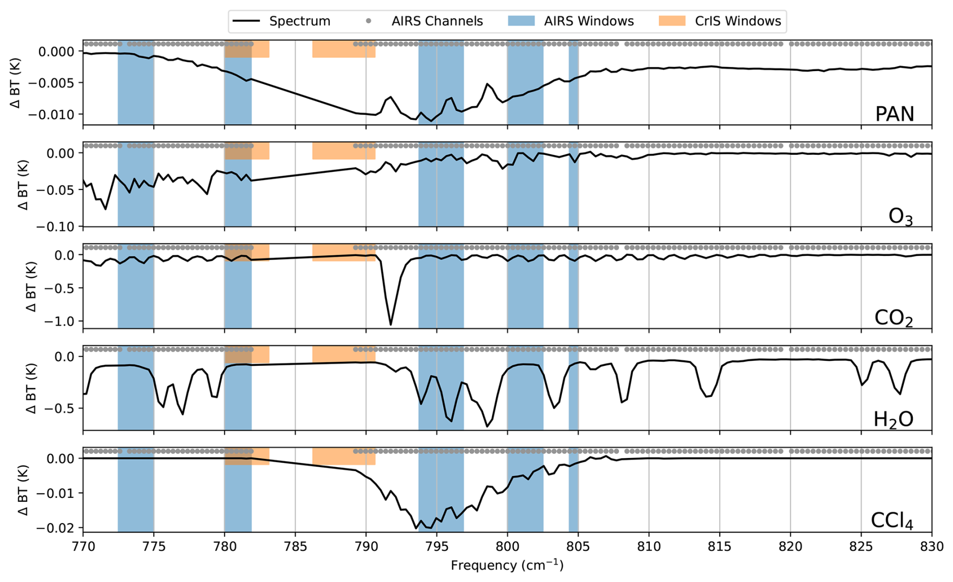
Figure 1 An illustration of the factors driving the selection of windows for the AIRS PAN retrieval. Each panel shows the simulated difference in brightness temperature for a 10 % increase in the mixing ratio of one species at all altitudes as the black line. The AIRS channels are marked at the top of each panel as gray dots. The chosen windows for the AIRS retrieval are the full height blue boxes. For reference, the CrIS windows used by Payne et al. (2022) are the short, orange boxes.

For the existing CrIS PAN retrieval, Payne et al. (2022) chose two windows on the low frequency side of the PAN spectral feature (Fig. 1). However, parts of these windows fall in the AIRS “spectral gap,” where no radiance channels are available. Thus, we had to compromise between windows that will see sufficient signal for PAN absorption and windows that avoid signal from interfering species. Figure 1 shows the selected windows overlaid on simulated absorption features for the relevant species in this spectral range. The two windows on the left of the PAN feature (below 785 cm⁻¹) only see a weak part of the signal from PAN, but are outside of the CCl₄ absorption. The center window at 795 cm⁻¹ is able to capture the core PAN absorption, but has interference from both water and CCl₄. The two rightmost microwindows (above 800 cm⁻¹) are able to avoid interference from water, but have minor to moderate interference from CCl₄. CCl₄ is not retrieved (Table 3) but is simulated in the radiative transfer as an interferent, using climatological profiles scaled by yearly scale factors derived from ground based observations. The base climatological profiles vary with latitude and longitude in 30 and 60° bins, respectively, and were developed from MOZART model output (Brasseur et al., 1998).

Early tests with the three windows above 790 cm⁻¹ showed that omitting the 795 cm⁻¹ window gave erroneously high PAN column average values across much of the western United States during a period when the Pole Creek Fire was emitting PAN (among other species, Juncosa Calahorrano et al., 2021b). Similar tests also showed no benefit to adding additional microwindows above 805 cm⁻¹. The two microwindows below 785 cm⁻¹ were added later to provide the retrieval with some radiance information with PAN but not CCl₄ absorption. The specific frequency ranges for each microwindow are given in Table 2.

Table 2 The microwindows selected for the AIRS PAN retrieval.

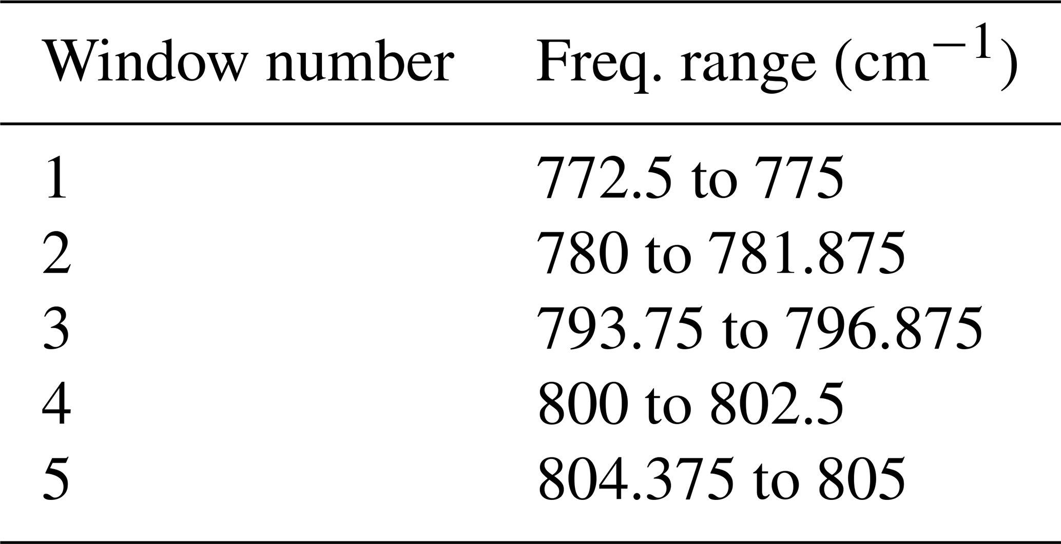
Table 3 The retrieval steps in the strategy table for this AIRS PAN retrieval. Retrieved elements annotated with a ^∗ are only included over land.

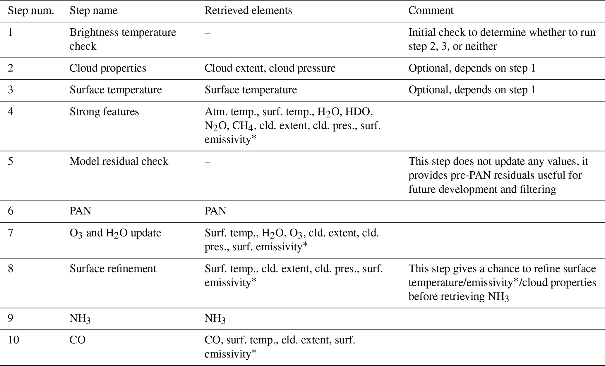
Development of the strategy table was straightforward, requiring only the addition of a PAN retrieval step to the standard AIRS strategy table in use by TROPESS to generate AIRS products. Table 3 enumerates the steps included in this table; the PAN step added is step number 6. The choice to place the PAN retrieval immediately following the “strong features” step (no. 4) follows Payne et al. (2022). Step number 5 was also added to enable saving of spectral residuals in a wider range of frequencies centered on the PAN feature. Such a diagnostic is helpful to understand what factors might be affecting a given retrieval and proved valuable for filtering (Sect. 3.2).

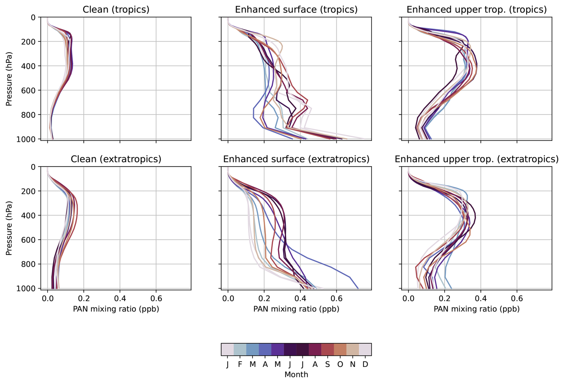
Figure 2 The different sets of PAN mole fraction profiles used as a priori constraints in the MUSES retrieval. Each panel represents a profile type, selected within MUSES based on the sounding location. Within each panel, the variation with month is shown by the differently colored profiles.

The a priori constraints used in the AIRS PANs retrieval are mostly the same as the Payne et al. (2022) CrIS PANs retrieval, with the exception of surface emissivity. As in Payne et al. (2022), the PAN profile used as the a priori constraint for each sounding is selected from a set of 6 climatological profiles for each month (Fig. 2) and the initial PAN profile used as the starting point for the nonlinear optimization is a flat 0.3 ppb in the troposphere. Likewise, the a priori covariance for the PAN VMRs is the same as in Payne et al. (2022). These constraints derive from those used in the retrieval of PAN from the Tropospheric Emissions Spectrometer (Payne et al., 2014). For surface emissivity, we used the Combined ASTER MODIS Emissivity over Land (CAMEL) database (Borbas et al., 2018; Feltz et al., 2018) for our inital and a priori constraint on surface emissivity. Payne et al. (2022) used the University of Wisconsin Cooperative Institute for Meteorological and Satellite Studies High Spectral Resolution database (Borbas et al., 2007). Note that all TROPESS products starting from v1.16 now use the CAMEL database; this included the CrIS PAN retrievals we use for comparison in Sect. 3.3.

3.2 Addressing cloud interference over ocean

During development, we found that low, warm clouds over ocean would be misinterpreted by our AIRS retrieval as PAN. For the cases tested, we were able to filter out such soundings by decomposing the AIRS radiances into empirical orthogonal functions (EOFs) and filtering soundings for which the second principle component (PC) was below a threshold. This section describes that approach.

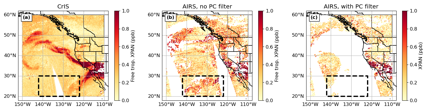
Figure 3 Column average PAN between 825 and 215 hPa as retrieved for 11 September 2020 from both CrIS (on the Suomi-NPP satellite, a) and AIRS (b and c). Compared to (b), (c) uses a PC-based filter instead of the previous retrieval step's water quality check to filter for cloud impacts. The black box in both panels shows the location of the spurious plume in the AIRS retrievals that is the focus of discussion in Sect. 3.2.

This issue of certain clouds appearing as PAN in the retrieval can be seen in Fig. 3, which shows free tropospheric column averages of PAN (which we will refer to as X_PAN) from 11 September 2020. This was a period with major wildfires throughout the west coast of the United States. In Fig. 3a, X_PAN retrieved from CrIS shows a reasonable plume structure, with clear advection of PAN from the fires on the west coast. We also see some of this in the AIRS retrievals – specifically, the enhanced PAN in the southern half of California, most of Arizona, and the northwest corner of Mexico, as well as over the northern Pacific Ocean (Fig. 3b).

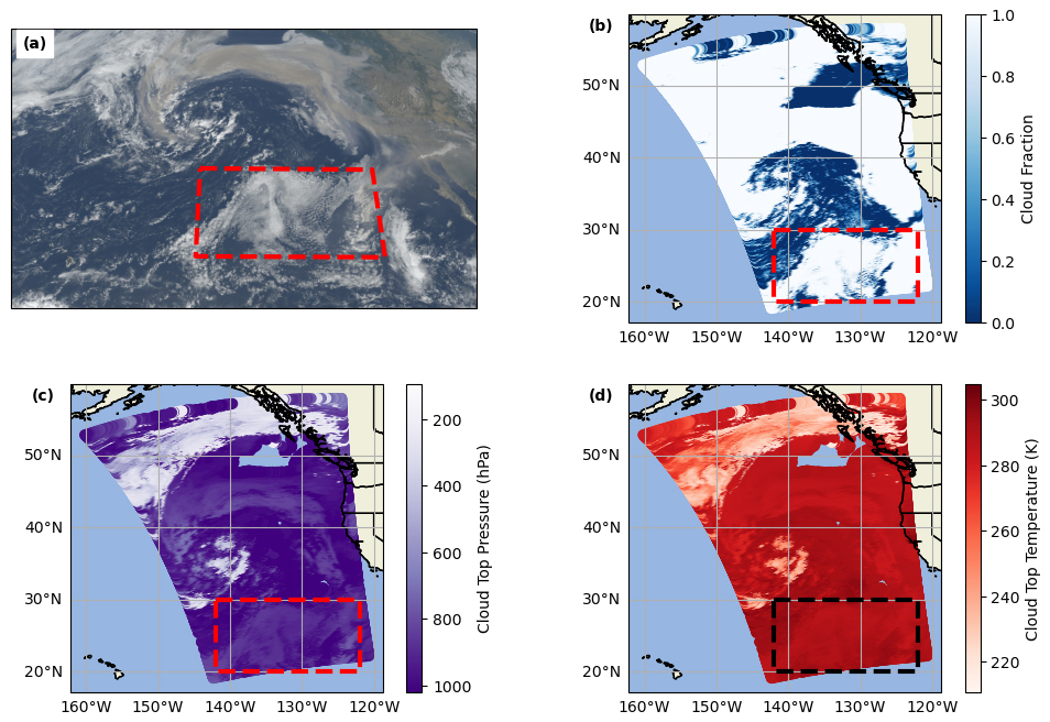
Figure 4 (a) RGB image from the GOES-17 (GOES-West) satellite as captured between 22:11 and 22:13 UTC on 11 September 2020. (b) Cloud fraction, (c) cloud top pressure, and (d) cloud top temperature from the MODIS-Aqua MYD06 product. In all panels, the red or black box encloses the same area as the black boxes in Fig. 3.

However, in the black box (20 to 30° N, 142 to 122° W), CrIS shows mostly background column whereas the AIRS retrievals show an enhancement with an unusual structure (not a shape representative of transport from the fires). When we check RGB imagery from the GOES-West Advanced Baseline Imager (https://noaa-goes17.s3.amazonaws.com/index.html#ABI-L2-MCMIPC/2020/255/22/, last access: 8 December 2022), we clearly see that this “plume” seen by the AIRS PAN retrieval matches the shape of the clouds in that area (Fig. 4a). Further, cloud properties from the MODIS-Aqua MYD06 product (MODIS Atmosphere Science Team, 2017) plotted in Fig. 4b–d show that this is a low, warm cloud. This clear spatial correlation between the cloud extent and the spurious PAN plume leads us to conclude that such low, warm clouds cause difficulties for our retrieval with the chosen spectral windows (Table 2). Similarly, in the plume around 50°N, AIRS sees enhanced X_PAN further west than CrIS (around 150° W) and more to the northwest of the state of Washington (near 50°N, 125°W). From the cloud properties shown in Fig. 4, these are also potential cases of erroneous impact from clouds.

The AIRS data shown in Fig. 3 are those soundings which pass prototype quality flags chosen based on quality flags for other thermal retrievals, including sufficiently small radiance residual, surface temperature > 265 K, cloud top pressure (as retrieved in our algorithm) below the tropopause, and the quality of the H₂O retrieval in step 4 of Table 3. (Note that these quality flags were for prototyping purposes only, and are not those used in the final product.)

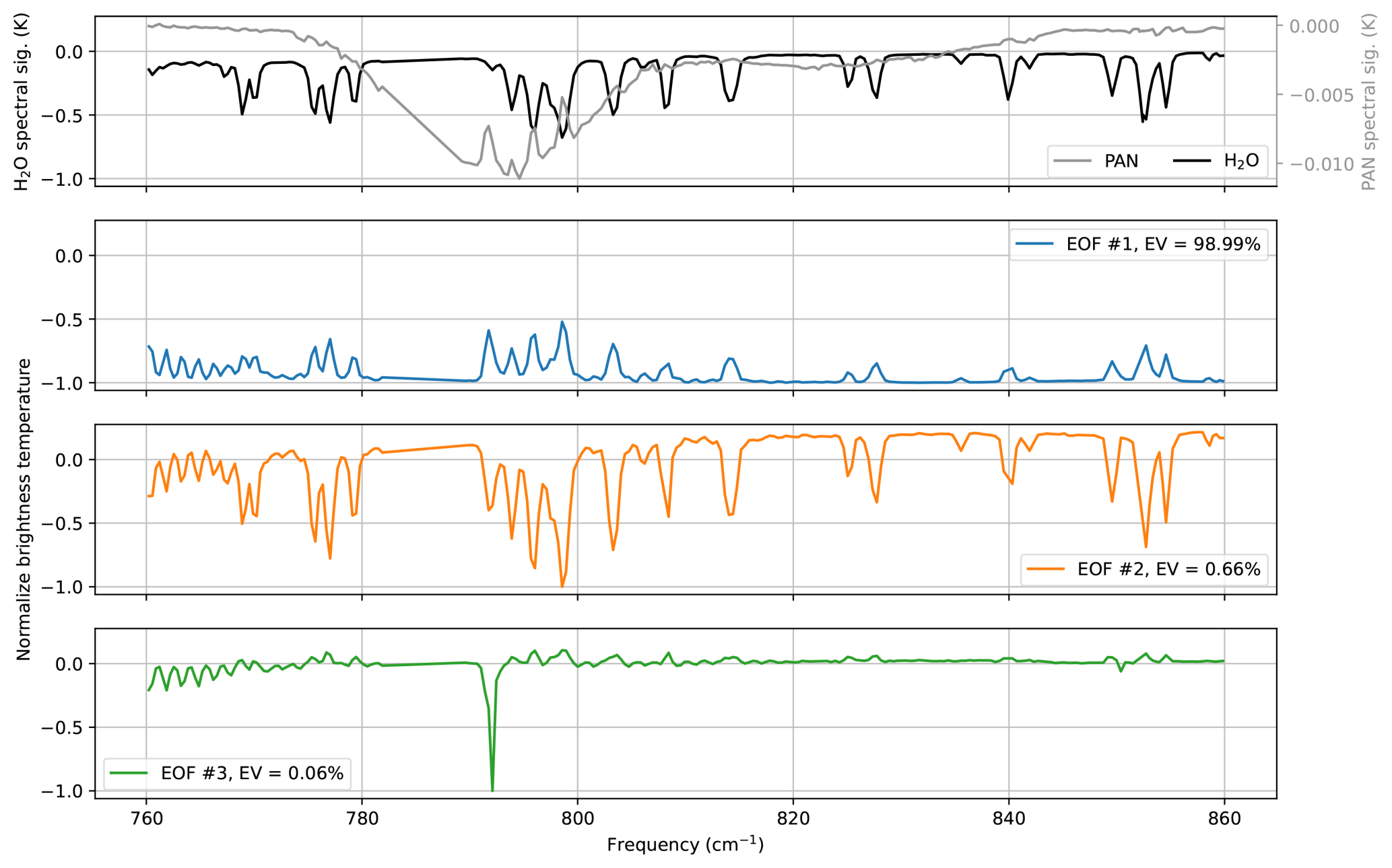
Figure 5 The results of the EOF decomposition on AIRS radiances over a domain covering 20 to 60° N and 150 to 110° W. The top panel shows the spectral signatures of PAN and H₂O from Fig. 1 for references. The remaining three panels show the first, second, and third EOFs, respectively, resulting from the decomposition. The legend in each panel reports the percent of variance explained by that EOF.

Since these criteria were insufficient to remove the spurious plume, we investigated an approach inspired by Huang and Yung (2005). As they used an empirical orthogonal function (EOF) decomposition to study dominant patterns of variability in the AIRS data, we tested whether an EOF decomposition could identify the low, warm clouds causing the spurious PAN signal in our AIRS PAN retrieval. We do note that a cloud-clearing approach, like that used in CLIMCAPS (Smith and Barnet, 2023), could be one approach to address this issue. Such an approach combines radiances from multiple soundings to yield radiances unimpacted by clouds (see Sect. 3 and Fig. 1 of Smith and Barnet, 2025, for a description of this approach) . However, the MUSES algorithm is designed to operate on individual soundings. Therefore, we focused our efforts on the EOF decomposition as a way to screen out these cloud-affected soundings.

Figure 5 shows the first three EOFs resulting from a decomposition of the AIRS observed radiances (as stored by the MUSES algorithm in its output radiance files) within the domain covering 20 to 60° N and 150 to 110° W. Keeping in mind that the sign of an EOF is arbitrary, as it can be flipped by changing the sign of the principal component (PC) by which it is multiplied, the first two EOFs contain many features which match up closely in shape to the H₂O spectral features shown in the top panel. The third EOF appears to relate to CO₂, as the dominant feature appears at approximately the same frequency as the CO₂ feature shown in Fig. 1. These EOFs were computed from the window used in step 5 of the strategy table (Table 3), which spans 760 to 860 cm⁻¹.

Figure 6 The PC values for EOF 1 (left) and 2 (right) for each AIRS sounding in a domain covering 20 to 60° N and 150 to 110° W. The red box in both panels outlines the same area as the black and red boxes in Figs. 3 and 4.

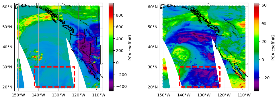
For each AIRS sounding, the observed radiances can be represented as the linear combination of the EOFs with the PCs as the coefficients. Figure 6 shows the values of the PCs for the first two EOFs needed to reconstruct the AIRS radiances for all the soundings in this domain. The second PC (Fig. 6, right panel) has a spatial pattern of negative values strikingly similar to the clouds seen in Fig. 4. In Fig. 3c, we show the AIRS X_PAN with a filter based on the values of PC 2 applied. Filtering out soundings with PC 2 < 0 removes the spurious X_PAN.

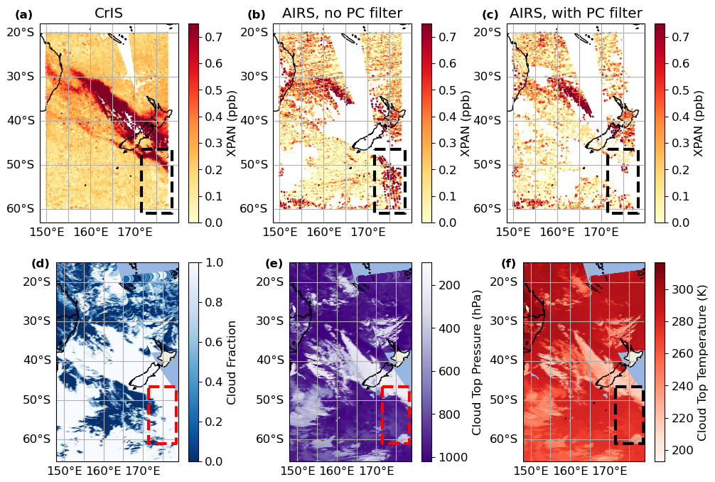
Figure 7 (a) X_PAN retrieved from the CrIS instrument on 1 January 2020 over New Zealand. (b) X_PAN retrieved from AIRS over the same region as (a), with parametric filtering, including a check of the quality of the water retrieval from a previous retrieval step applied. (c) As (b), but with the PC-based filter applied instead of the previous step's water quality check. (d) MODIS-Aqua cloud fraction, (e) cloud top pressure, and (f) cloud top temperature over the same region as (b). In all panels, the black or red box highlights an area with low, warm clouds.

As a next step, we applied this PC-based filtering to different region. We chose a PAN plume from the Australian Bush Fires in late 2019/early 2020. For this Australian fire case, we also see a collection of soundings with large X_PAN values in the AIRS data but not the CrIS data, marked by the black box in Fig. 7a and b. The MODIS cloud properties (Fig. 7d–f) confirm that this is again a low, warm cloud. When we apply the PC-based filter, it correctly marks these soundings as bad quality and removes them (Fig. 7c).

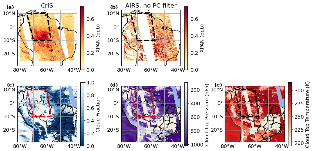
Figure 8 (a) X_PAN retrieved from the CrIS instrument on 11 September 2020 over the Amazon. (b) X_PAN retrieved from AIRS over the same region as (a) without the PC-based filter applied.(c) MODIS-Aqua cloud fraction, (d) cloud top pressure, and (e) cloud top temperature over the same region as (a). In all panels, the black or red box highlights an area where MODIS-Aqua observed mostly low, warm clouds.

Fortunately, it appears that soundings over land are not as susceptible to this issue with low, warm clouds. Figure 8 shows X_PAN retrieved from both CrIS and AIRS again along with MODIS-Aqua cloud properties, this time over the Amazon. While the AIRS X_PAN (Fig. 8b) shows sporadic high values compared to CrIS (Fig. 8a), these erroneous high values appear to be random, rather than systematically located where the low, warm clouds are. In particular, the western swath shows mostly low X_PAN values despite the presence of low, warm clouds. Therefore, we apply the PC-based filter only to ocean soundings.

Our hypothesis is that the reason the AIRS retrieval is affected by the low, warm clouds and CrIS is not is due either the difference in spectral windows used between the retrievals (Fig. 1), the difference in radiance noise between the instruments, or a combination of the two. Further, our hypothesis for why land soundings are much less impacted than ocean soundings is that it is more difficult to distinguish a low, warm cloud from an underlying ocean surface than a land surface.

While the PC-based filter was successful in these cases, we note that it may need additional adjustment in the future. During testing, we found that filtering out soundings with PC 2 < −10 was sufficient for the US West Coast Fires case (Fig. 3), but not the Australian Bush Fires case (Fig. 7), whereas requiring PC 2 < 0 worked for both. Future work will examine whether the criterion of PC 2 < 0 is sufficient globally, or if further refinement is necessary.

We also note that it was necessary to use the 760 to 860 cm⁻¹ window, rather than the narrower windows used in the PAN retrieval step (Table 2). When we tested the latter, this PC-based filter was not effective in the Australian fires case. Therefore, we conclude that information available in the wider window provides the necessary data for the EOFs to correctly fit clouds.

3.3 Filtering and validation through comparison with CrIS

While the PC-based filter addresses the issue of interference from low, warm clouds (Sect. 3.2), it is not sufficient by itself as a quality filter. Ideally, quality filters would be derived by comparing the satellite product to in situ data and checking that the filters ensure good agreement between the satellite and in situ data. To this end, Payne et al. (2022) used aircraft profiles from the ATom campaign to validate the CrIS PAN product. This was ideal for CrIS, as the ATom flights provided profiles of PAN over the majority of the troposphere. However, the majority of the ATom profiles are over ocean (see Fig. 1 of Payne et al., 2022), and this is also true for HIPPO, a similar campaign that occurred before the start of the CrIS FSR product (and so not be used by Payne et al., 2022). As we will lose any profile comparisons that occur over ocean clouds, this would likely limit the number of comparisons we can draw from HIPPO and ATom. To add to the challenge, from Fig. 3, we can see that outside of strong PAN plumes from, e.g., fires, the single sounding retrievals over land from AIRS have significant sounding-to-sounding noise, indicating that bulk statistics will be necessary for a meaningful comparison.

Thus, instead of relying on aircraft data directly, we decided to use the existing CrIS PAN product as a transfer standard by designing a quality filter that predicts whether the AIRS X_PAN value will be within a given threshold of the nearest CrIS X_PAN value. This provides the large number of soundings needed for bulk statistics and implicitly makes the AIRS PAN product consistent with the CrIS PAN product, which can allow users to combine the two.

We chose to implement this quality filter using decision trees, with the Scikit Learn package (Pedregosa et al., 2011). Using simple decision trees allowed us to investigate what variables were used to classify a sounding as good or bad quality during development. Using decision trees rather than hand-tuned quality filter parameters allowed faster iteration and should, in principle, be more reproducible. Because we saw in Sect. 3.2 that ocean soundings required different filtering for clouds than land soundings, we also tested whether using a single decision tree for all soundings or separate decision trees for land and ocean soundings gave better results. We found that separate decision trees for land and ocean soundings retained more soundings with significant X_PAN, and that there was little difference in the correlation between AIRS and CrIS X_PAN using separate land/ocean trees or a single tree. Therefore, we chose to use separate decision trees. Appendix C shows a subset of results using a single decision tree, and describes the trade offs between using a single decision tree and separate decision trees.

Table 4 Regions and dates used for the quality filter decision tree training and testing. A – in the “Training date” column indicates that no data from that region was used in training.

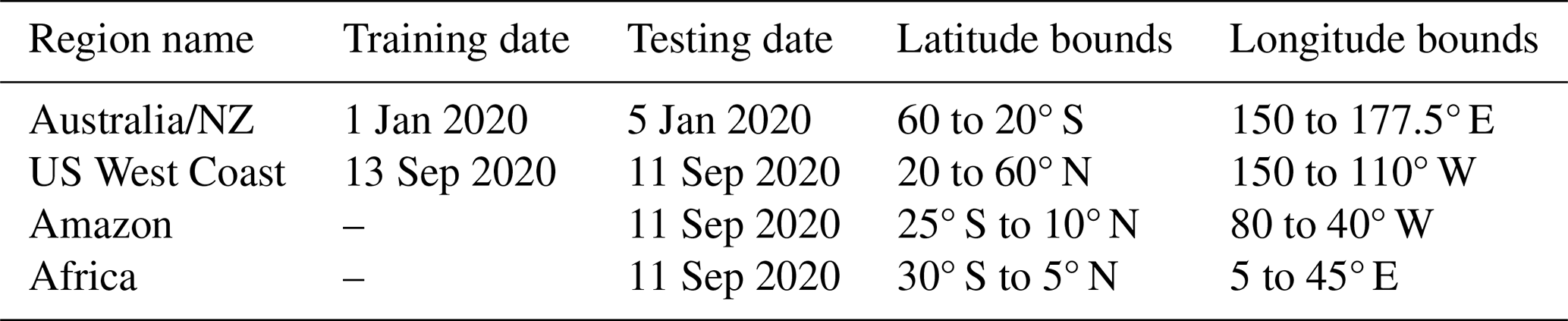
The decision trees were trained on AIRS and CrIS retrievals for one day from each of the 2019/2020 Australian Bush Fires and 2020 US West Coast Fires. Ocean soundings that failed the PC-based filter (Sect. 3.2) were excluded from training. Two different days from these fires, plus retrievals over the Amazon and Africa were used for testing (Table 4). The data was divided into training and testing by days and regions rather than a random $\mathrm{70}/\mathrm{30}$ or similar stochastic split to ensure that the training data included at least some soundings with significant X_PAN. Since plumes with significant X_PAN are outnumbered by background soundings, we were concerned that a fully random split would miss the plume soundings.

Table 5 Input variables for the quality filter decision trees. Note that “O₃ quality” is not useful as O₃ is retrieved after PAN (see Table 3) but is included because it is a standard quality variable in the MUSES algorithm.

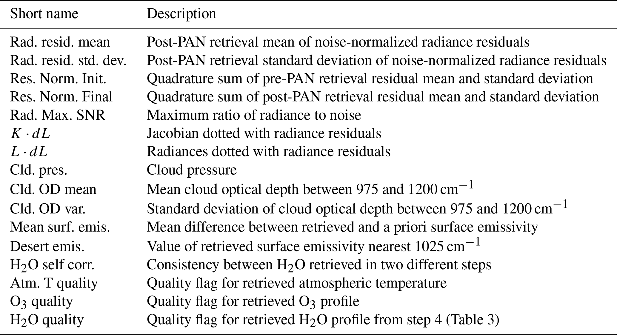
As inputs, the decision trees received 16 values commonly used by existing MUSES retrievals as quality metrics, listed in Table 5. It was trained to predict a binary flag indicating whether the AIRS X_PAN was within 0.2 ppb or 50 % of the CrIS X_PAN from the CrIS sounding closest to it (by great circle distance). The CrIS soundings are restricted to those that pass basic quality flagging for modeled vs. observed radiance and a check for certain surface features that can cause erroneous retrievals. The CrIS X_PAN value compared against includes an averaging kernel adjustment to accommodate different vertical sensitivity between CrIS and AIRS. (see Fig. 15 for a summary of typical CrIS and AIRS X_PAN column averaging kernels.) Specifically, following Eq. (25) of Rodgers and Connor (2003),

$$\begin{array}{}\text{(2)}& {\widehat{c}}_{\text{CrIS},\text{comp}}=c_{\mathrm{a},\text{AIRS}}+{\mathit{a}}^{\mathrm{T}}({\widehat{\mathit{x}}}_{\text{CrIS}}-{\mathit{x}}_{\mathrm{a},\text{AIRS}})\end{array}$$

where

• c_a,AIRS is the a priori X_PAN from AIRS,

• a is the AIRS pressure-weighted column averaging kernel (i.e., one that includes the integration operator),

• ${\widehat{\mathit{x}}}_{\text{CrIS}}$ is the CrIS posterior PAN profile,

• x_a,AIRS is the AIRS prior PAN profile.

Note that the CrIS X_PAN is not an input to the decision trees; it is used only in training. This permits the decision trees to be applied to AIRS soundings without a coincidence CrIS sounding.

Typically, it is important to “prune” decision trees (Esposito et al., 1997) by limiting the number of decision nodes it can include in order to prevent overfitting to the training data. We tested pruning by limiting both the maximum depth (i.e., the number of nodes along any one path) and maximum number of leaf nodes (i.e., the number of end points for the model). However, we found that either method of pruning the decision trees caused the filter to screen out soundings with enhanced X_PAN. Our hypothesis is that, because these soundings are still in the minority of all soundings in the training data, limiting the decision tree's size gave it too little flexibility to account for these somewhat uncommon cases. That is, because soundings with enhanced X_PAN are in the minority, a model limited in size lacked the flexibility to develop useful rules for these soundings, and instead was able to achieve better accuracy by simply classifying all such soundings as bad quality. Therefore, we proceed without limiting the model size.

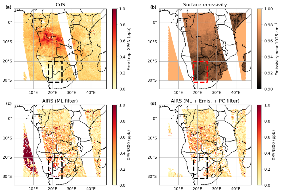
Figure 9 (a) X_PAN retrieved from CrIS on 11 September 2020 over Africa. (b) Surface emissivity at 1025 cm⁻¹. (c) X_PAN retrieved from AIRS with only the decision tree-based filter applied. (d) Like (c), but with the emissivity- and PC- based filters added to the decition tree-based filter. The red or black box in each panel indicates an area with the silicate feature known to bias our PAN retrievals.

Additionally, we include an explicit check that the retrieved surface emissivity at 1025 cm⁻¹ is > 0.94. This filter is similar to one used in Payne et al. (2022) to remove soundings impacted by a silicate feature that produces a surface emissivity with a similar spectral shape to PAN. The same silicate feature also shows up as a low emissivity near 1025 cm⁻¹ (see Appendix B). Although the decision trees are trained on this value as an input, it still retains some soundings clearly affected by the silicate feature. Figure 9 shows CrIS X_PAN in Fig. 9a, AIRS X_PAN in Fig. 9c and d, and the emissivity value in Fig. 9b. The red or black box identifies a region with low 1025 cm⁻¹ emissivity values that has very high X_PAN values in the AIRS retrieval in Fig. 9c. When we add an explicit filter on the 1025 cm⁻¹ emissivity, those few remaining soundings are removed.

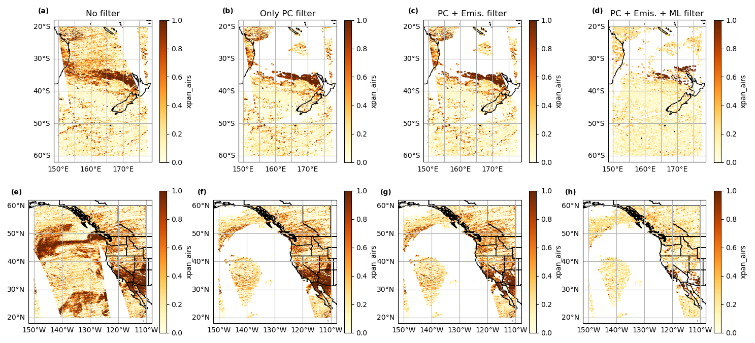
Figure 10 (a) AIRS X_PAN data from the Australian Bush Fires on 5 January 2020 with no filtering applied. (b) As (a), with the PC-based filter applied. (c) As (a), with the PC- and emissivity- based filters applied. (d) As (a), with the PC-based, emissivity-based, and decision tree-based filters applied. (e–h) show the same filtering progression, but for 11 September 2020 over the US West Coast Fires.

The final quality filter will be a combination of the PC-based filter from Sect. 3.2, the emissivity-based filter, and the decision tree-based filter. Figure 10 shows how each of these filters affects the soundings passed as good quality for two days with clear PAN plumes. As discussed in Sect. 3.2, the PC-based filter is applied only to ocean soundings, where clouds cause a high bias in X_PAN. For these two scenes, the emissivity filter has a modest impact, removing some soundings in southern California, northeastern Arizona, and southeastern Utah (Fig. 10g). In both scenes, the decision tree-based filter does remove a number of the soundings with large X_PAN values (Fig. 10d,h). Therefore, in the public files, we will provide the information for users to adjust the quality flagging to suit their application; specifically the PC value used for flagging, the emissivity value used for flagging, and the binary flag produced by the decision trees.

For the rest of this section, we will focus on the performance of the combined filter. Appendix A contains a brief exploration of the relationship between the input variables and predicted quality flag.

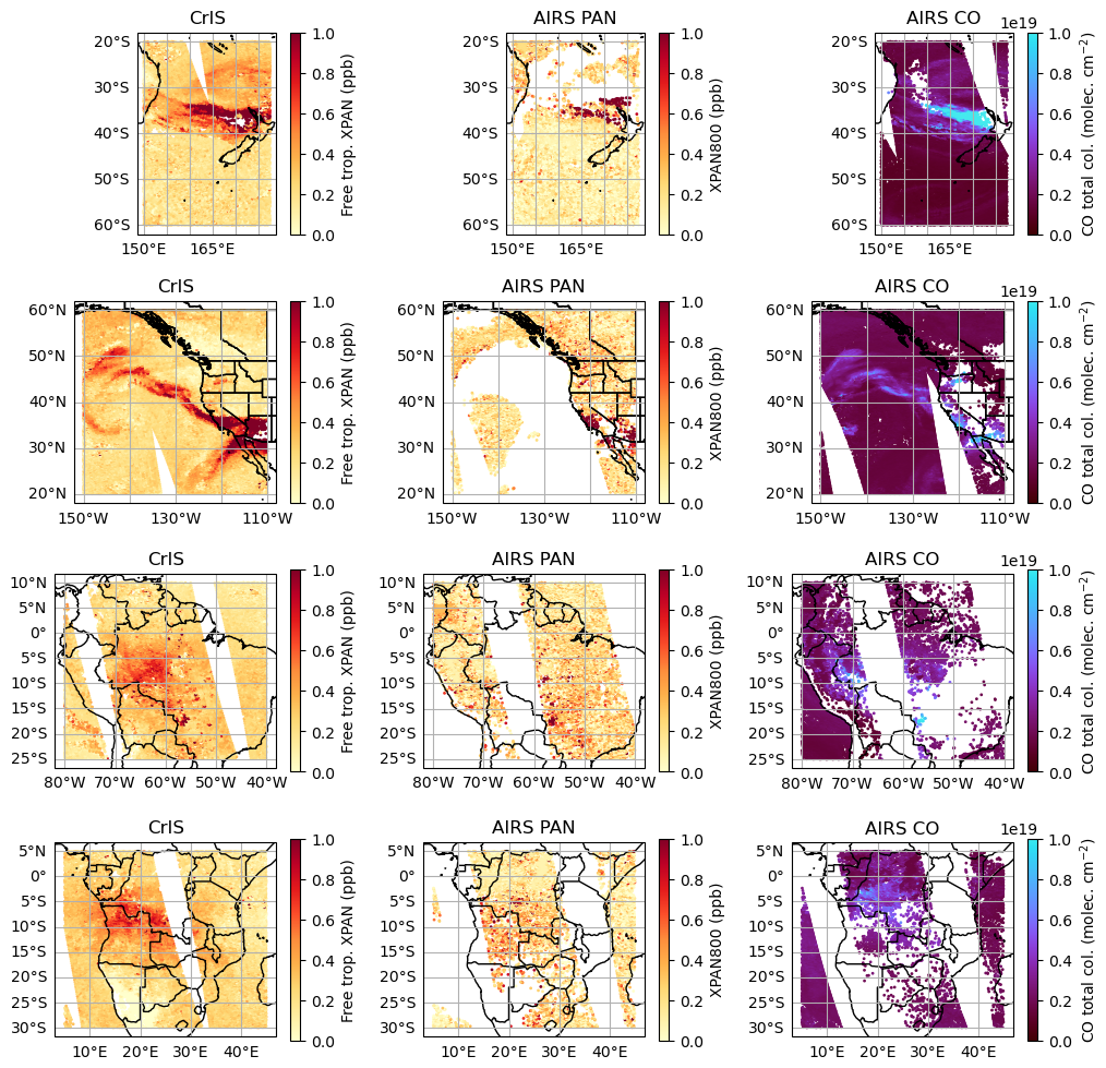
Figure 11 Maps of X_PAN retrieved from CrIS (first column) and AIRS (second column) along with CO total column, also retrieved from AIRS (third column). Each row contains one of the testing region/day pairs from Table 4. The first and third columns are filtered by the standard TROPESS quality flag; the middle column uses the combined decision tree + PC + emissivity filter described in Sect. 3.3.

First, we examine the spatial distribution of PAN plumes in our filtered AIRS product versus CrIS. Figure 11 shows our filtered AIRS PAN data alongside the PAN retrieved from CrIS. The data shown here are from the four testing data region/day pairs in Table 4; thus, these are data that the decision trees were not trained on. The first two rows show the Australian 2019/2020 Bush Fires and the 2020 US West Coast Fires, respectively. In both cases, we can see that the AIRS PAN product matches the location of enhanced PAN plumes seen in the CrIS data very well. In the US West Coast Fires case, the large X_PAN values in Arizona, central/southern California, and northwestern Mexico are all in the same region where CrIS sees high X_PAN values. Likewise, in the Australian fires case, AIRS captures the PAN plume approaching New Zealand's northern island, though compared to CrIS, more of the plume is removed by our filtering criteria.

The last two rows of Fig. 11 show a day over the Amazon and central/southern Africa, respectively. These are regions not included in the training data for the decision trees (Table 4), so these are a good test of whether the filter can generalize to new regions. Neither region has significant PAN plumes in the CrIS data. However, there are small enhancements to ∼ 0.5 ppb in both cases. In the Amazon, there are also a few soundings with ∼ 1 ppb X_PAN near 17.5° S, 55° W. AIRS does see this 1 ppb hotspot, though it also retrieves several soundings with > 1 ppb further north, where CrIS does not. The Amazon hotspot in western Brazil cannot be seen in AIRS due to the swath gap. The PAN hotspot seen by CrIS in the African test over Angola, Zambia, and the Democratic Republic of the Congo is not as apparent in the AIRS PAN; however, AIRS does appear to capture some enhancement in that area, particularly compared to further north, near the equator.

Helpfully, in most of these cases, when there is a strong PAN enhancement in CrIS, AIRS also sees an enhancement in CO. For example, in the Amazon test case, only the soundings with enhanced PAN at 17.5° S, 55° W also have a strong CO enhancement; while the false enhancements further north in the AIRS PAN do not. This implies that users looking for PAN plumes in the AIRS data can check for enhanced CO to distinguish whether a small PAN plume is likely real. This is not a entirely self-sufficient condition, as it is possible to have a PAN plume without enhanced CO, but the presence of enhanced CO can give more confidence in an observed PAN plume. (See Sect. 4 for a summary of recommendations for use.)

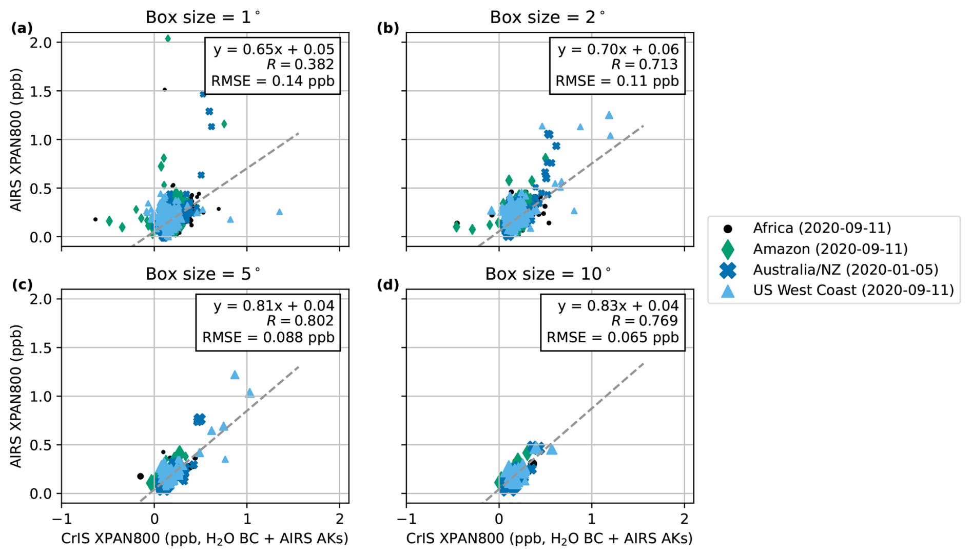
Figure 12 Correlation between AIRS X_PAN and CrIS X_PAN where the latter includes both the AIRS averaging kernel correction from Eq. (2) and the H₂O bias correction from Payne et al. (2022). The different test date/region pairs from Table 4 are represented by the different color series. Each marker represents the daily average of the AIRS and matched CrIS soundings in a box with the size of the marker increasing with the number of soundings in that box. Each box must have a minimum of 10 soundings to be included. The box size is the only difference between panels: (a) 1° × 1°, (b) 2° × 2°, (c) 5° × 5°, and (d) 10° × 10°

We also tested the correlation between AIRS and CrIS X_PAN with different amounts of spatial averaging. Figure 12 shows the results for four different spatial averaging box sizes. While the data from our test cases does have some fire-influenced observations, many of the observations vary primarily from large-scale seasonal or latitudinal variations. At 1° × 1°, the correlation is somewhat weak. The correlation is more significant at 2° × 2°, 5° × 5°, and 10° × 10°. However, averaging to 5° × 5° or 10° × 10° is needed for the root mean squared error (RMSE) between AIRS and CrIS X_PAN values to drop below 0.1 ppb and for the visual correlation (especially for high values) to be apparent. This is a fair amount of averaging, but is not surprising, given the sounding-to-sounding variation seen in Fig. 11. Given the amount of observations, this will still provide useful PAN coverage. We discuss recommendations for use based on this result in Sect. 4.

In Fig. 12d, we see that the AIRS X_PAN value is biased low compared to CrIS X_PAN. It is not clear if this bias in the AIRS data is best parameterized as a function of H₂O, as was the case for CrIS, or if another parameter is a better predictor. Payne et al. (2022) were able to derive the CrIS bias correction through comparison between CrIS and in situ background X_PAN values. In this work, the need to average a significant number of AIRS soundings to reduce the random sounding-to-sounding noise makes it difficult to identify any relationship between AIRS X_PAN values and H₂O column amounts.

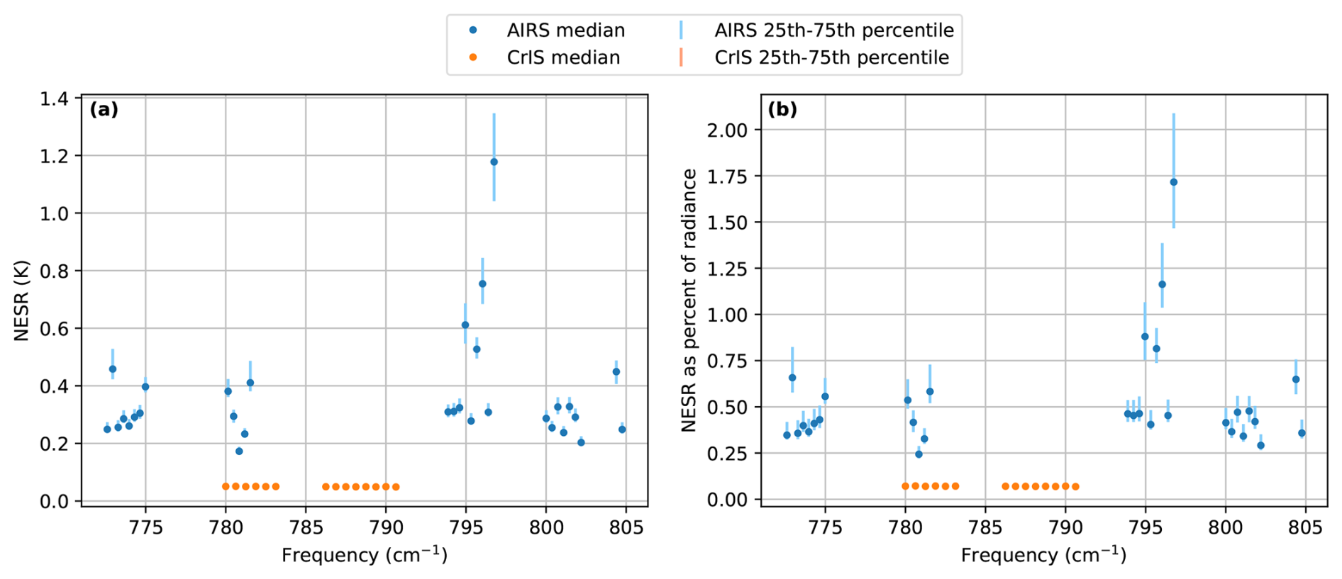
Figure 13 (a) Noise equivalent spectral radiance (NESR) from the channels in the spectral windows used in the CrIS and AIRS PAN retrievals. The circles give the median NESR value per channel and the error bars show the 25th to 75th percentile range. The medians and percentiles are computed over all soundings from the training and test data listed in Table 4. (b) As (a), but with the NESR values given as a percentage of the corresponding observed radiance.

3.4 Uncertainty estimates and vertical sensitivity

The CrIS radiance noise is lower than the AIRS radiance noise, which is a significant advantage when retrieving species, such as PANs, with only weak absorption features. Figure 13 shows per-channel median and 25th to 75th percentile noise equivalent spectral radiance (NESR) values. Although we use different frequencies in the AIRS and CrIS retrievals, the AIRS NESR values are systematically greater than the CrIS values. Taking all of our test cases for comparing AIRS and CrIS (Table 4), we find that the median ratio of AIRS to CrIS NESR across all channels is ∼ 5.9. Assuming that single sounding uncertainty scales linearly with radiance noise, that suggests that the AIRS single sounding uncertainty in X_PAN should be approximately 0.5 ppb, that is, approximately six times the 0.08 ppb value Payne et al. (2022) calculated for CrIS. This aligns with the correlation between AIRS and CrIS X_PAN shown in Fig. 12, which shows that AIRS values below 0.5 ppb are dominated by random uncertainty without significant averaging. We also checked the correlation between individual AIRS and CrIS X_PAN values in Fig. 14, and similarly see that the values have a spread of ∼ 0.5 ppb. While we expect the error of individual soundings to vary depending on the specific atmospheric and surface conditions for each sounding, we believe 0.5 ppb to be a reasonable estimate of the typical uncertainty in the AIRS X_PAN data.

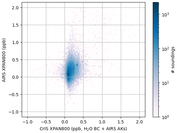
Figure 14 A heatmap showing the distribution of AIRS X_PAN compared to the corresponding CrIS X_PAN with averaging kernel adjustment and H₂O bias correction. Unlike Fig. 12, there is no averaging, this is a comparison of individual soundings.

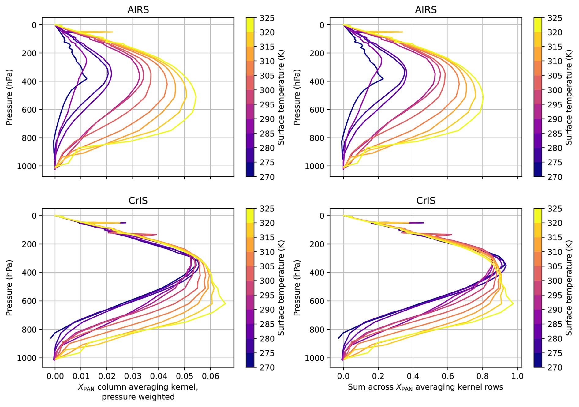
Figure 15 The left two panels (a, c) show column averaging kernels for the free tropospheric column average quantities from AIRS (top) and CrIS (bottom). The values are the dot product of the free tropospheric pressure weighting function with the averaging kernel matrix; thus, the averaging kernels shown are weighted by each level's contribution to the column average. The right panel shows the sum across rows of the averaging kernel (Cady-Pereira et al., 2024). This quantity estimates the sensitivity of the column to a given level, without the pressure weighting function. The kernels shown in all panels are the medians in 5 K surface temperature bins from the good-quality soundings of the US West Coast Fires domain on 11 September 2020. For CrIS, good quality is defined using the standard MUSES quality flag. For AIRS, it uses the PC-based, emissivity, and decision-tree based filters as described at the end of Sect. 3.3.

Figure 15 compares the pressure-weighted column averaging kernels and the sum across the rows of the averaging kernel (Cady-Pereira et al., 2024) for AIRS and CrIS for good quality land soundings within the US West Coast Fires domain on 11 September 2020. The averaging kernels shown are the medians of averaging kernels for soundings binned by surface temperature. For both instruments, maximum sensitivity shifts to lower pressure with decreasing surface temperature. However, compared to CrIS, AIRS maximum sensitivity decreases more quickly as surface temperature decreases. We suspect this is due to the greater noise present in the AIRS radiances, with AIRS sensitivity decreasing more with reduced thermal contrast due to the greater noise. However, we have not confirmed this hypothesis. Note that, for both instruments, the averaging kernels shown in the left panels incorporate the pressure weighting function, which is why the values are well below 1.

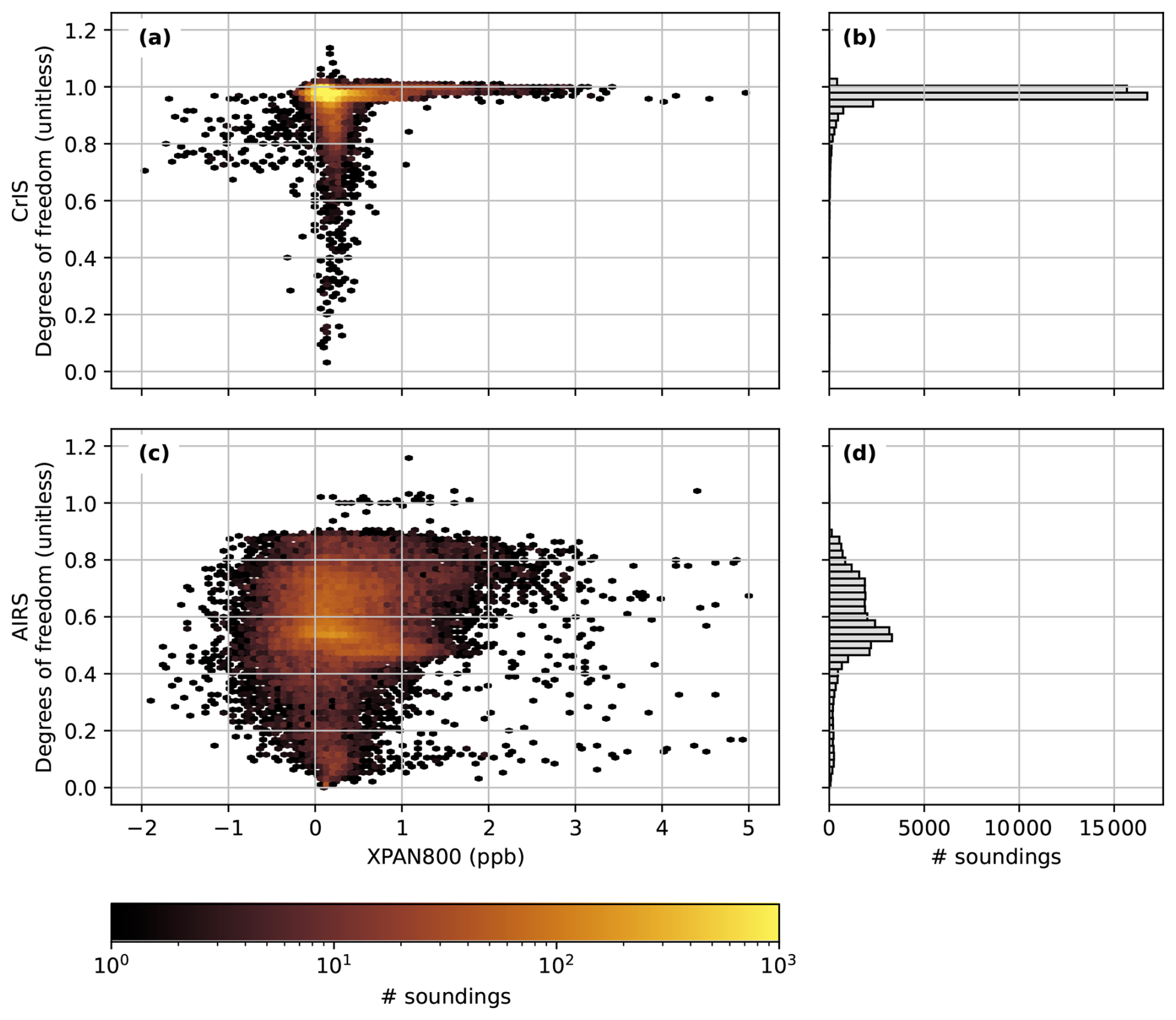
Figure 16 (a) A 2D histogram of degrees of freedom of signal vs. retrieved X_PAN from CrIS. (b) A histogram of the CrIS degrees of freedom. (c) As (a), but for AIRS. (d) as (b), but for AIRS. All panels are from the 11 September 2020 scene over the US West Coast Fires shown in Fig. 3. No soundings were removed by filtering.

Figure 16 shows the overall degrees of freedom (DOF) of signal for both the AIRS and CrIS products in the 11 September 2020 US West Coast Fire scene. From Fig. 16a and b, we can see that the DOFs for the CrIS PAN product are grouped around 1, indicating that there is essentially always enough information to retrieval a single piece of vertical information in the form of a column average. In contrast, Fig. 16c and d show that the AIRS DOFs are lower (centered around ∼ 0.5) with a wider distribution. Greater AIRS X_PAN values do tend to be associated with greater DOFs. This implies that the AIRS product will retain influence from the prior, particularly in background conditions, but can detect sufficiently large PAN enhancements.

4 Recommendations for use

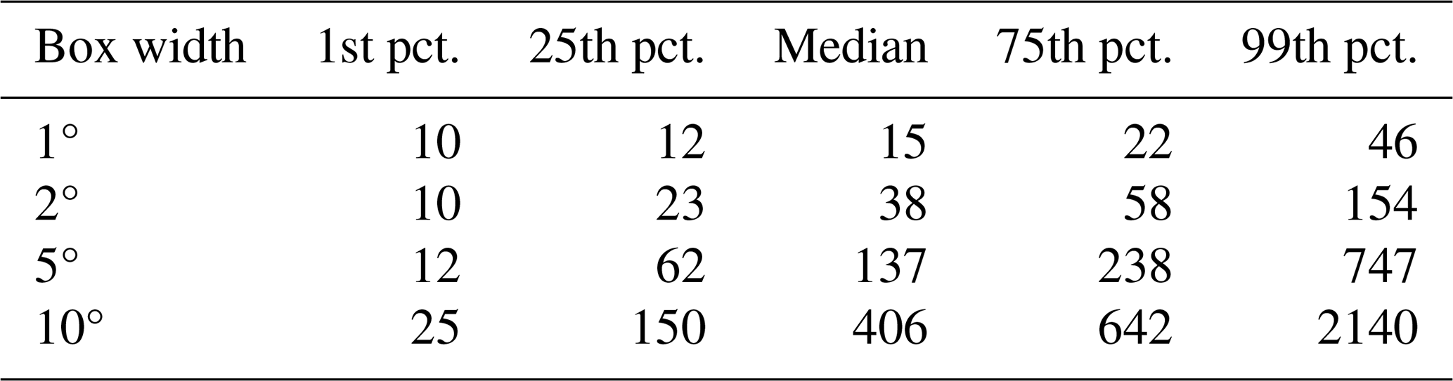
The primary benefit to a retrieval of PAN from AIRS is the longer record available from AIRS compared to CrIS. We envision two primary use cases for this product. The first use case is tracking long term changes in background PAN levels. Given the sounding-to-sounding variation in the AIRS X_PAN values, this will require significant averaging to discern trends in X_PAN from AIRS. However, Fig. 12 does show that the root mean squared error between AIRS and CrIS is < 0.1 ppb when averaged to a 5° × 5° or 10° × 10° box, which is comparable to the CrIS PAN errors. This does not imply that the overall error is < 0.1 ppb (as the AIRS and CrIS retrievals could have similar systematic errors), only that the AIRS and CrIS records will be consistent to within 0.1 ppb with similar averaging. Table 6 gives ranges of the number of points in each box size from Fig. 12. Based on this information, our first recommendation is that users interested in trends in background PAN from the AIRS product choose a spatiotemporal averaging window that has a median of at least 140 soundings passing our quality screening per window which will result in a typical difference versus CrIS of about 0.1 ppb. This is chosen as the median number of points (to two significant figures) in a 5° × 5° box (Table 6), as Fig. 12 shows this box size is sufficient to reduce the RMSE between AIRS and CrIS to < 0.1 ppb. In principle, it should not matter whether the 140 soundings are accumulated by averaging in time or space, as we assume the AIRS-CrIS X_PAN differences are similarly uncorrelated in time as in space. We expect this assumption to hold true as long as episodic events that significantly perturb PAN concentrations (such as wildfires) are not included in the time period averaged. We will test this assumption in the future as more data becomes available.

Table 6 Distribution of the number of points in the different sized boxes used for the AIRS-CrIS comparisons.

The second use case is investigating PAN from extreme events, such as wildfires, before the start of the CrIS PAN product. We showed in Fig. 11 that the AIRS PAN product does reliably see significant X_PAN values of 0.5 to 1 ppb. However, users should be aware that there are many cases where a high AIRS X_PAN value within a small spatial area is false. Figure 14 shows that there is a large fraction of AIRS soundings with X_PAN > 0.5 ppb that match with CrIS soundings with X_PAN < 0.5 ppb. Therefore, users looking for PAN caused by extreme events should

1. ensure that high X_PAN values are spatially connected (as a contiguous plume is more likely to be a real signal than a spurious single-sounding error), and

2. check for other species expected to be generated by the event of interest, such as CO for wildfires.

These two criteria should help users filter out false positive high X_PAN values. When using other species of interest, users need not restrict themselves to TROPESS products – any good-quality dataset will be useful in this regard. Users interested in extreme events with large X_PAN values should note that the decision tree-based filter can remove soundings with clear PAN enhancements. Custom filtering using only the PC- and emissivity- based filters can be used in such cases to recover the soundings with enhanced PAN; however, users must be aware that the difference with respect to CrIS will likely be larger in such a case. Further, while we believe that the PC-based filter is able to remove most cloud-affected soundings, there may be cases where it is not fully effective. Thus, we encourage users to engage with the algorithm team if there is concern about whether a signal of interest in the AIRS PAN is correct. As stated in Sect. 3.4, users should use a 0.5 ppb uncertainty per sounding when using individual soundings in their analysis.

5 Conclusions

We have demonstrated the ability to retrieve free tropospheric column amounts of PAN from AIRS spectra. This is more challenging than the existing CrIS retrieval due to the higher radiance noise in AIRS than CrIS and the presence of a gap in the AIRS spectra on the low-frequency side of the PAN spectral feature. The AIRS PAN retrieval is also sensitive to low, warm clouds over oceans, which cause spurious PAN signals in the AIRS PAN retrieval. These spurious signals have been successfully removed with a PC-based filter in testing, but further adjustment may be needed to make this filter fully effective at removing these signals.

The AIRS product does have larger errors than the CrIS product and requires care in its application. This is mitigated by the use of a decision tree-based quality filter trained to identify AIRS soundings with X_PAN values significantly different than the nearest CrIS sounding and by averaging sufficient numbers of AIRS soundings. For studies of background PAN concentrations, we recommend averaging at least 140 AIRS soundings which will result in a ∼ 0.1 ppb error relative to the existing CrIS PAN product. This product opens up the potential for a global record of free tropospheric PAN amounts from 2002 to the present, potentially allowing the evaluation of trends in background PAN for over two decades.

This product is planned for inclusion in the TROPESS forward stream, provided AIRS continues to operate. This would allow us to evaluate its performance over a larger range of times than was possible during development. Future work could take advantage of that data set to further test the effectiveness of the PC-based filter on the effects of clouds over ocean. This can also enable us to explore alternative methods of retrieving PAN from AIRS taking advantage of, e.g., more advanced machine learning methods trained to directly retrieve X_PAN, that may reduce the sounding-to-sounding noise. An interesting experiment would be to test whether a well-designed machine learning approach could be trained to directly predict the X_PAN value CrIS would retrieve given only the AIRS radiances.

Appendix A: Decision tree explainability

We use SHapeley Addition exPlanations (Lundberg and Lee, 2017) to investigate what values most contributed to the decision trees' prediction of AIRS quality in Sect. 3.3. The results are shown in Fig. A1. Since these are classification decision trees, the SHAP value represents an increase or decrease in the probability of the sounding being classified as “good,” with positive SHAP values indicating a high “good” probability.

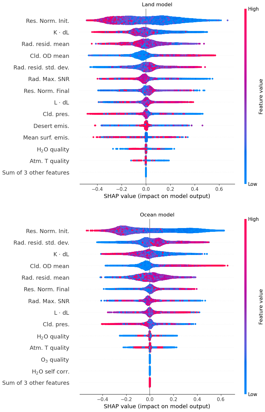
Figure A1 Beeswarm plot showing the Shapley values for the 13 input variables to the quality filtering decision trees that have non-zero contributions to the output flag. The meaning of each input variable's short name is given in Table 5.

Some of the relationships shown in Fig. A1 make physical sense:

• Res. Norm. Init., the pre-PAN residual, follows the expected pattern where smaller residuals are more likely to yield a good sounding. Since this is the pre-PAN retrieval residual, this suggests that a successful retrieval is highly dependent on the previous steps minimizing the observation/model mismatch from other atmospheric parameters. This is a reasonable relationship, as PAN is a weaker absorber than the trace gases optimized in a previous step (Table 3).

• K⋅dL, which represents maximum of the absolute value of the dot product of the residuals with the Jacobian, is essentially a summary of the residual weighted towards frequencies with strong absorbance. Therefore, it is likewise sensible that decreasing values of this quantity increase the chance of a sounding being classified as “good.”

• Rad. resid. mean, the mean of the post-PAN residual, should indicate how well the posterior solution matches the observed radiances. This is also a sensible metric, as it indicates how well the optimization algorithm minimized the cost function, so lower values should correlate with a higher probability of the sounding being marked as good quality, which is what we see in the land model.

Several of the other relationships from Fig. A1 are less clear. For example, mean cloud optical depth and the maximum signal-to-noise (SNR) ratio seem backwards: higher cloud optical depth and lower SNR seem unlikely to correlate with good soundings, as generally more optically thick clouds should obfuscate the radiances of interest and lower SNR spectra should be more difficult to extract a signal from. However, we must remember that these decision trees are trained to predict if AIRS returned X_PAN similar to CrIS. Thus, we interpret this behavior to mean that these are cases where AIRS and CrIS return similar X_PAN values due to these factors. Optically thick clouds likely mean that both instruments are not able to obtain much information about the trace gas columns, and therefore return similar values. Likewise, low SNR spectra will have a low information content, thus both retrievals are more likely to return the prior. Since we use a consistent prior in both retrievals, this would result in similar X_PAN.

Rad. resid. std. dev. shows another unexpected relationship. This is the standard deviation of the post-PAN radiance residuals. Larger values generally indicate that there is a lot of variation in how well the posterior state matched the observed radiances. This can occur if, e.g., narrow features in the radiances were not fit well by the posterior state causing specific frequencies to have large residuals. Interestingly, both models associate greater values with improved likelihood of a sounding being good quality. This may indicate that there are narrower absorption features than PAN which the optimization can try to fit incorrectly with PAN, and thus the decision tree is identifying that soundings were these non-PAN absorption features are not erroneously fit are more likely to be good quality. However, this is speculative. Alternatively, it may be similar to mean cloud optical depth and SNR, where this is simply identifying cases where the posterior is similar to the prior. Since the AIRS and CrIS retrievals use the same prior, this would result in consistent values for the same reasons as mentioned for cloud optical depth and SNR.

For the remaining features, we mostly see them centered on zero impact, with the long tails to either end having a mix of high and low input values. This indicates that there is not a clear correlation between these input values and the predicted quality.

Appendix B: Physical interpretation of emissivity interference

Figure 9 showed that, in the region with low emissivity near 1025 cm⁻¹, very high AIRS X_PAN was retrieved, but CrIS retrievals returned very low X_PAN. These opposed effects of the silicate feature discussed in relation to Fig. 9 arises from the relative shapes of the emissivity and PAN spectral features and the position of the AIRS and CrIS microwindows.

Figure B1a shows the surface emissivity near 1025 cm⁻¹ again, and Fig. B1b shows the spectral shape of the emissivity feature in two boxes marked in Fig. B1a. From this, it is clear how the low emissivity near 1025 cm⁻¹ used in our quality filtering corresponds to a dip in the emissivity in the frequency range of the PAN feature (the gray shading in Fig. B1b). Figure B1c expands the PAN frequency range and shows the emissivity features along with the PAN feature and AIRS and CrIS windows. Due to steps prior to the PAN step, the emissivity versus frequency is set to a straight line between 780 and 810 cm⁻¹ with no fitting inside the 780–810 cm⁻¹ window. We can see that the AIRS windows fall primarily on frequencies where the slopes of the PAN and southern box's emissivity features versus frequency have the same sign. Thus, in AIRS, the silicate emissivity feature present in the southern box is fit by the retrieval as additional PAN, as increasing the absorbance due to PAN will generally reduce the residuals. However, the second CrIS window covers frequencies where the PAN and emissivity features have opposite slopes versus frequency. For CrIS therefore, the retrieval may attempt to invert the PAN feature to produce the concave down shape seen in the emissivity, resulting in negative X_PAN values over regions with this feature.

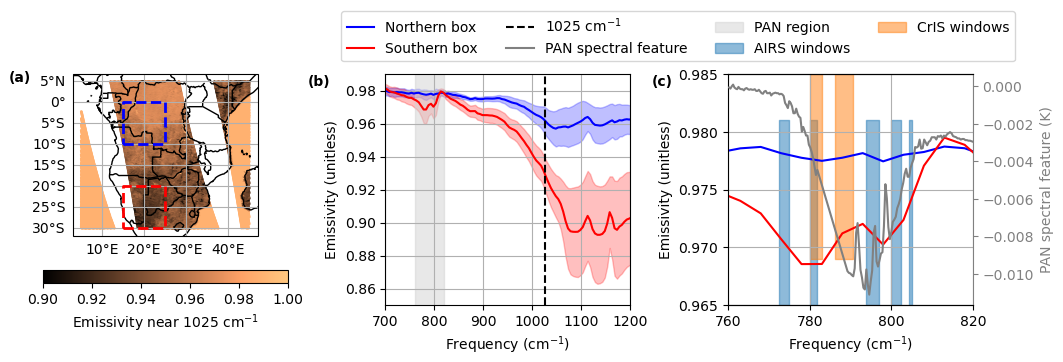
Figure B1 (a) A map of surface emissivity at 1025 cm⁻¹, as in Fig. 9, but with two boxes indicating areas with different emissivity values. (b) Spectral shape of the emissivity values in the two boxes marked on panel (a). The lines indicate the mean emissivity and the shaded areas ± 1 standard deviation within each box. The grey area marks the frequency range plotted in panel (c). (c) The mean emissivity from the same boxes as (b), with the PAN spectral feature and microwindows from Fig. 1 overplotted. The AIRS and CrIS microwindows are offset vertically solely to make them distinguishable where they overlap.

Appendix C: Using a single decision tree for quality filtering

For the decision tree-based filter described in Sect. 3.3, we tested using a single decision tree for both land and ocean soundings instead of separate trees for those two categories of soundings. In principle, a single decision tree would be preferable, as it would both simplify implementation and eliminate concerns that mixed land/ocean soundings or soundings near a coast could be filtered using the less applicable decision tree. This section shows why we elected to use separate decision trees instead.

Figure C1 shows the correlation between AIRS and CrIS X_PAN with different levels of averaging when using the single decision tree in the filter, instead of separate decision trees for land and ocean soundings. Comparison to Fig. 12 shows that, on the gross scale represented by the averaging boxes used here, neither option is clearly better than the other. Using a single decision tree instead of separate trees yields similar R and RMSE values, with the single decision tree performing better at some levels of averaging and the separate trees performing better for others.

However, when we compare Fig. C2 to Fig. 10, we can see in panels d and h that the single decision tree (Fig. C2) removes more of the PAN plumes compared to the separate trees (Fig. 10). This was the main reason we chose to use separate decision trees to filter land and ocean soundings, as the ability to examine plumes from extreme events is one of our primary use cases.

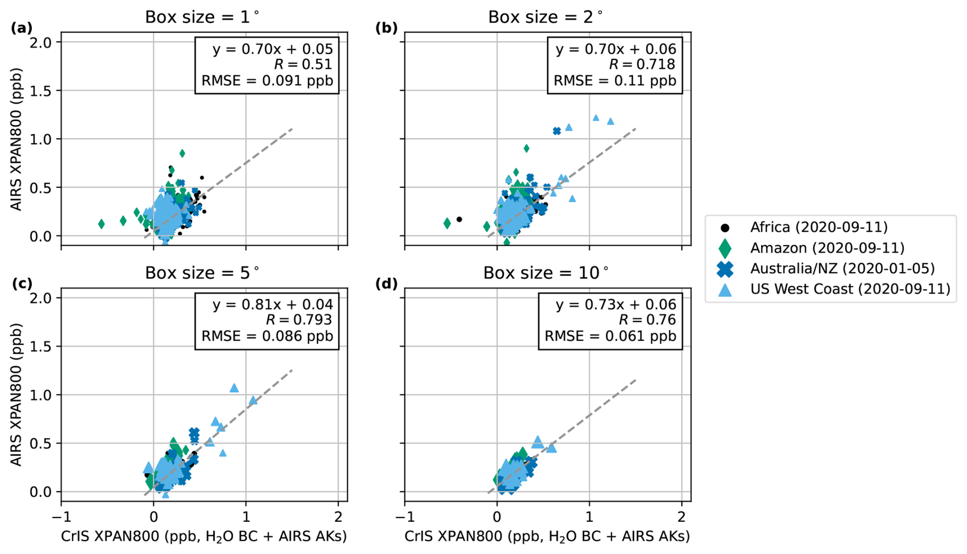
Figure C1 This figure is the same as Fig. 12, except the filtering uses a single decision tree trained on and applied to both land and ocean soundings, rather than separate land and ocean trees.

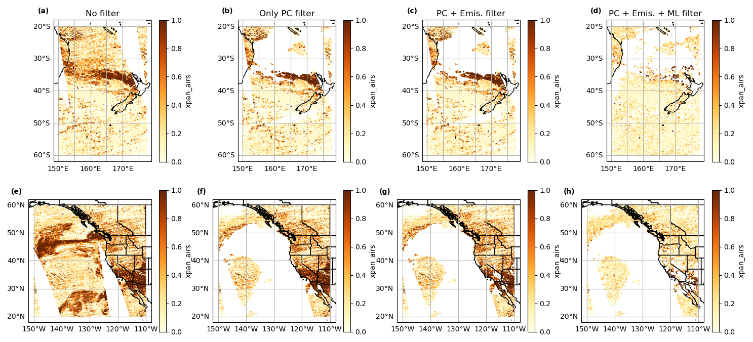
Figure C2 This figure is the same as Fig. 10, except the filtering uses a single decision tree trained on and applied to both land and ocean soundings, rather than separate land and ocean trees.