Uncertainty estimation of aerosol properties from a Vaisala CT25k ceilometer based on in situ aerosol measurements

In recent years, the use of automatic lidars and ceilometers (ALC) for atmospheric research has increased. Originally, these instruments were developed to measure cloud base height automatically, utilising the LIDAR principle. However, multiple studies have shown their usability for aerosol remote sensing and planetary boundary layer height detection. It is not only possible to calibrate a ceilometer and derive the attenuated backscatter signal, but also to retrieve aerosol extinction coefficients and aerosol mass concentrations by means of estimated extinction to mass coefficients (EMC). The ACTRIS (Aerosol, Clouds and Trace Gases Research Infrastructure) national facility JOYCE (Jülich Observatory for Cloud Evolution) offers a multiyear dataset of cloud remote sensing measurements and ceilometer observations. So far, a method for measuring aerosol properties has been missing to use this dataset to quantify aerosol-cloud interaction. The goal of this study is to evaluate the applicability of a ceilometer aerosol retrieval to prove the value of this dataset for aerosol remote sensing. We present the workflow, starting with the raw ceilometer data, followed by a calibration of the backscatter coefficient profiles and a retrieval of aerosol properties. To evaluate the result of this workflow for the JOYCE ceilometer (Vaisala CT25k), in situ aerosol measurements at the Jülich meteorological tower were performed, where an optical particle sizer (OPS) was installed at 120 m above ground. Aerosol extinction coefficients σ_a were retrieved from the ceilometer attenuated backscatter signal with σ_a correlated with the in situ total aerosol mass concentration with R = 0.73. For our measurement set-up, aerosol mass concentrations can be derived from the retrieved σ_a with a mean absolute percentage error of 39 %. However, the extinction to mass conversion factor EMC = (2.2 ± 0.9) m² g⁻¹ derived from the measurements for a wavelength of 906 nm was found to be greater by a factor of about 1.8 compared to literature and to EMC calculated from Mie simulations based on the in situ aerosol size distributions. The mismatch is tentatively attributed to the limited aerosol size range of the OPS and a temperature bias inside this instrument.

1 Introduction

Measuring and understanding the role of aerosols in the atmosphere is an essential part of modern atmospheric research. Aerosols in the atmospheric boundary layer determine the air quality relevant to human health (Russell and Brunekreef, 2009). Aerosols are also key ingredients for cloud formation and influence the global radiation budget directly and indirectly. Aerosol cloud interaction (ACI) creates the largest uncertainty in the estimation of anthropogenic radiative forcing (IPCC, 2021). The change of cloud albedo by a change in aerosol concentration is already well known (1st indirect effect; Twomey, 1977). Also, the effect of aerosols on cloud lifetime (2nd indirect effect; Albrecht, 1989) and the heating-caused cloud-burnoffs (semi-direct effect; Ackerman et al., 2000) was identified. Moreover, the presence and composition of aerosols play an important role in ice nucleation processes (Burrows et al., 2022). Still, there is a high need for collocated aerosol and cloud observations to quantify these effects.

Aerosol measurements can be performed in situ or with remote-sensing instruments. In many cities, urban air pollution is continuously monitored. Apart from trace gases (e.g. O₃, SO₂, NO₂), aerosol mass concentrations are typically measured as PM₁, PM_2.5 or PM₁₀ (PM: Particulate Matter), comprising particle fractions with diameters below 1, 2.5 and 10 µm. These measurements are often located close to the emission sources and are mostly situated close to ground level. However, to quantify the effects of aerosols on the radiation budget and also on ACI, information about the vertical and spatial aerosol distribution is required. This information can be delivered by satellite observations (Quaas et al., 2006) covering large areas, however, with limited information under cloudy conditions, especially below clouds. Collocated cloud microphysical and below-cloud aerosol observations are therefore essential to quantify the effect of surface-originated aerosol on low-level clouds.

To observe aerosol concentration below clouds, ground-based lidar systems are suitable. There are several high-power lidar systems in Europe. A large fraction of these systems in Europe are included in the European Aerosol Research Lidar Network (EARLINET) (D'Amico et al., 2015). This network was integrated into the Aerosol, Clouds and Trace Gases Research Infrastructure (ACTRIS) network (Pappalardo, 2018; Laj et al., 2024). These lidars all deliver precise measurements of aerosol extinction with a high temporal and vertical resolution. Due to the technical and financial demands for running these systems, the total number of installed instruments is currently 27 (TROPOS, 2025), representing only a few regions. Additionally, these systems are mostly operated manually for selected periods, which limits the temporal coverage. These limitations can be tackled by the increasing number of ceilometers in Europe. Ceilometers could provide aerosol proxies below cloud base. It was shown that a combination of ceilometer, cloud radar and microwave radiometer can provide ACI parameters for low-level clouds by means of ground-based remote sensing (Sarna and Russchenberg, 2016). Today, a large network (486 stations in E-Profile; E-Profile, 2025) of automatic (low-power) lidars and ceilometers (ALC) already exists. These simple lidar systems, originally developed to measure cloud base height automatically, offer long-term datasets of atmospheric vertical backscatter profiles. It was shown that already the attenuated backscatter from a ceilometer correlates with the PM₁₀ aerosol mass concentration (Münkel et al., 2006). Retrieval approaches have been developed to derive aerosol extinction coefficients and aerosol mass concentration from ceilometer backscatter. These retrievals are less accurate than those from a high-power lidar, mostly because of the reduced emission power and the single wavelength design of ALCs. Nonetheless, the combination of recently developed tools (Haefele et al., 2016; Hopkin et al., 2019; Mortier, 2022) already provides automated aerosol profile retrievals and can be applied to basically all existing ceilometer datasets. However, a-priori assumptions on the aerosol optical properties have to be made (Sect. 4.2). Although not yet implemented, there are plans to integrate AERONET (AErosol RObotic NETwork; Holben et al., 1998) aerosol optical depth measurement into the retrieval algorithm to address this issue (Mortier, 2022).

To quantify the uncertainty in using an existing multi-year ceilometer dataset to derive aerosol properties, this study evaluates a 5-month dataset. The aerosol properties discussed here are primarily aerosol extinction coefficients σ_a, to represent the optical aerosol properties, and aerosol mass concentrations, calculated from σ_a, as a common measure of aerosol load. An aerosol retrieval was applied for a ceilometer (Vaisala CT25k) of the Jülich Observatory for Cloud Evolution (JOYCE; Löhnert et al., 2015). This observational site in the western part of Germany is an ACTRIS national facility, specialised in cloud remote sensing. To determine the uncertainty of the aerosol retrieval an in situ measurement for aerosol concentration was installed on top of an adjacent tower in 120 m height above ground. The comparison between in situ and remote-sensing measurements is presented in this study.

This publication is split into four parts. In the second section, we shortly introduce the measurement site JOYCE, describe its geographical location and characterize the type of expected aerosols. In Sect. 3, we introduce the instruments used. In the fourth section, the methodology of calibrating the ceilometer and deriving aerosol extinction coefficients is presented. In Sect. 5, the measured in situ dataset is introduced, the potential of the ceilometer aerosol retrieval is illustrated for a case study and the uncertainties of the aerosol properties, i.e. attenuated backscatter, aerosol extinction coefficient and aerosol mass concentration, are determined based on a 6-month in situ aerosol measurement period from the tower.

2 Observational site

JOYCE is an atmospheric observatory in the western part of Germany (50.91° N, 6.41° E). It is a cooperative research initiative between the University of Cologne and Forschungszentrum Jülich (FZJ) (Löhnert et al., 2015). The observational platform is located at FZJ on the roof of a 20 m tall building in a more rural area, close to the cities Cologne and Aachen. Two open pit coal mines (Hambach in the east and Inden in the southwest) are within a 5 km distance. Also, two coal power plants are in close proximity, about 10 km southwest and 20 km northeast. The aerosol composition at FZJ was analyzed during the Jülich Atmospheric Chemistry Project (JULIAC) campaign in 2019 where submicron aerosols were sampled at a small tower in 50 m. It was shown with a high-resolution time-of-flight aerosolmass spectrometer (HR-ToF-AMS), that organic compounds contributed 40 % to 60 % of the total aerosol mass (Liu et al., 2024) of non-refractory submicron particles.

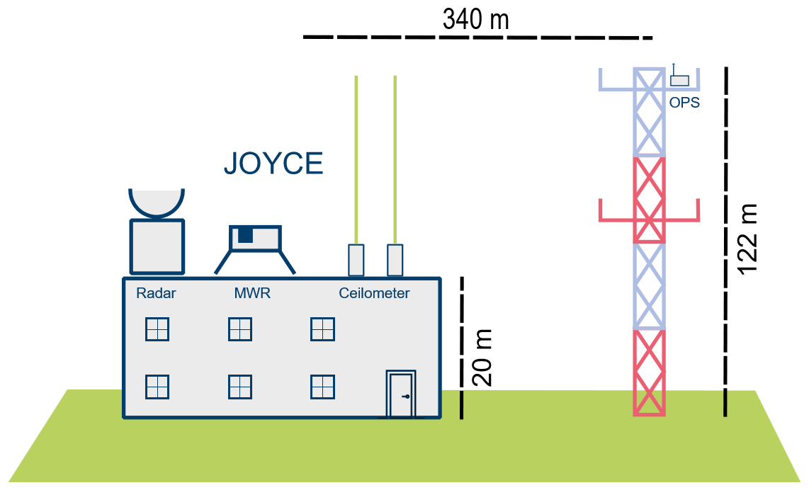
Figure 1 Not true-to-scale schematic of the experimental setup showing distances of the meteorological tower hosting the optical particle sizer (OPS) to JOYCE with two ceilometers, a cloud radar and a microwave radiometer (MWR) at Forschungszentrum Jülich.

JOYCE is equipped with a suite of remote sensing, in situ and radiation measurement instruments. The instrumentation comprises a Metek MIRA-36 Doppler cloud radar, two ceilometers (Vaisala CT25k and Lufft CHM15k; Sect. 3.1), an RPG humidity and temperature profiler, and a CIMEL sun photometer. In this study, only the ceilometer measurements are analyzed using the sun photometer to estimate the lidar ratio (Sect. 4.2), while the remaining instruments provide input for the Cloudnet target classification (Sect. 3.3). The JOYCE data repository offers 16 years of ceilometer data. Additionally, a 120 m meteorological tower is located closeby. This tower provides standard meteorological measurements at seven platforms (10, 20, 30, 50, 80, 100 and 120 m). The tower has a horizontal distance of 340 m from the JOYCE site. For this study, the tower was equipped with an optical particle sizer (OPS) (TSI OPS 3330) as an in situ instrument for comparison with the ceilometer aerosol retrievals. A scheme of the setup is shown in Fig. 1.

3 Instrumentation

3.1 Ceilometers

Ceilometers are basic near-infrared lidar systems. They emit eye-safe laser pulses with a high frequency. The pulses are then scattered back to the instrument by cloud droplets, aerosols and gas-phase constituents. From the run-time, the distance to the scattering target is estimated. The intensity of the scattered signal can be used to determine the optical properties of the scattering target. The measured power P at the ceilometer receiver as a function of range r and time t can be described by the following equation (Klett, 1981; Hervo et al., 2016):

$$\begin{array}{}\text{(1)}& P(r,t)={\displaystyle \frac{\mathrm{1}}{r^{\mathrm{2}}}}{C}_{\mathrm{L}}\left(t\right)O(r,t)\mathit{\beta }(r,t)e^{-\mathrm{2}{\int }_{\mathrm{0}}^r\mathit{\sigma }(r^{\prime },t)\mathrm{d}{r}^{\prime }}+B\left(t\right)\end{array}$$

Here C_L represents a calibration factor (also known as lidar-constant), which contains device-specific parameters. The signal is also dependent on the overlap function O(r,t), the extinction coefficient σ, the backscatter coefficient β and a solar background signal B(t). It is common to define the range corrected signal (RCS) as:

$$\begin{array}{}\text{(2)}& \mathrm{RCS}=\left(P\right(r,t)-B(t\left)\right)r^{\mathrm{2}}\end{array}$$

Each ceilometer generates manufacturer-dependent raw data that were brought to unified L1 data by the E-Profile algorithm Raw2L1 (Haefele et al., 2016).

JOYCE is equipped with two ceilometers (Table 1) representing the two main types of ceilometers, namely monoaxial (CT25k) and biaxial (CHM15k) setups. Monoaxial systems use a single light path for emitting and receiving the laser pulses and a semi-transparent mirror to split the beam. In contrast, biaxial ceilometers use two separate light paths. The downside of this approach is a range with incomplete overlap, which affects measurements of the CHM15k in the lowest about 350 m (Schween et al., 2014). This problem is significantly reduced for the Vaisala CT25k, which covers the lowest range gate but has a significantly lower pulse energy. Based on an internal overlap correction, measurements are usable starting at 0 m (Münkel et al., 2006). However, hardware and software related artefacts were reported for measurements below 70 m for a comparable ceilometer (Vaisala CL31) (Kotthaus et al., 2016). The Lufft CHM15k uses an avalanche photon detector (APD) in photon-counting mode, which allows higher SNR at high altitudes, compared to photocurrent method instruments like the Vaisala CT25k (Markowicz et al., 2008; Schween et al., 2014). It should also be noted that the CT25k and the CHM15k by now have been operational since 16 years and 12 years, respectively, which may have lowered their sensitivity. More advanced, modern ceilometers can produce data of higher quality. However, the intention of this work is to utilize the existing long-term dataset, which requires a characterization of the available instruments. The comparison with the in situ tower measurements will be confined to the CT25k data because of the overlap issue of the CHM15k at 120 m.

Table 1 Ceilometers at JOYCE (based on manufacturer information).

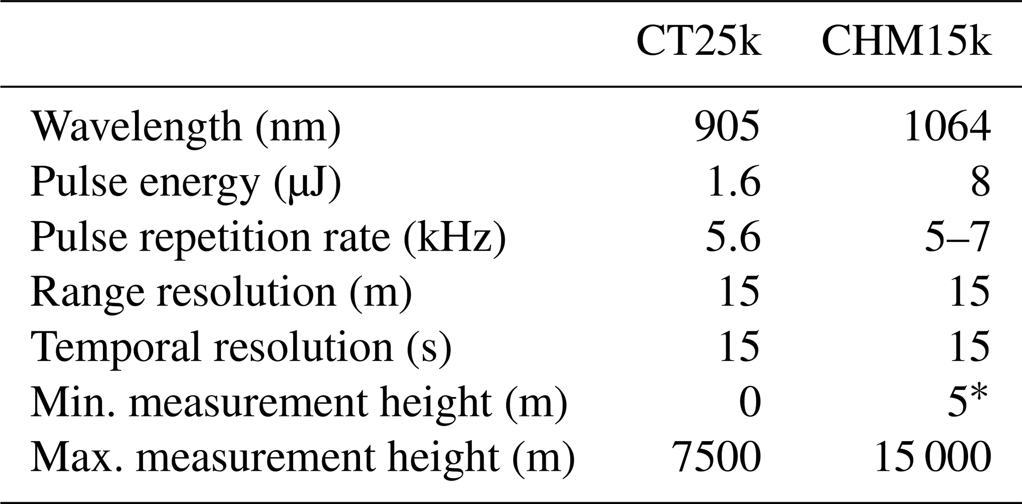
^∗ Reliable aerosol information starting around 350 m, due to limited overlap at lower altitudes (Schween et al., 2014).

3.2 Optical Particle Sizer

To evaluate the ceilometer aerosol-retrieval, a comparison setup was created as shown in Fig. 1 using the meteorological tower with an OPS for in situ measurements of aerosols installed at 120 m above ground. At this altitude, a representative measurement can be made undisturbed by any small-scale influence from the ground or nearby buildings.

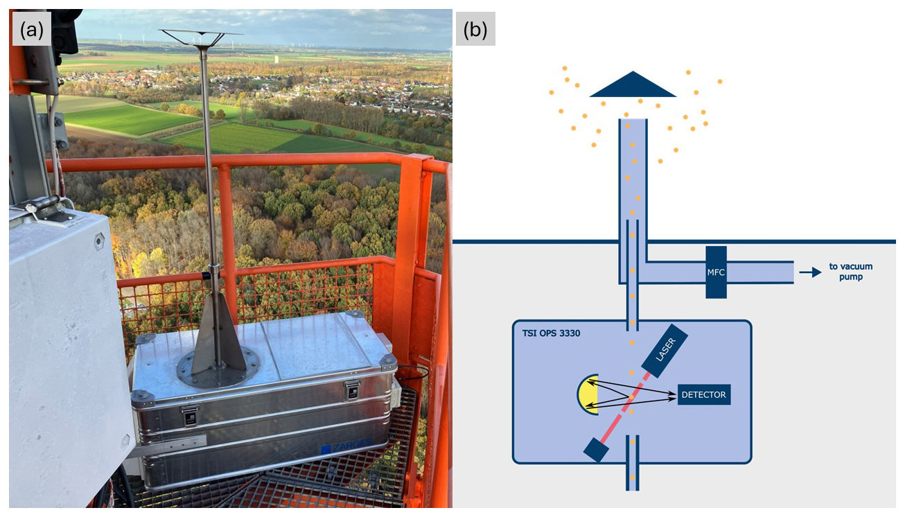
Figure 2 (a) Photograph of the in situ aerosol tower measurement setup at 120 m. (b) Schematic of the instrument consisting of a rain-protected inlet with sampling line, a pump-driven mass flow controller (MFC) and a TSI OPS 3300 for optical particle detection.

The instrument consists of an inlet connected to the OPS in a water-tight box allowing for an omnidirectional aerosol sampling and rain protection (Eckert, 2013). A photograph of the setup is shown in Fig. 2a. The airflow through the inlet of about 15 standard liter per minute (slm) was driven by a pump and controlled by a mass flow controller (MFC). Inside the laminar airflow about 1 slm of air was taken by the OPS instrument. The airflow of the MFC was regulated in a way that an isokinetic sampling by the OPS from the main airflow was obtained (assuming laminar flow conditions). The air was not dried actively. A schematic of the sampling and OPS setup is illustrated in Fig. 2b. Specifications of the OPS can be found in Table 2.

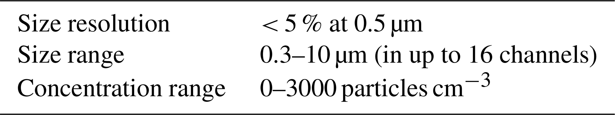
Table 2 Manufacturer specifications of the optical particle sizer TSI OPS 3330.

The instrument works on the principle of light scattering as illustrated in Fig. 2. The inlet air flow (1 L min⁻¹) is focused by a sheath air stream and goes through a light trap where a continuous laser beam (660 nm) passes the particle stream. Scattered light from a range of scattering angles is focused on a photodetector by a mirror. Light scattered by single aerosol particels is registered and assigned to a particle size dependent on the scattered light intensity.

The system allows the measurement of aerosol mass and number concentrations, sorted in 16 user-defined size channels, based on their scattering intensity. According to the manufacturer, data are processed as follows. For each channel, the number concentration C_n in a bin is determined. Based on the number concentration, a mass concentration C_m can be estimated:

$$\begin{array}{}\text{(3)}& C_m=C_n\mathit{\rho }{\displaystyle \frac{\mathit{\pi }{D}_{\mathrm{pv}}^{\mathrm{3}}}{\mathrm{6}}}\end{array}$$

ρ is the particle density (typically in the range 1.2 to 2.5 g cm⁻³; Osborne, 2024) taken as 1.5 g cm⁻³ and D_pv is an effective particle diameter, which is calculated from the bin upper boundary (D_U) and bin lower boundary (D_L):

$$\begin{array}{}\text{(4)}& D_{\mathrm{pv}}=D_{\mathrm{L}}{\left[{\displaystyle \frac{\mathrm{1}}{\mathrm{4}}}\left(\mathrm{1}+{\left({\displaystyle \frac{D_{\mathrm{U}}}{D_{\mathrm{L}}}}\right)}^{\mathrm{2}}\right)\left(\mathrm{1}+\left({\displaystyle \frac{D_{\mathrm{U}}}{D_{\mathrm{L}}}}\right)\right)\right]}^{\frac{\mathrm{1}}{\mathrm{3}}}\end{array}$$

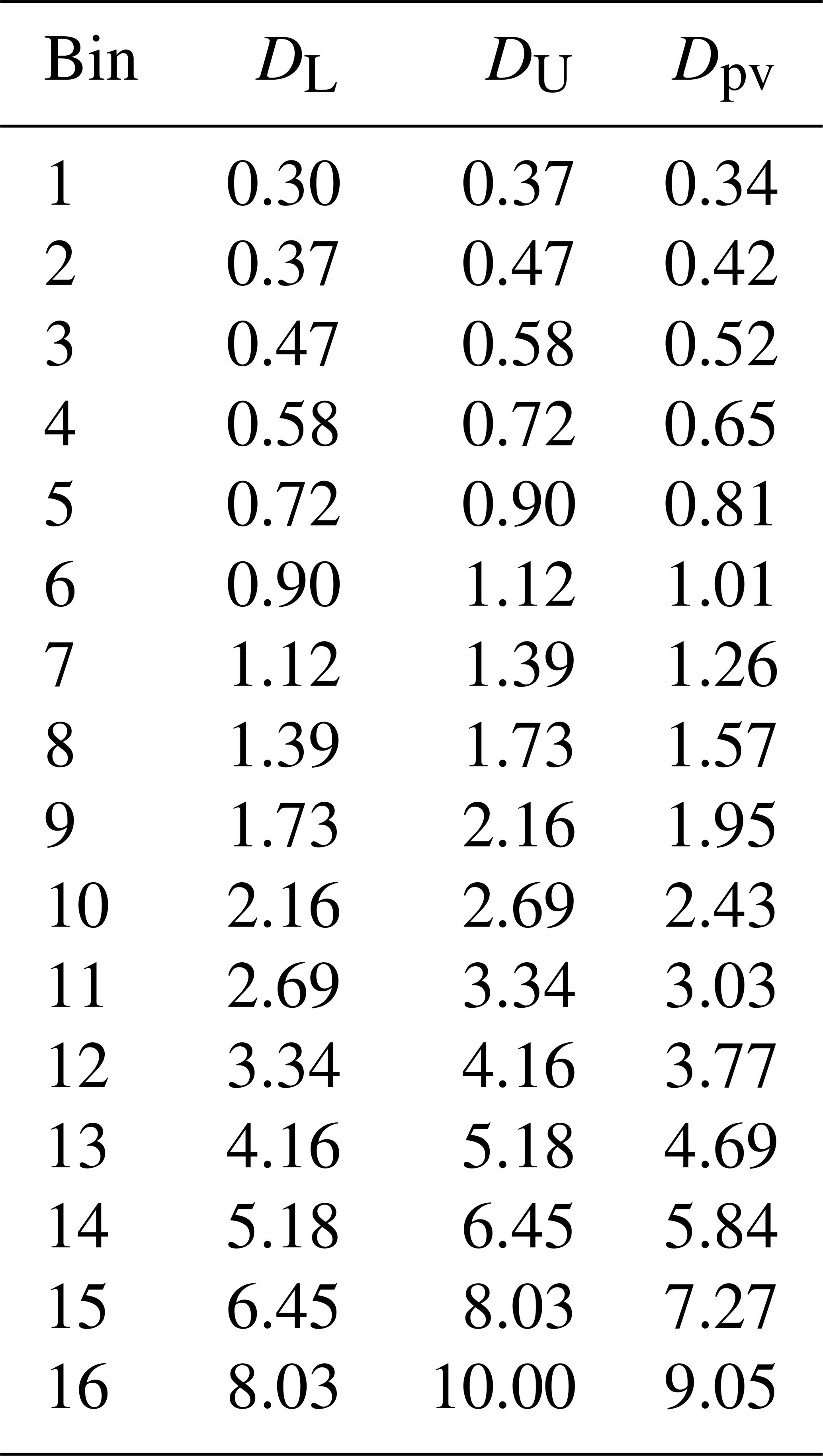
Size bins were selected based on a predefined protocol (TSI Default) as summarised in Table A1 in the appendix to cover the full size range the instrument provides (0.3–10 µm). Moreover, a temporal resolution of 5 min and a sample time of 1 min were selected for the measurements.

3.3 Cloudnet

The Cloudnet target classification (Hogan and O'Connor, 2004) is utilized to characterize the atmospheric boundary layer regarding the presence of aerosols, insects, clouds and precipitation. Cloudnet was founded to combine ground based cloud remote sensing instruments to a network and to generate synergistic products (Illingworth et al., 2007). The minimum instrumentation consists of a Doppler cloud radar, a ceilometer and a dual-frequency microwave radiometer. Today, Cloudnet is integrated into the center for cloud remote sensing (CCRES) within ACTRIS (Pappalardo, 2018; Laj et al., 2024). Currently there are 29 contributing sites registered (Cloudnet, 2025). The Cloudnet target classification combines radar reflectivity, ceilometer backscatter, model parameters, microwave radiometer LWP measurements and rain gauge measurements into a single classification product. For each height layer, the bit values can be set for presence of small liquid droplets, presence of falling hydrometeors, wet-bulb temperature below 0 °C, presence of melting ice particles, presence of aerosols and presence of insects. At JOYCE, the Cloudnet target classification, which utilises the Lufft CHM15k ceilometer, is available on a grid of 36 m vertical resolution and 30 s temporal resolution. In the following, it will be used to filter out conditions where remote aerosol detection by the ceilometers may be adversely affected by liquid clouds, ice clouds or precipitation.

4 Ceilometer Aerosol Retrieval

4.1 Calibration Verification

To use the RCS of a ceilometer for aerosol measurements, a calibration of the signal is necessary. The goal of this calibration is to determine the lidar constant C_L to convert the RCS (Eq. 2) into an attenuated backscatter coefficient β_att.

$$\begin{array}{}\text{(5)}& {\mathit{\beta }}_{\mathrm{att}}={\displaystyle \frac{\mathrm{RCS}}{C_{\mathrm{L}}}}\end{array}$$

The commonly used Rayleigh calibration (Wiegner and Geiß, 2012) could not be applied to the Vaisala CT25k ceilometer due to the low signal-to-noise ratio (SNR) in high altitudes for this instrument. In recent years, an additional method was established. The liquid cloud calibration (Hopkin et al., 2019; O'Connor et al., 2004) uses the attenuation of the ceilometer signal in liquid clouds. The lidar ratio S, defined as the ratio of the extinction-to-backscatter coefficient is assumed to be constant inside liquid clouds with a value of S≈18 sr (Pinnick et al., 1983; O'Connor et al., 2004). For cases where the ceilometer signal is fully attenuated by a liquid cloud, the total path integrated attenuated backscatter B can be described as a function of the observed attenuated backscatter coefficient β_att, the height above ground z, the range corrected signal RCS, the multiple-scattering correction η, the lidar ratio and a calibration coefficient C (Hopkin et al., 2019):

$$\begin{array}{}\text{(6)}& B=\underset{\mathrm{0}}{\overset{\mathrm{\infty }}{\int }}{\mathit{\beta }}_{\mathrm{att}}\mathrm{d}z=\underset{\mathrm{0}}{\overset{\mathrm{\infty }}{\int }}C\mathrm{RCS}\mathrm{d}z={\displaystyle \frac{\mathrm{1}}{\mathrm{2}\mathit{\eta }S}}\end{array}$$

In the algorithm, the calibration coefficient C is varied until Bη = 0.0266 m⁻¹. This value represents liquid cloud droplets with S = 18.8 sr (Hopkin et al., 2019). Only profiles with a negligible aerosol backscatter contribution (< 5 %) below the cloud are considered. The optimised calibration coefficient C is the reciprocal of the lidar constant C_L. This method does not require high SNR values in high tropospheric regions and so it can be applied also to avalanche photon detectors in photocurrent detection mode like the Vaisala CT25k.

The JOYCE CT25k already performs an internal calibration, which was verified by the liquid cloud calibration (Hopkin et al., 2019), based on the program code of E-Profile (Haefele et al., 2016). A lidar constant of $C_{\mathrm{L}}=\mathrm{0.97}\pm \mathrm{0.06}$ was determined in the years 2023 and 2024, confirming the internal calibration of the instrument. The manufacturer does not disclose the nature of the internal calibration.

4.2 Aerosol Extinction Profiles

To derive extinction profiles from the ceilometer attenuated backscatter signal the Klett-Fernald-Sasano method (Klett, 1981, 1985) is mostly used where a backward inversion approach is applied to solve the lidar equation. The calculations start in the high, aerosol-free part of the atmosphere (Rayleigh-atmosphere) and iteratively derive the extinction coefficients.

To use the Klett-Fernald-Sasano approach, a high SNR in high layers is necessary. This requirement can not be fulfilled when using a Vaisala CT25k ceilometer. For this reason, a forward method was used (Li et al., 2021). For each layer z_i, starting at the ground with initial conditions based on the β_att, the aerosol transmittance T_a, the molecular transmittance T_m, the aerosol backscatter coefficient β_a and the molecular backscatter coefficient β_m are calculated in an iterative process (k = 1, 2, 3 …). The values of T_m(z_i) and β_m(z_i) were calculated from the station altitude based on an algorithm-specific Rayleigh atmosphere. Here τ_a represents the aerosol optical depth and σ_a the aerosol extinction coefficient.

$$\begin{array}{}\text{(7)}& {\displaystyle }{\mathit{\tau }}_{\mathrm{a}}(z_i,k)={\mathit{\tau }}_{\mathrm{a}}\left(z_{i-\mathrm{1}}\right)+{\mathit{\sigma }}_{\mathrm{a}}(z_i,k-\mathrm{1})\cdot \mathrm{\Delta }{z}_i\text{(8)}& {\displaystyle }{T}_{\mathrm{a}}^{\mathrm{2}}(z_i,k)=e^{-\mathrm{2}{\mathit{\tau }}_{\mathrm{a}}(z_i,k)}\text{(9)}& {\displaystyle }{\mathit{\beta }}_{\mathrm{a}}(z_i,k)={\displaystyle \frac{{\mathit{\beta }}_{\mathrm{att}}\left(z_i\right)}{T_{\mathrm{m}}^{\mathrm{2}}\left(z_i\right)\cdot T_{\mathrm{a}}^{\mathrm{2}}(z_i,k)}}-{\mathit{\beta }}_{\mathrm{m}}\left(z_i\right)\end{array}$$

At every iteration step k, the extinction coefficient σ_a is calculated with the lidar ratio S_a:

$$\begin{array}{}\text{(10)}& {\mathit{\sigma }}_{\mathrm{a}}(z_i,k)=S_{\mathrm{a}}\cdot {\mathit{\beta }}_{\mathrm{a}}(z_i,k)\end{array}$$

The iterative process is stopped if either 30 iteration steps are reached or if the relative change of the extinction coefficient σ_a is smaller than 0.01 %. Then the current value of σ_a, τ_a and β_a are set and the process starts for the next layer. This method was implemented in the Python-library A-Profiles (Mortier, 2022). For this study, we used this forward inversion algorithm for the Vaisala CT25k ceilometer.

The lidar ratio $S_{\mathrm{a}}={\mathit{\sigma }}_{\mathrm{a}}/{\mathit{\beta }}_{\mathrm{a}}$ is unknown for ceilometer measurements. Therefore, it was estimated based on a multi-year mean value of $S_{\mathrm{a}}=(\mathrm{47}\pm \mathrm{13})$ sr for a wavelength of 1020 nm from the AERONET (AErosol RObotic NETwork; Holben et al., 1998) inversion product of a CIMEL sun photometer installed next to the ceilometers. The uncertainty of S_a is a major contributor to the overall uncertainty of retrieving σ_a from a ceilometer with this method.

4.3 Calculation of aerosol mass concentration

Aerosol mass concentration C_m can be calculated from the aerosol extinction coefficient σ_a by an extinction to mass coefficient (EMC):

$$\begin{array}{}\text{(11)}& C_m={\displaystyle \frac{{\mathit{\sigma }}_{\mathrm{a}}}{\mathrm{EMC}}}\end{array}$$

The EMC is dependent on the aerosol type, size distribution and the ceilometer wavelength. The EMC can either be predicted theoretically by Mie simulations (Mortier, 2022) or determined based on in situ C_m and ceilometer-derived σ_a. A discussion of the experimental EMC values found in this study compared to literature values can be found in Sect. 5.3.

5 Results and Discussion

The results section is split into five subsections. At first, an overview of the in situ and ceilometer datasets is given and data from an example day are presented. Afterwards, the quality of retrieving aerosol mass concentrations from ceilometer backscatter coefficients and ceilometer aerosol extinction coefficients is evaluated. Finally, an attempt is presented to reproduce aerosol backscatter and extinction coefficients based on the measured size distributions, followed by a critical assessment of the OPS measurements.

5.1 Dataset overview and example day

A dataset of ceilometer-derived attenuated backscatter coefficients in 120 m and of in situ aerosol mass concentrations in the same height was acquired for the period 1 February to 20 June 2023. There was a 10 d interruption from 22 February to 3 March because of a blocked exhaust filter and a 7 d interruption from 4 to 12 April caused by an outage in ceilometer measurements. The dataset was screened to avoid contamination by hydrometeors in the ceilometer signal, based on the Cloudnet target classification (Sect. 3.3). To further refine this selection, data were discarded when the relative humidity (RH) measured at 120 m exceeded 95 % and cloud radar reflectivity at the lowest possible measurement height (255 m) was above −20 dBZ at 35 GHz.

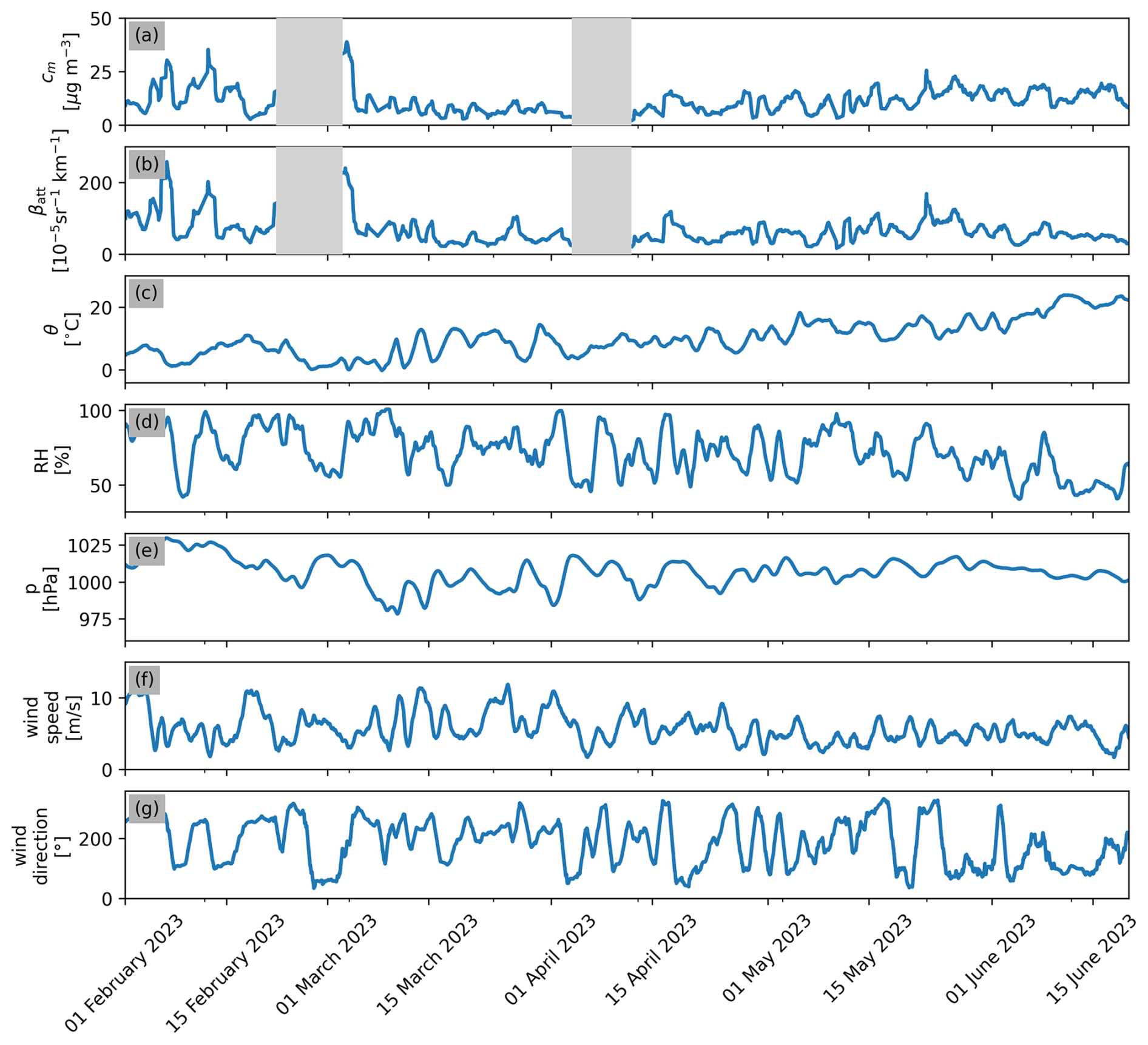
Figure 3 Atmospheric conditions during the measurement period from 1 February to 20 June 2023 with (a) OPS in situ aerosol mass concentration C_m at 120 m, (b) ceilometer attenuated backscatter signal β_att at 120 m and further in situ data: (c) temperature θ at 120 m, (d) humidity RH at 120 m, (e) ground air pressure p at 2 m, (f) wind speed at 120 m, and (g) wind direction at 50 m. All data are shown as 1 d rolling means. C_m and β_att were filtered based on the criteria specified in Sect. 5.1.

Figure 3 provides an overview of the dataset, including additional measurements from the meteorological tower. The mean aerosol mass concentration during the observation period was C_m = 11.5 µg m⁻³. The mean temperature and relative humidity were θ = (12 ± 7) °C and RH = (76 ± 19) %, respectively. The wind speed at 120 m above ground on average was (6 ± 3) m s⁻¹. For the measurement period, no coherent wind direction measurement in 120 m was available. For this reason, the wind direction at the meteorological tower 50 m above ground is shown in Fig. 3. The predominant wind direction at 50 m was west-southwest.

To illustrate typical diurnal changes in aerosol concentration, 14 February 2023 was selected as an example. This day was dominated by a high-pressure ridge over Central Europe. The ridge went along with a surface high-pressure system. This situation creates stable conditions with no clouds or precipitation over the day.

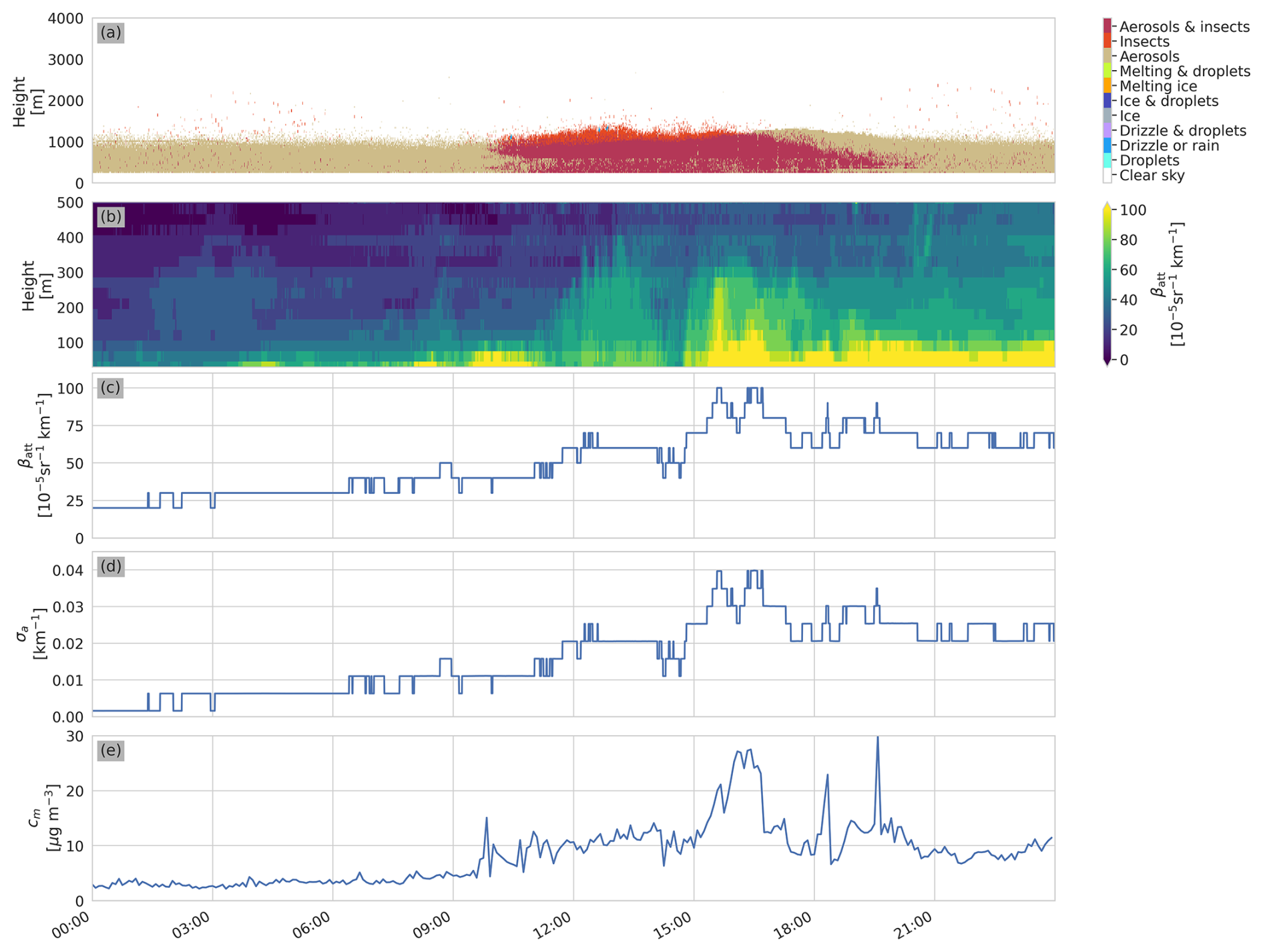
Figure 4 One day case study from 14 February 2023 in Jülich, showing (a) the Cloudnet target classifications, (b) ceilometer attenuated backscatter coefficients β_att, (c) ceilometer attenuated backscatter coefficients β_att at 120 m, (d) ceilometer-derived aerosol extinction coefficients σ_a at 120 m and (e) in situ aerosol mass concentration C_m at 120 m. Times are given in UTC.

As shown in Fig. 4a, the Cloudnet target classification confirmed no clouds or precipitation in the boundary layer while aerosols were present for the whole day. These conditions make that day ideal for comparing the ceilometer aerosol retrieval with the in situ observation. In the time range from 00:00 to about 09:00 UTC low aerosol mass concentrations of C_m < 5 µg m⁻³ are visible in the tower observations (Fig. 4e). This goes along with low ceilometer backscatter coefficients of ${\mathit{\beta }}_{\mathrm{att}}<\mathrm{40}\times {\mathrm{10}}^{-\mathrm{5}}$ sr⁻¹ km⁻¹ (Fig. 4c). The vertical extent of the aerosol layer below 250 m is visible in the ceilometer backscatter profiles (Fig. 4b). With the development of the mixing layer after 09:00 UTC, the aerosol mass concentration increased up to C_m = 30 µg m⁻³. This trend is also visible in the ceilometer-derived aerosol extinction coefficients (Fig. 4d) and in the ceilometer backscatter coefficients, which increased up to β_att = $\mathrm{100}\times {\mathrm{10}}^{-\mathrm{5}}$ sr⁻¹ km⁻¹ (Fig. 4c).

This example demonstrates qualitativly that ceilometer backscatter coefficients can reproduce the overall change in aerosol concentration. Steplike levels of ceilometer backscatter coefficients can be explained by the low signal resolution of the Vaisala CT25k (Sect. 3.1).

5.2 Aerosol mass concentration and attenuated backscatter coefficient

In the next step, we now statistically relate measured attenuated backscatter coefficients β_att to in situ measured aerosol mass concentrations C_m.

For the following analyses, a combined dataset based on OPS-measurement, ceilometer, and Cloudnet data was generated. All data were mapped on the 5 min time grid of the OPS-measurements based on a nearest neighbour approach, resulting in a total of 5443 data points after applying the filtering criteria (Sect. 5.1). Figure 5 indicates a linear correlation between ceilometer attenuated backscatter coefficient β_att and in situ aerosol mass concentration C_m with a Pearson correlation coefficient R = 0.73. This result is in reasonable agreement with a previous study by Münkel et al. (2006) who obtained a correlation coefficient of R = 0.84 between ground-level PM₁₀ aerosol mass concentration and the attenuated backscatter coefficient of a co-located CT25k in an urban environment.

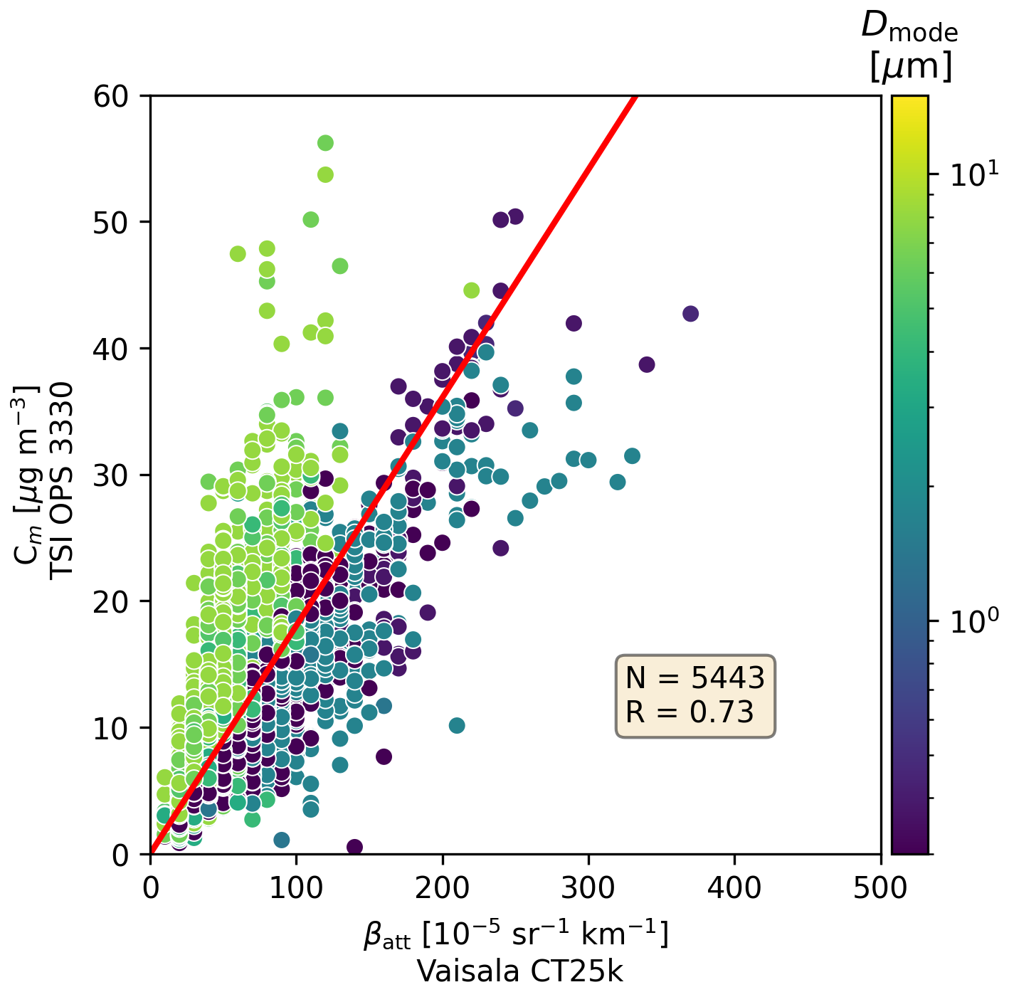
Figure 5 Comparison of ceilometer attenuated backscatter coefficients β_att in 120 m and total in situ aerosol mass concentration C_m (1 February–20 June 2023). The inset indicates the number of data points N and the correlation coefficient R. The full red line shows the result of a linear regression (Eq. 12). Data points were color-coded according to the diameter D_mode of the size bin with the maximum aerosol mass concentration.

To derive an empirical relationship between attenuated backscatter coefficients and total aerosol mass concentrations, a least squares linear regression was derived resulting in the following expression for a ceilometer-derived aerosol mass concentration $C_m^{\mathit{\beta }}$:

$$\begin{array}{}\text{(12)}& {\displaystyle \frac{C_m^{\mathit{\beta }}}{\mathrm{\mu }\mathrm{g}{\mathrm{m}}^{-\mathrm{3}}}}=\mathrm{0.18}\cdot {\displaystyle \frac{{\mathit{\beta }}_{\mathrm{att}}}{{\mathrm{10}}^{-\mathrm{5}}{\mathrm{sr}}^{-\mathrm{1}}{\mathrm{km}}^{-\mathrm{1}}}}\end{array}$$

Neglecting the small contribution of molecular backscatter that is discussed in Sect. 5.3, the line was forced through the origin. The corresponding regression line is shown in Fig. 5. Its slope is again in reasonable agreement with the result by Münkel et al. (2006) who derived a value of 0.20 × 10⁵ µg m⁻³ sr km and a small offset of −1.6 µg m⁻³.

To estimate the uncertainty of deriving aerosol mass concentration from β_att, a mean absolute percentage error (MAPE) was calculated considering all N data points:

$$\begin{array}{}\text{(13)}& \mathrm{\Delta }{C}_m^{\mathit{\beta }}={\displaystyle \frac{\mathrm{1}}{N}}\sum _{i=\mathrm{1}}^N\left|{\displaystyle \frac{C_{m,i}^{\mathit{\beta }}-C_{m,i}}{C_{m,i}}}\right|\times \mathrm{100}\mathit{\%}=\mathrm{31}\mathit{\%}\end{array}$$

The corresponding RMSE is 4.7 µg m⁻³. As is evident from Fig. 5 the scatter is significant and can be explained by instrumental uncertainties, varying aerosol optical properties, aerosol composition, particle size, and particle shape. The color-coding based on the diameter D_mode of the OPS size bin with the maximum aerosol mass concentration implies a dependence of the relationship on the particle size distribution that is addressed in Sect. 5.4.

This analysis demonstrates that ceilometer β_att measurements are, in principle, suitable for obtaining information on aerosol mass concentration. However, the statistical relation obtained here is valid only for the site- and instrument-specific set-up. Additionally, they represent only measurements during defined environmental conditions, as described above, from a five-month dataset.

5.3 Aerosol mass concentration and extinction coefficient

In this section we now analyse the relation of the in situ measured aerosol mass concentrations to the aerosol extinction coefficients, derived from β_att. Any influence of molecular backscatter that is included in β_att should be eliminated in the retrieval of aerosol extinction coefficients. Ceilometer-derived σ_a were calculated from the ceilometer attenuated backscatter coefficient β_att by the forward inversion method described in Sect. 4.2 (Li et al., 2021). Figure 6 shows the obtained σ_a as a function of the corresponding β_att revealing a compact linear relationship with a correlation coefficient close to unity. A linear regression results in:

$$\begin{array}{}\text{(14)}& {\displaystyle \frac{{\mathit{\sigma }}_{\mathrm{a}}}{{\mathrm{km}}^{-\mathrm{1}}}}=-\mathrm{0.008}+\mathrm{47.6}\cdot {\displaystyle \frac{{\mathit{\beta }}_{\mathrm{att}}}{{\mathrm{sr}}^{-\mathrm{1}}{\mathrm{km}}^{-\mathrm{1}}}}\end{array}$$

The slope of 47.6 sr closely resembles the a priori lidar ratio of S_a=47 sr that was applied (Sect. 4.2) with a y-intercept of (−0.008 ± 0.002) km⁻¹. This intercept corresponds to the influence of molecular backscatter that is included in β_att and should be eliminated in the retrieval of σ_a. The intercept value can be converted to a pure air backscattering coefficient of about (1.7 ± 0.4) × 10⁻⁴ sr⁻¹km⁻¹. Taking the theoretical Rayleigh scattering lidar ratio of $\mathrm{8}\mathit{\pi }/\mathrm{3}$ sr, an extinction coefficient of (1.4 ± 0.4) × 10⁻³ km⁻¹ at 120 m was obtained. This estimate is in reasonable agreement with a value of (1.50±0.04) × 10⁻³ km⁻¹ for 906 nm derived from the literature for the measurement conditions (Bucholtz, 1995). In contrast, a comparison of the vertically integrated σ_a with AERONET aerosol-optical-depths (AOD) shows a significant underestimation. This can be explained by the low SNR of the CT25k at higher altitudes (Markowicz et al., 2008) leading to an underestimation of the derived σ_a. The comparison is provided in Sect. B of the Appendix.

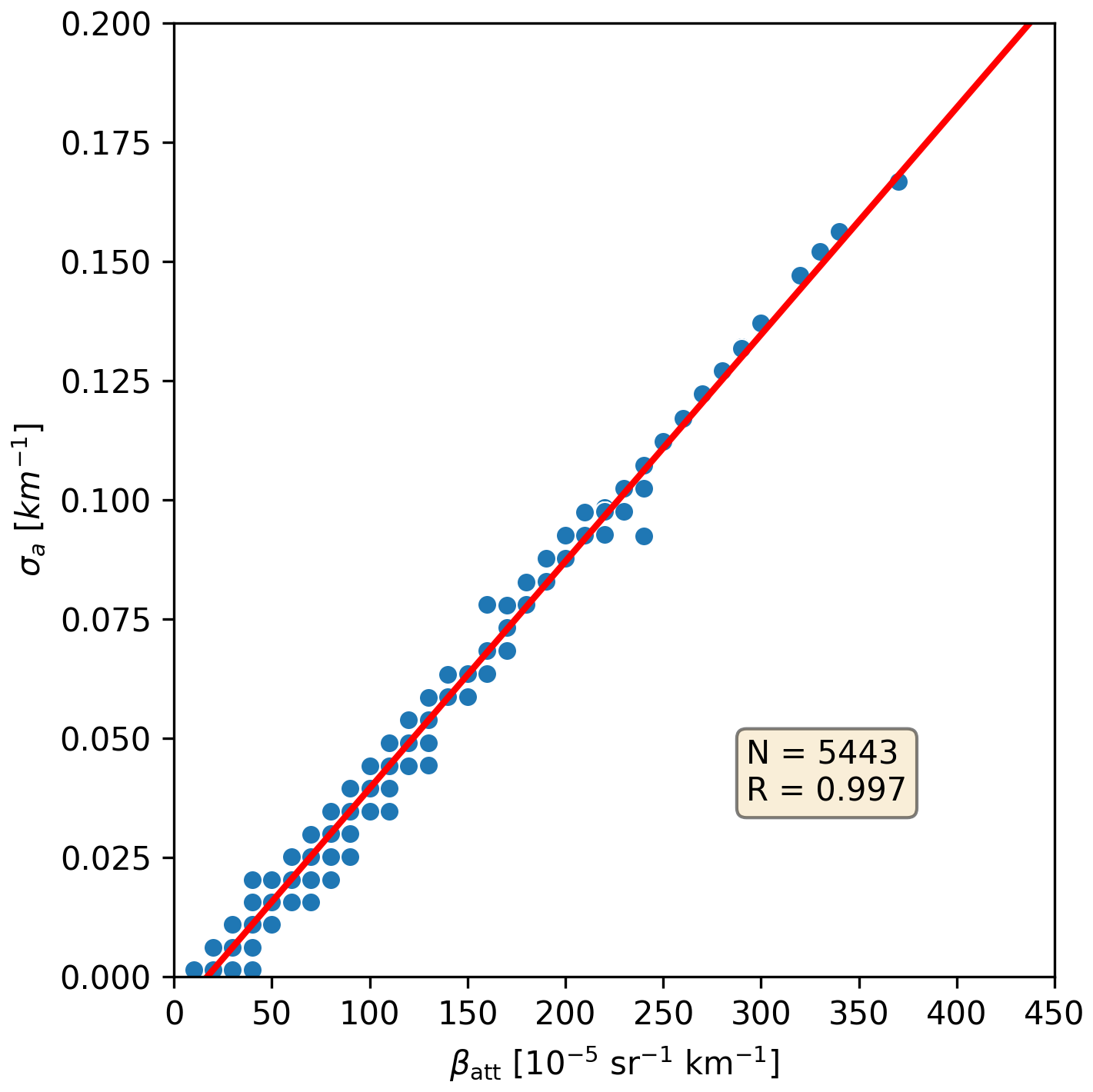
Figure 6 Comparison of ceilometer attenuated backscatter coefficients β_att in 120 m and corresponding aerosol extinction coefficients σ_a, derived by a forward inversion method (1 February–20 June 2023) according to Li et al. (2021). The inset indicates the number of data points N and the correlation coefficient R. The red line corresponds to the regression line (Eq. 14).

Because of the strong correlation between β_att and σ_a, a plot of C_m as a function of σ_a exhibits virtually the same scatter as C_m as a function of β_att (Fig. 5) with a similar Pearson correlation coefficient of R = 0.73. The corresponding plot is shown in Fig. 7.

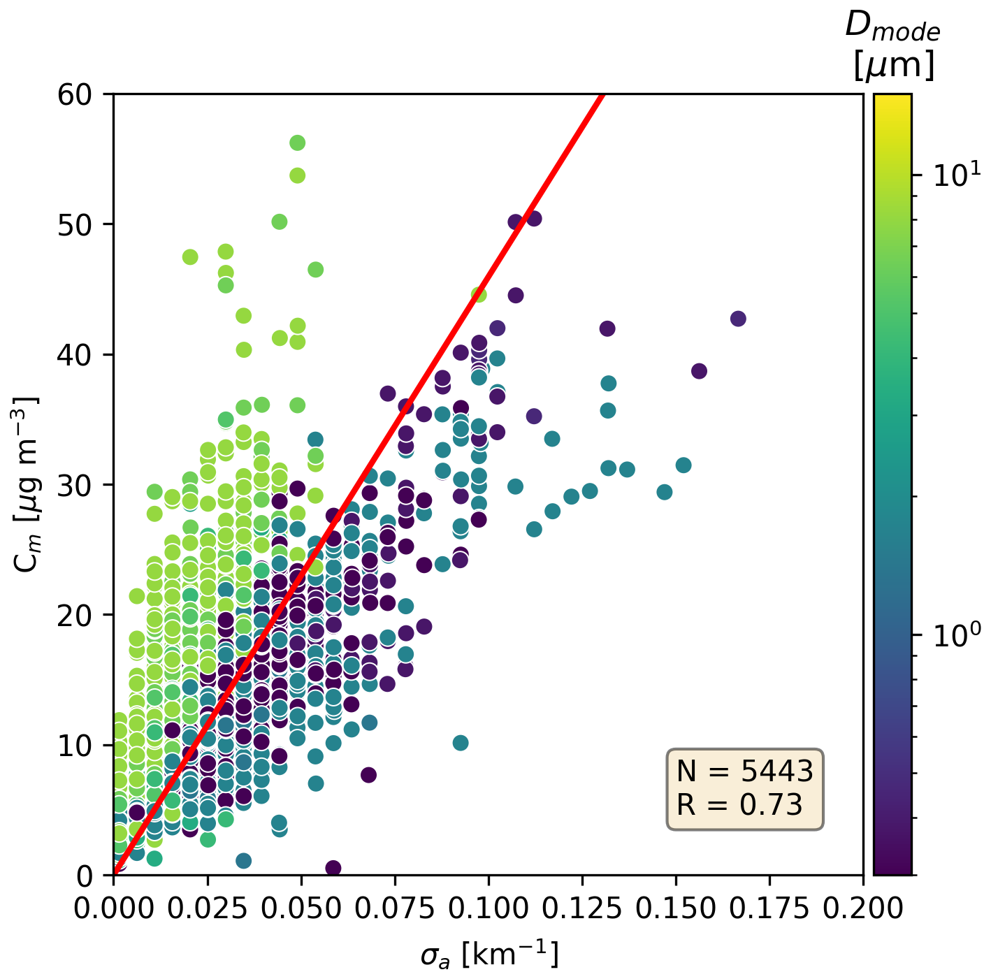
Figure 7 Comparison of ceilometer-derived aerosol extinction coefficients σ_a in 120 m and total in situ aerosol mass concentration C_m (1 February–20 June 2023). The inset indicates the number of data points N and the correlation coefficient R. The full red line shows the result of a linear regression (Eq. 15). Data points were color-coded according to the diameter D_mode of the size bin with the maximum aerosol mass concentration.

A linear regression through the origin between C_m and σ_a results in an empirical relation for an extinction-derived aerosol mass concentration $C_m^{\mathit{\sigma }}$:

$$\begin{array}{}\text{(15)}& {\displaystyle \frac{C_m^{\mathit{\sigma }}}{\mathrm{\mu }\mathrm{g}{\mathrm{m}}^{-\mathrm{3}}}}=\mathrm{460}\cdot {\displaystyle \frac{{\mathit{\sigma }}_{\mathrm{a}}}{{\mathrm{km}}^{-\mathrm{1}}}}\end{array}$$

Consistently, no improvement in the relative uncertainty of deriving aerosol mass concentration from σ_a was achieved, i.e. $\mathrm{\Delta }{C}_m^{\mathit{\sigma }}$ = 39 % (RSME = 5.7 µg m⁻³), compared to $\mathrm{\Delta }{C}_m^{\mathit{\beta }}$ = 31 %. However, knowledge of the true lidar ratio for each measurement is expected to reduce $\mathrm{\Delta }{C}_m^{\mathit{\sigma }}$, making σ_a a better proxy for the aerosol mass concentration. This hypothesis is discussed in the next section.

Equation (15) corresponds to EMC = (2.2 ± 0.9) m² g⁻¹, which is high compared to literature values from ceilometer networks like ALICEnet: EMC = (0.9–1.2) m² g⁻¹ and UK Met Office: EMC = (0.7–1.3) m² g⁻¹ (Osborne, 2024). Part of this difference can be explained by the smaller wavelength of the Vaisala CT25k (906 nm) compared to the Lufft CHM15k (1064 nm) for which the literature values apply. Typical Angström exponents of 1.2 ± 0.5 would result in ratios ${\mathit{\sigma }}_{\mathrm{a},\mathrm{1064}}/{\mathit{\sigma }}_{\mathrm{a},\mathrm{906}}=\mathrm{0.83}\pm \mathrm{0.06}$ shifting the EMC closer to the literature values, i.e. EMC = (1.8 ± 0.7) m² g⁻¹ for a wavelength of 1064 nm. A recent study reported 911 nm extinction-to-volume coefficients of 0.448 Mm µm³ cm⁻³ for continental aerosols (Ansmann et al., 2026), confirming a lower EMC of 1.5 m² g⁻¹ based on a common density of 1.5 g cm⁻³.

5.4 Calculation of aerosol backscatter and extinction coefficients

In this section, we now attempt to explain the discrepancies in the derived EMC to previous literature studies. For this, we simulated β_a and σ_a based on Mie-theory and the measured OPS size distributions. Following an approach by Sundström et al. (2009), particle extinction efficiencies Q_ext for the ceilometer wavelength of λ = 906 nm were calculated (Prahl, 2025) for 1000 spherical aerosol particles with diameters linearly distributed between 0.3 and 10 µm. Refractive indices were varied between m = 1.3−0i (water) and m = 1.7−0i (dolomite), covering a typical range of naturally occurring particle properties (Reid et al., 2003). For each size bin of the OPS (Table A1), the mean of Q_ext was calculated and converted to the aerosol extinction cross section by multiplication with the geometrical cross section $\mathit{\pi }{D}_{\mathrm{pv}}^{\mathrm{2}}/\mathrm{4}$. The total aerosol extinction coefficients ${\mathit{\sigma }}_{\mathrm{a}}^{\mathrm{Mie}}$ for each OPS measurement were then calculated based on the measured aerosol number size distribution. Mean size bin lidar ratios were determined accordingly from the phase functions of the spherical particles. Combined with the extinction coefficients, aerosol backscatter coefficients were obtained for the size bins and finally the ${\mathit{\beta }}_{\mathrm{a}}^{\mathrm{Mie}}$ of the measured size distributions. The different ranges of ${\mathit{\beta }}_{\mathrm{a}}^{\mathrm{Mie}}$ for the different refractive indices are shown in Fig. 8. Lidar ratios $S_{\mathrm{a}}^{\mathrm{Mie}}={\mathit{\sigma }}_{\mathrm{a}}^{\mathrm{Mie}}/{\mathit{\beta }}_{\mathrm{a}}^{\mathrm{Mie}}$ for the size distributions can be defined as well.

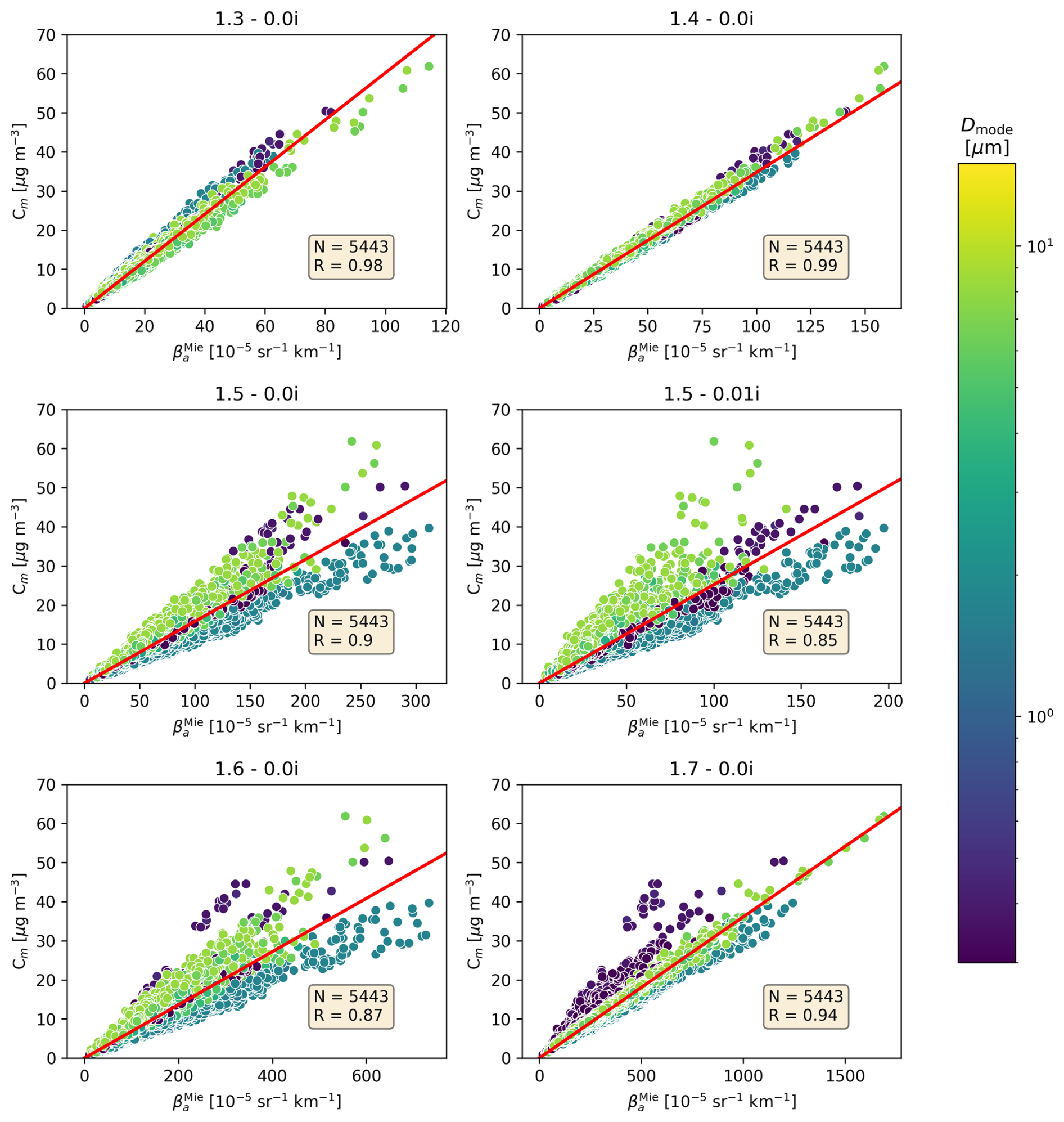
Figure 8 Comparison of simulated aerosol backscatter coefficients ${\mathit{\beta }}_{\mathrm{a}}^{\mathrm{Mie}}$ for different refractive indices, based on in situ aerosol size distributions in 120 m and total in situ aerosol mass concentration C_m (1 February–20 June 2023). The inset indicates the number of data points N and the correlation coefficient R. The full red line shows the result of a linear regression (Table 3). Data points were color-coded according to the diameter D_mode of the size bin with the maximum aerosol mass concentration.

Table 3 Slopes of regression lines (r) and Pearson correlation coefficients (R) of the relationships between simulated aerosol properties based on measured size distributions (${\mathit{\sigma }}_{\mathrm{a}}^{\mathrm{Mie}}$, ${\mathit{\beta }}_{\mathrm{a}}^{\mathrm{Mie}}$), ceilometer-derived extinction coefficients (σ_a) and in situ measured aerosol mass concentration (C_m) as a function of particle refractive index. The last column contains the simulated lidar ratio $S_{\mathrm{a}}^{\mathrm{Mie}}$.

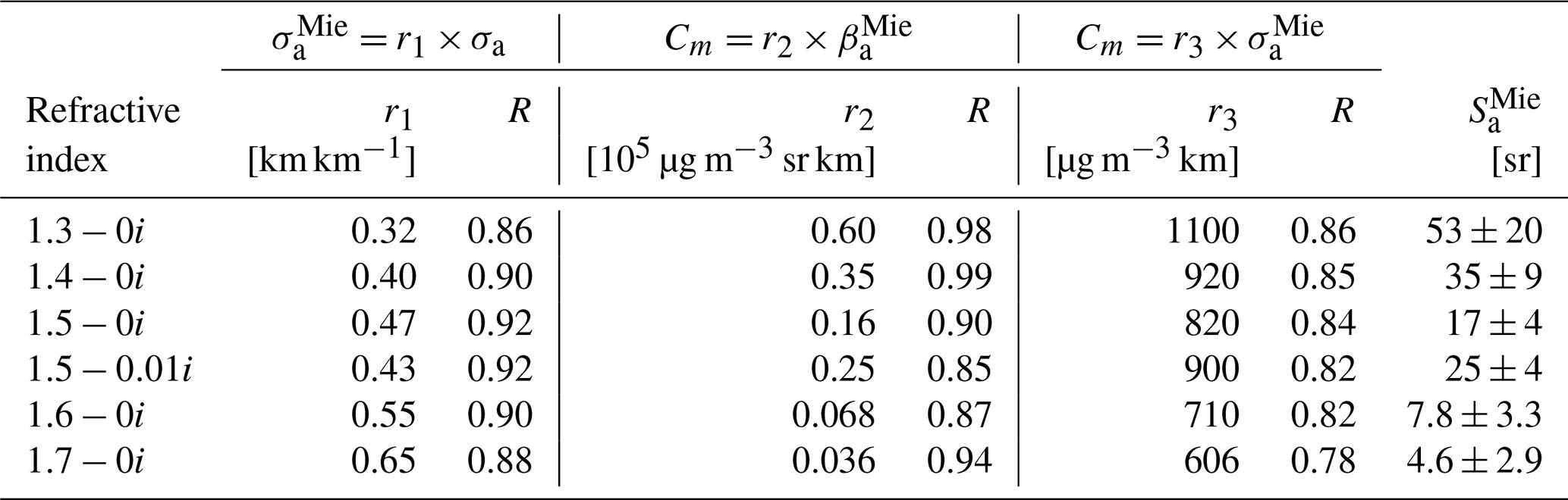
The results of the calculations are summarized in Table 3. Slopes and correlation coefficients of regression lines for different particle refractive indices are listed for C_m as a function of ${\mathit{\sigma }}_{\mathrm{a}}^{\mathrm{Mie}}$ and ${\mathit{\beta }}_{\mathrm{a}}^{\mathrm{Mie}}$, ${\mathit{\sigma }}_{\mathrm{a}}^{\mathrm{Mie}}$ as a function of σ_a, as well as the lidar ratios $S_{\mathrm{a}}^{\mathrm{Mie}}$ for the 5443 size distributions. With one exception, correlation coefficients range above 0.82.

As an example, Fig. 9 shows the dependence of measured C_m as a function of ${\mathit{\sigma }}_{\mathrm{a}}^{\mathrm{Mie}}$ for a refractive index of 1.5, revealing a comparable scatter and color-coding pattern as in Figs. 5 and 7. A plot of calculated and ceilometer-derived extinction coefficients against each other is shown for this example in Fig. 10 and confirms that the D_mode dependence no longer affects the relationship, which is reflected in a greater correlation coefficient of R = 0.92 compared to R = 0.73 in Figs. 5 and 7, and R = 0.84 in Fig. 9. This result can be explained by different particle size dependencies of the aerosol particle mass (∝D³) and scattering cross section (∝D²) which adversely affect the correlations of aerosol mass concentrations and extinction coefficients for the investigated collection of variable size distributions. However, despite the strong correlation in Fig. 10, the ${\mathit{\sigma }}_{\mathrm{a}}^{\mathrm{Mie}}$ and σ_a differ by a factor of about 0.5. Comparable results were obtained for other refractive indices which produce ratios between ${\mathit{\sigma }}_{\mathrm{a}}^{\mathrm{Mie}}$ and σ_a in a reasonably narrow range of 0.49 ± 0.17 (Table 3).

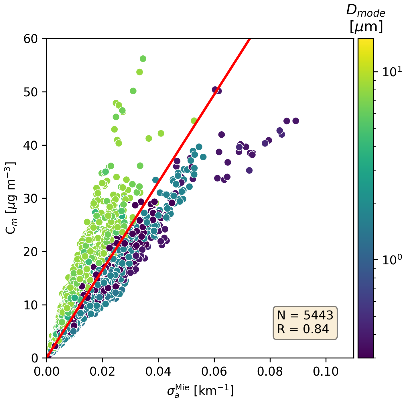
Figure 9 Comparison of simulated aerosol extinction coefficients ${\mathit{\sigma }}_{\mathrm{a}}^{\mathrm{Mie}}$ for a refractive index of 1.5, based on in situ aerosol size distributions in 120 m and total in situ aerosol mass concentration C_m (1 February–20 June 2023). The inset indicates the number of data points N and the correlation coefficient R. The full red line shows the result of a linear regression (Table 3). Data points were color-coded according to the diameter D_mode of the size bin with the maximum aerosol mass concentration.

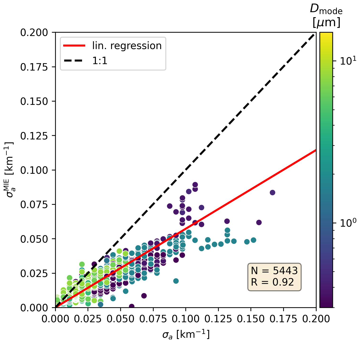
Figure 10 Comparison of ceilometer-derived aerosol extinction coefficients σ_a in 120 m and simulated aerosol extinction coefficients ${\mathit{\sigma }}_{\mathrm{a}}^{\mathrm{Mie}}$ based on in situ aerosol size distributions (1 February–20 June 2023) for an refractive index of 1.5−0i. The inset indicates the number of data points N and the correlation coefficient R. The full red line shows the result of a linear regression. Data points were color-coded according to the diameter D_mode of the size bin with the maximum aerosol mass concentration.

In contrast, the C_m to ${\mathit{\beta }}_{\mathrm{a}}^{\mathrm{Mie}}$ relationships and the $S_{\mathrm{a}}^{\mathrm{Mie}}$ exhibt a much greater dependence on refractive index, compared to the C_m to ${\mathit{\sigma }}_{\mathrm{a}}^{\mathrm{Mie}}$ relationships (Table 3) because of strongly increasing backscattering efficiencies with increasing refractive index. In addition, as already shown by Sundström et al. (2009), for spherical particles in the size range 1–10 µm strong variations and distinct maxima in the phase function in backscattering direction exist, i.e. minima in the lidar ratios. On the other hand, Sundström et al. (2009) demonstrated that these minima do not occur for non-spherical particles which can explain the overall smaller $S_{\mathrm{a}}^{\mathrm{Mie}}$ compared to the AERONET based value of 47 sr used in the retrieval (Sect. 4.2). Note that lidar ratios in a range 40–50 sr are applied in the aforementioned ceilometer networks (Osborne, 2024) in agreement with the value used in this work. However, a column-mean lidar ratio might not be representative of the boundary layer. Nevertheless, the theoretical calculations summarized in Table 3 confirm that the slopes of the empirical linear relationships between C_m and σ_a are robust with regard to variations of refractive indices in the particle phase. This is relevant because a natural aerosol will be composed of particles with different refractive indices and the composition can vary with time. Moreover, the resulting EMC = $\mathrm{1}/r_{\mathrm{3}}$ (Table 3) of (1.3 ± 0.4) m² g⁻¹ are in the range of the literature values.

5.5 Size distributions and potential OPS artefacts

The Mie-theory calculations of the previous section rely on accurately determined size distributions from the OPS measurements. The uncertainties of these measurements are challenging to estimate and are not provided by the manufacturer. But major systematic errors are unlikely relying on careful characterisations by the manufacturer. However, the size range that is covered by the OPS is limited to 0.3–10 µm. The influence of particles greater than 10 µm is uncertain. They are probably correctly discarded because of scattered light signals that are too high. On the other hand, such particles will contribute to the scattered light received by the ceilometer. Similarly, particles smaller than 0.3 µm are not registered because they produce too small signals, but their contribution to the backscatter may still be significant. In addition, particles may be lost in the upstream inlet system before they can enter the OPS. These limitations have in common that they decrease the registered number and mass concentrations of particles that are nonetheless present and potentially relevant for the ceilometer measurements. Without a full characterisation of the size distribution beyond the size range of the OPS, a quantification of the missed aerosol mass concentration and the corresponding simulated aerosol extinction is not meaningful.

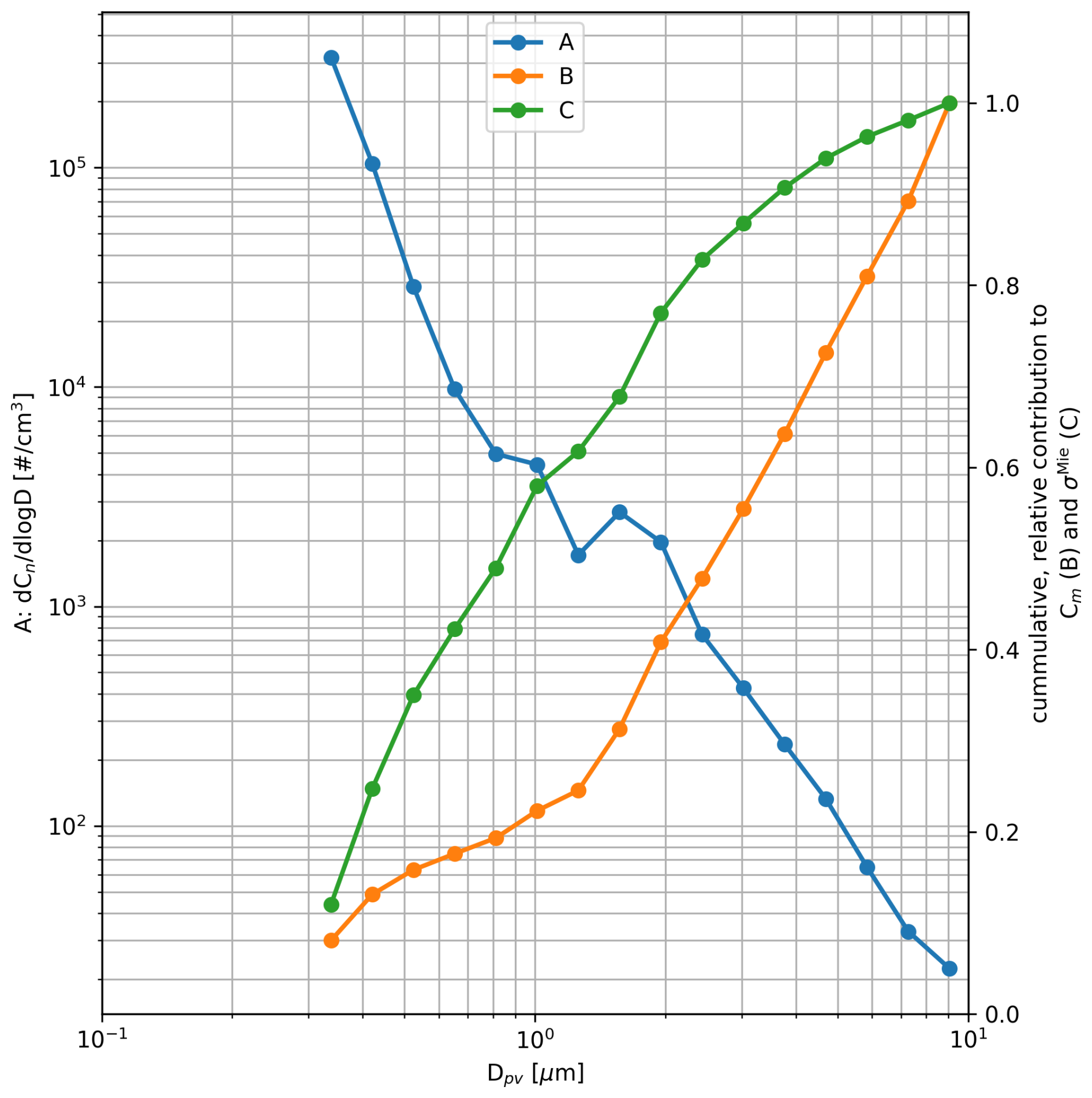
Figure 11 Mean aerosol number size distribution $\mathrm{d}{C}_n/\mathrm{d}\log D$ (A), cumulative, relative contribution to total aerosol mass concentration C_m (B), and cumulative, relative contribution to simulated aerosol extinction coefficients ${\mathit{\sigma }}_{\mathrm{a}}^{\mathrm{Mie}}$ (C) (1 February to 20 June 2023 at the meteorological tower in 120 m).

To illustrate the problem, Fig. 11 depicts the full measurement period's mean aerosol size distribution of this work showing the typical increase of number concentrations towards smaller particle diameters which can be expected to continue to diameters below 0.3 µm and greater than 10 µm. On the right hand axis, the cumulative, relative contributions of the size bins to the measured total aerosol mass concentration C_m and the simulated aerosol extinction coefficient ${\mathit{\sigma }}_{\mathrm{a}}^{\mathrm{Mie}}$ for a refractive index of 1.5 are shown on a linear scale for comparison. The extinction coefficient increase towards the greatest D_pv is already levelling out. The contribution of particles greater than 10 µm is therefore assumed to be limited. On the other hand, the contributions of the size bin with the smallest D_pv are already on the order of 10 % for both aerosol mass concentration and aerosol extinction coefficient. It is therefore plausible that particles with diameters < 0.3 µm have contributed substantially to the ceilometer backscatter and the retrieved extinction coefficients. This could qualitatively explain why the EMC obtained in this work is greater than those in literature and those derived from Mie theory. For the latter the size range limitations seem to be less significant because of compensating effects, i.e. by missing aerosol mass concentration and missing aerosol extinction. Figure 11 also illustrates the apparent D_mode dependence of the σ_a vs. C_m relationships in Figs. 6 and 7. An elevated contribution of particels with D_pv < 1 µm would increase the ${\mathit{\sigma }}_{\mathrm{a}}^{\mathrm{Mie}}$ more strongly than C_m while for particles with D_pv > 2 µm the opposite is the case: the C_m increase would exceed that of ${\mathit{\sigma }}_{\mathrm{a}}^{\mathrm{Mie}}$.

An approach to quantify the contribution of particles < 0.3 µm based on AERONET showed an underestimation of the total volume concentration by this limitation of approximately 20 % as shown in Fig. B2 of the Appendix. However, it should be noted that AERONET refers to column data, whereas the OPS refers to a measurement altitude of 120 m. For this reason, the 20 % are considered as an upper limit, assuming a higher fraction of large particles in the boundary layer.

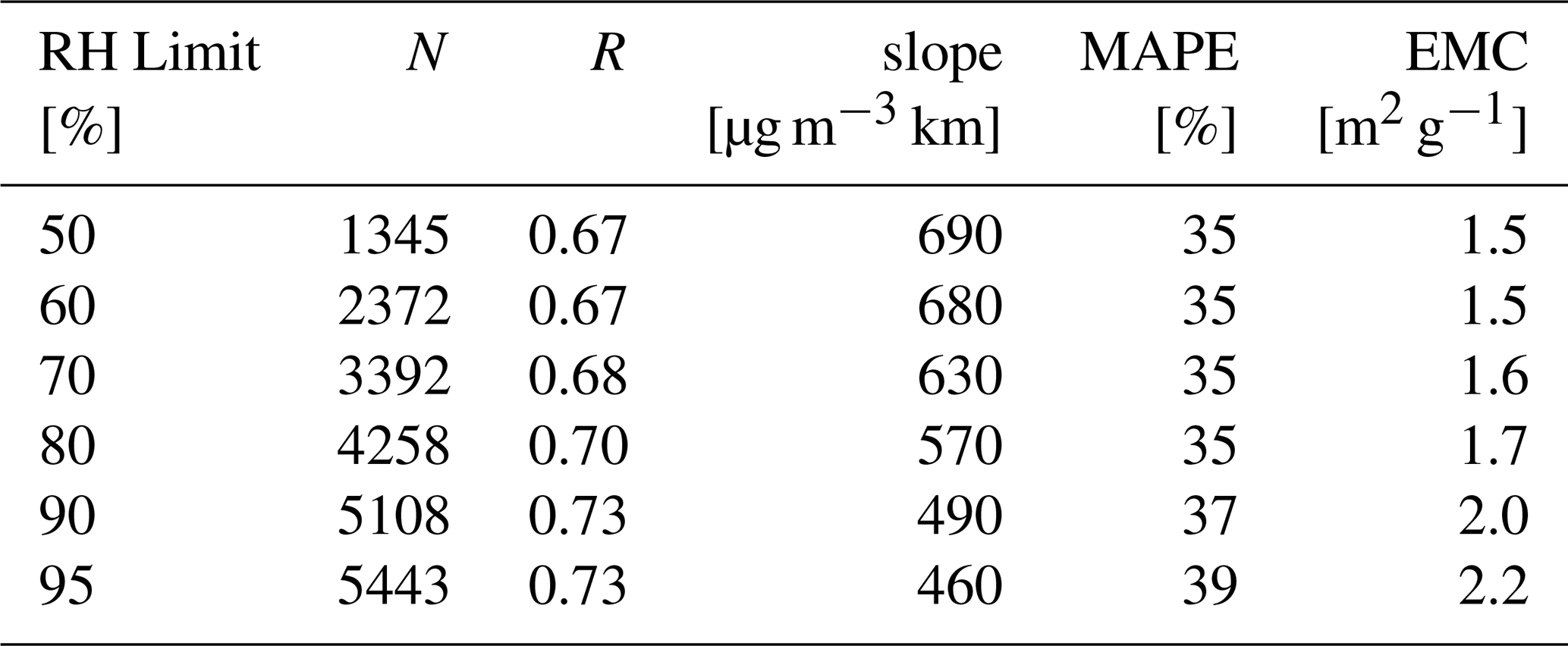
An additional factor is the possibility of unintentional drying of the aerosol in the OPS. The sample stream was not actively dried to preserve the ambient size distribution. Hygroscopic growth within the sampling line is not likely because the temperature inside the box is slightly higher than outside, caused by the waste heat of the instruments. Accordingly, a drop in RH is expected, which could lead to a size-decrease of a fraction of particles prior to detection. It is expected that at higher relative humidities the effect is more pronounced because growth factors typically increase non-linearly with humidity (Titos et al., 2014). To identify a potential bias, the regression analysis for the relation between σ_a and C_m (Eq. 15) was reevaluated as a function of the upper limit in ambient relative humidity. The results are presented in Sect. C in the appendix showing an increase in the slope with decreasing humidity limits. Though within the estimated uncertainties, these data indicate a clear trend consistent with a drying effect by a temperature increase in the OPS. This trend is levelling out towards the lowest limit of 50 % RH. Accordingly, EMC values decrease to values in better agreement with literature.

6 Conclusion

In this study, we assessed different aerosol properties derived from a Vaisala CT25k ceilometer, aiming to evaluate the potential of an existing multi-year ceilometer dataset at the Jülich Observatory for Cloud Evolution (JOYCE) for aerosol remote sensing. The calibration of the ceilometer signal was verified with a liquid cloud calibration (Hopkin et al., 2019). The attenuated backscatter signal was then used to derive aerosol extinction coefficients with a forward inversion method (Li et al., 2021; Mortier, 2022). All tools used in this study are available and can be easily transferred to other ceilometers and ALC networks.

To evaluate the uncertainty of the forward inversion method, an in situ comparison measurement was set up by installing an optical particle sizer (OPS) at 120 m above ground on a meteorological tower in Jülich. This allowed us to measure aerosol size distributions in a range 0.3–10 µm. From the vertical ceilometer profiles, we selected data close to 120 m and compared them to the in situ measurements. A 120 d dataset between 1 February and 20 June 2023 covered by both instruments was analysed. The Cloudnet (Illingworth et al., 2007) target classification was used in combination with a limit in radar reflectivity and relative humidity to exclude the presence of hydrometeors.

In situ aerosol mass concentration C_m was correlated to ceilometer-based attenuated backscatter β_att and aerosol extinction σ_a coefficients with a Pearson correlation coefficient of R = 0.73 for both. Ordinary least square fits resulted in empirical conversion coefficients of 0.18 × 10⁵ µg m⁻³ sr km and 460 µg m⁻³ km for β_att and σ_a respectively. The uncertainties of these conversions were quantified by mean absolute percentage errors of 31 % (β_att) and 39 % (σ_a). However, the σ_a to C_m conversion factor, which corresponds to the inverse of an extinction-to-mass coefficient of (2.2 ± 0.9) m² g⁻¹, is greater by a factor of about 1.8 compared to the literature values (Osborne, 2024). To gain further insight into the role of size distributions and the refractive index on the retrievals, Mie calculations were performed based on in situ measurements. These revealed that σ_a only weakly depends on the refractive index as opposed to the aerosol backscatter coefficients β_a. The ${\mathit{\sigma }}_{\mathrm{a}}^{\mathrm{Mie}}$ to C_m conversion factors based on the Mie calculations were found to be in reasonable agreement with literature values, also indicating a systematic underestimation of the ceilometer-derived conversion factor σ_a to C_m. This disagreement is qualitatively explainable by the limited detection range of the OPS that excludes small particles (< 0.3 µm) that may contribute significantly to the ceilometer signal. Moreover, the OPS mass concentration was found to be underestimated at higher RH, likely caused by a temperature increase inside the instrument.

This study highlights the potential of automatic lidars and ceilometers for aerosol remote sensing. It was confirmed that the retrieval (Mortier, 2022; Li et al., 2021) of σ_a from β_att is viable based on accurate lidar ratios. However, the conversion from σ_a to C_m can introduce significant uncertainties. Additionally, it must be emphasized that the measurement period of 120 d does not resolve possible annual or long-term trends and that the results may be site-specific. Moreover, the instrument used here (Vaisala CT25k) does not represent the performance of modern ceilometers. It is recommended to reevaluate the approach with state-of-the-art instrumentation for future applications. This could be achieved for example by using already existing long-term datasets from other field sites.

Appendix A

Table A1 OPS bin lower limits D_L, upper limits D_U and effective diameters D_pv in µm.

Appendix B: AERONET Comparison

Based on the results of this study, a comparison of ceilometer (CT25k) aerosol optical depth (AOD) with AERONET AOD data was performed. It was found that ceilometer AOD was significantly lower than AERONET AOD (Fig. B1). This can be explained by the reduced signal-to-noise ratio of the CT25k ceilometer at altitudes above about 1.2 km (Markowicz et al., 2008).

The contribution of the different aerosol sizes bins to the total aerosol volume concentration as a comparison between OPS measurements at 120 m and AERONET column data is shown in Fig. B2.

The lower limit of the OPS measurement range at 0.3 µm causes an underestimation of the total volume concentration by approximately 20 %, assuming the same contribution for particles < 0.3 µm for AERONET and the OPS.

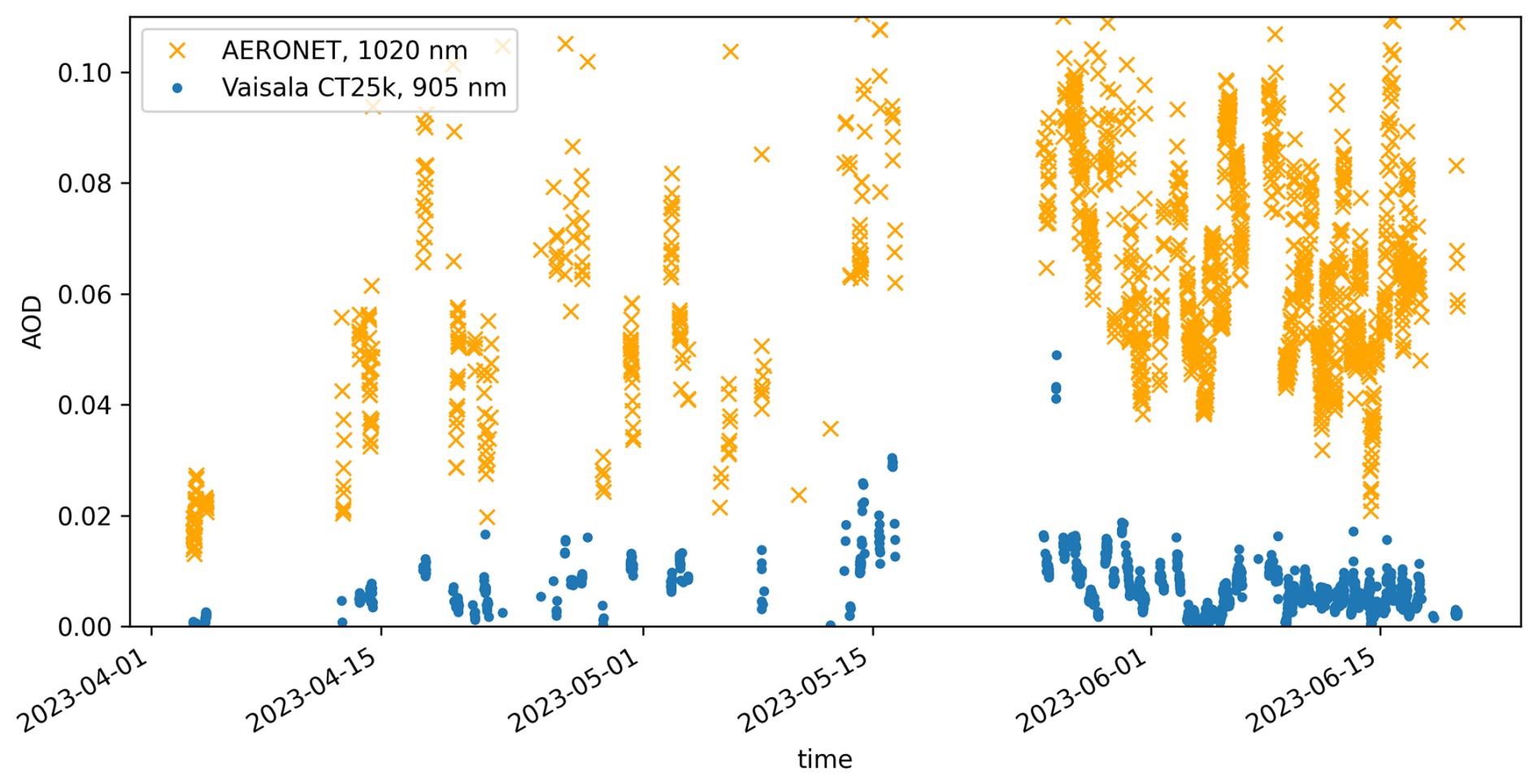
Figure B1 Timeline of aerosol-optical-depth (AOD) from AERONET and vertically integrated σ_a from Vaisala CT25k for the period 1 April to 20 June 2023.

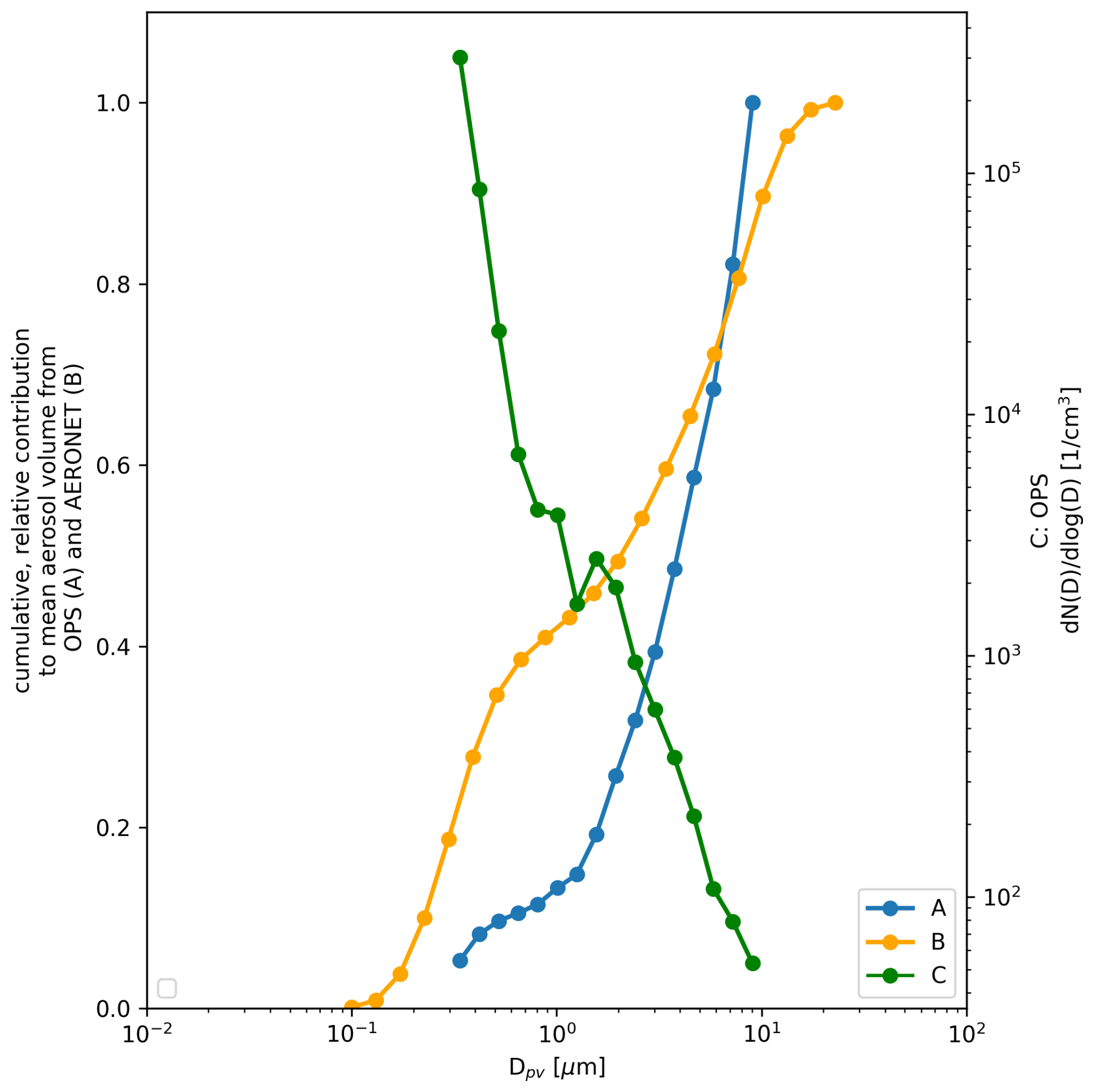
Figure B2 Cumulative, relative contribution to mean aerosol volume from OPS measurements at 120 m (A) and AERONET data (B), C: number size distribution (OPS at 120 m) and column number size distribution (AERONET). All for the period 1 April to 20 June 2023 where AERONET data were available.

Appendix C: Humidity Effects

Table C1 Linear regression analysis of the relation between σ_a and C_m for different upper limits in relative humidity (RH), showing number of data points N, correlation coefficient R, slope of the regression line, uncertainty of the slope and extinction to mass coefficient (EMC).