Evaluating the performance of a cost effective in situ methane sensor for UAS-based systems and its ability to quantify facility-scale emissions

Methane (CH₄) is the second most important greenhouse gas, and accurate quantification of emissions is critical to improve the efficacy of climate mitigation policies. In this study, we thoroughly evaluated the performance of a commercially available in situ CH₄ sensor (LGD-compact A CH₄; Axetris AG, Kaegiswil, Switzerland) for quantifying anthropogenic CH₄ emissions when deployed on an uncrewed aircraft system (UAS). Sensor stability was assessed through laboratory tests under controlled and varying temperature conditions. Under stable conditions, the sensor achieved a precision of 63 ppb at 2 Hz. Furthermore, the tests revealed the necessity of temperature control, and a water vapour correction was derived and applied to ensure accurate measurements. Additionally, the sensor was used to quantify whole-farm CH₄ emissions, by spatially interpolating the measured mole fractions using a Gaussian weighting scheme. This yielded a mean mass emission rate of 4.1 ± 1.6 gCH₄ s⁻¹ averaged over four flights, which was comparable to the value of 4.2 ± 1.1 gCH₄ s⁻¹ obtained from simultaneous flights with the established AirCore technique. Finally, an uncertainty analysis based on the Ornstein-Uhlenbeck method was used to determine the influence of various sources of uncertainty. This analysis revealed that both wind-related uncertainties and background determination can significantly increase the overall uncertainty when not properly constrained. Furthermore, instrumental errors play a dominant role for smaller mass emission rates, while meteorological uncertainties remain significant even with an increased number of flights per day. Nevertheless, careful flight planning, e.g., ensuring extensive sampling outside of the plume and comprehensive wind monitoring, can reduce these uncertainties. Overall, our results demonstrate that a cost-effective sensor integrated onto a UAS can provide reliable CH₄ mass emission rate estimates with uncertainties comparable to those of higher-cost UAS-based systems.

1 Introduction

Methane (CH₄) is the second most important anthropogenic greenhouse gas (GHG) and has received increasing attention due to its relatively short atmospheric lifetime and strong global warming potential (GWP) compared to CO₂. The global average dry air mole fraction of CH₄ reached 1942 ppb ± 2 ppb in 2024 and is expected to increase in the coming years (WMO, 2025). Approximately 60 % of the global CH₄ emissions are linked to human activities, primarily from agriculture, fossil fuel production and use, and waste disposal (Saunois et al., 2025). The observed rise in global CH₄ mole fraction is driven not only by anthropogenic sources but also by changes in natural CH₄ mass emission rates, influenced by ongoing climate change (Ciais et al., 2013). Reducing CH₄ emissions is essential for mitigating climate change and represents a key strategy for limiting global warming to below 2 °C compared to pre-industrial levels (UNEP and CCAC, 2021). To evaluate the effectiveness of mitigation efforts, monitoring CH₄ emissions and identifying their sources are critical.

Despite recent efforts, uncertainties of 20 %–35 % remain in estimates of global annual anthropogenic CH₄ emissions (Saunois et al., 2025). These uncertainties arise from limitations in available data as well as under- and overreporting and misreporting in national inventories. Current CH₄ emission inventories suffer from inconsistencies due to spatial variability in observational data and methodological disparities. Given limitations in existing monitoring systems, approaches focusing on additional measurements and regional studies can help reduce uncertainties in top-down estimates (Saunois et al., 2025; Bousquet et al., 2018; Bruhwiler et al., 2017). Additionally, specific emission sources, such as manure and landfills, exhibit complex emission patterns with substantial diurnal and seasonal variability, making more frequent and reliable measurements necessary (Saunois et al., 2025).

To address these gaps and uncertainties, cost-effective, scalable, and easily maintainable sensor technologies, coupled with robust monitoring methodologies for quantifying anthropogenic CH₄ emissions, are needed. These technologies can be used in more regional studies to evaluate the efficacy of mitigation strategies and monitor emission reductions at finer spatial resolutions (Saunois et al., 2025). International frameworks such as the United Nations Framework Convention on Climate Change (UNFCCC) support the implementation of unified methodologies to improve the accuracy of national inventories. Regular and systematic monitoring is vital for verifying mitigation outcomes and can help detect more fugitive emissions, which are often underrepresented in inventories (Erland et al., 2022).

Uncrewed aircraft systems (UASs) have emerged as valuable tools for addressing data gaps in GHG emission monitoring. Recent advances in sensor technologies have enabled the integration of more lightweight instruments with UAS platforms. These systems offer advantages over alternative approaches (e.g., ground-based or satellite-based observations) by facilitating targeted emission sampling at finer spatial resolutions and bridging the observational gap between ground level and heights up to 120 m (though UASs are capable of flying much higher, regulations typically limit their maximum altitude). Furthermore, UASs are versatile, easy to deploy and maintain, and have a relatively low implementation cost (Villa et al., 2016; Shaw et al., 2021).

Recent UAS-based GHG studies have employed three main sensor deployment strategies: (1) tethered systems connecting an UAS to a ground-based analyser (Shah et al., 2020); (2) semi-continuous sampling equipment (e.g., Active AirCore), mounted directly on UASs for post-flight ground analysis (Andersen et al., 2018; Vinković et al., 2022; Leitner et al., 2023, Han et al., 2024); (3) real-time in situ sensors fully integrated into UAS platforms (Kunz et al., 2018; Allen et al., 2019; Tuzson et al., 2020; Bonne et al., 2024; Scheutz et al., 2025). Although these deployment strategies differ operationally, the mole fractions (observed during flights) require subsequent processing to derive mass emission rate estimates from them, where downwind sampling can be spatially integrated (e.g. following spatial interpolation or grid-square averaging), or modelled using the inverse Gaussian approach (IGA; Nathan et al., 2015; Andersen et al., 2021; Vinković et al., 2022; Bonne et al., 2024; Scheutz et al., 2025; Fosco et al., 2025). This study focuses on the mass balance approach (MBA) because it converts atmospheric mole fractions to mass emission rates following fewer intermediate modelling steps compared to the IGA.

While all mass emission rate quantification techniques introduce inherent uncertainties, wind conditions and spatial distribution of the flight track design consistently emerge as the most influential factors. In general, uncertainties in airborne mass emission rate estimates range from 20 % to 75 % (Vinković et al., 2022; Morales et al., 2022; Scheutz et al., 2025; Liu et al., 2024; Mohammadloo et al., 2025). Still, they can exceed 100 % under challenging conditions such as low wind speeds (<2 m s⁻¹), high wind direction variability (e.g. >30°), or non-uniform sampling (i.e. samples taken at irregular intervals) (Vinković et al., 2022; Morales et al., 2022; Scheutz et al., 2025; Liu et al., 2024; Mohammadloo et al., 2025).

Instrumental or sensor precision is generally considered a minor factor compared to the factors mentioned above, underscoring the importance of investing in accurate wind measurements and thoughtful flight planning rather than prioritising high-precision sensors. Nonetheless, recent research has focused on developing increasingly lightweight and high-precision sensors (Kunz et al., 2018; Tuzson et al., 2020). While these advancements are valuable, their presumed high cost and conceivably high maintenance demands (particularly for open-path optical designs) limit their widespread deployment. In addition, high-precision sensors tend to be heavier, which can reduce flight endurance or require larger and more expensive UASs to accommodate the increase in payload. Evidence suggests that medium-cost, medium-precision sensors (for classification see Appendix A), when combined with accurate wind measurements and optimised flight planning, can achieve mass emission rate estimates with uncertainties comparable to those obtained using high-precision sensors.

In this study, we present and evaluate the performance of a low-cost, medium-precision CH₄ in situ sensor that meets key operational criteria. First, the sensor was characterised in the laboratory to optimise system performance and identify drift. Following extensive testing, the sensor was deployed during a field campaign alongside the Active AirCore to quantify CH₄ emissions from a Dutch dairy farm, a site previously surveyed by Vinković et al. (2022). Using both instruments simultaneously enabled a direct comparison between mass emission rate estimates derived from our medium-precision sensor and those from the established Active AirCore technique, providing new insights into the role of measurement uncertainty in mass emission rate quantification. Finally, a statistical model was used to further investigate the influence of common sources of uncertainty.

2 Laboratory characterisation

Sensor characterisation is essential for improving sensor useability, as laboratory experiments provide insight into its behaviour under varying conditions. In this study, the standard operation of an in situ CH₄ sensor was characterised under stable laboratory conditions. A linearity test was performed to determine the sensor's response over a wide range of concentrations by comparing it to a high-precision reference analyser whose response is known to be linear. An Allan variance analysis provided information on the sensor's precision under baseline conditions (e.g., stable temperature, stable pressure, and no external vibrations), enabling direct comparison across various use cases and setups. The follow-up experiments focused on isolating the effect of different environmental factors on the sensor's output. Water vapour experiments were performed to determine the effect of water vapour on sensor readings and correct the raw observations. Additional Allan variance analyses were performed to compare the sensor's performance under various conditions, e.g., active temperature control, laboratory and in-flight conditions.

2.1 The Axetris in situ methane sensor package

We developed a UAS-mounted sensor package incorporating a commercially available in situ CH₄ sensor (LGD-compact A CH₄; Axetris AG, Kaegiswil, Switzerland), hereafter referred to as the Axetris. The sensor is capable of real-time monitoring at a 2 Hz sampling frequency using a tuneable diode laser spectroscopy (TDLS) technique, which specifically targets the CH₄ absorption wavelength at ∼ 1652 nm.

We integrated the Axetris onto a custom printed circuit board (PCB) designed around an ESP32 microprocessor, enabling logging of data from the Axetris and ancillary sensors. The Axetris reports CH₄ mole fractions, the temperatures of the measurement cell and the interface PCB (which is mounted onto the custom-built PCB). Furthermore, the complete package includes a pressure sensor (AMSYS GmbH model 5915-1200-B) with a precision of ± 0.36 hPa and a measuring range of 800–1200 hPa. A 1200 mAh, 7.4 V Li-ion battery pack powers the whole system. Ambient air was drawn through a filter (Rezist 30/5.0 PTFE-s; Whatman, Freiburg, Germany) into and through the sampling system using a micropump (NMP09; KNF, Freiburg, Germany) at a flow rate of 650 standard cubic centimetre per minute (sccm), ensuring rapid transfer of the sample to and through the measurement cell. With a sampling line volume of ∼ 7 mL and an ambient-pressure cell volume of 19 mL, this configuration yields a time delay of less than 1 s for the sample to reach the measurement cell and a system response time constant of ∼ 1.7 s (∼ 4.2 s t₉₀).

The complete system was housed in a $\mathrm{20}\times \mathrm{20}\times \mathrm{10}$ cm polyethylene (PE) foam enclosure, yielding a relatively lightweight package (1.2 kg). The foam casing acted as a thermal insulator, helping to maintain a stable operating temperature for the analyser. The system had a wireless connection, which provided the ground team with real-time measurements and enabled remote control of critical functions (e.g. set temperature or pump state).

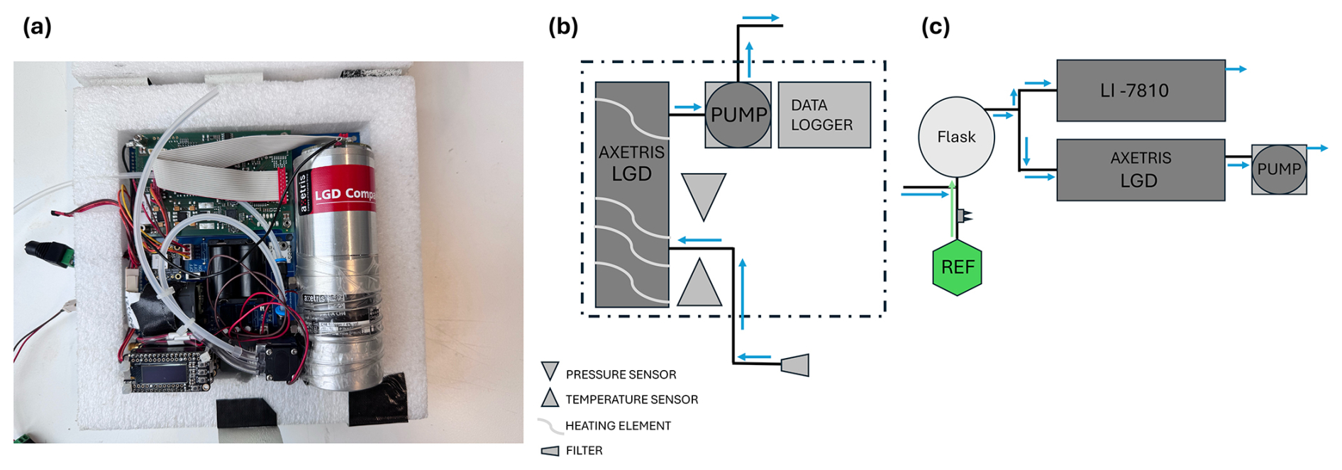
Figure 1 (a) Photograph of the Axetris package. (b) Shematic overview of the Axetris package for UAS applications. The blue arrows show the airflow through the system during measurements. Components in the dotted and dashed lines enclosed area are integrated onto the PCB and enclosed in the PE foam. The datalogger communicates with the Axetris sensor and provides active control of the heating element, including setting and maintaining the desired temperature. (c) Experimental overview for linearity test setup. First, the flask is filled with the reference gas (REF), which has a high CH₄ concentration (indicated by the green arrow). Then, both systems start to sample the air from the flask, while ambient air was drawn in to mix with the high concentration (blue arrows), slowly decreasing the concentration in the flask.

A 1.1 m long low-power heating wire (Nc I 20; ThermoCoax, Suresnes, France) was coiled around the sensor head. This coil was used to maintain the measurement cell's temperature at a predetermined value (typically approximately 10 K above ambient). This adaptation of the sensor improves the systems thermal stability and therewith its measurement performance under ambient temperature fluctuations, as was determined during laboratory characterisation (see Sect. 2.6). A proportional-integral-derivative (PID) controller operated the duty cycle of the heating element, which used the measurement cell temperature (1 mK resolution, 2 Hz) as input. This setup regulated the temperature to within ± 0.005 K from the set-point under lab conditions, and within 0.05 K during flight (Appendix B). Figure 1b presents a schematic of the complete Axetris package.

2.2 LI-7810 trace gas analyser

The LI-7810 trace gas analyser (LI-COR Biosciences, Lincoln, USA) is a high-precision multi-gas analyser that provides continuous measurements of CH₄, CO₂, and H₂O in a durable, portable design. The LI-7810 uses optical feedback cavity enhanced absorption spectroscopy (OF-CEAS). It contains a 6.41 cm³ optical cavity operating at 40 kPa under standard operation (i.e., effective cavity volume of ∼ 2.5 cm³) and 55 °C, and a flow rate of 250 sccm. For this study, the LI-7810 was equipped with a “low flow kit”, which lowered the flow rate to ∼ 70 sccm and changed the system's response time constant to approximately 2.3 s (∼ 5.5 s t₉₀).

The precision, accuracy, and linearity of the LI-7810 analyser under standard operating conditions were evaluated in an extensive report executed by ICOS (ICOS, 2020; we generalise these findings to our specific instrument). From our laboratory tests under controlled conditions and with sufficient warm-up time, we found 1 s precision of 0.1 ppb for CH₄ and 0.2 ppm for CO₂, respectively. The short-term drift over 24 h was <0.7 ppb for CH₄ and <3 ppm for CO₂, respectively_. The 1 s precision of the system operating at reduced flow was the same as under standard operating conditions.

2.3 Linearity of the Axetris

System linearity was verified by connecting both systems to a flask filled with a high CH₄ concentration (∼ 81 ppm). The concentration inside the flask was then gradually reduced by allowing ambient air to enter, while the Axetris and the LI-7810 sampled it (see Fig. 1c for experimental setup). The LI-7810 system linearity was confirmed by extensive laboratory tests (using a different instrument of the same type; ICOS, 2020). These tests enabled direct comparison of the systems' response across a wide range of concentrations (2 to 20 ppm). Figure 1c shows an overview of the experimental setup.

The linearity test revealed strong agreement between the Axetris and LI-7810, with a correlation coefficient of 0.996 (Fig. C1) and a residual plot showing the linearity of the system over the concentration range considered (Fig. C2). The linear equation between the two systems is as follows:

$${\mathrm{CH}}_{{\mathrm{4}}_{\mathrm{Ax}}}=\mathrm{1.00}{\mathrm{CH}}_{{\mathrm{4}}_{\mathrm{LIC}}}+\mathrm{120}$$

where CH${}_{{\mathrm{4}}_{\mathrm{Ax}}}$ refers to the raw Axetris observations and CH${}_{{\mathrm{4}}_{\mathrm{LIC}}}$ the LI-7810 CH₄ observations. The slope confirms linearity between the two systems, while the intercept indicates the bias between them. This bias (120 ppb) can be easily dealt with through calibration. The results confirm the reliability of the Axetris under controlled conditions and its ability to measure high CH₄ concentrations with strong linearity to the LI-7810 (Appendix C; Fig. C1).

2.4 Water vapour corrections

Water vapour can affect gas sensor readings in two ways: (1) by dilution of trace gas concentrations and (2) through more complex spectroscopic effects. The influence varies depending on the sensor type and the correction algorithms implemented by the sensor manufacturer (Butenhoff and Khalil, 2002). To characterise the effect of water vapour on the Axetris response and derive an empirical correction, we conducted a controlled water-droplet test.

While performing the water droplet test, the Axetris and the LI-7810 sampled air from a gas cylinder containing a high concentration of CH₄ (∼ 81 ppm). A Swagelok compartment containing a wet paper towel was placed between the sampling lines to introduce water vapour into the otherwise dry gas stream (Appendix D; Fig. D1 for experimental set-up). The compartment was gradually heated using a hairdryer to increase humidity levels, measured with the LI-7810. Water vapour concentrations ranged from 0.06 % to 1.4 %.

The dry value of the reference gas was determined by sampling the cylinder air without the Swagelok compartment. The LI-7810 reported a water vapour concentration of 0.004 % and a CH₄ concentration of 81.7 ppm. We quantified the influence of water vapour on CH₄ measurements by determining the linear relationship between: (1) the ratio of wet-air CH₄ concentration (Axetris) to dry-air CH₄ concentrations (LI-7810) and (2) water vapour concentration, as follows:

$${\displaystyle \frac{{\mathrm{CH}}_{\mathrm{4}\mathrm{wet}}}{{\mathrm{CH}}_{\mathrm{4}\mathrm{dry}}}}=\mathrm{1}+a{\mathrm{H}}_{\mathrm{2}}\mathrm{O}$$

with $a=-\mathrm{0.013}\pm \mathrm{0.00008}{\mathit{\%}}^{-\mathrm{1}}$. Figure D2 in the Appendix depicts the linear regression.

As mentioned, water vapour affects the measurements in two different ways (Chen et al., 2010; Rella et al., 2013). At 81.7 ppm CH₄, this relationship corrects mainly for the water vapour dilution effect, although other effects, including spectral interference and H₂O calibration, account for ∼ 30 % of the dilution effect. For field applications, we correct ambient air sample measurements using the derived correction function to convert the measurements in humid air to dry air mole fractions. In practice, water vapour concentrations were either measured directly in the field (using the LI-7810) but could also be taken from nearby meteorological stations. With this, we assume that the non-dilution part of the water vapour correction remains the same at ambient levels as at high concentrations. Although this approach may not capture the full variability of water vapour, it is expected to adequately account for the most significant sources of water vapour related variability in the measurements. Any residual error introduced by this simplification is considered negligible, especially when compared to larger sources of uncertainty, such as wind variability.

2.5 System precision

The system's precision can be determined by operating it under stable conditions while sampling a dry reference gas with a known concentration over a longer period. The obtained time series was further analysed using the Allan variance method. The method is a commonly used statistical tool for assessing frequency stability and identifying noise characteristics in measurement systems (Allan, 1966). It provides insight into the noise, stability, and drift of the Axetris, helping distinguish between random noise and systematic drift and informing the user about the optimal calibration frequency. In addition to the stable laboratory test, the sensor was deployed underneath an UAS while it sampled a reference gas from a calibration bag. These tests gave insight into the sensor's precision when experiencing flight induced vibrations and aerodynamic disturbances. The calibration bag used is a ∼ 1 L multilayer gas sampling bag (Supelco Inc.) that was tested and used by Hooghiem et al. (2018) for high-precision stratospheric measurements of CO₂, CH₄, and CO.

The laboratory test lasted for 16 h, with a temperature of 25 ± 0.1 °C and a pressure of 1.02 ± 0.001 bar (as recorded by the sensors on the PCB), while pushing gas through the Axetris at a flow rate of 70 sccm. The sensors precision during UAS deployment was determined for each of three consecutive flights, each lasting 20 min and varying flight patterns. Results were processed in MATLAB using the allanvar function (version R2019a), which yielded the Allan variance (σ(τ)²) and the corresponding averaging time (τ). To aid with the interpretability of the resulting figures, we converted the Allan variance to the Allan deviation (in ppb; √σ(τ)²).

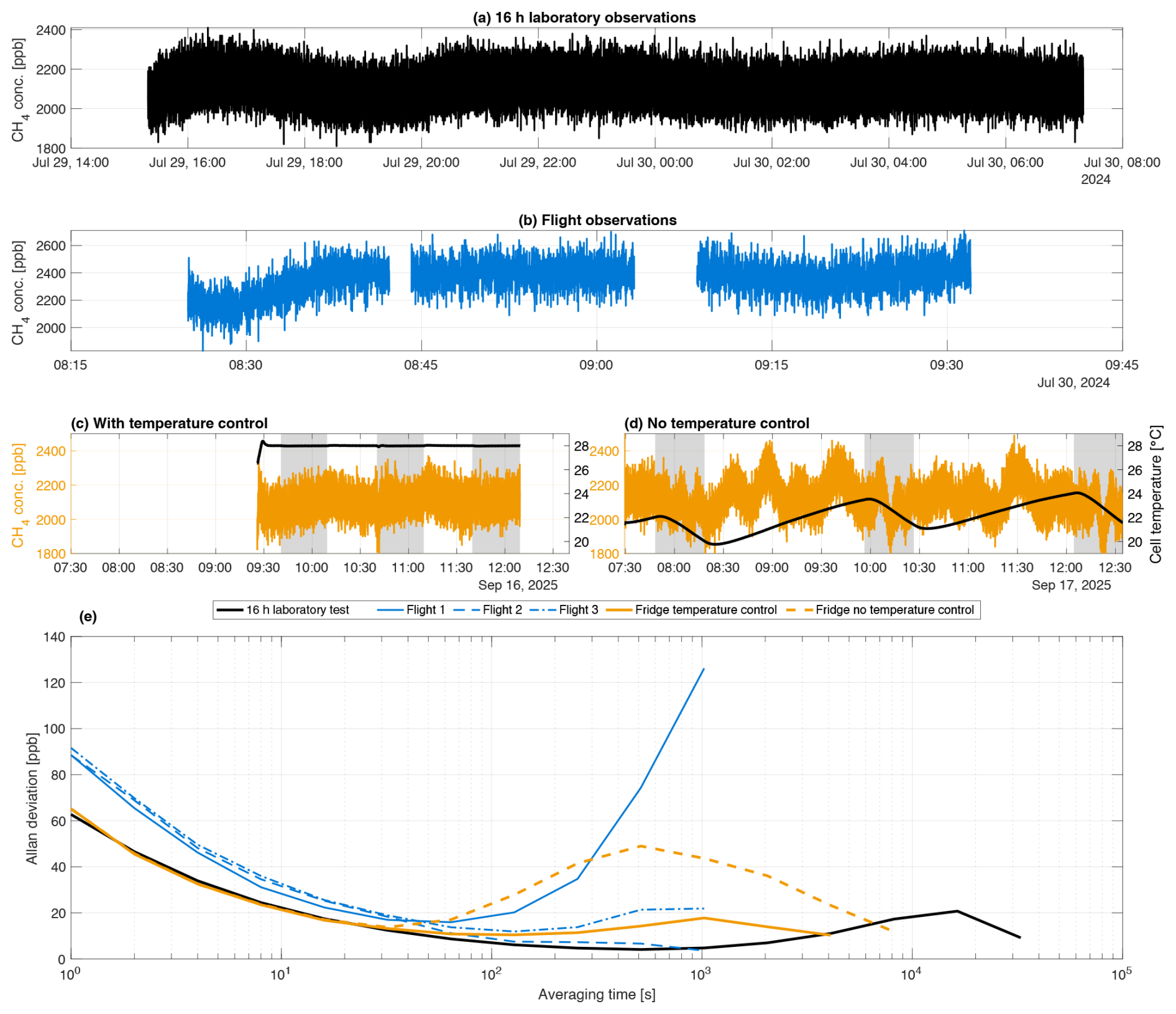
Figure 2 Overview of sensor observations and Allan deviation results. (a) Axetris measurements over sixteen hours during stable laboratory conditions, without active temperature control. (b) Axetris measurements (blue) during the in-flight stability tests (without active temperature control). (c) Axetris measurements (orange) with active temperature control and corresponding cell temperature (black). (d) Axetris measurements (orange) without active temperature control and corresponding cell temperature (black). Grey-shaded areas indicate 30 min periods inside the fridge (7.5 °C). (e) Allan deviation plots of the stable laboratory measurements (black), during flight conditions (blue; without temperature control), and the fridge experiments with (orange) and without (dashed orange) temperature control.

Figure 2 shows the Allan deviation results obtained under stable laboratory conditions (16 h dataset) and during in-flight operation. Figure 2a shows the recorded CH₄ measurements during the 16 h test and depicts a slow drift in the initial hours of the observations. After being turned on, the system stabilises its cell temperature during the warm-up period. However, the observed drift cannot be linked to this phase, as the system had been on for several hours before the experiment.

Figure 2e shows a precision of 63 ppb at 1 s averaging, improving to 4 ppb at 512 s averaging under stable laboratory conditions. Beyond this duration, the sensor's precision becomes drift-dominated. To maintain measurement precision below 10 ppb, calibration every hour is required (Appendix E). However, when operating the sensor during UAS deployment, its precision decreases. Its performance under flight conditions may differ due to additional pressure and temperature variations (1.01 ± 0.004 bar; 28.4 ± 0.7 °C), as well as vibrations of the UAS. In comparison, the Allan deviation analysis of in-flight data (sampled from a calibration bag) shows the sensor's precision of 91 ppb at a 1 s interval, reaching a minimum of 11 ppb after 128 s. These results demonstrate the sensor's performance without additional temperature control and show that flight induced disturbances may reduce its precision (Fig. 2e).

2.6 Temperature dependency

Temperature variability is readily observed to affect sensor performance significantly. During routine use, this may lead to biases whenever ambient conditions change, for instance, when moving the sensor from a car to an UAS. To demonstrate this effect and the efficacy of a temperature control system, we conducted controlled experiments. Here, the Axetris was exposed to sudden temperature changes while continuously sampling a reference gas. The conditions encountered during UAS deployment were simulated by transferring the sensor from a room-temperature environment to a fridge (7.5 °C). Airflow around the sensor package (i.e., all components inside a foam casing) was mimicked by placing a small fan inside the fridge. In the experiment, we compared (1) actively heating of the sensor to 28 °C using the heating wire to (2) no heating and only relying on the dampening effect of the foam casing to provide temperature stability. The Axetris' output was continuously monitored, and the sensor was only transferred after readings had stabilised for a period of ∼ 10 min. Each configuration was tested in three independent runs, with the sensor exposed to the cooler environment for 30 min per run.

Figure 2c and d show the time series of the temperature-dependence experiment, illustrating the necessity of active cell temperature control for stable Axetris measurements under varying ambient conditions. During the experiment, the fridge temperature was 7.6 ± 0.5 °C and the laboratory temperature was 21.4 ± 0.5 °C. Figure 2c depicts the Axetris observations with the cell temperature actively controlled at 28 °C. In contrast, Fig. 2d presents the measurements without active temperature control, where irregular and non-linear behaviour is observed. In both panels, the shaded areas indicate the 30 min periods during which the sensor was placed inside the fridge.

Figure 2e shows the Allan deviation plots for the periods when the Axetris was inside the fridge. As expected, the three tests with active temperature control (orange solid line) exhibit decreasing Allan deviations, reaching a minimum of 6 ppb at τ=256 s, and stays below ± 18 ppb for the duration of the experiment. This is similar to the behaviour observed during the laboratory condition test (black solid line). Without temperature control (orange dashed lines), the Allan deviation initially follows the same downward trend. However, it reaches its minimum of 13 ppb at τ=64 s. Longer averaging times causes the drift to rise sharply, rising to approximately ± 50 ppb.

Active temperature control improves sensor stability and extends the averaging time over which the lowest precision is achieved. In addition, the heating element effectively suppresses the random oscillations observed without temperature control. The random oscillations are detrimental to the system's performance and are too complex to correct. Therefore, observations made when the sensor behaves in this way cannot be used for accurate mass emission rate estimation. Finally, in the absence of temperature control, the sensor's stabilisation period after exposure to the colder environment is substantially longer (Fig. 2d), whereas with active temperature control, the sensor is immediately ready for deployment, improving its practicality.

3 Field validation of the Axetris sensor

The laboratory characterisation and addition of the active temperature control improved the sensor's observation quality and optimised its performance for in-field deployment. These improvements were then tested during a field validation of the Axetris sensor, comparing its performance with that of the proven Active AirCore technique (Andersen et al., 2018; Morales et al., 2022; Vinković et al., 2022). Both instruments were deployed simultaneously underneath a UAS during flights at a dairy farm in the north of the Netherlands. These tests allowed for a direct comparison of the two systems for quantifying CH₄ emissions from the whole farm.

3.1 Field site

The dairy cow farm investigated during this study is located in the village of Grijpskerk, approximately 20 km north-west of the city of Groningen. Planar pastures and cropland surround the farm, with clear upwind areas, making it an ideal location for UAS-based quantification. Emissions from the farm were previously quantified by Vinković et al. (2022), allowing us to identify similarities and differences in the emission pattern of the farm. During this study, three main CH₄ sources were identified: a barn with all dairy cows (225 cows), a barn with other cattle (25 dry cows and 132 heifers), and three manure cellars. These sources were also of interest to Vinković et al. (2022).

3.2 UAS system

The sensor package was mounted underneath a DJI Matrice 600 hexacopter UAS using two straps while the sampling inlet was connected to a sampling tube pulled through a 1 m long carbon fibre rod. The inlet is located 50 cm upwind of the propeller downwash column. The UAS has a maximum payload capacity of 6 kg, well above the Axetris package's weight, and a wind speed resistance of 8 m s⁻¹. The typical flight duration decreased from 35 min (unloaded) to 20–25 min when carrying the Axetris package and further decreased when the active AirCore was flown simultaneously. An anemometer (LI-550 TriSonica, LI-COR Biosciences, Lincoln, USA) was mounted on a 1 m tall carbon fibre rod extending from the UAS to obtain in-flight wind speed and wind direction measurements.

3.3 Meteorological measurements

The measurement hours (on 29 July 2025) had moderate, constant wind (∼ 4 m s⁻¹), mild temperature (∼ 16 °C), and were mostly dry, and possibly mildly convective. Meteorological data were obtained from both ground-based and UAS-mounted sensors, including: (1) a 3D sonic anemometer (WindMaster Pro; Gill Instruments, Hampshire, UK) placed near the farm, which recorded continuous wind speed and direction at 10 Hz at a height above ground level of 3 m, and (2) the UAS's onboard wind sensor, i.e. the TriSonica, which provided complementary in-flight measurements. The WindMaster Pro observations were used to anchor a logarithmic wind profile based on the theoretical formulation of Stull (1988).

$$\begin{array}{}\text{(1)}& u\left(z_i\right)=u_{\mathrm{ref}}{\displaystyle \frac{\ln \left(\frac{z_i}{z_{\mathrm{0}}}\right)}{\ln \left(\frac{z_{\mathrm{ref}}}{z_{\mathrm{0}}}\right)}}\end{array}$$

Equation (1) assumes neutral atmospheric stability and a homogenous surface. A surface roughness length z₀=0.15 m was used, which is representative of conditions between low and tall agricultural crops (Wieringa, 1992). The reference wind speed u_ref was derived as the average of the WindMaster Pro observations for the duration of each of the flights (Table 1), and z_ref denotes the height above ground level of these reference observations (z_ref=3 m), and z_i includes the considered heights. This logarithmic wind profile is used for calculation of mass emission rates.

To visually assess the appropriateness of the logarithmic profile, we plot it together with the TriSonica measurements and observations from the two nearby Royal Netherlands Meteorological Institute (KNMI) stations (Appendix F). Raw TriSonica measurements were converted to true wind speed and direction by accounting for the UAS's motion and orientation. Overall, the TriSonica observations show a clear increase in wind speed with altitude, resembling the cardinal feature of the logarithmic profile. The uncertainty bounds of the TriSonica data overlap with the profile, indicating that our assumptions about the logarithmic profile are reasonable under the flight conditions. In addition, observations (reported as u₁₀) from the KNMI stations at Eelde (∼ 30 km SE from the farm) and Leeuwarden (∼ 25 km W) were included in Appendix F. The TriSonica observations corroborate the existence of a logarithmic profile, warranting its use over that of a single wind speed value over the full altitude range.

3.4 Active AirCore

The active AirCore system provides semi-continuous sampling and analysis of various trace gases. In this study, we measured CH₄ mole fractions along flight trajectories using an upgraded version of the system described by Andersen et al. (2018). The AirCore consists of a 95 m stainless steel coil (635 mL volume) that samples ambient air at a controlled flow rate of ∼ 23 sccm, allowing approximately 27 min of flight time. However, due to the UASs battery and the total payload, the maximum flight duration was only 15 min. After landing, the AirCore was connected to the LI-7810 to measure the CH₄ mole fractions from the collected air samples. The samples were pulled through the AirCore and into the analyser and followed by one of the two available gas mixtures from cylinders. Alternating, per flight, between the two gas tanks enabled easy identification of the start and end points of the analysis. In this manner, two flights per hour can be achieved.

A primary challenge of the active AirCore technique is assigning the CH₄ concentration readings from the gas analyser (LI-7180) to the flight trajectory. In principle, simultaneous flights with the Axetris and the AirCore allow for improved alignment, as in situ observations permit direct temporal and geospatial projection of AirCore measurements. This method was indeed implemented here but did not appreciably improve the results of the nominal mapping, shifting the assigned timestamps of the project AirCore data by less than 2 s (i.e., ∼ 5 m horizontal). Information about the AirCore pump status helped to correctly link the AirCore observations to the UAS's geospatial position. Incorrectly selecting the LI-7810 timestamps corresponding to the ambient sample introduced a larger uncertainty.

3.5 Flight strategy

The UAS equipped with both sensor packages was flown downwind of the dairy farm at a constant speed of 3 ± 0.5 m s⁻¹ while maintaining stable orientation and with the sampling inlet pointed into the wind. The UAS flight track was oriented approximately perpendicular to the wind direction to achieve optimal cross-sectional sampling. A wireless connection enabled the ground team to monitor CH₄ concentrations in real time and ensure sufficient sampling outside the plume, which is essential for obtaining sufficient background data and properly constraining the extent of the plume. Continuous sampling was conducted along transects at multiple altitudes, typically at 5 m vertical intervals. The flights were conducted under light to moderate wind conditions (3.7 ± 1.4 m s⁻¹, NW to WNW; Appendix F) and consisted of 12 transects between 4 and 60 m above ground level at approximately 120 m downwind of the farm (Appendix I).

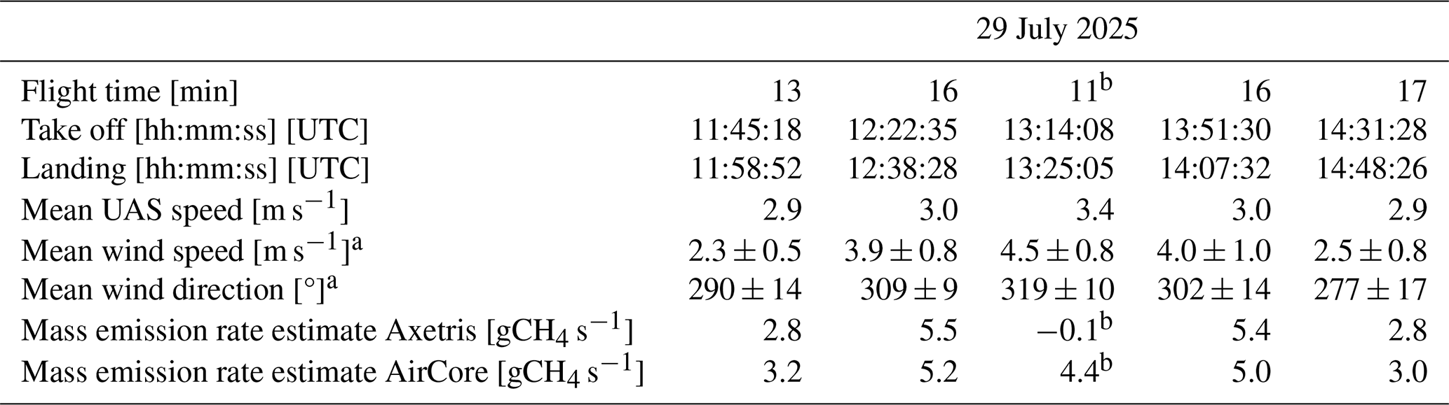
A total of five UAS flights were performed on the 29 July 2025, with flight duration ranging from 11 to 17 min, depending on battery capacity, meteorological conditions, and payload mass. Weather conditions were cloudy, with occasional rain and temperatures ranging from 18 to 21 °C. Typical wind speed was 4 m s⁻¹ (maximum 8.5 m s⁻¹) at 3 m above ground level (Appendix F). Table 1 provides an overview of the flight characteristics.

Table 1 Summary of the five downwind flights conducted on 29 July 2025.

^a The wind direction and speed are obtained from the 3D sonic anemometer and observed at a height of 3 m. ^b Temperature control failed during flight 3, this flight will be excluded from further analysis.

3.6 Spatial interpolation

Spatial interpolation is crucial for estimating CH₄ mole fractions at unsampled locations, which are subsequently used to calculate the total mass emission rate. After applying the corrections as stated in Sect. 2 (i.e. compensation for water vapour dilution and thermal stability), we interpolated the observed CH₄ enhancements onto a grid using a Gaussian weighting scheme with finite spatial influence. This approach produces smoother concentration fields than alternative techniques such as inverse distance weighting (Di Piazza et al., 2011), because the Gaussian kernel gradually reduces the influence of distant measurement points rather than abruptly discarding their contributions. The weight assigned to each observation is computed as:

$$\begin{array}{}\text{(2)}& {\mathit{\omega }}_j=\exp \left(-\left[{\left({\displaystyle \frac{x_i-x_j}{r_{\inf }^x}}\right)}^{\mathrm{2}}+{\left({\displaystyle \frac{y_i-y_j}{r_{\inf }^y}}\right)}^{\mathrm{2}}\right]\right)\end{array}$$

where (x_jy_j) are the coordinates of the observations, (x_iy_i) are the location of the grid cell, and $r_{\inf }^x$, $r_{\inf }^y$ are the influence radii in the vertical and horizontal direction, respectively. Furthermore, observations outside a predefined cutoff radius are excluded from the interpolation, effectively spatially limiting the influence of each observation. This limit is required because the Gaussian kernel gradually reduces in strength but never reaches zero.

The estimated CH₄ mole fraction, c_i, at each grid location is then computed as a weighted average using:

$$\begin{array}{}\text{(3)}& c_i={\displaystyle \frac{{\sum }_{j=\mathrm{1}}^{N_i}{\mathit{\omega }}_j{z}_j}{{\sum }_{j=\mathrm{1}}^{N_i}{\mathit{\omega }}_j}}\end{array}$$

where z_j is the observed value and N_i is the set of observations that fall within the cutoff radius of grid points i. Grid cells with no contributing observations (i.e., beyond the cutoff radius of the nearest measurement) are assigned missing values (NaN) and excluded from subsequent analysis.

3.7 Mass balance

The spatially interpolated CH₄ concentrations were used to estimate the farm's total CH₄ emission rate by implementing the results in the mass balance approach (MBA) similar to Nathan et al. (2015) and Vinković et al. (2022). The following equation gives the MBA:

$$\begin{array}{}\text{(4)}& \begin{array}{rl}{Q}_{{\mathrm{CH}}_{\mathrm{4}}}& =\cos \left(\mathit{\theta }\right){\displaystyle \frac{M_{{\mathrm{CH}}_{\mathrm{4}}}}{M_{\mathrm{vol}}}}{F}_{\mathrm{ppb}}{\sum }_{i=\mathrm{1}}^{N_y}{\sum }_{j=\mathrm{1}}^{N_x}\\ & \mathrm{\Delta }x\mathrm{\Delta }y\mathrm{\Delta }{c}_{i,j}{u}_{\mathrm{prof}}\left(y_i\right)\end{array}\end{array}$$

where u_prof is the logarithmic wind profile (in m s⁻¹, as described in Eq. 1), θ the angle between the mean wind direction and the direction perpendicular to the flight track, Δx and Δz represent the horizontal and vertical grid size of the integration plane (2 by 2 m in this study), the molar mass of methane is given by $M_{{\mathrm{CH}}_{\mathrm{4}}}$, Δc gives the dry CH₄ mole fraction enhancement above the background in ppb, F_ppb is the unitless conversion factor from ppb to mole fraction and M_vol gives the molar volume and is defined as:

$$\begin{array}{}\text{(5)}& M_{\mathrm{vol}}={\displaystyle \frac{RT}{P(\mathrm{1}-{\mathrm{H}}_{\mathrm{2}}\mathrm{O})}}\end{array}$$

where R is the universal gas constant, T is the ambient temperature in Kelvin, P is the ambient pressure in Pascal, and H₂O is the mole fraction of water vapour in the air. In this work, a constant wind direction was assumed during flight, allowing the corresponding term to be placed outside of the summation. Additionally, the ambient H₂O mole fractions used to determine the dry-air correction of Δc mole fraction and the calculation of M_vol were obtained using the LI-7810 analyser. If in-field observations of [H₂O] are not possible, a mean value may be approximated from RH % observations from nearby meteorological stations. All other meteorological parameters were recorded during flight and used to calculate the CH₄ mass emission rate $Q_{{\mathrm{CH}}_{\mathrm{4}}}$ through the integrated plane. The obtained mass emission rate is interpreted to equal the emission at the farm and are reported in grams per second (g s⁻¹).

As stated, Δc represents the dry CH₄ mole fraction enhancement above background. For the AirCore, the background concentration was determined as the 10th percentile of the observations, under the assumption that the UAS sampled beyond the plume boundaries. The 10th percentile method is not suitable for the Axetris due to its higher noise level. Applying this method to the Axetris observations would result in an overestimated mass emission rate, as the method selects the observations that lie at the lower bound of the sensors noise.

Rather for the Axetris, the background was defined as the mean CH₄ mole fraction from the measurements obtained outside the plume boundaries. To identify these regions, CH₄ concentrations were plotted against the horizontal distance travelled, and the area with the lowest values was selected based on visual inspection and all observations in the area were averaged (Appendix G). Under ideal conditions, this plot reveals a distinct separation between elevated CH₄ values (associated with plume observations) and lower, stable values representing the background. By assuming that the lower CH₄ observations correspond to the background and including a large number of data points, the estimated background value is expected to closely approximate the true atmospheric background and to have a low uncertainty.

The averaging background method is not ideal for the Active AirCore due to its intrinsic signal smoothing (Morales et al., 2022). To use the same method, longer sampling outside of the plume should be part of the flight strategy (Appendix G), limiting the collection of plume samples. The AirCore and Axetris methods report different backgrounds, since both instruments were only approximately calibrated during the field campaign. Mass emission rate quantifications for each sensor are conducted with its respective technique and background concentration.

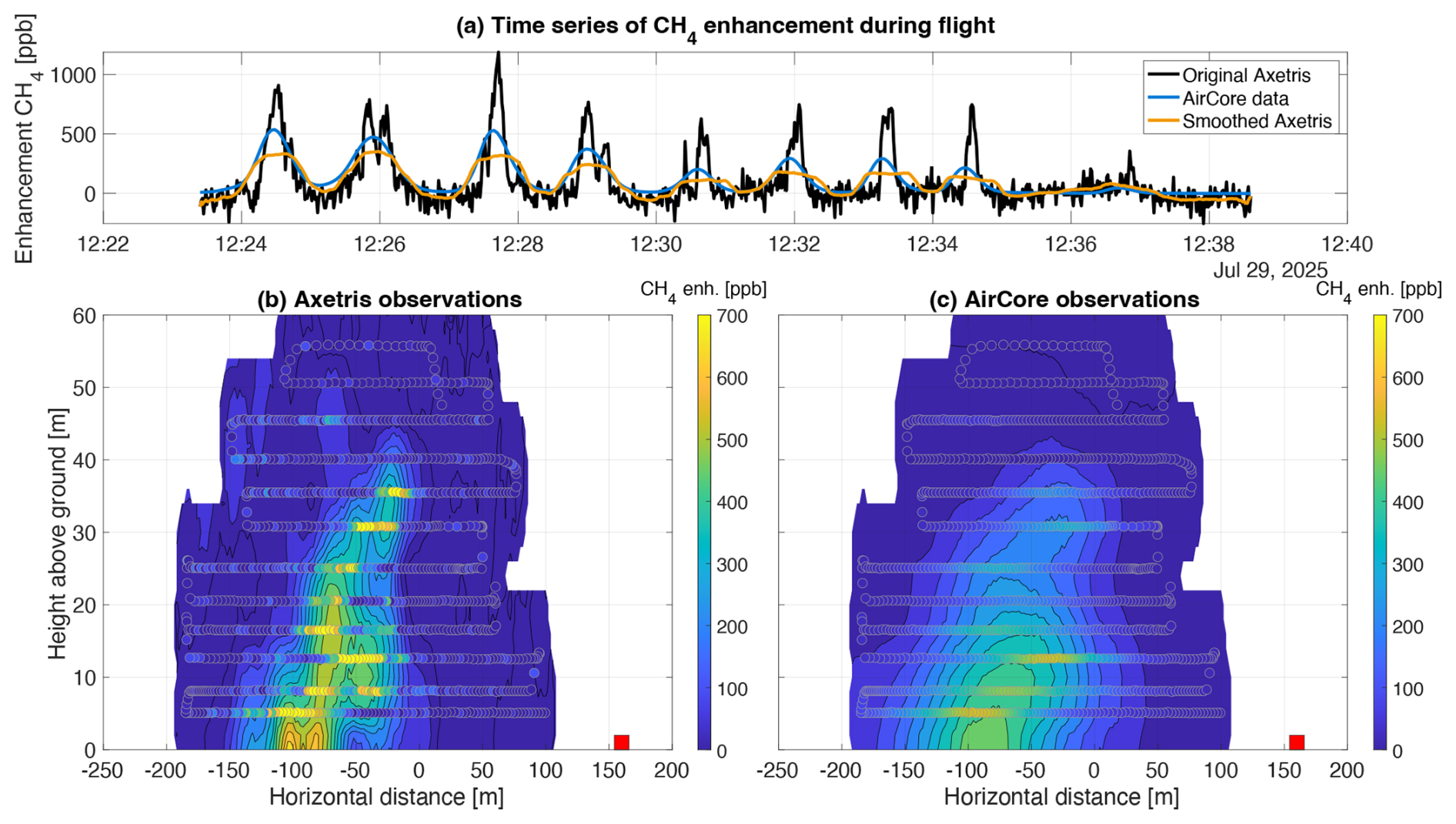
Figure 3 Observations and the spatially interpolated data from the second flight conducted on 29 July 2025. The horizontal distance is referenced to the projected location of the barn centre (defined as 0 m). The sampled plane is located 120 m downwind of the farm. The red square shows the take-off location relative to the projected location of the barn centre. (not in-plane). (a) shows the measurement series of CH₄ enhancements of the AirCore (blue; projected onto the Axetris flight times), the dry Axetris data (black), and smoothed Axetris data (orange). (b) Spatial interpolation of the dry Axetris data, with discrete measurement points overlaid to visualise the flight track. (c) Spatial interpolation of the AirCore data, with discrete measurement points overlaid to visualise the flight track.

3.8 Comparison of results of Axetris and AirCore

An illustrative overview of the second of the five UAS flights is shown in Fig. 3. The top panel (Fig. 3a) shows the AirCore observations (blue), dry Axetris observations (black) and the smoothed Axetris (orange). The latter series is plotted merely for illustrating the likeliness between it and the AirCore observations. Both the AirCore and the Axetris measurement series clearly show repeated detection of the CH₄ plume.

The smoothed Axetris series was obtained using locally weighted scatterplot smoothing (LOWESS) of the raw signal. The AirCore measurements covary closely with the smoothed in situ sensor data, illustrating the accuracy of the temporal projection methodology. A smoothing window size of 50 samples was found to yield an optimal likeliness of the Axetris to the AirCore data (Appendix H), with a correlation coefficient of 0.94, and RMSE of 36.6 ppb over all flights. When solely looking at the difference in the enhancement, the mean difference reduces from 89 ± 39 ppb (1σ; over all flights) to 26 ± 44 ppb (1σ; over all flights). The higher mean difference in the dry concentration data may be attributed to the lack of calibration of the sensors. The large standard deviation may be attributed to (1) the differences in response time, as the LOWESS for the Axetris only approximates the Taylor and molecular dispersion that appears in the AirCore and the additional smearing effect inside the measurement cell of the LI-7810 (Andersen et al., 2018) and (2) a slight temporal shift between the two signals that cannot be completely eliminated also contributes to the difference. We use only the dry signal in subsequent analyses.

Figure 3b and c show the spatially interpolated Axetris and Active AirCore data, respectively. The AirCore method produces a wide and smooth plume compared to the narrow and more sharply enhanced plume derived from the Axetris data (Fig. 3b). The results of these interpolations were used with the MB equation (Eq. 4) and the logarithmic wind profile (inferred from the WindMaster Pro data) to calculate the full farm mass emission rate, reported in Table 1. The emissions estimates derived by the two methods (AirCore, Axetris) differed by less than 10 %, both for individual flights as for the mean of flights.

This variability in wind speed and direction can influence the mass emission rate estimate, leading to an over- or underestimation of the emission (Mohammadloo et al., 2025). A change in wind direction can cause the plume centre to shift, increasing the probability of sampling the full plume multiple times during flight or missing it altogether. Performing multiple passes across different altitudes, these plume-displacements can be captured and accounted for in the final mass emission rate estimate (Scheutz et al., 2025). Variability in the wind speed alters both the plume advection and dispersion. Higher wind speeds tend to elongate the plume and dilute observed concentrations, whereas lower wind speeds have the opposite effect (Stull, 1988).

The emission rates of the farm estimated from individual flights ranged from 3.5 to 5.2 gCH₄ s⁻¹ for the AirCore method and from 2.8 to 5.5 gCH₄ s⁻¹ for the Axetris method (Appendix J). Flight 3 was excluded from the analysis due to a failure in the active temperature control, causing the Axetris sensor to drift and rendering the observations invalid. The subsequent analysis is based on four of the five flights. The average emission rate across all quantifications using the active AirCore is 4.2±1.1 gCH₄ s⁻¹ (1σ; n=4). The Axetris yielded a similar value of 4.1 ± 1.6 gCH₄ s⁻¹ (1σ; n=4), when using their respective background concentrations. When averaging all four flights, the mass emission rate estimates and the standard deviation between them are similar, indicating that the Axetris can determine mass emission rates comparably to a high-precision sensor. The correlation between the individual flight observations is strong, and the emissions estimates derived by the two methods (AirCore, Axetris) differed by less than 10 %, both for individual flights and for the mean of all flights (Table 1). This consistency indicates that both instruments respond similarly to external stochastic influences (e.g. wind uncertainty and emission variability), rather than measurement-concentration issues. This shows that the two independent systems are capable to capture the same underlying atmospheric signal, strengthening the functionality of a cost-effective sensor for mass emission rate quantification.

The reported uncertainty ranges represent the mean and standard deviation (1σ) of the mass emission rates obtained from the four flights. Consequently, the standard deviation presented depicts the variability among the nominal mass emission rate determinations rather than the underlying measurement uncertainties. However, each mass emission rate has its own uncertainty, arising from variations in meteorological conditions, sensor performance and background determination. Quantifying the exact uncertainty associated with these sources can be labour-intensive yet is essential for accurately assessing the robustness of the results. To address the uncertainty associated with each source, a statistical analysis was performed to assess the individual and combined effects of each source, as described in following section.

The mass emission rate estimates obtained in this study were higher than those reported by Vinković et al. (2022), who observed values between 1.1 and 2.5 gCH₄ s⁻¹ at the same farm. Although not directly relevant to our instrument development, the discrepancy warrants brief discussion. A plausible explanation for this discrepancy can be the timing of our flight measurements. Our campaign was conducted during the summer months, when higher ambient temperatures coincided with enhanced animal activity and enhanced microbial activity in the manure (Vechi et al., 2023; Vinković et al., 2022). In addition, active emptying of the manure storage was taking place during the flights. Such management activities can provoke short-term emission spikes, as agitation and pumping of liquid manure can release trapped CH₄ (Leytem et al., 2017; VanderZaag et al., 2010), which may explain the higher mass emission rate. Finally, unlike Vinković et al. (2022), who assumed a constant wind speed for the MBA, our analysis used a logarithmic wind profile that accounts for increasing wind speeds at higher altitudes (Appendix F). This leads to larger mass emission rate estimates, since the concentration enhancements at higher altitudes are multiplied by wind speeds that exceed the 3 m reference value (3D-sonic).

4 Statistical analysis

4.1 Simulated plume sampling

To assess the robustness and uncertainty of our UAS-based emission quantification efforts, a statistical model was developed broadly following the approach of Mohammadloo et al. (2025). The model is based on the Ornstein-Uhlenbeck (OU; Uhlenbeck and Ornstein, 1930) process, which is well-suited for modelling events that fluctuate around a long-term mean. It combines random walk tendency (i.e. Brownian motion) with a mean-reverting process of which the restoring force is proportional to the deviation magnitude. Over time, this results in a normally distributed variation around the mean. The incremental evolution of a variable (χ) governed by the OU process is given by:

$$\begin{array}{}\text{(6)}& \mathrm{d}{\mathit{\chi }}_t=\mathrm{\Theta }\left({\mathit{\chi }}_{\mathrm{0}}-\mathit{\chi }\left(t\right)\right)\mathrm{d}t+\mathit{\sigma }\mathit{\chi }\mathrm{d}{W}_t\end{array}$$

where χ is the time-varying variable of interest, χ₀ is its initial value, Θ is the mean-reverting term, σχ is the diffusion coefficient representing process noise and dW_t is an increment of the standard Wiener process.

We used the model to generate a time-varying CH₄ plume under dynamic atmospheric conditions, represented as a two-dimensional Gaussian distribution on a two-dimensional plane, whose extent, vertical and horizontal position and intensity oscillate around long-term means (Appendix K). This simulated plume may be sampled at the locations and times of a simulated or actual UAS flight. We subjectively tune the model parameters to yield results that closely resemble our real-world findings, after synthetic sampling and processing similar to Sect. 3.6 and 3.7.

The OU approach allows for computationally efficient approximation of certain aspects of turbulent variability. However, it clearly does not replicate the full spatial complexity of plume dynamics. In contrast, large eddy simulation (LES; Dosio and de Arrelano, 2006; Ražnjević et al., 2022) provides the full four-dimensional behaviour of plumes, comprehensively including multiple turbulent features including filaments, large eddies and vertical mixing, albeit at much greater computational expense.

4.2 Uncertainty analysis

Systematic and random uncertainties in UAS-based mass emission rate measurements are challenging to quantify directly in the field. Monte Carlo (MC) simulations provide a practical means to approximate them. In this study, we used the OU-based model to generate a three-hour artificial plume with a mean emission rate of 10 kgCH₄ h⁻¹ (i.e., 2.78 gCH₄ s⁻¹). Realistic plume cross-sections samplings were simulated by using a typical flight trajectory from the previous field campaign (specifically flight 1; Table 1). This trajectory was used to repeatedly (N=500) sample synthetic plume data. Each run was made unique by randomly selecting a different start time within the three-hour plume simulation. This setup formed the basis for evaluating five sources of uncertainties (Table 2). These sources were examined individually, and in combination with each other, in defined scenarios. Within each scenario, 500 synthetic plume samplings and mass emission rate estimations are performed to ensure statistical robustness while remaining computationally feasible. The resulting mass emission rate estimate distributions were analysed to derive the mean bias, standard deviation and 95 % confidence intervals (CI; defined as the 5th and 95th percentiles of the distribution of the 500 inferred individual mass emission rates) associated with each source of uncertainty.

Table 2 Overview of the scenarios considered during this study, the reason behind the interest in the scenario and the method of evaluation.

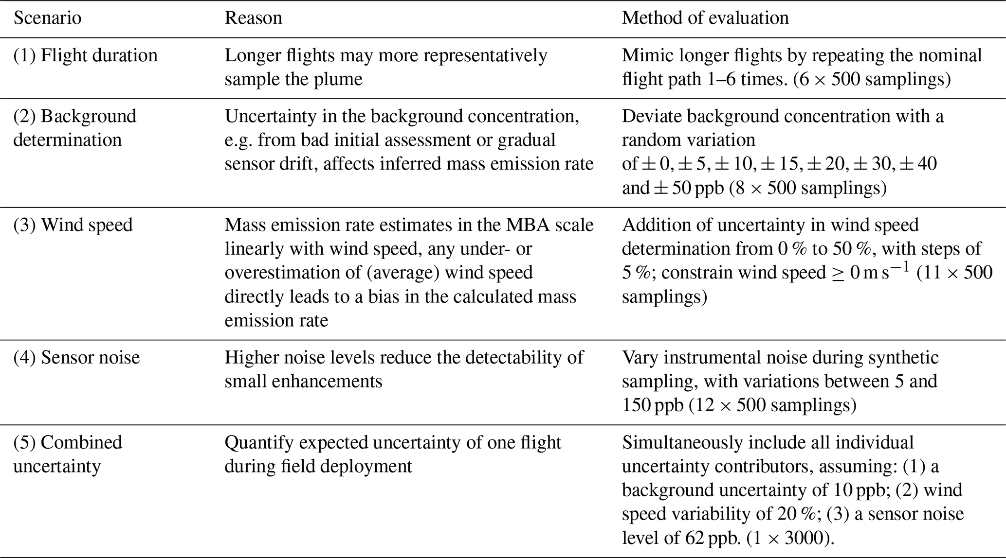
Table 2 lists the uncertainty contributors considered during this study, and the evaluation method in our OU-model. This uncertainty analysis allowed for a systematic evaluation of how individual and combined uncertainty sources propagate into UAS-based mass emission rate estimates, revealing the relative influence of each contributor. The setup for scenario 5 is based on parameter estimates from field campaigns and observations.

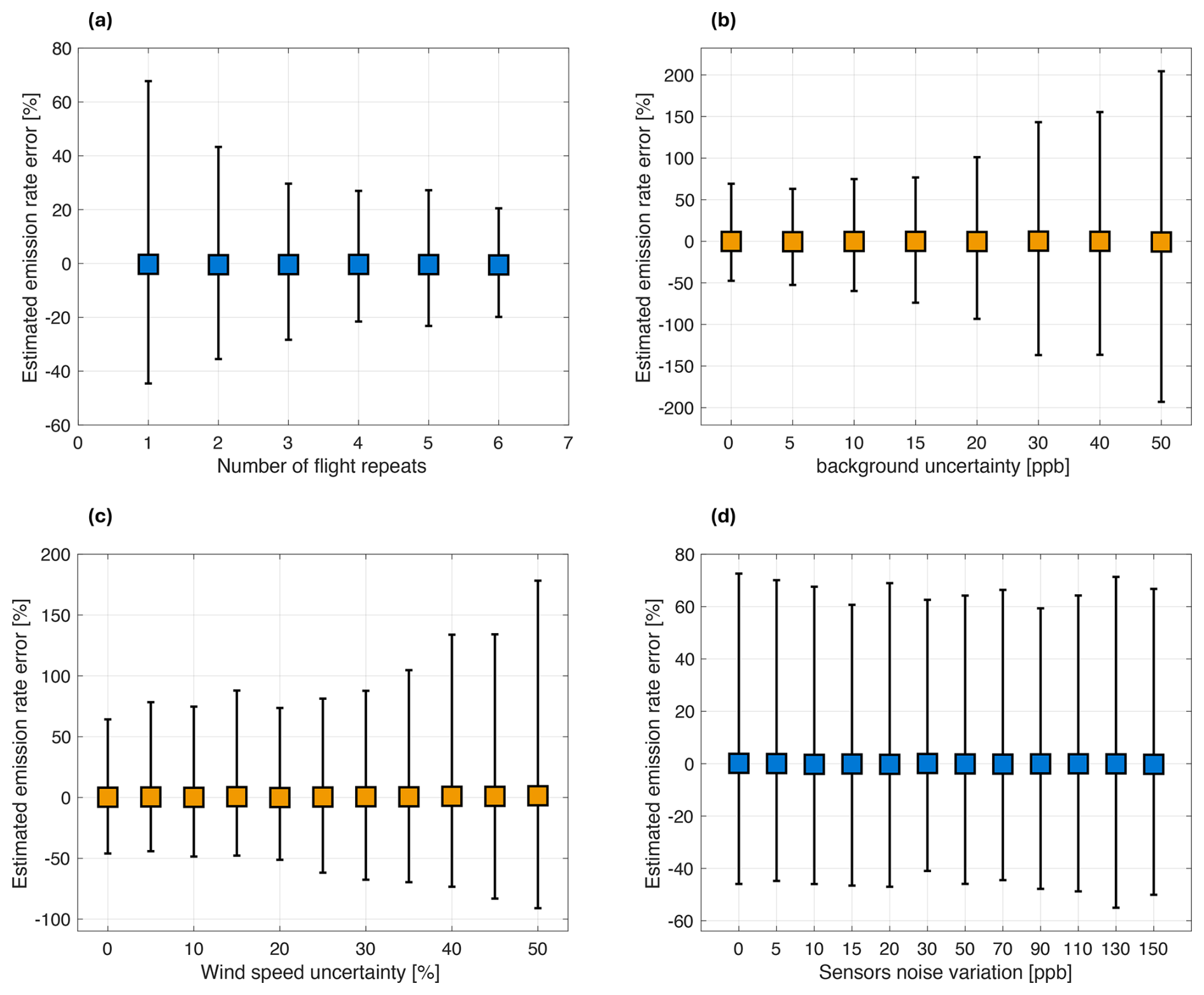
Figure 4 The marker shows the mean error, and the error bars present the 95 % confidence interval. (a) An overview of the mass emission rate estimates and the variability from 500 repeat simulations with an increase in number of flights. (b) An overview of the uncertainties linked to the background determination. (c) An overview of the mass emission rate estimates and the effect of the wind speed uncertainty. (d) An overview of the uncertainties linked to the instrumental noise.

4.2.1 Flight duration

Figure 4a shows how the standard deviation between the 500 modelled flights decreases with increasing duration of each flight. As expected, the results indicate that uncertainty decreases with longer (or multiple) flights, increasing the probability of representatively quantifying the full plume. With only a single flight (∼ 12 min), the mean mass emission rate is 10.3 kgCH₄ h⁻¹ [5.5–16.7 kgCH₄ h⁻¹; 95 % CI]. Increasing the flight duration lowers the CI bounds and the standard deviation (Scheutz et al., 2025), with the standard deviation decreasing from 27 % (1σ) for one flight to 15 % for three flights [7.5–13.6 kgCH₄ h⁻¹] and reaching its minimum of 11 % for six flights [8.4–12.7 kgCH₄ h⁻¹].

Increased flight duration decreases the CI of the mass emission rate estimates, as depicted in Fig. 4a. One flight per source increases the possibility of reporting an over- or under-representation of the total mass emission rate. With short flights (or a low number of flights), atmospheric stochasticity has a larger impact. Increasing the number of flights and averaging the resulting estimates offset this concern. With more flights, flights are conducted across a wide range of conditions, increasing the likelihood of representatively quantifying the plume. Our finding that repeated sampling of the same plume improves rather than increases the estimate of the mass emission rate makes intuitive sense. With every individual pass, the UAS may miss or double encounter the plume. This stochasticity averages out over multiple flights as is illustrated in Appendix Fig. K2.

4.2.2 Uncertainty effects of background errors

As mentioned in Sect. 3.7, multiple techniques are available to determine the in-flight background concentrations. However, the assumptions underlying these techniques, e.g. spatial and temporal uniformity of the background, instrument precision and absence of drift or sufficient sampling outside the plume, may not always hold (Edwards et al., 2025). This introduces an additional source of uncertainty into mass emission rate measurements. Reliable background determination is essential for accurate mass emission rate quantification, as even minor discrepancies can introduce systematic errors and consequently bias mass emission rate estimates (Allen et al., 2019; Cambaliza et al., 2014, 2015).

Figure 4b shows the impact of the uncertainty in the background determination on the mass emission rate estimate. Each run calculated the mass emission rate using the MBA with a varying background concentration. The figure shows that the estimated emission error increases with increasing background uncertainty. A background uncertainty of 30 ppb results in an estimated mass emission rate of 10.2 kgCH₄ h⁻¹ ([−3.6–23.9 kgCH₄ h⁻¹; 95 % CI]), and a standard deviation of 70 % (1σ). Based on the standard error of the observed background in our flights, we expect to determine background concentrations with an uncertainty of ± 10 ppb. Assuming the uncertainty in the background to 0–10 ppb, constrains the standard deviation to below 35 % (1σ). However, we infer a high sensitivity of the inferred mass emission rate to errors in the assumed background. At ± 20 ppb uncertainty in the background the standard deviation exceeds 100 %, i.e., yielding a negative or double mass emission rate, underscoring the importance of accurate background concentration determinations.

4.2.3 Wind speed uncertainty

Wind speed uncertainties are known to introduce significant errors into mass emission rate estimates (Allen et al., 2019; Morales et al., 2022; Vinković et al., 2022). Figure 4c–d shows an overview of the simulation results for varying wind speeds (Fig. 4c) and instrumental noise (Fig. 4d).

Uncertainties in the wind speed profiles were generated by multiplying the expected logarithmic profile by its respective uncertainty, yielding unique wind profiles for each Monte Carlo realization, thus representing the situation where the true mean windspeed is different from what is assumed in subsequent calculations. Figure 4c shows the outcome of this analysis and the contribution of wind speed uncertainty to the overall mass emission rate errors. A low wind speed uncertainties (<10 %) limits the standard deviation to 30 % (1σ), and results in a mass emission rate estimate of 10.1 kgCH₄ h⁻¹ [5.0, 17.1 kgCH₄ h⁻¹; 95 % CI]. However, when the uncertainty increases, so does the standard deviation and the mass emission rate estimate. With a wind speed uncertainty of 50 %, the standard deviation of the determined mass emission rate exceeds 60 % (1σ), and the mass emission rate estimate becomes 9.7 kgCH₄ h⁻¹ [0.6–23.7 kgCH₄ h⁻¹; 95 % CI]. These findings highlight the importance of minimising the wind speed errors by obtaining reliable wind speed measurements during flights.

The results, showing an increase in the mass emission rate uncertainty with greater wind speed uncertainty, was expected. However, the finding contradicts Mohammadloo et al. (2025), who reported that mass emission rate estimates are unaffected by wind-speed variations because measured concentrations scale proportionally with wind speed. In principle, this is correct, since for a constant source strength, higher winds yield lower concentrations. However, this overlooks the impact of an erroneous wind speed on mass emission rate determinations. If the wind speed is underestimated (e.g. 3 m s⁻¹ instead of the true wind speed 4 m s⁻¹), the resulting mass emission rate will also be underestimated, since the mass emission rate scales proportionally with the wind speed.

4.2.4 Uncertainty effects of instrumental noise

High-frequency sensor noise makes it hard to accurately resolve brief spikes in CH₄, for instance during high-speed flights. To an extent this may be alleviated by reducing flight speed, at the expense of reducing plume coverage (for a given UAS endurance). Low-noise sensors enable improved detection of smaller plumes and enhance the spatial resolution of the nominal plume. Here, we mimic the effect of noise in the Monte Carlo simulation, applied by varying the noise levels added to the trace (time series) sampled from the simulated plume. The sensor's noise (at 2 Hz) was varied from 5 to 150 ppb, generically representing high-, to low-precision sensors. Figure 4d shows that increasing noise does not directly affect the estimated error, as random fluctuations largely cancel during spatial interpolation.

The main impact of changing sensor noise is on background determinations. High-precision sensors usually allow straightforward application of approaches such as the 10th percentile method, whereas higher-noise sensors require additional processing with typically less certain results. Without this processing, applying the 10th percentile method to noisier sensors will lead to an overestimation of the mass emission rate, since the enhancements will appear larger than they actually are.

4.2.5 Combined uncertainty

The individual uncertainty analyses provide valuable insights into the role of individual factors on the emission estimate. During field campaigns, these factors (among others) are expected to affect the mass emission rate quantification simultaneously. To assess their combined effect, all the above sources of uncertainty were analysed in a single MC simulation. These uncertainty contributors were set to values (Table 2) encountered during actual deployment.

This simulation was used to estimate the overall combined uncertainty during our field campaign for a single flight. With the above-mentioned setup, the obtained mass emission rate was 10.0 kgCH₄ h⁻¹ ([3.3–19.1 kgCH₄ h⁻¹; 95 % CI), with a standard deviation of ± 40 % (1σ). During field deployment, the variability of the observed plume was 39 % (1σ, n=4). The observed simulation uncertainties and the field example agree well. Furthermore, the main contributors to the uncertainty identified with the simulation are consistent with those reported in other studies (Andersen et al., 2021; Karion et al., 2013; Morales et al., 2022; Nathan et al., 2015). To the point of our study sensor noise does not emerge from the uncertainty analysis as dominant.

4.2.6 Summary

This statistical analysis covered a range of potential sources of uncertainty to elucidate their expected contribution to the mass emission rate estimates. Table 3 provides an overview of the uncertainty sources discussed and their effects on the standard deviation, from the nominal scenario to the most considerable impact. Table 3 highlights that the background uncertainty and the wind speed uncertainty have the highest impact on the uncertainty of the estimate of the mass emission rate. Sensor noise is determined to not be a meaningful factor, especially when other uncertainties are more substantial (depicted in Table 3).

Table 3 Summary of the influence of various sources of uncertainty.

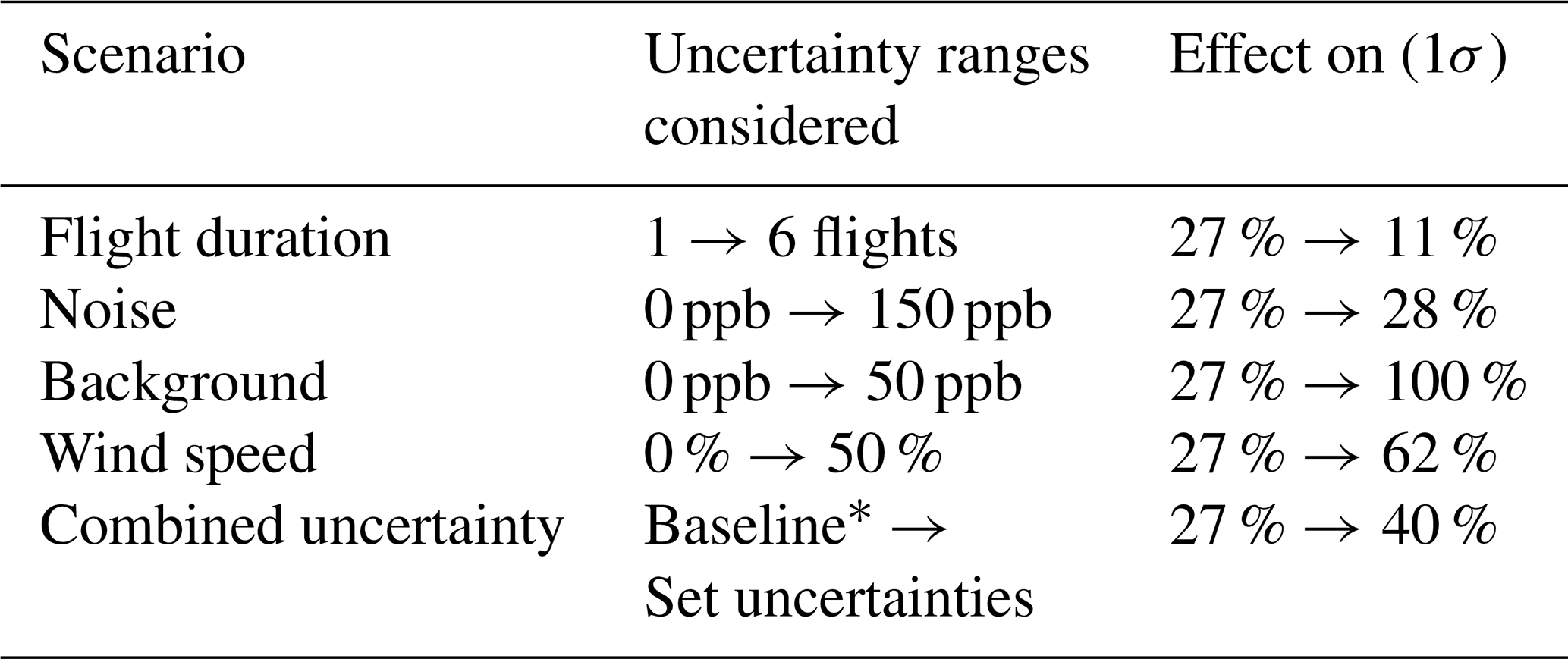
^∗ Baseline describes the lowest possible value (e.g. no variability or noise).

4.3 Applicability to various source strengths

During the uncertainty analysis, the influence of individual sources was evaluated for a reference emission rate of 10 kgCH₄ h⁻¹. In practice, emission rates can vary widely depending on source type and environmental conditions, and the relative importance of different uncertainty sources depends strongly on the source strength. Most importantly, the background uncertainty and sensors noise may become too large to derive a meaningful mass emission rate. To assess this relationship, we repeated the analysis in Sect. 4.2.5 for source strengths ranging from 1 to 20 kgCH₄ h⁻¹ and performing 1–6 flights using 500 MC realizations each. The results are summarized in Fig. 5.

Figure 5 shows that multiple flights reduce relative uncertainty. At lower emission rates, mass emission rate estimates are more susceptible to instrumental errors, where noise and background uncertainties are dominant factors (Appendix L). These random errors are effectively averaged out through repeated sampling. In contrast, estimates of larger emission rates are less influenced by sensor performance and are instead dominated by meteorological errors. As these errors are not reducible through averaging, multiple flights result in a persistent uncertainty of approximately 20 % (1σ).

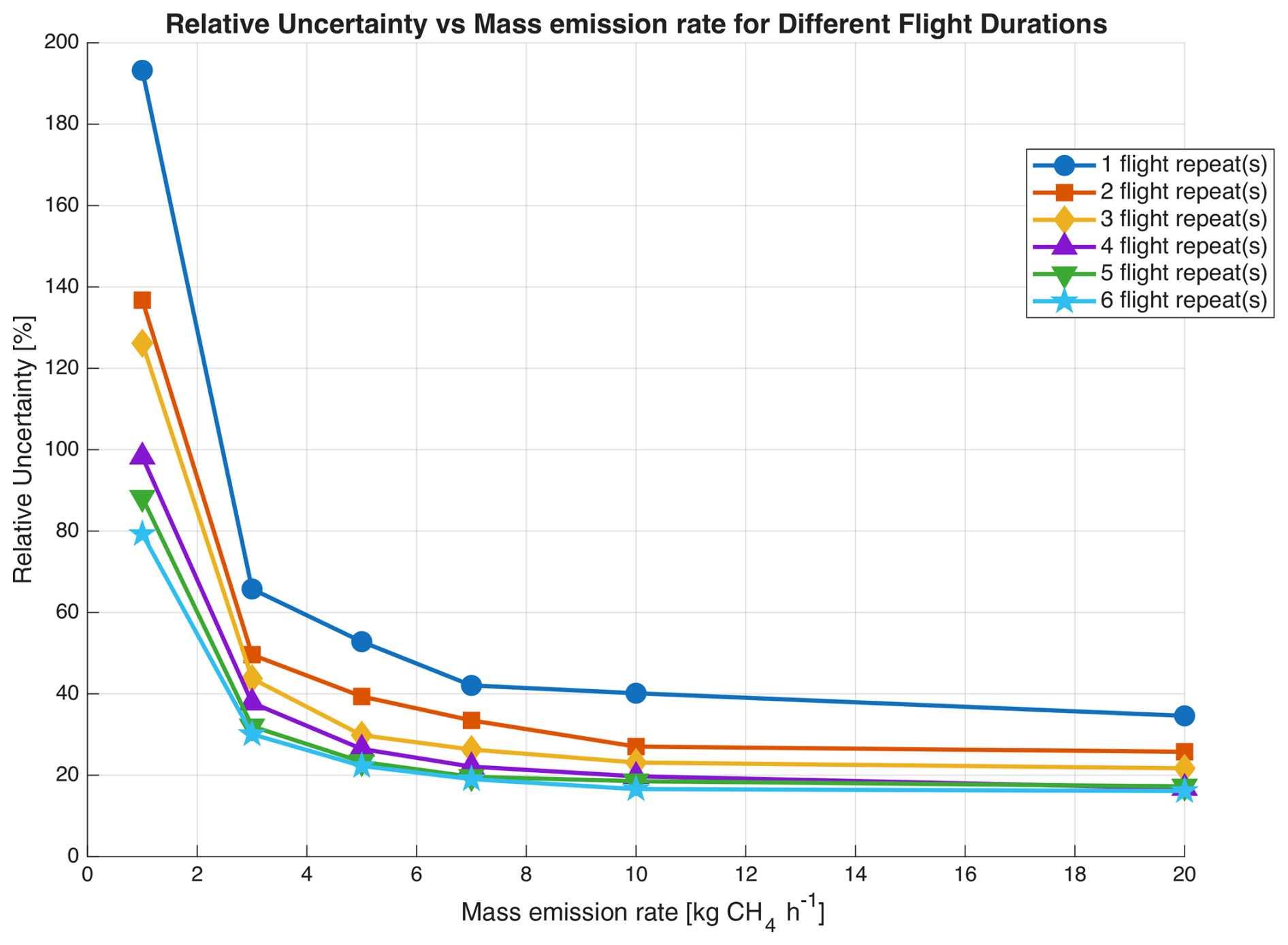
Figure 5 Relative uncertainty in mass emission rate estimates for emission rates of 1–20 kgCH₄ h⁻¹ across an increasing number of flights.

5 Discussion

This study evaluated the performance of a cost-effective CH₄ sensor and demonstrated that it can provide mass emission rate estimates comparable to those obtained with a higher-precision UAS-based instrument (i.e. Active AirCore). Field validation showed that the cost-effective sensor produced mass emission rate estimates that differed <10 % from those obtained by the Active AirCore method. Results from the Active AirCore technique have a standard deviation of 26 % (1σ), while that of the Axetris is 39 % (1σ). This uncertainty is a combination of systematic errors, random errors in wind-related uncertainties, background uncertainties and variability in the actual mass emission rate.

The differences in the standard deviation of all flights indicate that, for the assessed farm mass emission rate of ∼ 4 gCH₄ s⁻¹, total uncertainty associated with our UAS-based mass emission rate estimates are influenced more by uncertainties in wind variability and plume sampling methods than by the precision of the employed cost-effective sensor. With a controlled cell temperature, the Axetris mass emission rate estimates are withing 10 % of the AirCore findings. The total uncertainty, which is 39 % (1σ), falls within uncertainty ranges reported by other UAS-based studies (Andersen et al., 2021; Karion et al., 2013; Morales et al., 2022; Nathan et al., 2015) using higher precision and accuracy sensors. However, it should be noted that the source and the meteorological conditions during these other studies are not comparable to this study.

The necessity of the temperature control is well illustrated by Flight 3 (Appendix J), which showed the impact on Axetris CH₄ readings of (strong) cell temperature drift. The drift occurred as a result of faulty PID control: the sensor accidentally warmed prior to flight, which was caught, and thus cooled during flight, see Fig. A2. This clear drift of the measurement baseline, and an apparent oscillation around that (see data at 13:14; Fig. J2) hinders the assessment of the background CH₄ and thus to infer a meaningful mass emission rate.

Furthermore, this study highlights that improving post-flight data processing and obtaining accurate in situ meteorological observations are most important for reducing UAS-based uncertainties. These findings are consistent with previous studies that identify wind speed and direction as dominant sources of uncertainty in UAS-based CH₄ mass emission rate estimation (Morales et al., 2022; Yong et al., 2024; Mohammadloo et al., 2025; Wietzel et al., 2025). Wind-related errors are difficult to mitigate and can propagate non-linearly through the MB calculation, as a combination of wind direction and wind speed uncertainties. Background concentration uncertainty can typically be reduced through sufficient downwind sampling. Especially, small source strengths are influenced by background uncertainty, since the enhancements are usually small. Yong et al. (2024) noted that background variation accounted for only 6 % of the total uncertainty, with a strong source. The uncertainty found in this study, showed a larger uncertainty with smaller source strengths, indicating that sources with considerable enhancements are less influenced by a 10 ppb change in background concentrations.

The statistical analysis provides insight into potential sources of uncertainty in UAS-based sampling. The OU-simulation is appropriate for the specific flight trajectory presented in this study. The uncertainties derived using the simulation remain reasonable when real-world flights are conducted comparable to those simulated. Deviations may arise when observed mass emission rates are highly variable over a short time (i.e. one hour) or when the flight path (specifically: sampling density) is sparser than the modelled configuration. In those cases, the simulation results may no longer be representative. Flight paths of all flights in this study are comparable to flight 1, therefore OU-derived uncertainties can be applied to all flights.

However, not all sources of uncertainty have been considered. First, this study did not include the effects of spatial sampling density, which can also affect the accuracy of the mass emission rate measurements. Significant data gaps negatively affect the MBA, leading to systematic underestimation of the mass emission rate. This limitation has been addressed in detail by Mohammadloo et al. (2025). Higher-frequency observations in the horizontal and vertical directions decrease the estimated emission rate error. Based on their findings and our own flight track featuring relatively dense horizontal and vertical coverage, we expect to have only an additional 5-10 % error. Furthermore, wind direction uncertainties are also not included in the statistical analysis. Changes in wind direction influence the dispersion and detection of atmospheric plumes and is often referred to as the meandering effect (Wietzel et al., 2025). As mentioned before, wind variability (e.g. changed in wind speed and wind direction) propagate non-linearly through the MB calculations, therefore affecting the mass emission rate estimates in varying ways, depending on the error. Future work should combine optimised flight-path design with real-time plume detection to further minimise spatial sampling bias.

Our flight strategy provided abundant sampling with multiple transects at varying altitudes, creating favourable conditions for both IGA and MBA. Andersen et al. (2021) studied mass emission rates from coal-ventilation shafts using both methods and showed higher uncertainties for the MBA (26 %–51 %), compared to the IGA (8 %–16 %). In their research, the MBA uncertainty is dominated by wind speed. The IGA uncertainty reflects the standard error derived from 1000 optimisation iterations. Kim et al. (2023) also mention that the IGA is less sensitive to undersampling of plumes and upwind background levels, but the method can be considerably influenced by atmospheric stability.

Wind direction during the flights was variable, leading to a horizontally stochastic plume observations, making appropriate the use of a method that does not rely on Gaussian plume assumptions. The analysis from Andersen et al. (2021) underscores the importance of multiple transects at different altitudes, and that the IGA performed best when the vertical spacing and the distance were smaller than 2.5 times the vertical distribution (σ_z) of the plume. Given that our sampling was abundant but accompanied by temporally varying winds, we employed only the MBA, as it remains valid without requiring a stable Gaussian plume structure and provides a transparent, wind-driven uncertainty estimate.

Overall, the findings highlight that the implementation of cost-effective sensors offers a promising way to expand the spatial and temporal coverage of regional CH₄ monitoring. This scalability can improve emission quantification across a variety of sources, such as landfills, farms, and wastewater treatment plants. Besides, the sensor's effectiveness can be further improved when used as a stand-alone, since flight duration and number of flights increase due to a lower payload and less post-flight processing. The study reiterates that to maximise effectiveness, standardised flight procedures are required, together with precise background assessment and accurate meteorological observations during flight. Future studies should concentrate on a systematic comparison between the Axetris and high-precision, high-frequency in situ instrument. Similar to this study, both sensors should be deployed simultaneously, to allow direct comparison to mass emission rate estimates using comparable data analytics. Furthermore, large-scale controlled release experiments could provide a quantitative assessment of the sensors' performance in mass emission rate quantification.

6 Conclusions

This study demonstrates the feasibility of using a cost-effective, medium-precision, in situ CH₄ sensor (referred to as the Axetris) on UASs for rapid emission assessment. Laboratory characterisation indicates that temperature fluctuations strongly affect this sensor's measurement stability, rendering it unreliable for this work unless appropriate mitigative measures are taken. We improved the sensor's performance by properly insulating the sensor and applying active thermal regulation to maintain a constant cell temperature (±0.05 °C). Adding active temperature control removes the unwanted measurement oscillations, maintaining the long-term accuracy of the Axetris even when bigger environmental temperature changes are present. Allan variation analysis confirmed that under stable laboratory conditions, the sensor achieves a precision of 63 ppb at 2 Hz and remains stable to within ± 10 ppb over a 20 min time scale. Insights gained from laboratory characterisation supported the preparation of the sensor for UAS-based field tests. With active temperature control, and observing large temperature differences, the sensor remains stable within ± 20 ppb over a 20 min time scale.

Field experiments at a dairy farm confirmed that the Axetris can deliver reliable CH₄ mass emission rate estimates, comparable to those obtained using the established Active AirCore technique. Across four flights, the mean mass emission rate derived from the Axetris measurements was 4.1±1.6 gCH₄ s⁻¹, while the AirCore measurements yielded a mass emission rate of 4.2 ± 1.1 gCH₄ s⁻¹. The close agreement between the techniques, despite using different background determination methods tailored to each technique, validates the use of the Axetris sensor for reliable mass emission rate quantification.

An uncertainty analysis using the Ornstein-Uhlenbeck approach to identify the dominant sources of uncertainty in UAS-based mass emission rate measurements show the noise of this sensor does not significantly impact the total uncertainty, particularly when emission sources have a sufficiently large source strength and plume coverage is sufficient in space and time. In contrast, realistic uncertainties in wind speed estimates (common at low wind speeds) can introduce errors in the mass emission rate exceeding 60 %. An accurate determination of background concentration is also important, since errors in background estimation can account for more than 100 % of the total uncertainty for a mass emission rate of 10 kgCH₄ h⁻¹, with even greater sensitivity when CH₄ enhancements are low. Overall, weaker emission sources are more affected by instrumental errors compared to stronger sources. Multiple flights help to reduce the uncertainty in the background determination and average the effects of variable wind speeds and direction, while systematic errors in the wind speed (e.g., the assumed profile) remain persistent.

This study underscores that careful laboratory testing and compensation for environmental temperature variability, can significantly improve the performance of medium-precision sensors for mass emission rate estimation. This supports the potential for deploying these cost-effective sensors on UAS systems for GHG monitoring, thereby helping to close data gaps in national inventories.

Appendix A: Overview of a conceptual sensor system classification

Table A1 A conceptual classification of low-, medium- and high-quality sensors and their associated platforms. The costs columns approximate costs for acquisition and per-day use of these systems. Sensor characteristics are, also, indicative only. Listed values are based on informed estimates and not derived from verified references and should be interpreted accordingly.

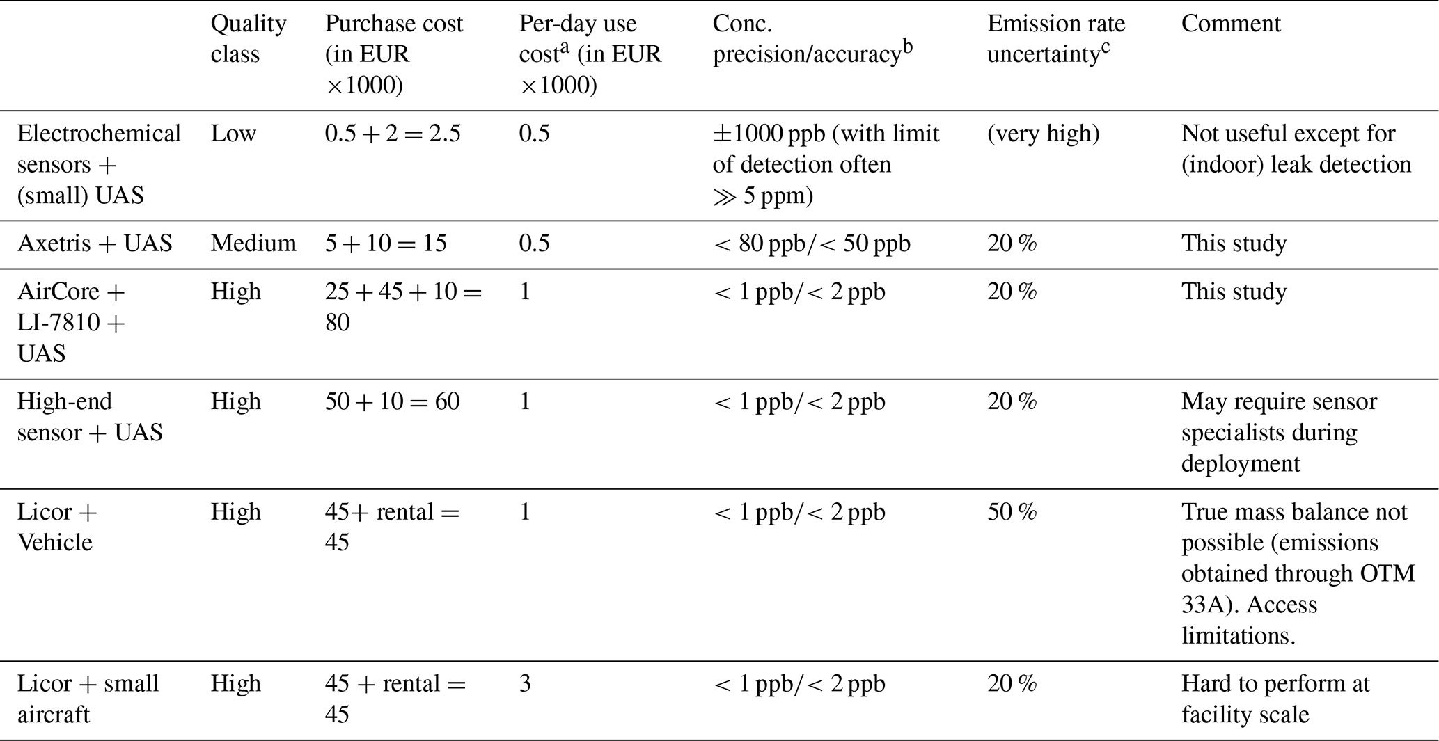
^a All high-quality class instruments are assumed to require two operators, while low and medium-class sensors are assumed to require one. Prices are based on salaries in Northern Europe. ^b Accuracy is operationally approximated here as the instrumental drift that may roughly be expected over the duration of an emissions quantification deployment (e.g., between calibrations/during a flight). This is <50 ppb for the Axetris (see Fig. 2 of the manuscript) and typically is much smaller for high-end sensors. Note that these figures are intended to indicate performance ranges, not precise technical specifications. ^c Emission uncertainties are based on their respective techniques and the best-case scenarios (i.e. when conditions are most optimal and fluxes are not variable).

Appendix B: Temperature control during flight

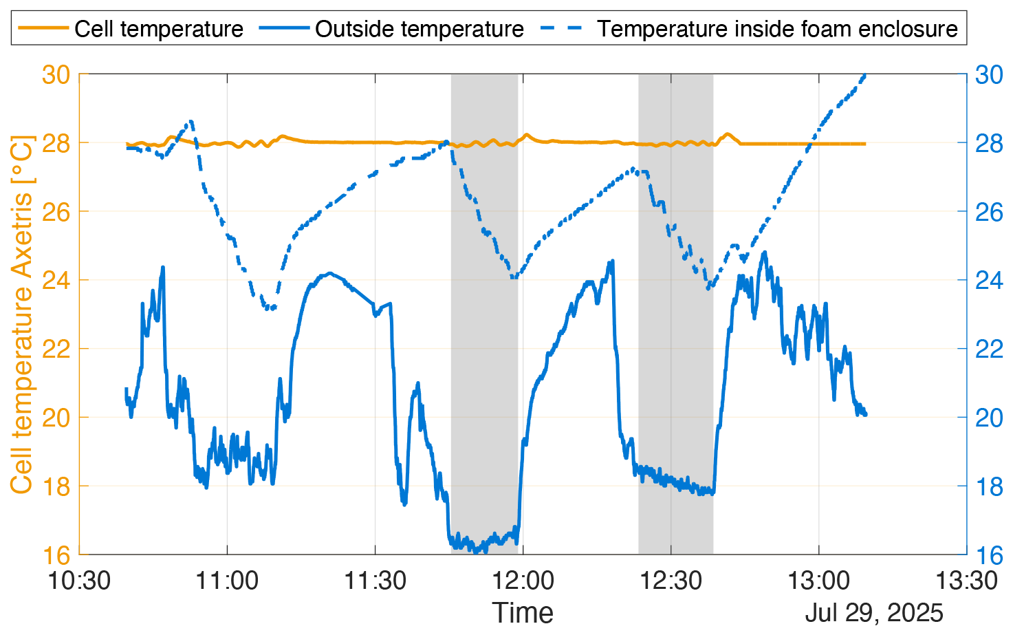
Figure B1 Temperature stability during flights one and two. The actively controlled temperature recorded by the Axetris sensor is shown in orange (left axis; set to 28 °C) The shaded regions indicate the flight periods. The solid blue line denotes the ambient air temperature (as measured on the package envelope), while the dashed blue line shows the temperature of the PCB of the Axetris inside the foam enclosure (right axis). Note the warming up of the system between flights, while out of the wind, and in occasional sunlight.

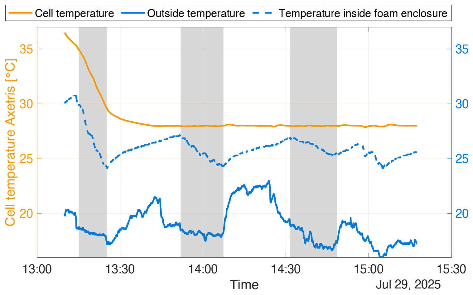
Figure B2 Same as Fig. B1, but for flights three, four and five. Prior to flight three, the Axetris was accidently heated to 36 °C. The rapid cooling during flight severely affected the Axetris stability.

Appendix C: Linearity test

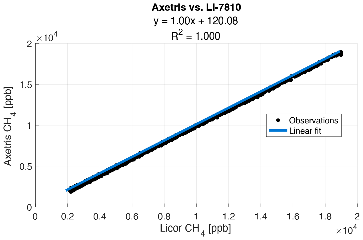
Figure C1 Linear regression plot showing the linearity between LI-7180 and Axetris data. The outliers are due to differences in response time.

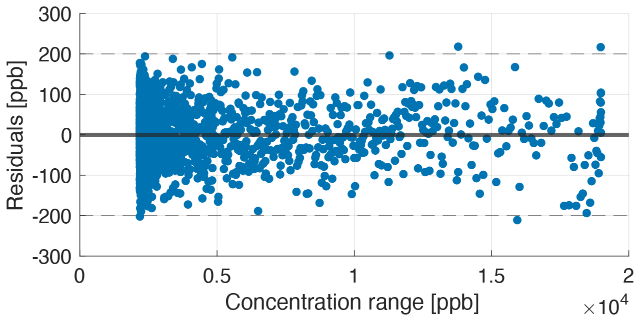
Figure C2 Residual plot of the linear regression model shown in Fig. C1, illustrating the residuals over the concentration range of 2 to 20 ppm. No structure is observed in the distribution of residuals along the range of concentrations, demonstrating that – as far as may be observed within the Axetris's noise – the linearity of the Axetris matches that of the LI-7810. Observed RMSE: 70 ppb.

Appendix D: Experimental setup of the water vapour test

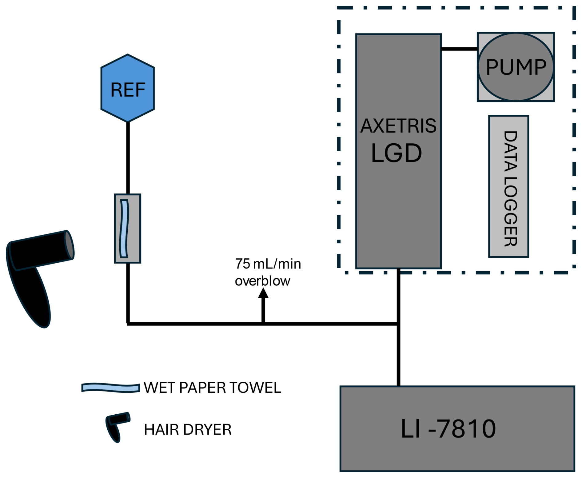
Figure D1 Overview of the water droplet test setup. A small, wet (but gradually drying) piece of paper is placed in an enclosed compartment, temporarily wetting the air coming from a compressed air cylinder containing either ∼ 2 or ∼ 81 ppm CH₄. The compartment can be heated, thereby briefly increasing the water vapour concentration in the gas stream.

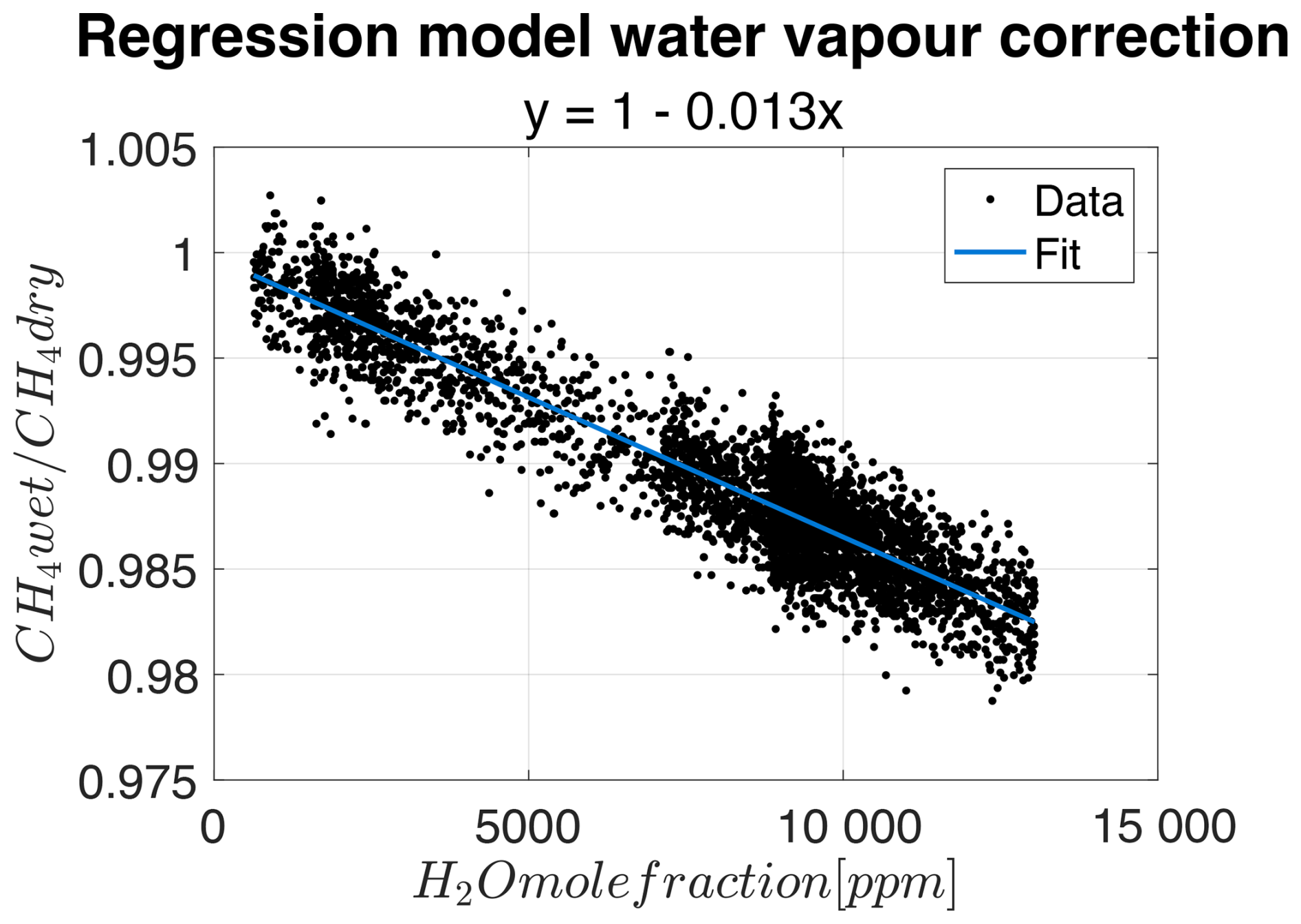
Figure D2 Regression model used to determine the water vapour correction as described in Sect. 2.4. The linear relationship between the wet and dry fractions is used to correct for water vapour during field experiments. Water vapour concentrations in this figure are obtained from the LI-7810. The R² value is 0.86.

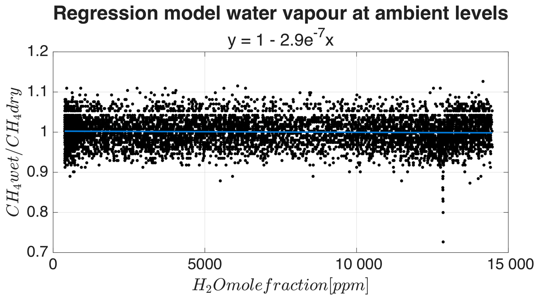
Figure D3 Regression analysis of the water vapour experiment under ambient conditions. At low ambient levels there is no significant relationship is observed.

Appendix E: System precision

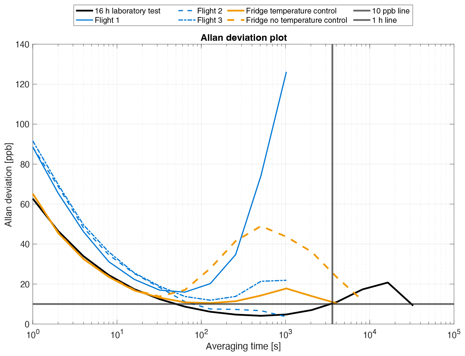
Figure E1 Visualization of the Allan deviation plot with additional lines showing the determination of hourly calibration.

Appendix F: Meteorological data

Figure F1 Wind rose of Windmaster pro observations during the campaign day at 29 July 2025.

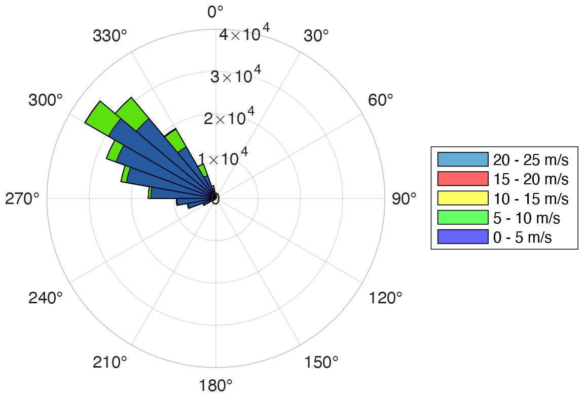
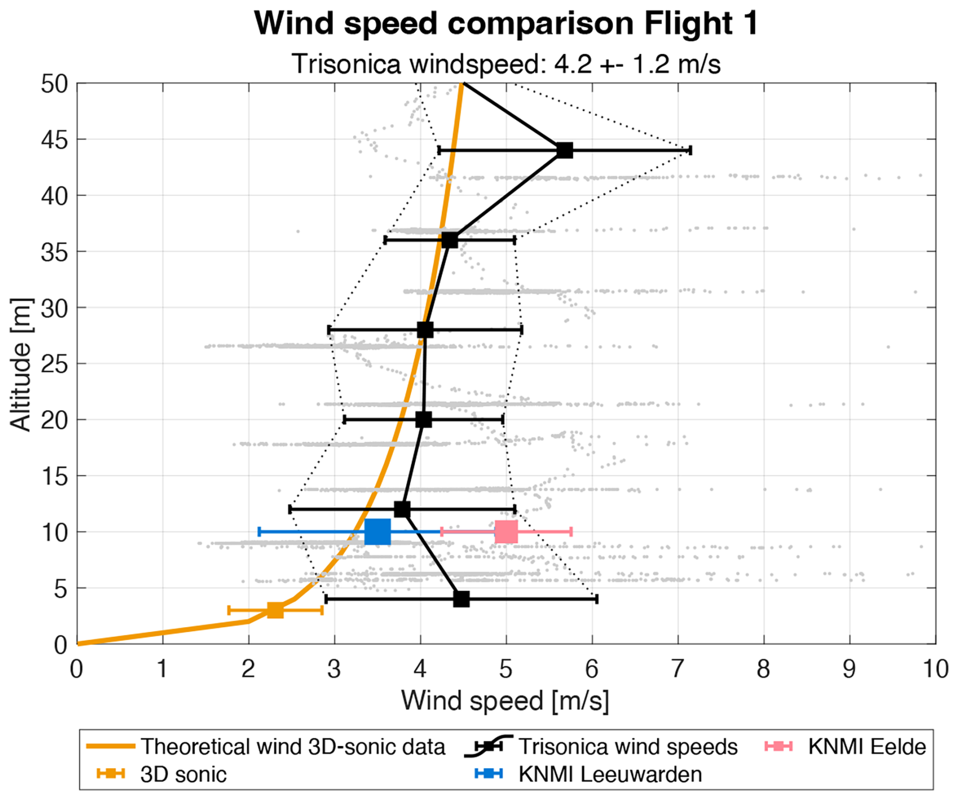
Figure F2 Compilation of wind speed information during Grijpskerk flight 1. Shown are a theoretical, exponential wind speed profile (orange line) anchored by measured data from the 3D sonic at 3 m altitude (orange marker) and the individual (light gray) and bin-averaged (black) TriSonica wind speed data collected by the UAS. The mean wind speed during flight observed by the TriSonica was 4.2 m s⁻¹ ± 1.2 m s⁻¹. Additional markers show KNMI observations from nearby stations Eelde (pink) and Leeuwarden (blue).

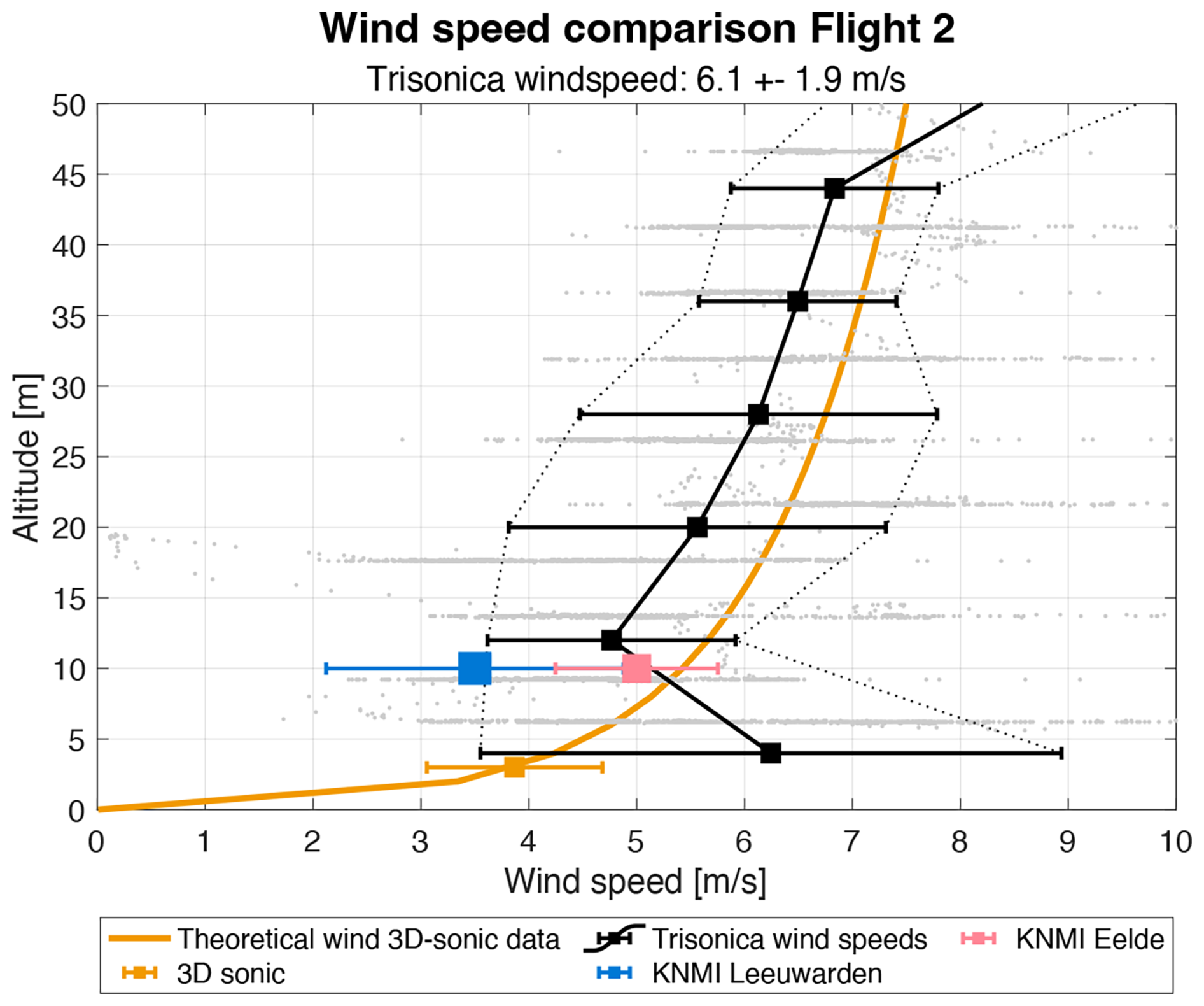
Figure F3 Compilation of wind speed information during Grijpskerk flight 2. Shown are a theoretical, exponential wind speed profile (orange line) anchored by measured data from the 3D sonic at 3 m altitude (orange marker) and the individual (light gray) and bin-averaged (black) TriSonica wind speed data collected by the UAS. The mean wind speed during flight observed by the TriSonica was 6.1 m s⁻¹ ± 1.9 m s⁻¹. Additional markers show KNMI observations from nearby stations Eelde (pink) and Leeuwarden (blue).

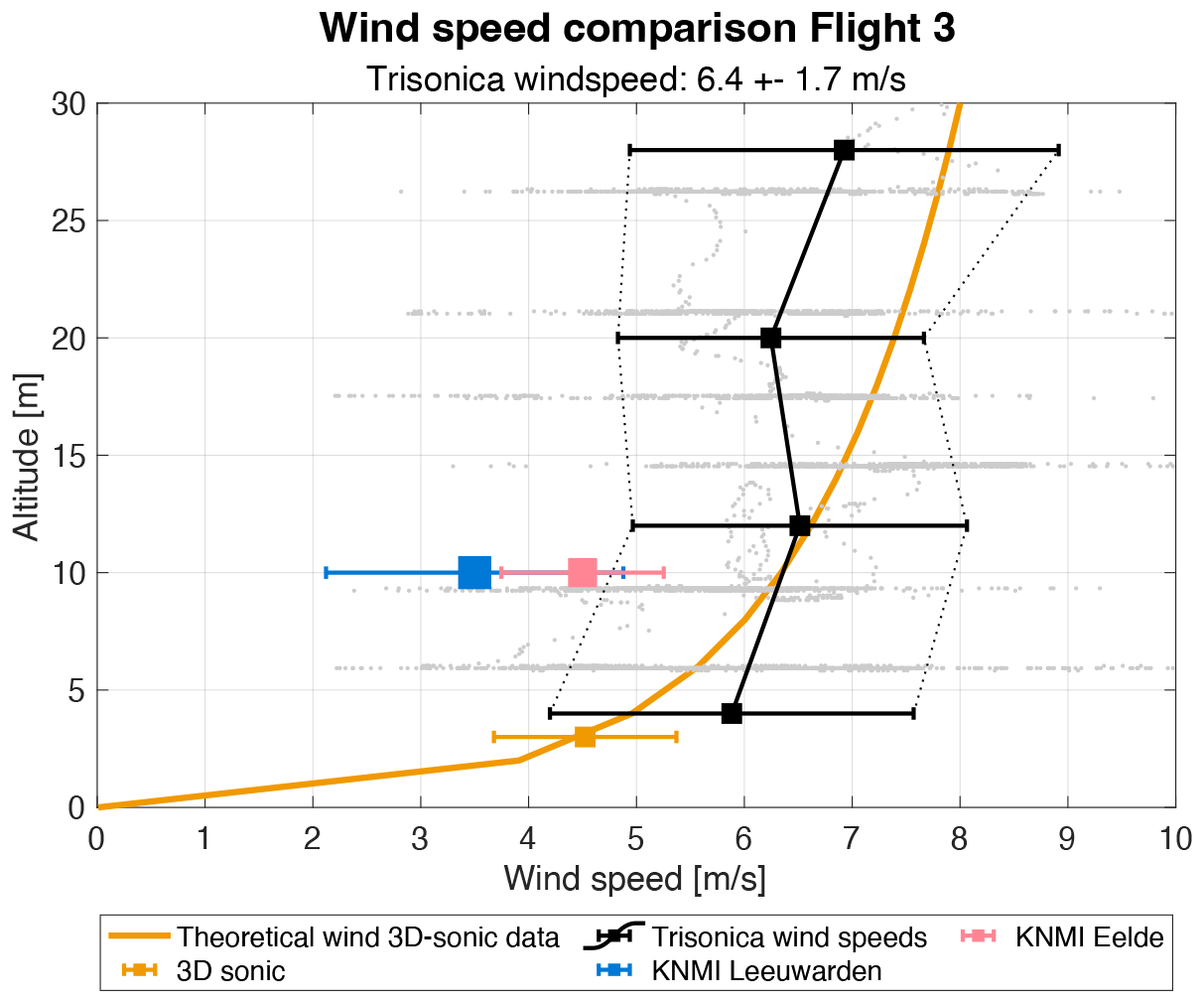
Figure F4 Compilation of wind speed information during Grijpskerk flight 3. Shown are a theoretical, exponential wind speed profile (orange line) anchored by measured data from the 3D sonic at 3 m altitude (orange marker) and the individual (light gray) and bin-averaged (black) TriSonica wind speed data collected by the UAS. The mean wind speed during flight observed by the TriSonica was 6.4 m s⁻¹ ± 1.7 m s⁻¹. Additional markers show KNMI observations from nearby stations Eelde (pink) and Leeuwarden (blue).

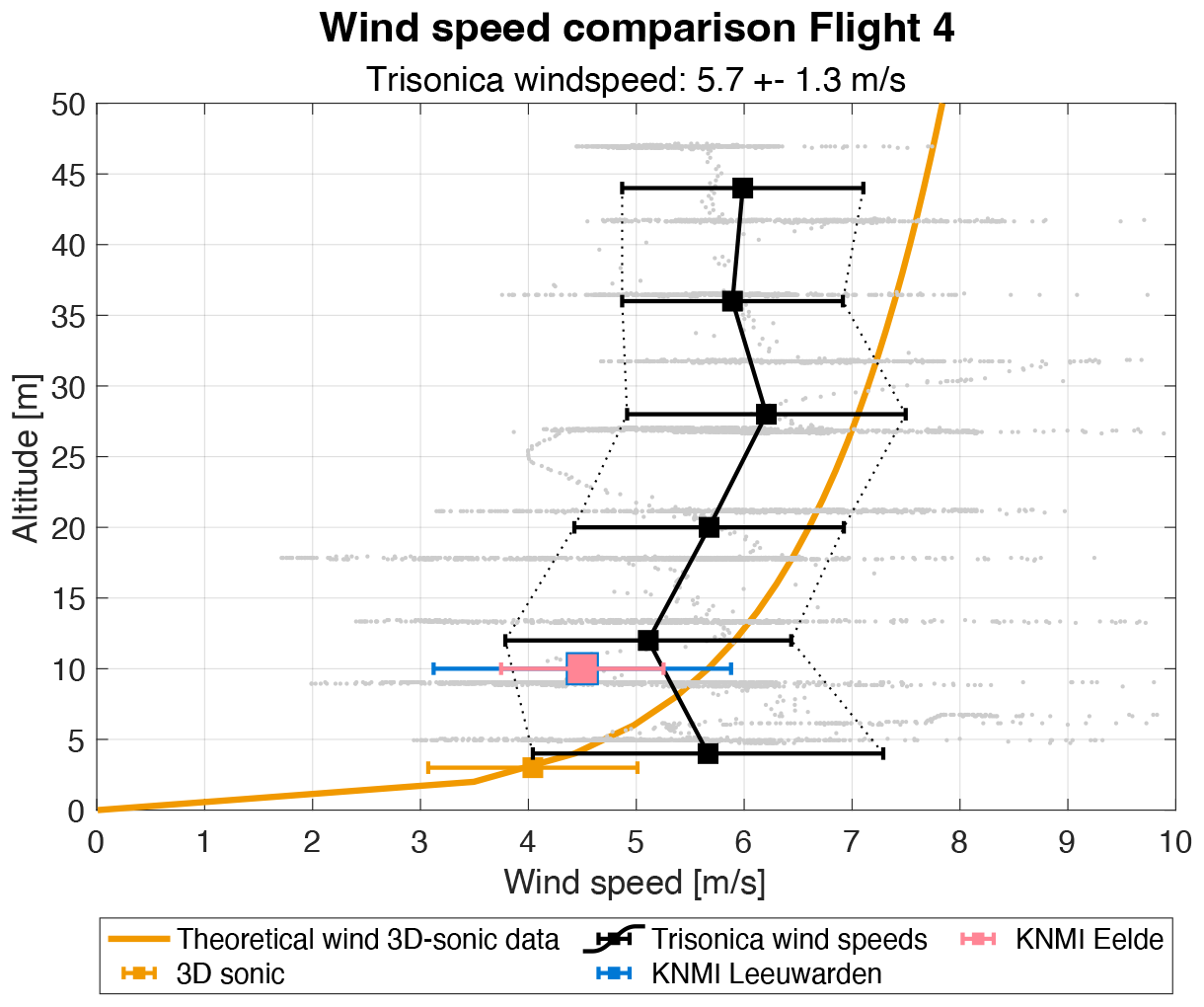
Figure F5 Compilation of wind speed information during Grijpskerk flight 4. Shown are a theoretical, exponential wind speed profile (orange line) anchored by measured data from the 3D sonic at 3 m altitude (orange marker) and the individual (light gray) and bin-averaged (black) TriSonica wind speed data collected by the UAS. The mean wind speed during flight observed by the TriSonica was 5.7 m s⁻¹ ± 1.3 m s⁻¹. Additional markers show KNMI observations from nearby stations Eelde (pink) and Leeuwarden (blue).

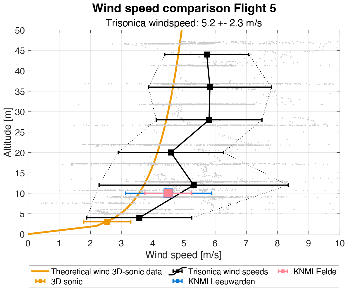
Figure F6 Compilation of wind speed information during Grijpskerk flight 5. Shown are a theoretical, exponential wind speed profile (orange line) anchored by measured data from the 3D sonic at 3 m altitude (orange marker) and the individual (light gray) and bin-averaged (black) TriSonica wind speed data collected by the UAS. The mean wind speed during flight observed by the TriSonica was 5.2 m s⁻¹ ± 2.3 m s⁻¹. Additional markers show KNMI observations from nearby stations Eelde (pink) and Leeuwarden (blue).

Appendix G: Background determination

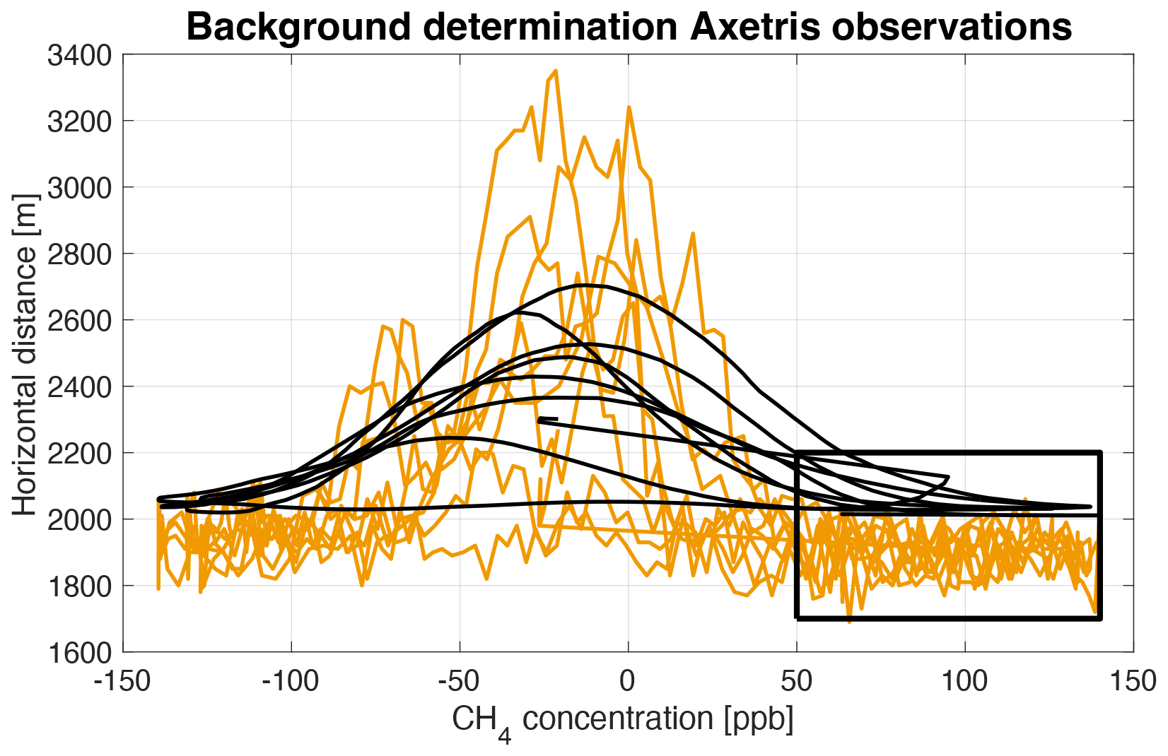
Figure G1 Method to determine the plume boundaries and background concentration of the Axetris observations (orange) and the AirCore observations (black) of flight 1. The enclosed area is thought to contain the background of the Axetris, and the average value is determined by isolating the specific observations.

Appendix H: Correlation Axetris vs. AirCore observations

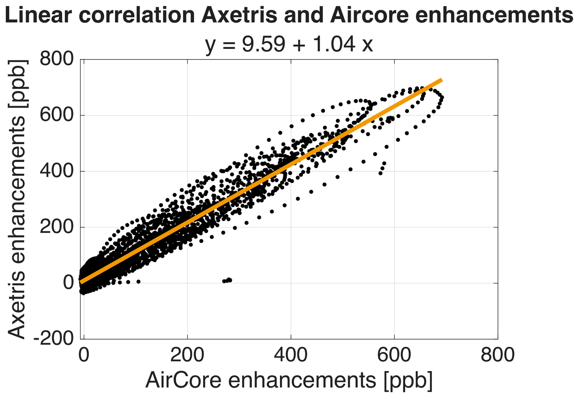
Figure H1 Linear correlation plot of the smoothed enhancements from Axetris observations compared to the enhancements measured by the active AirCore. All flight observations (with the exception of flight 3) are considered in this plot. The linear correlation coefficient is R²=0.94 and an RMSE of 36.5 is found.

Appendix I: Curtain orientation

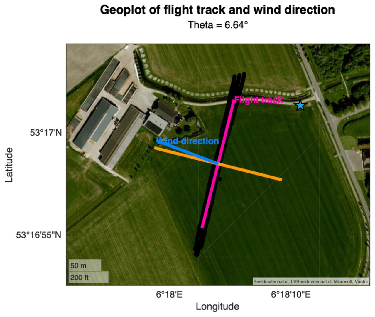
Figure I1 Top-down view of the flight track and CH₄ observations of the Axetris during flight 1. Figure used to determine the angular deviation between the perpendicular line (orange line) of the mean flight track (pink line) and the wind direction (blue). The blue star represents the position of the WindMaster Pro. Images: © Microsoft.

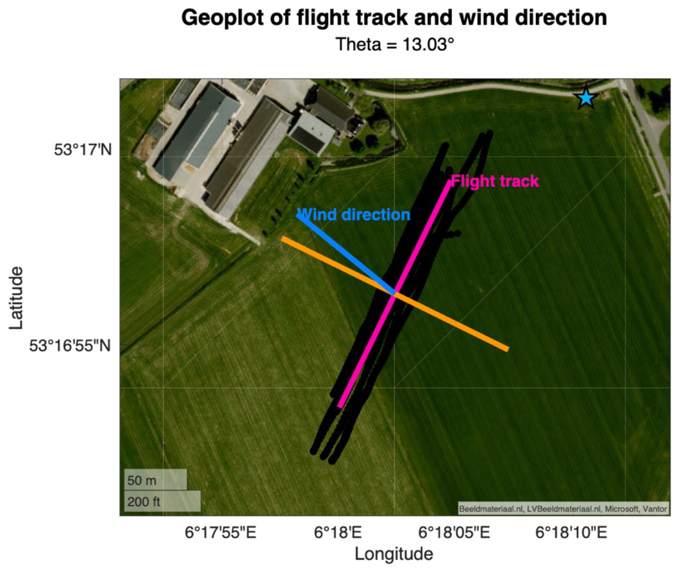
Figure I2 Top-down view of the flight track and CH₄ observations of the Axetris during flight 2. Figure used to determine the angular deviation between the perpendicular line (orange line) of the mean flight track (pink line) and the wind direction (blue). The blue star represents the position of the WindMaster Pro. Images: © Microsoft.

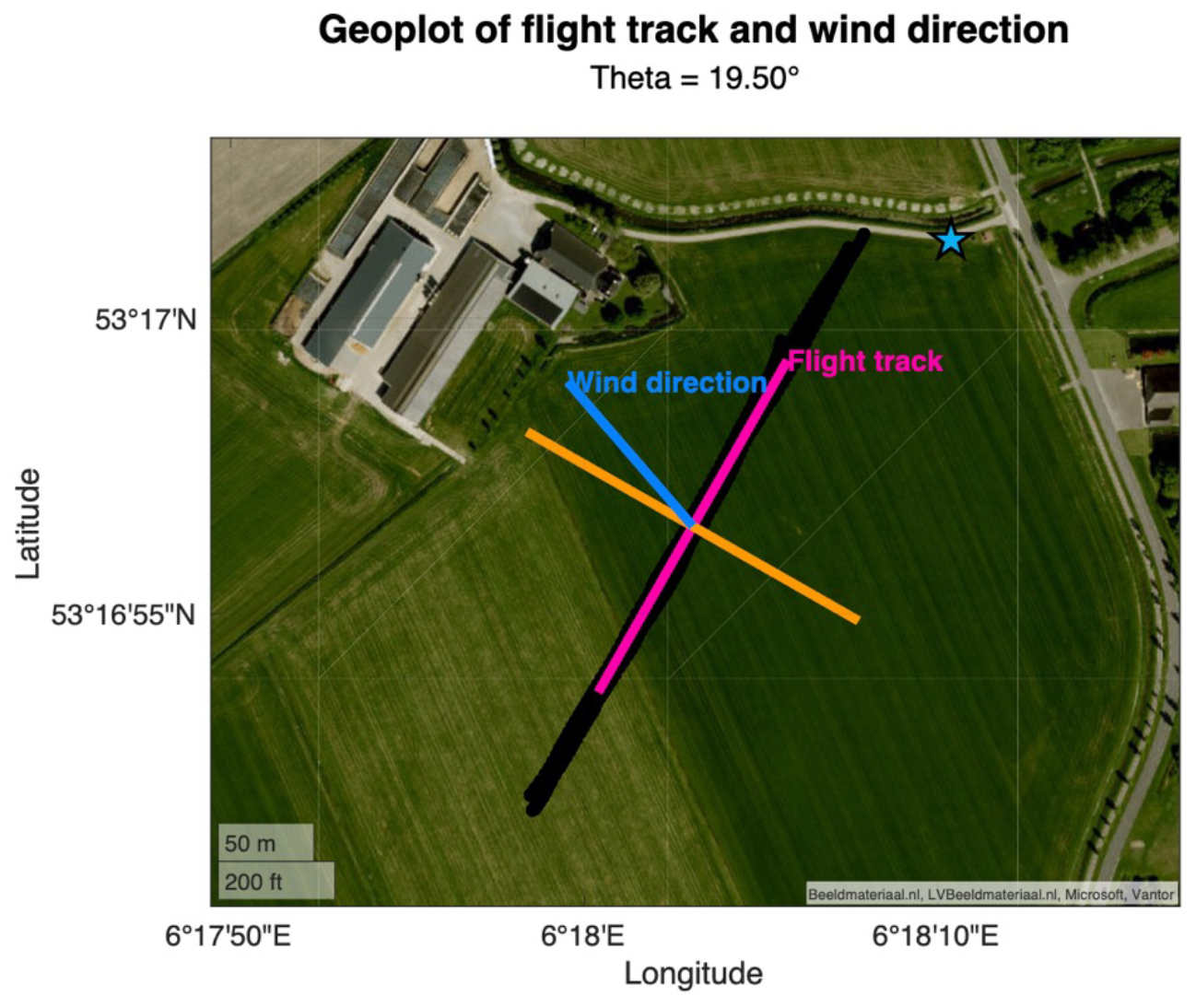
Figure I3 Top-down view of the flight track and CH₄ observations of the Axetris during flight 3. Figure used to determine the angular deviation between the perpendicular line (orange line) of the mean flight track (pink line) and the wind direction (blue). The blue star represents the position of the WindMaster Pro. Images: © Microsoft.

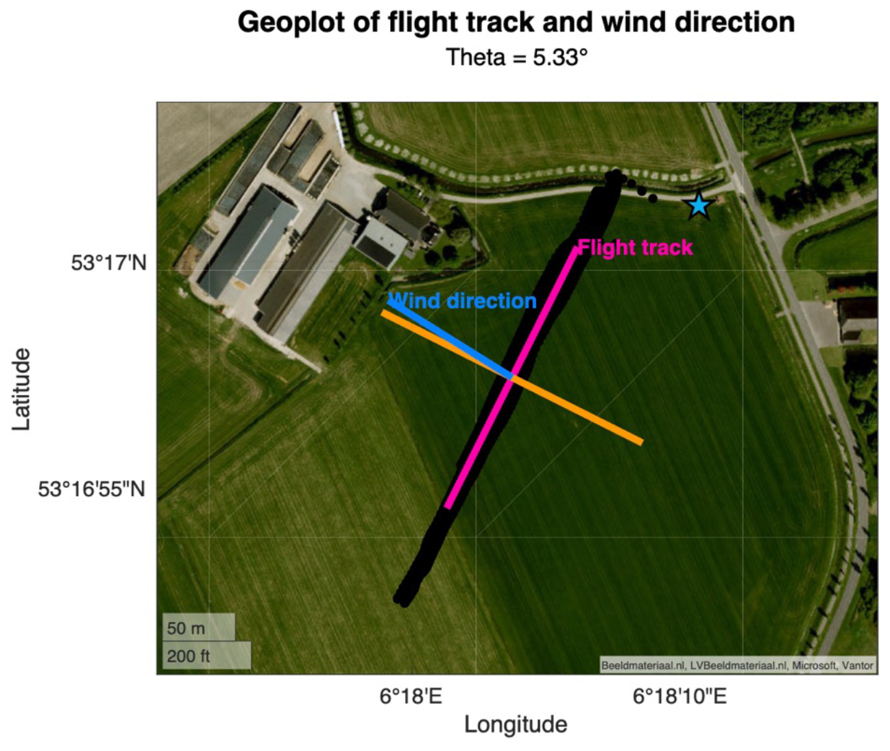
Figure I4 Top-down view of the flight track and CH₄ observations of the Axetris during flight 4. Figure used to determine the angular deviation between the perpendicular line (orange line) of the mean flight track (pink line) and the wind direction (blue). The blue star represents the position of the WindMaster Pro. Images: © Microsoft.

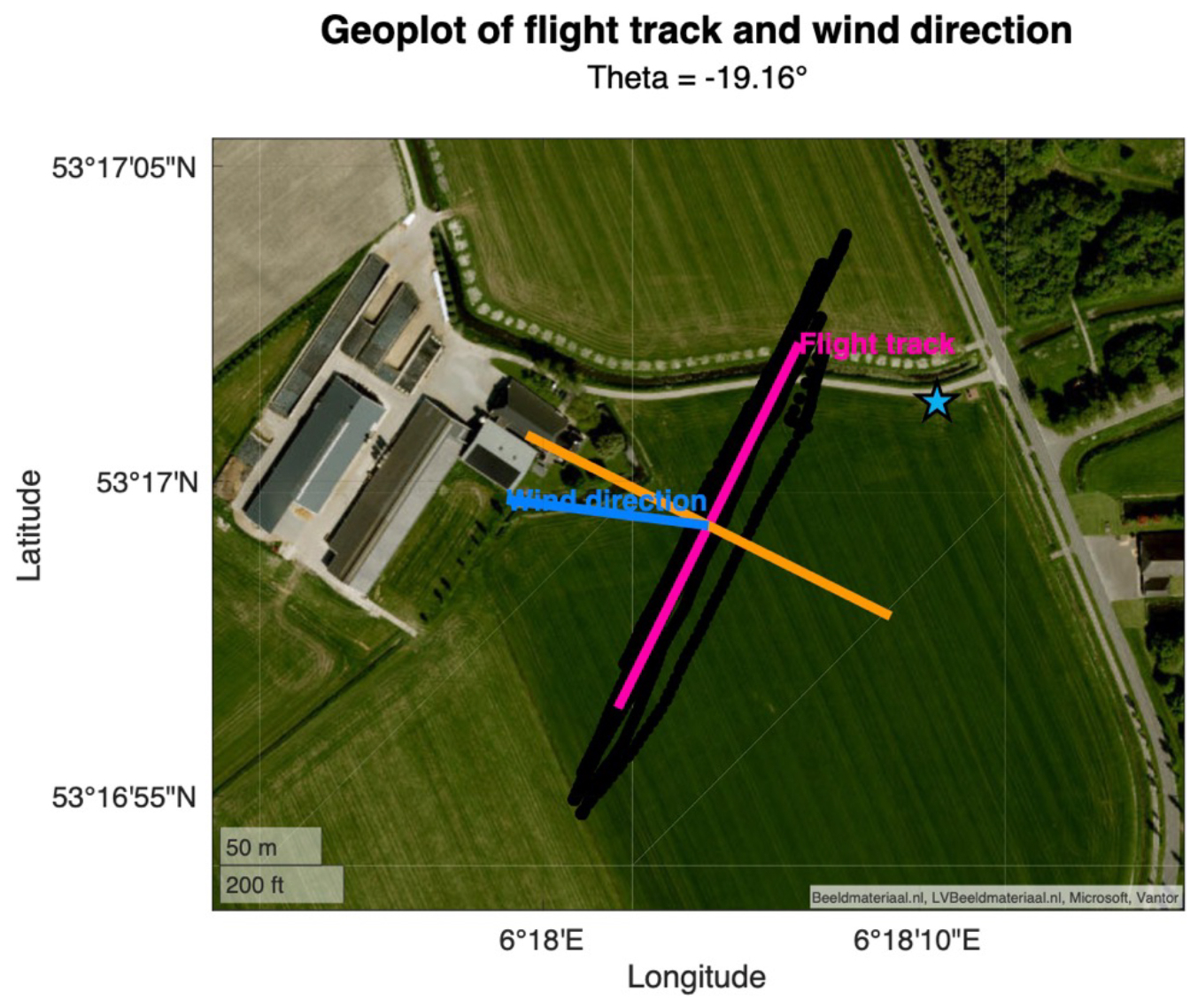
Figure I5 Top-down view of the flight track and CH₄ observations of the Axetris during flight 5. Figure used to determine the angular deviation between the perpendicular line (orange line) of the mean flight track (pink line) and the wind direction (blue). The blue star represents the position of the WindMaster Pro. Images: © Microsoft.

Appendix J: All flight profiles

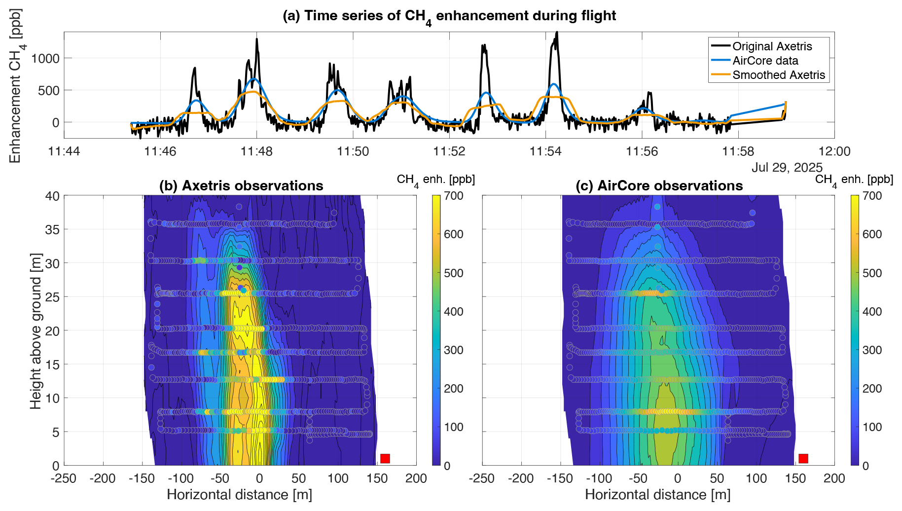
Figure J1 Overview of the observed CH₄ enhancements and spatial interpolation of flight 1. Estimated mass emission rate of Axetris 2.8 gCH₄ s⁻¹ (b); AirCore 3.5 gCH₄ s⁻¹ (c).

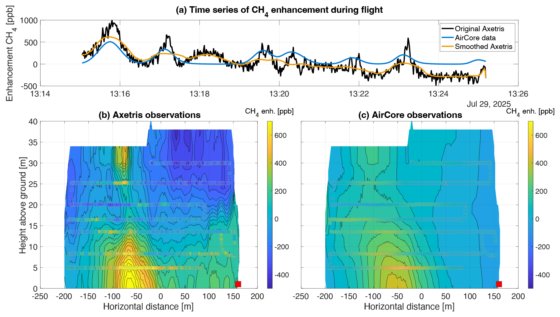
Figure J2 Overview of the observed CH₄ enhancements and spatial interpolation of flight 3. During the flight, the temperature control malfunctioned. This flight was left entirely out of the analysis.

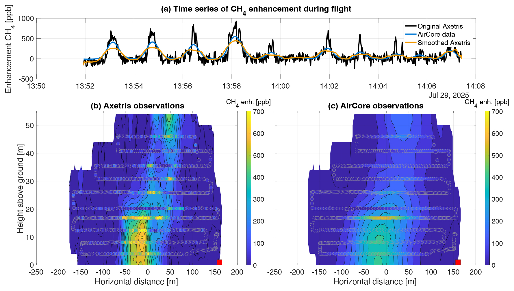
Figure J3 Overview of the observed CH₄ enhancements and spatial interpolation of flight 4. Estimated mass emission rate of Axetris 5.4 gCH₄ s⁻¹ (b); AirCore 5.0 gCH₄ s⁻¹ (c).

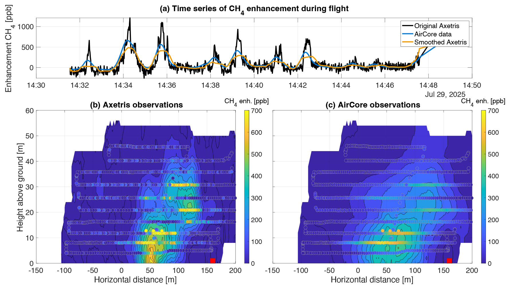
Figure J4 Overview of the observed CH₄ enhancements and spatial interpolation of flight 5. Estimated mass emission rate of Axetris 2.8 gCH₄ s⁻¹ (b); AirCore 3.0 gCH₄ s⁻¹ (c).

Appendix K: Plume simulation results

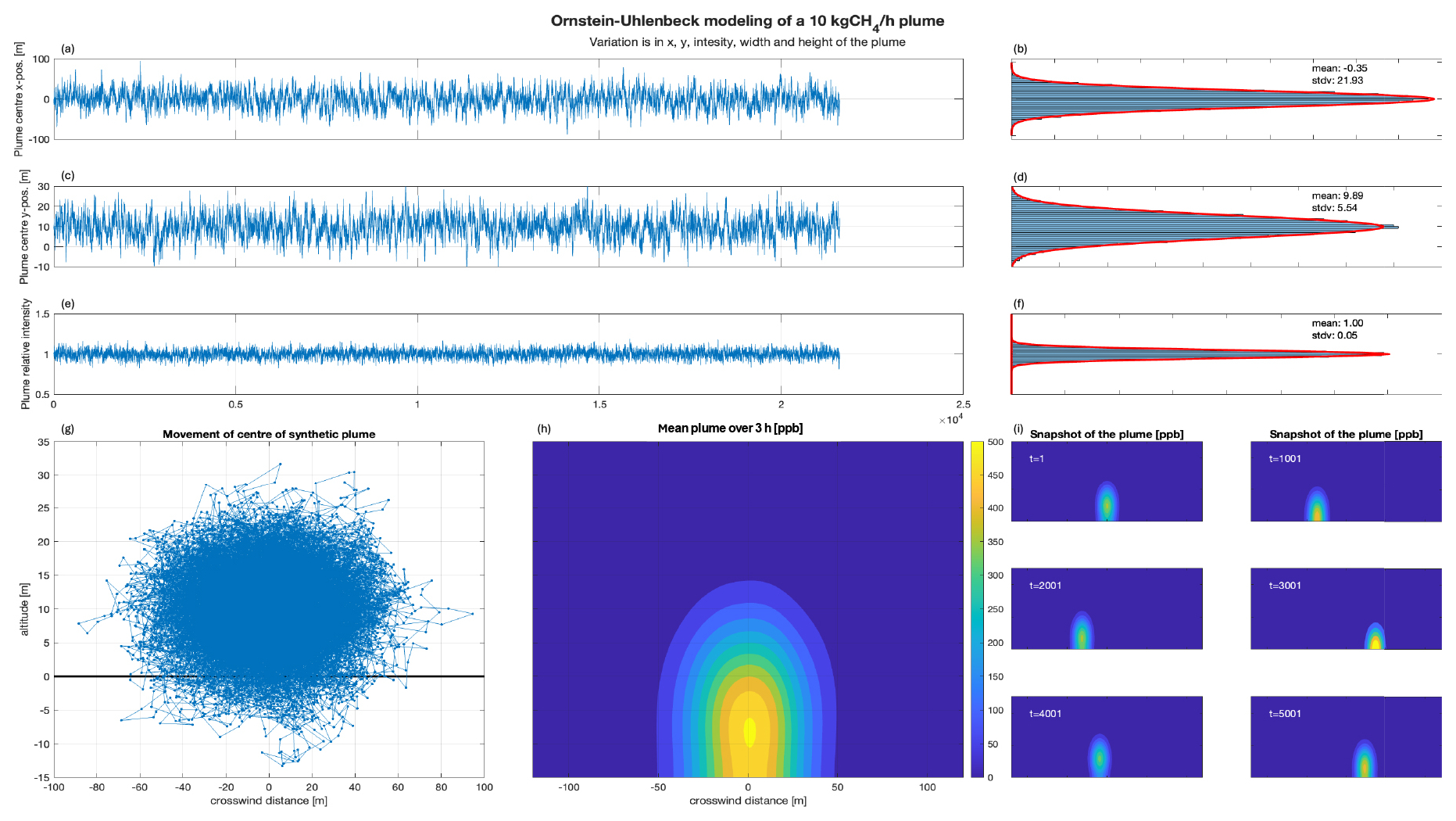
Figure K1 Stochastic plume simulation using the Ornstein-Uhlenbeck model to simulate a plume of 10 kgCH₄ h⁻¹. The top three figures (a–f) depict the time series fluctuations of the plumes horizontal and vertical position and plume intensity and spread are presented, together with the probability distribution of these parameters; (g) The simulated trajectory of the plume around the centerline motion; (h) the spatial interpolation of the 3 hour averaged plume; (i) example of instantaneous plume snapshots.

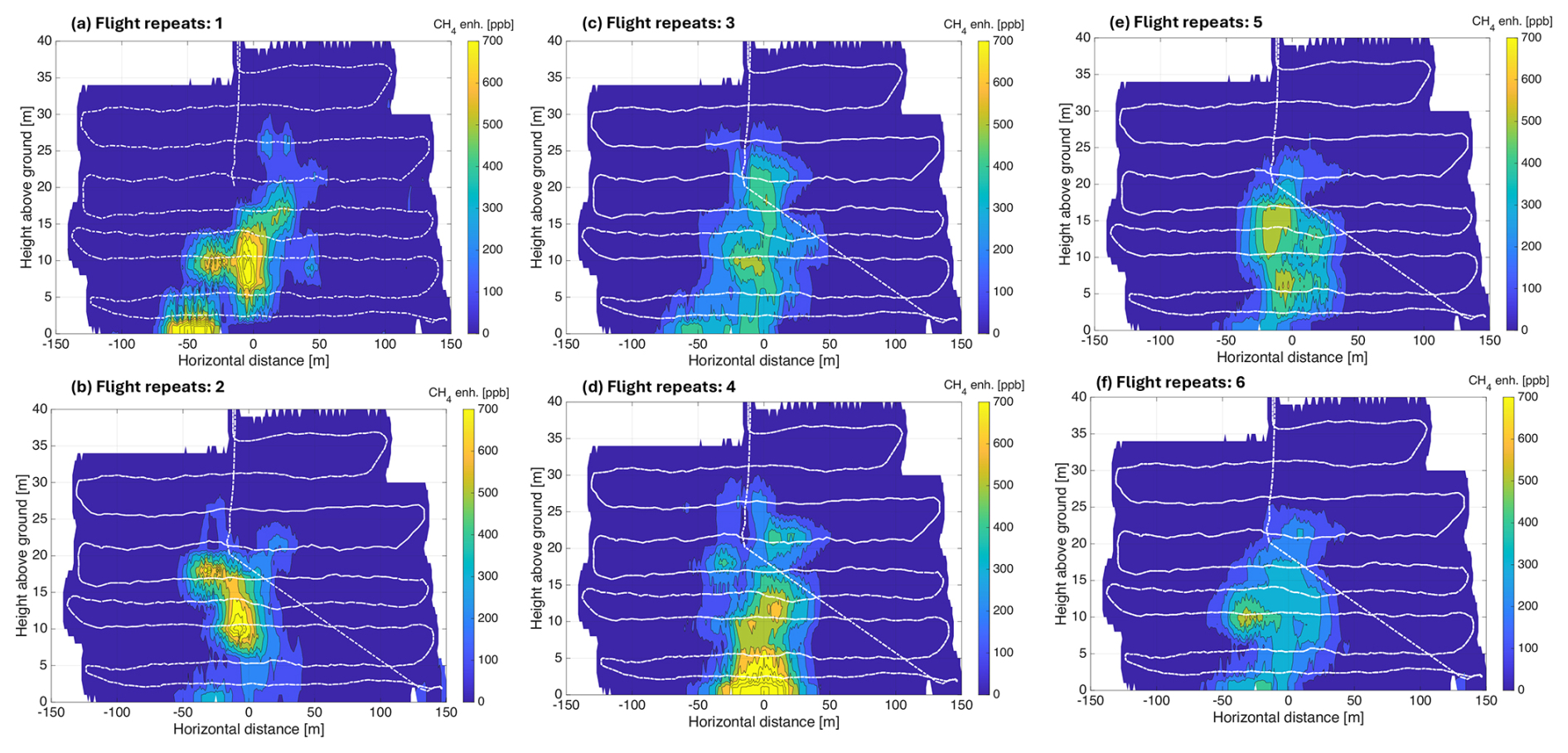
Figure K2 Illustration of sampling of a stochastic plume with an increasing number of flight. Panels (a)–(f) correspond to 1–6 flights, respectively. Increasing number of flights progressively converge toward a Gaussian plume shape. The determined mass emission rates from panel (a) to (f) are: 13.9, 12.3, 10.4, 9.5, 11.1, 10.0 kgCH₄ h⁻¹, respectively.

Appendix L: Uncertainties lower mass emission rates

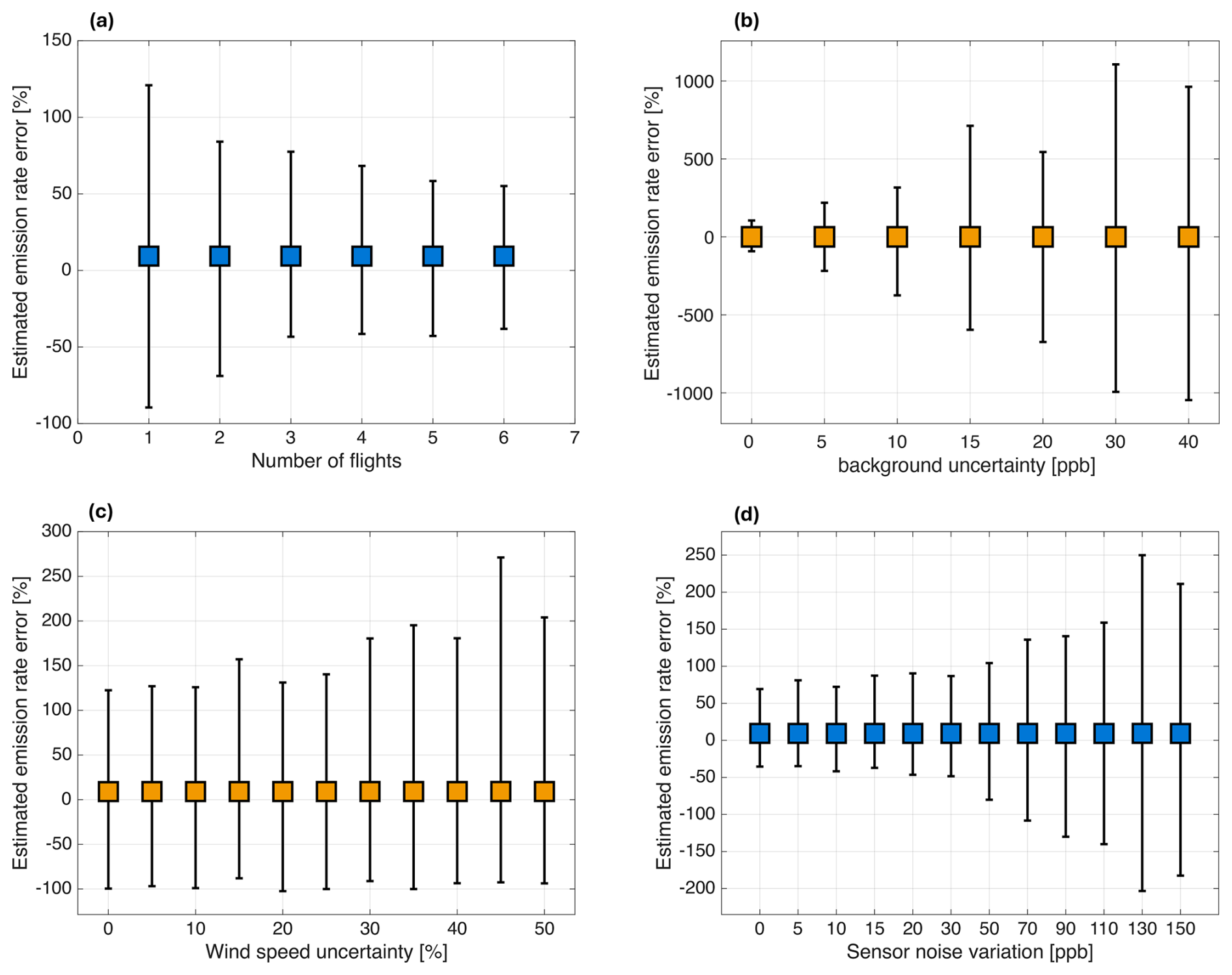
Figure L1 Overview of the individual sources of uncertainty and their respective effect on the estimated error based on a mass emission rate of 1 kgCH₄ h⁻¹.