Design, operation and characterization of a mobile laboratory for hyperlocal atmospheric research

Mobile laboratories equipped with research grade instrumentation make it possible to accurately observe fine scale (< 10 m) concentration gradients driven by local emissions, chemistry and meteorology. The flexibility afforded in measurement location makes mobile monitoring well suited to local pollution source characterization and rapid response to natural and anthropogenic situations. However, constructing a platform capable of these measurements requires simultaneous consideration of many engineering challenges and previous examples are rarely documented in enough open detail for replication. Here, we present the design process and engineering decisions behind the UC Berkeley Mobile Air Pollution Laboratory (CalMAPLab). Built into a Ford Transit 250 van, the laboratory delivers extensive chemical speciation of air pollution in the gaseous and particulate phases. We characterize the performance of the electrical system, climate control and instrumentation suite for mobile measurements with over 500 h of test driving. In addition, we introduce an open-source data acquisition system with live geospatial visualization that facilitates emissions plume mapping throughout a neighborhood. Our detailed description and open design of each critical component reduces the barrier to entry for high-performance mobile monitoring in hyperlocal atmospheric research.

1 Introduction

Understanding the spatial and temporal variability of air pollution is fundamental to assessing population exposure, identifying emission sources, and evaluating the effectiveness of emission-reduction policies. Conventional air-quality monitoring networks provide high-accuracy, continuous long-term records. However, they are spatially sparse. In the US, monitoring stations are separated by 10's of kilometers and are unevenly distributed across certain demographics (Kelly et al., 2024). As a result, fine-scale concentration gradients driven by local emissions, atmospheric chemistry or meteorology remain poorly characterized in many communities. Mobile monitoring has emerged as a powerful complementary technique where the integration of fast response research grade analyzers in a vehicle can produce meter-level spatial resolution while maintaining high data quality (Apte and Manchanda, 2024). Such characteristics facilitate the sampling of real-world air pollution plumes that are both isolated and close to their emission location. With additional benefits related to sampling flexibility, the technique is well suited to the efficient characterisation of local air pollution concerns, and rapid response to natural disasters (e.g. wildfires) or emergency situations (e.g. chemical spills) (Bittner et al., 2024; Liang et al., 2022).

Mobile monitoring can be used to address both scientific and policy-relevant questions. Extensive spatial coverage can detect and quantify natural gas leaks (Defratyka et al., 2021; Vogel et al., 2024; Weller et al., 2019), assess emissions from industrial facilities (Yacovitch et al., 2023), and identify localized hot spots of air pollutants across urban areas (Miller et al., 2020). Intensive applications that involve repeated sampling across different times of day and seasons have enabled estimation of population exposure to criteria pollutants at the city-block scale, revealing fine-scale inequities in air pollution burden (Apte et al., 2017; Marto et al., 2025). Advances in chemically speciated, high-time-resolution measurements have further enabled source fingerprinting and attribution, providing new insights into emissions from traffic, industry, and consumer products, as well as exposure to otherwise unmonitored toxic pollutants (Coggon et al., 2018; Robinson et al., 2024). By mapping concentration gradients downwind of sources, such datasets can also be used to probe atmospheric chemical processing and loss mechanisms through observed spatial decay patterns (Apte et al., 2017; Kozawa et al., 2012). More recently, assimilation of mobile monitoring datasets with other data products like stationary sensor networks and hyperlocal inverse modelling has enabled emissions inventory verification and refinement, bridging the gap between bottom-up inventories and real-world atmospheric behavior (Manchanda et al., 2024).

While mobile monitoring has become more widespread, building and operating a mobile laboratory remains a complex engineering challenge. Powering sensitive, power-hungry scientific instrumentation requires robust electrical systems that can operate reliably in the field, often under variable environmental conditions. Thermal management and vibration isolation are critical to maintaining measurement stability and protecting precision instrumentation. Additional complexities exist in synchronizing multiple 1 Hz data streams with precise GPS timing, often via diverse communication protocols. Each of these challenges have been tackled in the mobile measurement literature, both in dedicated descriptions and in the campaigns built upon them (Bukowiecki et al., 2002; Bush et al., 2015; Popovici et al., 2018; Wagner et al., 2021; Whitehill et al., 2024; Wild et al., 2017; Yacovitch et al., 2023). Comparatively few document all major components, their integration into a complete system and their real-world performance together in one place (Drewnick et al., 2012; Xia et al., 2020). The data acquisition and management software is a particular gap where, if described at all, it typically depends on proprietary tools/software and is not publicly available. Therefore, the reproducibility remains hard and the barrier to entry is high.

The growing demand for mobile monitoring in response to environmental justice and community-scale research highlights the need for open, rigorously engineered, and field-validated mobile laboratory designs. In this context, we present the design and performance evaluation of the UC Berkeley Mobile Air Pollution Laboratory (CalMAPLab). This paper details the design process, engineering decisions, power management, system architecture, data post-processing and an open-source data-acquisition and display framework (termed VanDAQ) necessary for the successful operation of the CalMAPLab. The ability to acquire and visualize data from a diverse range of instrumentation using open-source software (Python, PostgreSQL) rather than reliance on proprietary means (e.g. LabView, IgorPro, DAQFactory) is a key contribution to the atmospheric sciences community. We anticipate this, in combination with detail on all other parts of the system, will reduce the barrier to entry for others interested in hyperlocal atmospheric research.

2 Methodology

Mobile laboratory design faces many challenges and engineering decisions that require careful and parallel consideration for successful construction. The design process should begin with and center on the measurement goals (Sect. 2.1). What variables need to be measured, at what resolution and for how long. With this information, a set of instrumentation can be outlined (Sect. 2.2). Vehicle choice must optimize fit of all the components into limited space, while maximizing driving range flexibility (Sect. 2.3). The amount of energy required to power the mobile laboratory can then be fed into the specification of the electrical system (Sect. 2.4). The location of each component should factor in inlet design and weight distribution (Sect. 2.5/2.6). Components, particularly instrumentation, must be stable in a contained-mobile platform, with sufficient vibration and thermal dampening at the mounting locations, which influences layout and power demands (Sect. 2.2/2.4/2.5). Finally, the components in the data acquisition system must be able to acquire and geolocate information from all instrumentation varieties and consider a range of communication protocols (Sect. 2.7).

2.1 Goal oriented design

The following requirements went into the design of the CalMAPLab:

• Compounds should be measured with Research, Federal Equivalence Method or Federal Reference Method grade instrumentation.

• Sufficient chemical speciation to differentiate sources including key pollutants of concern and provide insights into atmospheric chemistry.

• Ability to collect samples for further offline lab characterization.

• Instrumentation sufficiently fast for high spatial resolution e.g. 1 Hz.

• Instrumentation is stable in a moving platform.

• The electrical system should support 8–10 h of remote stationary or mobile operation and take advantage of widespread charging infrastructure.

• The mobile platform can access all urban roads without considerations beyond normal driving.

• Data from each instrument should be saved in a centralized database that is accessible in real time as time series and geolocated maps for viewing by both the passenger and a central server on the UCB campus.

An overview of the laboratory is given in Fig. 1 with photos in the Supplement (Figs. S1–S3). In the following sections, each major component is discussed in detail.

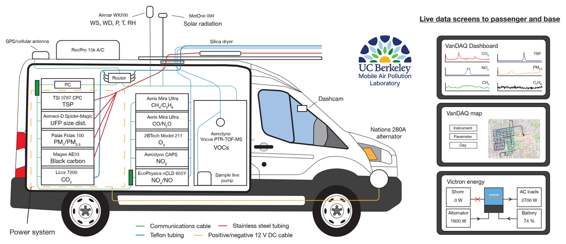
Figure 1 Schematic of the most commonly deployed instrument payload and sampling line layout in the CalMAPLab. Shown are the approximate location of each instrument, sample lines and communication cables, as well as data screens available to the front seat passenger and remote scientists.

2.2 Measurements

The CalMAPLab was designed to provide research grade measurements of major air pollutants, greenhouse gases and other atmospherically relevant tracers at 1 Hz resolution where available. The complete suite of instruments is listed in Table A1 and briefly described below.

2.2.1 VOCs

A Vocus Proton Transfer Reaction Time of Flight Mass Spectrometer (PTR-ToF-MS) was used to quantify hundreds of VOCs that chemically distinguish sources of criteria air pollutants, as well as those that are hazardous air pollutants themselves, or important chemical precursors. Extensive detail and characterisation of the technique exists in the literature (Katz et al., 2025; Krechmer et al., 2018; Pfannerstill et al., 2023; Zhang et al., 2025). The Vocus was set to acquire between mass to charge ($m/z$) range of 18–450 and operated at a $E/N$ ratio of ∼ 120 Td, with the full set of operating conditions and voltages outlined in Table S1 in the Supplement. Average mass resolution during operation was 4800 m Δm⁻¹. VOCs are converted from counts to mixing ratios using a daily calibration factor generated from multi point dilution of a compressed gas standard containing 13 VOCs at ∼ 1 ppm each in zero air (AirGas, Radnor, USA), and an additional zero air background subtraction. Mixing ratios of VOCs not in the standard are estimated via a linear fit of VOC sensitivity versus k_PTR and a default k_PTR of 2.5 × 10⁻⁹ cm³ molec.⁻¹ s⁻¹. Vocus performance mid-drive was verified via short 3 min target calibrations at ∼ 2 ppb (see Sect. 3.1.2), and drift within the CCl${}_{\mathrm{3}}^{+}$ ($m/z$ 116.9) ion.

2.2.2 Other gases

The CalMAPLab measures all gaseous criteria air pollutants except SO₂ (CO, O₃, NO₂) and the top three greenhouse gases by anthropogenic global warming contribution (CO₂, CH₄, N₂O). Most of the instrumentation was chosen based on previously demonstrated stability in mobile applications, and instruments with insufficient published evidence are characterized in Sect. 3.1.2. Two Mira Ultra instruments were used for measurements of CO $/$ N₂O and CH₄ $/$ C₂H₆ with the addition of C₂H₆, which cannot be detected by the Vocus, providing an essential tracer for distinguishing between biogenic and thermogenic CH₄ sources. CO₂ was measured using a LI-7200RS and the accompanying LI-7550 analyzer interface unit. NO₂ was measured with a cavity attenuated phase shift (CAPS) analyzer which ran an internal baseline reading taken every 30 minutes. In addition, NO was measured with a chemiluminescence analyzer, and total NO_x was calculated from the sum of this NO and the CAPS NO₂ measurement. We chose to calculate total NO_x this way, rather than use the NO_x output from the chemiluminescence analyzer due to its use of a molybdenum catalyst which can lead to biases from the conversion of additional NO_y species (Cowan et al., 2024). O₃ is measured with a 2BTech Model 211-G UV absorption analyzer.

Each instrument is calibrated monthly using a multipoint calibration curve. For measurements of CH₄, CO, CO₂, C₂H₆ and N₂O, calibrations are generated from compressed gas standards tied to the WMO GAW scale (Linde, Dublin, Ireland). For NO, NO₂ and O₃, a Model 714 NO₂ $/$ NO $/$ O₃ calibration source (2BTech, Broomfield, USA) is used. Additionally, mid-drive performance for both Mira-Ultra instruments was verified via shorter 3 min target calibrations at the following concentrations: 2.82 ppm CH₄, 13.7 ppb C₂H₆, 251 ppb CO, and 356 ppb N₂O (see Sect. 3.1.2).

2.2.3 Particulate matter

The CalMAPLab aerosol-phase instrumentation package necessitated more deliberate design decisions and compromises than the gas-phase payload. Instrument placement and sampling line design had to take into account flow constraints for each instrument and minimize particle losses as much as possible. We included instrumentation to quantify PM_2.5 as a criteria air pollutant, black carbon (BC) for health and climate impacts, and ultrafine particle (UFP) number counts and size-distributions. A Fidas 100 measures PM₁, PM_2.5, and PM₁₀ simultaneously. Despite being neither a Federal Reference nor Equivalent Method for PM, this instrument was chosen over other options due to it yielding high quality data at fast response times and having inlet requirements that work within the space and size limitations of the vehicle space. Black carbon concentrations were measured with a filter-based AE33 aethalometer as is standard at reference ambient air quality sites across the US. A Model 3789 water-based condensation particle counter (CPC) measures the submicron particle number concentration, which is dominated by ultrafine particles. Finally, a particle mobility spectrometer, made up of a compact radial differential mobility analyzer combined with a Spider-MAGIC water-based CPC and a x-ray neutralizer (Model 3088, TSI, Shoreview, USA), measures aerosol size distribution below approximately 0.5 µm. The Spider-MAGIC was chosen over other sizing options due primarily to its small form factor, high customizability with regards to size range, resolution, and flowrates, and its ability to use multiple neutralization sources without any modifications. The van operates with the X-ray neutralizer so as to negate the challenges and limitations associated with radioactive neutralizers (e.g. Kr-85 or Po-210 which can require licenses and restrict overall platform mobility) though the Spider-MAGIC can operate without any neutralizer if necessary. The standard operating conditions for the Spider-MAGIC are shown in the Supplement (see Table S2) where the instrument is set to measure between ∼ 7–500 nm at 40 bins per decade.

The aerosol instrument package is zeroed and leak-checked using a HEPA filter weekly. The Fidas size distribution is checked with MonoDust 1500 (Palas, Karlsruhe, Germany) annually.

2.2.4 GPS and meteorological parameters

GPS coordinates are captured by a Global Navigation Satellite System evaluation kit and magnetic antenna mounted to the roof. Meteorology is measured with a weather station mounted to the inlet stabilization beams on the roof of the vehicle via a 30 cm pole. This placement removes the station from the slipstream boundary layer of the vehicle itself while also being a completely stable mount, thereby negating the requirement to weld support struts to the vehicle. Many of the commercially available weather stations used in mobile applications can utilize either the NMEA 0183 or NMEA 2000 communications protocols. Despite a limit on the overall data throughput from the weather station, we chose to use the NMEA 0183 protocol due to its ease of conversion to standard serial output and the available open-source development community. Standard operation sets the weather station to report “true” wind speed and direction (corrected from apparent wind using the vehicle's course and speed over ground as calculated via the on-station GPS) as well as ambient temperature and pressure. In addition to ambient meteorology, the CalMAPLab also includes a pyranometer mounted on the roof of the vehicle. The pyranometer and weather station are used to estimate the Pasquill-Gifford atmospheric stability category at any given point in the daytime using the Solar Radiation Delta-T (SRDT) Method (US Environmental Protection Agency, 2000). This is most useful when mapping large-scale plumes (see Sect. 3.2).

2.3 Vehicle size and type

The CalMAPLab is a retrofitted 2023 Ford Transit 250 delivery vehicle with a medium roof height (2.5 m + 0.7 m weather station) and extended 3.8 m (148^′′) wheel base specifications. A number of key considerations went into the purchasing of the vehicle. In general, a larger vehicle is preferred for increased instrumentation space, air circulation and weight capacity. However, for sampling location flexibility and driver availability, our needs dictated that no commercial driver's license would be required. In addition, the vehicle length dimension was limited by the size of our indoor parking space on the UC Berkeley Campus which was deemed necessary for security and 24/7 instrument operation. Multiple heights are available for the Ford Transit. The medium roof option was chosen as a compromise between maximizing space and minimizing the risk of contact with low-hanging cables or tree branches above many smaller roads in California. Although the minimum height is regulated at ∼ 4.6 m (15^′) for communication wires and branches, test driving encountered situations where this was not the case (Public Utilities Commission of the State of California, 2020). Weight was a further consideration and total payload weight was estimated prior to vehicle purchase. The decision to purchase the 250 model (gross vehicle weight rating: 4114 kg, payload capacity: 1635 kg) was made based on model availability and assumptions of a 1490 kg maximum payload (incl. two occupants and a full fuel tank). Finally, electric powered vehicles were considered and tested. Two clear advantages exist over fossil-fuel powered vehicles; there are no exhaust emissions that interfere with sampling and there is a pre-existing battery-electrical system to power instrumentation. While the electric model would have been sufficient for nearby urban sampling, at the time of purchase, the electric model mileage (2023 Ford E-Transit ∼ 187 km less instrumentation power) was deemed insufficient for sampling communities more than 1 h away. The gasoline model chosen has a 25-galllon fuel tank with an average range of 418 km under our operating conditions, which is generally dominated by urban stop/start driving.

2.4 Electrical system

The power demands of all instrumentation in the CalMAPLab, and the associated air conditioning (A/C) was estimated prior to design of the electrical system via laboratory measurements. The total continuous power consumption of the measurement platform is ∼ 3 kW and discussed in detail in Sect. 3.1. The majority of this power is delivered at 120 V AC, with ∼ 200 W at 12 V DC. All equipment, including the A/C, is left running 24/7 to minimize the labor demands and potential instrument drift associated with powering down and restarting instrumentation, as well as ensuring preservation of high vacuum inside the mass spectrometer.

These power requirements can be met by an inverter system tied to a battery bank, engine alternator, external generator or some combination thereof. To facilitate the goals of 8–10 h of stationary and/or mobile operation, a battery-electric system with additional engine alternator charging while driving was chosen. This enabled stationary sampling without the worry of “self-sampling” exhaust emissions, while extending drive time capacity at a lower weight and space cost than a larger battery bank.

A 12 V electrical system with eight 270 Ah LiFePO₄ deep cycle GC3 batteries (Battleborn, Reno, USA) connected to two 2 × 120 Multiplus II 3 kW inverters (Victron Energy, Almere, Netherlands) wired in parallel for up to 6 kW of continuous power draw and 240 A charging capacity (see Fig. 2 for a complete electrical diagram) was installed in the CalMAPLab cargo area. Although the inverter capacity greatly exceeds system power demands, inverter efficiency reduces with temperature (2.5 kW at 25 °C, 2.2 kW at 40 °C, max 93 %), and this buffer room is required when sampling in hot locations. A 12 V secondary, after-market alternator (280XP-2023-UP-PFDI, Nations Starter and Alternator, Cape Girardeau, USA) was installed on the engine with associated regulator (Model WS500, Wakespeed, Reno, USA) and monitoring shunt for ∼ 1.5 kW of continuous power while the engine is running. The options for secondary alternators that fit the 2023 Ford Transit PFDI engine are limited. Since overall system voltage is determined primarily by the second alternator, the electrical system design should be considered in tandem with the vehicle base choice. Higher voltage DC systems may be preferred for smaller diameter wiring. However, this comes at the expense of additional DC-DC converters for powering 12 V equipment.

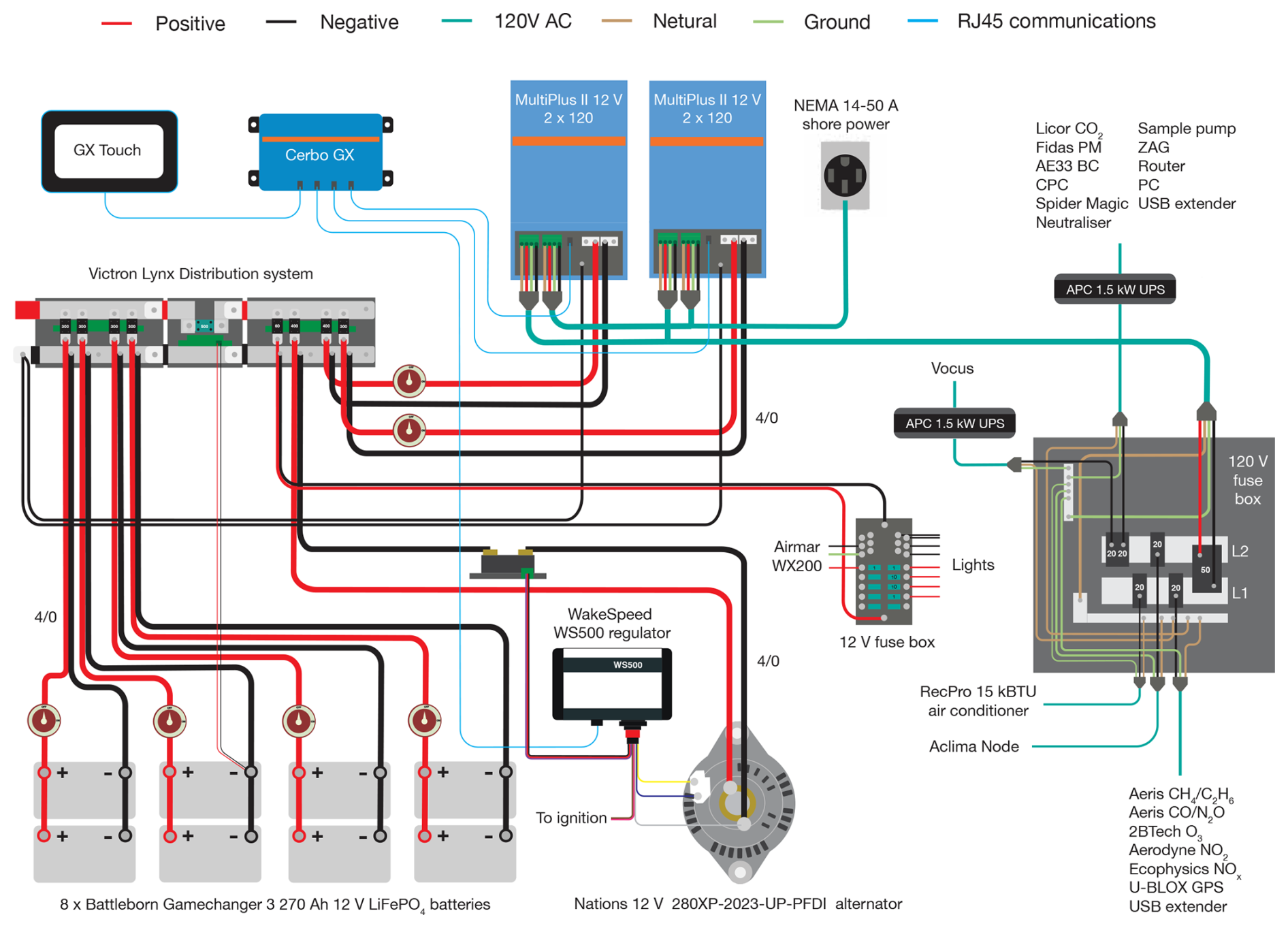
Figure 2 Complete electrical system wiring diagram for the CalMAPLab including the battery bank, busbar distribution and inverter system, as well as fuse box wiring, alternator charging and Victron communications.

The batteries are wired as four separate battery banks, each consisting of two batteries with its own on/off switch. This allows the removal of some battery capacity should space or weight requirements change in the future. The DC loads are combined and fed into the inverters via busbars within Lynx Distributors (Victron Energy, Almere, Netherlands), either side of a Lynx Shunt (Victron Energy, Almere, Netherlands) fitted with a 500 A mega fuse. An additional 12 V DC fuse box (Blue Sea Systems, Menomonee Falls, USA) is wired to the output distributor for power to interior lighting and 12 V instrumentation. All other equipment runs off 120 V AC power generated by the inverters. Four 20 A duplex receptacles are wired to all corners of the van via a 120 V fuse box (Square D, Andover, USA), in addition to a 20 A line for the A/C. It is noted that some efficiency gains could be made by wiring DC instrumentation (e.g. Licor CO₂, CAPS NO₂, 2BTech O₃) directly into the DC supply rather than use supplied adapters. With this payload, the savings are negligible (∼ 10 W) compared to the total power draw. However, should the payload contain a large fraction of DC powered equipment, this is worth consideration. Shore power is provided via a 50 A split phase circuit and NEMA 14–50 plug. This high-capacity infrastructure was chosen to facilitate both overnight battery charging with simultaneous instrument operation, in addition to its common availability at RV parks for field campaign flexibility. The transition from pass through shore power to inverter power is slower on the second hot leg. To prevent power loss to sensitive instrumentation, back-up UPS's (Model 1500, APC Schneider Electric, Rueil-Malmaison, France) are installed on those receptacles. Communication between all electrical components is handled by a Cerbo GX (Victron Energy, Almere, Netherlands) which is connected to the van internal WIFI. All measured parameters are displayed in an online portal for continuous remote monitoring in the front of the vehicle.

2.5 Mechanical and thermal engineering

The platform design incorporated heat management and vibration dampening in order to improve instrument performance. The CalMAPLab was designed to be able to operate in locations with > 30 °C ambient temperatures. Exterior solar heating, especially when stationary without the cooling effect of passing air, will increase the temperature in the van cargo area and cause the instruments to overheat. Additionally, the high thermal load produced by the continuous operation of the inverters and instruments within the cargo space would increase temperatures beyond many instruments' operable ranges when sealed shut without any cooling. To minimize exterior solar heating, the exterior of the van is painted white to increase albedo and the van walls and ceiling are lined with ∼ 5 cm of insulation and a DuraTherm liner (Legend Fleet Solutions, Tillsonburg, Canada). The interior is maintained at ∼ 22 °C with a 15 kBtu A/C (RP-AC3800-P-W-KT, RecPro, Bristol, USA) in combination with two whole-room circulation fans (Vornado, Andover, USA). Thermal regulation performance is evaluated in Sect. 3.1.1.

For vibration dampening, most instrumentation is mounted within two off the shelf 24U 19^′′ server racks each bolted to a shock-rope isolation plate system. The Vocus-PTR-ToF-MS was built into a custom steel rack with similar shock rope isolators for relevant components and mounted to the floor via an L-track locking system. This enables easy removal for major maintenance and payload flexibility. L-track lines were also placed along the floor, walls and ceiling at strategic locations for mounting and securing non-rack-mountable equipment. Particle instruments were placed in the driver's side rack to be in line with the roof inlet hole and minimize the number of bends and resulting particle loss. Both server racks are rotated such that access to the front and rear of each instrument is granted.

The heavy electrical system was placed over the rear wheel base so as to not exceed the front gross axle weight rating (GAWR), and for stability/improved vehicle handling. Other heavy equipment like the Vocus, UPS's and compressed gas cylinders are situated on the opposite side of the vehicle to the battery bank to balance L-R weight distribution. Overall, the weight was measured as 1733 and 2132 kg for the front and rear axles respectively, below GAWR limits of 1873 and 2502 kg.

2.6 Inlet design

The sampling inlet was designed to minimize slip stream and self-sampling, without extending vehicle height to a level that would impact route flexibility. As such, air intakes for the instruments are positioned out the front of the mobile lab via connection to a t-slot metal stability beam secured to two roof racks. Inlet lines then enter through a hole in the roof through bulkhead adapters (Swagelok, Solon, USA) fitted to custom machined plates secured on either side of the aluminum roof. Sample air is then distributed to the different racks and instruments via the flow paths shown in Fig. 3.

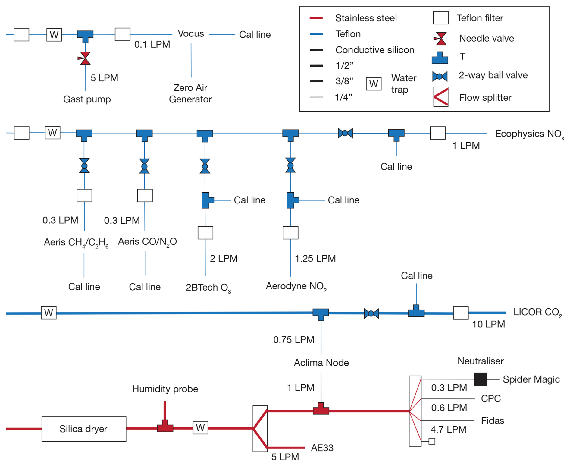
Figure 3 Schematic of the inlet configuration and flows for the three gas phase and singular particle phase sampling lines. Further details on each instrument are provided in Table 1.

There are three gas phase sample lines each made from PTFE to minimize wall losses. The gas rack and Vocus lines are 1/4^′′ OD to minimize lag time. The Licor-7200RS samples from a separate 3/8^′′ OD line through a large HEPA filter (Pall Life Sciences, Port Washington USA) to accommodate the internal pump sensitivity to larger pressure drops. Each instrument has a capped t-piece and 2-way Teflon-valve for connection to a calibration line and isolation from all other instruments. In addition, each instrument has its own filter (DIF-BK60, United Filtration Systems, Sterling Heights, USA) to prevent particle contamination. Flow to the gas rack (∼ 5 slpm) and LI-7200 (∼ 10 slpm) is provided through the internal pumps of the instruments and for a response time of ∼ 1 s (see Table A1 for breakdown by instrument). An additional bypass pump (Model DOA-V751-FB, Gast, Benton Harbor, USA) and needle valve is used on the Vocus inlet plate to increase flow from 100 sccm to 5 slpm for similar response time.

The particle inlet consists of a 1/2^′′ OD stainless steel line fitted with an aerodynamic inlet cone (Brechtel, Hayward, USA) and in-house machined silica bead cartridge dryer. Drying efficiency is continuously monitored with an in-line humidity sensor (HMP 60, Vaisala, Vantaa, Finland). Three flow splitters (Brechtel, Hayward, USA) accurately divide the sample stream and distribute the sample air to each particle phase instrument via short (< 50 cm) sections of conductive tubing. Here, use of non-stainless steel is minimized while maintaining enough flexibility that vehicle motion does not damage the inlet itself. Flow is provided by the instrument's internal pumps for laminar flow (Re = 1400 at 0.43^′′ ID tube diameter, 11 L m⁻¹, 20 °C and 1000 mbar with an entrance length of 0.76 m) up until the flow splitters. Particle loss was estimated for different particle diameters as a percentage loss through the inlet (von der Weiden et al., 2009) with results shown in Fig. S4. When stationary, loss ranges from 6 % for PM_2.5 up to 40 % for the smallest size bins in the sub 10 nm range. As driving speeds increase larger particles are preferentially sampled, increasing sampling efficiency above ∼ 300 nm. This increase can be as high as 40 % for PM_2.5 when driving at speeds of 25 m s⁻¹ (90 km h⁻¹). Under these conditions, an isokinetic inlet is clearly desirable. However, the majority of driving undertaken by the CalMAPLab is carried out at 10 m s⁻¹ (36 km h⁻¹) where the effect is minimal. As such, the additional expense of such an inlet could not be justified. All four sample inlets have a water trap installed to prevent instrument contamination in heavy rain.

2.7 Data acquisition system and visualisation

The design requirements for the CalMAPLab data acquisition system were to (a) acquire and synchronize measurements from a variety of instrumentation at the finest time resolution supported by each instrument, (b) accurately geolocate each timestamp with GPS data, (c) efficiently store and back up all data, (d) provide real time visualisation of select data both as time series and spatially on a map, both locally and remotely, (e) facilitate valve actuation for calibrations and (f) be flexible enough to support changes in instrument payload without code changes. To accomplish that, data-streams from each instrument are collected with a custom data acquisition system referred to as VanDAQ, the architecture of which is shown in Fig. 4a. The hardware running VanDAQ consists of 2 separate Linux-operated computer systems: a low-power mobile server (Vault Pro VP6670-6, Protectli, Vista, USA) in the vehicle and a stationary server located on the UCB Campus. RS232 serial, USB, and Ethernet data connections link each instrument to the mobile server and a number of Python software processes facilitate data transfer into a local PostgreSQL database. The data is also packaged as one-minute files and transmitted over a cellular-WIFI data link via a 5G router (MOFI6500-5GXeLTE, MoFi Network, Toronto, Canada) to the central server which ingests data to the central database. While this feature was not used during testing, the architecture supports multiple mobile servers running the same software, all reporting data to the central server with a unique platform identifier. All processes in VanDAQ are written in open-source software (Python, PostgreSQL) and maintained on a publicly available repository (https://github.com/CalMAPLab, last access: 22 June 2026).

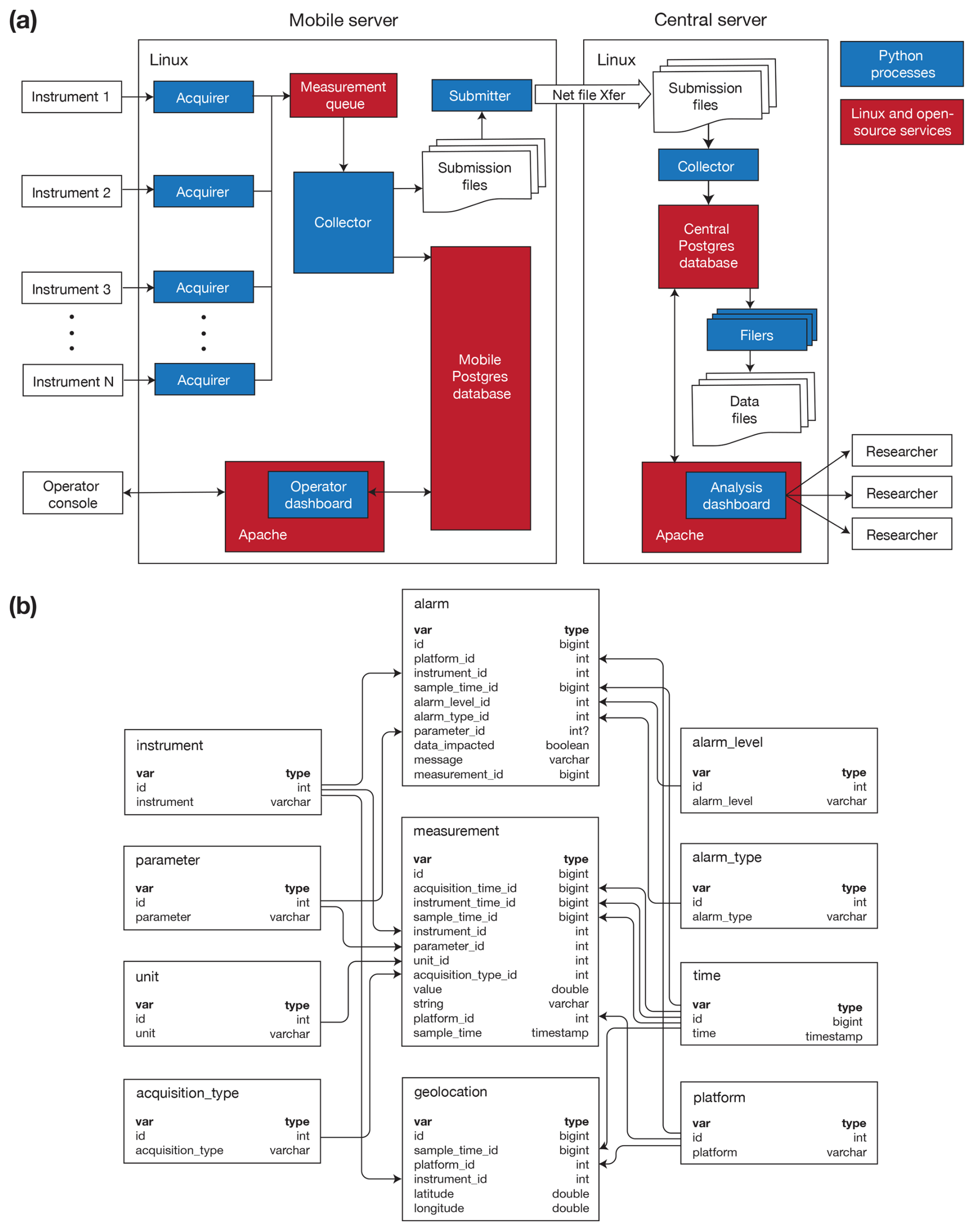
Figure 4 VanDAQ architecture diagrams for (a) the data pipeline from generation in the instruments to processing via the mobile and central servers and (b) the database schema for all measurements, alarms and supporting meta data.

Each instrument in the mobile platform is serviced by an acquirer process. The acquirer is a Python script that is configurable via a text file to acquire data based on the data link style, protocol and format unique to each instrument. Therefore, there is only one acquirer code body that is launched into multiple processes configured to each instrument. The acquirer is the only software component in the system that understands the unique communication needs of the instruments, converting the data into a common-currency exchange format consisting of a Python dictionary for each individual data value with metadata describing the platform, instrument, type, parameter, and unit of the data item. Configuration file format, including examples and how to set up a new instrument, are detailed in the GitHub repository documentation. The system is SNTP-disciplined and synchronized by system-timesyncd with time alignment across instruments established from deployment of acquirers on a single acquisition computer. Each acquirer process timestamps its records using the shared host wall clock with a 1 s resolution. Possible skew between acquirers is bounded by serial latency, process scheduling and queue handoff. We measure a maximum timestamp skew between pairwise observations of 1 s from acquirers stamping adjacent seconds 0.3 % to 0.5 % of the time. The unified and packaged measurement data are loaded by the various acquirer processes into a single POSIX interprocess communications (IPC) queue (max messages = 50, max data per message = 8 kb) for further processing downstream. Overall, this feature of the VanDAQ architecture facilitates the incorporation of various diverse instruments and changing payloads without change to the rest of the system downstream of the acquirer.

In the van the measurement queue is unloaded by the Collector process which (1) loads the data items into the mobile server's PostgreSQL database via batched row INSERT and (2) packages the measurement dictionaries into one-minute submission data files for transmission to the central server. As the Acquirer is the only process that knows how instruments communicate, the collector is the only component which deals with the intricacies of loading the PostgreSQL database. Ingestion performance was quantified from production collector logs with an average sustained throughput of ∼ 1300 rows s⁻¹ compared to an average arrival rate of ∼ 160 rows s⁻¹ from roughly 160 1 Hz instrument-parameter pairs (including some engineering data). This indicated significant operational headroom for continuous acquisition with the current instrument payload. Durability of the system is primarily provided by the PostgreSQL database. Following power loss, only data within the IPC and therefore uncommitted to the database is lost.

The computer system runs an operator dashboard website which is hosted on an Apache HTTP server and available via the van's internal WIFI network. The dashboard displays graphical time series of measurement parameters produced by all instruments, alarm states, and a real-time street map with data tracks and wind rose plotting (see Figs. S5–S9). Shape files can be uploaded to the server to highlight areas of interest on the map during a drive. In addition, a control panel is set up to send various serial commands for valve triggering and calibrations.

The submission files are transferred via cellular or WIFI link to the central server by the van's Submitter process. Submission of data files to the central server is asynchronous and can deliver data for ingestion into the central database in near-real-time (1+ min latency) or, depending on the state of the mobile network link, will store data files and submit when possible. Another collector process on the central server ingests data from the submission files and inserts measurements into the central database, whose schema is a duplicate of the mobile database(s). The central server also hosts an analysis dashboard website allowing researchers to browse historical data, monitor the current state of the van, and observe mapped data collection in near-real-time remotely.

The Postgres database schema (see Fig. 4b) on both the mobile and stationary servers follows a star data model, with two central fact tables for instrument measurement values and alarms, and dimension tables for alarm level and type, mobile platform ID, instrument, acquisition type (e.g. environmental measurement, instrument engineering value, or geolocation), parameter name, measurement unit, timestamp, and geolocation. The dimension table contents are dynamically built from incoming measurement metadata, so that new measurement types can be accommodated without changes to database structure or requirements for direct dimension table maintenance. The geolocation dimension table is assembled from incoming GPS instrument data identified by the “gps” acquisition type (which otherwise are treated the same as all instrument measurements), with columns for platform, instrument (GPS unit), and timestamp IDs. Multiple GPS receivers can be accommodated on the mobile platform(s), with the most accurate or relevant geolocation stream selectable for the given output. Instrument data queried for map display or geolocated raw data files are joined to the geolocation table by sample time, filtered by platform and selected GPS receiver.

Acquired data are visualized via a Python web application built on the Dash framework (Plotly Technologies Inc.) (Carson Sievert, 2020). The application queries data through a SQLAlchemy interface (Bayer, 2012), and provides last-5 min time series plots of data acquired by all instruments for diagnostic purposes, a dynamic table of alarms, a live map display, and a page of instrument controls. The app is hosted on both mobile and stationary servers by the Apache2 web server (Apache Software Foundation).

2.8 Post processing correction pipeline

Post-drive, raw files are generated from the database based on pre-determined criteria (default is all time stamps where GPS is not equal to NA). These files are then post corrected with a custom adaptable workflow. First, data from each instrument is lag corrected for sample and instrument response delays such that data points line up with the correct geolocation. This is done monthly by burning a lighter at the inlet and documenting the time each instrument's concentrations change and is validated by calculating covariances between different species across different lags (see Fig. S10). Data from instruments which sample at frequencies above 1 Hz is also averaged to 1 Hz.

Next, the raw GPS coordinates are cleaned to correct positional inaccuracies and gap-fill missing timesteps. A Kalman filter is applied to smooth the coordinates before they are linearly interpolation to 1 Hz. This step is necessary since the u-blox GPS output is slightly less than 1 Hz (average 0.8 Hz) and NA removal would lead to loss of valid chemical measurements. Coordinates are then snapped to road geometries to standardize locations, with preferential matching to road segments with directions within 60° of the GPS bearing. These road linestrings are created from the OpenStreetMap (OSM) database by grouping continuous roads of the same name and direction, then splitting these grouped geometries into short road segments which are identified by centerpoint coordinates (OpenStreetMap contributors, 2017). Each 1 Hz sample is matched to these smaller road segments, typically 30 m lengths, and H3 indices for spatial aggregation. Individual drive pass statistics are generated based on a time threshold exceedance (default 30 s) between visits to a 30 m segment ID. Aggregation at these coarser temporal and spatial scales is then made depending on the visualisation required. Each of these transformational steps is shown in Fig. 5.

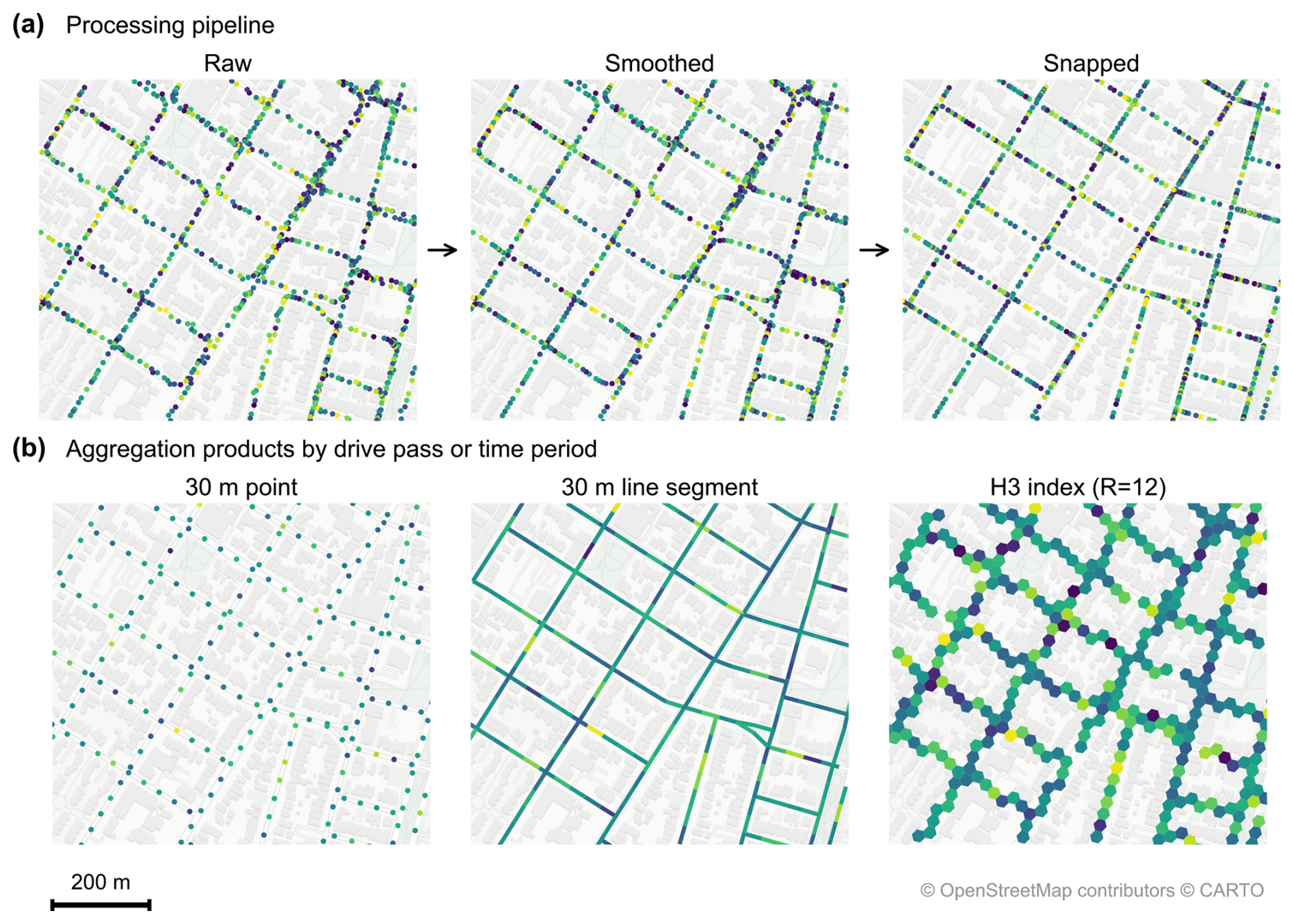
Figure 5 (a) GPS processing pipeline for missing data and positional correction and (b) three visualisation methods for aggregating multiple passes of a given road segment. The color in the raw dataset is a randomly generated integer to help distinguish data points. Map tile data courtesy of OpenStreetMap contributors, distributed under the Open Data Commons Open Database License v1.0.

Following GPS processing, calibrations are linearly interpolated and then applied. Finally, data is flagged based on engineering parameters to remove periods of suspect data and calibration times.

3 Initial applications

The CalMAPLab performance was evaluated over the course of more than 500 h of driving in the San Francisco Bay Area throughout 2025. Overall, the platform demonstrated excellent reliability and high data quality. Here we examine the performance of the facility over this test period and detail its application in plume tracking over a mixed residential and industrial neighborhood.

3.1 Performance overview

3.1.1 Electrical system and thermal regulation

Initial performance here we define as the reliability and robustness of the electrical system and the climate control of the van cargo interior. We focus on these two areas as they were priorities in the system design to optimize instrument performance. In the original design of the platform, the total power draw of the intended payload was estimated as 1.4 kW (A/C fan only) and 2.7 kW (A/C cooling). An additional 15 % overhead was added for anticipated efficiency losses in the system. This turned out to be a good estimate for those conditions. Average power drawn by the instrumentation from the inverters during the testing drives was 2.3 kW (range 1.6–2.8 kW), with a peak load of 3.2 kW. However, average power drawn from the batteries was higher at 2.7 kW (range 1.8–3.2 kW) and a peak draw of 3.8 kW, reflecting an average efficiency loss from batteries to inverter output of 15 %. The variability between sampling days was largely explained by ambient temperature and its influence on A/C running time.

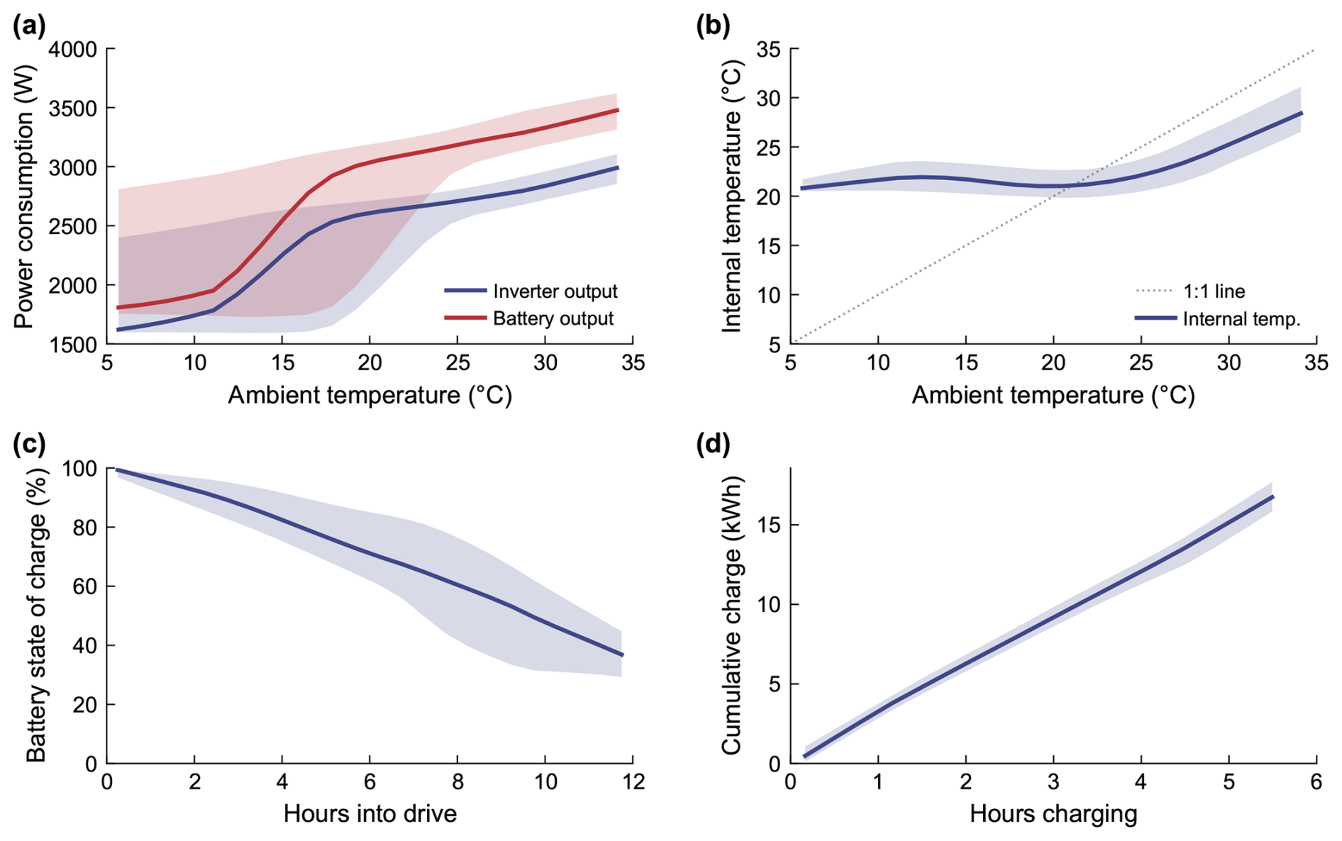
Figure 6 Data from the Victron electrical system showcasing (a) the power throughput of the batteries and inverters at different ambient temperatures, (b) the response of cargo area internal temperature to ambient temperature during operation, (c) the battery state of charge throughout each drive and (d) the charging rate when connected to shore power. Plotted are the locally weighted scatterplot smoothed functions of the 5 min electrical data with 10th and 90th percentile confidence intervals.

This is demonstrated in Fig. 6a between 5 and 25 °C ambient temperature where the high variation reflects a cluster of measurements at lower power consumption during which the A/C cooling cycle is off. Above this temperature, the A/C is in continuous cooling operation and power draw gradually increases. This is likely a consequence of an increase in cargo area temperature (Fig. 6b) causing higher power draw from instrument pumps to maintain the same performance, and/or a further reduction in the efficiency of the electrical system. Although the A/C is not sufficient at maintaining the cargo area temperature above 26 °C ambient, it remains ∼ 7 °C lower and no noticeable degradation in instrument performance was observed during sampling of up to 35 °C (see Sect. 3.1.2). Should extended periods of sampling at these temperatures or higher be required, additional A/C tonnage would likely be necessary. However, within our typical sampling domain, these elevated temperature periods typically only last for a few hours in the early afternoon, and the cargo area temperature recovers once ambient temperature begins to drop. The mobile laboratory was not tested in sub-zero conditions. However, the RecPro HVAC system can heat the interior via a heat pump if required. In addition, temperature sensitive components in the Vocus reagent ion delivery system like the water bottle and reagent line are heated with heat tape to prevent condensation and irregular delivery flows.

Some atmospheric measurements are sensitive to the density and therefore temperature of the sample gas. To assess thermal transients along the sampling path, we compare roof ambient temperature with sample gas temperatures reported at the cell inlet of the Licor 7200. On average, the median daily temperature range on the roof was 7.7 °C (min = 0.3 °C, max = 22.4 °C) whereas median daily ranges at the Licor was 2.1 °C (min = 0.1 °C, max = 12.4 °C, see Fig. S11 for more detail). These results indicate substantial thermal buffering of sample air relative to roof ambient, consistent with heating and residence time in the climate-controlled cabin rather than directly tracking outdoor temperature. For uncorrected density-sensitive measurements, biases are estimated at ∼ 1% rising to ∼ 3% on the days with greatest temperature variability. Within our instrument payload, these are largely accounted for through measured cell temperature and subsequent internal corrections. In addition, no condensation issues were encountered where sample dew point was at least 5 °C below the van internal temperature 100 % of the time. However, we do note that should sampling take place in more humid environments, heating the sample line is an important consideration.

The power system's storage capacity was sufficient for our needs throughout the test period duration. The battery state of charge (SOC) distribution for each drive is shown in Fig. 6c where the minimum end SOC was 25 % corresponding to a maximum drive length of 12 hours and hot ambient conditions. As noted previously, the spread reflects variation in power consumption in relation to changes in ambient temperature. While these Battleborn batteries are designed for 100 % discharge, this is not the case for all manufacturers, or battery chemistry types. On average, the second engine alternator provided 1.6 kW of charging during each drive and was an effective alternative to additional heavy battery capacity. Overall charging rate was very consistent (see Fig. 6d) at ∼ 3.2 kW corresponding to an 8 h full charge time. To operate the instrumentation and charge the batteries, shore power draw during charging reached a maximum of 6.8 kW highlighting the need for NEMA 14–50 infrastructure at this charging rate.

3.1.2 Measurement stability

Much of the instrument payload was chosen based on past reliability in mobile applications (Apte et al., 2017; Harlass et al., 2024; Ma, 2021; Padilla et al., 2022; Shah et al., 2023) and long-term stability was observed in the calibration factors across the testing time period (see Fig. S12). The 2BTech Model 211-G exhibited some motion dependence on speed bumps or large potholes that resulted in unrealistic spikes in the data (see Fig. S13). This was despite the installation of rope-shock mounts and additional foam support system. However, since we are most interested in O₃ gradients over larger spatial scales, with spike removal and averaging this was not considered a major issue.

Both Aeris Mira Ultra gas analyzers are less well characterized in the literature, so additional target calibrations were performed mid-drive to monitor instrument drift due to changing environmental conditions. All species exhibited low drift and measurement bias during individual drives (see Fig. 7a/b for examples). Overall bias in the measurements was CH₄: 18.9 ppb, C₂H₆: −0.1 ppb, CO: −2.0 ppb, N₂O: −0.8 ppb, well within the 10 % calibration standard uncertainty. The target calibration measurements are largely normally distributed with a 1 Hz precision given as the standard deviation in the measurements for CH₄: 1.6 ppb, C₂H₆: 0.2 ppb, CO: 0.6 ppb, N₂O: 1.1 ppb.

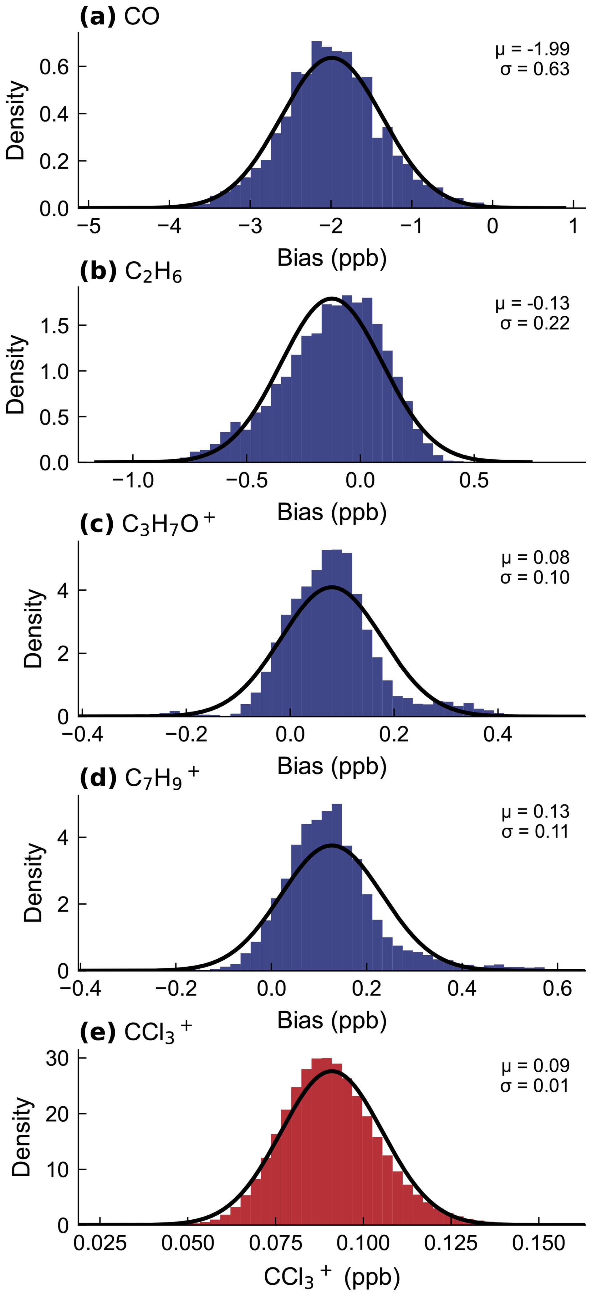
Figure 7 In-drive performance characterisation of the select species from the two Aeris Mira Ultras (a–b) and Vocus PTR-ToF-MS (c–d) via target calibrations. Shown are the distributions of the measured concentration minus calibration standard concentration, with details on the mean (μ) and standard deviation (σ) for 1 Hz measurements. Also shown is the distribution of complete drive CCl${}_{\mathrm{3}}^{+}$ concentrations, excluding some periods of local emission (e). Note, the concentration is only determined via the relationship of k_PTR and sensitivity, rather than direct calibration with a standard. Fitted normal distributions are plotted as black lines.

Similar target calibrations were conducted on the Vocus PTR-ToF-MS for each of the compounds in the calibration mix (see examples in Fig. 7c/d, and statistics in Table S3). Measured bias was low for all compounds and within calibration uncertainty. However, precision did vary considerably between species. Mass C₂H₇O⁺, which is used for quantification of ethanol, was notably worse due to the much lower sensitivity of that compound in the instrument. We also observe a small but increasing temperature dependence by $m/z$ for the higher molecular weight hydrocarbons that results in a reduction in precision. Comparison with the CCl${}_{\mathrm{3}}^{+}$ concentration distributions during each drive (see Fig. 7e) indicates this issue is related to the calibration set up rather than the instrument sensitivity. CCl${}_{\mathrm{3}}^{+}$ is the major ion of trichlorofluoromethane and carbon tetrachloride, two stable, long-lived ozone-depleting compounds now banned under the Montreal Protocol. As such, concentrations are extremely stable, and the ion can essentially be used as an internal standard (Notø and Holzinger, 2024). No drift was observed in the post calibration CCl${}_{\mathrm{3}}^{+}$ measurements implying that the calibration schedule well captures any change in instrument performance. Therefore, the target temperature dependence is attributed to an increase in off gassing in the high-concentration conditioned calibration line at higher temperatures. This would impact higher molecular weight compounds more and would add a similar bias to each step of the multipoint calibrations, thereby not impacting slope calculation.

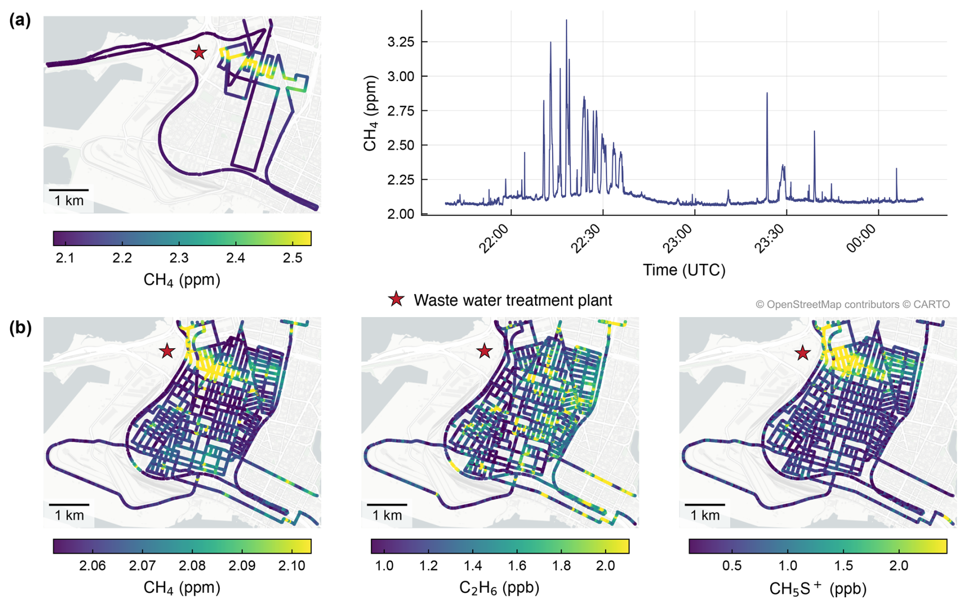
Figure 8 Examples of urban pollution mapping in the West Oakland neighborhood, CA, facilitated by live spatial visualisation within VanDAQ. (a) Efficient on-the-fly turn by turn routing enabled through coloring of GPS data points compared to time series plotting and (b) full neighborhood drive coverage enabled through live tracking of previously sampled roads. All color scales are capped at the 5th and 95th percentiles as are in the software for clarity. Map tile data courtesy of OpenStreetMap contributors, distributed under the Open Data Commons Open Database License v1.0.

Although stable, some instrumentation is not sufficiently precise to produce high quality data at 1 Hz frequency. An example here is the EcoPhysics NO₂ measurement which the instrument calculates by subtracting NO from the total NO_x. The additional noise introduced by this step and the conversion catalyst is visible in the raw 1 Hz data when compared to the CAPS NO₂ measurement (see Fig. S14). However, by aggregating to longer time periods a much better agreement is observed. In these situations, repeated passes and aggregation to larger spatial scales can mitigate most of this uncertainty.

3.2 Urban plume mapping with VanDAQ

Live visualization of geolocated data was essential for VanDAQ's data acquisition system, serving two primary functions: tracking drive progress when sampling all roads in a neighborhood, and enabling on-the-fly routing decisions when tracing emission plumes based on spatial concentration gradients. Figure 8 demonstrates both capabilities. Panel (a) shows how real-time visualization of spatial gradients enabled efficient mapping of a large CH₄ emissions plume through West Oakland, CA. While the time series data alone does indicate elevated concentrations, the visual cues within the map provide intuitive tracing of the impacted area and clear guidance on where to sample next. Panel (b) highlights the importance of this visualization for neighborhood-wide sampling, where the sheer number of roads makes routing from memory impractical. Here, we see that same emissions plume fully mapped out with a clear impacted area in the north. This particular example can be attributed to emissions from a wastewater treatment plant (WWTP) to the west through the chemical speciation provided by CalMAPLab, whereby the lack of C₂H₆ in the CH₄ plume rules out natural gas, but the presence of odorous sulfur compounds like methanethiol (CH₄S) that are commonly associated with WWTP processes is compelling evidence for that facility (Li et al., 2021). Without real-time mapping, such semi-transient emission events could easily be missed or misattributed, particularly in areas without prior knowledge of sources. VanDAQ's live visualization allows users to identify unexpected features in any incoming data stream and adapt drive plans accordingly.

4 Conclusions

Mobile laboratories are a valuable resource for characterizing air pollution at the hyperlocal scale, yet detailed documentation of their design and real-world performance remains limited. Here, we have presented a comprehensive description of the UC Berkeley Mobile Air Pollution Laboratory (CalMAPLab), a platform which produces high spatial and chemical resolution measurements of gaseous and particulate air pollutants. With 15 reference or research grade analyzers built into a compact design, we are able to quantify most criteria air pollutants as well as a wide range of other air toxics and atmospheric tracers while maintaining a sampling flexibility not afforded by larger vehicles.

Performance evaluation over 500 hours of driving demonstrated reliable operation across a range of ambient conditions. The battery-electric system with secondary engine alternator sustained average power consumption of 1.8–3.2 kW for up to 12 h during testing, with 15 % efficiency loss between battery storage and inverter output underscoring the importance of building overhead into electrical system specifications. Thermal management emerged as a critical constraint with the air conditioning system maintaining cargo temperatures up to 26 °C ambient, although no differences in instrument performance were observed up to 35 °C ambient. We acknowledge limitations in the particle sampling inlet with size dependent losses through the system, particularly at high vehicle speed. Although with a higher budget, we note that fully isokinetic solutions exist.

The open-source VanDAQ data acquisition system addresses a gap in mobile monitoring infrastructure by providing a flexible, instrument-agnostic framework for synchronized data collection, GPS integration and real-time visualization. The real-time map display allows for adaptive sampling, as demonstrated through emissions plume tracing in West Oakland where live visualization enabled spontaneous routing decisions to characterise plume spatial extents.

In providing detailed documentation of engineering decisions, system architecture and quantitative performance characterization, we aim to lower barriers to mobile laboratory construction and hyperlocal air quality research.

Appendix A

Table A1 List of parameters measured with the CalMAPLab with associated instrumentation and technical details.

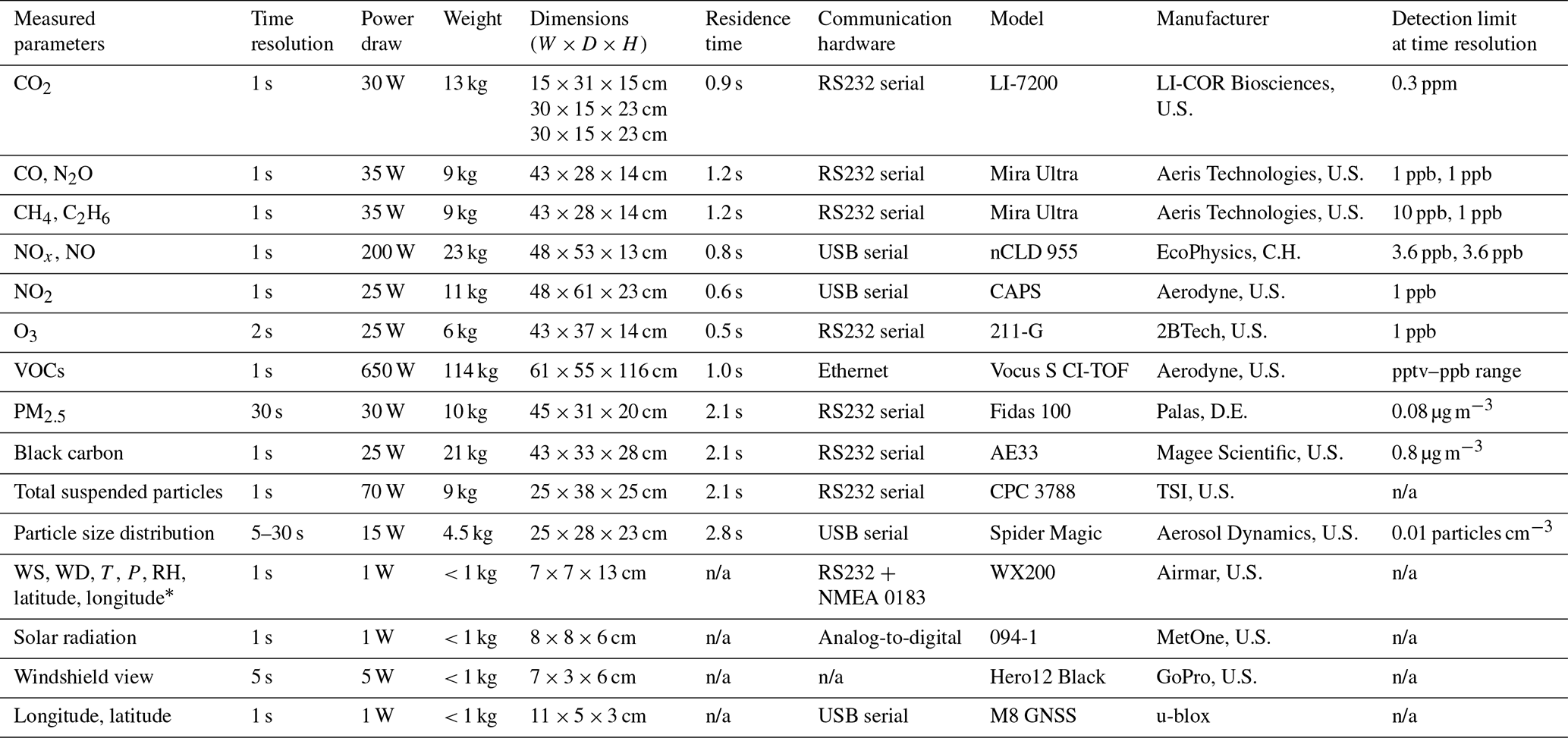
^* WS = Wind Speed, WD = Wind Direction, T = Temperature, P = Pressure, RH = Relative Humidity. n/a: not applicable