Machine learning-based emission rate estimates of global methane super-emissions

Methane, the second most important anthropogenic greenhouse gas, has a global warming potential more than 80 times that of carbon dioxide over a 20-year period. Given its decadal atmospheric lifetime, reducing anthropogenic methane emissions is critical for limiting near-term warming. The TROPOspheric Monitoring Instrument (TROPOMI) provides daily global methane satellite observations, enabling rapid detection of super-emitters. Here, we develop ML-SPERE, a machine-learning framework based on a convolutional neural network trained on simulated TROPOMI methane observations and meteorological data to estimate emission rates for super-emitters. ML-SPERE outperforms the Integrated Mass Enhancement (IME) method on simulated plumes that incorporate real TROPOMI backgrounds and missing spatial data, reducing the median absolute percentage error from 42.4 % to 24.3 % for well-observed methane plumes. At low wind speeds, IME estimates exhibit a negative bias and ML-SPERE estimates do not. Applied to TROPOMI observations of a 200-d well blowout in Kazakhstan, ML-SPERE typically shows agreement with TROPOMI inverse modeling results and TROPOMI IME estimates. Compared to TROPOMI IME estimates, ML-SPERE estimates show improved agreement with IME estimates derived from high-resolution point-source imagers. Global spatial patterns of methane emissions inferred from ML-SPERE and the IME method for all super-emitters found by TROPOMI in 2021 are broadly consistent, with notable regional differences in northern Russia (where transient pipeline emissions may not be well characterized by either method), the Congo Basin (where area source emissions may not be well characterized by either method), and southeastern Australia (where IME estimates are potentially negatively biased owing to predominantly low wind speeds). Mean estimated emission rates for this dataset aggregated by estimated source sector remain similar between both methods. Overall, improved performance on simulated plumes and consistency with independent estimates for real-world observations demonstrate the utility of ML-SPERE for quantifying TROPOMI methane super-emitters.

1 Introduction

Methane (CH₄) is a powerful greenhouse gas, with a global warming potential more than 80 times greater than that of carbon dioxide (CO₂) over a 20-year time horizon (Intergovernmental Panel On Climate Change (IPCC), 2023). Due to its stronger radiative forcing and far shorter atmospheric lifetime compared to carbon dioxide, reducing anthropogenic methane emissions offers one of the most effective strategies for mitigating near-term climate change (Ocko et al., 2021). Super-emitters contribute disproportionately to total anthropogenic emissions, are frequently associated with correctable abnormal operating conditions, and can be highly transient (Zavala-Araiza et al., 2017). Satellite observations have thus proven instrumental in detecting and abating methane emissions from super-emitters (Irakulis-Loitxate et al., 2022; United Nations Environment Programme, 2025). The TROPOspheric Monitoring Instrument (TROPOMI), launched in 2017 aboard the Sentinel-5P satellite, provides daily global observations of atmospheric methane concentrations (Veefkind et al., 2012; Hu et al., 2018; Lorente et al., 2021, 2023). With a spatial resolution down to 5.5 km×7 km at nadir, TROPOMI can be used to detect localized methane plumes associated with super-emitting point sources (Pandey et al., 2019; Lauvaux et al., 2022). These observations can be used to provide emission rate estimates and guide follow-up observations with high-resolution (∼25 m) satellite instruments (Schuit et al., 2023a), all of which can provide vital insight into global anthropogenic methane emissions on a near-real-time basis (Copernicus Atmospheric Monitoring Service, 2025). However, commonly used mass-balance and inverse modeling approaches for estimating emission rates for super-emitting methane plumes found in TROPOMI observations involve trade-offs between accuracy and computational cost, motivating the development of alternative methods that can efficiently quantify large numbers of plumes. We have thus developed a machine learning (ML)-based methodology for estimating super-emitter methane emission rates from TROPOMI observations.

ML techniques have been applied to detect (but not to estimate emission rates for) methane plumes in TROPOMI data on a daily basis (Schuit et al., 2023a). Such automated approaches are valuable given the impracticality of manually screening large datasets. Schuit et al. (2023a) trained a Convolutional Neural Network (CNN) to classify TROPOMI methane scenes as either likely or unlikely to contain a super-emitting plume, and employed a Support Vector Classifier (SVC) to reduce false positives prior to human verification. They also used the CNN to generate plume masks by combining the network's class activation map with a scene-specific methane threshold to delineate the plume. Applying this framework to all TROPOMI orbits in 2021 produced a catalog of nearly 3000 detections. Using bottom-up inventories, these detections were linked to the most likely underlying source sectors including urban areas, landfills, gas infrastructure, oil infrastructure, and coal mines.

Schuit et al. (2023a) estimated methane emission rates for their detected TROPOMI plumes via the Integrated Mass Enhancement (IME) method, first developed for use with aircraft and high-resolution satellite observations of atmospheric methane concentrations (Frankenberg et al., 2016; Varon et al., 2018). This mass-balance-based technique estimates emission rates by integrating the excess methane mass within a plume relative to the local background concentration and dividing it by the plume's residence time, which is typically inferred from the length of the plume and meteorological wind data. The accuracy of this method depends on several factors. Potential sources of uncertainty include the conversion of satellite-retrieved methane columns into plume enhancements and the subsequent delineation of plume pixels from background pixels (Varon et al., 2018; Schuit et al., 2023a). However, the dominant source of error arises from uncertainties in the wind field used to estimate the residence time. Wind datasets often show discrepancies of up to 50 % when compared to in-situ wind measurements at ground stations or airfields (Varon et al., 2018). Moreover, the IME method requires the estimation of an effective wind speed that accounts not only for advection, but also for plume dispersion, diffusion processes, and plume rise. These effective wind speed calibrations are typically estimated using relationships with 10 m wind speeds, rely on simulated plumes, are instrument-specific, and show significant scatter (Varon et al., 2018; Schuit et al., 2023a). The IME method used in Schuit et al. (2023a) is an ensemble approach, and uncertainties are estimated by varying plume masking thresholds, background concentration estimates, and using three separate wind datasets to compute emission rates. Other mass-balance-based approaches like the cross-sectional flux (CSF) method (Varon et al., 2019) and variants of the IME method (Hakkarainen et al., 2025) can also be applied to estimate methane emission rates from TROPOMI plumes and have similar uncertainties. Atmospheric inversions (e.g. Maasakkers et al., 2022a; Lauvaux et al., 2022) provide another avenue for estimating plume-level emission rates using atmospheric transport simulations. Compared with mass-balance approaches, Bayesian inversion methods provide emission-rate estimates that are more explicitly constrained by atmospheric transport physics and are therefore generally better suited to complex meteorological conditions and source configurations (e.g. overlapping sources), albeit at substantially greater computational cost and under the assumption that atmospheric transport can be modeled accurately.

In response to the known limitations of mass-balance-based methods and the computational burden of atmospheric inversions, recent research has explored ML-based alternatives for estimating methane emission rates from point sources (Jacob et al., 2022). CNNs, a class of machine learning models well-suited for image-based tasks, have demonstrated strong performance in both classification and regression applications (LeCun et al., 1989, 2010; Krizhevsky et al., 2012; Toshev and Szegedy, 2014). In the context of methane remote sensing, CNNs have recently been applied to estimate point source emission rates directly from plume imagery (in addition to detection applications), offering the potential to reduce or eliminate dependence on meteorological datasets (Jongaramrungruang et al., 2022; Plewa et al., 2025). Like other machine learning methods, CNNs are trained using input–output pairs, which in this case are methane plume images derived from satellite observations and corresponding known emission rates. Because real satellite observations never come with precise known emissions (except for controlled release experiments), training typically relies on simulated plumes (Jongaramrungruang et al., 2022; Joyce et al., 2023; Radman et al., 2023; Bruno et al., 2024; Plewa et al., 2025), where the emission rate is known for each generated image. CNN-based methods have shown promising results when applied to high-resolution satellite or airborne observations (Joyce et al., 2023). MethaNet (Jongaramrungruang et al., 2022) was able to estimate the emission rates of simulated methane plumes in high-resolution (1–5 m) aircraft observations with an average error of 29 %, which equals the performance of the IME method on a similar dataset reported in Varon et al. (2018) for source rates above 1.5 t h⁻¹, but without using wind data. Such CNNs can obtain comparable (or superior) performance to the IME method without using wind data because high-resolution imagery can resolve fine-scale turbulent structures within methane plumes, which implicitly encodes wind speed and direction (Jongaramrungruang et al., 2022; Joyce et al., 2023). However, the relatively coarse spatial resolution of TROPOMI methane observations (Veefkind et al., 2012) limits their ability to capture such structures. ML-based approaches are also not without their disadvantages; regression dilution may see trained models exhibit estimates that are biased towards the mean of their training dataset (Jongaramrungruang et al., 2022; Joyce et al., 2023), and models may fail to extrapolate beyond the geographic or emission domains of their training data (Bruno et al., 2024). Despite this, machine learning approaches such as CNNs may still extract meaningful patterns from TROPOMI methane data and meteorological datasets, learning complex, nonlinear relationships between observed methane enhancements and emission rates.

In this study, we present an ML–based methodology for estimating emission rates of methane plumes from TROPOMI observations, and show that such a method can surpass the performance of the IME method. We refer to our methodology as the Machine Learning-Superemitting Plume Emission Rate Estimate, or ML-SPERE for short. Our approach leverages both TROPOMI methane plume observations and auxiliary meteorological data to produce emission rate estimates. In Sects. 2.1–2.4, we detail the construction of our training dataset, our independent test set, model optimization and training procedures, and our methods of generating uncertainties for emission rate estimates. In Sect. 3.1, we assess performance and generalization using the independent test set, and compare with IME estimates. Additionally, we contrast ML-SPERE and IME emission rate estimates for a TROPOMI plume dataset previously analyzed using both inverse modeling as well as IME estimates based on high-resolution satellite observations (Sect. 3.2; Guanter et al., 2024). We also contrast ML-SPERE and IME emission rates estimates for all 2021 TROPOMI super-emitter detections from Schuit et al. (2023b) (Sect. 3.3).

2 Data and methods

In this section, we first describe the generation of synthetic training and validation datasets (Sect. 2.1), which provide the data to which ML-SPERE is exposed during model training. Next, we outline the creation of a separate and independent synthetic test dataset used to evaluate the performance of ML-SPERE (Sect. 2.2). We then detail the optimization and training procedures for the model (Sect. 2.3), and describe the approach used to quantify uncertainties in the estimates produced by ML-SPERE (Sect. 2.4). Lastly, we provide a brief overview of the IME methodology used as a comparative benchmark when evaluating the performance of ML-SPERE, for both the synthetic test set and real TROPOMI methane plumes (Sect. 2.5).

2.1 Training and validation dataset creation

Supervised machine learning tasks require training data with accurate labels. As precisely known emission rates are not available for TROPOMI methane plume observations, we use WRF-Chem version 4.1.5 (Skamarock et al., 2019; Grell et al., 2005) to simulate plumes with known emission rates. WRF-Chem is configured with three nested, centered domains, with the innermost domain containing 99×99 grid cells at a 4 km×4 km spatial resolution. Vertically, this domain consists of 38 pressure levels using a sigma coordinate system. For meteorological boundary conditions, we use the Global Data Assimilation System (GDAS) dataset at 1°×1° spatial and 6-hourly temporal resolution, provided by the National Centers for Environmental Protection (NCEP) (NCEP, 2000), covering the period 1 June–31 August 2019. We simulated plumes in seven different regions across the world that cover varied surface and meteorological conditions, shown in Fig. A1. Within each innermost domain, we initialize passive tracers at four different locations and two separate release heights (approximately 25 m and 250 m, see Fig. A1). We choose these release heights to mitigate potential model overfitting to a single release height within the planetary boundary layer. Each tracer emits at a constant flux for the duration of the simulation. We sample WRF-Chem model output daily at 1400 h local time, roughly aligning with the TROPOMI overpass. To match the pixel footprints of the corresponding TROPOMI overpass, we apply an area-weighted resampling scheme to project the simulation output onto the satellite's pixel footprints, followed by a pressure-weighted vertical averaging to compute the total column density. We train our model on the resulting resampled methane plume enhancement scenes that are divided into training and validation subsets using a random $\mathrm{90}/\mathrm{10}$ split. We show in Sect. A5 that this choice of split is resilient to geographic overfitting by ML-SPERE.

Data augmentation techniques, such as scaling, rotation, and translation, are crucial for training CNNs as they enhance model generalization, reduce overfitting, and, in the context of this work, improve robustness to variations in plume strength and plume orientation (Krizhevsky et al., 2012; Shorten and Khoshgoftaar, 2019; Bruno et al., 2024). To increase the diversity and size of the training and validation datasets, we apply transformations to model output sampled from WRF-Chem before we resample to TROPOMI pixel footprints. First, the methane enhancements for each scene are linearly scaled to match a randomly drawn target emission rate (Jongaramrungruang et al., 2022), sampled from a gamma distribution with location=0 t h⁻¹, scale=32.13 t h⁻¹, and shape=1.38. These parameters are chosen to match the distribution of IME-estimated emission rates from Schuit et al. (2023b). The scaled plume is then randomly rotated by 0, 90, 180, or 270°, followed by a random horizontal or vertical flip. After resampling to TROPOMI pixel footprints, a random crop is applied to produce a 32 pixel×32 pixel scene, the dimensions of which match the output of the pipeline of Schuit et al. (2023a). The pixel containing the plume source remains within the central 28 pixel×28 pixel region of the cropped scene, which ensures that ML-SPERE does not require plumes to be centered within input scenes after training is complete. After data augmentation, there are 94 159 scenes in the training dataset and 10 829 scenes in the validation dataset.

CNNs can be trained on multi-channel images, enabling the integration of additional meteorological data alongside methane data. While previous studies have trained CNNs on single-channel methane scenes for plume emission rate estimation, this approach has predominantly been applied to high-resolution instruments, where the fine spatial detail of the observations captures plume structures that convey information about the wind field (Jongaramrungruang et al., 2022; Gao et al., 2023; Joyce et al., 2023). Some high-resolution CNN approaches still explicitly incorporate wind information (Bruno et al., 2024). Our initial attempts to train a CNN for usage with TROPOMI observations without wind information exhibited over 30 % lower relative performance on our test dataset than the final model which incorporates wind channels. This is likely due to TROPOMI's coarser spatial resolution, which does not capture the same level of wind-related information in plumes as higher-resolution instruments. Consequently, the images in our training, validation, and test sets each contain seven channels, including data on the 10 m wind field vector, pixel area, surface pressure, and the corresponding plume mask, shown in Fig. 1. Channels for pixel area and surface pressure are included to provide context on methane mass contained within each pixel, which total column concentration alone does not provide. Plume masks are generated via the methodology described in Schuit et al. (2023a). In the training and validation sets, we use the NCEP 10 m wind fields, and in the test set (see Sect. 2.2), we use the ERA5 10 m wind fields (Hersbach et al., 2023b), i.e. the meteorology used in the respective simulations. Wind information is taken at the same timestamp as the methane observation. These extra channels undergo the same data augmentation steps as the methane channel to ensure consistency with the final augmented methane scene.

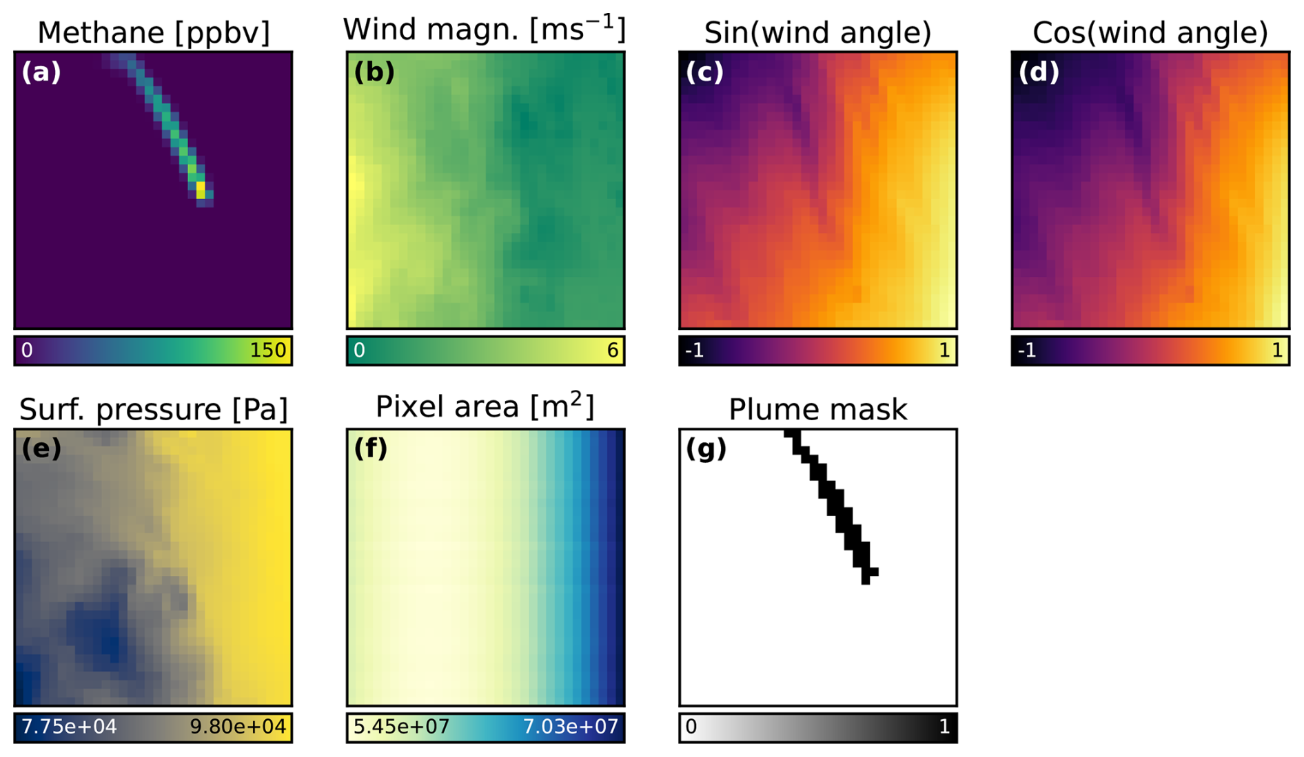
Figure 1 Channels used for input to ML-SPERE. All channel dimensions are 32×32 TROPOMI pixels. (a) Methane channel. For training and validation data, resampled plume abundances are provided, but test dataset methane scenes must be background-reduced and masked to zero outside of the defined plume mask as described in Sect. 2.2 and shown in Fig. 2. (b–d) Wind vector information, split over three channels. (e) Surface pressure. (f). Pixel area. (g) Binary plume mask. Prior to input to ML-SPERE, each of the seven channels is standardized independently using channel-wise statistics (mean and standard deviation) computed across all training images.

2.2 Test dataset creation

We evaluate our final trained model using a test set of synthetic TROPOMI methane plumes simulated with the HYSPLIT atmospheric transport model (Stein et al., 2015; Draxler and Hess, 1997, 1998; Draxler, 1999). These simulations use ERA5 global wind data (Hersbach et al., 2023a) for atmospheric transport, provided at a spatial resolution of 0.25°×0.25° and hourly temporal resolution. By constructing the test set using a different atmospheric transport code and meteorological inputs than those used for training, we assess the robustness of the model to changes in underlying plume transport representations. To further assess geographic generalization, we simulate test set plumes at multiple timestamps in 2019 at 224 global locations of known persistent methane emissions distinct from those used in training and validation, shown in Fig. A2. These “hotspot” locations are found using a wind-rotation methodology (Maasakkers et al., 2022b) and are reported to the International Methane Emissions Observatory (International Methane Emissions Observatory, 2026). The simulated plumes were scaled with emission rates matching the distribution described in Sect. 2.1 and processed identically to the training set, but without data augmentation (e.g. scaling or rotation). The final test set comprises 438 synthetic plumes.

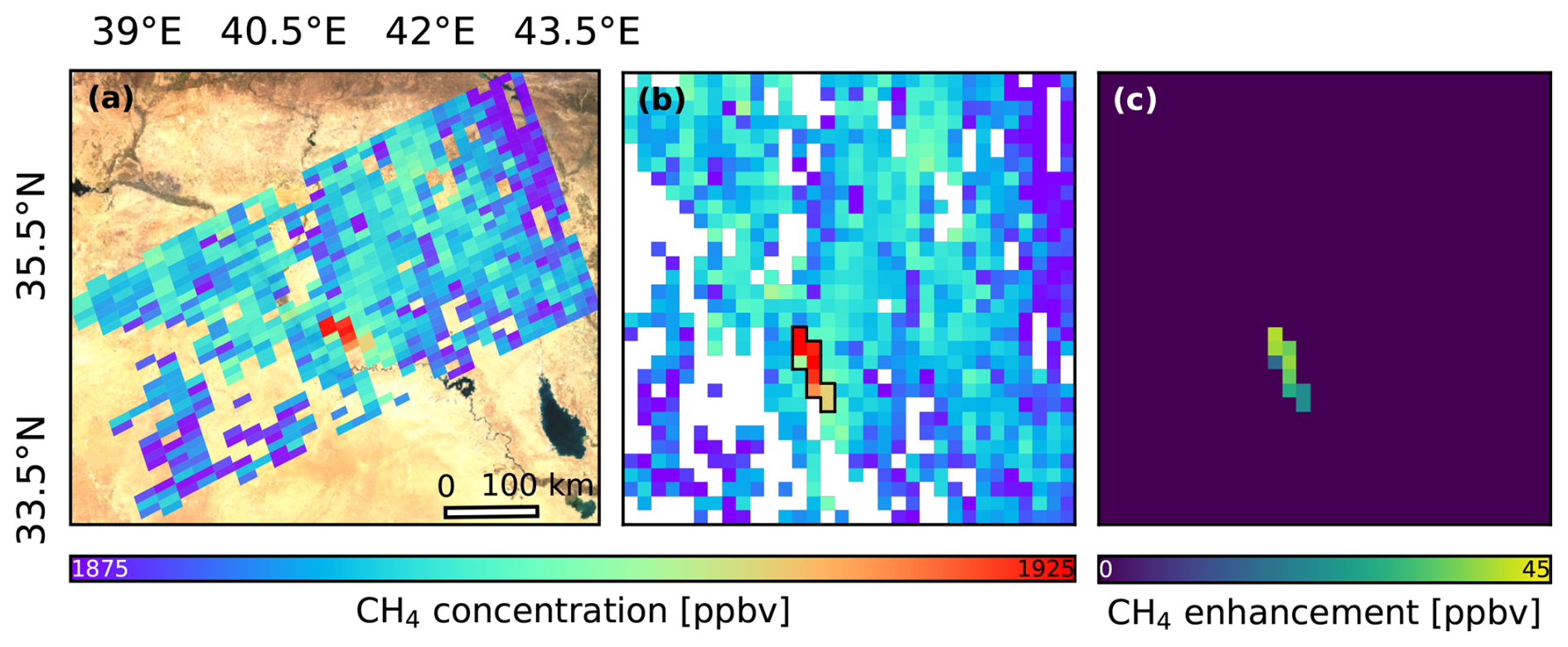
Figure 2 (a) simulated TROPOMI methane plume observation used in the test dataset, created as described in Sect. 2.2. These simulated observations combine spatially resampled HYSPLIT plumes with real TROPOMI plume-free observations to create realistic synthetic observational data, complete with realistic spatial distributions of missing data. In (b), the black outline shows the corresponding high-confidence plume mask. Valid pixels outside of this plume mask are used to estimate a background methane value for the scene. To produce the processed methane channel shown in (c), each pixel within the high confidence plume mask is background-reduced, and pixels outside of the plume mask are set to 0. This scene is passed to the CNN along with other supplementary channels after standardization (i.e. c is used as the first channel in Fig. 1). Background imagery in (a) relies on non-concurrent Sentinel-2 data (2022) adapted from Google Earth Engine (Gorelick et al., 2017; European Union, 2026).

To enhance the representativeness of the test set scenes and capture the challenges involved in estimating methane enhancements in TROPOMI data, we add a unique 32 pixel×32 pixel TROPOMI observation as background methane to each scene (Jongaramrungruang et al., 2022; Bruno et al., 2024). Using TROPOMI observations as backgrounds also introduces a realistic spatial distribution of missing data in the methane scene. These background scenes are selected from TROPOMI orbits from 2023 and 2024 using the method of Schuit et al. (2023a) to ensure they are highly unlikely to contain any real plumes. After combining a simulated plume with a randomly selected TROPOMI background scene, we pass the final scene back through the plume detection pipeline of Schuit et al. (2023a) to ensure that the synthetic plume is “detectable”. An example of a synthetic methane plume observation, complete with a real TROPOMI background methane and realistic missing spatial data, is shown in Fig. 2a. As ML-SPERE is trained using methane plume enhancements, the background methane column must be removed from the test set scenes before being used as input. We perform background removal using the binary high-confidence plume mask that is generated as part of the plume detection pipeline of Schuit et al. (2023a). First, the median methane value is calculated from pixels outside the plume mask and subtracted from all pixels in the plume mask. Then, pixels outside the plume mask are set to zero (Fig. 2b and c). We report model performance on this test set as the primary benchmark before evaluating results on real TROPOMI observations.

2.3 Model optimization and training

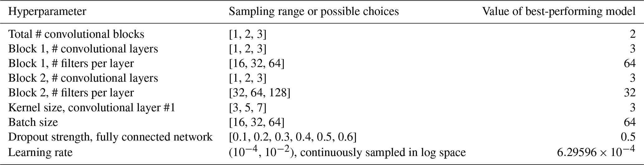
We develop and train ML-SPERE using TensorFlow (Abadi et al., 2015), a widely used machine learning framework in Python. Prior to training, both the training and validation sets are standardized on a per-channel basis relative to the training set, i.e. for each channel in an input image, values are transformed to have zero mean and unit variance based on the channel-wise mean and standard deviation of the training data. For hyperparameter optimization, we employ the Keras Tuner library (O'Malley et al., 2019) to perform a randomized grid search, fitting multiple models to the training data across a range of hyperparameter configurations. From this ensemble, we select the architecture and hyperparameters of the top-performing model, detailed in Sect. A2. The selected model architecture is relatively shallow compared to standard benchmark CNNs such as ResNet and ImageNet (He et al., 2016; Krizhevsky et al., 2017), which is expected given the relatively small image size of the input scenes and is consistent with findings in previous work (e.g. Schuit et al., 2023a), enabling efficient training that completes within a few hours on a standard desktop machine. We use the mean absolute percentage error (MAPE) as the loss function during training, chosen for its ability to reduce overfitting to high-emission scenes and provide balanced error sensitivity across the emission rate range (De Myttenaere et al., 2016; Jongaramrungruang et al., 2022; Joyce et al., 2023). Training is executed for a maximum of 100 epochs, halted early under two criteria: (1) if the validation MAPE does not improve for 10 consecutive epochs, or (2) if the ratio between the validation MAPE and training MAPE exceeds 1.05 for 10 epochs, indicating potential overfitting. ML-SPERE completed training after 18 epochs.

2.4 Emission rate uncertainty estimation

An emission rate estimate is produced by passing a processed, seven-channel input image through the trained model, which outputs a single predicted emission rate. To estimate uncertainty in these predictions, we generate an ensemble of perturbed input images that reflect both variability in pre-processing steps known to introduce uncertainty as well as uncertainty on the input data itself. By passing this ensemble through the model and analyzing the resulting emission rate distribution, we obtain an estimate of the prediction uncertainty. Our perturbation ensemble incorporates uncertainty from three primary origins: the processing required to convert a TROPOMI methane scene into a plume abundance scene, uncertainty in the wind speed, and uncertainty associated with the trained model itself.

There are two sources of uncertainty introduced during the processing of the methane channel: the method used to generate the plume mask, and the procedure for calculating methane enhancements above the local background (which is conditional on the definition of the plume mask). To address this, we first generate a binary plume mask following the procedure outlined in Schuit et al. (2023a). To account for uncertainty in this masking step, the methane scene standard deviation thresholding factor (ordinarily taken to be 1.8) is drawn from the normal distribution 𝒩(1.8, 0.2). Once the plume mask is defined, background removal is applied to the methane channel as described in Sect. 2.2. To incorporate uncertainty in the estimation of the local background methane level, we calculate the mean (${\mathit{\mu }}_{{\mathrm{CH}}_{\mathrm{4}}}$) and standard deviation (${\mathit{\sigma }}_{{\mathrm{CH}}_{\mathrm{4}}}$) of methane values in pixels outside the plume mask, excluding outliers beyond 1.5 times the interquartile range. A random background value is then sampled from the distribution $\mathcal{N}({\mathit{\mu }}_{{\mathrm{CH}}_{\mathrm{4}}},{\mathit{\sigma }}_{{\mathrm{CH}}_{\mathrm{4}}})$, capturing scene-specific uncertainty in background removal. We adopt this background reduction approach because it is more conservative (i.e. it yields a larger estimate of background uncertainty) than defining background uncertainty as the standard error of the mean of background pixels or propagating the TROPOMI retrieval uncertainties on those pixels to the background mean.

To account for uncertainty in the wind speed channels, we first compute the average wind speed $\stackrel{\mathrm{‾}}{w}$ across all pixels within the identified plume mask. If $\stackrel{\mathrm{‾}}{w}>\mathrm{3}\mathrm{m}{\mathrm{s}}^{-\mathrm{1}}$, we assign a fractional wind speed uncertainty of ${\mathit{\sigma }}_w=\frac{\mathrm{1.5}\mathrm{m}{\mathrm{s}}^{-\mathrm{1}}}{\stackrel{\mathrm{‾}}{w}}$, using the standard deviation between in-situ airfield wind speed measurements and wind data shown in Varon et al. (2018). For lower wind speeds ($\stackrel{\mathrm{‾}}{w}<\mathrm{3}\mathrm{m}{\mathrm{s}}^{-\mathrm{1}}$), we set a constant fractional uncertainty value of σ_w=0.5 (i.e. 50 % uncertainty). To incorporate this uncertainty into our ensemble of input images, we draw a wind scaling factor w_scale from a truncated normal distribution 𝒩(1, σ_w), and scale all pixel values in the wind magnitude channel by this factor. The usage of a truncated normal distribution ensures that w_scale is never negative.

A final source of uncertainty in our model's emission estimates stems from the model itself. To quantify this, we use Monte Carlo dropout as an approximation of Bayesian model uncertainty (Gal and Ghahramani, 2016). For each perturbed input image in the ensemble, we perform a single forward pass with dropout activated at inference time (dropout strength as detailed in Sect. A2). This introduces model-based variability into the total uncertainty estimate for methane plume emissions. We repeat the entire procedure (including random generation of the plume mask, methane background threshold, wind scaling factor, and a forward pass with Monte Carlo dropout) 5000 times per scene to ensure that the ensemble is sufficiently sampled. This yields a posterior distribution of emission estimates, from which we compute summary statistics such as the mean, median, standard deviation, and 2.5th and 97.5th percentiles. Unless otherwise indicated, we report the uncertainty on the estimate as the standard deviation of the posterior distribution of emission estimates. To assess the contribution of each uncertainty source, we also generate posterior distributions while systematically omitting one of the four error components.

2.5 IME method overview

We compare the performance of ML-SPERE in estimating TROPOMI methane plume emission rates with that of the IME method. In the IME method (Varon et al., 2018), the emission rate Q is estimated as

$$\begin{array}{}\text{(1)}& {\displaystyle }{\displaystyle }Q={\displaystyle \frac{U_{\text{eff}}}{L}}\text{IME}\left[\mathrm{kg}{\mathrm{s}}^{-\mathrm{1}}\right],\end{array}$$

where L [m] is the effective plume length (typically calculated as the square root of the area of the plume mask), IME [kg] is the total methane enhancement above the background summed over the plume mask, and U_eff [m s⁻¹] is the effective wind speed. Effective wind speed calibrations are specific to the instrument and can also vary according to which wind data products are used in the calibration. The effective wind speed calibration for TROPOMI as calculated from a 10 m wind speed (U₁₀) is determined in Schuit et al. (2023a) as

$$\begin{array}{}\text{(2)}& {\displaystyle }{\displaystyle }{U}_{\text{eff}}=\mathrm{0.59}{U}_{\mathrm{10}}+\mathrm{0.0}\left[\mathrm{m}{\mathrm{s}}^{-\mathrm{1}}\right],\end{array}$$

whereas the effective wind speed calibration for a planetary boundary layer average wind speed (U_PBL) is given as

$$\begin{array}{}\text{(3)}& {\displaystyle }{\displaystyle }{U}_{\text{eff}}=\mathrm{0.47}{U}_{\text{PBL}}+\mathrm{0.31}\left[\mathrm{m}{\mathrm{s}}^{-\mathrm{1}}\right].\end{array}$$

Schuit et al. (2023a) calculate Q using ERA5 10 m winds (Hersbach et al., 2023b) as well as GEOS FP 10 m and planetary boundary layer winds (Molod et al., 2012). They additionally estimate uncertainties using a grid-based ensemble approach, varying input parameters such as plume masking thresholds, background methane concentration, wind magnitudes, and effective wind speed coefficient values. IME estimates (and associated uncertainties) for synthetic and real methane observations in this work follow the methods of Schuit et al. (2023a) directly, using only the ERA5 10 m wind product. We apply the IME method and U_eff parameterization from Schuit et al. (2023a) without modification, allowing us to benchmark the performance of ML-SPERE against a published and operationally used implementation of the IME method that was specifically calibrated for TROPOMI methane observations.

3 Results

After optimizing and training our model, we evaluate its performance on a test set of synthetic methane plume observations (Sect. 3.1). Because the true emission rates are known, we can assess ML-SPERE under a range of scenarios and examine its performance. Next, we apply our model to a well-studied blowout, enabling evaluation of its estimates against both inverse modeling approaches and the IME method using data from TROPOMI and higher-resolution satellites (Sect. 3.2). Finally, we use ML-SPERE to quantify the emission rates of an entire year's worth of TROPOMI super-emitter detections (Sect. 3.3).

3.1 Test set evaluation and comparison to the IME method

We evaluate ML-SPERE performance using the global test set of synthetic TROPOMI methane plume observations generated with HYSPLIT (Sect. 2.2). On this test set, ML-SPERE achieves a MAPE of 40.2 %, compared to 46.1 % for the IME method, as shown in Fig. 3. Notably, the median absolute percentage error (MdAPE) for IME estimates is 40.5 %, while ML-SPERE yields a substantially lower MdAPE of 29.5 %. This difference arises because ML-SPERE estimates for this test set exhibit a heavy-tailed error distribution (arising from scenes where the plume is poorly observed, see following paragraph), and metrics such as MAPE are strongly influenced by outliers. Absolute errors produced by ML-SPERE generally scale with the true emission rate of test set plumes, but this relationship breaks down at the lowest emission rates, where an approximately constant absolute error leads to inflated relative errors. Similar behavior is observed for IME estimates. Additional performance metrics such as the Pearson correlation coefficient (R), mean absolute error (MAE), median absolute error (MdAE), mean bias, and root mean squared error (RMSE) are summarized in Table 1. We find no significant change in bias for either method when applied only to plumes whose masks are truncated by the scene boundary. Across all metrics, ML-SPERE outperforms the IME method. In terms of computational efficiency, the IME method implementation from Schuit et al. (2023a) is faster than ML-SPERE. On a standard desktop machine, it takes approximately 15 s to generate either an ensemble estimate of 43 923 members with the IME method or an ensemble estimate of 5000 members with ML-SPERE. These timings may vary depending on hardware. The time it takes ML-SPERE to produce an ensemble estimate scales linearly with the number of ensemble members.

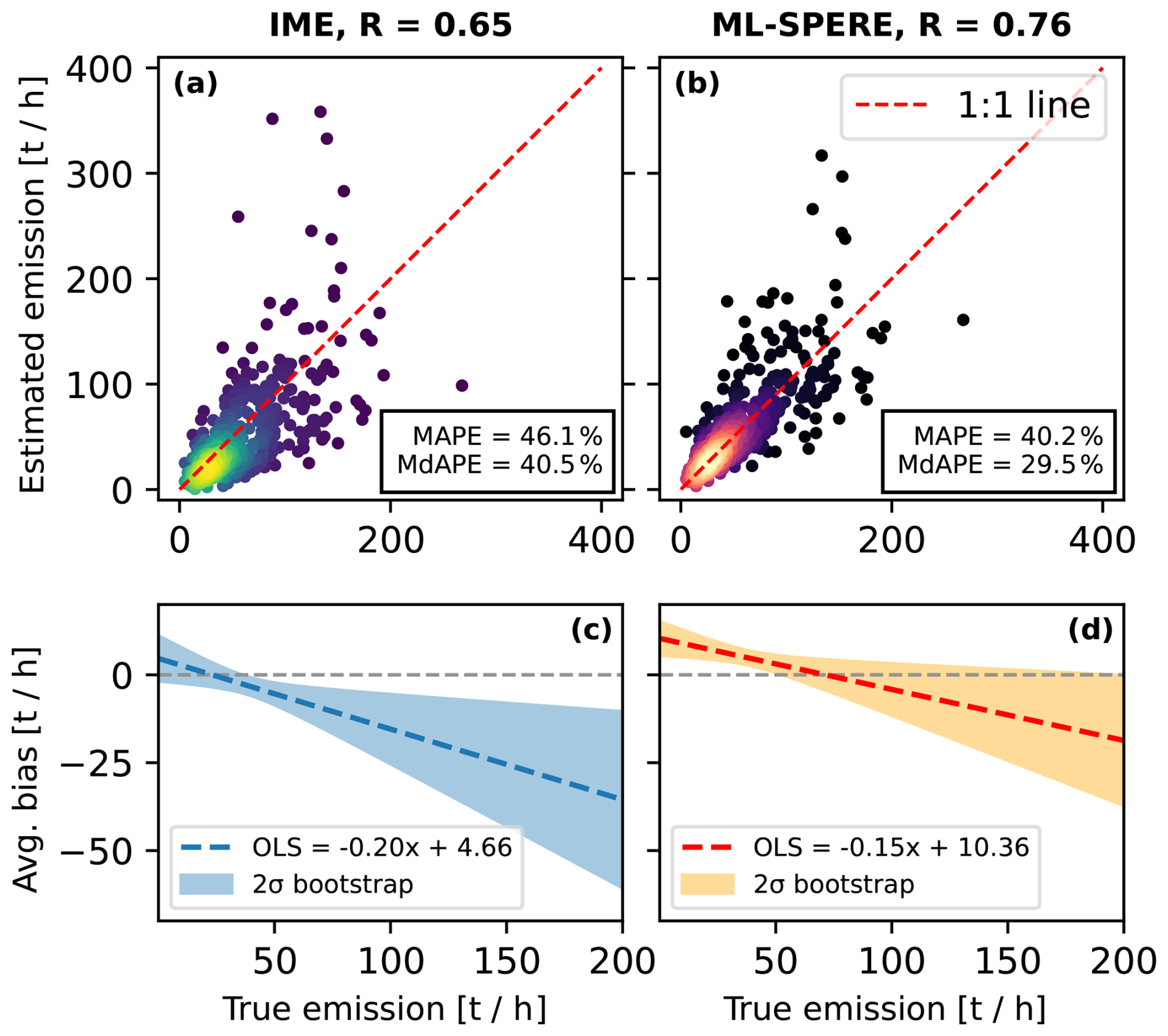
Figure 3 Estimated emission rates for the test set of HYSPLIT plumes via (a) the IME method and (b) ML-SPERE as a function of true plume emission rates. The colormaps represent the relative density of the visualised data. We visualise bootstrapped ordinary least squares (OLS) regression lines for emission rate estimates from both the IME method (c) and ML-SPERE (d). The 1:1 line is subtracted in (c) and (d) to show average bias for each method across the entire range of emission rates of test set plumes. The regression dilution apparent in panel (d) for ML-SPERE is partially alleviated when application is limited to well observed plumes, see Fig. A4d.

Table 1 Comparison of performance metrics for the IME method and ML-SPERE emission rate estimation when evaluated on the test set (Sect. 3.1). Best performance for each metric is shown in bold. Metrics shown are Mean Absolute Percentage Error (MAPE), Median Absolute Percentage Error (MdAPE), Pearson correlation coefficient (R), mean absolute error (MAE), median absolute error (MdAE), mean bias, and root mean squared error (RMSE). In the first two rows, we compare results for the two methods across the entire test set (438 plumes), and in the second two rows, we compare results for the two methods for well-observed scenes only (264 plumes), testing only against plumes where the emission source location is contained within the estimated plume mask. We also include the performance of both methods only for plumes which are poorly observed in the last two rows (174 plumes).

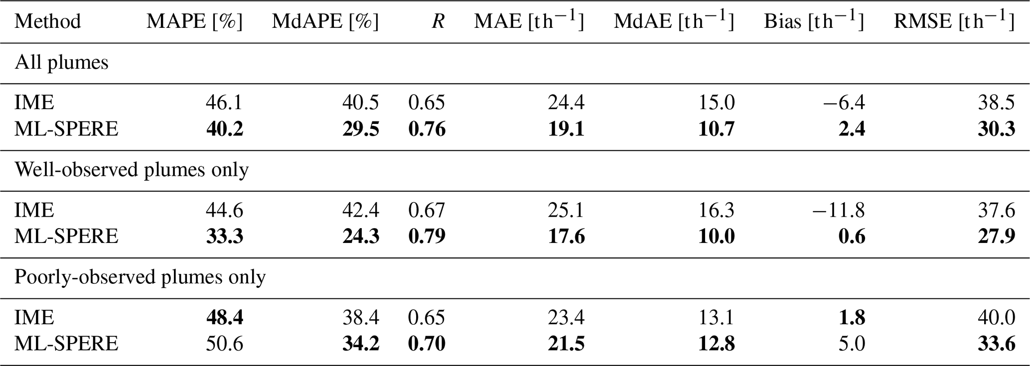
The construction of plume masks is complicated by missing data and high methane background variability (various examples are shown in Fig. A3). We thus define a TROPOMI methane plume in the test set to be “well-observed” if the known emission source location is contained within the estimated plume mask. When filtering the test set to include only scenes where the plume is well-observed (resulting in 264 scenes), the performance gap between ML-SPERE and the IME method widens further (Table 1). MAPE and MdAPE of ML-SPERE decrease to 33.3 % and 24.3 %, respectively, whereas the corresponding IME errors remain largely unchanged at 44.6 % and 42.4 % (Fig. A4). Additional figures and analyses in Sect. A3 show that the improved performance observed when restricting the application of ML-SPERE to such plumes arises from the model's strong reliance on spatial gradients in methane abundance near the plume head or source region when inferring emission rates. This behavior lends ML-SPERE meaningful physical interpretability. Performance may degrade when the plume mask is compromised around the plume head, either by missing data or by methane enhancements that are weak relative to background variability. However, such conditions are generally visually identifiable, allowing for informed application of the model. Even when the source location is unknown, an analyst can inspect a scene to assess whether the estimated plume mask is compromised and, consequently, whether ML-SPERE is likely to provide a reliable emission estimate. For poorly-observed plumes in the test set (i.e. those that do not meet the criteria for being well-observed), ML-SPERE and the IME method exhibit broadly comparable performance. ML-SPERE performance degrades relative to its results on well-observed plumes, whereas IME performance remains similar across all subsets.

While ML-SPERE achieves a MAPE of 40.2 % on the full test set and 33.3 % on well-observed plumes, its performance on the validation set is substantially better, with a MAPE of 14.6 %. Significant differences between the validation (and training) set and the test set include the fact that the validation set contains no spatially varying backgrounds or missing data, and that the validation set was simulated using WRF-Chem with NCEP wind data, which matches the modeling framework used for training. The test set plumes are additionally simulated at a wide variety of locations around the globe which are distinct from the locations used for model training. We have already demonstrated that spatially varying backgrounds and missing data hamper the performance of ML-SPERE by complicating the estimation of accurate plume masks. In Sects. A5 and A6, we demonstrate that further performance degradation on the test set (with respect to validation set performance) arises primarily from the use of HYSPLIT to generate test plumes, which exhibit morphologies distinct from those produced by WRF-Chem and encountered during training, rather than from limitations in geographic generalization.

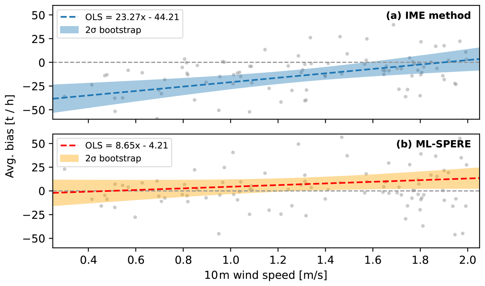
Figure 4 Estimate bias (expressed as the residual between an emission rate estimate for a method and the true emission rate) for HYSPLIT test set plumes, estimated via the IME method (a) and ML-SPERE (b) as a function of 10 m wind speeds. Also shown are ordinary least square regressions for both datasets. Due to the linear calibration of the effective wind speed to the input 10 m wind speed, the IME estimate residuals show a strong negative bias at low wind speeds, however ML-SPERE yields unbiased estimates at wind speeds below 2 m s⁻¹.

Figure 3 illustrates a systematic bias where ML-SPERE tends to underestimate emission rates for plumes with large emission rates above the mean of the training dataset, and overestimate emission rates for plumes with small emission rates below the mean. The IME method also tends to underestimate emissions for plumes with large emission rates, despite the fact that the IME method is not a mean-biased method. The tendency for ML-based predictions to regress toward the mean of the training dataset labels is a common issue reported in similar studies (Jongaramrungruang et al., 2022; Joyce et al., 2023; Bruno et al., 2024). This regression dilution for ML-SPERE is reduced by $\mathrm{1}/\mathrm{3}$ when we restrict application to well-observed plumes (Fig. A4d), though no such improvement in estimate biases is found for the IME method (Fig. A4c). For scenes with wind speeds below 2 m s⁻¹, residuals between ML-SPERE emission rate estimates and true plume emission rates show no correlation with scene wind speed. In contrast, residuals of IME estimates in this wind speed regime exhibit a strong positive correlation, with the IME method significantly underestimating emissions for these plumes. Although low wind speeds aid in plume detection (48 % of the detections reported by Schuit et al. (2023a) are found at wind speeds below 2 m s⁻¹), they complicate emission rate quantifications for mass-balance based approaches such as the IME method and the cross-sectional flux (CSF) method (Krings et al., 2011, 2013). Under such conditions, plumes often exhibit blob-like structures or irregularly rotated morphologies (Pandey et al., 2023), which complicate emission rate estimation. Equation (1) in conjunction with the 10 m effective wind speed calibration from Eq. (2) implies that as U₁₀ approaches zero, the IME-estimated emission rate Q must also approach zero. As a result, the IME method may be biased low and underestimate emissions from methane plumes detected by TROPOMI in low-wind-speed environments, for which the uncertainty on the wind speed is also relatively large. Figure 4 shows this trend clearly, and displays that the IME method systematically underestimates the emission rates for test set plumes with average wind speeds of less than 2 m s⁻¹. By contrast, ML-SPERE is an unbiased estimator for plumes at low wind speeds, despite utilizing the same input data as the IME method.

Ideally, a model that accurately estimates uncertainty would capture about 95 % of true emission values within the 2.5th–97.5th percentile range of its posterior distribution for each emission-rate estimate. Across the full test set, 61 % of true values fall within this interval for IME estimates, compared to 81 % for ML-SPERE. These results indicate that both methods underestimate predictive uncertainty, although ML-SPERE provides more reliable uncertainty estimates than the IME method. We retain the hyperparameters specified in the error ensemble described in Sect. 2.4 (i.e. the assumed uncertainties in wind speeds, methane backgrounds, and plume masking strength) which are drawn from literature or informed by expert judgment. While increasing these values could widen the estimated uncertainty ranges (and thereby increase the proportion of true emission rates captured within them), doing so would risk masking model misspecification by attributing errors to input uncertainty alone. In Sect. A4 and Fig. A6, we apply the probability integral transform to show that the ML-SPERE error ensemble generalizes better across simulated plume datasets than the IME approach.

3.2 Case study comparison: Kazakhstan's Karaturun East oil field 2023 blowout

In 2023, a well blowout took place in Kazakhstan's Karaturun East oilfield which lasted for more than 200 d (days) (Guanter et al., 2024). This event was observed with multiple methane-sensing satellites, including TROPOMI and high-resolution (25–60 m) satellite instruments such as GHGSat (Varon et al., 2019; Jervis et al., 2021), EMIT (Thorpe et al., 2023), EnMAP (Roger et al., 2024), and PRISMA (Guanter et al., 2021). For TROPOMI methane observations, inverse analysis estimates of emission rates were produced on a daily basis when observing conditions allowed. Separate IME estimates were also made using the observations of the point-source imagers when available. These quantifications showed that the daily estimated emission rate varied between 20–50 t h⁻¹ over the duration of the blowout, emitting an estimated total of 131±34 kt of methane (Guanter et al., 2024). For dates during this blowout where a methane plume is detected in the TROPOMI data following the procedure of Schuit et al. (2023b), we compare ML-SPERE emission rate estimates with those from Guanter et al. (2024) as well as to IME emission rates estimates that we have produced using the TROPOMI data.

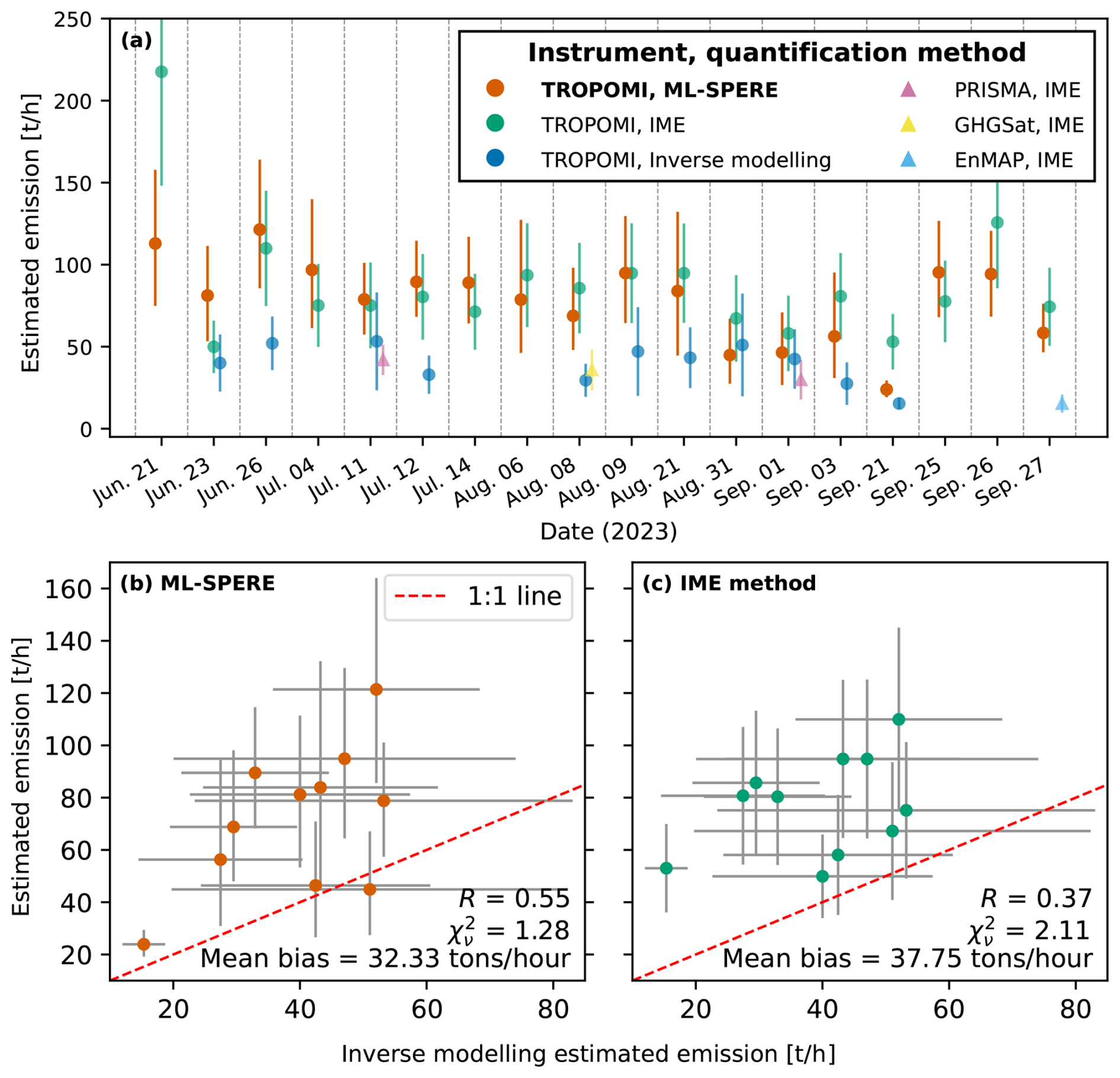
Figure 5 (a) Time series of daily estimated methane emission rates emission rates for the Karaturun East oilfield blowout. TROPOMI inverse modeling estimates and high-resolution satellite IME estimates are taken from Guanter et al. (2024). ML-SPERE data points are median values of the estimated posterior distribution of estimated emissions. Errorbars shown are ±1σ, with the exception of error bars for ML-SPERE estimates, which extend from the 16th to the 84th percentile of the posterior distribution of emission estimates (all statistics are given in Table A3). We choose to represent error bars for ML-SPERE with percentiles to show the skewed shape of the posterior distribution of the estimate (e.g. see Fig. A6a). (b) ML-SPERE estimates of the daily emission rate compared to the TROPOMI inverse modeling estimate for that same day. (c) IME estimates of the daily emission rate compared to the TROPOMI inverse modeling estimate for that same day.

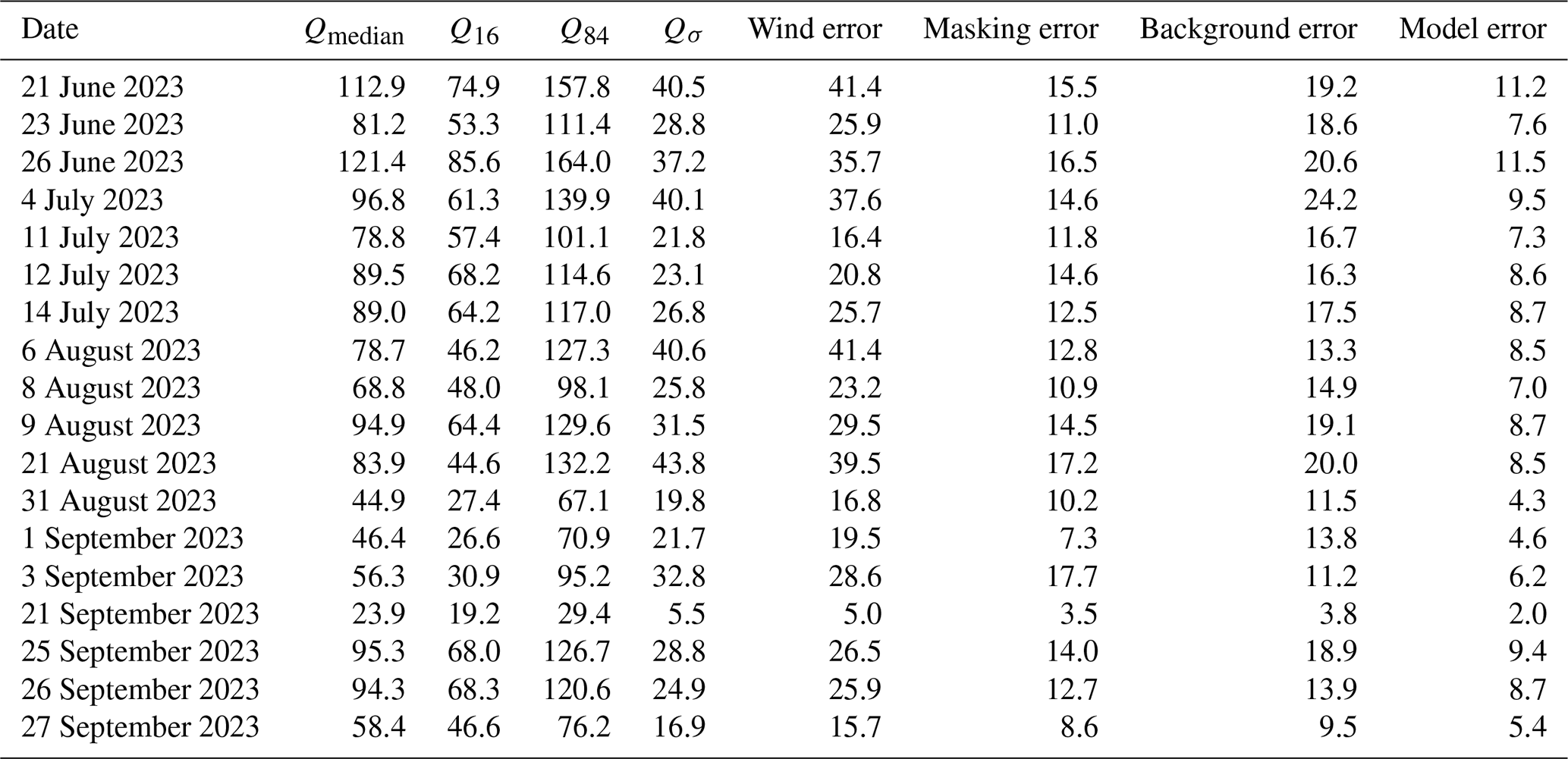
Figure 5a shows a time series of the daily emission rate estimates from Guanter et al. (2024) and the ML-SPERE estimates. In general, ML-SPERE estimates tend to be higher than the TROPOMI inverse modeling results presented in Guanter et al. (2024), although they typically agree within uncertainty and show slightly closer agreement than that between the TROPOMI inverse modeling and IME estimates. For three of the four dates in the time series where we have an IME emission rate estimate from a high-spatial resolution satellite, we find greater agreement with ML-SPERE estimates than we do with TROPOMI IME estimates. We also find general agreement between ML-SPERE estimates and TROPOMI IME estimates. Error bars in Fig. 5 for ML-SPERE estimates span from the 16th to the 84th percentile of the posterior distribution of emission rates, in order to show the skew of posterior estimates (e.g. see Fig. A6a). These error bars are typically skewed with a heavy tail toward higher emission values, since ML-SPERE will not produce estimates below zero but has no upper bound. For most days in the time series, the uncertainty in ML-SPERE predictions is dominated by uncertainty in the input wind data. The next largest contribution to the overall uncertainty arises from uncertainty in estimating the methane background level within each scene. In contrast, uncertainties associated with plume masking and the model itself contribute comparatively little to the total uncertainty (Table A3).

In Fig. 5b and c, we compare ML-SPERE estimates and TROPOMI IME estimates with the corresponding TROPOMI inverse modeling estimates. The ML-SPERE estimates exhibit a reduction in bias relative to the TROPOMI IME estimates when compared against the inverse modeling results, along with an improved R correlation and reduced chi-squared ${\mathit{\chi }}_{\mathit{\nu }}^{\mathrm{2}}$ (though the scatter between inverse analysis estimates and both ML-SPERE and TROPOMI IME estimates remains large). To investigate potential sources of bias between ML-SPERE and the inverse modeling estimates for these scenes, we apply ML-SPERE directly to the resampled simulated plumes from Guanter et al. (2024) that were identified as the best matches to the observations. Using these simulated plumes (without missing data or background methane) and their corresponding meteorology as inputs, ML-SPERE shows improved agreement with the simulated emission rates (i.e. the results shown in Guanter et al., 2024), achieving a Pearson correlation of R=0.91 and a substantially reduced mean bias of 15.4 t h⁻¹. In contrast, IME estimates applied to the same simulated plumes remain largely unchanged relative to the metrics shown in Fig. 5c. The remaining positive bias of 15.4 t h⁻¹ in the ML-SPERE estimates could be attributable to plume morphologies resulting from complicated wind fields or conditions which violate the steady-state emission assumptions represented in the training dataset. This interpretation is supported by the fact that the IME method (which assumes steady-state emission scenarios) produces estimates that are twice as large as those of the ML-based estimates when applied to the same simulated plumes from Guanter et al. (2024). Furthermore, ML-SPERE does not show similar positive biases when applied to other simulated plume datasets with steady-state emissions (e.g. Figs. 3, A4, A7, and A8). Applying ML-SPERE to the same simulated plumes while masking the abundances to reproduce the spatial pattern of missing data in the TROPOMI observations does not degrade performance. This robustness arises because the well blowout source remains clearly visible, and the absence of a spatially variable methane background allows the automatically generated plume masks in the ML-SPERE ensemble to reliably capture the source region. These results suggest that the remaining scatter between ML-SPERE and inverse modeling estimates for the real TROPOMI observations is likely driven by a combination of highly variable coastal methane backgrounds that complicate plume masking on certain dates, discrepancies between meteorological reanalysis products and true wind vectors, and conservative inverse modeling estimates where the forward modeled plume does not closely reproduce the TROPOMI observation. Although the actual underlying emission rates are not known for this super-emitting blowout, the improved agreement between ML-SPERE and inverse modeling estimates (compared to IME method vs. inverse modeling agreement) is notable as inverse modeling is a far more information-rich method, incorporating three-dimensional wind fields and atmospheric transport processes to produce plume emission rate estimates (albeit at a substantially higher computational cost than other methods).

3.3 Population study: cataloged 2021 TROPOMI methane plume detections

Schuit et al. (2023a) present an automated, ML–based algorithm for detecting large methane emission plumes in TROPOMI satellite data, with a corresponding catalog of detections for all of 2021 published in Schuit et al. (2023b). This dataset comprises 2974 plume detections distributed globally, with all but 30 linked to dominant anthropogenic sources such as urban areas/landfills, oil, gas, or coal mining operations based on bottom-up inventories. We use this 2021 detection catalog as a benchmark dataset to compare the performance of ML-SPERE to the traditional IME approach. ML-SPERE and IME estimates exhibit a strong correlation (R=0.79, Fig. 6a) and agree within errors (${\mathit{\chi }}_{\mathit{\nu }}^{\mathrm{2}}=\mathrm{0.94}$, Fig. 6a). ML-SPERE estimates tend to exceed those of the IME method at low IME-estimated emission rates (i.e. below 10 t h⁻¹). This behavior may reflect the regression dilution discussed in Sect. 3.1 and shown in Fig. 3c. Additionally, it may indicate underestimation by the IME method for these plumes due to the wind-speed bias described in Sect. 3.1, as discussed further below. Emission estimates for TROPOMI plumes below 10 t h⁻¹ should be interpreted with caution, as this lies near the conventional detection threshold.

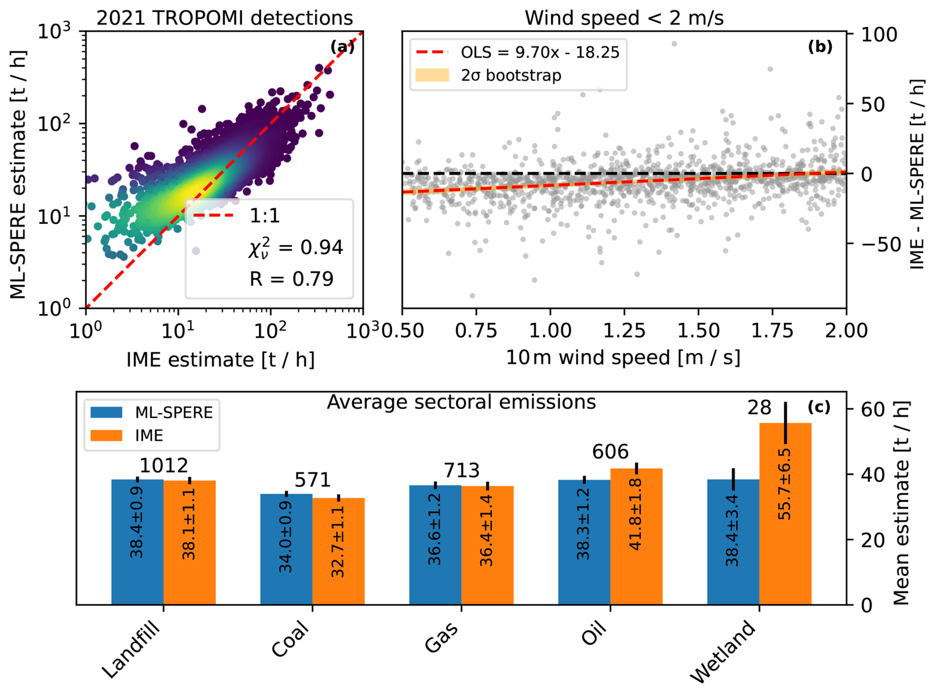
Figure 6 (a) TROPOMI 2021 methane plume detections quantified via the IME method and ML-SPERE. We quantify (and compare with the IME method) all but 44 of the 2974 scenes in Schuit et al. (2023b) with ML-SPERE. These 44 scenes had ML-SPERE ensemble members with empty plume masks, due to combinations of low plume enhancements and high masking thresholds. The colormap represents the relative density of the visualised data. (b) Residuals between IME emission rate estimates and ML-SPERE emission rate estimates as a function of scene 10 m wind speed, for detected TROPOMI plumes for 2021 with scene wind speeds below 2 m s⁻¹. This trend in residuals shown here could be explained by unbiased estimates from ML-SPERE as a function of scene wind speed, and biased estimates from the IME method that grow increasingly negative with decreasing scene wind speed. (c) Plume emission rates averaged across estimated sectoral classification. Total number of plumes per estimated sector is printed above each grouping, and mean estimated emissions are printed within each bar. Errorbars are standard errors on the mean.

As shown in Sect. 3.1 and Fig. 4, ML-SPERE produced unbiased estimates with no correlation with wind speed for low-wind plumes in the synthetic test set, while the IME method showed increasing negative bias with decreasing wind speed. The residuals between the IME estimates and those of ML-SPERE for the real 2021 plume dataset exhibit a similar trend at lower wind speeds (Fig. 6b), which is consistent with the findings from Sect. 3.1. As nearly half of plumes are detected at wind speeds below 2 m s⁻¹, ML-SPERE may therefore provide less biased emission rate estimates than the IME method for these commonly detected plumes.

A global comparison of ML-SPERE and IME emission rate estimates for the full 2021 TROPOMI detection catalog reveals that although the two methods generally agree (Fig. 6a), there are few regions where systematic differences emerge. These differences are statistically significant only in northern Russia and southwestern Australia, where ML-SPERE yields higher estimates than the IME method, and in the Congo Basin, where ML-SPERE yields lower estimates. A full analysis is given in Sect. A8 (with Figs. A9 and A10) and summarized below.

In northern Russia, the largest discrepancies correspond to extremely compact, high-enhancement signals that coincide spatially with major gas pipeline infrastructure. These features resemble short-duration, transient emissions rather than the steady-state plumes on which ML-SPERE was trained, and their out-of-sample elevated methane enhancements likely contribute to the elevated emission estimates. Such transient, non steady-state emissions may also not be well estimated by the IME method (especially if the plume has detached from the source and is being transported downwind, as this violates the steady-state assumptions underlying the method). For these plumes, the total plume mass may provide a more relevant characterization than estimated instantaneous emission rate as emissions are no longer ongoing (De Jong et al., 2025). For ongoing or persistent events, the observed mass only provides a lower boundary for the total emitted mass, as mass is still being emitted at the time of observation. In contrast to pipeline emissions in northern Russia, methane enhancements in the Congo Basin have very large spatial extents and may be more representative of area-source emissions than (TROPOMI-scale) point-source emissions on which ML-SPERE was trained and the IME method was calibrated. Finally, for plumes in southeastern Australia, ML-SPERE estimates are systematically higher than IME estimates in a low–wind-speed regime, where we have already demonstrated that IME estimates exhibit a negative bias. Although transient emission events and spatially extended plumes can occur globally, analysis of this dataset suggests that temporal averaging limits statistically significant differences between total emissions estimated by the two methods to a small number of regions. These regional diagnostics highlight that ML-SPERE likely performs most accurately when the observed plume exhibits a coherent head and well-defined downwind structure, and that applying either method can benefit from human oversight in cases involving transient, discontinuous emissions or spatially fragmented plumes.

In Fig. 6c, we compare average estimated emissions for the 2021 TROPOMI plume detections grouped by estimated source sector (Schuit et al., 2023b). Sectoral emissions estimated for this dataset using the IME method and ML-SPERE largely agree, with the exception of those attributed to wetland emissions, which are underrepresented in this dataset. These plumes are spatially concentrated in the Congo Basin and, as discussed in the previous paragraph, have large spatial extents that may lead to overestimation by the IME method. The agreement across the remaining sectors likely reflects averaging over a broad distribution of wind speeds, which can mitigate wind-speed–dependent biases in the IME method. Taken together, the consistency between ML-SPERE and IME across most sectors supports the robustness of the sectoral emission estimates for this plume dataset.

4 Conclusions

This study presents ML-SPERE, an ML-based method for quantifying emission rates of methane plumes detected in TROPOMI observations. We trained ML-SPERE using synthetic TROPOMI methane plumes, which were simulated using WRF-Chem and then resampled to TROPOMI pixel footprints. Wind data was also included in the training dataset. We additionally used HYSPLIT to simulate a test set of methane plumes at locations not included in the training data. This test set is global and includes real TROPOMI methane scenes as backgrounds, which introduces realistic challenges in reducing methane scenes to plume abundances. We evaluate ML-SPERE against this synthetic test set, and additionally use ML-SPERE to quantify the emission rates of real TROPOMI methane plumes observed during a well-studied blowout in Kazakhstan, as well as for an entire year's worth of automated super-emitter detections from 2021. At all stages of model evaluation, we benchmark the performance of ML-SPERE against that of the IME method.

When evaluating emission rate estimates produced by ML-SPERE for the full synthetic test set and comparing them to those from the IME method, we find that MAPE improves from 46.1 % to 40.2 %, MdAPE improves from 40.5 % to 29.5 %, and R improves from 0.65 to 0.76. ML-SPERE performance exceeds that of the IME method for every metric measured on the test set. ML-SPERE is found to have a regression bias across emission rates as is usually the case with ML regressors. When filtering test set scenes for plumes where we have spatially complete information around the source location and plume head, the performance gap between ML-SPERE and the IME method increases further, and metrics such as MAPE, MdAPE, R, and biases are all significantly improved for our model. We show empirically that this is because ML-SPERE has learned to use methane gradients around the plume head to inform emission rate estimates, which lends ML-SPERE clear physical interpretability. We also find that estimates from ML-SPERE are unbiased with respect to scene wind speed, but that IME estimates are not. We demonstrate that IME estimates can be systematically underestimated for methane plumes detected at wind speeds below 2 m s⁻¹, which are conditions where real TROPOMI methane plumes are commonly detected. This ability of ML-SPERE to provide unbiased estimates in this wind regime which is favorable for plume detection represents a significant improvement for emission rate quantification for TROPOMI methane plumes.

When using ML-SPERE to quantify emissions for the 2023 Karaturun East blowout in Kazakhstan, we find that ML-SPERE estimates typically agree within uncertainties with IME and inverse analysis estimates from TROPOMI observations. Compared with TROPOMI IME estimates, ML-SPERE estimates show improved agreement with the high-resolution IME estimates. ML-SPERE estimates show a slightly reduced bias relative to TROPOMI IME estimates when compared against inverse modeling though scatter remains. ML-SPERE was further evaluated using a global catalog of TROPOMI methane plume detections from 2021, providing a comprehensive real-world benchmark against the traditional IME method. Across this dataset, ML-SPERE and IME estimates show strong general agreement (R=0.79). Critically, the 2021 detections reproduce the wind-speed sensitivity found in our simulated test set: at low wind speeds (less than 2 m s⁻¹), IME vs. ML-SPERE residuals become increasingly negatively biased, indicating that the implemented IME method may have a wind-speed dependent bias and that ML-SPERE does not show such bias. A global spatial comparison further reveals that, although agreement is generally strong, systematic regional differences arise in only a few locations and reflect scene-specific factors in addition to potential methodological limitations. In particular, scenarios in which neither the IME method nor ML-SPERE is well suited for application (e.g. violations of point-source or steady-state assumptions) likely require more careful consideration using situation-tailored approaches. Future work could examine re-training ML-SPERE using a larger dataset, with expanded geographic and seasonal diversity that focuses on regions and circumstances where we have shown that ML-SPERE and the IME method produce larger differences in emission rate estimates, though the results of Sect. A5 show that ML-SPERE generalizes beyond the spatial domain of training data. Average sectoral emissions for this dataset as estimated via the IME method or ML-SPERE are broadly unchanged, with the exception of wetland emissions, which are underrepresented in this dataset both spatially and numerically. Together, these diagnostics show that ML-SPERE performs robustly across diverse real-world conditions and particularly well in common low-wind regimes. When combined with human oversight, it offers a reliable and complementary alternative to the IME method for routine global quantification of methane emissions from TROPOMI plumes.

Appendix A: Additional material

A1 Simulated plume locations

In Fig. A1 we show the locations of the WRF-Chem domain setups and tracer release location schemes. In Fig. A2 we show the locations of the plumes simulated for the test set using HYSPLIT.

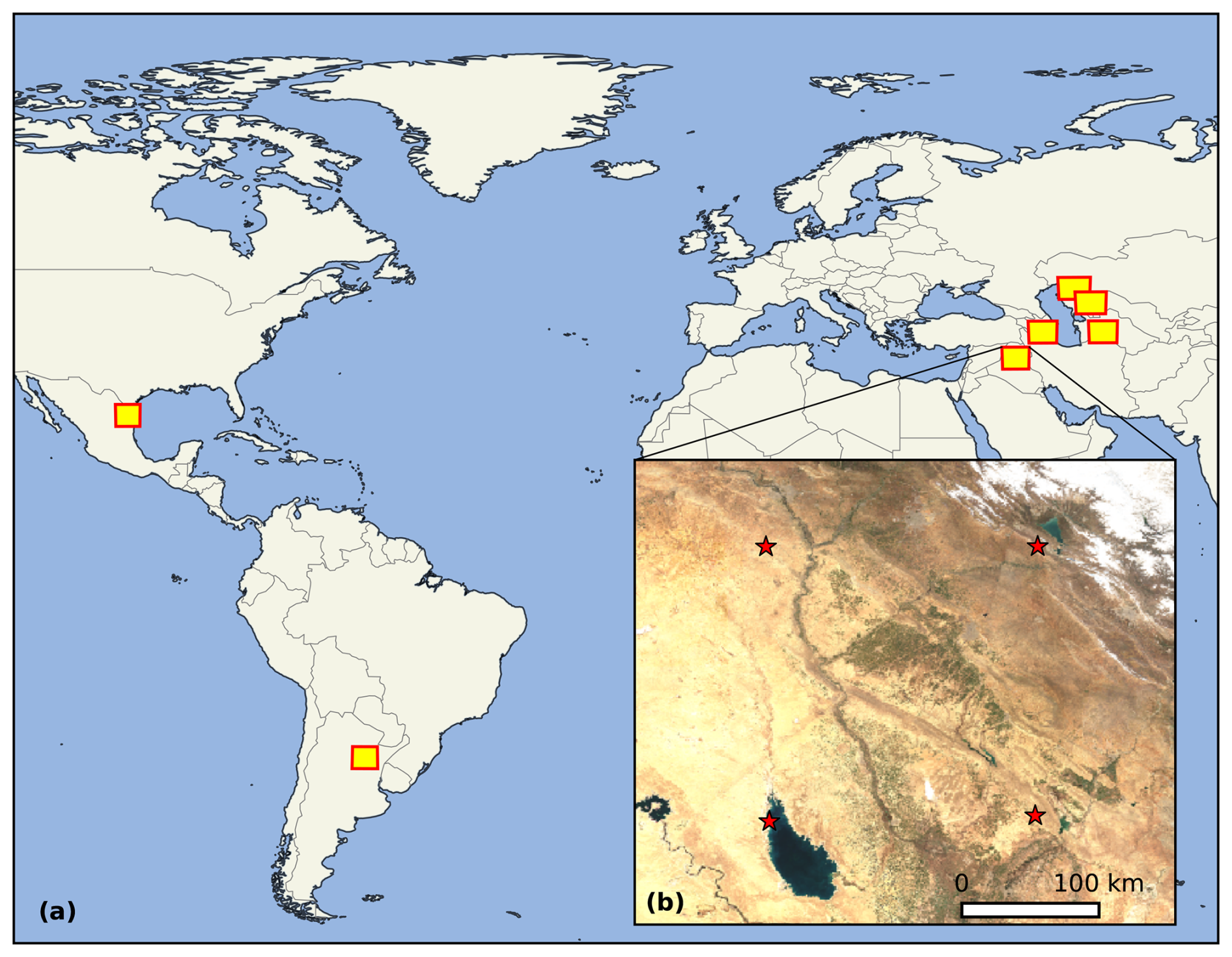
Figure A1 (a) The inner domain of the nested WRF-Chem setups, shown with the yellow rectangles. For each of these inner domains, 8 passive tracers are initialized to emit over the duration of the simulations, at 4 different locations and 2 different release heights. Tracer locations are shown with the stars in the example domain shown in (b), and at each star, tracers are initialized at approximately 25 and 250 m heights. Background imagery in (b) relies on non-concurrent Sentinel-2 data (2022) adapted from Google Earth Engine (Gorelick et al., 2017; European Union, 2026).

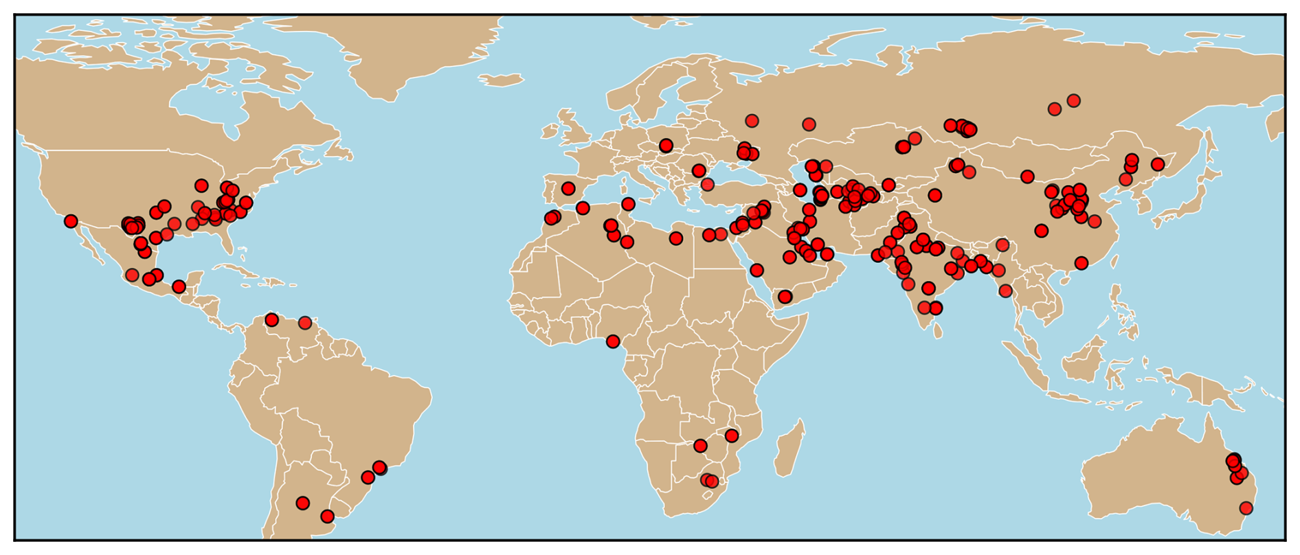
Figure A2 438 test set plumes simulated at 224 unique global locations with HYSPLIT.

A2 Model structure optimization

The class of model optimized is that of a “traditional” CNN, i.e. a series of convolutional blocks followed by a fully connected network and ending with a single output node. Each convolutional block is formed from a specified number of convolutional layers, followed by a max-pooling layer. Every convolutional layer within one block shares the same number of filters, and each convolutional layer within any block is followed by a rectified linear unit activation function. Additional model hyperparameters or design choices such as the learning rate, batch size, kernel size of the first convolutional layer, and dropout strength of the fully connected network were also optimized. Model hyperparameters were optimized by sampling hyperparameters from the choices or ranges shown in Table A1, fitting 500 models to the training and validation data described in Sect. 2.1, and choosing the best-performing model structure when evaluated on the validation dataset. Chosen hyperparameter values of the final optimized ML-SPERE are shown in the final column of Table A1.

Table A1 Sampled ranges/values for optimized hyperparameters of ML-SPERE. Hyperparameters of the final optimized model are shown in the right-most column.

A3 ML-SPERE performance under ideal observing conditions

When restricting the evaluation of ML-SPERE on the test set to only include scenes where the emission source is contained within the estimated plume mask (e.g. Fig. A3a and b), we find that our average emission estimates are greatly improved (Table 1, Fig. A4). The enhanced performance we find for ML-SPERE when restricting the test set to plumes in which the true source pixel falls within the estimated plume mask suggests that ML-SPERE relies strongly on information near the plume head or source region when inferring emission rates. This hypothesis is supported by the fact that ML-SPERE is trained on resampled plume abundance scenes without complicating backgrounds or missing spatial data (e.g. Sect. 2.1, Fig. 1), and information around the plume head is always available during training.

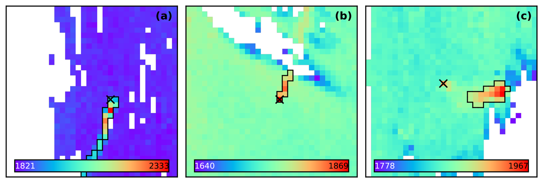
Figure A3 A few examples of test set plumes and their derived plume masks outlined in black. Emission source locations are shown with a black x. In (a), the plume is easily delineated. In (b), the head of the plume is captured, but missing data prevents the rest of the plume from being included in the mask. In (c), background variability results in only some of the plume being successfully delineated, and the source pixel is not included in the mask. Colorbar values are methane concentrations in ppbv.

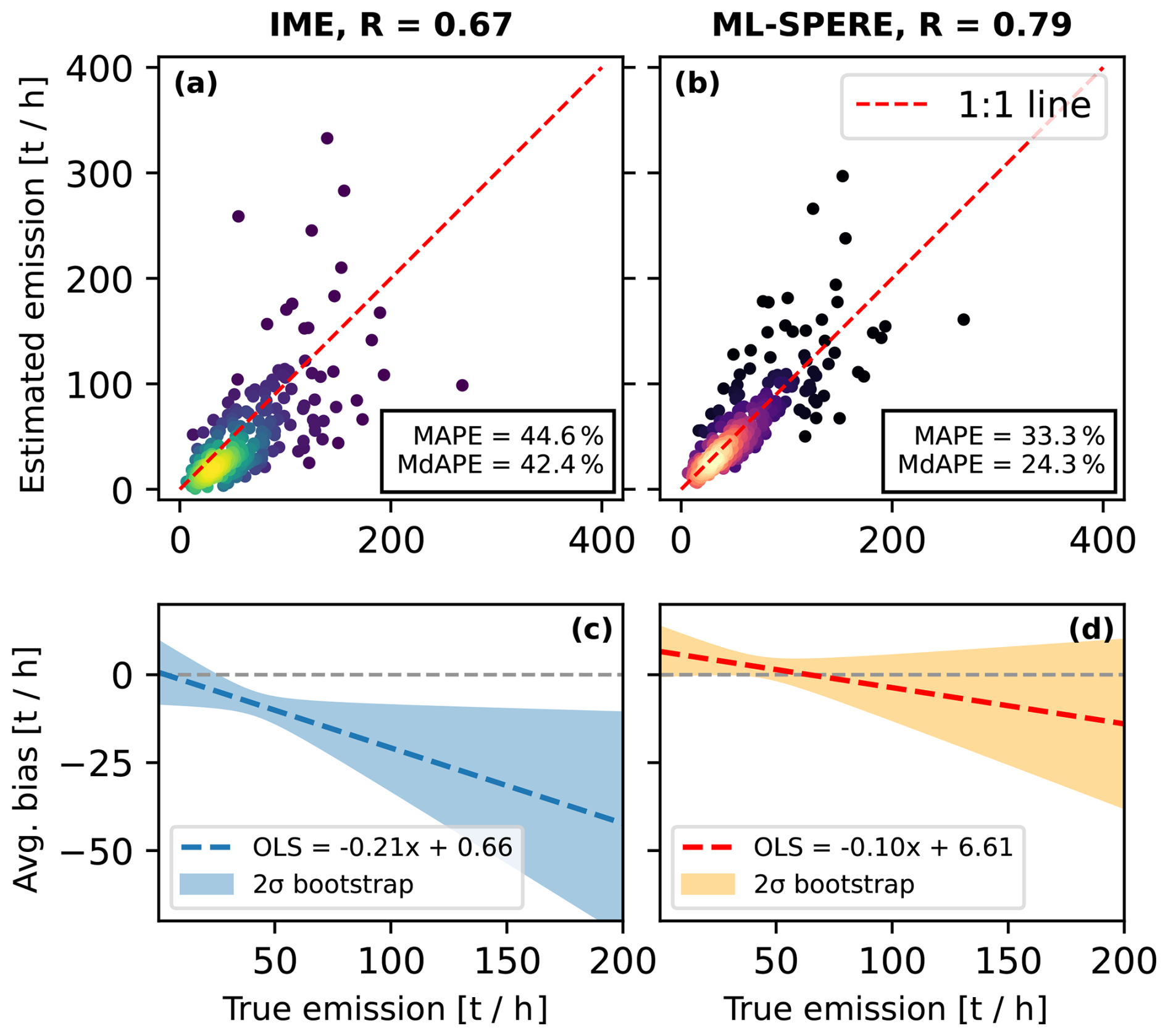
Figure A4 Estimated emission rates for simulated HYSPLIT plumes via (a) the IME method and (b) ML-SPERE as a function of true plume emission rates, filtered to only include scenes from the test set where the emission source location is contained within the estimated plume mask. The colormaps represent the relative density of the visualised data. We visualise bootstrapped ordinary least squares (OLS) regression lines for emission rate estimates from both the IME method (in c) and ML-SPERE (in d). The 1:1 line is subtracted in (c) and (d) to show average bias.

We investigate this directly by visualizing the partial gradient of the ML-SPERE emission rate estimate with respect to the pixels in the methane channel of the input image, as shown in Fig. A5. The gradients in Fig. A5b indicate that increasing methane concentrations immediately upwind of the source pixel decreases the emission-rate estimate, whereas increasing concentrations at the source pixel or in pixels immediately downwind increases the estimate. This behavior follows directly from mass-balance considerations and shows that ML-SPERE has learned to use methane enhancement gradients aligned with the wind vector to generate emission-rate predictions. Information in the plume tail is less influential, as reflected by the weaker gradients in that region in Fig. A5b.

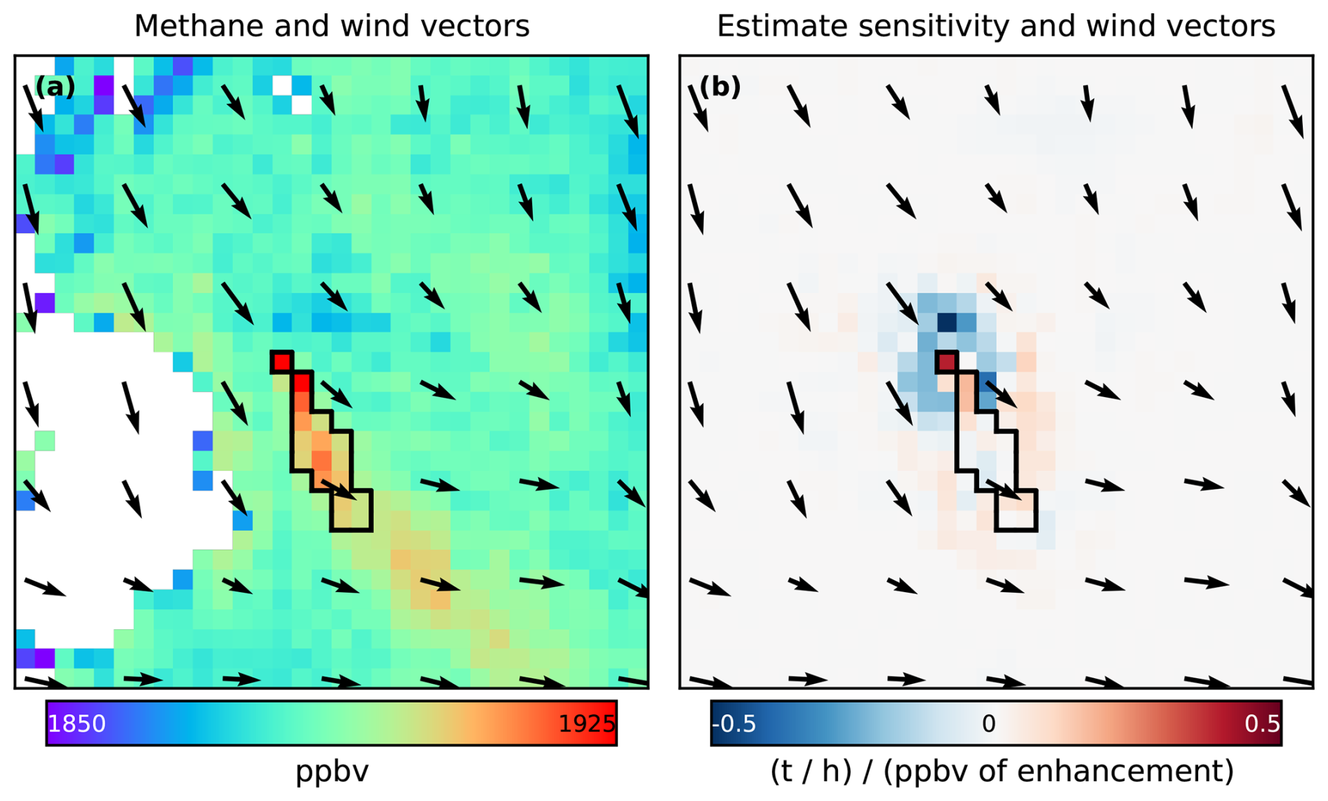
Figure A5 A methane scene from the test set (a) and the corresponding gradients between the emission rate estimated by ML-SPERE and the pixels in the methane channel (b). Gradients are strongest around the head of the plume.

A4 ML-SPERE and IME uncertainty estimates

The probability integral transform (PIT), originally formalized by David and Johnson (1948), provides an estimate of posterior calibration by recording, for a set of samples, the percentile ranks of the true values within their respective predicted posterior distributions. In the context of this work, we can construct PIT histograms for both ML-SPERE and the IME method by evaluating the cumulative distribution function of each emission rate posterior distribution (e.g. for each plume in the simulated test set) at the corresponding true value. An example for a single plume's posterior emission rate estimate is shown in Fig. A6a. For a well-calibrated model, these percentiles should be uniformly distributed when taken for a large sample of plumes.

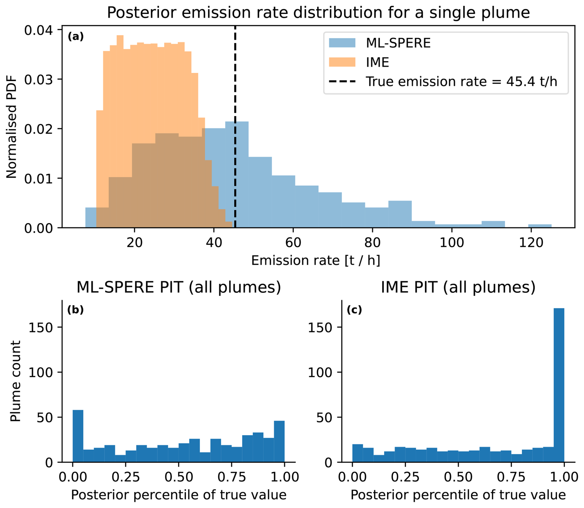
Figure A6 (a) Examples of estimated posterior emission rate distributions for a single scene via both ML-SPERE and the IME method. The true emission rate for this plume (45.4 t h⁻¹) lies at a posterior percentile of 0.57 for ML-SPERE, and 1 for the IME method. Calculating and binning such values for both methods and all plumes in the synthetic test set generates (b) the PIT for ML-SPERE and (c) the PIT for the IME method.

The PIT histograms for ML-SPERE (Fig. A6b) and the IME method (Fig. A6c) reveal differing calibration characteristics between the two methods. For ML-SPERE, the distribution exhibits the largest values in the outermost bins. This indicates a tendency to generate narrow uncertainty bands that do not always capture the true emission rate of the plume, though as discussed in Sect. 3.1 and shown in Fig. A6, the uncertainty ranges on ML-SPERE estimates capture true emission rates more often than those of the IME method. In contrast, the IME method exhibits a pronounced spike at the upper bound (100th percentile), alongside an otherwise roughly uniform distribution. This accumulation at the upper tail indicates a systematic tendency to underestimate emission rates, such that true emission rates frequently exceed the upper bound of the estimated uncertainty range. Together, these results suggest that while both methods underestimate uncertainty, ML-SPERE provides better-calibrated and less biased posterior estimates than the IME approach.

The synthetic test set plumes were simulated using HYSPLIT with ERA5 wind data while ML-SPERE was trained using plumes simulated with WRF-Chem and NCEP wind data. Similarly, the IME effective wind speed calibration shown in Eq. (2) and given in Schuit et al. (2023a) was estimated using a synthetic plume set also simulated by WRF-Chem using NCEP wind data. The results shown in Fig. A6 therefore suggest that ML-SPERE (and the methods used for estimating uncertainties outlined in Sect. 2.4) extrapolates better across different simulated plume datasets than the IME method implemented here does.

A5 K-fold cross validation analysis

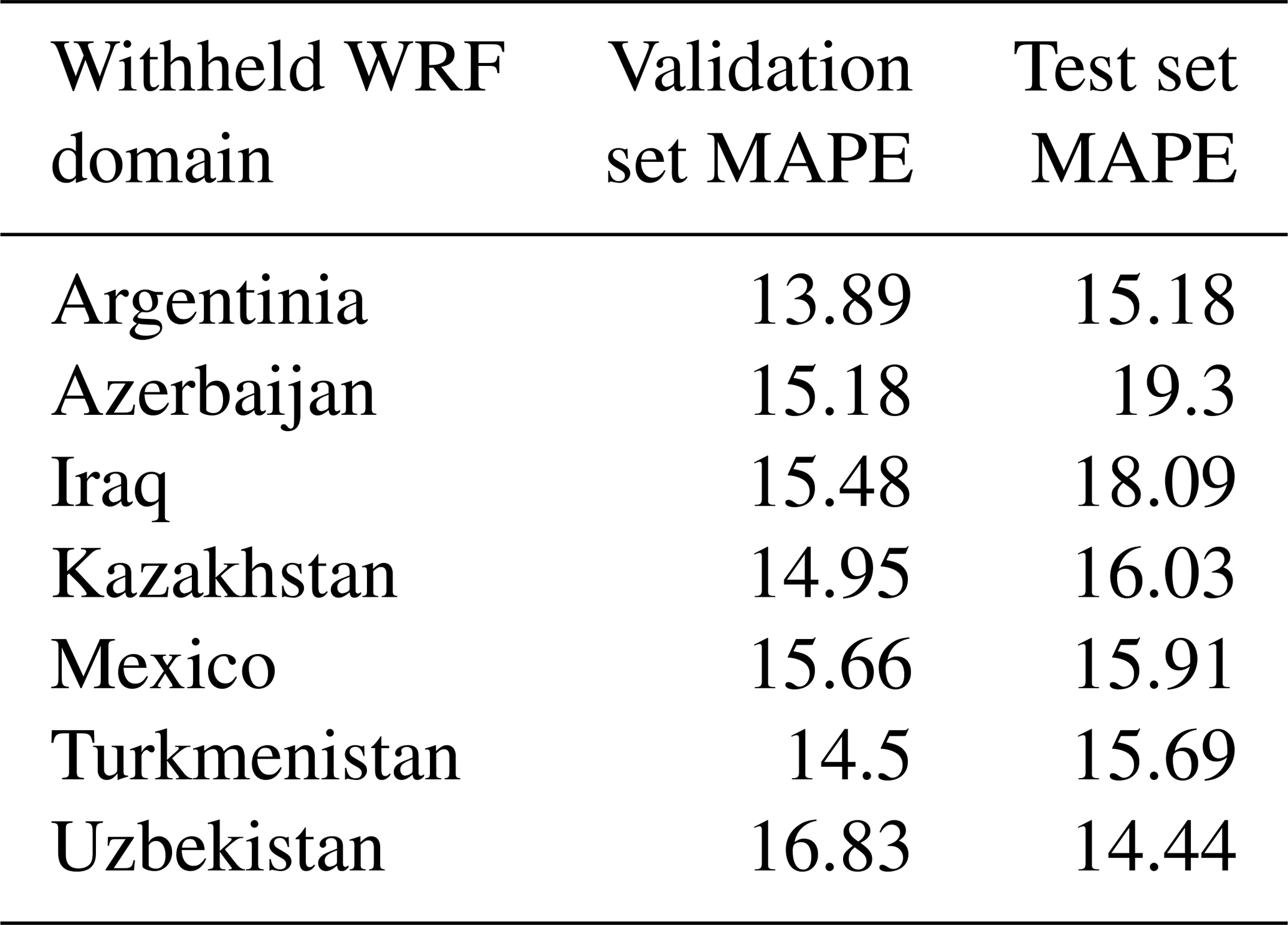
To assess model generalization prior to training ML-SPERE on the full training and validation dataset, we conducted a K-fold cross-validation across the seven used WRF-Chem domains shown in Fig. A1. In each fold, the model was re-trained while withholding plumes from one WRF-Chem domain as a cross-validation test set, with the remaining plumes partitioned into training and validation subsets. The results of this K-fold analysis are presented in Fig. A7 and Table A2. Model fitting converges to comparable performance levels across folds. For all domains except Uzbekistan, the withheld test set performance is slightly lower than validation set performance. This outcome is expected, as the test sets are constructed to be independent from the training and validation data along the relevant dimension of variability, which in this case is the geographic location of plumes.

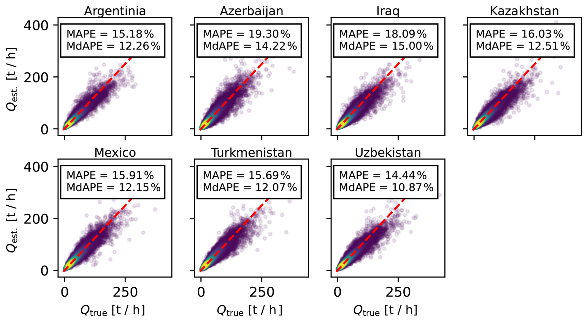
Figure A7 Visualizations of ML-SPERE estimated emission rates Q_est. vs. true emission rates Q_true for each of the K-fold test sets. Values for MAPE and MdAPE are shown in each panel, and the red dashed lines show the 1:1 line. The colormaps represent the relative density of the visualised data.

Table A2 Test and validation set performance for each of the K-fold datasets created before final model fitting.

A6 Examining changes in ML-SPERE performance when estimating emission rates for HYSPLIT plumes vs. WRF-Chem plumes

We produced three synthetic plume sets for a cluster of four coal mines in Kazakhstan for the year 2022, temporally sampled with daily output at the TROPOMI overpass hour and spatially resampled to the TROPOMI pixel footprints of the corresponding TROPOMI orbit. In the first set, plumes were simulated with WRF-Chem using NCEP meteorology for boundary conditions, which corresponds to the settings used to create the training and validation set plumes used to train ML-SPERE. In the second plume set, plumes were simulated with WRF-Chem using ERA5 meteorology for boundary conditions. In the third plume set, plumes were simulated with HYSPLIT using ERA5 meteorology for particle transport, which mimics the global set of plumes used as a test set for ML-SPERE in Sect. 3.1. Across all three datasets, plumes were sampled at identical times, resampled to identical TROPOMI pixel orbit geometries, and use identical TROPOMI background data to produce a realistic scene.

Figure A8 shows ML-SPERE estimates against true emission rates for each of these plume sets. ML-SPERE estimates for the plume sets simulated with WRF-Chem exhibit values of MAPE and MdAPE similar to those seen in the K-fold cross validation analysis of Sect. A5 (which did not include methane backgrounds or missing data), but the plume set simulated with HYSPLIT exhibits higher values of MAPE and MdAPE that are similar to the results of Sect. 3.1. A visual inspection of these plume sets shows that the two plume sets simulated with WRF-Chem look very similar, despite using different meteorological datasets as boundary conditions, while the plumes from the HYSPLIT set can at times exhibit different morphologies, sometimes appearing more diffuse than the WRF-Chem plumes. This suggests that the difference in performance that ML-SPERE shows between the K-fold cross validation analysis and the test set results in Sect. 3.1 is driven by morphological differences between plumes simulated by WRF-Chem and HYSPLIT, and is not due to the change in meteorological data between the training data and the test data or the greater geographic range of plumes simulated in the test set. WRF-Chem and HYSPLIT can simulate plumes that are different from each other for a variety of reasons. WRF-Chem can only simulate “point sources” at a resolution equivalent to the native grid of the simulation, whereas HYSPLIT simulates particle emission at an actual point. Furthermore, WRF-Chem uses meteorology as boundary conditions for a spatial domain, whereas HYSPLIT uses meteorology to directly transport particles throughout a spatial domain and can be sensitive to diffusion parameterizations.

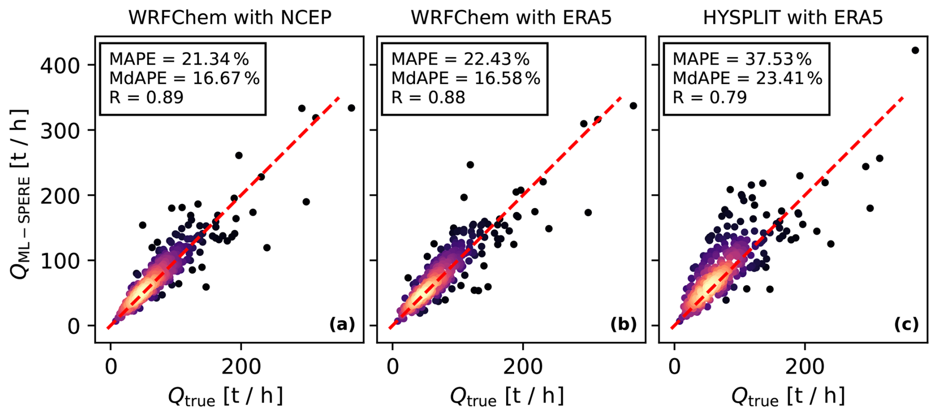
Figure A8 ML-SPERE emission rate estimates (Q_ML-SPERE) as a function of true plume emission rates (Q_true) for three plume sets simulated for coal mines in Kazakhstan. Subpanel titles indicate the chemical transport code (either WRF-Chem or HYSPLIT) and the wind data (either NCEP or ERA5) used to simulate the plumes. ML-SPERE performance on plume sets simulated with WRF-Chem (panels a and b) is comparable to that of the validation plume set, whereas performance on the HYSPLIT plume set (panel c) is modestly degraded. This demonstrates that reduced test set performance arises primarily from differences in the transport models used to generate the plumes of the training and test sets, and not the global extrapolation. The colormaps represent the relative density of the visualised data.

A7 ML-SPERE estimates for Karaturun East 2023 blowout

In Table A3, we present the ML-SPERE emission rate estimates corresponding to the data from Fig. 5. The table also reports the estimated contributions to the total uncertainty from plume masking, background removal, wind field error, and model error.

Table A3 ML-SPERE emission estimate metrics by date for the Karaturun East 2023 blowout in Kazakhstan. Q refers to the posterior distribution of estimated emission rates obtained from the procedure described in Sect. 2.4. Q_median is the median of the posterior distribution of estimated emission rates. Q_σ is the standard deviation of the posterior distribution of estimated emission rates. Q₁₆ and Q₈₄ are the 16th and 84th percentiles of the posterior distribution of estimated emission rates, respectively. Wind, masking, background, and model error are all estimated as described in Sect. 2.4 (i.e. they do not sum to Q_σ). All table values are [t h⁻¹].

A8 Geographic trends in ML-SPERE and IME estimate residuals for the 2021 TROPOMI methane detection plume set

In Fig. A9, we show mean standardised logratios between ML-SPERE and IME estimates for the plumes catalogued in Schuit et al. (2023b) on a 15° global grid. This allows us to examine the ratios of estimates obtained via ML-SPERE and the IME method in terms of standard deviations away from the mean ratio of the two methods across the entire dataset, and determine if there are any significant regional trends in the differences between estimates obtained via the two methods (defined as being either greater than 0.5 standard deviations or less than −0.5 standard deviations of the dataset-wide mean standardised logratio). The figure shows that statistically significant regional differences between ML-SPERE and IME emission-rate estimates occur primarily in northern Russia and southeastern Australia (where ML-SPERE estimates are systematically higher) and in the Congo region (where ML-SPERE estimates are systematically lower). For all these regions, we have a small sample size of plumes to examine.

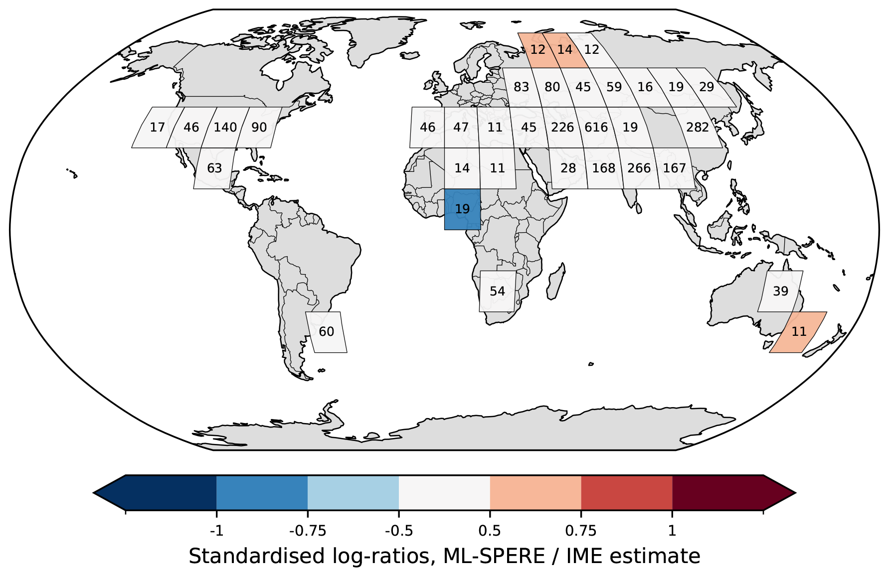
Figure A9 Global standardised logratios between emission rate estimates from ML-SPERE and the IME method for the plume set of Schuit et al. (2023b), expressed as mean per grid cell. Number of plumes are plotted in each grid cell.

A8.1 ML-SPERE estimates for plumes in northern Russia

We find that ML-SPERE estimates for detected plumes in northern Russia are on average higher than those from the IME method, with mean standardised logratios 0.5–0.75 standard deviations above the dataset-wide mean. Although the true emission rates for these plumes are unknown, the average IME estimate for plumes in this region are 34 t h⁻¹. Figure 3d shows that ML-SPERE may overestimate emissions for plumes with true emission rates below 50 t h⁻¹ due to regression dilution, if no human oversight is used to limit the application of ML-SPERE to plumes that are well-observed and have complete spatial information around the plume head.

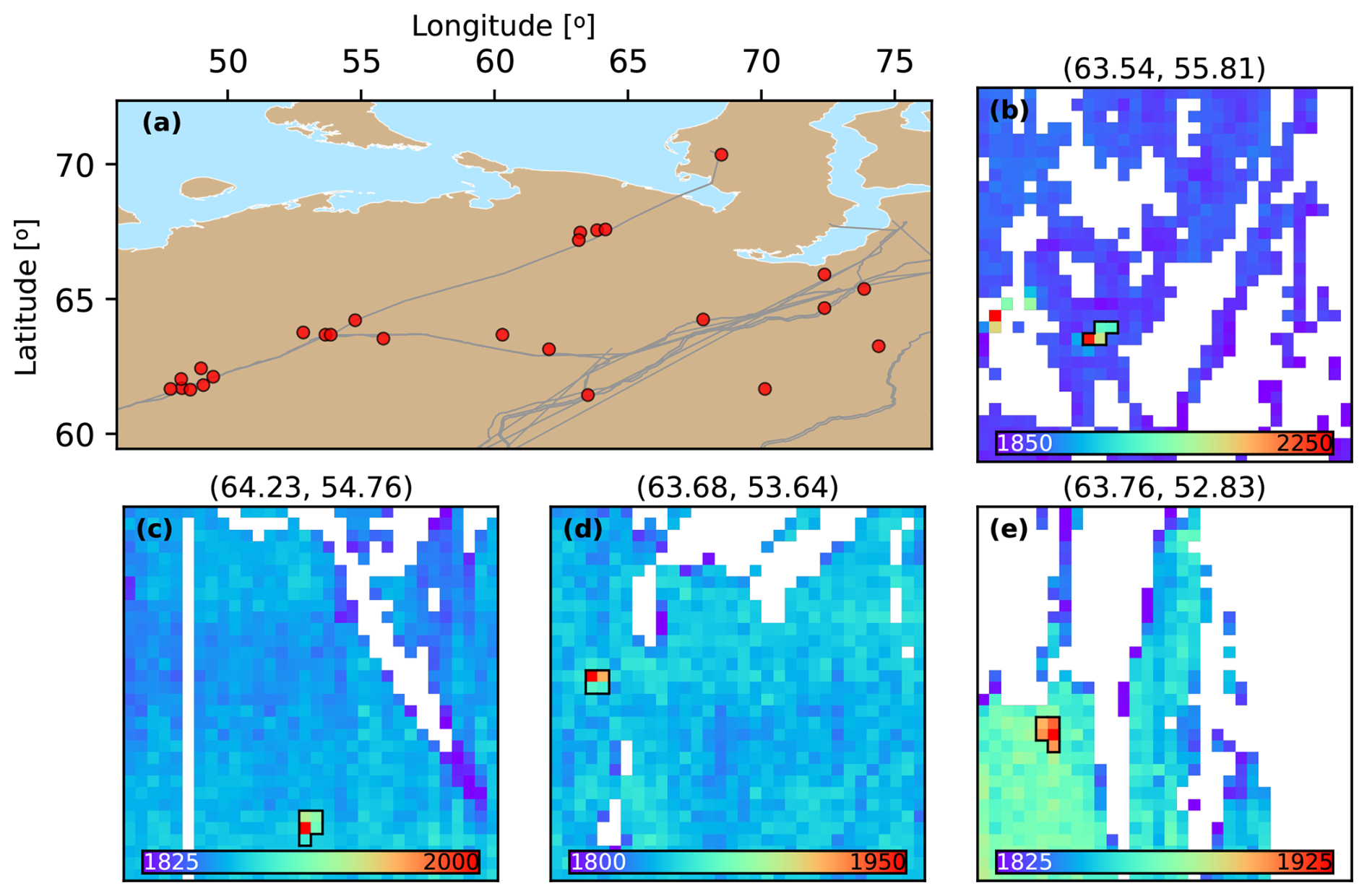
Figure A10 (a) Locations for the plumes in northern Russia for which ML-SPERE estimates exhibit the largest log-ratios when compared to the IME method, shown in red dots. Pipelines from the Global Energy Monitor are shown with grey lines. Examples of methane observations are shown in panels (b–e), and colorbar values show methane concentrations in ppbv. Latitude-longitude coordinates of the most upwind pixel within the plume masks are shown in the titles of panels (b–e).

Mapping the locations of these plumes shows that they coincide with known natural gas pipeline infrastructure. Visual inspection shows that these scenes contain extremely compact, blob-like methane enhancements with very high concentrations (Fig. A10). Such features are characteristic of transient emissions (e.g. blowdowns at block valves) rather than the steady-state plumes on which ML-SPERE was trained. As shown in Sects. 3.1 and A3, ML-SPERE relies heavily on methane enhancement gradients aligned with local wind vectors to infer emission rates. It is therefore plausible that ML-SPERE may overestimate emission rates for short-duration, highly concentrated emissions where mass-balance structure differs from that of steady-state plumes.

As discussed in Sect. 3.1, human oversight is essential when applying ML-SPERE (though this holds for all methods and not only for ML-based methods). Transient, non steady-state emissions may not be well estimated by either ML-SPERE or the IME method, and total plume mass may be more relevant. Finally, although ML-SPERE yields higher estimates than the IME method in these cases, the true emission rates are still unknown, and we cannot say with certainty that ML-SPERE estimates for these specific plumes were less accurate than IME estimates.

A8.2 ML-SPERE estimates in the Congo basin

As shown in Fig. A9, ML-SPERE estimates for plumes in the Congo Basin are on average lower than the corresponding IME estimates. Visual inspection of these scenes reveals very large plumes that are frequently spatially disrupted by cloud cover or by gaps in TROPOMI retrievals over water. As discussed in Sects. 3.1 and A3, ML-SPERE performs best when the region surrounding the plume head or emission source is well observed, and analyst judgment may be required when these conditions are not met. The Congo Basin plumes are also on average approximately 50 % larger than those in the training dataset, potentially reflecting more spatially diffusive emitters than those represented in the simulations. Consequently, ML-SPERE may be less well suited for application to these scenes, though it is important to recognize that the IME method was not designed to be applied to area-source emissions. Both methods may struggle to characterize emissions in this region.

A8.3 ML-SPERE estimates in Australia

For the 11 plumes in the grid cell in southwestern Australia in Fig. A9, ML-SPERE estimates are on average higher than IME estimates. Inspection of these plumes show that they have low wind speeds below 2 m s⁻¹ and average emission rates estimated via the IME method at 14 t h⁻¹. This suggests that although this may be an emission rate regime where ML-SPERE may overestimate emissions due to regression dilution, it is also possible that the IME method is underestimating emissions due to the low wind speed bias outlined in Sect. 3.1. This bias is hinted at operationally for the entire 2021 plume dataset in Fig. 6b.